reynolds number effects on leading edge vortices
TRANSCRIPT

Page 1
When Are Reynolds No. Effects Important ?
Reynolds Number Effects on Leading Edge Vortices
Taken From AIAA-2002-2839 Paper“Reynolds Numbers Considerations for Supersonic Flight”
Brenda M. Kulfan32nd AIAA Fluid Dynamics Conference and Exhibit
St. Louis, Missouri 24 - 26 June 2002
The viability of a high-speed civil transport,HSCT, is very dependent on its cruise aerodynamic performance. The nature of the flow over a supersonic configuration changes through out its operating flight regime from low speed take off and landing condition, through subsonic cruise, transonic acceleration to supersonic cruise. Reynolds number and Mach number are the most familiar flow similarity parameter for aircraft applications. Two different scale models possess geometric similarity if the corresponding geometric dimensions of each model are all related by a single length scale factor. Matching the Reynolds number and the Mach number over two geometrically similar models will insure that the flows over each model will be dynamically similar in that the streamline patterns are geometrically similar, the general nature of the flows ( e.g. turbulent or laminar, attached or separated) will be identical and the dimensionless force coefficients are also the same. The performance characteristics of an HSCT, as well as the effectiveness of the control surfaces may be very dependent on Reynolds Number as well as the flight Mach number. The Reynolds number consequently is the primary aerodynamic scaling parameter used to relate sub-scale wind tunnel model experiments to full scale airplanes in flight.A number of recent investigations have focused on the effects of Reynolds number on HSCT type configurations in the subsonic high lift conditions 1, transonic cruise / climb conditions 2 as well as on the stability and control characteristics 3 over the same flight regimes. Similar investigations have been made for fighter type configurations 4, 5.

Page 2
• Wind Tunnel Test Limitations Reynolds Number Questions and ConcernsRelative to the Design, Performance and Viability of an HSCT.
• Discuss Fundamental Nature of Flow Over HSCT Type Configuration At Design and Off Design Conditions
• Use Simple Flow Analogies and Aerodynamic “Tools” to Examine Leading Edge Vortex Flow
• Attempt to Identify Reynolds Numbers Effects On:– Leading Edge Vortex Development– Leading Edge Vortex Bursting
• Evaluate CFD Predictions of the Flow Features, Forces,Moments and Pressures.
Topics
This paper will focus on the effects of Reynolds number on HSCT type configurations over the supersonic climb / cruise portions of the flight envelop. Many of the discussions and conclusions will apply equally to military type aircraft operation in a similar flight regime having similar geometric features. Specific design features and aerodynamic characteristics, which may be significantly influenced by Reynolds number, will be discussed. Current wind tunnels Reynolds number testing capabilities will be reviewed. It will be shown that the existing testing limitations lead to a number of fundamental questions and concerns relative to the design, performance and viability of a High Speed Civil Transport,HSCT, configuration.The general nature of possible types of surface flow, that a supersonic aircraft may encounter within its flight regime, will be summarized. Simplified flow analogies along with wind tunnel data and CFD computational results will be used to explore the dependency of the flow characteristics on specific geometric design features of an aircraft as well as upon Reynolds number. Specific Reynolds number effects will be explored in three general areas:
• Attached flow conditions typically associated with the cruise conditions• Shock / boundary layer interactions at near cruise conditions• Leading edge vortex flow at off design conditions
In the process, assessments will be made of the ability of the inviscid and Navier Stokes CFD methods to predict flow features, forces, moments and pressures at both wind tunnel and flight conditions.We will also attempt to answer the intriguing questions:
• Will the difference between a low Reynolds number viscous CFD calculation and a corresponding inviscid CFD calculation always “Bracket” the flow characteristics at full scale conditions?
• Is shock induced boundary layer separation strongly influenced by Reynolds number?• Does Reynolds affect the movement of the origin of a leading edge vortex on a swept wing with a round
leading edge?It will be shown that coordinated wind tunnel test programs and extensive code validation studies will be necessary to properly predict and understand full scale conditions.
Page 3
NTF (-250oF), 2.20%q = 2700 psf
ETW (-250oF), 1.94%
ARC 12 ft, 2.81%
LaRC 16 ft, 3.81%
ARC 11 ft, 2.96%
BTSWT 4 ft, 1.70%
Rey
nold
s N
umbe
r, M
illion
s400
80
100
200
60
40
20
108
6
4
20 0.2 0.4 0.6 0.8 1.0 1.2 1.4 1.6 1.8 2.0 2.2 2.4 2.6
Mach Number
Supersonic ClimbAnd
Supersonic Cruise
High LiftOperation
Subsonic Cruiseand
Transonic Climb
HSCT Wind Tunnel Testing Dilemma
NTF (-250oF), 2.20%q ,max
Oh My !
HSCT Flight EnvelopeFull Scale
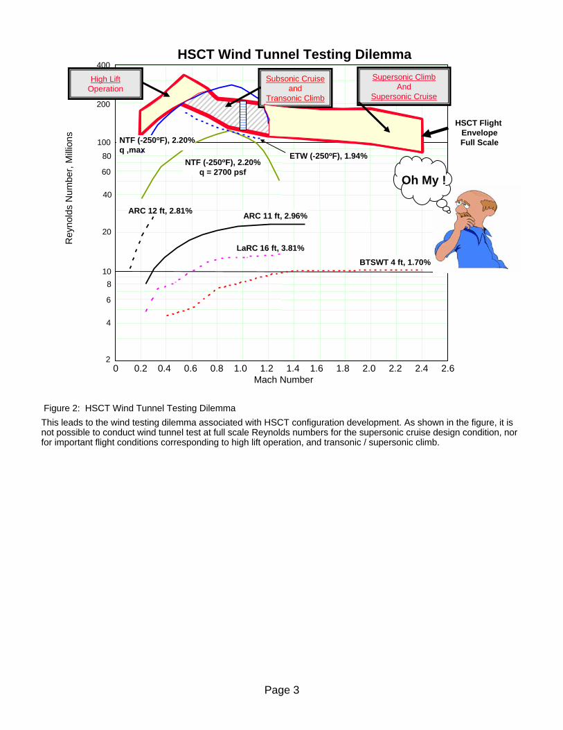
Figure 2: HSCT Wind Tunnel Testing DilemmaThis leads to the wind testing dilemma associated with HSCT configuration development. As shown in the figure, it is not possible to conduct wind tunnel test at full scale Reynolds numbers for the supersonic cruise design condition, nor for important flight conditions corresponding to high lift operation, and transonic / supersonic climb.

Page 4
Rey
nold
s N
umbe
r, M
illio
ns
400
80
100
200
60
40
20
108
6
4
20 0.2 0.4 0.6 0.8 1.0 1.2 1.4 1.6 1.8 2.0 2.2 2.4 2.6
Mach Number
Wind tunnel to Flight Scaling Strategies
Supersonic WT Experiments and CFD Validation
1. Skin Friction Drag Corrections 2. CFD Prediction Increments +
Viscous Drag Extrapolation
Transonic WT Experiments and CFD Validation
NTF WT Experiments and
CFD Validation
Validate Skin Friction Predictions
3. CFD Predictions ofForces and Moments
1. Skin Friction Drag Corrections 2. CFD Prediction Increments +
Viscous Drag Extrapolation
Three options are generally available to generate aerodynamic data at the flight Reynolds numbers:1. Simple flat plate skin friction theory is used to extrapolate the wind tunnel data to full scale conditions. This is
typically the approach used to generate the extensive performance database required for the development of a commercial aircraft configuration.
2. Calibrated CFD methods are used to calculate the aerodynamic data for both the wind tunnel model and the full scale airplane. The theoretical increments between the two sets of data are applied to the wind tunnel database to obtain either the full scale performance, or to obtain an adjusted database which is then extrapolated to full scale conditions using the flat plate skin friction theory.
3. Use the wind tunnel to evaluate and calibrate the CFD methods. The CFD methods are then used to predict the performance and flow characteristics at full scale conditions. This is the typical approach used for aerodynamic evaluations during the design development process.
There are a number of assumptions inherent in each of these options. The key assumption of the first option is that the fundamental flow physics on the wind tunnel model are unaffected by the Reynolds number differences between the model at test conditions and the airplane at flight conditions. It is therefore also assumed that the pressure related forces and moments are essentially the same on the model and the airplane. Therefore the only difference in aerodynamic forces between the airplane and the wind tunnel model is in the viscous drag force. The final assumption is that the viscous drag difference can be determined as the increment between simple flat plate theory skin friction predictions on the airplane and on the wind tunnel model at the corresponding Mach numbers.The fundamental assumption of the second option is that CFD methods can capture correctly the differences in nature of flow physics on the airplane and on the wind tunnel model and therefore and can also adequately predict the associated changes in the viscous and pressure forces and moments.The adjusted wind tunnel data is then extended to full scale conditions either as in option 1 or by CFD calculations on the airplane at the flight conditions. The third options precludes the use of wind tunnel data and assumes that the CFD predictions can adequately predict the flow physics and associated forces and moments on the airplane at flight conditions. This is often used to check the aerodynamic performance of the airplane at a limited number of flight conditions during the aerodynamic design process.With any of these options adjustments must be made to account for differences between the wind tunnel model geometry and the airplane, and to include additional drag adjustments to account for excrescence drag, power effect related drag items and other miscellaneous drag items.Coordinated CFD and wind tunnel validation studies are very necessary to establish the validity and the consistency of the CFD predictions.

Page 5
The inability to test at full scale conditions plus the uncertainties in the adequacy of CFD predictions, result in a number of fundamental Reynolds Number questions related to the design and aerodynamic assessment of a HSCT:Can we predict the flight performance, stability levels and control effectiveness? Can we make correct configuration design decisions?Are the right high lift systems and control surfaces being developed?When is testing at low Reynolds adequate?When is testing at high Reynolds number required?Can CFD codes, validated with low Reynolds number data, adequately predict forces, moments and flow characteristics at full-scale conditions?Will the final design meet the design criteria and performance guarantees?
Reynolds Number Concerns
• CAN WE PREDICT FLIGHT PERFORMANCE, STABILITY LEVELS AND CONTROLEFFECTVENESS?
• CAN WE MAKE CORRECT CONFIGURATION DECISIONS ?
• WHEN IS TESTING AT LOW REYNOLDS NO. ADEQUATE?
• WHEN IS TESTING AT HIGH REYNOLDS NUMBER REQUIRED?
• CAN CFD CODES VALIDATED WITH LOW REYNOLDS NUMBER TEST DATA, ADEQUATELY PREDICT FORCES, MOMENTS AND FLOW CHARACTERISTICS AT FULL SCALE CONDITIONS ?
• CAN WE VALIDATE DESIGNS OPTIMIZED FOR FULL SCALE REYNOLDS BY LOW REYNOLDS NUMBER WIND TUNNEL TESTS
• ARE WE DEVELOPING THE RIGHT HIGH-LIFT SYSTEMS AND CONTROL CONCEPTS?
• CAN WE MEET DESIGN CRITERIA AND PERFORMANCE GUARANTEES?
Page 6
Aerodynamic Investigative Tools Searching for the Clues
EXPERIMENTALFLUID DYNAMICS
(WIND TUNNEL)“EFD”
“UFD” UNDERSTAND FLUID DYNAMICS (WISDOM)
• Nature of the Flow On Supersonic Configurations– Attached Flow– Separated Flow– Shocks– Vortex Flow– Vortex Bursting
• Simple Flow Analogy Studies
• Wind Tunnel Experimental Results– Forces and Moments– Flow Visualization– Pressure Measurements
• CFD Studies and Predictions
• CFD Viscous versus Inviscid Predictions
• Wind Tunnel and Flight Test Correlations
• Explore Fundamental Controlling Effects– Geometry ( Planform, Leading edge shape, etc)– Mach Number– Reynolds Number– Angle of Attack– Surface Deflections
“CFD”COMPUTATIONALFLUID DYNAMICS
(NUMERICAL)
“VFD”VISUAL
FLUID DYNAMICS(CFD & EFD)
“RFD”REAL
FLUID DYNAMICS(FLIGHT TEST)
“SFD”SIMPLIFIED
FLUID DYNAMICS(ANALOGIES)
“AFD”APPROXIMATE
FLUID DYNAMICS(EMPIRICAL)
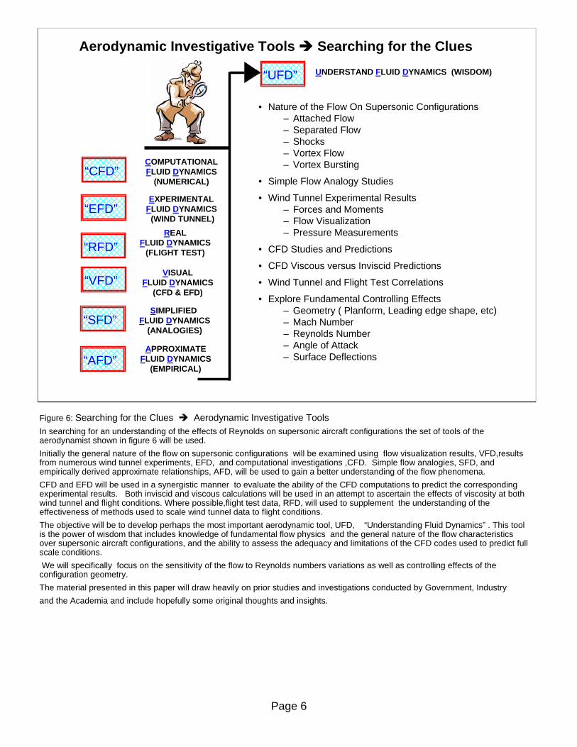
Figure 6: Searching for the Clues Aerodynamic Investigative ToolsIn searching for an understanding of the effects of Reynolds on supersonic aircraft configurations the set of tools of the aerodynamist shown in figure 6 will be used.Initially the general nature of the flow on supersonic configurations will be examined using flow visualization results, VFD,results from numerous wind tunnel experiments, EFD, and computational investigations ,CFD. Simple flow analogies, SFD, and empirically derived approximate relationships, AFD, will be used to gain a better understanding of the flow phenomena. CFD and EFD will be used in a synergistic manner to evaluate the ability of the CFD computations to predict the corresponding experimental results. Both inviscid and viscous calculations will be used in an attempt to ascertain the effects of viscosity at both wind tunnel and flight conditions. Where possible,flight test data, RFD, will used to supplement the understanding of the effectiveness of methods used to scale wind tunnel data to flight conditions.The objective will be to develop perhaps the most important aerodynamic tool, UFD, “Understanding Fluid Dynamics” . This tool is the power of wisdom that includes knowledge of fundamental flow physics and the general nature of the flow characteristics over supersonic aircraft configurations, and the ability to assess the adequacy and limitations of the CFD codes used to predict full scale conditions.We will specifically focus on the sensitivity of the flow to Reynolds numbers variations as well as controlling effects of the
configuration geometry.The material presented in this paper will draw heavily on prior studies and investigations conducted by Government, Industry and the Academia and include hopefully some original thoughts and insights.

Page 7
Various Types of Flow on Highly Swept Wings at Supersonic Speeds
SupersonicSlightly Off Design
Possible ConditionsWithin Flight Envelope
SupersonicDesign Condition
Figure 7: Various Types of Flow on Highly Swept Wings at Supersonic Speeds
Figure 7 shows the types of flows that have been observed over a class of supersonic wing planforms having highly swept subsonic leading edges and supersonic trailing edges8,9. Many of these flow features have also been observed on hybrid planforms having a combination of subsonic and supersonic leading edges.At the primary supersonic cruise condition, an aerodynamically efficient wing is designed to have attached flow over the entire wing surface. With a supersonic trailing edge, the flow over the upper surface will encounter a trailing edge shock as it readjusts to the local free stream conditions.The trailing edge shock will not be initially sufficiently strong to separate the flow over the wing.At slightly off design conditions, weak oblique shocks may develop on the upper surface. Depending on the sweep of the trailing edge, strong span wise flow may develop in the region of the trailing edge. At off design conditions the wing may encounter a combination of separated flow behind shocks that originate near the leading edge as well as flow separation due to the increased strength of the trailing edge shock. Because of the thin highly swept leading edges, the flow may separate as it flows from the lower surface attachment line around the leading edge to the upper surface forming coiled up leading edge vortices.
Page 8
Typical Characteristic Flow Over Thin Slender Wings
Attached Flow Leading-EdgeVortex Flow
PartialLeading-EdgeVortex Flow
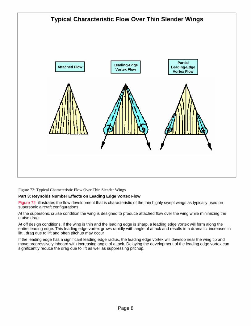
Figure 72: Typical Characteristic Flow Over Thin Slender WingsPart 3: Reynolds Number Effects on Leading Edge Vortex FlowFigure 72 illustrates the flow development that is characteristic of the thin highly swept wings as typically used on supersonic aircraft configurations.At the supersonic cruise condition the wing is designed to produce attached flow over the wing while minimizing the cruise drag. At off design conditions, if the wing is thin and the leading edge is sharp, a leading edge vortex will form along the entire leading edge. This leading edge vortex grows rapidly with angle of attack and results in a dramatic increases in lift , drag due to lift and often pitchup may occurIf the leading edge has a significant leading edge radius, the leading edge vortex will develop near the wing tip and move progressively inboard with increasing angle of attack. Delaying the development of the leading edge vortex can significantly reduce the drag due to lift as well as suppressing pitchup.

Page 9
ΛLE = 50O ΛLE = 60O
ΛLE = 70O
ΛLE = 75O
0.5 1.0 1.5 2.0 2.5 3.0 3.5Mach Number
20
15
10
5
0
α deg
Attached Flow
LE VortexFlow
Leading Edge Vortex Formation Boundaries for Flat Sharp Swept Wings
Figure 10: Leading Edge Vortex Formation Boundaries for Flat Sharp Swept Wings
Another flow feature common to highly swept thin wing planforms, is the appearance of leading edge vortices as the angle of attack is increased. By virtue of extensive experimental and semi-empirical investigations 10 to 16, the formation of the leading edge separation vortex is well understood. On a supersonic wing, the leading edge vortex can develop providing that the component of Mach number normal to the leading is subsonic. Experimental investigations have established the boundary shown figure 10 that divides the regions for attached flow and for leading edge separated flow for flat wings with thin sharp leading edges.The separation boundary is defined in terms of the Mach number normal to the leading edge, MN, and the angle of attack normal to the leading edge αN, by the expression:MN = 0.6 + 0.013 αNMN and αN are defined in terms of the free stream Mach number, angle of attack and leading edge sweep in the figure.The separation boundary layer equation has been used to construct the chart in the lower right side of figure 10 that shows the variation of the separation boundary layer with leading edge sweep for a wing with a straight leading edge.

Page 10
Attached Flow
Upper Surface Flow Characteristics Over Delta wings at Supersonic Speeds
Figure 11: Upper Surface Flow Characteristics Over Delta wings at Supersonic Speeds
The results of extensive wind tunnel investigations of the nature of the flow over flat swept wings with thin sharp leading edge expanded the identification of boundaries between the various classes of flows17 as shown in Figure 11.
For wing planforms in which the leading edge is swept behind the free stream Mach line, the use of wing camber along with round leading edge airfoils can result in a region of attached flow at low angles of attack , and to shift the other boundaries to higher angles of attack. However, similar classes of flows such as shown in figure 11 may ultimately be expected to form on even these wing designs.

Page 11
LEX
Chines
Notched Trailing Edge
Arrow Wing
Geometry Variations Affecting Supersonic Flow Characteristics
Figure 12: Geometry Variations Affecting Supersonic Flow CharacteristicsAs shown in figure 12, supersonic aircraft configurations may encompass a wide variety design features. The features of each design will ultimately determine the unique nature of the flow characteristics over its operating envelop. However, for each configuration, the three classes of flows may be expected to ultimately develop somewhere within its flight envelop. These include conditions that are primarily dominated by:
1. attached flow2. shock / boundary layer induced separations 3. leading edge vortex flows
The paper will focus on identifying the effects of Reynolds number differences between typical wind tunnel test conditions and full scale conditions on these three general classes of flows in the above order. The format of the paper will therefore, be composed of three major sections corresponding to the three general classes of flows.
Engine Integration

Page 12
Reynolds Number Effects on Leading Edge Vortex Development and Effects~ Changes Between Wind Tunnel and Flight ~
• Simple Flow Analogies (SFD), to Explore:– Fundamental Nature of Leading Edge Vortices– Effect Of Wing Geometry On Leading Edge Vortex Development– Leading Edge Vortex Development at Supersonic Speeds
• Wind Tunnel Experimental Investigations (EFD), of Reynolds Number Effects on Leading Edge Vortex Development
• Euler and Navier Stokes Predictions (CFD), of Leading Edge Vortex on Pressures, Forces and Moments
• Flow Visualization Results From EFD and CFD Studies for Insight into Details of Leading Edge Vortex Flow
• Develop an Understanding (UFD) of Reynolds Number and Mach number Effects on Leading Edge Vortices.
In this section, simple flow analogies (SFD) will be used to explore the fundamental nature of leading edge vortices, the effects on wing geometry on the leading edge vortex development, and to establish the similarity of leading edge vortices at subsonic and supersonic speeds.Wind tunnel experimental results (EFD), will be used to validate the observations deduced from the simple flow analogies and to explore Reynolds number effects at transonic speeds where a large range of test Reynolds numbers is possible.Euler and Navier-Stokes (CFD), studies will be used in a synergistic fashion to determine the effects of leading edge vortex flow on pressures, forces and moments.Flow visualization results (VFD) from EFD investigations and CFD studies will be used to gain an insight into the details of the leading edge vortex flow.The overall objective will be to gain and understanding, (UFD) of Reynolds number and Mach number effects on leading edge vortices. Particularly, we hope to answer the question: can wind tunnel results and conclusions obtained on a small scale wind tunnel model with the leading edge vortices be applied directly to a full scale aircraft at flight conditions?

Page 13
Experimental Vortex Flow Visualization
Leading Edge Vortex Flow on Highly Swept Wings
Figure 73: Leading Edge Vortex Flow on Highly Swept WingsFigure 73 shows typical leading edge vortices on supersonic type configurations. Numerous WFD 12 to 14, 41 to 45 (Wind tunnel Fluid Dynamics) experiments, SFD 10,11,15,16,39,40( Simplified Fluid Dynamic) investigations and CFD ( Computational Fluid Dynamics) 46 to 52 studies have provided a fundamental understanding of the nature of these vortices on rather simple thin-wing planforms. In practice, supersonic wing designs, have become increasingly more sophisticated through the use of strakes, curved leading edges, wing airfoil shapes that vary across the span, drooped leading edges, and wing camber and twist, as well as variable cruise flap deflections. All of these have an effect on the development and growth of the leading-edge vortices. It is important to understand the effects of wing geometry53 and flight conditions on the formation and control of these leading-edge vortices in order to develop efficient configurations, as well as to be able to assess their aerodynamic characteristics

Page 14
Examples of Separated Three Dimensional Flows With Reattachment
Figure 50: Examples of Separated Three Dimensional Flows With ReattachmentExamples of three dimensional flows with separation and reattachment are shown in sketches in figure 50.The closed separation bubble is formed by a single singular separation point and an array of ordinary separation points.The bubble surface reattaches by means of a singular reattachment point and numerous ordinary reattachment points.

Page 15
Wing Leading Edge Vortex Features
Figure 74: Wing Leading Edge Vortex FeaturesThe basic details of flow over a wing with leading edge vortices present are shown in figure 74 . When a highly swept wing is at an angle of attack, a dividing streamline is formed on the lower surface of the wing. This dividing streamline is similar to the forward stagnation point in two-dimensional flow. The flow behind the dividing streamline travels aft along the lower surface of the wing, and is swept past the wing trailing edge by the streamwise component of velocity. Lower surface flow forward of the dividing streamline travels on the lower surface outboard and around the leading edge. The expansion of the flow going around the leading edge results in a very high negative pressure and a subsequent steep adverse pressure gradient. The steep adverse pressure gradient can readily cause the three-dimensional boundary layer to separate from the surface. When separation occurs, the lower surface boundary layer leaves the wing along the leading edge and rolls up into a region of concentrated vorticity, which is swept back over the upper surface of the wing. The strong vorticity, however, draws air above the wing into the spiral sheets and, thereby, induces a strong sidewash on the upper surface of the wing that is directed toward the leading edge. This leads to a minimum pressure under the leading-edge vortices on the upper surface of the wing. An increase in lift at a given angle of attack results, and it is this increase that is usually referred to as "nonlinear" or "vortex" lift.The primary vortex induces a strong spanwise flow towards the wing leading edge. This strong flow results in separation and the formation of a counter rotating secondary vortex. The secondary vortex can result in a modification to the spanwise lift distribution as shown in the figure. The typical surface streamline pattern on the wing upper surface shows the central potential flow area as well as the streamline directions under the primary and the secondary vortices. The size and shape of the vortex flow is indicated by the measurements of total pressure in the flow field..
Page 16
Leading Edge Suction Analogy Predictions - Thin, Sharp-Edge Wings
CLP
α, degrees
Theory
Test
CL CLCL
α, degrees α, degrees α, degrees
Theory
Theory
Theory
Test
Test
Test
CLP
CLP
CLV
MACH ~ 0.1
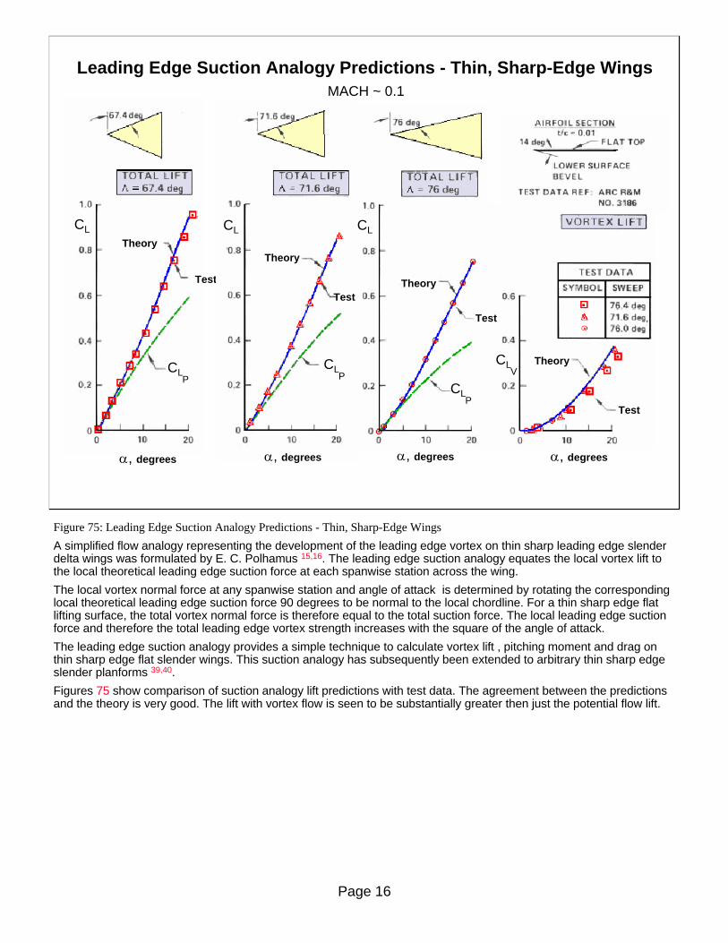
Figure 75: Leading Edge Suction Analogy Predictions - Thin, Sharp-Edge WingsA simplified flow analogy representing the development of the leading edge vortex on thin sharp leading edge slender delta wings was formulated by E. C. Polhamus 15,16. The leading edge suction analogy equates the local vortex lift to the local theoretical leading edge suction force at each spanwise station across the wing. The local vortex normal force at any spanwise station and angle of attack is determined by rotating the corresponding local theoretical leading edge suction force 90 degrees to be normal to the local chordline. For a thin sharp edge flat lifting surface, the total vortex normal force is therefore equal to the total suction force. The local leading edge suction force and therefore the total leading edge vortex strength increases with the square of the angle of attack.The leading edge suction analogy provides a simple technique to calculate vortex lift , pitching moment and drag on thin sharp edge flat slender wings. This suction analogy has subsequently been extended to arbitrary thin sharp edge slender planforms 39,40. Figures 75 show comparison of suction analogy lift predictions with test data. The agreement between the predictions and the theory is very good. The lift with vortex flow is seen to be substantially greater then just the potential flow lift.
Page 17
1.5
1.0
0.5
0.00 0.5 1.0
CL
ΔCDCL2
1.5
1.0
0.5
0.00 0.5 1.0
CL
ΔCDCL2
1.5
1.0
0.5
0.00 0.5 1.0
CL
ΔCDCL2
Mach ~ 0
1πAR
Zero Suction(No Vortex Lift)
Suction Analogy
Test Data
76O70O80O
Suction Analogy Drag Due to Lift Predictions
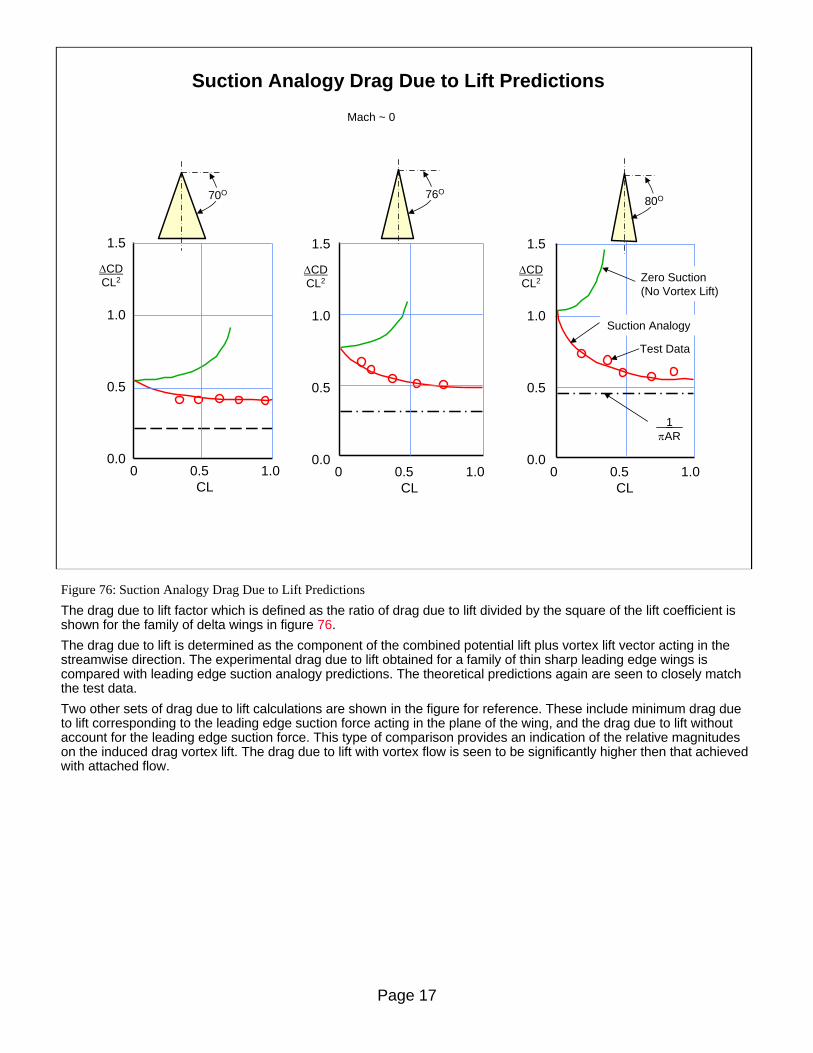
Figure 76: Suction Analogy Drag Due to Lift PredictionsThe drag due to lift factor which is defined as the ratio of drag due to lift divided by the square of the lift coefficient is shown for the family of delta wings in figure 76.The drag due to lift is determined as the component of the combined potential lift plus vortex lift vector acting in the streamwise direction. The experimental drag due to lift obtained for a family of thin sharp leading edge wings is compared with leading edge suction analogy predictions. The theoretical predictions again are seen to closely match the test data.Two other sets of drag due to lift calculations are shown in the figure for reference. These include minimum drag due to lift corresponding to the leading edge suction force acting in the plane of the wing, and the drag due to lift without account for the leading edge suction force. This type of comparison provides an indication of the relative magnitudes on the induced drag vortex lift. The drag due to lift with vortex flow is seen to be significantly higher then that achieved with attached flow.

Page 18
Mach Number Effects on Vortex Lift on a Thin Sharp Leading Edge Wing76O Delta Wing
Figure 77: Mach Number Effects on Vortex Lift on a Thin Sharp Leading Edge WingThrough the use of the suction analogy39, it has been shown that the development of vortex lift occurs also at supersonic speeds as long as the leading edge of the wing is swept behind the free stream Mach line and the planform subsequently has a subsonic leading edge. Figure 77 contains an example of predictions of vortex lift and drag due to lift at supersonic speeds along with the corresponding test data.

Page 19
NACA 66-009.3 NACA 0012
Thin Sharp Airfoil
Round Nose Airfoil
Effect of Airfoil Shape on Vortex Lift of a 76-deg Delta Wing
CT / CR = 0.125
Figure 78: Effect of Airfoil Shape on Vortex Lift of a 76-deg Delta WingThe leading edge suction analogy was extended to slender wings with round edges and thick sharp edges using a residual suction concept 10.With the residual section concept, the local leading edge suction force is compared with the local airfoil nose pressure drag force which acts in the plane of the wing. The round nose pressure force does not vary with angle of attack whereas the local leading edge suction force varies with the square of the angle of attack. Therefore, at some angle of attack, the magnitude of the suction force will equal and begin to exceed the local nose pressure drag force. This angle of attack is defined as the local separation angle of attack at which the leading edge vortex first starts to form at that station. The strength of the local leading edge vortex is then determined as the square of the difference between the actual angle of attack and the local separation angle of attack. This local vortex lift for a wing with a round leading edge, is therefore only a portion of the total local leading edge suction force. The difference between the total suction force and the portion converted into vortex lift is assumed to act in the local chord plane as a residual leading edge suction force.The residual suction method predicts the inboard movement of the leading edge vortex with angle of attack for slender wings with round nose airfoils or sharp edge wings with finite thickness, as well as the resulting lift, drag and pitching moment. Figure 78 shows lift predictions using the original thin sharp edge suction analogy theory and the extended round nose residual suction theory with test data for for two similar wing planforms. One wing had a thin sharp edge airfoil and the other wing had a thick round nose airfoil. The predictions agree well with the test data and illustrate the effect of the round nose in suppressing the leading edge vortex formation. The effect of the round nose is to reduce both the total wing lift and the corresponding wing drag to lift 10.The residual suction method was subsequently used to study the effects of airfoil shape, thickness distribution, wing camber and twist,flap deflections as well as planform variations on vortex flow 11.

Page 20
Comparison of Predicted and Measured Formation Vortex Boundaries• Mach = 0.85• Flat Symmetric Wing
71.2O
Predicted Start of Leading Edge Vortex @ Local Wing Station
Pressure Break
ΔCpL Before Pressure BreakΔCpL After Break
Typical Pressure Measurement Across The Span
at 2.5% Local Chord
ΔCpL = CpLOWER – CpUPPER at Same Station
Figure 79: Comparison of Predicted and Measured Formation Vortex BoundariesAn extensive series of wing tunnel tests were conducted as part of a joint NASA Langley / Boeing research effort 43,44
to provide an extensive database for use in validating theoretical aerodynamic and aeroelastic prediction theories. The wind tunnel model geometry consisted of an arrow wing plus body configurations including flat, twisted and cambered wings, as well as a variety of leading and trailing edge control surface deflections. The tests were conducted at subsonic, transonic and supersonic Mach numbers.The model geometry and a typical airfoil section are shown in figure 79 along with sample data obtained at Mach = 0.85 for the flat wing planform with a round nose airfoil.The variation of the lifting pressure coefficient at 2.5% local chord is shown for a typical spanwise station. The general characteristic of the pressures observed near the leading edge included a nearly linear variation of the lifting pressure coefficient with angle of attack up to an angle of attack where a break in the pressure curve would occur. As shown in the figure, the pressure break angle of attack at every spanwise station correlated very well with the theoretical prediction local separation angle which is defined as the angle of attack, αS, at a station at which the leading edge vortex first appears.The effect of the round nose airfoil is to create a range of angle of attack at which attached flow will be retained. For a flat symmetric wing, this region is symmetric for both positive and negative angles of attack.
Page 21
Effect of Flap Deflections on Leading Edge Vortex Development71.2O
Vary δF Across Span
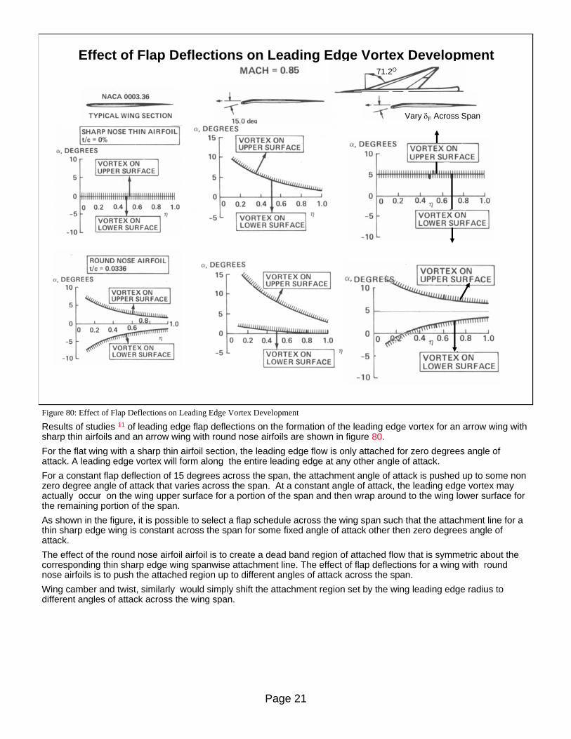
Figure 80: Effect of Flap Deflections on Leading Edge Vortex Development
Results of studies 11 of leading edge flap deflections on the formation of the leading edge vortex for an arrow wing with sharp thin airfoils and an arrow wing with round nose airfoils are shown in figure 80. For the flat wing with a sharp thin airfoil section, the leading edge flow is only attached for zero degrees angle of attack. A leading edge vortex will form along the entire leading edge at any other angle of attack. For a constant flap deflection of 15 degrees across the span, the attachment angle of attack is pushed up to some non zero degree angle of attack that varies across the span. At a constant angle of attack, the leading edge vortex may actually occur on the wing upper surface for a portion of the span and then wrap around to the wing lower surface for the remaining portion of the span.As shown in the figure, it is possible to select a flap schedule across the wing span such that the attachment line for a thin sharp edge wing is constant across the span for some fixed angle of attack other then zero degrees angle of attack.The effect of the round nose airfoil airfoil is to create a dead band region of attached flow that is symmetric about the corresponding thin sharp edge wing spanwise attachment line. The effect of flap deflections for a wing with round nose airfoils is to push the attached region up to different angles of attack across the span.Wing camber and twist, similarly would simply shift the attachment region set by the wing leading edge radius to different angles of attack across the wing span.
Page 22
Outboard Vortex WithNo Flap Deflection
Attached Flow WithOutboard Flap Deflection
Effect of Flap Deflections on Surface Streamlines
Mach ~ 0.90
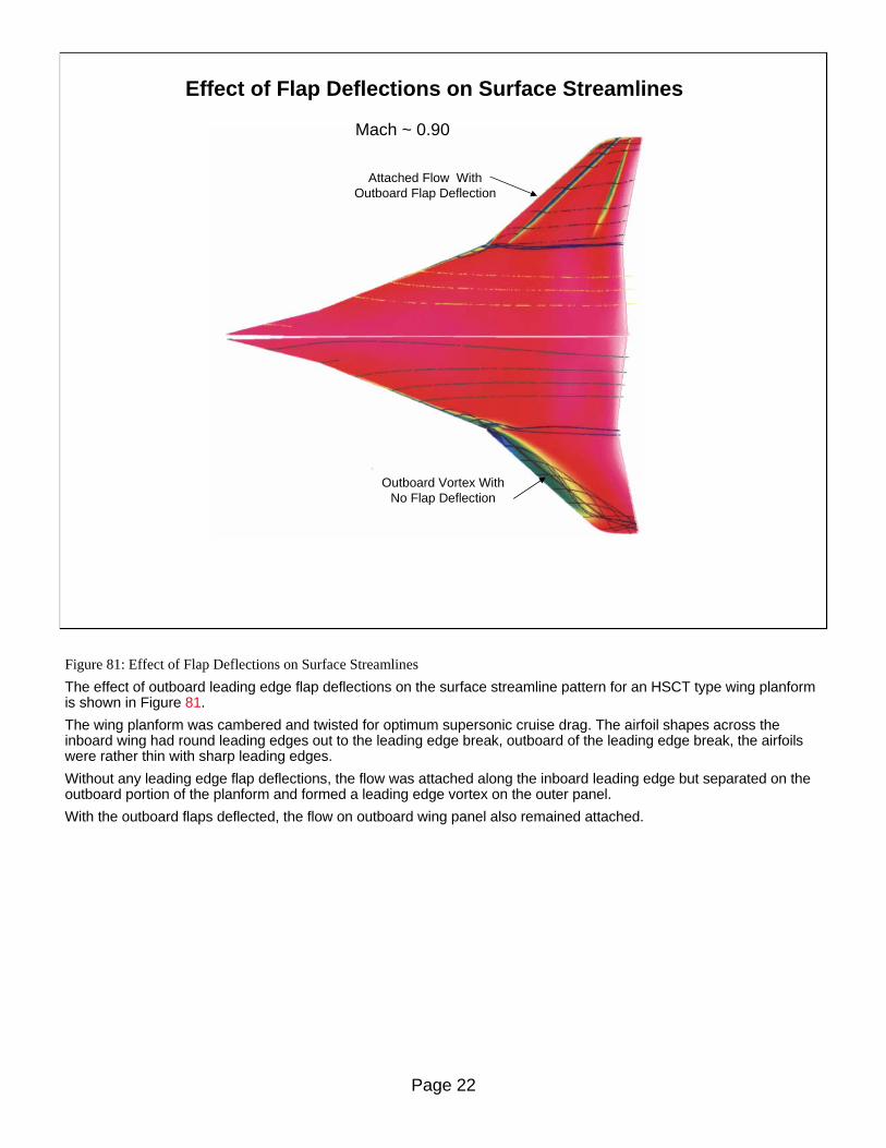
Figure 81: Effect of Flap Deflections on Surface StreamlinesThe effect of outboard leading edge flap deflections on the surface streamline pattern for an HSCT type wing planform is shown in Figure 81. The wing planform was cambered and twisted for optimum supersonic cruise drag. The airfoil shapes across the inboard wing had round leading edges out to the leading edge break, outboard of the leading edge break, the airfoils were rather thin with sharp leading edges.Without any leading edge flap deflections, the flow was attached along the inboard leading edge but separated on the outboard portion of the planform and formed a leading edge vortex on the outer panel.With the outboard flaps deflected, the flow on outboard wing panel also remained attached.

Page 23
-8
-6
-4
-2
0
2
4
6
8
0.0 0.1 0.2 0.3 0.4 0.5 0.6 0.7 0.8 0.9 1.02y/b
α deg
Attached Flow
Separated Flow
Leading Edge Vortex Development on an Arrow Wing At Mach = 1.7
0.090.200.350.500.650.800.93
2y/b
α deg
ΔCpL @ 2.5% Chord
-0.5
-0.4
-0.3
-0.2
-0.1
0.0
0.1
0.2
0.3
0.4
0.5
-8 -7 -6 -5 -4 -3 -2 -1 0 1 2 3 4 5 6 7 8
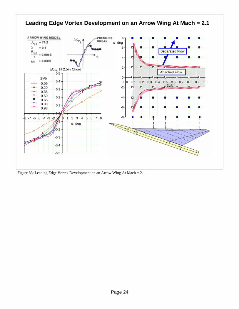
Figure 82: Leading Edge Vortex Development on an Arrow Wing At Mach = 1.7 Using the aforementioned approach of identifying the initial leading edge vortex formation at any spanwise station by the break in the lifting pressure variation with angle of attack, the separation boundaries for the swept arrow wing are shown for supersonic Mach numbers in Figures 82 and 82.Comparing these results with the corresponding subsonic separation boundary shown in Figure 79, indicates that the increased Mach numbers reduced the angle of attack range for attached flow. The general conditions leading to the formation and growth of a leading edge vortex at subsonic speeds are similar to those at supersonic speeds provided the leading edge is subsonic. Investigations of the effects of Reynolds number variations on leading edge vortices at subsonic speeds should, therefore, yield observations and conclusions that are applicable to similar supersonic flows.Consequently we will use results from of a number the experimental and computational of studies on the effects of Reynolds number variations on leading edge vortices at subsonic speeds, and develop conclusions that should be equally applicable to supersonic speeds..
Page 24
-8
-6
-4
-2
0
2
4
6
8
0.0 0.1 0.2 0.3 0.4 0.5 0.6 0.7 0.8 0.9 1.0
Attached Flow
Separated Flow
2y/b
α deg
-0.5
-0.4
-0.3
-0.2
-0.1
0.0
0.1
0.2
0.3
0.4
0.5
-8 -7 -6 -5 -4 -3 -2 -1 0 1 2 3 4 5 6 7 8
0.090.200.350.500.650.800.93
2y/b
ΔCpL @ 2.5% Chord
α deg
Leading Edge Vortex Development on an Arrow Wing At Mach = 2.1
Figure 83: Leading Edge Vortex Development on an Arrow Wing At Mach = 2.1

Page 25
Sharp Leading EdgeMach = 0.83Re = 6x10⁶
Spanwise Movement of the Leading Edge Vortex With Angle of Attack
0 2 4 6 8 10 12 14 16Angle of Attack deg
1.6
1.4
1.2
1.0
0.8
0.6
0.4
0.2
0.0
ΔCP
ΔCP @ 2y/b = 0.975
0.2 0.3 0.4 0.5 0.6 0.7 0.8 0.9 1.0Streamwise Station X/CR
14
12
10
8
6
4
2
0
α deg
X/CR = 0.60
X/CR = 0.95
X/CR = 0.80
X/CR = 0.40 Attached Flow
Vortex Flow
• Sharp Leading Edge• Small Radius• Medium Radius• Large Radius
Not to Scale
Figure 84: Spanwise Movement of the Leading Edge Vortex With Angle of AttackAn extensive wind tunnel test program 45 of a 65O delta wing model with interchangeable leading edges was conducted in the NASA Langley National Transonic Facility, NTF. The objective was to investigate the effects of Reynolds numbers and Mach number on slender-wing leading-edge vortex flow with four values of leading edge bluntness. Theexperimental data included surface pressure measurements, and measurements of normal force and pitching moment.The wing planform and various leading edge geometries are shown in figure 84.Measurements of the lifting pressures coefficients near the leading edge of the wing are shown in the figure for a typical wind tunnel Reynolds number. The attached flow boundary that was determined from the breaks in the lifting pressure coefficient curves, is also shown.The sharp edge wing apparently achieves attached flow over a small range of angle of attack because of the overall thickness of the wing and the rather steep angles of the sharp edge.

Page 26
Medium Round Leading EdgeMach = 0.85Re = 6x10⁶
0 2 4 6 8 10 12 14 16Angle of Attack deg
1.6
1.4
1.2
1.0
0.8
0.6
0.4
0.2
0.0
ΔCP
ΔCP @ 2y/b = 0.975
0.2 0.3 0.4 0.5 0.6 0.7 0.8 0.9 1.0Streamwise Station X/CR
14
12
10
8
6
4
2
0
α deg
Attached Flow
Vortex Flow
Spanwise Movement of the Leading Edge Vortex With Angle of Attack
X/CR = 0.60
X/CR = 0.95
X/CR = 0.80
X/CR = 0.40
Figure 85: Spanwise Movement of the Leading Edge Vortex With Angle of Attack
Similar pressure measurements for the medium round nose geometry are shown in figure 85 for the same test conditions. The separation boundary determined for this geometry is also shown.

Page 27
Mach ~ 0.83 to 0.85Leading Edge Radius Effect on Inboard Movement of the Leading Edge Vortex
Airfoil Closure Region
14
12
10
8
6
4
2
0
α deg
Stream Wise Station X/CR0.2 0.3 0.4 0.5 0.6 0.7 0.8 0.9 1.0
Attached Flow
Vortex FlowAttached Flow
Vortex Flow
Medium Round Leading Edge
Sharp Leading Edge
Figure 86: Leading Edge Radius Effect on Inboard Movement of the Leading Edge VortexThe separation boundaries for the sharp leading edge and the medium leading edge geometries are compared in figure 86 The medium round nose geometry is seen to provide approximately and additional 4 degrees angle of attack over which attached flow is retained.

Page 28
0 2 4 6 8 10 12 14 16Angle of Attack deg
1.6
1.4
1.2
1.0
0.8
0.6
0.4
0.2
0.0
ΔCP
0.2 0.3 0.4 0.5 0.6 0.7 0.8 0.9 1.0Streamwise Station X/CR
14
12
10
8
6
4
2
0
α deg
ΔCP @ 2y/b = 0.975
X/CR = 0.95
X/CR = 0.80
X/CR = 0.60
X/CR = 0.40
Medium Round Leading EdgeMach = 0.85Re = 24x106
Attached Flow
Vortex Flow
Spanwise Movement of the Leading Edge Vortex With Angle of Attack
Figure 87: Spanwise Movement of the Leading Edge Vortex With Angle of Attack – Re = 24 x 106
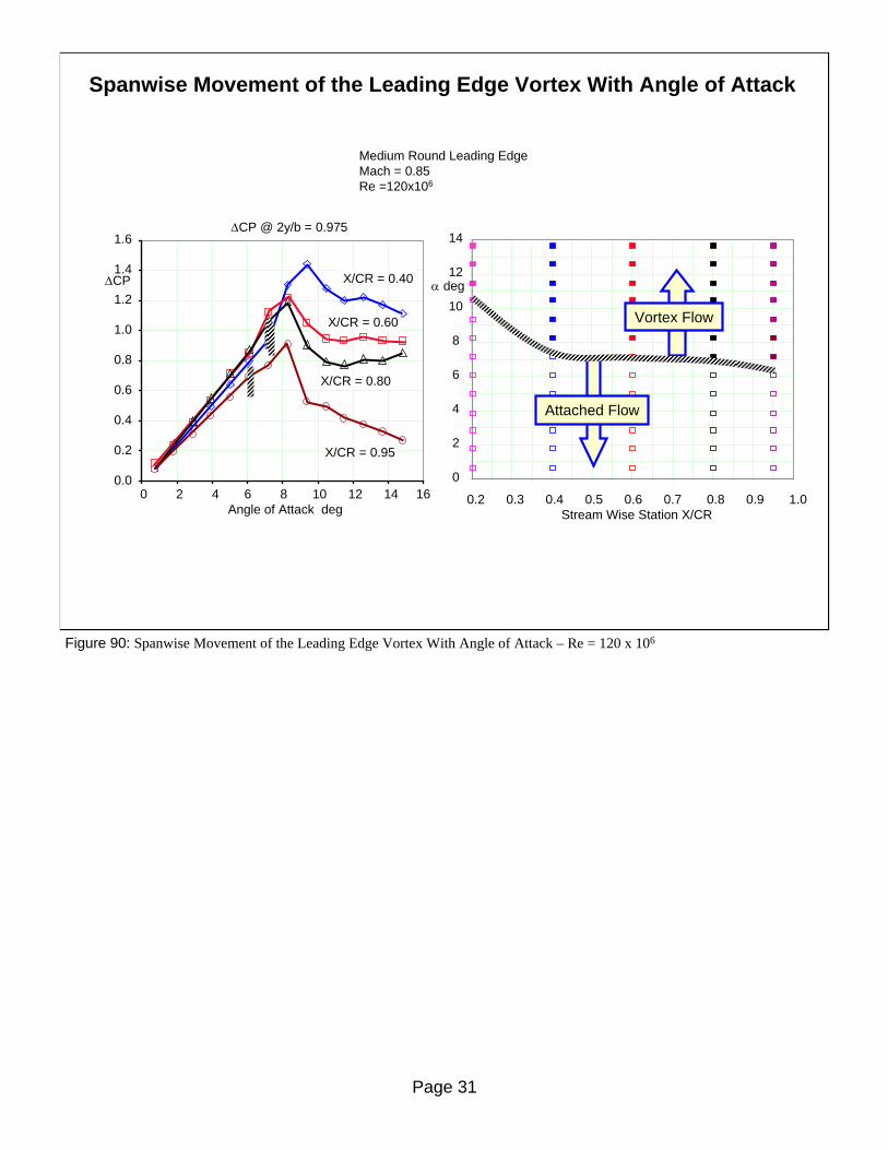
Experimental results obtained with the medium nose radius geometry are shown in figures 87 through 90 for increasing Reynolds number from typical wind tunnel conditions to approximately full scale conditions.The set of lifting pressure curves for each of the test Reynolds numbers, all show the same general characteristic trends with angle of attack. The lifting pressures measures near the leading edge across the wing span all vary linearly with angle of attack up to some departure angle corresponding to a break in the lifting pressure curve. These departure angles were used to define the spanwise angle of attack range for attached flow and thereby define the inboard movement of the origin of the leading edge vortex with angle of attack.

Page 29
0 2 4 6 8 10 12 14 16Angle of Attack deg
1.6
1.4
1.2
1.0
0.8
0.6
0.4
0.2
0.0
ΔCP
ΔCP @ 2y/b = 0.975
X/CR = 0.95
X/CR = 0.80
X/CR = 0.60
X/CR = 0.40
Medium Round Leading EdgeMach = 0.85Re = 48x106
0.2 0.3 0.4 0.5 0.6 0.7 0.8 0.9 1.0Streamwise Station X/CR
14
12
10
8
6
4
2
0
α deg
Attached Flow
Vortex Flow
Spanwise Movement of the Leading Edge Vortex With Angle of Attack
Figure 88: Spanwise Movement of the Leading Edge Vortex With Angle of Attack – Re = 48 x 106

Page 30
0 2 4 6 8 10 12 14 16Angle of Attack deg
1.6
1.4
1.2
1.0
0.8
0.6
0.4
0.2
0.0
ΔCP
Medium Round Leading EdgeMach = 0.85Re =96x106
ΔCP @ 2y/b = 0.975
X/CR = 0.95
X/CR = 0.80
X/CR = 0.60
X/CR = 0.40
0.2 0.3 0.4 0.5 0.6 0.7 0.8 0.9 1.0Stream Wise Station X/CR
14
12
10
8
6
4
2
0
α deg
Attached Flow
Vortex Flow
Spanwise Movement of the Leading Edge Vortex With Angle of Attack
Figure 89: Spanwise Movement of the Leading Edge Vortex With Angle of Attack – Re = 96 x 106
Page 31
0 2 4 6 8 10 12 14 16Angle of Attack deg
1.6
1.4
1.2
1.0
0.8
0.6
0.4
0.2
0.0
ΔCP
Medium Round Leading EdgeMach = 0.85Re =120x106
ΔCP @ 2y/b = 0.975
X/CR = 0.95
X/CR = 0.80
X/CR = 0.60
X/CR = 0.40
0.2 0.3 0.4 0.5 0.6 0.7 0.8 0.9 1.0Stream Wise Station X/CR
14
12
10
8
6
4
2
0
α deg
Spanwise Movement of the Leading Edge Vortex With Angle of Attack
Attached Flow
Vortex Flow
Figure 90: Spanwise Movement of the Leading Edge Vortex With Angle of Attack – Re = 120 x 106
Page 32
Medium Round Leading EdgeMach = 0.85
Reynolds Number Effect on Inboard Movement of the Leading Edge Vortex
14
12
10
8
6
4
2
0
α deg
24 x 106 and 48 x 106
6 x 10⁶ , 96 x 106 and 120 x 106
Airfoil Closure Region
Stream Wise Station X/CR0.2 0.3 0.4 0.5 0.6 0.7 0.8 0.9 1.0
Vortex Flow
Attached Flow
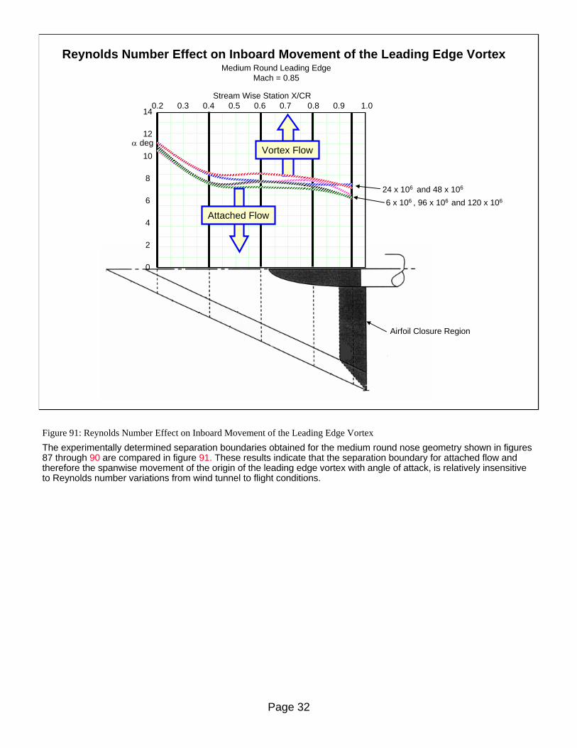
Figure 91: Reynolds Number Effect on Inboard Movement of the Leading Edge VortexThe experimentally determined separation boundaries obtained for the medium round nose geometry shown in figures 87 through 90 are compared in figure 91. These results indicate that the separation boundary for attached flow and therefore the spanwise movement of the origin of the leading edge vortex with angle of attack, is relatively insensitive to Reynolds number variations from wind tunnel to flight conditions.

Page 33
0 4 8 12 16 20 24 28Angle of Attack deg
Angle of Attack deg 0 4 8 12 16 20 24 28
1.4
1.2
1.0
0.8
0.6
0.4
0.2
0.0
CL.10
.05
0.0
-.05
-.10
-.15
-.20
-.25
-.30
-.35
-.40
CM
Medium Round Leading EdgeMach = 0.85Re = 6x10⁶ to 120 x 106
Effect of Reynolds Number on Lift and Pitching Moment for a 65O Delta Wing
Figure 92: Effect of Reynolds Number on Lift and Pitching Moment for a 65O Delta WingFigure 92 shows the variation of normal force and pitching moment with angle of attack for the NASA 65O delta wing. The data shown in the figure also correspond to the number of Reynolds numbers from wind tunnel to flight conditions. The lift and the pitching moment show little effect for the variations of Reynolds numbers.

Page 34
Two-Dimensional Crossflow Plane Potential Flow Analyses Methods
Figure 93: Two-Dimensional Crossflow Plane Potential Flow Analyses MethodsTheoretical Analyses of Leading Edge Vortex Flows
The detailed characteristics of the flow field associated with leading edge vortices are indeed very complicated. The formation of the leading edge vortex is in itself a viscous related phenomena since boundary layer separation from the surface of a wing is the basic origin of the leading edge vortex. The leading edge vortex once formed, forms a highly concentrated region of vorticity that decays relatively slowly downstream and consequently, behaves very much like a inviscid potential flow phenomena. The inviscid like nature of the developed vortex flows allowed the development of early potential flow computational models that captured some of the characteristics of leading edge vortices and their effects10,. Some of the earliest analytical models included the two-dimensional cross flow models as shown in figure 93.

Page 35
Three Dimensional Potential Flow Analysis Models of Leading Edge Vortex Flow Thin Sharp Edge Highly Swept Wings
Figure 94: Three Dimensional Potential Flow Analysis Models of Leading Edge Vortex Flow The earliest crossflow leading edge vortex models were followed by that represented the complete three dimensional vortex by either a series of discrete vortices of by a complete three dimensional modeling of the vortex sheet as shown in figure 94. These simplified representation of the leading edge vortex lead to reasonably good correlations with test data for thin sharp edge wings as shown in the figure.More recently, numerical solutions to the Euler equations have led to useful numerical computations of the flow characteristics of leading edge vortices on thin sharp edge wings. In this care, the numerical viscosity in the solution process of the Euler equations, no matter how small, is sufficient to result in the formation and growth of the leading edge vortices.

Page 36
Comparison of Experimental and Euler Predicted Pressures on a 75O Delta Wing
Figure 95: Comparison of Experimental and Euler Predicted Pressures on a 75O Delta WingFigure 95 contains comparisons of Euler spanwise pressure predictions with experiment17 at supersonic speeds for a thin sharp 75O delta wing at an angle of attack of 12O. At both analysis Mach numbers, the experimental data and the theoretical predictions indicate leading edge separation that resulted in the formation of a leading edge vortex on the upper surface. The most notable difference between the Euler predictions and the experimental data is the lack of a secondary vortex in the Euler predictions. The secondary vortex is a local viscous phenomena which can not be predicted with the an inviscid code. At the lower Mach number, Mach 1.7, The effect of the secondary vortex results in two local pressure peaks. At the higher Mach number, Mach 2.8, The secondary vortex appears to have little effect on the pressure distributions. It appears that the effect of the secondary vortex vanishes with increasing Mach Number.

Page 37
CL CL
Experimental and Euler Results for a Thin Sharp Flat Delta Wing in YawSweep = 75O
α = 12O
β = 8O
Figure 96: Experimental and Euler Results for a Thin Sharp Flat Delta Wing in Yaw
Theoretical and experimental results for the flat wing at 12O degrees angle of attack and for 8O of yaw are shown in figure 96 for Mach 1.7 and 2.8. The pressure distributions and flow field features are shown for both the windward (left) side and the leeward (right) side.For both cases the asymmetry of the flow due to yaw is evident although the flow fields are quite different for the two Mach numbers. At the lower Mach number, leading edge separation occurred on both the windward and leeward edges. The windward edge separation developed into a separation bubble that lies close to the wing surface. The leeward side separation developed into a conventional leading edge vortex.At the higher Mach number, The flow is attached on the windward side and develops a leading edge vortex on the leeward side. The asymmetry in flow fields for both Mach numbers leads to rolling moment due to the yaw condition.For both of the Mach numbers, the Euler predictions agree quite well with the experimental results.
Page 38
Comparisons of Euler and Navier Stokes Solution65o Cropped Delta Wing Mach Mach = 0.85 α = 10o
EULER SOLUTION NAVIER STOKES SOLUTION
Pathlines
Wing Isobars
Total Pressure ContoursX/Cr = 0.8
Vorticity ContoursX/Cr = 0.8
ΔCP = 0.1
ΔCPT = 0.05
Δ| rot v | = 0.0001
Origin of Leading Edge Vortex
Origin of Leading Edge Vortex
Primary Vortex Primary Vortex
Secondary Vortex Secondary Vortex
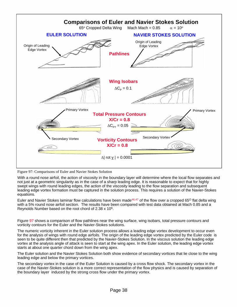
Figure 97: Comparisons of Euler and Navier Stokes SolutionWith a round nose airfoil, the action of viscosity in the boundary layer will determine where the local flow separates and not just at a geometric singularity as in the case of a sharp leading edge. It is reasonable to expect that for highly swept wings with round leading edges, the action of the viscosity leading to the flow separation and subsequent leading edge vortex formation must be captured in the solution process. This requires a solution of the Navier-Stokes equations.Euler and Navier Stokes laminar flow calculations have been made46,47 of the flow over a cropped 65O flat delta wing with a 5% round nose airfoil section. The results have been compared with test data obtained at Mach 0.85 and a Reynolds Number based on the root chord of 2.38 x 10⁶.
Figure 97 shows a comparison of flow pathlines near the wing surface, wing isobars, total pressure contours and vorticity contours for the Euler and the Navier-Stokes solutions.The numeric vorticity inherent in the Euler solution process allows a leading edge vortex development to occur even for the analysis of wings with round edge airfoils. The origin of the leading edge vortex predicted by the Euler code is seen to be quite different then that predicted by the Navier-Stokes Solution. In the viscous solution the leading edge vortex at the analysis angle of attack is seen to start at the wing apex. In the Euler solution, the leading edge vortex starts at about one quarter chord down from the wing apex.The Euler solution and the Navier Stokes Solution both show evidence of secondary vortices that lie close to the wing leading edge and below the primary vortices. The secondary vortex in the case of the Euler Solution is caused by a cross flow shock. The secondary vortex in the case of the Navier-Stokes solution is a more correct representation of the flow physics and is caused by separation of the boundary layer induced by the strong cross flow under the primary vortex.

Page 39
Comparisons of Euler and Navier-Stokes Laminar Flow Results65o Cropped Delta Wing Mach = 0.85
Rec = 1.28 x 10⁶ α = 10O
0.0 0.2 0.4 0.6 0.8 1.0η = y/s
-1.6
-1.2
-0.8
-0.4
0.0
0.4
CP
0.0 0.2 0.4 0.6 0.8 1.0η = y/s
-1.6
-1.2
-0.8
-0.4
0.0
0.4
CP
0.0 0.2 0.4 0.6 0.8 1.0η = y/s
-1.6
-1.2
-0.8
-0.4
0.0
0.4
CPX/CR = 0.3
X/CR = 0.6 X/CR = 0.8
65O
λ = 0.15
Round Nose Airfoil:T/C mac = 5 %LE radius = 0.7%
Test DataNavier-Stokes ( Laminar)Euler
Figure 98: Comparisons of Euler and Navier-Stokes Laminar Flow ResultsFigure 98 provides some insight into the differences that might be encountered when applying an Euler code for prediction the flow characteristics on a highly swept round nose airfoil. The figure includes a comparison of the wing pressures calculated by an Euler analyses and a Navier-Stokes analyses46, with test data obtained at Mach 0.85 and a Reynolds Number based on the root chord of 2.38 x 10⁶.The Navier-Stokes predictions appear to predict the location of the primary vortex and the minimum induced pressures quite well. The overall Navier-Stokes predictions agree much better with the test data then do the Euler code predictions. These Navier-Stokes predictions however, did not appear to properly capture the details of the secondary vortex interactions which occur in the region close to the leading edge. This is evident by the differences in the predicted and measured upper surface pressures near the wing leading edge in this figure.

Page 40
Effect of Reynolds Number on Computed Surface Streamlines Mach = 0.85CFL3D Spalart-Allmaras Turbulence Model Round Leading Edge
65O
α = 16.37O Rn = 6 x 10⁶ α = 16.44O Rn = 48 x 106
α = 16.38O Rn = 84 x 106 α = 16.59O Rn = 120 x 106
A
A
Primary Leading Edge Vortex
Secondary Vortex
Trailing Edge Separation
Figure 99: Effect of Reynolds Number on Computed Surface Streamlines Mach = 0.85An extensive computational study48 was conducted in which the CFL3D Navier-Stokes code was used with the Spalart-Allmaras turbulence model to predict the flow characteristics of the 65O delta wing with the medium leading edge radius and the round leading edge radius that were previously discussed, (figures 84 through 92). The analyses were made for Mach = 0.85 and a range of Reynolds numbers from wind tunnel to full scale flight conditions. Calculated surface streamlines are shown in figure 99. The predicted streamlines are essential identical for the compute Reynolds number range of 6 x 10⁶ to 120 x 106. The surface stream lines clearly show the primary leading edge vortex, the induced secondary vortex and separation near the wing trailing where the thickness rapidly closed to the sharp edge.
Page 41
CFL3D Turbulent Flow AnalysesMach = 0.85 Rn = 6x10⁶
Round Leading Edge Geometry
Comparison of Predicted and Measured Spanwise Pressure Distributions
Attached Flow Condition α = 7.14O
Separated Flow Condition α = 12.28O
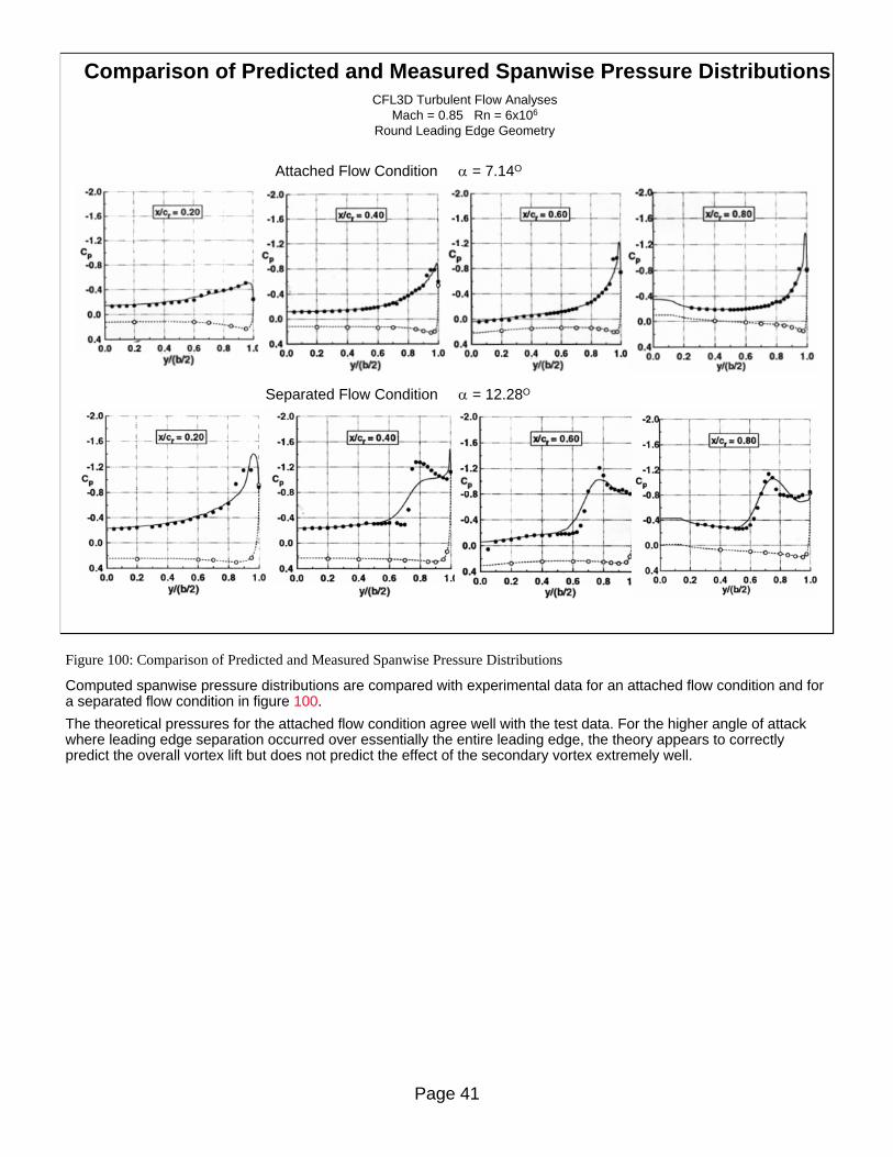
Figure 100: Comparison of Predicted and Measured Spanwise Pressure Distributions
Computed spanwise pressure distributions are compared with experimental data for an attached flow condition and for a separated flow condition in figure 100.The theoretical pressures for the attached flow condition agree well with the test data. For the higher angle of attack where leading edge separation occurred over essentially the entire leading edge, the theory appears to correctly predict the overall vortex lift but does not predict the effect of the secondary vortex extremely well.

Page 42
CFL3D Predictions Wind Tunnel Data
Comparisons of Predicted Reynolds Number Effects on Cp with Test Data65O Flat Delta Wing With Round Leading Edge
Mach = 0.85 α ~ 7O
Figure 101: Comparisons of Predicted Reynolds Number Effects on Cp with Test DataExperimental and theoretical pressure distributions for an angle of attack of 7O where the flow remains attached are shown in figure 101 for the Reynolds number range of wind tunnel to flight. Both theory and experiment indicate that the pressure distributions in flight are the same at a typical wind tunnel Reynolds number.
Page 43
CFL3D Predictions Wind Tunnel Data
Comparisons of Predicted Reynolds Number Effects on Cp with Test Data65O Flat Delta Wing With Round Leading Edge
Mach = 0.85 α ~ 12O
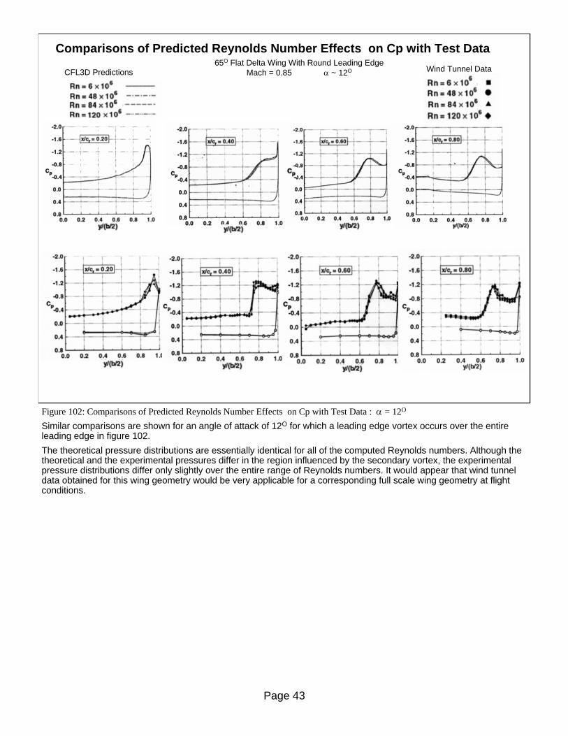
Figure 102: Comparisons of Predicted Reynolds Number Effects on Cp with Test Data : α = 12O
Similar comparisons are shown for an angle of attack of 12O for which a leading edge vortex occurs over the entire leading edge in figure 102.The theoretical pressure distributions are essentially identical for all of the computed Reynolds numbers. Although the theoretical and the experimental pressures differ in the region influenced by the secondary vortex, the experimental pressure distributions differ only slightly over the entire range of Reynolds numbers. It would appear that wind tunnel data obtained for this wing geometry would be very applicable for a corresponding full scale wing geometry at flight conditions.

Page 44
-.40
-.35
-.30
-.25
-.20
-.15
-.10
-.05
.000 .1 .2 .3 .4 .5 .6 .7 .8 .9 1.
Semi Span Station η = 2y/b
CP
-.40
-.35
-.30
-.25
-.20
-.15
-.10
-.05
.000 .1 .2 .3 .4 .5 .6 .7 .8 .9 1.
Semi Span Station η = 2y/b
CP
(Blunt)
The Effect of Leading Edge Radius on Upper Surface Pressures
• CFL3D Results• 65O Flat Delta Wing• Mach = 1.60• Re = 106
• Turbulent Flow Model
α = 4 deg α = 8 deg
Figure 103 : The Effect of Leading Edge Radius on Upper Surface PressuresResults of a Navier-Stokes parametric computational study49 that was conducted to investigate the effects of leading edge radius, leading edge camber, Reynolds number and boundary layer model on the flow characteristics of a 65O
delta wing at Mach = 1.6 are shown in figures 103 through 106. Analyses were made for two different angles of attack that included 4O and 8O. The smaller angle of attack, according to the leading edge vortex formation boundary shown in figure 10, should result in attached flow even for the sharp leading edge geometry. At the larger angle of attack, a leading edge vortex is expected to occur. Figure 103 shows results of the Navier-Stokes analyses for various leading edge geometries at the two angles of attack. The leading edge geometries included a sharp edge, an elliptic nose geometry and a blunt round nose geometry.At 4 degrees angle of attack, the pressure distribution on the sharp nose geometry shows a slight inflection that corresponds to a leading edge separation bubble. Both round nose geometries had attached flow at the lower angle of attack.At 8 degrees angle of attack, leading edge vortex flow occurred on all three geometries. It does appear that the round nose geometries did result in a reduction in the vortex lift which indicates that the formation of the leading edge vortex was indeed delayed.

Page 45
Effect of Camber -Turbulent Flow Model-.50
-.45
-.40
-.35
-.30
-.25
-.20
-.15
-.10
-.05
.000 .1 .2 .3 .4 .5 .6 .7 .8 .9 1.
Semi Span Station η = 2y/b
CP
αC = 10.0O
αC = 8.0O
αC = 4.0O
αC = 0.0O
The Effect of Leading Edge Camber on Upper Surface PressuresCFL3D Results65O Flat Delta WingMach = 1.60α = 8 degRe = 106
Camber Variations – Medium nose Radius ( 20:1 Ellipse)
Figure 104: The Effect of Leading Edge Camber on Upper Surface Pressures
The effect of increasing leading edge camber with the medium nose radius elliptic geometry was analyzed at an angle of attack of 8 degrees with Navier-Stokes turbulent flow analyses. The results as shown in figure 104, indicate that increased nose camber can be effective in delaying the formation of the leading edge vortex. The results are consistent with the explanation on the benefits of leading edge radius and nose camber as offered by the residual suction analogy in conjunction with figure 80. The leading edge radius creates a region of angle of attack for which the flow remains attached and the effect of nose down camber is to shift the region of attached flow to higher angles of attack.The 4O camber shown in figure 104 was not sufficient to delay the leading edge vortex formation. The 8O degree camber shifted the attached flow region such that a leading edge separation just started to form. The largest camber resulted in attached flow at the analysis station.

Page 46
Re = 1.0 x 10⁶
Re = 2.0 x 10⁶
Re = 5.0 x 10⁶
-.45
-.40
-.35
-.30
-.25
-.20
-.15
-.10
-.05
.000 .1 .2 .3 .4 .5 .6 .7 .8 .9 1.
Semi Span Station η = 2y/b
CP
Uncambered Elliptic Nose airfoil
0 .1 .2 .3 .4 .5 .6 .7 .8 .9 1.
Semi Span Station η = 2y/b
-.50
-.45
-.40
-.35
-.30
-.25
-.20
-.15
-.10
-.05
.00
CP
Cambered Elliptic Nose airfoil αC = 10O
The Effect of Reynolds Number on Upper Surface PressuresCFL3D Results65O Flat Delta WingMach = 1.60α = 8 degTurbulent Flow Model
Figure 105: The Effect of Reynolds Number on Upper Surface PressuresThe effect of a moderate increase in Reynolds number on the elliptic nose configurations with and without nose camber, was also analyzed with the turbulent flow model. The computed pressure distributions are shown in figure 105 for 8O angle of attack. The results for the uncambered wing where the leading edge separation occurs, imply that increasing the Reynolds number slightly did not affect the formation of the leading edge vortex. The minimum pressure peak on the wing, however, did increase.The flow on the cambered wing was an attached flow case The overall effect of the Reynolds number increase for this attached flow case was also rather small. The increase in Reynolds number appears to have resulted in a slight separation at the base of the recompression that occurred near the leading edge as evidenced by the slight inflection in the pressure curves.
Page 47
The Effect of Laminar Flow Versus Turbulent Flow on Upper Surface Pressures
αC = 10.0O
-.50
-.45
-.40
-.35
-.30
-.25
-.20
-.15
-.10
-.05
.000 .1 .2 .3 .4 .5 .6 .7 .8 .9 1.
Semi Span Station η = 2y/b
CP
Laminar Flow Model
Turbulent Flow Model
CFL3D Results65O Flat Delta WingMedium Leading Edge RadiusMach = 1.60α = 8 degRe = 106
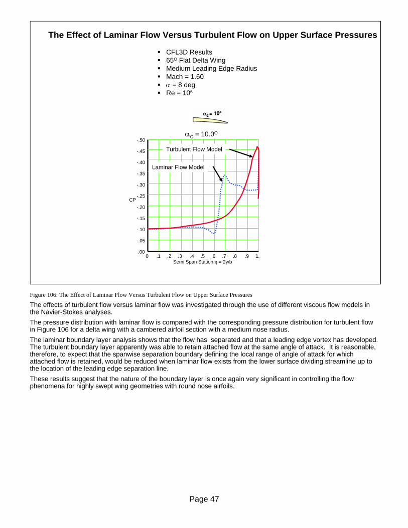
Figure 106: The Effect of Laminar Flow Versus Turbulent Flow on Upper Surface Pressures
The effects of turbulent flow versus laminar flow was investigated through the use of different viscous flow models in the Navier-Stokes analyses. The pressure distribution with laminar flow is compared with the corresponding pressure distribution for turbulent flow in Figure 106 for a delta wing with a cambered airfoil section with a medium nose radius. The laminar boundary layer analysis shows that the flow has separated and that a leading edge vortex has developed. The turbulent boundary layer apparently was able to retain attached flow at the same angle of attack. It is reasonable, therefore, to expect that the spanwise separation boundary defining the local range of angle of attack for which attached flow is retained, would be reduced when laminar flow exists from the lower surface dividing streamline up to the location of the leading edge separation line.These results suggest that the nature of the boundary layer is once again very significant in controlling the flow phenomena for highly swept wing geometries with round nose airfoils.
Page 48
The Effect of Laminar Flow Versus Turbulent Flow on Upper Surface Pressures
Turbulent FlowLaminar Flow
ARC3D 75O Flat Delta WingSharp Thin Leading EdgeMach = 1.95α = 20 degRe = 4.48 x 10⁶
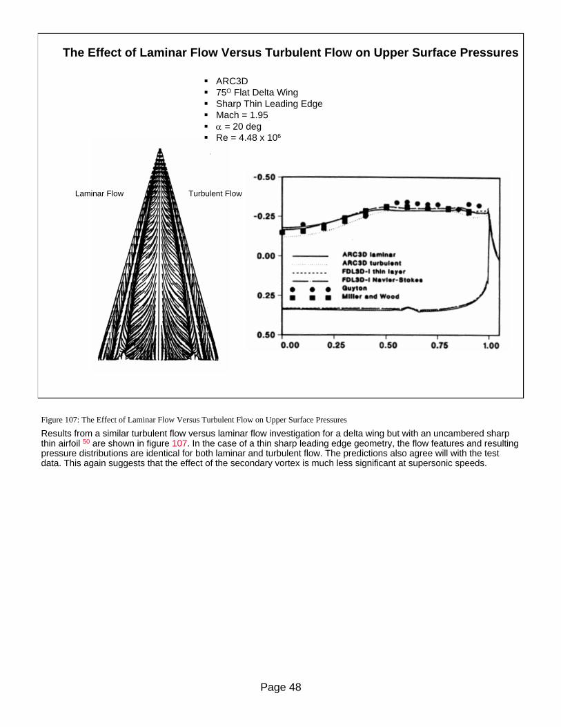
Figure 107: The Effect of Laminar Flow Versus Turbulent Flow on Upper Surface Pressures
Results from a similar turbulent flow versus laminar flow investigation for a delta wing but with an uncambered sharp thin airfoil 50 are shown in figure 107. In the case of a thin sharp leading edge geometry, the flow features and resulting pressure distributions are identical for both laminar and turbulent flow. The predictions also agree will with the test data. This again suggests that the effect of the secondary vortex is much less significant at supersonic speeds.

Page 49
ΛLE
0.0 -.01 -.02 -.03 -.04 -.05CM
1.0
0.9
0.8
0.7
0.6
0.5
0.4
0.3
0.2
0.1
0.0
CL
.01 0.0 -.02 -.04 -.06CM
1.0
0.9
0.8
0.7
0.6
0.5
0.4
0.3
0.2
0.1
0.0
CL50O
60O
70O
Planform Effects on Pitching Moment• Subsonic Speeds• Wind Tunnel Reynolds Number
ΛLE = 75O
Figure 108: Planform Effects on Pitching Moment
Figure 108 contains experimental pitching moment curves for a number of different wing planforms but having common airfoil geometry. Although the general conclusions about the leading edge vortices as previously discussed are applicable to these various planforms, the impact on the resulting aerodynamic characteristics can be quite different even for the simple case of wings with straight leading edges. However using the clues offered by the simple flow analogies it is possible to explain possible effects associated with wing planform modifications.The effect of the reduced sweep for delta wing planforms is shown to destabilizing in figure 108. As shown in figure 75 the total vortex lift does not vary significantly with wing sweep. The vortex lift essentially grows linearly from the wing root to the wing tip. Therefore, moment arm for the vortex lift on the higher swept wing is greater and thereby produces a more stabilizing nose down moment.Similarly, notching the trailing edge was also found to be destabilizing even though the leading edge vortex would be essentially the same for all the planforms. In this case as the angle of attack increased, some of the stabilizing vortex lift is lost where the wing trailing area has been removed.

Page 50
-5.0 0.0 5.0 10.0 15.0 20.0 25.0 30.0Angle of Attack deg
2.0
1.8
1.6
1.4
1.2
1.0
0.8
0.6
0.4
0.2
0.0
-.2
-.4
CL
α = 18O
α = 0O
α = 0O
α = 6O
α = 6O
α = 12O
α = 18O
α = 12O
Lift Curves and Flow CharacteristicsMach ~ 0.1
Figure 109: Wing Strake Effects on Lift and Wing Flow CharacteristicsThe current concepts for HSCT type configuration typically incorporate a double delta wing planform. These planforms have a highly swept inboard wing panel with round nose airfoils and a reduced sweep outer wing panel with sharp thin airfoils to provide a balance between the desire for slender wing geometry for supersonic cruise performance and increased span for low speed high lift performance.The flow over these wings at the design condition is well behaved attached flow. At off design conditions leading edge vortices may develop on the strake. The strake vortex flowing aft can have a significant effect on the outer wing panel. The flow at supersonic conditions is not too dissimilar then that at subsonic conditions. Some insight can be gained by examining results obtained initially obtained at subsonic speeds.The variation of lift and pitching moment with angle of attack for a wing-body combination with and without a strake at low speeds is shown in Figure 109. The wing and the strake both had thin airfoil sections with sharp leading edges.This figure illustrates four types of flow characteristics that have been observed51 on Wing/Strake Configurations at subsonic conditions. These include: 1. Completely attached flow, 2. Coexistence of a strake vortex and attached flow, 3. Coexistence of of a strake vortex with a bubble vortex and 4. Strake vortex breakdown.At close to zero degrees of attach, the flow is attached over both wings. The lift and pitching moment curves are linear in this region. The addition of the strake results in a forward movement of the aerodynamic center. As the angle of attach is increased to 6 degrees The wing without the strake is seen to have attached flow over most of the wing surface except in a region near the wing tip as the tip vortex develops and in a region very close to the leading edge where a very small leading edge bubble formed due to the leading edge separation that has reattached on the surface and has not formed a leading edge vortex due to the low sweep on the outer panel. The wing with strake shows similar flow on the outboard wing panel along with the existence of a strake vortex and a “kink” vortex. The strake vortex formed on the sharp edge strake leading edge and rolled up into a spiral vortex over the wing. The kink vortex is associated with the discontinuity in the wing leading edge. The strake vortex is fed by separated leading edge flow on the strake flow up to the intersection with the wing. Beyond the wing leading edge, the strake vortex persists down stream under its own energy. The wing pitching moment shows a slight aft movement in the aerodynamic center. The wing with strake has increased lift and more nose up lifting moment that the wing due to the vortex lift on the strake.As the angle of attack is increased to 12 degrees, the wing flow pattern consists of a small region of separated flow near the leading edge, a large bubble vortex, a region of attached flow behind the bubble vortex and the tip edge vortex region. This results in both a reduced lift curve slope and a further aft movement on the aerodynamic center. The strake wing shows stronger strake and kink vortices that tend to compress the bubble vortex on the wing. This results in a significant increase in lift and increased in nose up pitching moment.At the highest angle of attack The isolated wing flow is completely separated, the wing is stalled and starts to encounter pitchup. The wing-strake lift curve decreases and a sudden nose up pitching moment appears due to the breakdown of the strake vortex near the wing trailing edge.

Page 51
Comparison of Wind Tunnel and Flight Observed Flow Development 12O Angle of Attack
F-16
YF-17
Figure 110: Comparison of Wind Tunnel and Flight Observed Flow DevelopmentFigure 110 shows a comparison wind tunnel and flight test observed flow development on a straked wing at 8 degrees angle of attack. The complex flow patterns obtained in the wind tunnel and on the airplane are essentially identical.
Page 52
Effect of Mach Number on Lift and Pitching Moment
1.6
1.4
1.2
1.0
0.8
0.6
0.4
0.2
0.0
1.6
1.4
1.2
1.0
0.8
0.6
0.4
0.2
0.0
0 4 8 12 16 20 24 28Angle of Attack, deg
.20 .10 0.0 -.10 -.20 -.30Pitching Moment
CN
CN
Mach = 1.2
76O
76O
1.6
1.4
1.2
1.0
0.8
0.6
0.4
0.2
0.0
1.6
1.4
1.2
1.0
0.8
0.6
0.4
0.2
0.0
0 4 8 12 16 20 24 28Angle of Attack, deg
CN
CN
.20 .10 0.0 -.10 -.20Pitching Moment
Mach = 0.8
76O
76O
30O
30O
30O
30O
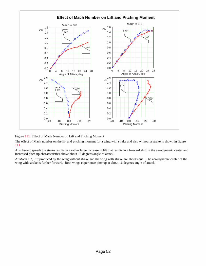
Figure 111: Effect of Mach Number on Lift and Pitching MomentThe effect of Mach number on the lift and pitching moment for a wing with strake and also without a strake is shown in figure 111. At subsonic speeds the strake results in a rather large increase in lift that results in a forward shift in the aerodynamic center and increased pitch up characteristics above about 16 degrees angle of attack.At Mach 1.2, lift produced by the wing without strake and the wing with strake are about equal. The aerodynamic center of the wing with strake is further forward. Both wings experience pitchup at about 16 degrees angle of attack.

Page 53
Effect of Mach Number on Flow Patterns, αM = 10 deg.
Mach = 1.2α ~ 11O
Mach = 1.2α ~ 11O
Mach = 0.8α ~ 11O
Reference 8Figure 112: Effect of Mach Number on Flow Patterns, αM = 10 deg.The oil flow pictures for the wing without strake are shown in figure 112 for both Mach 0.8 and 1.2 at an angle of attack of approximately 11 degrees. The flow over the wing at Mach 0.8 was dominated by leading edge separation which at the low sweep angle of this planform resulted in a bubble vortex that covered the entire upper wing upper surface. As the Mach number increased from Mach 0.8 to 1.2, the wing leading edge sweep of 30 degrees results in a normal Mach number that is slightly supersonic ( MN = 1.04). Consequently, the flow pattern on the wing changed from leading edge separated flow to a region of leading edge attached flow which was terminated by root shock induced flow separation. The flow over the wing with strake is also shown in figure 112 for Mach 1.2 and at 11 degrees angle of attack. The wing strake developed a leading edge vortex that continued to travel aft on the wing beyond the leading edge kink. The flow on the remainingportion of the outer wing panel was quite similar to the flow on the isolated wing. Separation occurred behind the shock emanating from the planform leading edge kink.

Page 54
Effect of Mach Number on Wing / Strake Flow Patterns, ΛLE = 70 deg.
ΛLE = 50O ΛLE = 60O
ΛLE = 70O
ΛLE = 75O
0.5 1.0 1.5 2.0 2.5 3.0 3.5Mach Number
20
15
10
5
0
α deg
Attached Flow
LE VortexFlow
Reference 8Figure 113: Effect of Mach Number on Wing / Strake Flow Patterns, ΛLE = 70 deg.
Typical flow patterns on the wing with strake at increased supersonic Mach numbers of 1.55 and 2.04 are shown in figure 113 for angles of attack of 4 and 8 degrees.The flow over the wing strake is seen to be highly dependent on both Mach number and angle of attack. As the Mach number increases from 1.55 to 2.04 for an angle of attack of 4O, flow pattern on the strake changed from inboard attached flow and a rolled up vortex to streamwise vortices. At Mach 2.04, as the angle of attack changed from 4 degrees to 8 degrees, the stream wise vortices on the strake changed from streamwise vortices to a coexistence of attached flow, rolled up strake vortex, and a kink vortex.
Page 55
α = 12O
Experimental Oil Flow Pattern
Computed Surface Stream lies
Computed Off-Surface Particle Traces
Computed Total Pressure Contours
Flow Characteristics Over a Round-Edge Double Delta Wing
80O
60O
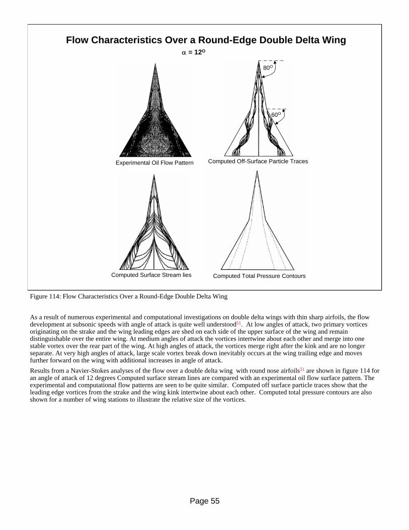
Figure 114: Flow Characteristics Over a Round-Edge Double Delta Wing
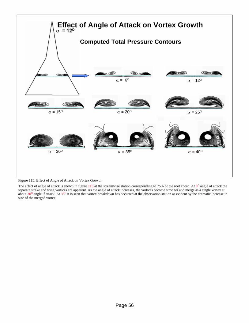
As a result of numerous experimental and computational investigations on double delta wings with thin sharp airfoils, the flow development at subsonic speeds with angle of attack is quite well understood51. At low angles of attack, two primary vortices originating on the strake and the wing leading edges are shed on each side of the upper surface of the wing and remain distinguishable over the entire wing. At medium angles of attack the vortices intertwine about each other and merge into one stable vortex over the rear part of the wing. At high angles of attack, the vortices merge right after the kink and are no longer separate. At very high angles of attack, large scale vortex break down inevitably occurs at the wing trailing edge and moves further forward on the wing with additional increases in angle of attack.Results from a Navier-Stokes analyses of the flow over a double delta wing with round nose airfoils51 are shown in figure 114 for an angle of attack of 12 degrees Computed surface stream lines are compared with an experimental oil flow surface pattern. The experimental and computational flow patterns are seen to be quite similar. Computed off surface particle traces show that the leading edge vortices from the strake and the wing kink intertwine about each other. Computed total pressure contours are also shown for a number of wing stations to illustrate the relative size of the vortices.
Page 56
Computed Total Pressure Contours
α = 6O
α = 20Oα = 15O
α = 12O
α = 30O
α = 25O
α = 40Oα = 35O
Effect of Angle of Attack on Vortex Growth
Figure 115: Effect of Angle of Attack on Vortex GrowthThe effect of angle of attack is shown in figure 115 at the streamwise station corresponding to 75% of the root chord. At 6O angle of attack the separate strake and wing vortices are apparent. As the angle of attack increases, the vortices become stronger and merge as a single vortex at about 30O angle if attack. At 35O it is seen that vortex breakdown has occurred at the observation station as evident by the dramatic increase in size of the merged vortex.

Page 57
0 10 20 30 40 50Angle of Attack deg.
1.4
1.2
1.0
0.8
0.6
0.4
0.2
0.0
Theory
Test
CL-2.0
-1.0
0.0
1.00 .25 .50 .75 1.0
Semi-Span Station η
CP
-2.0
-1.0
0.0
1.00 .25 .50 .75 1.0
Semi-Span Station η
CP
-2.0
-1.0
0.0
1.00 .25 .50 .75 1.0
Semi-Span Station η
CP
-2.0
-1.0
0.0
1.00 .25 .50 .75 1.0
Semi-Span Station η
CP
Pressure Distribution at X/CR = 0.75
α = 12O
α = 25O
α = 15O
α = 30OTheory
Test
Spanwise Pressure Distributions and Total Lift Coefficient• Navier-Stokes (Laminar)• Mach = 0.0• Rel = 1.3 x 10⁶
VortexBursting
Figure 116: Spanwise Pressure Distributions and Total Lift CoefficientCalculated pressure distributions for the double delta configuration are compared with experimental measurements in figure 116 for a number of angles of attack at the 75% root chord station. Up to 25O angle of attack, the computed pressure distributions are in approximate agreement with the test data although the theory under predicts the minimum pressure peaks induced by the vortices. There is a very large difference between the predicted and measured pressure distributions at 30O angle of attack. This apparently is due to the theory not predicting the severity of the vortex breakdown.The predicted and measured lift coefficients are also shown in figure 116. The theoretical lift curve is in excellent agreement with the test data up to slightly beyond 25O angle of attack in spite of the differences in the computed and measured pressure distributions. The test data data clearly shows that vortex bursting has occurred at about 26O angle of attack. The theory predicted vortex bursting to occur at about 30 degrees angle of attack The agreement between test and theory up to vortex bursting, seems to imply that the origin and overall strength of the vorticesare correctly predicted, despite the fact that the viscous dominated secondary vortex features are not adequately captured. .

Page 58
Wing/Body/Nacelles Flaps up
Wing/Body/Nacelles Outboard Flaps deflected δLE/δTE = 10O/3O
HSCT Wing Leading-Edge Pressure CharacteristicsMach = 0.90
Round Nose Airfoils
Sharp Nose Airfoils
Attached Flow
Attached Flow
UpperSurface
LE Vortex
UpperSurface
LE Vortex
LowerSurface
LE Vortex
LowerSurface
LE Vortex
Figure 117: HSCT Wing Leading-Edge Pressure Characteristics
An HSCT type configuration was tested in the National Transonic Facility, NTF, as part of the NASA’s High Speed Research Program. The primary objectives of the test programs2 were to assess the effects of Reynolds numbers on the aerodynamic characteristics of a realistic second generation supersonic transport at subsonic and transonic speeds, and to provide an experimental database for assessments of the advanced CFD computational methods.Achieving high Reynolds numbers in the NTF, requires variations of both total temperature and pressure. Consequently the wind tunnel model may encounter significant aeroelastic distortions. The effects of the aeroelastic distortions on the aerodynamic data are often of the same magnitude but opposite sense to that of the associated Reynolds number effects, thus masking the Reynolds numbers effects2. Thus it is important to establish the wind tunnel aeroelastic distortion and to adjust the wind tunnel data to a constant undistorted reference shape.Measured aerodynamic increments due to the aeroelastic distortions were used to adjust to adjust the wind tunnel data in Reference 2, to a constant dynamic pressure and thereby remove static aeroelastic effects from the analysis of Reynolds number effects.The HSCT model geometry shown in Figure 117, had round nose airfoils on the inboard portion of the wing planform. The airfoils on the reduced sweep outboard wing panel had sharp nose and rather thin airfoils. The wind tunnel data were obtained on the model for the supersonic cruise geometry without any flap deflections. and with outboard leading edge and trailing edge flap deflections to represented the transonic cruise geometry. Leading edge pressure measurements that were obtained close to the leading edge at one station on the inboard strake portion of the wing and one station on the outboard wing are also shown in figure 117 for a wide range of Reynolds number. As previously discussed on page 20 in conjunction with figure 79, the formation of the leading edge vortex at any station can be identified by the break in the CP versus angle of attack curve. Using this approach a range of angle of attack for attached flow can be identified at both the inboard and outboard stations shown in figure 117. The results once again indicate that the initial formation of the leading edge vortex is not dependent on Reynolds number. The pressures measured on the inboard portion of the wing vary with Reynolds number beyond the angle of attack for which the leading edge vortex first appears at that station. The pressures measured near the leading edge on the outboard portion of the wing which had thin sharp edge airfoils, are insensitive to the Reynolds number variations for the entire range of angle of attack.
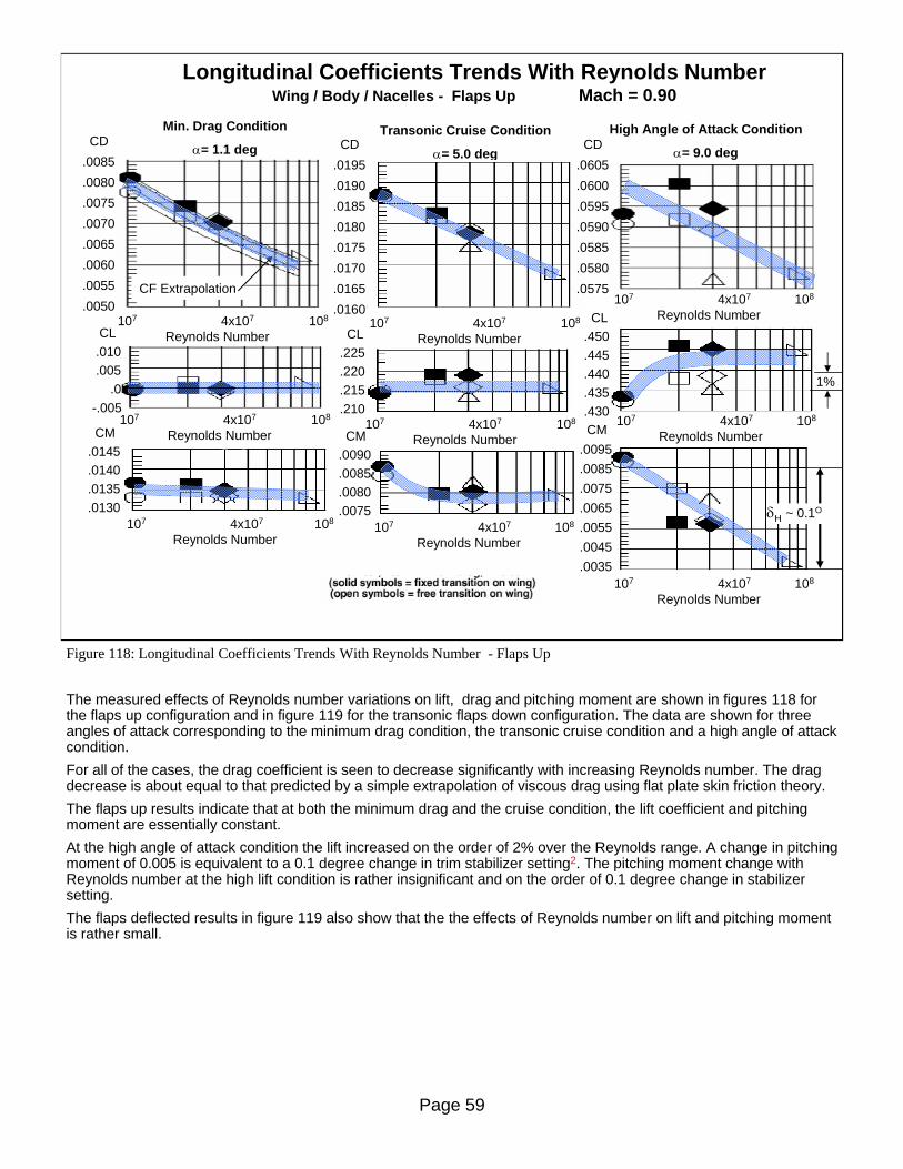
Page 59
107 4x10⁷ 108
Reynolds Number
CD.0085.0080.0075.0070.0065.0060.0055.0050
CM.0145.0140.0135.0130
107 4x10⁷ 108
Reynolds Number
Longitudinal Coefficients Trends With Reynolds NumberWing / Body / Nacelles - Flaps Up Mach = 0.90
Min. Drag Condition
α= 1.1 degTransonic Cruise Condition
α= 5.0 deg
CF Extrapolation
107 4x10⁷ 108
Reynolds Number
CM.0090.0085.0080.0075
CM.0095.0085.0075.0065.0055.0045.0035
107 4x10⁷ 108
Reynolds Number
107 4x10⁷ 108
Reynolds Number
CD.0195.0190.0185.0180.0175.0170.0165.0160
107 4x10⁷ 108
Reynolds Number
CD.0605.0600.0595.0590.0585.0580.0575
107 4x10⁷ 108
Reynolds Number
CL.010.005
.0-.005
107 4x10⁷ 108
Reynolds Number
CL.225.220.215.210
107 4x10⁷ 108
Reynolds Number
CL.450.445.440.435.430
High Angle of Attack Condition
α= 9.0 deg
1%
δH ~ 0.1O
Figure 118: Longitudinal Coefficients Trends With Reynolds Number - Flaps Up
The measured effects of Reynolds number variations on lift, drag and pitching moment are shown in figures 118 for the flaps up configuration and in figure 119 for the transonic flaps down configuration. The data are shown for three angles of attack corresponding to the minimum drag condition, the transonic cruise condition and a high angle of attack condition.For all of the cases, the drag coefficient is seen to decrease significantly with increasing Reynolds number. The drag decrease is about equal to that predicted by a simple extrapolation of viscous drag using flat plate skin friction theory.The flaps up results indicate that at both the minimum drag and the cruise condition, the lift coefficient and pitching moment are essentially constant. At the high angle of attack condition the lift increased on the order of 2% over the Reynolds range. A change in pitching moment of 0.005 is equivalent to a 0.1 degree change in trim stabilizer setting2. The pitching moment change with Reynolds number at the high lift condition is rather insignificant and on the order of 0.1 degree change in stabilizer setting.The flaps deflected results in figure 119 also show that the the effects of Reynolds number on lift and pitching moment is rather small.

Page 60
CM.0045.0040.0035.0030
107 4x10⁷ 108
Reynolds Number
Longitudinal Coefficients Trends With Reynolds NumberWing / Body / Nacelles - Flaps Deflected Mach = 0.90
Min. Drag Condition
α= 1.1 degTransonic Cruise Condition
α= 5.0 deg
CF Extrapolation
107 4x10⁷ 108
Reynolds Number
CM-.0005-.0010-.0015-.0020-.0025
CM-.0010-.0015-.0020-.0025-.0030-.0035-.0040
107 4x10⁷ 108
Reynolds Number
107 4x10⁷ 108
Reynolds Number
CD.0100.0095.0090.0085.0080.0075.0070.0065
107 4x10⁷ 108
Reynolds Number
CD.0180.0175.0170.0165.0160.0155.0150.0145
107 4x10⁷ 108
Reynolds Number
CD.0555.0550.0545.0540.0535.0530.0525
107 4x10⁷ 108
Reynolds Number
CL.025.020.015.010
107 4x10⁷ 108
Reynolds Number
CL.245.240.235.230
CL.470.465.460.455.450
High Angle of Attack Condition
α= 9.0 deg
107 4x10⁷ 108
Reynolds Number
1%
δH ~ 0.05O
Figure 119: Longitudinal Coefficients Trends With Reynolds Number - Flaps Deflected
Reference 1

Page 61
0 -1 -2CM
24
20
16
12
8
4
0
α degCL2.8
2.4
2.0
1.6
1.2
0.8
0.4
0.00 4 8 12 16 20 24
α deg
Attachment Line
Separation Line
Mach = 0.2α = 20O
β = 8O
ReC = 2 x 10⁶
0 4 8 12 16 20 24α deg
2.0
1.6
1.2
0.8
0.4
0.0
CL
⎝ ⎠
24
20
16
12
8
4
0
α deg
0 -2 -4 -6 -8CM
Attached FlowTheory
Attached FlowTheory
Attached FlowTheory
Attached FlowTheory
TestReD = 0.5 x 10⁶
TestReD = 0.5 x 10⁶
TestReD = 3.0 x 10⁶
ReD = 0.4 x 10⁶
TestReD = 3.0 x 10⁶
ReD = 0.4 x 10⁶
Mach = 1.6Circular Arc / Cylinder BodyRef Length = Body LengthRef Area = Base AreaMoment Center = Body Nose
Mach = 0.3Ogive / Cylinder BodyRef Length = Base DiameterRef Area = Base AreaMoment Center = Body Nose
Normal Force and Pitching Moment for Bodies of Revolution
Figure 120: Normal Force and Pitching Moment for Bodies of Revolution
VORTEX FLOW ON BODIES OF REVOLUTION AT ANGLE OF ATTACKExperimental studies as well as computational studies have shown that the flow around bodies of revolution at an angle of attackcan separate and form a pair of counter rotating vortices in much the same way as flow around a round nose airfoil can separate and form a leading edge vortex. Since the formation of the body vortices is predominately related to the body cross flow, the body vortices at both subsonic and supersonic conditions are quite similar. Results of experimental investigations of the normal force and pitching moment at angle of attack are shown in figure 120. The results show that at higher angles of attack a significant amount of vortex normal force can occur. The subsonic data shown in the figure indicates that the vortex lift generated by a body at angle of attack increases for larger Reynolds numbers.An HSCT configuration typically has a somewhat drooped nose that at the cruise condition is quite closely aligned with the free stream. Hence, little if any forebody lift would occur along the supersonic climb / cruise portion of the flight profile.

Page 62
Laminar FlowREC = 0.8 x 10⁶
Mach = 0.6α = 20O
Turbulent FlowREC = 0.8 x 10⁶
Mach = 0.6α = 20O
Turbulent FlowREC = 13.5 x 10⁶
Mach = 0.6α = 20O
Flight TestREC = 13.5 x 10⁶
Mach = 0.34α = 19O
F/A-18 Forebody Flow Characteristics at Angle of Attack of ~ 20O
Primary Separation
SecondarySeparation
Figure 121: F/A-18 Forebody Flow Characteristics at Angle of Attack of ~ 20O
Navier-Stokes analyses have been made of the forebody flow characteristics of the F/A-18 airplane at an angle of attack of 20 degrees55. The analyses were made for both laminar and turbulent flow. The turbulent analyses include two different Reynolds numbers. The lower Reynolds corresponds to wind tunnel test condition and the higher Reynolds number corresponded to a flight test condition.Computed total pressure contours and surface streamlines are shown in figure 121. The surface flow pattern obtained for the F/A-18 in flight is also shown in the figure.The laminar flow solution shows a primary separation line and a secondary separation line. The separations resulted in vary thinflat bubble type of separations. The turbulent flow patterns are significantly different then the laminar results. The primary and secondary forebody separations were totally eliminated by the turbulent flow.The forebody flow patterns for the turbulent analyses cases are not affected by the Reynolds numbers differences. The calculatedturbulent flow pattern closely matches the flight test flow pattern.

Page 63
A
C
B
A
B C
θ = 0O Bottom of Body Noseθ = 180O Top of Body Nose
Comparison of Predicted and Measured Forebody PressuresMach = 0.6 ReC = 0.8 x 10⁶ α = 20 deg.
Figure 122: Comparison of Predicted and Measured Forebody PressuresWind tunnel pressure measurements obtained around the forebody at three stations, are compared with the corresponding theoretical predictions in figure 122. The turbulent predictions closely match the test data except at the first station where the theory slightly under predicts the test results around the upper part of the forebody. In spite of the significant differences in the laminar and turbulent surface flow patterns, the calculated fore body pressure distributions were nearly identical.

Page 64
CFL3D ViscousAnalysis
CFL3D InviscidAnalysis
Forebody Chine AnalysesM∞ = 0.4Re = 2.4 x 10⁶ per footα = 19.8O
Figure 123: Forebody Chine AnalysesA coordinated CFD study and wind tunnel program was conducted to evaluate the ability of the CFD to capture the details of the complex flow development on a forebody chine configurationxx. The theoretical methods included both Euler and Navier-Stokes turbulent flow analyses. The sharp edges of the chine act much like a sharp edge airfoil in initiating a leading edge vortex. Results from that activity are shown in figures 123 through 125.Total pressure contours obtained by the Euler and Navier-Stokes are shown in the composite image in Figure 123. The Euler solution shows the formation and growth of the primary vortex that was obviously initiated by the numerical viscosity in the solution process. The viscous results show the formation of the primary vortex, the induced secondary vortex and the boundary layer growth along the body. Relative to the viscous solution, the inviscid primary core appears to be more compact then the viscous primary core.

Page 65
M∞ = 0.4Re = 2.4 x 10⁶ per footα = 19.8O
Comparison of Predicted and Experimental Forebody PressuresStarboard
DataPortViscous ( Baldwin-Lomax)
CFL3DInviscid
USM3D Inviscid
Figure 124: Comparison of Predicted and Experimental Forebody PressuresExperimental spanwise pressure measurements are compared with the viscous and inviscid solutions in figure 124. The Navier-Stokes predictions agree very well with the test data at the second and the third station. This suggests that the secondary vortex effects are correctly captured in the theoretical analyses. The agreement at the first station was not as good as for the aft two stations. The results however clearly show the viscous effects on the pressure distributions.
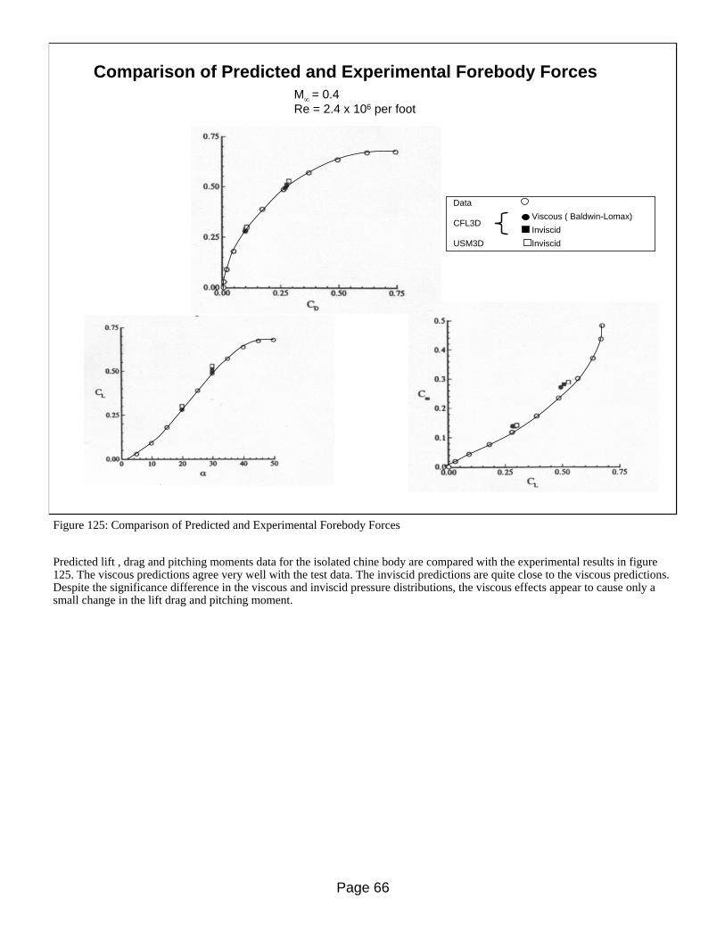
Page 66
Comparison of Predicted and Experimental Forebody Forces
DataViscous ( Baldwin-Lomax)
CFL3DInviscid
USM3D Inviscid
M∞ = 0.4Re = 2.4 x 10⁶ per foot
Figure 125: Comparison of Predicted and Experimental Forebody Forces
Predicted lift , drag and pitching moments data for the isolated chine body are compared with the experimental results in figure 125. The viscous predictions agree very well with the test data. The inviscid predictions are quite close to the viscous predictions. Despite the significance difference in the viscous and inviscid pressure distributions, the viscous effects appear to cause only a small change in the lift drag and pitching moment.
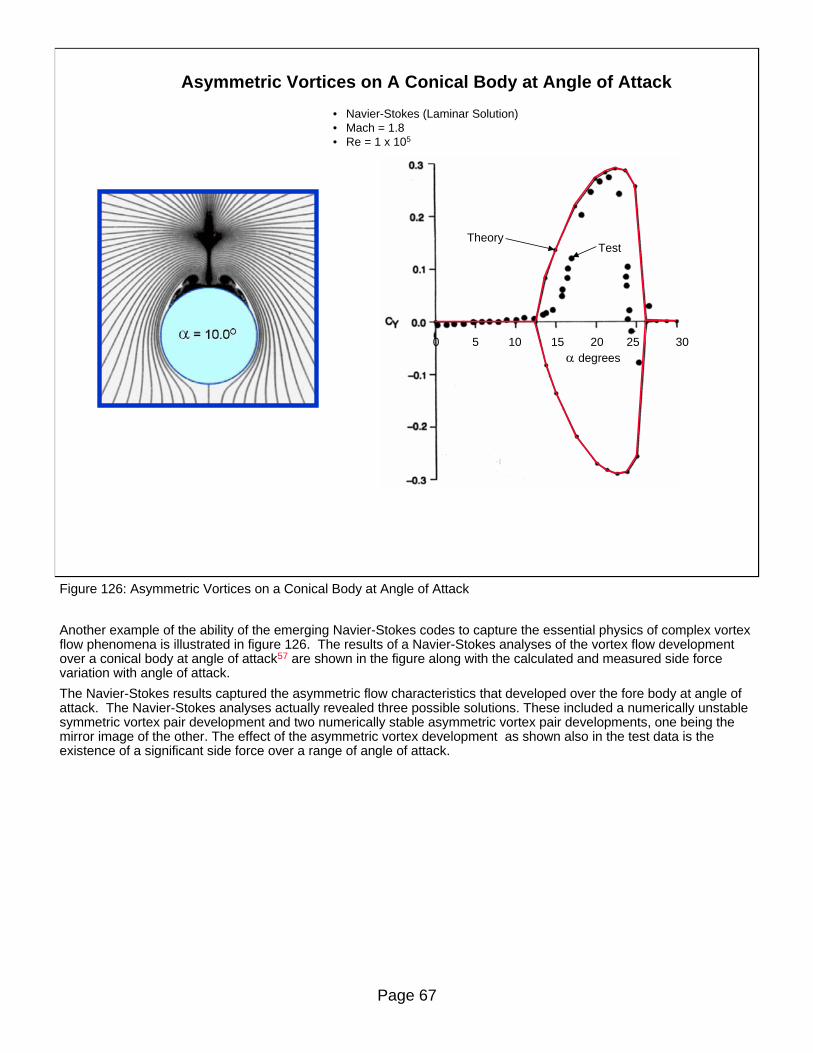
Page 67
Asymmetric Vortices on A Conical Body at Angle of Attack
0 5 10 15 20 25 30α degrees
• Navier-Stokes (Laminar Solution)• Mach = 1.8• Re = 1 x 10⁵
TestTheory
Figure 126: Asymmetric Vortices on a Conical Body at Angle of Attack
Another example of the ability of the emerging Navier-Stokes codes to capture the essential physics of complex vortex flow phenomena is illustrated in figure 126. The results of a Navier-Stokes analyses of the vortex flow development over a conical body at angle of attack57 are shown in the figure along with the calculated and measured side force variation with angle of attack.The Navier-Stokes results captured the asymmetric flow characteristics that developed over the fore body at angle of attack. The Navier-Stokes analyses actually revealed three possible solutions. These included a numerically unstable symmetric vortex pair development and two numerically stable asymmetric vortex pair developments, one being the mirror image of the other. The effect of the asymmetric vortex development as shown also in the test data is the existence of a significant side force over a range of angle of attack.
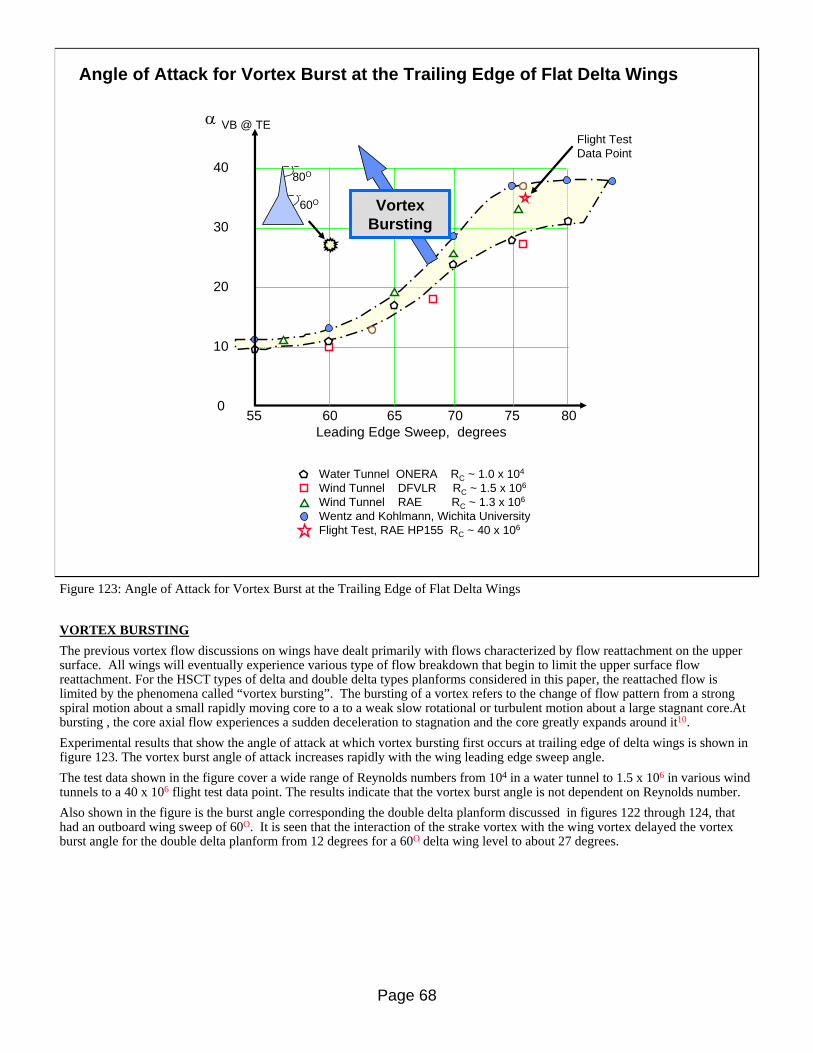
Page 68
Angle of Attack for Vortex Burst at the Trailing Edge of Flat Delta Wings
Water Tunnel ONERA RC ~ 1.0 x 10⁴
Wind Tunnel DFVLR RC ~ 1.5 x 10⁶
Wind Tunnel RAE RC ~ 1.3 x 10⁶
Wentz and Kohlmann, Wichita UniversityFlight Test, RAE HP155 RC ~ 40 x 106
55 60 65 70 75 80Leading Edge Sweep, degrees
40
30
20
10
0
α VB @ TE
Vortex Bursting
80O
60O
Flight Test Data Point
Figure 123: Angle of Attack for Vortex Burst at the Trailing Edge of Flat Delta Wings
VORTEX BURSTINGThe previous vortex flow discussions on wings have dealt primarily with flows characterized by flow reattachment on the upper surface. All wings will eventually experience various type of flow breakdown that begin to limit the upper surface flow reattachment. For the HSCT types of delta and double delta types planforms considered in this paper, the reattached flow is limited by the phenomena called “vortex bursting”. The bursting of a vortex refers to the change of flow pattern from a strong spiral motion about a small rapidly moving core to a to a weak slow rotational or turbulent motion about a large stagnant core.At bursting , the core axial flow experiences a sudden deceleration to stagnation and the core greatly expands around it10.Experimental results that show the angle of attack at which vortex bursting first occurs at trailing edge of delta wings is shown in figure 123. The vortex burst angle of attack increases rapidly with the wing leading edge sweep angle. The test data shown in the figure cover a wide range of Reynolds numbers from 104 in a water tunnel to 1.5 x 10⁶ in various wind tunnels to a 40 x 106 flight test data point. The results indicate that the vortex burst angle is not dependent on Reynolds number.Also shown in the figure is the burst angle corresponding the double delta planform discussed in figures 122 through 124, that had an outboard wing sweep of 60O. It is seen that the interaction of the strake vortex with the wing vortex delayed the vortex burst angle for the double delta planform from 12 degrees for a 60O delta wing level to about 27 degrees.

Page 69
0 .1 .2 .3 .4 .5 .6 .7 .8 .9 1.0X/L
50
45
40
35
30
25
20
15
10
5
0
α, deg
Flight, smoke, M∞ =0.3, RC = 10x106
Flight, natural condensation, M∞ =0.3, RC = 10x106
Wind tunnel, vapor screen, M∞ =0.4, RC = 2x10⁶
Wind tunnel, smoke, M∞ =0.1, RC = 1x10⁶
Navier Stokes predictions, M∞ =0.3, RC = 10x106
Reynolds Number Effects on LEX Primary Vortex Breakdown LocationCorrelations Between Flight, Wind Tunnel and Computational Results
Theory
Wind TunnelAnd Flight test
Figure124: Reynolds Number Effects on LEX Primary Vortex Breakdown Location
Figure 124 shows predicted LEX primary vortex breakdown locations along with those observed in various wind tunnel experiments and also from a number of different flight tests for the F/A-184. The results show the rate of forward movement of the vortex breakdown location with increasing angle of attack. These results also indicate that vortex bursting is not Reynolds number dependent.The theoretical predictions again predict a higher burst angle of attack then indicated by the experimental data. This is consistent with the results shown in figure 116. The theory does appear to predict the rate of forward movement of the vortex burst location with angle of attack correctly.

Page 70
• Wing Planform Airfoils Nose Have a Significant Effect on the Origin and Growth of the L.E. Vortex
• Reynolds Number Has Little Effect on the Vortex Development on a Wing With Sharp / ThinAirfoils.
• Leading Edge Vortex Growth on a Wing With Round Nose Airfoils Does Not Appear to be Dependent on Reynolds Number for Turbulent Flow.
• Pressure Distributions With Vortex Flow on Wings With Rounded Edges appear not overly sensitiveto Reynolds Numbers Variations.
• Euler Predictions of the Forces on Wings With Sharp Edges Appear to Match the Test Data Even Though the Pressure Distributions May Differ Significantly in the Region of the Secondary Vortices.
• Navier-Stokes Predictions Capture the Details of the Leading Edge Vortex on Both Round Nose and Sharp Nose Airfoils Including the Primary and the Secondary Vortices.
• Predicted Surface Pressures in the Region of the Secondary Vortices Typically do Not Closely matchthe Test Data, but the Resulting Total Forces and Moments do Match the Test Data.
• Vortices Shed by the Forebody at Angle of Attack Appear Sensitive on the Nature of the Boundary layer ( ie Laminar or Turbulent)
• The CFD Codes Offer Great Promise in Prediction the Forebody Vortices. Additional Systematic Test Versus Theory Studies Should be Conducted to Fully Establish the Validity of the CFD Predictions.
• Vortex Bursting Does Not Appear to be Reynolds Number Dependent.
• The CFD Codes Appear to Predict Higher Angles of Attack for Vortex Bursting Then the Test Data.
Conclusions: Leading Edge Vortex Flows

Page 71
References1. Owens, L.R., Wahls, R.A., “Reynolds Number Effects on a Supersonic Transport at Subsonic High-Lift Conditions”, AIAA-
2001-0911, Jan. 20012. Wahls, R.A., Owens, L.R. and Rivers, S.M.B. Rivers, “ Reynolds Number Effect on a Supersonic Transport at Transonic
Conditions”, AIAA-2001-0912, Jan 20013. Owens, L.R., Wahls, R.A., Elzey, M.B., and Hamner, M.P., “Reynolds Number Effects on the Stability & Control
Characteristics of a Supersonic Transport”, AIAA-2002-0417, Jan 20024. Fisher, D.F., et al, “Reynolds Number Effects at High Angles of Attack”, AIAA-98-2879, June 19985. Tomek, W.G., Hall, R.M., Wahls, R.A., Luckring, J.M., and Owens, L.R., “Investigation of Reynolds Effects on a Generic
Fighter Configuration in the National Transonic Facility”, AIAA-2002-0418, Jan. 20026. Niewald, P.W., and Parker, S.L., “Wind-Tunnel Techniques to Successfully Predict F/A-18E In-Flight Lift and Drag”, Journal
Of Aircraft, Vol. 37, No. 1, Jan-Feb 2000, pp 9-147. Niewald, P.W., and S.L. Parker, ”Flight-Test Techniques Employed To Successfully Verify F/A-18E In-Flight Lift and
Drag”, Journal of Aircraft Vol. 37, No 2, Mar – Apr 2000, pp 194-2008. Kulfan, R.M., Sigalla, A., “Real Flow Limitations in Supersonic Airplane Design:, AIAA-78-147, Jan. 19789. Kulfan, R.M., Sigalla, A., “Real Flow Limitations in Supersonic Airplane Design:, Journal of Aircraft, Vol. 16 No. 10, pp
645-658, Oct. 197910. Kulfan, R. M., “Wing Airfoil Effects on the Development of Leading Edge Vortices”, AIAA-79-1675, Aug 197911. Kulfan, R.M., “Wing Geometry Effects on Leading Edge Vortices”, AIAA-79-1872, Aug 197912. Ornberg, T., “A Note on the Flow Around Delta Wings”, KTH-Aero TN38, Feb 195413. Kuchemann, D., “Types of Flows on Swept Wings”, Journal of the Royal Aeronautical Society, vol. 57, pp 683-699, Nov
1953, 14. Stanbrook,A., and Squire, L.C., “Possible Types of Flow at Swept Leading Edges”, The Aeronautical Quarterly, Feb 1964, pp
72-8215. Polhamus, E.C., “A Concept of the Vortex Lift of Sharp-Edged Delta Wings Based on a Leading Edge Suction Analogy”,
NASA TND-3767, 196616. Polhamus, E.C., “Predictions of Vortex-Lift Characteristics by a Leading-Edge-Suction-Analogy”, Journal of Aircraft, Vol.8,
No. 4, April 197117. Miller,D.S., Wood, R.M., and Covell, P.F., “An Overview of the Fundamental Aerodynamics Branch’s Research Activities in
Wing Leading-Edge Vortex Flows at Supersonic Speeds”, NASA Conference Publication 2416, Vortex Flow Aerodynamics, Vol 1 pp 349-378, Oct 1985
18. Hollenback, D.M., and Blom, G.A., Applications of a parabolized Navier-Stokes Code to an HSCT Configuration and Comparison to Wind Tunnel Data”, AIAA-93-3537, August 1993
19. Blom, G.A., Ball, D.N., Bussoletti, J.E., and Yu, N.J., “Computations of the Supersonic Flow Over an HSCT Type Configuration and Comparison With Wind Tunnel Data”, AIAA-91-3290, Sept. 1991 Nelson, C.P., “Effects of Wing Planform on HSCT Off-Design Aerodynamics”, AIAA-92-2629, June 1992
20. Cliff, S.E., Reuther, J.J., Saunders, D.A., and Hicks, R.M., “Single-Point and Multipoint Aerodynamic Shape Optimization of High-Speed Civil Aircraft”, Lournal of Aircraft, Vol. 38, No.6, Nov.-Dec., 2001, pp 997-1005
21. Kim, H-J., Shigeru, O., and Nakahashi, K., “Flap-Deflection Optimization for Transonic Cruise Performance Improvement of Supersonic Transport Wing”, Journal of Aircraft, Vol. 38, No. 4, Jul.-Aug,. 2001, pp 709-717
22. Rivers, M. B. and Wahls, R. A., “Turbulence Model Comparisons for a High-Speed Aircraft”, NASA CDTP-1012, November 1997, NASA/TP-1999-209540, Dec. 1, 1999, LaRC 1.
23. Kulfan, R. M.., “Historic Background on Flat Plate Turbulent Flow Skin Friction and Boundary Layer Growth.”, 1998 NASA High-Speed Research Program Aerodynamic Performance Workshop, Vol. 1, Part 1 Page: 477-513, Dec 01, 1999, NASA/CP-1999-209692/Vol. 1/Pt. 1
24. Kulfan, B.M., “Assessment of CFD Predictions of Viscous Drag” AIAA-2000-2391, June 2000 1.25. Bardina, J. E., Huang, P. G. and Coakley, T. J., “Turbulence Modeling Validation, Testing, and Development”, NASA TM-
110446, April 1977 26. Baldwin, B. and Lomax, H., “Thin-Layer Approximation and Algebraic Model for Separated Turbulent Flows”, AIAA-78-
257, January 1978 27. Degani, D., Schiff, L. B.and Levy, Y., “Physical Considerations Governing Computation of Turbulent Flows”, AIAA-90-
0096, January 1990
Page 72
28. Spalart, P. R. and Allmaras, S. R., “A One-Equation Turbulence Model for Aerodynamic Flows”, AIAA-92-0439, January 1992 29. Menter, F. R., “Assessment of Two-Equation Turbulence Models for Transonic Flows”, AIAA 94-2343, June 1994 30. Menter, F. R., “Two-Equation Eddy-Viscosity Turbulence Models for Engineering Applications:, AIAA Journal, vol. 32, no. 8, August 1994, pp.
357-37231. Carlson, J.R., “Prediction of Very High Reynolds Number Compressible Skin Friction”, AIAA-98-2880, 198832. Thibert, J.J., “The Aerodynamics of the Future Supersonic Transport Aircraft: Research Activities at ONERA”, Paper No 18 in Fluid Dynamics
Research on Supersonic Aircraft, RTO EN-4, May 1998 33. Fisher, D.F., “Boundary Layer, Skin Friction, and Boattail Pressure Measurements From the YF-12 Airplane at Mach Numbers up to 3”, NACA
CP-2054, Volume 1, Sept. 197834. Czarnecki, K.R., “The Problem of Roughness Drag at Supersonic Speeds”, NASA SP-124, Conference on Aircraft Aerodynamics, May 196635. Goldstein, S., MODERN DEVELOPMENTS IN FLUID DYNAMICS,Dover publications 1965 36. Chang, P.K., SEPARATION OF FLOW, Pergamon Press, 197037. Panaras, A.G., “Review of the Physics of Swept-Shock / Boundary Layer Interactions”, Prog. Aerospace Sci. vol 31, pp 173-244, 199538. Cliff, S.E, et al, “Simulated Inlet Unstart and Nacelle /Diverter Effects for the Boeing Reference H Configuration”, Feb 199639. Polhamus, E.C., Vortex Lift Research : Early Contributions and Some Current Challenges”, NASA Conference Publication 2416, Vortex Flow
Aerodynamics, Vol 1 pp 1-30, Oct 198540. Leading-Edge Vortex Research: “Some Non-planar Concepts and Current Challenges”, NASA Conference Publication 2416, Vortex Flow
Aerodynamics, Vol 1 pp 31-64, Oct 198541. Poisson-Quinton, Philippe, “Slender Wings for Civil and Military Aircraft” 8th Theodore Von Karman Memorial Lecture, Twentieth Israel Annual
Conference on Aviation and Astronautics, Feb. 197842. Lamar, J.E., “In-Flight and Wind Tunnel Leading Edge Vortex Study on the F-106B Airplane”, NASA Conference Publication 2416, Vortex
Flow Aerodynamics, Vol 1 pp 187-202, Oct 198543. Manro, M.E., Manning,K., Hallstaff, T.H., and Rogers, J.Y., “ Transonic Pressure Measurements and Comparison of Theory to Experiment for
an Arrow Wing Configuration”, NASA CR-2610, NASA CR-132727, NASA CR-132728, NASA CR-132729, August 1976.44. Manro, M.E., Tinoco, E.N., Bobbit, P.H., and Rogers, J.T., “Comparison of Theoretical and Experimental Pressure distributions on an Arrow
Wing Configuration at Transonic Speeds”, AERODYNAMIC ANALYSIS REQUIRING ADVANCED COMPUTERS, NASA SP-347, PP 1141-1188, 1975
45. Chu, J.C., and Luckring, J.M., “Experimental Surface Pressure Data Obtained on a 65O Delta Wing Across Reynolds Number and Mach Number Ranges:, NASA Technical Memorandum 4645, Volumes 1, 2 and 3 and Supplements to Volumes 1, 2 and 3, Feb 1996
46. Rizzi, A., Muller, B., “Comparison of Euler and Navier Stokes Solutions for Vortex Flow Over a Delta Wing”, Aeronautical Journal, pp 145-153, April 1988
47. Muller, B., and Rizzi, A., “Navier-Stokes Computation of Transonic Vortices over a round Leading Edge Delta wing”, AIAA-87-1227, June 198748. Londenberg, W.K., “Transonic Navier-Stokes Calculations About a 65O Delta Wing”, NASA Contractor Report 4635, Nov. 199449. McMillin, S.N., Pittman, J.L., and Thomas, J.L., “Computational Study of Incipient Leading Edge Separation on a Supersonic Delta Wing”,
Journal of Aircraft Vol 29, No. 2, Mar – April 199250. Webster, W.P., and Shang, J.S., “Thin-Layer Full Navier-Stokes Simulations over a supersonic Delta Wing”, AIAA Journal Vol. 29, No. 9,
September 1991, pp 1363 to 136951. Liu, M.J., et al, :Flow Patterns and Aerodynamic Characteristics of a Wing – Strake Configuration”, Journal of Aircraft, Vol. 17, No. 5, pp 332 –
337, May 198052. Hsu, C.H., and Liu, C.H., “Navier-Stokes Computations of Flow around a Round-Edged Double-Delta Wing”, AIAA Journal Vol. 28, NO. 6,
June 1990, pp 961-96853. Nelson, C.P., “Effects of Wing Planform on HSCT Off-Desigm Aerodynamics”, AIAA-92-2629, June 199254. Ghaffari, F., “On the Vortical-Flow Prediction Capability of an Unstructured-Grid Euler Solution”, AIAA-94-0163, Jan. 199455. Siclari, M.J., and Marconi, F., “Computation of Navier-Stokes Solutions Exhibiting Asymmetric Vortices”, Aiaa Journal Vol. 29, NO. 1, pp32-4256. Lan, C.E., “ Extensions of the Concept of Suction Analogy to Prediction of Vortex Lift Effect.”, NASA CP 2416, VORTEX FLOW
AERODYNAMICS, Oct 1985, pp 65-8457. Gharrari, F., Luckring, J.M., and Thomas, J.L., “Navier-Stokes Solutions About the F/A-18 Forebody-Leading-Edge Extension Configuration”,
Journal of Aircraft, Vol. 27, NO. 9, Sept 1990, pp 737-748

Page 73
Versions of Charts For Paper

Page 74
α = 12O
Experimental Oil Flow Pattern
Computed Surface Stream lies
Computed Off-Surface Particle Traces
Computed Total Pressure Contours
Flow Characteristics Over a Round-Edge Double Delta Wing
80O
40O
Figure 109 114: Flow Characteristics Over a Round-Edge Double Delta WingThe current concepts for HSCT type configuration typically incorporate a double delta wing planform. These planforms have a highly swept inboard wing panel with round nose airfoils and a reduced sweep outer wing panel with sharp thin airfoils to provide a balance between the desire for slender wing geometry for supersonic cruise performance and increased span for low speed high lift performance.The flow over these wings at the design condition is well behaved attached flow. At off design conditions leading edge vortices may develop on the strake. The strake vortex flowing aft can have a significant effect on the outer wing panel. The flow at supersonic conditions is not too dissimilar then that at subsonic conditions. Some insight can be gained by examining results obtained initially obtained at subsonic speeds.

Page 75
Asymmetric Vortices on A Conical Body at Angle of Attack
0 5 10 15 20 25 30α degrees
• Navier-Stokes (Laminar Solution)• Mach = 1.8• Re = 1 x 10⁵
TestTheory
10O
12.5O
26.3O13.8O
25O20O
15O
21.3O
22.5O
17.5O 23.8O
27.5O