rice university on-orbit transfer trajectory methods … · · 2017-12-15on-orbit transfer...

RICE UNIVERSITY

On-Orbit Transfer Trajectory Methods

Using High Fidelity Dynamic Models

by

Danielle Burke

A THESIS SUBMITTED

IN PARTIAL FULFILLMENT OF THE

REQUIREMENTS FOR THE DEGREE

Master of Science

APPROVED, THESIS COMMITTEE:

i i i i V'' 1 ; \ • v

Pol Spanos L.B. Ryon Chair of Engineering

Andrew Dick Ls Mechanical Engineering & Materials Science

Andrew Meade Mechanical Engineering & Materials Science

faz Bedrossian C.S. Draper Laboratory

Ellis King C.S. Draper La^OKtfory

HOUSTON, TEXAS

APRIL, 2010

UMI Number: 1486020

All rights reserved

INFORMATION TO ALL USERS The quality of this reproduction is dependent upon the quality of the copy submitted.

In the unlikely event that the author did not send a complete manuscript and there are missing pages, these will be noted. Also, if material had to be removed,

a note will indicate the deletion.

UMT Dissertation Publishing

UMI 1486020 Copyright 2010 by ProQuest LLC.

All rights reserved. This edition of the work is protected against unauthorized copying under Title 17, United States Code.

ProQuest LLC 789 East Eisenhower Parkway

P.O. Box 1346 Ann Arbor, Ml 48106-1346

1

The views expressed in this thesis are those of the author and do not reflect the

official policy or position of the United States Air Force, Department of Defense, or

the U.S. Government.

u

Abstract

On-Orbit Transfer Trajectory Generation Methods Using High Fidelity Dynamic

Models

by

Danielle Burke

A high fidelity trajectory propagator for use in targeting and reference trajectory

generation is developed for aerospace applications in low Earth and translunar orbits.

The dominant perturbing effects necessary to accurately model vehicle motion in

these dynamic environments are incorporated into a numerical predictor-corrector

scheme to converge on a realistic trajectory incorporating multi-body gravitation,

high order gravity, atmospheric drag, and solar radiation pressure. The predictor-

corrector algorithm is shown to reliably produce accurate required velocities to meet

constraints on the final position for the dominant perturbation effects modeled. Low

fidelity conic state propagation techniques such as Lambert's method and multiconic

pseudostate theory are developed to provide a suitable initial guess. Feasibility of

the method is demonstrated through sensitivity analysis to the initial guess for a

bounding set of cases.

iii

Acknowledgments

The journey to completion of this thesis has been a long and arduous process that

could not have been made possible without the help of a number of individuals. I

would like to thank my Rice University advisor, Professor Pol Spanos, for supporting

my research and coursework at Rice. I additionally would like to thank Nazareth

Bedrossian of the C.S. Draper Laboratory who gave me the opportunity to come to

Houston and work on this research. I would like to thank my advisor at Draper, Ellis

King, for all of his guidance and support. Special thanks to my thesis committee,

Pol Spanos, Andrew Dick, Andrew Meade, Nazareth Bedrossian, and Ellis King for

valuable input and feedback on this research. Furthermore, Stan Sheppherd for tak

ing the time to review my thesis and provide insightful inputs. Additionally, Zoran

Milenkovic who was there to help when it seemed that the obstacles were insurmount

able. Thanks to my colleagues with whom I shared an office for two years, they made

this journey an unforgettable adventure: John who kept the room entertained with

his ridiculous music, Eric who will forever be the MATLAB Graph Master, and Adam

who will one day eat Chinese food and enjoy it. I would like to thank my husband

who pushed me to see the final goal, never accepting my complaints. Finally, thanks

to my mom who realized that not talking about the thesis was sometimes the best

advice of all.

Contents

Abstract ii

Acknowledgements iii

List of Figures xvi

List of Tables xviii

1 Introduction 1

2 Special Perturbation Techniques 6

2.1 Orbital Elements 6

2.2 Two-body Equations of Motion 9

2.3 Kepler's Equation 11

2.4 Equations of Motion with Perturbations 15

2.5 CowelPs Method 17

2.6 Encke's Method 19

2.6.1 Rectification 21

2.7 Variation of Parameters 23

2.8 Numerical Integration Methods 24

2.8.1 Integration Errors 24

2.8.2 Euler's Method 27

iv

V

2.8.3 Runge-Kutta Method 28

2.8.4 Nystrom Integration Method 31

2.8.5 MATLAB Solvers 32

3 Development of Propagator 37

3.1 System Overview 37

3.2 Three Body Motion 38

3.2.1 SPICE 39

3.3 High Order Gravity 42

3.3.1 Formulation 43

3.3.2 High Order Gravity Moon 50

3.3.3 Validation of Higher Order Gravity Model 51

3.3.4 Model Configuration 59

3.4 Atmospheric Drag 60

3.5 Solar Radiation 63

4 State Transition Matrix 68

4.1 N-Body Partials 71

4.2 Gravity Potential Partials 73

4.3 Atmospheric Drag Partials 77

4.4 Accuracy of Error State Transition Matrix 79

4.4.1 Low Earth Orbit Transfer Test Results 82

4.4.2 Translunar Transfer Test Results 85

4.5 Shooting Method 90

5 Translunar Application 93

5.1 Pseudostate Theory for Approximating Three-Body Trajectories . . . 94

5.1.1 Conic Approximations 95

5.1.2 Overlapped Conic Approximation 100

vi

5.1.3 Pseudostate Theory 105

5.1.4 Translunar Targeting 107

5.2 EXLX Configuration I l l

5.2.1 Parameter Selection User Interface I l l

5.2.2 EXLX Multi-Conic Propagator 114

5.3 Test Case Selection 116

5.4 Results and Analysis 121

5.4.1 Translunar Shooting Method Sensitivity 124

5.5 Conclusion 135

5.5.1 Method Limitations 135

5.5.2 Summary of Test Results 136

6 Low Earth Orbit Application 138

6.1 Lambert's Method 138

6.1.1 Lagrange's Equations 139

6.1.2 Gauss's Formulation 142

6.1.3 Battin's Combined Equation 144

6.2 Test Case Selection 146

6.3 Results and Analysis 150

6.4 Conclusions 162

6.4.1 Method Limitations 162

6.4.2 Summary of Test Results . . . . . . . . . . . . . . . . . . . . . 167

7 Closure 170

A Feasible Translunar Trajectories 177

B Monte Carlo Sample Size 182

C List of Test Cases 184

Vll

D LEO Contour Maps 188

List of Figures

1.1 Illustration of a generalized Hohmann transfer between two low Earth

orbits 2

1.2 Illustration of a generalized translunar transfer 4

2.1 Illustration of the classic orbital elements: inclination (i), right ascen

sion of ascending node (fi), argument of perigee (a;), and true anomaly

iy) [49] 7

2.2 Elliptical orbit conic section illustrating the two foci, F and F', as well

as the semimajor axis, (a) [49] 8

2.3 Geometry of Kepler's equation [49] 12

2.4 A representation of a spherical coordinate system [53] 18

2.5 Vector definition for Encke's method [43] 20

2.6 Boxplot comparison of the magnitude difference in final position of

Cowell/Encke propagation and Kepler's analytical solution for 7,000

low Earth orbits over one orbit period 23

2.7 Comparison of Euler's Method, second-order Runge Kutta method,

and fourth-order Runge-Kutta method where the black dots represent

the estimated values and the red dots are the intermediate points . . 30

2.8 Comparison of computation time between MATLAB's ODE solvers . 34

2.9 Comparison of required number of steps between MATLAB ODE solvers 35

viii

IX

2.10 Comparison of magnitude difference in final position between the in

tegrated value and Kepler's analytical solution for MATLAB's ODE

solvers 36

3.1 Configuration of the Cowell propagator 38

3.2 Illustration of the Earth's zonal harmonics with shaded regions repre

senting additional mass [49] 43

3.3 Illustration of the Earth's tesseral harmonics with shaded regions rep

resenting additional mass [49] 43

3.4 Three body configuration of position vectors between the Earth, Moon,

and satellite 51

3.5 Radial component of the gravitational perturbation, aj3_9 (^) , due

to higher order gravity up to degree 9 excluding J2 with respect to

latitude/longitude 53

3.6 Earth's gravity field anomalies (mGal) as determined by GRACE [2] . 54

3.7 The gravitational pull of the Earth's equatorial bulge causes the orbital

plane of an eastbound satellite to regress westward 55

3.8 Deviation in final position (km) due to J2-9 for circular orbits with

varying altitudes and inclinations propagated over one period 56

3.9 Deviation in final position (km) due to J3_9 for circular orbits with

varying inclinations and ascending nodes at a = 100 km propagated

over one period 57

3.10 Deviation in final position (km) due to J^s for circular orbits with

varying ascending nodes and inclinations at a = 100 km propagated

over one period 58

3.11 General illustration of the Earth's atmosphere with the bands repre

senting areas of similar properties [49] 62

X

3.12 Geometry used by the program Shadow to calculate the regions of

penumbra and umbra experienced by the vehicle [49] 65

4.1 Illustration of 180° low Earth orbit transfer between two orbits with

i = 0° and e = 0.1 83

4.2 Individual perturbation magnitudes for 180° low Earth orbit transfer

between two orbits with i = 0° and e = 0.1 84

4.3 Magnitude difference in predicted position error between Cowell and

the state transition matrix for a LEO transfer over varying transfer times 85


the state transition matrix for a LEO transfer over varying initial per

turbation percentages 86

4.5 Illustration of a 5 day translunar transfer with conditions i e = 16°

ftffi = 71° and iQ = 15° ft© = 100° 87

4.6 Individual perturbation magnitudes for translunar transfer between a

low Earth orbit with i — 16° ft = 71° and a low lunar orbit with i = 15°

ft = 100° 88


the state transition matrix for a translunar transfer over varying times 89


the state transition matrix for a translunar transfer over varying initial

perturbation percentages 89

4.9 Illustration of Lambert shooting method . . . . . . . . . . . . . . . . 91

4.10 Flow chart summary of the higher order Lambert method formulation 92

5.1 General illustration of translunar transfer between TLI and LOI . . . 94

5.2 Summary of translunar transfer velocity computation and shooting

method application 95

xi

5.3 Definition of interior and exterior points for overlapped conic approxi

mation 101

5.4 Pseudostate terminals for a short segment of a transhmar trajectory . 108

5.5 Pseudostate terminals for a circumlunar segment of a translunar tra

jectory 109

5.6 Pseudostate terminal geometry for translunar targeting problem . . . 110

5.7 Example of EXLX Excel lunar parking orbit accessibility scan matrix 113

5.8 Example of EXLX Excel timetable scan matrix 114

5.9 Perturbation dynamics applied in each flight phase for the EXLX and

Cowell propagators over a translunar trajectory 115

5.10 Tilt of the Earth and Moon with respect to the ecliptic plane 116

5.11 Contour plot of lunar orbit insertion AV for an initial Earth orbit with

i@ = 0° and Q e = 0°. The white lines represent lunar orbit parameter

regions that meet the constraint of AVmax = 840 km/s 118

5.12 Contour plot of feasible lunar orbit parameters for varying initial Earth

orbit parameters 119

5.13 Distribution of Earth and lunar orbital elements for 110 test cases . . 121

5.14 Histogram of the iteration number for the 110 translunar test cases . 122

5.15 Convergence rate for a range of translunar cases with iteration numbers

within 1.5IQR as well as the rate for the three outlier cases 123

5.16 Translunar trajectories at LOU for a variety of test cases 123

5.17 Example of a translunar transfer into a lunar prograde orbit (Test Case

#77) 124

5.18 Example of a translunar transfer into a lunar retrograde orbit (Test

Case #71) 125

5.19 Histogram of the change in |AV| required for the translunar test cases 125

5.20 Stem plot of |AV| based on the final lunar orbit inclination 126

xii

5.21 Number of iterations based on initial position perturbation percentage

for the translunar test cases 127

5.22 Number of iterations based on initial velocity perturbation percentage

for the translunar test cases 128

5.23 Inclinations of lunar orbits that resulted in non-convergent solutions

for varying initial velocity perturbation percentages 129

5.24 Radial component of the gravitational perturbation, aj3_9 ( j | ) , due to

lunar higher order gravity up to degree 9 excluding J^ with respect to

latitude/longitude 130

5.25 Radial gravity field (mGal) of the Moon expanded to degree 150 with

the J2 term removed [51] 131

5.26 Convergence of translunar test Case #98 , i = 359°, at LOU with 31

iterations 132


iterations 132


iterations after lunar higher order gravity is removed 134


iterations after lunar higher order gravity is removed 134

5.30 Histogram comparing iteration number for test cases with lunar incli

nations ±25° with and without higher order lunar gravity coefficients

applied 135

6.1 Transfer time as a function of x using Lagrange's equations for the

Lambert problem solution [7] 142

6.2 Transfer time as a function of —Si using Gauss's equations for the

Lambert problem solution [7] 144

6.3 Flow chart summary of Lambert 2-body dynamic formulation . . . . 146

Xll l

6.4 Example of low Earth initial and final orbits for a variety of eccentric

ities and inclinations 148

6.5 Example of the range of transfer angles tested for low Earth orbit

trajectories 149

6.6 Histogram of the iteration number for the 1050 low Earth orbit test casesl51

6.7 Convergence rate for a range of LEO cases with iteration numbers

within 1.5IQR as well as the range of the outlier cases 152

6.8 Histogram of iteration numbers based on final low Earth orbit altitude 153

6.9 Histogram of iteration numbers based on initial/final low Earth orbit

eccentricity 154

6.10 Histogram of iteration numbers based on initial/final low Earth orbit

inclinations 154

6.11 Histogram of iteration numbers based on initial low Earth orbit true

anomalies 155

6.12 Histogram of the change in | AV| required for the low Earth orbit test

cases 157

6.13 Histogram of LEO cases comparing change in transfer velocity from

two-body Lambert initial guess based on final orbit altitude 158


two-body Lambert initial guess based on initial/final orbit eccentricity 159


two-body Lambert initial guess based on initial/final orbit inclination 159


two-body Lambert initial guess based on initial orbit true anomaly . . 160

6.17 Number of iterations based on initial position perturbation percentage

for the LEO test cases 161

xiv

6.18 Number of iterations based on initial velocity perturbation percentage

for the LEO test cases 161

6.19 Convergence failure for a LEO trajectory between two circular orbits

with a transfer angle of 180° and an inclination of 30° 163

6.20 Illustration of Rosenbrock's function plotted over two variables [52] . 164

6.21 Contour plot illustrating the position error (km) in the y-z plane due

to an initial velocity perturbation (km/s) for an orbit with v = 180°

and i = 45° 165

6.22 Contour plot illustrating position error (km) less than 200 km in the

y-z plane due to an initial velocity perturbation (km/s) for an orbit

with v = 180° and i = 45° 165

6.23 Contour plot illustrating the position error (km) in the y-z plane due


andz = 45° 166

6.24 Contour plot illustrating position error (km) less than 200 km in the

y-z plane due to an initial velocity perturbation (km/s) for an orbit

with v = 160° and i = 45° 167

7.1 Spheres of influence for the Sun, Mercury, Venus, Earth, Moon, and

Mars 174

A.l Feasible lunar orbit parameters for an initial Earth orbit with varying

inclinations and O© = 0° 178

A.2 Feasible lunar orbit parameters for an initial Earth orbit with varying

inclinations and Q© = 45° 178

A.3 Feasible lunar orbit parameters for an initial Earth orbit with varying

inclinations and fi© = 90° 179

4 Feasible lunar orbit parameters for an initial Earth orbit with varying

inclinations and fie = 135° 179


inclinations and 0© = 180° 180


inclinations and Q® = 225° 180


inclinations and fi® = 270° 181


inclinations and fi® = 315° 181

1 Contour plot illustrating the position error (km) in the x-z plane due


and i = 45° 189

2 Contour plot illustrating position error (km) less than 200 km in the

x-z plane due to an initial velocity perturbation (km/s) for an orbit

with v = 180° and i = 45° 189

3 Contour plot illustrating the position error (km) in the x-y plane due


and i = 45° 190


x-y plane due to an initial velocity perturbation (km/s) for an orbit

with v = 180° and i = 45° . . . . . . . . . . . . . . . . . . . . . . . . 190

5 Contour plot illustrating the position error (km) in the x-z plane due


and i = 45° 191


x-z plane due to an initial velocity perturbation (km/s) for an orbit

with v = 160° and i = 45° 191

7 Contour plot illustrating the position error (km) in the x-y plane due


andz = 45° 192


x-y plane due to an initial velocity perturbation (km/s) for an orbit

with v = 160° and i = 45° 192

List of Tables

2.1 Characteristics of orbital parameters for specific orbit type 9

2.2 MATLAB fixed-step continuous solvers 33

3.1 Comparison of NASA and High Order Gravity model prediction posi

tion deviation 59

3.2 Summary of effects for setting different parameters in the Higher Order

Gravity model 60

3.3 Required parameter definitions for higher order gravity model initial

ization 60

3.4 Value of the solar radiation parameter u based on the shadow type . 66

4.1 List of varying fidelity state transition matrices tested for selection

purposes 79

4.2 Initial conditions for low Earth orbit state transition matrix time ac

curacy test 82

4.3 Initial conditions for translunar state transition matrix time accuracy

test 85

5.1 User selected parameters for EXLX Excel interface for three-burn se

quence 112

5.2 Selected parameter values for translunar test cases 117

xvii

XV1U

6.1 Variation in initial and final orbit parameters for testing LEO cases . 147

6.2 List of time of flights used for Lambert routine based on orbital elements 150

C.l List of parameters for translunar test cases 187

Chapter 1

Introduction

In the field of astrodynamics well-known tools exist to determine the initial and

final conditions required to transfer a spacecraft from one orbit to another. Lambert's

method is one general example that determines the orbit between two position vectors

and a known time of flight [31]. Another option is the Hohmann transfer, which

provides a quick solution for required transfer velocities between coplanar circular

orbits, and it has the added advantage of calculating the necessary time of flight [14].

Figure 1.1 illustrates a simple example of this method of transfer. The disadvantage

of these generalized methods is that they usually assume simplified planar two-body

motion, and thus their results provide good initial guesses but not actual feasible

solutions when applied to real situations. By neglecting higher order perturbations

such as the gravity potential or three-body acceleration, these nominal transfer models

fail to consider how the states will change outside of conic motion over the period of

flight. It is of interest to expand these basic models to add accuracy and realism to

predicted transfer trajectories.

Applications requiring increased complexity in trajectory propagation are abun

dant. They include problems such as determining probable Space Shuttle launch

1

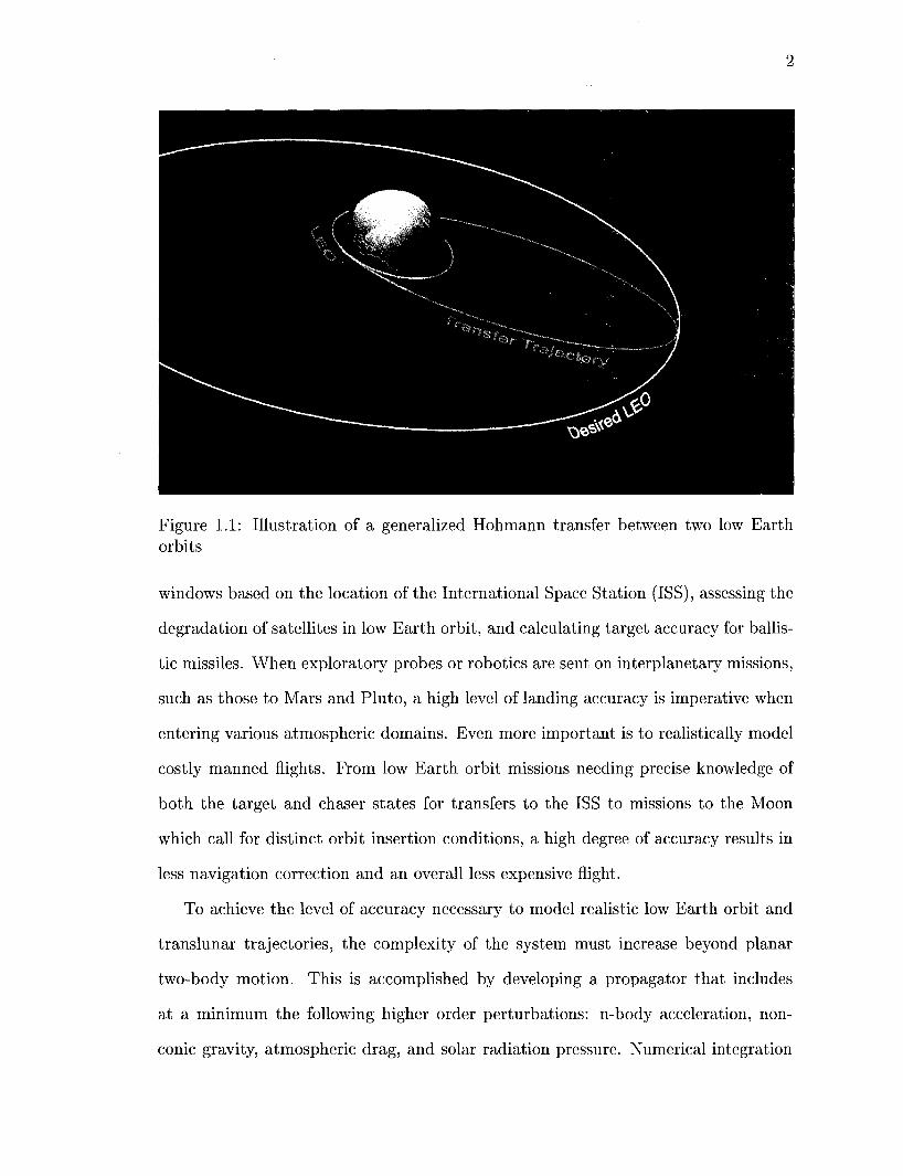
Figure 1.1: Illustration of a generalized Hohmann transfer between two low Earth orbits

windows based on the location of the International Space Station (ISS), assessing the

degradation of satellites in low Earth orbit, and calculating target accuracy for ballis

tic missiles. When exploratory probes or robotics are sent on interplanetary missions,

such as those to Mars and Pluto, a high level of landing accuracy is imperative when

entering various atmospheric domains. Even more important is to realistically model

costly manned nights. From low Earth orbit missions needing precise knowledge of

both the target and chaser states for transfers to the ISS to missions to the Moon

which call for distinct orbit insertion conditions, a high degree of accuracy results in

less navigation correction and an overall less expensive flight.

To achieve the level of accuracy necessary to model realistic low Earth orbit and

translunar trajectories, the complexity of the system must increase beyond planar

two-body motion. This is accomplished by developing a propagator that includes

at a minimum the following higher order perturbations: n-body acceleration, non-

conic gravity, atmospheric drag, and solar radiation pressure. Numerical integration

3

techniques can be utilized to account for these perturbations, however resolving the

trajectory of the vehicle to arrive at a specified target becomes a complicated task as

the motion becomes non-Keplerian.

When a high order propagator is used to determine the. final states of a trajec

tory based on initial conditions calculated from simplistic models, the predicted final

position will not match the actual propagated one. Assuming the initial position

and departure time cannot change, the transfer velocity must then be updated to fly

out a more accurate trajectory to intersect the desired final position. Utilizing linear

assumptions, the state transition matrix provides sensitivity information about the

transfer trajectory which can be used to assist in correcting the initial velocity guess

based on the error between the propagated and desired final position. Once the veloc

ity is updated the trajectory is flown out again and the position error is recalculated.

This process, known as a shooting method [8], continues until the error is within a

predefined tolerance. The transfer velocity that results from a "converged" solution

is the most accurate velocity for the fidelity level of perturbations included in the

model. The multi-functionality of this predictor-corrector method is demonstrated

by applying it to low Earth orbit and translunar cases.

The objective of this thesis is to develop an efficient, high fidelity propagator

for use in targeting and prediction applications with the capability to handle low

Earth orbit and translunar trajectories. In conjunction with low fidelity targeting

tools such as Lambert's method for low Earth orbits and Johnson Space Center's

"EXLX" for translunar trajectories (see Figure 1.2) [15], the propagator will adjust

the initial velocities predicted by the tools utilizing the correcting capabilities of a

state transition matrix. Applying a shooting method to converge on a more accurate

solution, the propagator acting as the predictor and the state transition matrix acting

as the corrector, produce a more accurate initial velocity•; required to reach a set

final position. The increased accuracy is based upon the higher order perturbation

Figure 1.2: 'Illustration of a generalized translunar transfer

models utilized by the Keplerian propagator which are not taken into consideration

by the low fidelity targeting schemes. The maximum error handling of the predictor-

corrector will be demonstrated to quantify the accuracy of the initial guess to produce

a converged solution. An additional key capability of the tool includes the output of

the trajectory states over the transfer period. These values are relevant to applications

such as navigation performance, velocity trade studies, or mission planning. Since the

output frequency of the states is configurable, the generated trajectories are beneficial

as reference trajectories in dynamic simulations as well.

The purpose of this thesis is to develop a high order propagator that can be utilized

in conjunction with an error state transition matrix to predict feasible initial states for

low Earth orbit and translunar trajectories. Chapter 2 begins with an introduction of

the classical orbital elements and Kepler's problem. It continues with an overview of

special perturbation techniques. The section covers the various perturbation methods

utilized as well as the numerical integrators chosen for this research. Chapter 2 also

5

identifies the errors that are inherent in utilizing any form of numerical integration.

Chapter 3 discusses the development of the propagator model in MATLAB to

include the perturbation models for n-body motion, higher order gravity, drag, and

solar pressure.

Chapter 4 introduces the formulation of the state transition matrix to include the

calculation of the partial derivatives for the perturbations. The accuracy of the state

transition matrix over varying times of flight and initial perturbation percentages is

demonstrated. The shooting method is also introduced.

The following two chapters demonstrate the capability of the predictor-corrector

for translunar (Chapter 5) and low Earth orbit transfers (Chapter 6). Each chap

ter tests a variety of transfers as well as the sensitivity of the algorithm to initial

perturbations.

Finally, Chapter 7 summarizes the findings of this research and makes recommen

dations for future work to include implementing a higher order propagator, utilizing

a more accurate state transition matrix, and modeling finite burn effects through the

use of two level targeting.

Chapter 2

Special Perturbation Techniques

Defining the state of a space vehicle is the first step to understanding orbital motion.

At a minimum, six quantities are required to define the state. The two most popular

representations of these quantities are the state vector which includes a position, r,

and velocity vector, v ,

r X = (2.1)

and the classical orbital element set which uses the scalar magnitude and angular

representations of the orbital elements to describe the motion. Here and for the

remainder of all equations in this paper, vectors are distinguished from scalar values

with the use of bold text. Matrices are indicated by capitalized bold text.

2.1 Orbital Elements

The six classical orbital elements are semimajor axis (a), eccentricity (e), inclination

(i), right ascension of ascending node (O), argument of perigee (ui), and true anomaly

(u) [49]. The elements, excluding a and e, are illustrated in Figure 2.1.

To understand the semimajor axis, one must look at the geometry of a conic

section. A conic section is the curve generated by the intersection of a plane and a

7

Figure 2.1: Illustration of the classic orbital elements: inclination (i), right ascension of ascending node (fi), argument of perigee (u), and true anomaly (i/) [49]

right circular cone. Based on where the plane intersects the cone, four unique conic

sections are created which represent all possible conies. These four sections make

up circular, elliptical, parabolic, and hyperbolic orbits. Every conic section has two

foci, illustrated as F and F' in the elliptical conic in Figure 2.2. In the field of

astrodynamics, the gravitational center of attraction is located at the primary focus,

F, and thus is illustrated as the center of the Earth in Figure 2.2. The semimajor

axis is half the distance of the major axis, and is used to describe the size of the orbit.

The directix is the distance from each focus to a fixed line. The ratio of the distance

of the focus from the orbit to the distance from the directix is the eccentricity. The

eccentricity of an orbit describes its shape and from Figure 2.2 is

e = - (2.2)

where c is the half distance between the foci.

5.0-

0.0-I % j *

F

-.5.0j-^-4—r— -9.0 0.0 4.0 ER

Figure 2.2: Elliptical orbit conic section illustrating the two foci, F and F', as well as the semimajor axis, (a) [49]

The distance from the primary focus to the extreme points of an elliptical orbit

are known as the radius of apoapsis, ra, and radius of periapsis, rp, which represent

the distance from farthest and nearest points respectively. The inclination, i, refers

to the tilt of the orbit plane and is the angle measured from the unit vector K and

the specific angular momentum vector, h

h = r x v. (2.3)

The right ascension of the ascending node, O, is the angle measured from the

Earth's equatorial plane to the ascending node. The ascending node is the point on

the equatorial plane at which the satellite crosses from the south to the north. For

equatorial orbits the node does not exist and thus the right ascension of ascending

node is undefined. The argument of perigee, u>, is the angle from the ascending

node to the periapsis. For circular orbits in which the periapsis is undefined and

for equatorial orbits in which there is no ascending node, the argument of perigee

9

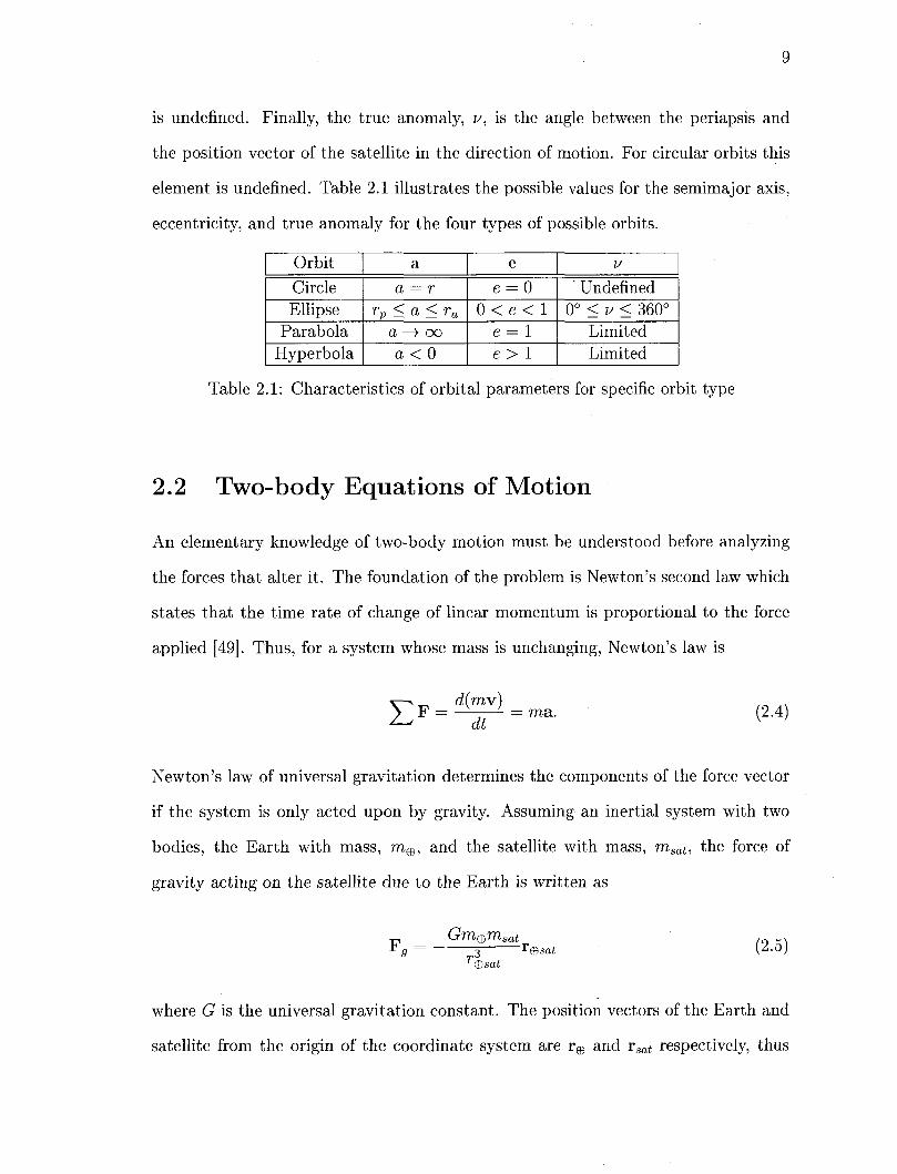
is undefined. Finally, the true anomaly, is, is the angle between the periapsis and

the position vector of the satellite in the direction of motion. For circular orbits this

element is undefined. Table 2.1 illustrates the possible values for the semimajor axis,

eccentricity, and true anomaly for the four types of possible orbits.

Orbit

Circle Ellipse

Parabola Hyperbola

a

a = r rp<a<ra

a —> oo a< 0

e

e = 0 0 < e < 1

e = 1 e> 1

V

' Undefined 0° < v < 360°

Limited Limited

Table 2.1: Characteristics of orbital parameters for specific orbit type

2.2 Two-body Equations of Motion

An elementary knowledge of two-body motion must be understood before analyzing

the forces that alter it. The foundation of the problem is Newton's second law which

states that the time rate of change of linear momentum is proportional to the force

applied [49]. Thus, for a system whose mass is unchanging, Newton's law is

v^,- , d(mv) > F = v ., ' = ma. dt

(2.4)

Newton's law of universal gravitation determines the components of the force vector

if the system is only acted upon by gravity. Assuming an inertial system with two

bodies, the Earth with mass, m e , and the satellite with mass, msat, the force of

gravity acting on the satellite due to the Earth is written as

Gm^rrisat ^sat (2.5)

Bsat

where G is the universal gravitation constant. The position vectors of the Earth and

satellite from the origin of the coordinate system are r® and vsat respectively, thus

10

the position vector of the satellite with respect to the Earth can be written as

r®sat — rsat ~ r®- (2-6)

Utilizing an inertial coordinate system, the second derivative of Equation 2.6 produces

the acceleration of the satellite relative to the Earth

X(£>sat = rsat ~ r®- (2-7)

Plugging the accelerations into Equation 2.4 and setting the results equal to Equation

2.5 gives

•"- gsat l"'satL sat T3 L sat sat

(2.8)

Solving for the individual accelerations in Equation 2.8 and substituting these values

into Equation 2.7, the relative acceleration

_ G(m@ + mBat) LiSsat — — 3 I®sat Vz-yJ

r®sat

is found. Assuming the mass of the satellite is significantly smaller than the mass of

the Earth, msat can be neglected. Furthermore, the quantity Gm® can be replaced by

the gravitational constant /i, resulting in the relative form of the two-body equation

of motion,

Y®sat = 3 r©sat- (2.10) r®sat

Equation 2.10 assumes no other forces act on the system except for gravitational

forces between the Earth and satellite. Kepler's laws, which form the foundation for

Kepler's equation, provide the necessary conditions for all two-body motion.

11

2.3 Kepler's Equation

Kepler's equation determines the relation between time and angular displacement

within an orbit. To calculate the unknown area swept out by a satellite in an elliptical

orbit, Kepler applied his second law that states equal areas are swept out in equal

times, that is At P . A1 nab v '

where P is the orbit period

P = 2TT\I—, (2.12)

with a and b being the semimajor and semiminor axes of the ellipse, and Ai denoting

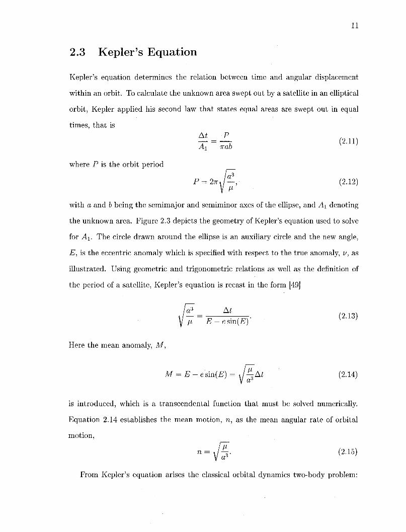
the unknown area. Figure 2.3 depicts the geometry of Kepler's equation used to solve

for A\. The circle drawn around the ellipse is an auxiliary circle and the new angle,

E, is the eccentric anomaly which is specified with respect to the true anomaly, u, as

illustrated. Using geometric and trigonometric relations as well as the definition of

the period of a satellite, Kepler's equation is recast in the form [49]

At fi E — e sin(E)'

(2.13)

Here the mean anomaly, M,

M = E-esm(E) = J ^At (2.14)

is introduced, which is a transcendental function that must be solved numerically.

Equation 2.14 establishes the mean motion, n, as the mean angular rate of orbital

motion,

n = y j . (2.15)

From Kepler's equation arises the classical orbital dynamics two-body problem:

12

Circle

c=ae

Figure 2.3: Geometry of Kepler's equation [49]

given initial states, r0 and v0, find the states r and v after an arbitrary transfer time,

At. For two-body motion there exist many analytical solutions to Kepler's problem

including using orbital elements or the / and g functions [49]. The disadvantage of

these two methods is that they are limited to specific orbit types. Following Bate

Mueller and White [6] as well as Battin [7], Vallado [49] uses elements from both

methods to present a universal formulation that is valid for all orbit types.

Vallado begins with the specific mechanical energy,

c = X° _ E K 2 r0

(2.16)

13

and defines the variable a as - v 2 2

a = ^ o + ± . (2.17)

Here a is used to avoid calculating the eccentricity to determine the orbit kind in the

initial guess. Depending on the value of a , different algorithms are used to calculate

the universal variable, %. If the orbit is circular or elliptical (a > 0.000001), the

variable is approximated as

Xo « y/JI(At)a. (2.18)

For parabolic orbits (a < 0.000001) the specific angular momentum h = r0 x v0 is

calculated, to find the semiparameter, p,

h2

p=-. • (2.19) .A*

The values are needed to solve for the angles w a n d s in Barker's equation

cot(2s) = 3, /4-(At) • (2.20) V P

tan3(w) = tan(s) (2.21)

and are used to approximate the universal variable

X~ ^/p2cot(2w). (2.22)

Finally, if the orbit is hyperbolic (a < —0.000001), the semimajor axis is defined as

a = - and a

14

Next the variable ip is defined as

V> = Xl® (2.24)

and used to calculate a family of functions, c2 and c3; if ip > 1 x 10~6,

1 - cos (Vff) ^ - sin ( y ^ ) 2 - ^ 3 ~ 7? ' ( }

if ip < - 1 x 1(T6,

^ = 1 - cosh ( y ^ Q c s = s i n h ( V ^ - y ^ ^

and in all other cases c2 = | and c3 = | . The function values are used in the position

equation

r = X2nC2 + ^ T ^ X n (1 - V>c3) + ro (1 - Vc2) (2.27)

which updates the universal variable

Xn+l = Xn + ~ ^ • (2.28)

The value of Xn+i replaces the previous value of Xn and Equations 2.24-2.28 are

iterated until \xn — Xn+i\ < 1 x 10 -6 . Defining the / and g functions as

/ = ! - — c 2 , (2.29)

with

and

/ = — Xn (ipc3 - 1); (2.30) rr0

9 = At-^c3, (2.31)

15

with

g = 1 - ^ c 2 (2.32) r

the final position and velocity vectors are calculated using the equations

r = / r 0 + <?v0 (2.33)

v = / r 0 + <?v0. (2.34)

This general formulation analytically predicts orbital states for any satellite motion

about a central body. However, in actual spaceflight additional forces act causing

significant perturbations from the Keplerian trajectory. Unfortunately no closed form

solutions to these perturbed equations of motion are known to exist and as a result

they must be solved numerically. The following section will discuss the development of

equations of motion that include dominant perturbations and the numerical methods

that are commonly used to find solutions for the general problem.

2.4 Equations of Motion with Perturbations

Disturbing accelerations from non-Keplerian effects such as the gravitational attrac

tion of other planets, the non-spherical shape of the Earth, atmospheric drag, and

even solar radiation cause deviations from the conic two-body trajectory presented in

Section 2.3. As a consequence of these deviations, the two-body equations of motion

are insufficient to accurately solve trajectory problems. The magnitude of a pertur

bation does not need to be large to greatly affect a trajectory. For example, over time

the trajectory of a satellite in low Earth orbit will drift due to the oblateness of the

Earth. If the effects of this uneven mass distribution were ignored in planning the

initial trajectory, the satellite's orbit could degrade until the vehicle burned up in the

Earth's atmosphere.

16

Perturbation analysis has played an important role throughout history in the

study of celestial bodies. In 1619, Johannes Kepler theorized that comet tails were

pushed outwards from the Sun due to pressure from sunlight; a theory that is quali

tatively the same as our current view of solar radiation pressure [32]. At the end of

the 18th century Pierre-Simon Laplace made significant developments to the mod

eling of Earth's gravitational field with his contribution to the potential function.

Additional progress into the gravitational-potential problem was made in 1783 when

Adrain Marie Legendre published his solutions to differential equations arising from

his studies on the attraction of spheroids. In 1849, Sir George Gabriel Stokes pub

lished a formula which determined the shape of a geoid based on the known local

gravity anomalies [49]. E.M. Brown's papers of 1897-1908 explained the perturbative

effect of the oblateness of the Earth and Moon on the Moon's orbit. In the mid-

19th century the English astronomer John Couch Adams and the French astronomer

Urbain-Jean-Joseph Le Verrier separately used the method of variation of parameters

to study the irregularities of the motion of Uranus. Their observations and calcula

tions eventually led to the discovery of the new planet Neptune which was the cause

of the deviations in Uranus's orbit. Calculating the perturbations caused by Jupiter

and Saturn, Alexis Clairault made the first accurate prediction of the return of Hal-

ley's Comet in 1759 [6]. These few examples underline the necessity of including

perturbations in targeting and prediction analysis.

There are two approaches to solving equations of motion with perturbations: the

"general perturbation" approach and the "special perturbation" approach. The general

perturbation technique is an analytical expansion and integration of the equations of

variations of orbit parameters. The special perturbation process is a step-by-step

numerical integration. Though the general perturbation approach will be briefly

reviewed, the research of this thesis relies upon a basic special perturbation process

known as Cowell's method.

17

2.5 CowelPs Method

Cowell's method is a step-by-step numerical integration of the two-body equations of

motion, including a general disturbing acceleration term [17]. The equation of motion

to include the disturbing "perturbing" accelerations is

r + ^ r = ap, (2.35)

where [i is the gravitational constant of the central body and a , is a linear combination

of all the perturbation accelerations. For numerical integration Equation 2.35 is

reduced to the first-order system of differential equations

r = v (2.36)

and

v = - ^ r + ap. (2.37)

Cowell's method has many advantages, the foremost being its simplicity of formulation

and implementation. The method is most efficient if ap is of the same order of

magnitude or higher than the dominant gravitational acceleration. If ap is small the

method becomes inefficient as smaller integration steps must be taken to maintain

accuracy which results in an increase in computation time and accumulative error

due to roundoff [7]. Roundoff and truncation error will be discussed in further detail

in Section 2.8.1. One way to slightly mitigate the error is to apply Cowell's method

with polar or spherical coordinates instead of the classically implemented Cartesian

coordinates [6]. With these coordinate systems, the radius from the Earth to the

vehicle, r, tends to vary slowly and the angle change is always monotonic. This allows

larger integration steps, and thus less computational time, for the same truncation

18

error. The equations of motion in spherical coordinates (r,6, 4>) are:

r - r (o2 cos2 4> + 4>2 J = - ^

rO cos 4> + 2r# cos <p — 2r9<j) sin 0 = 0,

where the angles (9 and 4> are defined in Figure 2.4.

(2.38)

Figure 2.4: A representation of a spherical coordinate system [53]

Depending on the trajectory, a^ can be orders of magnitude smaller then the dom

inant gravitational force. This occurs in low Earth orbit where the effect of Earth's

oblateness is three orders of magnitude smaller then the spherical gravity acceleration

[43]. In other words, looking at Equation 2.37, the two-body term,—-^, has a much

larger value then a^. Though Cowell's method will accurately integrate the effects of

all the accelerations, it does not consider the benefit of integrating the perturbation

separately from the two-body term. Since the two-body term dominates, most of the

computational time will be spent integrating this piece. However, since an analytical

solution exists for the two-body equations the expensive numerical integration of the

dominating term can be avoided. Encke's method, which is another basic scheme in

the special perturbation category, takes advantage of this benefit. As a result, Encke's

19

method requires fewer integration steps over a specified At to get the same accuracy

as Cowell.

2.6 Encke's Method

Whereas Cowell's method integrates the sum of all the accelerations, Encke's method

integrates the difference between the primary gravitational acceleration and all per

turbing accelerations. Encke's method begins with an "osculating orbit" which is the

conic path the orbit would make if no disturbing acceleration exerted an influence on

the vehicle (see Section 2.2). However, the true motion of the vehicle will not take

place along the osculating orbit, but will differ from the associated position in the

conic orbit by an amount corresponding to the central body force. This concept is

utilized to calculate the perturbed orbit [42].

At time to, the perturbed orbit is equal to the osculating orbit,

r = rosc v = vosc. (2.39)

At some time later, t = to + At, the perturbed orbit has moved away some distance,

Sr, and velocity, 5v, from the osculating orbit. See Figure 2.5 for clarification, where

Sr = S(t). Thus at any time, the position and velocity vectors of the true orbit are

given by the vector sum of the two-body and perturbed components. Specifically,

r = rosc + Sr v = vosc + Sv. (2.40)

20

f(tQ)

osculating reference

orbit

actual perturbed ^ orbit

Figure 2.5: Vector definition for Encke's method [43]

To calculate 8r, start with the two-body and perturbed accelerations

V A* (2.41)

where once again ap denotes the perturbation acceleration vector. The difference

between the two types of orbital motion satisfies the differential equation

<5f = aB + V

osc 1 r — <5r >. (2.42)

It is difficult to accurately calculate the coefficient of r because Equation 2.42 essen

tially takes the difference of two nearly identical numbers resulting in roundoff error.

This obstacle is circumvented by employing the approximate technique set forth by

Battin [7]. Specifically,

r = TOSC + 5v (2.43)

thus one can write that

= -f(q) = l-(l + q)>, (2.44)

21

where Sr • (Sr - 2r) • ,

q = - L. (2.45) r • r

The function f(q) can be written as

™ = <TTKT7' (2'46)

1 + (1 + q)2

thus, the deviations from the osculating orbit are calculated in the equation

Sv = ap - 4 - (f(q)v + ST) . (2.47) osc

Integrating the value produced from Equation 2.47 once results in 5v, integrating

a second time produces <5r, both values which are needed in Equation 2.40 at each

propagation interval.

2 . 6 . 1 R e c t i f i c a t i o n

The terms in Equation 2.47 must remain small in order for Encke's method to remain

accurate. As the deviation vector, ST, grows in magnitude, the acceleration term

increases as well. To maintain efficiency, the osculating orbit must be re-initialized, a

process known as rectification. At rectification the osculating orbit is set equal to the

true position and velocity vectors and the initial conditions Tor Equation 2.47 are set

to zero so that the only acceleration felt by the vehicle is ap. The rectification point

is set to occur at every pass or a set tolerance depending .on the desired algorithm.

Rectification ensures the control of numerical errors. . Calculation of the conic

orbit results in only roundoff errors and is independent of the numerical technique

utilized to perform the integration. However, calculation of the deviations from the

osculating orbit result in both roundoff and truncation error due to the finite number

of steps performed by a particular numerical algorithm. As the orbit is propagated,

22

truncation errors will increase for each step. To prevent these errors from growing

large enough to have a detrimental effect, rectification resets the osculating orbit [7].

To compare the relative accuracy of CowelPs method to Encke's method, 7,000 low

Earth orbits with various orbital elements were propagated over one period assuming

two-body motion. The final position vectors were compared against the analytical

solution to Kepler's problem as discussed in Section 2.3. The statistical information

of the magnitude error for both methods is represented by a boxplot in Figure 2.6.

For all boxplots in this research, the bottom and the top of the box represent the

25th and 75th percentile, or the lower and upper quartiles respectively. The red band

near the middle of each box is the 50th percentile, or the median. The middle 50%

of all the information collected falls within the boundaries of the box. The whiskers

represent the lowest datum within 1.5 interquartile range of the lower quartile and

the highest datum within 1.5 interquartile range of the upper quartile. Data outside

of the whiskers is plotted as an outlier with a small circle.

For this comparison, Encke's method utilized a variable step Nystrom integration

scheme whereas Cowell applied a variable step Runge-Kutta method. The integration

schemes were selected based on tool availability. Both of these integration techniques

are discussed in Section 2.8. The difference in integration methods will produce

slightly different results in the final propagated states. The purpose of the comparison,

however, is not to illustrate the benefit of one method over the other but to show

how both produce relatively similar errors. From Figure 2.6 the similarity in median

error between Cowell's and Encke's method is apparent, with 0.02 km and 0.09 km

respectively. Outlier points for Cowell's method are indicative of highly elliptical

orbits which have much longer periods. The trend of increased error over longer

propagation times is an expected behavior of numerical integration and is discussed

in Section 2.8.1. Errors in Encke's method are a result of the different algorithms used

by the integration scheme and the truth value to compute the Keplerian solution. If

23

Magnitude Difference Between Final Position of CowelJ and Encke Propagation and Kepler's Analytical Solution for 7000 Low Earth Orbits Over One Period

1 1 e

1

•

-

'•

-

i

;

:

-

-

I I

Cowell's Method Encke's Method

Figure 2.6: Boxplot comparison of the magnitude difference in final position of Cow-ell/Encke propagation and Kepler's analytical solution for 7,000 low Earth orbits over one orbit period

the same analytical algorithm was applied to both Encke's method and the truth case,

Encke's method would produce zero error. From the 7,000 cases tested, depending

on the orbit type, Encke's method took 2-3 times fewer steps then Cowell's method.

Similar results are found in Reference [4]. Though Encke's method has the advantage

of accuracy and computational time, Cowell's method is relatively simple to code

and performs comparably to Encke's method. For this reason, Cowell's method was

selected as the perturbation method used in this research.

2.7 Variation of Parameters

The method of variations of parameters was developed by Euler in 1748 and improved

by Lagrange in 1873. It was the only successful method of perturbations until the

development of Cowell's and Encke's method in the early 20th century. In terms of

24

the process of rectification as discussed in Encke's method, the variation of parameter

method can be viewed as a continuous rectification of the osculating orbit at each

instant of time. Thus the "reference" orbit is constantly changing. Any two-body orbit

can be completely described by a set of six orbital elements, however in the perturbed

problem these elements become time varying parameters. The purpose of the variation

of parameters method is then to determine how the parameters change with time as

a result of some perturbing force [14]. Analytically integrating the expressions for the

time changing orbital elements is the method of general perturbations. Due to the

fact that the elements will change much more slowly then their position and velocity

counterparts, larger integration steps may be taken.

From a coding stand point, the variation of parameters method is the most difficult

to implement of the methods discussed thus far. For this reason, again Cowell was

chosen as the preferred method to use.

2.8 Numerical Integration Methods

Special perturbations require a form of numerical integration in their implementation.

No matter how complex the analytical foundation of a special perturbation technique

may be, the results are worthless after integration if an appropriate integration scheme

is not selected. The following is a discussion on the errors inherent in numerical

integration as well as the numerical methods utilized in this research.

2.8.1 Integration Errors

In numerical integration there are two main types of errors involved: roundoff errors

and truncation errors. Roundoff error is due to the finite precision, or floating point

arithmetic implemented by computers. Computers are only accurate up to a certain

number of digits. This number, rj, is the smallest number which when added to a

25

number of order unity gives rise to a new number. Every floating-point calculation in

curs a roundoff error of order 77. For instance, if a computer could only carry up to five

digits and the following numbers were added together: 123.456 + 789.012 = 912.468,

the computer would round the answer to 912.47. Where the actual answer has a 6 in

the fifth digit, the rounding error has resulted in a 7. Over time, this accumulation

of roundoff error will result in a much larger error. Brouwer and Clemence developed

the formula

log (.1124ns) (2.48)

to illustrate the probable error in terms of number of decimal places after n steps have

been taken [9]. Thus, for an integration scheme that took 500 steps the error would

be around 3.1 decimal places. If 6 places of accuracy are required then 6 + 3.1 « 10

places are required to carry out the calculations. Though modern computers have a

value of r\ = 2.2 x 10~16 for double precision floating point numbers, it is clear that

integration schemes that require less steps will inherently incur less roundoff error.

Where roundoff error is typically a result of the machine used to handle the calcu

lations, truncation error is a function of the numerical integration method selected.

Truncation error results from the inexact solution of the differential equations. As

discussed in the following section, numerical methods are derived from some form of

the Taylor series expansion. Since not all of the series are utilized, the methods are

forced to truncate or exclude higher order terms, and a truncation error develops.

Thus, the larger the step size the larger the truncation error.

Truncation error can be assessed from two points of view: local and global. Local

error is the error that would occur in one step if the values from the previous step

were exact and there was no roundoff error [33]. Assume un(t) is the solution of a

differential equation calculated from the value of the computed solution at some time

tn and not from the original initial conditions at t0. Thus un(t) is a function of t

26

defined by the equations

iin = f (t, un) K ' (2.49)

l^n V'n) = Vn-

The local error, dn, is the difference between the theoretical solution and the computed

solution calculated using the same information at tn. That is,

dn = Vn+i - un (tn+1). (2.50)

Global error, on the other hand, is the difference between the computed solution and

the true solution determined from the original conditions at time to,

en = yn-y (tn) • (2.51)

For the case where a function f(t, y) does not depend on y, the global error becomes

the sum of the local errors. In most cases, however, f(t, y) does depend on y and thus

the relationship between global error and local error is related to the stability of the

differential equation. For a single scalar equation, if the sign of the partial derivative

is positive, the solution y(t) grows as t increases and the global error will be greater

then the sum of the local errors. The opposite trend is true as well: a negative partial

derivative will result in a larger local error then global error. All of the MATLAB

solvers used in this research only attempt to control the local error. Solvers that try

to control global errors are much more complicated and rarely successful.

A measure of accuracy of a numerical method is its order. The order represents

the local error that would occur if the numerical method were applied to problems

with smooth solutions. A method is of order p if there is a number C such that

\dn\ < Chp+1 (2.52)

27

where n is the step number and h is the step size. The value of C can depend on

the derivatives of the differential equation and on the length of the interval but it is

independent of n and h. A popular abbreviation of Equation 2.52 is the notation

dn = 0{h?+l), (2.53)

which will be used to discuss the accuracy of various numerical methods in the fol

lowing section.

2.8.2 Euler's Method

There exist many numerical methods to approximate the equations of motion used

in astrodynamics. For the purpose of this thesis the focus will remain on single-step

methods for numerical integration problems. Single-step methods take the state at

one time with the rates at several other times, based on the single-state value at time,

to. The rates are obtained from the equations of motion and are used to determine

the state at succeeding times, t0 + h. Most numerical integrators are based on the

integration of the Taylor series

V(t) = V M + V fa) (t - t0) + * M [t2~ *•>' + » ' ( * • > % - ^ + . . . (2.54)

However, in this format two major issues arise. The first is after which order should

the series be truncated. The second issue is how to calculate the higher order deriva

tives. Taking the most basic approach to both these issues results in the Euler inte

grator which approximates the Taylor series to the first order [28]

y(t)~y{t0) + f(t0,y0)(t-t0). (2.55)

28

This method is simplistic in that it only requires knowledge of the first derivative but

it is unsymmetrical in that it attempts to determine the slope only at the starting

point. The major disadvantage of Euler's method is its sensitivity to step size, defined

here as h = t —10. The method assumes the domain is linear, and the chosen step size

is small enough to handle variations caused by the neglected higher-order derivatives.

However situations can arise where the states change drastically between step sizes

in which case the Euler method will provide very inaccurate solutions. The error

associated with Euler's method is illustrated by Taylor expanding y(t) about t = to,

h2

y (t0 + h)=y (t0) + hy (t0) + —y (t0) + ... (2.56)

h2

y(t0 + h) = y (to) + hf (t0, y0) + —y (t0) + ... (2.57)

A comparison of Equations 2.56 and 2.57 illustrates

V(t) = V (to) + hf (t0, y0) + O (h2) . (2.58)

Thus, each step using Euler's method incurs a local truncation error on the order of

0(h2). Additionally, from Equation 2.53 it is clear that p = 1, so Euler's method

is first order. The Runge-Kutta methods provide a more accurate scheme to handle

complex problems.

2.8.3 Runge-Kutta Method

The Runge-Kutta method also derives from the Taylor series. However, instead of

having to derive formulas for the higher order derivatives, the values are approximated

by integrating the slope at different points within the desired interval. One option

is to take a similar approach as Euler's method by obtaining the initial derivative

at each step, but this time the derivative is used to find a point halfway across the

29

interval. The value of both t and y at the midpoint are then used to compute the

actual step across the whole interval. This is the second-order Runge-Kutta method,

also known as Heun's method,

Vi = f(t0,y0)

fc = /(*o + ii/b + f»i) (2-59)

y(t) = y (to) +1 (in + m) + O (hs).

As evident from the error term, the symmetrization of the second-order Runge-Kutta

method is accurate up to the second-order with a truncation error of the third order.

The most often used variation of the Runge-Kutta methods is the classical fourth-

order Runge-Kutta method,

yi = f(to,yo)

h = f {to + f, yo + |yi)

ys = f(to + l,y0 + ly2) (2-60)

2/4 = / (*o + h,y0 + hy3)

y(t) = y (t0) + | (yx + 2y2 + 2y3 + y4) + O (h5).

The method is derived from a fourth-order Taylor series expansion about the initial

value y(to). Equation 2.60 negates the need for higher order time derivatives by

relating them to first derivatives at different times. The fourth-order Runge-Kutta

uses the weighted averages of four slopes to then determine the next step. The method

has fifth-order local truncation error and fourth-order global truncation error. A

comparison of the three methods discussed is shown in Figure 2.7.

30

Euler's Method

>'i

t ^ t o + h t 2 = t!+h

RK Order Method

>!2

to to+h/2 t j t i+h/2 t2

RK 4* Order Method

>'3 >'4

>'l X y%

tc+h/2 tj+h

Figure 2.7: Comparison of Euler's Method, second-order Runge Kutta method, and fourth-order Runge-Kutta method where the black dots represent the estimated values and the red dots are the intermediate points

31

2.8.4 Nystrom Integration Method

Where the Runge-Kutta integration methods utilize the first order form of the equa

tions of motion, y = f(t,y), the Nystrom method requires the second order form

y = f(t,y). (2.61)

The method gives fourth-order accuracy while requiring only three derivative com

putations per time step. This is an advantage over the Runge-Kutta method which

requires four derivative computations. Thus, in situations where the equations of

motion can be expressed in second order form, the Nystrom method will be more

accurate and efficient then Runge-Kutta. The second order system is written as

(2.62) y = v

y = v = f(t,y).

Where the formulas are of the form

V\ = f(t0,y0)

y2 = f{t0 + l,yo + vo + fy^j

3/3 = / (to + h,y0 + hv0 + f ij2) (2.63)

V(t) = y (t0) + hv (t0) + f (Vl + 2y2) + O (h5)

v(t) = v (t0) + l(yi+ Ay2 + y3) + O (h5) .

As previously mentioned, the Nystrom method requires equations of motion in the

second order form. If the equations include velocity, the second derivative of velocity,

known as jerk, must be calculated. In order to avoid this complexity, the Nystrom

formulation assumes the equations of motion are independent of velocity, thus the

32

acceleration due to drag is not included in the traditional Nystrom formulation,

y = f(t,y)^f(t,y,y). (2.64)

D'Souza developed a modified Nystrom formulation that can handle the velocity term

[20],

V\ = f(to,yQ,vQ)-

2/2 = (to + f, yo + %v0 + YVUVO + |y i )

i/3 = f (t0 + h,yo + hv0 + ^y2,v0 + hy2y (2.65)

y(t) = y(t0) + hv(t0) + ^(yi + 2y2) + O(h5) '

• v(t) = v(to) + %(yi + 4y2 + m) + 0(h5).-

Analysis done on this modified formulation illustrates it is as accurate as the Runge-

Kutta algorithm for fewer function evaluations.

2.8.5 MATLAB Solvers

All numerical integration for this thesis is performed using MATLAB's built in solvers.

The available variable-step solvers for non-stiff systems with their specific integration

techniques are listed in Table 2.2. Unlike a fixed-step solver which maintains a con

stant step size, a variable-step solver varies the step size depending on the dynamics

of the model and the error tolerances specified by the user. This ability enables the

solver to increase the step size where necessary and thus reduce the total number of

steps needed. Minimum and maximum step sizes can be set as well if constraints

are required. The ode23 scheme implements the Bogacki-Shampine method which

uses a Runge-Kutta formula of order three with four stages with the first-same-as-

last (FSAL) property. As a result, it uses approximately three function evaluations

per step. This method is a single-step method because only information from the

previous point is needed to compute the successive point. The ode45 scheme is an

33

explicit Runge-Kutta(4,5) formula that uses the Dormand-Prince method of applying

six function evaluations to calculate the fourth and fifth order accurate solutions. The

difference between the solutions is the error of the fourth order solution. Like ode23,

ode45 is a single-step solver. The ode 113 scheme is a variable order Adams-Bashforth-

Moulton multi-step PECE solver. PECE is a technique of handling ordinary differ

ential equation approximation by taking a prediction step and single correction step.

The "E" in the acronym refers to the evaluations of the derivative function. Unlike

ode45, ode 113 is not self starting and thus requires solutions from four preceding

time points to compute the current solution [1].

Solver ode23

ode45

ode!13

Integration Technique Explicit Runge-Kutta (2,3) pair of Bogacki and Shampine One-step solver Explicit Runge-Kutta (4,5) pair of Dormand-Prince One-step solver Variable order Adams-Bashforth-Moulton Multi-step PECE solver

Table 2.2: MATLAB fixed-step continuous solvers

To illustrate the performance of MATLAB's numerical integrators, a circular equa

torial orbit was propagated for one period using a variety of tolerances. In MATLAB,

the relative tolerance is a measure of the error relative to the size of each solution

component. It controls the number of correct digits in all solution components [1].

The default value is 1 x 10 -3, corresponding to 0.1% accuracy. The measures of per

formance used to compare the integrators were computation time, number of steps

taken, and error. The computation time was calculated using MATLAB's "tic toe"

functions placed before and after each solver integration. The number of steps each

solver took was determined by the length of the output vector. The error of the

integrators was based off the magnitude difference of the final position vector after

propagation and the analytical two-body Kepler solution. The results are plotted in

Figures 2.8-2.10.

34

Figure 2.8 highlights the relative similar performance of all three solvers at very

low tolerances. As the tolerances increase however, the lower order solvers require

much more computational time. At a tolerance of 1 x 10~13, ode23 takes more than

37 times the amount of time as required by ode 113. In comparing the number of

steps the solver takes to maintain the specified tolerance as depicted in Figure 2.9, it

is clear the advantage ode45 and ode 113 have over the lower order ode23. Even at a

tolerance as low as 1 x 10~4, ode23 takes three times the number of steps as ode45.

Figure 2.10 depicts a relatively similar error performance for all the solvers across

all tolerances. More importantly, the figure illustrates the importance of selecting

sensitive tolerances (> 1 x 10~6) for even the highest order solvers in order to achieve

a level of accuracy. As a result of the performance demonstrated in Figures 2.8-2.10,

only MATLAB's ode45 and ode 113 were utilized in this research.

With the background of perturbation techniques and numerical methods just dis

cussed, the next chapter develops the propagation model used as the "predictor" for

the predictor-corrector algorithm applied in this study.

Comparison of Computation Time Between MATLAB ODE Solvers 10

10' In 0)

F10° to c o

•g 10 a. E o O

10 .-2!

10 -3

ode23 ode45 \ -ode113

10 -15 10"1 0 I * 5 '

Tolerance 10"

Figure 2.8: Comparison of computation time between MATLAB's ODE solvers

35

of Number of Steps Taken MATLAB ODE Solvers

Tolerance

Figure 2.9: Comparison of required number of steps between MATLAB ODE solvers

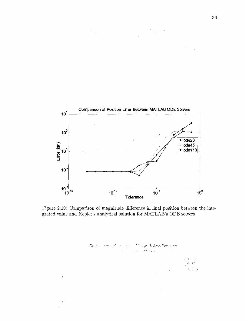
Comparison of Position Error Between MATLAB ODE Solvers •»4

Tolerance

Figure 2.10: Comparison of magnitude difference in final position between the integrated value and Kepler's analytical solution for MATLAB's ODE solvers

Chapter 3

Development of Propagator

3.1 System Overview

At initialization, the Cowell propagator requires the epoch state of the vehicle. Using

the position and velocity of the spacecraft, the propagator calculates the total pertur

bation acceleration, ap from Equation 2.35, in five main blocks of code. Three Body

Motion computes the perturbations due to n-bodies, High Order Gravity calcu

lates the affects of non-conic gravity due to the Earth, High Order Gravity Moon

calculates the affects of non-conic gravity due to the Moon, Atmospheric Drag de

termines the acceleration due to drag, and Solar Pressure measures the affects of

solar radiation pressure. All the perturbations are summed and added to the 2-

body equation of motion as defined in Equation 2.10 to produce the final acceleration

for integration. Figure 3.1 portrays this configuration of the Cowell propagator and

highlights which section in the following chapter each perturbation acceleration is

examined.

37

38

•

r

'—'

V

Three Body Motion (Section 3.2)

High Order Gravity: Earth

(Section 3.3)

High Order Gravity: Moon

(Section 3.3.2)

Solar Radiation (Section 3.5)

Atmospheric Drag (Section 3.4)

+

+

+

+

+

«P

r3

t

1 f 1 •I r

Figure 3.1: Configuration of the Cowell propagator

3.2 Three Body Motion

Using Newton's second law and the law of gravitation the acceleration of n-bodies

acting on a spacecraft is calculated as [49],

rlso,t G 7 v""J i=3

m-i 1 satj

satj

(3.1)

Here the subscript, 1, represents the primary body which is the celestial body whose

sphere of influence is acting on the spacecraft at any one time. The index, j , references

the additional bodies included. The variable m,j is the mass of each respective planet.

The left-hand term of Equation 3.1 represents the direct-effect of the acceleration of

the third body on the vehicle. The right-hand term is called the indirect-effect because

it is the force of the third body on the Earth. Note the two-body acceleration term of

39

the Earth acting on the vehicle, — -^r, is not included because the Cowell propagator

handles the term separately (see Figure 3.1).

At high altitudes, lunisolar perturbations induce secular variations in eccentricity,

inclination, ascending node, and argument of perigee. The Sun induces a gyroscopic

precession of the orbit about the ecliptic pole, specifically a regression of the nodes

along the ecliptic. The Moon causes a regression of the orbit about an axis normal to

the Moon's orbit plane, which has a 5° inclination with respect to the ecliptic plane

with a node rate of one rotation in 18.6 years [14]. The equation of nodal regression

due to lunisolar perturbations is ,

• 3n5[l + (3/2) e2] , 9 x , x ^Body = - - ^ - - ^ U ^ c o s i (3cos2i3 - 1 (3.2)

o n \J\ — eA

and for argument of perigee is

3 n j [ l - ( 3 / 2 ) s i n 2 z 3 ] fn 5 . 2 e 2 \

^ = 4 ^ VI - e * I 2 " 2S m +V (3"3)

where 71.3 and i$ are the mean motion and inclination with respect to the Earth

equatorial plane. In order to calculate the perturbation effects of additional celestial

bodies, the planet positions at specific times with respect to a single reference frame

are required. For this research, all ephemeris data was collected from the SPICE

program.

3.2.1 SPICE

SPICE is an information system built by the Navigation and Ancillary Information

Facility under the direction of NASA's Planetary Science Division to assist engi

neers in the design of planetary exploration missions. The SPICE system produces

data sets known as kernels which contain navigation and ancillary information such

as planet ephemerides. The acronym SPICE loosely stands for the kernel file con-

40

tent: Spacecraft ephemeris, Planet location, Instrument Description, C-matrix, and

Events. In order to utilize the n-body equations of motion for this research, SPICE

returns the necessary states of the target body. The ephemeris program handles

up to 11 bodies to include the Sun, nine planets, and the Moon. The output can

be expressed in several reference frames to include planet-centered and barycentric.

Documentation on the specifics of the program can be found in Reference [3]. All

ephemeris data is time specific, thus, the correct time scheme must be utilized. The

following section details the method to convert to the time reference used by SPICE.

Time Conversion

Given the Gregorian calender date for a desired epoch time, SPICE requires a time

conversion to seconds since J2000. This calculation first requires determining the

Julian Date based on the Roman calendar. The Roman calendar starts with March

as month 1, April as month 2 and continues through February as month 12. The

equation

MR = l + (mod((MG-3),12)), (3.4)

converts the Gregorian month into the Roman month, where MR refers to the Roman

month, MG is the Gregorian month, and mod is the modulus after division. If the

Roman month is greater than 10 (either January or February), the Gregorian year

is set to one less then the entered year due to the fact that January and February

are the start of a new year. Next the number of Julian Days until March 1 of the

year of interest is calculated, taking into account leap years. The three criteria that

determine leap years are:

1. Every year that is divisible by four is a leap year;

2. of those years, if it can be divided by 100, it is NOT a leap year unless

3. the year is divisible by 400.

41

The third criterion refers to the Gregorian 400 year cycle, which occurs when the

same weekdays for every year are repeated. The Julian Day is computed using the

following algorithm:

First, consider the 400 year cycle. During this period there are 146,000 days and

97 leap years hence the coefficient 146, 000 + 97 = 146, 097,

JD = JD + 146,097(fix(Y ears/400))

Years = mod(Y ears, 400),

where the fix command rounds towards zero. Next consider the 100 year period which

includes 36,500 days and 24 leap years,

JD = JD + 36, 524(fix(Years/100))

Years = mod(Years, 100).

The 4 year period has 1,460 days and 1 leap year,

JD = JD + 1,461(fix(Years/4))

Years = m.od(Years,4).

(3.6)

(3-7)

Finally, the one year period has 365 days and no leap years,

JD = JD + 365(y ears). (3.8)

Next the number of days until the month of interest is calculated, adding this value

to the days found in Equation 3.8. These two values are added to produce the final

Julian Day value. The Gregorian hour, minute, and seconds are all converted to

seconds, added together, then converted back into days to complete the Julian Date.

42

Since SPICE utilizes a J2000 epoch, the Julian Date is converted as follows

JDJ2000 = {JD - 2,451, 545)86,400, (3.9)

where 2,451,545.0 is the Julian Date of January 1, 2000 at noon and 86,400 is the

number of seconds in a day.

3.3 High Order Gravity

The High Order Gravity model computes the gravitational perturbation accelera

tion vector due to a rotating non-spherical body whose mass coefficients are given in

terms of the zonal and tesseral harmonics. Gravity harmonics are derived from the

gravity potential which will be explained in the following section. Zonal harmonics

occur where the dependence of the gravity potential on longitude disappears and the

the field is symmetrical around the pole. These harmonics reflect the Earth's oblate-

ness as seen in the shaded regions of Figure 3.2. The gray areas highlight additional

mass, thus the central band of J2, seen as degree 2 order 0 in the figure, clearly cap

tures the bulge of the Earth. Tesseral harmonics on the other-hand take into account

the latitudinal and longitudinal effects of the mass distribution dividing the Earth

into a checkerboard (see Figure 3.3). The High Order Gravity function allows the

user to specify the order of perturbation from spherical (no perturbation due to a

non-spherical Earth), the "zeroth" order terms J2, J2J3J4, or higher order of gravity

which includes the tesseral harmonics. The mathematical formulation discussion in

the follow section assumes that the primary body of interest is the Earth.

43

Side

Top

Figure 3.2: Illustration of the Earth's zonal harmonics with shaded regions representing additional mass [49]

3,2 4,1 4,2

43

Figure 3.3: Illustration of the Earth's tesseral harmonics with shaded regions representing additional mass [49]

3.3.1 Formulation

Spherical

When the simplified gravitation potential of the Earth is utilized it assumes a spher

ically symmetric mass body which results in Keplerian motion. For this case, no

perturbations are calculated. However, the Earth is not a spherically symmetric

body but is bulged at the equator, flattened at the poles and is generally asymmetric.

These are modeled iri the following sections.

44

The most commonly encountered gravity harmonic is J2 which is the largest magni

tude term of the zonal harmonics. As the coefficient of the second harmonic, J2 is

related to the Earth's equatorial oblateness. The estimated difference between the po

lar radius and the equatorial radius due to the bulge is 22 km [14]. The accelerations

due to the second harmonic are determined using the equations

_ 3J2nR%rx f _ 5 r | U/J2,x — 2 r 5 I r 2

_ 3J2tnR^ry (^ 5 r 2 ' aJ2,y ~ 2r 5 (i-3)

and

(3.10)

Where for the Earth, J2 has the coefficient value

J2 = -1.08262668355 x 10"3, (3.11)

H is the gravitational parameter, RQ is the equatorial radius of the Earth, r =

[ rx ry rz] a r e the position vector components, and r = |r| is the magnitude of

the position vector. It is assumed r is in an Earth-Centered Earth-Fixed coordinate

frame where z is the North Pole and x is at the zero longitude.

J2J3J4

Though the J2 coefficient is almost 1000 times larger than the next largest coefficient,

J3, multiplying J2 by J3 and J4 increases the accuracy of the predicted perturbation.

The accelerations due to the second, third, and fourth harmonic utilizes Equation

45

3.10 added to the equations

_ 5J3»R%rx f _ 7rf.

_ 5 J 3 / i i i | r y / „ _ 7 r l \ aJ3,V — 2r7 \ °'z r2 1 i

(3.12)

and hJ^R%rz /r _ 7rJ _ 3rJ

2r7 I r2 5 r aJ3,* = 7^ I 6rz

for the third harmonic and to the equations

_ 15J4liR^rx A _ I 4 r | . 21r4

aJi,X — g r7 I J- r2 ~T rA

_ _ 1 5 J 4 ^ R | r E / _ I 4 r | 21r£ a J 4 , y ~~ 8r 7 ^ r 2 ~T~ r 4

and 15J4^i?®r:r / 70r2 2\r\

(3.13)

8 r 7 ^ 3 r 2 + r 4

for the fourth harmonic. Here J3 and J4 have the respective coefficient values

J3 = 2.53265648533 x 1(T6 (3.14)

J4 = 1.61962159137 x 1(T6. (3.15)

Gravity Potential

To more clearly understand gravity harmonics, the concept of gravity potential is

introduced. Similar to potential theory in fluid mechanics, the gravity field of a

celestial body with finite mass can be represented by a potential function. If the

mass of a celestial body is assumed to be a point mass or uniformly distributed in a

sphere, the potential takes the simple form of [14]

^ . (3.16) r

46

From potential theory, the gravitational force or the perturbing accelerations along

a given direction are found by taking the partial derivatives with respect to the

components of the position vector. Consequently, the two-body equations of motion

become aq> H_.

J. 1 " .

(3.17) y _ ^V P_«

r — JM. — _ J i r LV ~ dry ~ rzVV>

and

orz r6

Unfortunately, the point-mass potential cannot accurately represent the gravity field

of the Earth due to the non-spherical shape of the body. Instead, the potential func

tion should be derived from a spheroid that closely represents the mass distribution

of the Earth. Pines derives the gravity potential for a Cartesian position vector in

terms of spherical coordinates [37],

1 + ^ f - J ^ -Pn,m(sin a) (Cn,m cos mX + SntTn sin mX) \ . (3.18) n—l m=l J

This infinite series is the potential function of a spheroid with geopotential coefficients

Cn>TO and SntTn. Further, a is the equatorial radius of the body, a is the declination

of the satellite, A is the longitude of the satellite, n is the degree, m is the order, and

Pn,m(u) is the Legendre polynomial defined by the indices n and m and the equation

m \ dn+m

Pnm(sma) = (l - s i n 2 a ) 2 — — ( s i n 2 a - l ) n . (3.19) ' v ' v ' 2"!dsina"+m v ' y '

In this formulation, when \a\ ~ | the vectors that make up the partials of 4> involve

numerical difficulty. Thus a change of coordinates is utilized to circumvent the non-

47

uniformity. Specifically, for r = (x + y2 + x2)2, one sets

s = £ , r '

* = E ,

(3.20)

and z

u—-r

where R = r[ $ t u ]• Further, the Legendre polynomials, Pn,m(u) is replaced by

the polynomial 1 Hn+m . „

(3.21) 2n! du"

and the terms sinraA and cosmA are replaced by rm(s, t) and im(s,t) which are the

real and imaginary parts of (s + it)m, respectively

cos m\ cosm a = rm(s,t), (3.22)

and

smmXcosm a = im(s,t). (3.23)

Hence the gravitational potential can be written as

r

oo n

1 + / _, [~ J / J J^n,m\u) V^n,mfm\s) t) + Sn>mim{s, t))

n=l m=l

The partials of 0 with respect to R are

(3.24)

ft = ( J ) i - ( f ) R

H = ( J ) j - ( f ) R

Si = (9 k - GO *•

(3.25)

48

Thus, the acceleration is

V dr r ds r dt r du I

+ I ^ i + l ^ j + l | 0 k . r as r atJ r ou

(3.26)

The Legendre polynomial described in Equation 3.21 satisfies the recursion equation

•A-n,m{u) (n — m)

\u^-n,m+l ~ ^n-l,m+l) (3.27)

Further, the recursion relationships for rm(s,t) and im(s,t) are

rm(s,t) = srm-i(s,t) - t i m _ i ( s , t ) (3.28)

and

{s, t) = sim_i(s, t) - trm_i(s, i). (3.29)

Introducing the variable p = ^, the recursion equations

Po = £,

Pi = PPo,

Pn = PPn-1,

(3.30)

are derived for all n > 1. Also, the equation

Pn _ Pn+l r a

(3.31)

holds. In this regard, the mass coefficients

l-Jn,m\S-> *) ^n,mXm— 1 v^, I J "T ^n,rn^m—1 v^ ' V>

(3.32)

49

and

are introduced. Therefore the acceleration vector is given by the equation

F = a1i + a2j + a3k + a4R. (3.33)

In this equation, the acceleration forces are defined as

oo n Pn+1 ai = ^ " ^ ^ y ^ An,m(u)mEn,m,

n = 0 m = 0 oo n

a2 = ^2 -^^2 An,m+1(u)mFntm, (3.34) ra=0 m=0

oo n

n,mt

and

a n=0 m=0

oo n

«4 — — > y An+im+i{u)Dnm. z—' a z—' n = 0 m = 0

If the default gravity table is not utilized a suitably sized table must be provided with

the required un-normalized coefficients. If only the normalized coefficient values, C\m

are known, the transformation can be introduced,

Ci,m = § ^ (3.35)

where

Hl,m - Y (Z-m)!fc(2Z+l) (3.36)

and k = 1 if m = 0 and k = 2 if m ^ 0. The gravity table is a square matrix with

dimensions one greater than the highest degree (due to the necessity of zeroth order

terms). For example, the default gravity table has coefficients up to the 9th degree

thus the table is a 10 x 10 matrix. The rows in the gravity table represent the degree

50

and the columns the order. The format for the gravity table is:

Co,o Cx),i

Ci,o Ci,i

C*2,0 C2,l

^ 7 1 , 0 L / n , l ^ n , 2 ' " ' ^71,71

For clarity, the J2 coefficient value is represented by the —6*2,0 coefficient in the table,

J3 by —C3j0, J4 by —C^0 and so forth.

3.3.2 High Order Gravity Moon

The High Order Gravity Moon model is identical to the Earth model except for a

transformation that takes in the current position of the vehicle and converts the ref

erence frame from Earth-centered to Moon-centered. Using Figure 3.4 the geocentric

position vector is converted to a selenocentric position vector through simple vector

subtraction

?esat — r®sat — r®©, (3.38)

where the subscript © refers to the Earth, © to the Moon, and sat to the satellite.

The double subscripts are representative of the vectors

rQsat = rsat ~~ r 0 ) „ (3.39)

r e s a t = rsat ~ r e >

and

r e o = r© — r e -

A similar transformation is done for the velocity vector as well. The planetary body

reference is also switched from the Earth to the Moon to account for a different

Co,2 -

Cl,2 ' '

C*2,2 "

' " Co,n

• - Cl,n

' - C2,n (3.37)

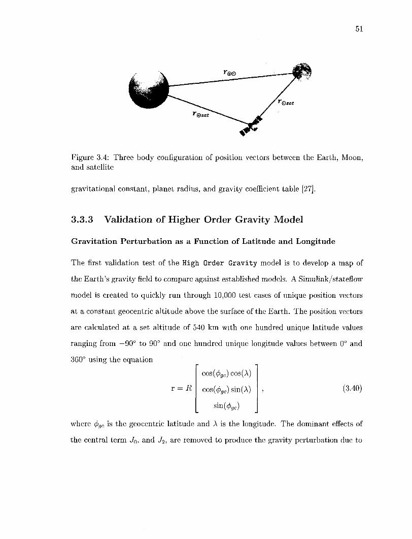
51

Figure 3.4: Three body configuration of position vectors between the Earth, Moon, and satellite

gravitational constant, planet radius, and gravity coefficient table [27].

3.3.3 Validation of Higher Order Gravity Model

Gravitat ion Per tu rba t ion as a Function of Lati tude and Longitude

The first validation test of the High Order Gravity model is to develop a map of

the Earth's gravity field to compare against established models. A Simulink/stateflow

model is created to quickly run through 10,000 test cases of unique position vectors

at a constant geocentric altitude above the surface of the Earth. The position vectors

are calculated at a set altitude of 540 km with one hundred unique latitude values

ranging from —90° to 90° and one hundred unique longitude values between 0° and

360° using the equation

r = R

cos 'gc ) cos(A)

cos(0gc) sin(A)

sin »gc)

(3.40)

where <pgc is the geocentric latitude and A is the longitude. The dominant effects of

the central term J0, and J2, are removed to produce the gravity perturbation due to

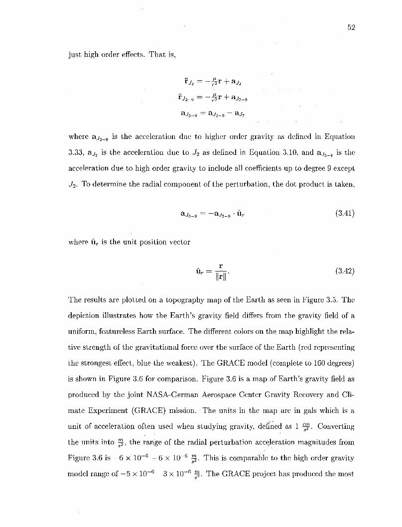
52

just high order effects. That is,

r J 2 - 9 = _ ^ 3 r + a ^ 2 - 9

aJ3-9 = a ^ 2 - 9 ~~ a ^ 2

where aj2_9 is the acceleration due to higher order gravity as defined in Equation

3.33, &j2 is the acceleration due to J^ as defined in Equation 3.10, and aj3_9 is the

acceleration due to high order gravity to include all coefficients up to degree 9 except

J2. To determine the radial component of the perturbation, the dot product is taken,

aj3_9 = -a j 3_9 • u r (3.41)

where u r is the unit position vector

Ur = |j^jj. (3.42)

The results are plotted on a topography map of the Earth as seen in Figure 3.5. The

depiction illustrates how the Earth's gravity field differs from the gravity field of a

uniform, featureless Earth surface. The different colors on the map highlight the rela

tive strength of the gravitational force over the surface of the Earth (red representing

the strongest effect, blue the weakest). The GRACE model (complete to 160 degrees)

is shown in Figure 3.6 for comparison. Figure 3.6 is a map of Earth's gravity field as

produced by the joint NASA-German Aerospace Center Gravity Recovery and Cli

mate Experiment (GRACE) mission. The units in the map are in gals which is a

unit of acceleration often used when studying gravity, defined as 1 ^ Converting

the units into *f, the range of the radial perturbation acceleration magnitudes from

Figure 3.6 is —6 x 10~6 — 6 x 10~6 I%. This is comparable to the high order gravity

model range of - 5 x 10"6 - 3 x 10"6 ^ . The GRACE project has produced the most

53

Longitude, X (deg)

Figure 3.5: Radial component of the gravitational perturbation, aj3_9 (^) , due to higher order gravity up to degree 9 excluding J<i with respect to latitude/longitude

update data on the Earth's gravity field. A comparison of Figure 3.5 and Figure 3.6

show enough similarities to establish a foundation to validate the implementation of

the High Order Gravity model. With the model validated, the effects of high order

gravity on satellite propagation is illustrated in the following section. Emphasis is

placed on the effects of higher order terms excluding J<2 to depict the importance of

applying high fidelity gravity models in accurate propagation tools.

Effects of High Order Gravitational Coefficients on Satellite Propagation

The potential generated by a non-spherical Earth causes periodic variations in all

the orbital elements. The largest perturbations, however, occur in the longitude of

ascending node and argument of perigee. The Earth's equatorial bulge introduces

a force component toward the equator which causes orbiting satellites to reach the

ascending node short of the crossing point for a spherical Earth. This westward

rotation is illustrated in Figure 3.7 which depicts a circular orbit with an altitude

of 300 km propagated over 10 periods with only higher order gravity perturbing the

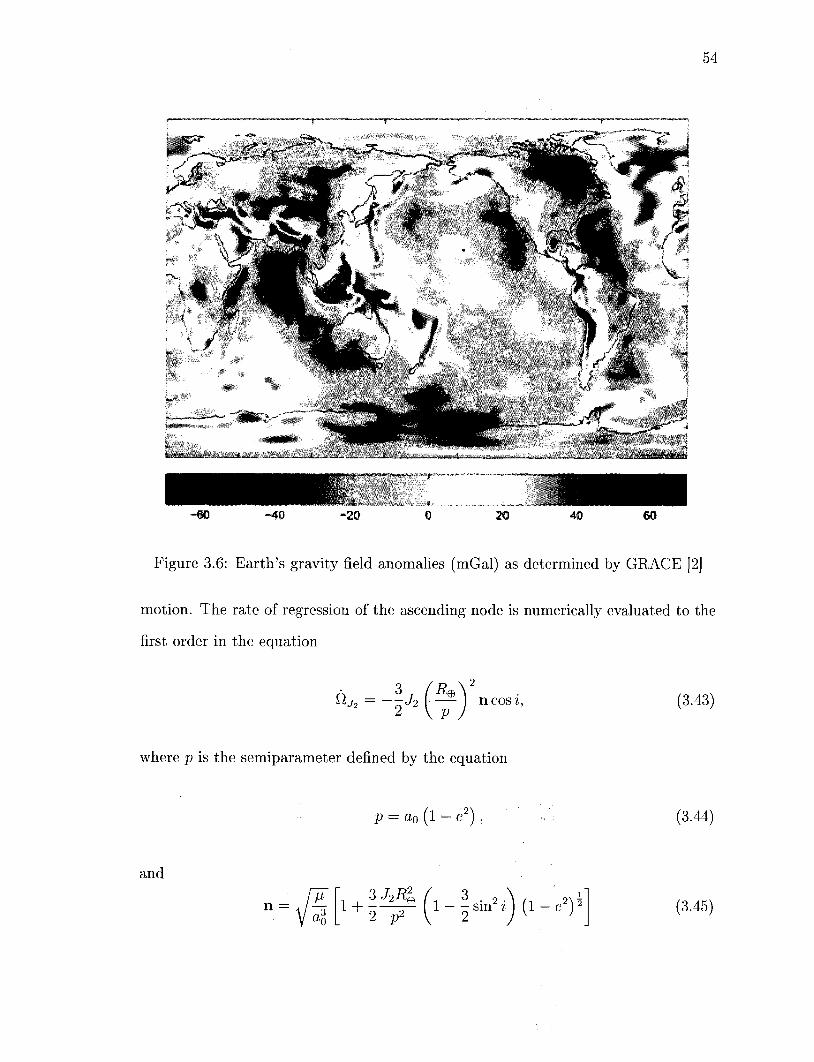
54

Figure 3.6: Earth's gravity field anomalies (mGal) as determined by GRACE [2]

motion. The rate of regression of the ascending node is numerically evaluated to the

first order in the equation

ttj2 = ~Jz ( —- ) ncosi, (3.43)

where p is the semiparameter defined by the equation

p = a0(l- e2) , (3.44)

and

n = W-7 1 + 3 JzRa

2 p2 l - - s i n 2 ; ) ( l ,2\i (3.45)

55

E

Nodal Regression Due to J2

_~^} Rotates Eastward

^ *.<% ** j&l ' , - **i%* / ^ SS * - .

Y(km)

Figure 3.7: The gravitational pull of the Earth's equatorial bulge causes the orbital plane of an eastbound satellite to regress westward

where n is the orbit mean motion with J2 correction. Further, it should be noted

that the node regresses for direct orbits and advances for retrograde orbits. There is

no nodal regression to first order for polar orbits. The secular motion of the perigee

occurs because the perturbed force is no longer proportional to the inverse square

radius and the orbit is consequently no longer a closed ellipse. The rate of change of

UJ is

-2~- 1N (3.46) CJJ2 = - J2 ( — ) n (5 cos2 i — l) . J2 4'

At the critical inclination of 63.43° or 116.57° the perturbation in the argument of

perigee is zero. Equations 3.43 and 3.46 highlight the relationship between inclination,

altitude and the rate of secular variation. For small values of inclination the cosine

56

function is driven to 1 increasing the rate. Likewise, for smaller values of altitude the

ratio of — becomes larger, also increasing the rate of perturbation. These trends are

highlighted in Figure 3.8 which plots the final position error due to J2-9 for circular

orbits with varying altitudes and inclinations propagated over one period. At an

altitude of 100 km, the deviation difference between an orbit with i = 0° and i = 90°

is 97 km after only one revolution. Further, at an inclination of 0° the deviation

difference between an orbit at an altitude of 100 km and 1000 km is 16 km.

Deviation in Final Position Over One Perioc! Dye t~a J „ . 2-9

Over Varying Inclinations and Attitudes with O - 0°

— a = 100 km • a = 200 km a = 300 km -a = 400 km a = 500 km a-800 km r

— s = 700 km — a = 800 km — a = 900 km l — a = 1000 km

"0 10 20 30 40 50 60 70 80 90 Inclination (deg)

Figure 3.8: Deviation in final position (km) due to J2-9 for circular orbits with varying altitudes and inclinations propagated over one period

Even with the dominant J2 coefficient removed, the higher order gravity coeffi

cients play a role in perturbing satellite motion. To illustrate this affect, the High

Order Gravity model is used in conjunction with an Encke Nystrom propagator to

test over 600 unique orbits. Each orbit has a distinct initial conic position and ve

locity calculated over varying inclinations and right ascension of ascending nodes.

All cases are propagated over one Keplerian orbit. The perturbation error between

the high order gravity model, J2-9, and the lower order gravity coefficient models is

computed by taking the magnitude difference in the initial and final position vectors

I H U

120 E

J 100 "re '> a> Q !

(A

£ 60

40

on

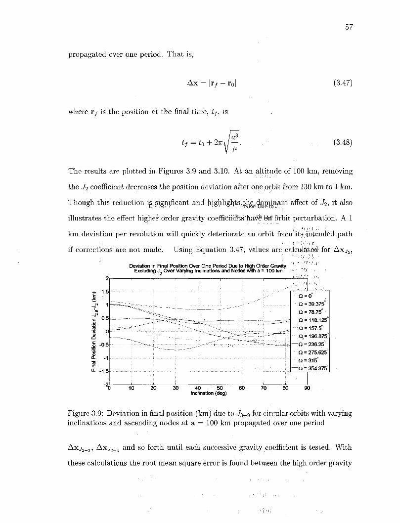
57

propagated over one period. That is,

Ax = I17 - r0| (3.47)

where 17 is the position at the final time, tf, is

tf = to + 27T4 (3.48)

The results are plotted in Figures 3.9 and 3.10. At an altitude of 100 km, removing

the J2 coefficient decreases the position deviation after one orbit from 130 km to 1 km.

Though this reduction is.significant and highlightsr)the dominant affect of J2, it also

illustrates the effect higher order gravity coefficieirts:'na# 8if Qrbit perturbation. A 1

km deviation per revolution will quickly deteriorate an orbit from its •intended path

if corrections are not made. Using Equation 3.47, values are calculated' for Axj2,

Deviation in Final Position Over One Period Due to High Order Gravity ' _ ' '' Excluding J Over Varying Inclinations and Nodes with a = 100 km r> •

40 50 Inclination (deg)

Figure 3.9: Deviation in final position (km) due to J^-g for circular orbits with varying inclinations and ascending nodes at a = 100 km propagated over one period

Axj2_3, A x j 2 4 and so forth until each successive gravity coefficient is tested. With

these calculations the root mean square error is found between the high order gravity

58

Deviation in Final Position Over One Period Due to High Order Gravity Excluding J . Over Varying Nodes and Inclinations with a = 100 km

150 200 Q(deg)

Figure 3.10: Deviation in final position (km) due to J3_g for circular orbits with varying ascending nodes and inclinations at a = 100 km propagated over one period

case, Axj2_9 and all the other gravity coefficient cases. For instance, comparing J2-9

and J2, one finds that

i2M5(Axj2_9 ,Ax j 2) 2 ^ i = l \XJ2-9,i XJ2,i)

n (3.49)

where n is the number of elements in the vector Ax.

The values produced in this case are compared to those produced in the NASA

report, The Gravitational Acceleration Equations [41]. The parameters are 630 test

cases with inclinations varying from 0°to 90° and the right ascension of ascending

node varying from 0° to 360°. The results are given in Table 3.1.

In comparing the High Order Gravity model output with the NASA legacy data,

two values were of interest: the "Truth Comparison", and the "Max Error". The

"Truth Comparison" columns in the table represent how each gravitational model

is compared against the 'truth', in this case the high order gravity model to the

9th order, J2~9- The 9th order is selected as the truth since it is the highest order

available at the time. Against itself, the J2_g model has no error, thus the results

59

Model Order

9 8 7 4 2

J2 only

NASA Model[41] RMS Error

82 83 129 273 538 789

Truth Comparison

0 1

47 191 456 707

Max Error

0 49 53 565 1130 1810

High Order Gravity Model RMS Error

0 40 101 233 444 701

Truth Comparison

0 40 101 233 444 701

Max Error

0 103 297 678 1167 1720

Table 3.1: Comparison of NASA and High Order Gravity model prediction position deviation

seen in the first row. The NASA model 'truth' values are smaller or very similar

to the High Order Gravity model values for all orders, with the largest discrepancy

between the 7th order models for the two, with a difference of only 54. Comparing the

maximum error between the two models yields a greater error for all the high order

cases produced by the High Order Gravity model, except J2 only. The information

between the two models is similar enough to further validate the accuracy of the high

order gravity model.

3.3.4 Model Configuration

As with all the perturbations modeled in this research, the High Order Gravity

model can be turned "on" or "off" based upon a user specified flag, fHOG, in the

initialization file. The default value '1 ' , turns the HOG model on, thus decomposing

the model into harmonics using Legendre polynomials. The value '0' for fHOG results

in the computation of the low terms J2 and J^JZJA, if a low fidelity model is required.

The specific gravity coefficients used by the modeldepend upon the 'degree' spec

ified by the user and the order of interest. See Table 3.2 for the effect of setting

different values for these parameters.

The gravity model is designed as a general model that can be applied to any

planetary body. For this reason the model must be initialized with values specific to

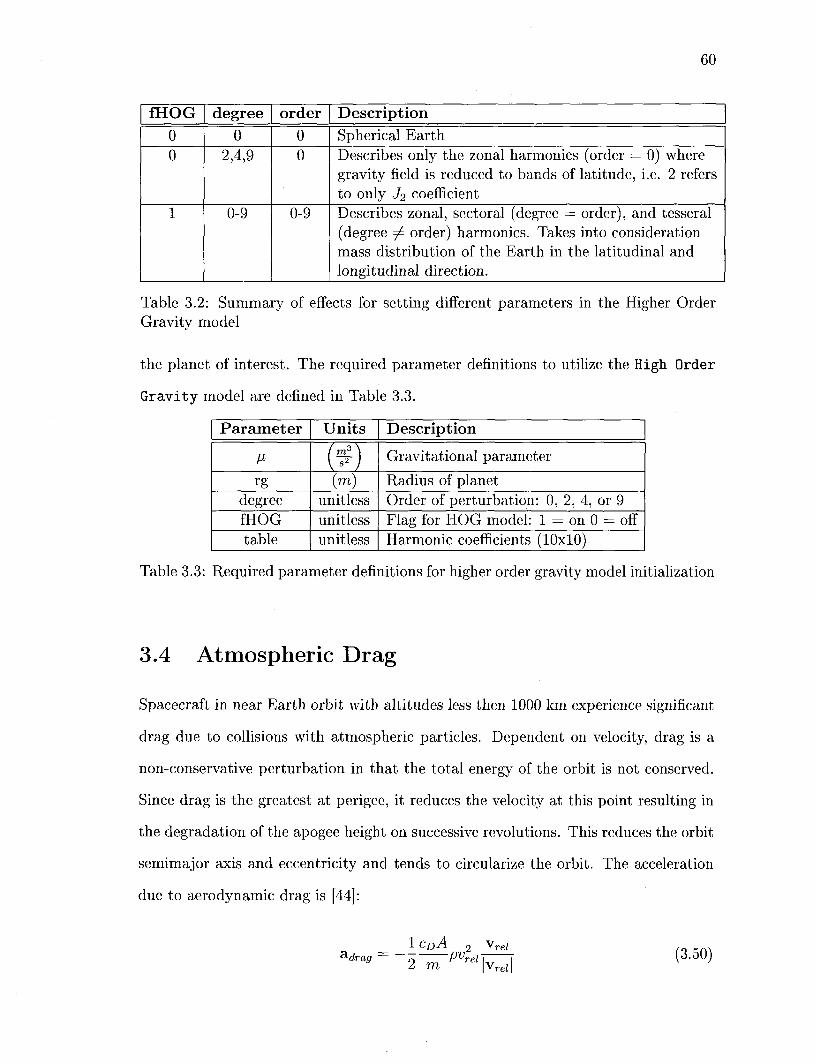
60

fHOG 0 0

1

degree 0

2,4,9

0-9

order 0 0

0-9

Description Spherical Earth Describes only the zonal harmonics (order = 0) where gravity field is reduced to bands of latitude, i.e. 2 refers to only Ji coefficient Describes zonal, sectoral (degree = order), and tesseral (degree ^ order) harmonics. Takes into consideration mass distribution of the Earth in the latitudinal and longitudinal direction.

Table 3.2: Summary of effects for setting different parameters in the Higher Order Gravity model

the planet of interest. The required parameter definitions to utilize the High Order

Gravity model are defined in Table 3.3.

Parameter

V r g

degree fHOG table

Units

( * ) (m)

unitless unitless unitless

Description

Gravitational parameter

Radius of planet Order of perturbation: 0, 2, 4, or 9 Flag for HOG model: 1 = on 0 = off Harmonic coefficients (10x10)

Table 3.3: Required parameter definitions for higher order gravity model initialization

3.4 Atmospheric Drag

Spacecraft in near Earth orbit with altitudes less then 1000 km experience significant

drag due to collisions with atmospheric particles. Dependent on velocity, drag is a

non-conservative perturbation in that the total energy of the orbit is not conserved.

Since drag is the greatest at perigee, it reduces the velocity at this point resulting in

the degradation of the apogee height on successive revolutions. This reduces the orbit

semimajor axis and eccentricity and tends to circularize the orbit. The acceleration

due to aerodynamic drag is [44]:

adi rag

ICDA

2 m -Pvrel]

Wrell (3.50)

61

The coefficient of drag, CD, is a dimensionless quantity which reflects the vehicle's

susceptibility to drag forces. Depending on the geometric form of the vehicle, the

coefficient is a difficult value to estimate. The mass, m, is assumed to be constant.

The cross-sectional area, A, normal to the velocity vector is difficult to accurately

compute due to the changing orientation of the vehicle. For this reason the area is

also approximated. Since Earth's atmosphere has a mean motion due to the Earth's

rotation, the velocity in the drag calculation must be relative to the atmosphere.

For simplicity, the program assumes no atmospheric rotation. The most challenging

parameter to calculate is the atmospheric density, p, which indicates how dense the

atmosphere is at a specific altitude.

The density distribution of a homogeneous, ideal gas with an altitude h is deter

mined by the ideal gas law [34]

> - & < -

and by the equation of hydrostatic balance,

Ap = -pgAh (3.52)

where p is the gas pressure. In the preceding equations, M is the mean molecular mass

of all atmospheric constituents, g is the acceleration due to gravity, R is the universal

gas constant, and T is the absolute temperature measured in Kelvins. Substituting p

from Equation 3.51 into Equation 3.52 and integrating Equation 3.52 from an initial

altitude h0 to a final altitude, h,

T0M ( [hgM \ P = P0TM-o

eXP{-JhoRTdh) (3-53)

the formula for atmospheric pressure and density is determined. In general, g, M,

and T are functions of altitude and time. The most challenging aspect in modeling

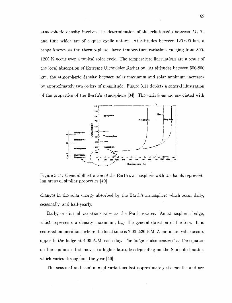
62

atmospheric density involves the determination of the relationship between M, T,

and time which are of a quasi-cyclic nature. At altitudes between 120-600 km, a

range known as the thermosphere, large temperature variations ranging from 800-

1200 K occur over a typical solar cycle. The temperature fluctuations are a result of

the local absorption of Extreme Ultraviolet Radiation. At altitudes between 500-800

km, the atmospheric density between solar maximum and solar minimum increases

by approximately two orders of magnitude. Figure 3.11 depicts a general illustration

of the properties of the Earth's atmosphere [34]. The variations are associated with

5000

900

800:

796

4- Exospitere

NighMi^e

Messs

DiytMa

I l l l l l n l l i l l U TOO 800 90® 1000 1100 1200

Tomperatare (K)

Figure 3.11: General illustration of the Earth's atmosphere with the bands representing areas of similar properties [49]

changes in the solar energy absorbed by the Earth's atmosphere which occur daily,

seasonally, and half-yearly.

Daily, or diurnal variations arise as the Earth rotates. An atmospheric bulge,

which represents a density maximum, lags the general direction of the Sun. It is

centered on meridians where the local time is 2:00-2:30 P.M. A minimum value occurs

opposite the bulge at 4:00 A.M. each day. The bulge is also centered at the equator

on the equinoxes but moves to higher latitudes depending on the Sun's declination

which varies throughout the year [49].

The seasonal and semi-annual variations last approximately six months and are

63

related to the varying distance of the Earth from the Sun as well as the Sun's decli

nation. Density variations are also related to the 11 year solar cycle which strongly

varies the amount of solar radiation that reaches the Earth.

For the calculation of Atmospheric Drag, a simplified static model of the atmo

sphere that only considers the altitude profile is employed. The model assumes the

entire atmosphere is isothermal and the density of the atmosphere decays exponen

tially with increasing altitude. Thus, from Equation 3.53, assuming T = T0 = const

and M = MQ = const, the density is calculated as

p = p0exp( j ~ ) , : ,. (3.54)

where po is the sea-level density, equal to 1.225 km/m3, and H — RT0/ (gMQ) = const

is the reciprocal of the atmospheric scale height set to 8.434 x 103 m [40]. Though

this model approximates much of the atmosphere, its simplifying assumptions induce

a large uncertainty in the accuracy of the model.

3.5 Solar Radiation

Solar radiation pressure is a result of the impact of light photons emitted from the

Sun on a vehicle's surface. Like drag, it is a non-conservative perturbation, but it has

a more pronounced effect at higher orbits and during interplanetary missions. Solar

radiation pressure is different from aerodynamic drag in that the force produced is in

the antisolar direction, rather than always opposite the spacecraft's velocity vector.

For this reason the effects of solar radiation may average close to zero for orbits

which experience periods of solar occupation by the Earth [24]. The acceleration due

to solar radiation is calculated by the equation

PSRCRA® 1 Sat® / 0 r r - \

&SR =. 1 r, ••' • » (3.55) m Irsat© I

64

where PSR, is the solar pressure per unit area, or the change in momentum defined as

PSR = 4.57 x 1CT 6 ^ . (3.56) m2

The variable CR is the reflectivity and can have a value between 0.0 and 2.0, indicat

ing how the vehicle reflects incoming radiation. A value of 0.0 means the object is

translucent to radiation, and thus no force is transmitted. A value of 1.0 indicates

all the radiation is absorbed and all the force is transmitted. Finally, a value of 2.0

means all the radiation is reflected and twice the force is transmitted [49]. A® is the

area of the spacecraft exposed to the Sun. Determining both CR and A® is difficult

as the vehicle is often changing altitude. For this reason, an average value is selected

for both based on the possible orientations of the vehicle throughout the flight. The

variable m is the mass of the vehicle and, depending on the mission, may change dras

tically over time. For simplicity purposes the mass is assumed constant. However, if

a thrust model were added the mass would be computed as an additional state. The

symbol rsai€) denotes the position vector from the vehicle to the Sun; because this

vector always points away from the sun, a unit vector yields the appropriate sign. The

SPICE ephemeris program is used to calculate the position of the Sun with respect

to the vehicle.

Solar radiation pressure does not act on a spacecraft during periods of solar oc

cupation by the Earth or other bodies. As a result a program such as Shadow, as

defined in Vallado [49], can be utilized to determine whether or not the spacecraft is

in complete sunlight, penumbra, or umbra.

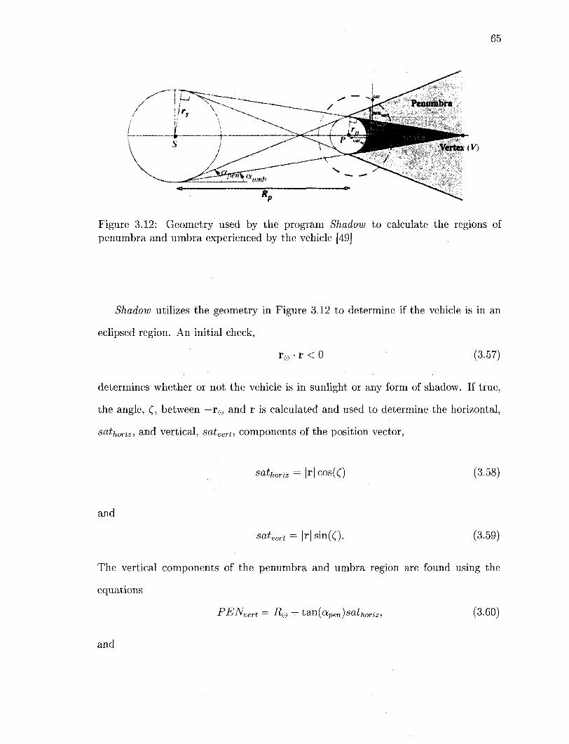
65

Figure 3.12: Geometry used by the program Shadow to calculate the regions of penumbra and umbra experienced by the vehicle [49]

Shadow utilizes the geometry in Figure 3.12 to determine if the vehicle is in an

eclipsed region. An initial check,

r 0 • r < 0 (3.57)

determines whether or not the vehicle is in sunlight or any form of shadow. If true,

the angle, (, between —r0 and r is calculated and used to determine the horizontal,

sathorizi a n d vertical, satvert, components of the position vector,

sathoriz = |r| cos(C) (3.58)

and

satvert = |r| sin(C). (3.59)

The vertical components of the penumbra and umbra region are found using the

equations

PENvert = R& + tsai(apen)sathoriz, (3.60)

and

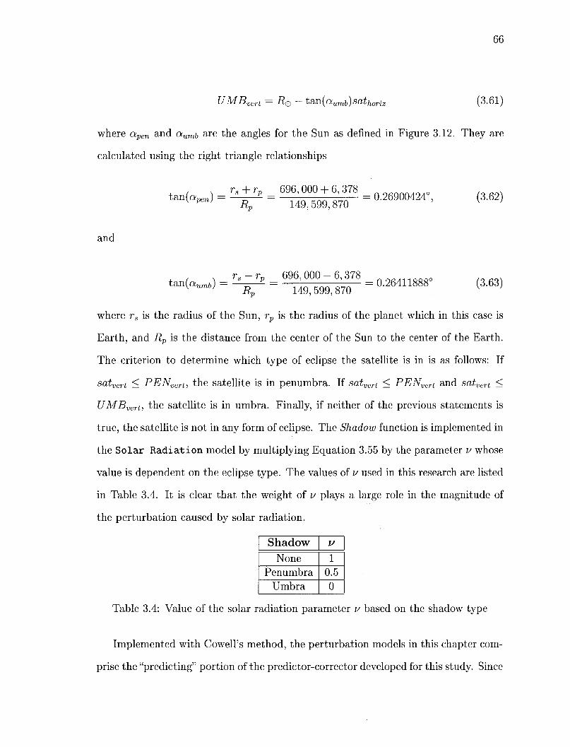
66

UMBvert = R@- tan(aumb)satho (3.61)

where apen and aumb are the angles for the Sun as defined in Figure 3.12. They are

calculated using the right triangle relationships

tan(aperi) rs + rp

Rp

696,000 + 6, 378 149,599,870

= 0.26900424°, (3.62)

and

tan(aum6) = Rr,

696, 000 - 6,378 149, 599,870

= 0.26411888° (3.63)

where rs is the radius of the Sun, rp is the radius of the planet which in this case is

Earth, and Rp is the distance from the center of the Sun to the center of the Earth.

The criterion to determine which type of eclipse the satellite is in is as follows: If

satvert < PENvert, the satellite is in penumbra. If satvert < PENvert and satvert <

UMBvert, the satellite is in umbra. Finally, if neither of the previous statements is

true, the satellite is not in any form of eclipse. The Shadow function is implemented in

the Solar Radiation model by multiplying Equation 3.55 by the parameter v whose

value is dependent on the eclipse type. The values of v used in this research are listed

in Table 3.4. It is clear that the weight of v plays a large role in the magnitude of

the perturbation caused by solar radiation.

Shadow None

Penumbra Umbra

V

1 0.5 0

Table 3.4: Value of the solar radiation parameter v based on the shadow type

Implemented with Cowell's method, the perturbation models in this chapter com

prise the "predicting" portion of the predictor-corrector developed for this study. Since

67

the final propagated states will not always match up with the desired values, a means

of correction to the initial states is implemented. The following chapter develops the

corresponding "correcting" part of the process.

Chapter 4

State Transition Matrix

The following chapter describes the error state transition matrix that forms the basis

for the "corrector" used in the predictor-corrector algorithm for this thesis. The state

transition matrix linearizes the trajectory determination problem to further refine

the initial velocity guess to produce a final high fidelity trajectory. The derivation

of the partial derivatives of the perturbations discussed in the previous chapter are

also considered. The accuracy of the matrix is demonstrated over varying times of

flight and initial perturbation percentages to demonstrate the linear sensitivity region.

Finally, the application of the matrix in a shooting method technique is demonstrated.

The derivative of the state transition matrix begins by assuming the existence of

two close trajectories. Of the two trajectories, only one is known. To determine the

unknown trajectory the difference between the two trajectories is computed. If the

two trajectories are X and Y, the initial conditions and derivatives of the states are

defined as [49]

X ( t 0 ) = X 0 and X = / (X) ,

Y ( * 0 ) = Y o and Y = / ( Y )

where / denotes a function of the state. If the difference between the two trajectories

68

69

is 5x, then

Y = X + 5x. (4.2)

Substituting Equation 4.2 into Equation 4.1 results in

Y = / ( X + 5x). (4.3)

Since / ( X + #x) is nonlinear, the function is expanded in a Taylor series about X,

(5x = Y - X),

Y = / (X) + <9/(xK , ^r(x -<5x + -<5x2 + ... (4.4) ax 2!dX2

where / (X) is a time varying square matrix. The time derivative of Equation 4.2 is

taken and substituted into the left-hand side of Equation 4.4

X + S± = /(X) + ft/ d / ( X h df(X)

a x 2!<9X2 5x2 + (4.5)

which using Equation 4.1 is reduced to the equation

5x = JL y £x + u = G<5x + u. oX

(4.6)

Here u represents the neglected higher order terms and G is a matrix of partial

derivatives known as the Jacobian matrix which represents the linearized dynamics.

Its solution is the time-varying difference between the two neighboring trajectories.

A relationship for the G matrix is found by assuming a solution to Equation 4.6

of the form

5x = $(t,t0)5x0 (4-7)

which is also written as

Sr

5v = $(Mo)

<Sr0

5v0

(4.8)

70

For these equations u = 0 and <& (t, t0) is the state transition matrix which relates an

initial set of perturbed state vectors to a final set of perturbed state vectors over a

given period of time [48] [5]. The components of the matrix are

$(Mo) =

where

$n =

dr <9ro

J2X dr0

dr <9r0_

dr dv0

dv dv0

$11 $12

$ 2 1 $22

dx dx dx dxo dyo dzo

9y dy dy dxo dyo dz0

dz dz dz 9xo dy0 dzo

(4.9)

(4.10)

The state is numerically integrated using the matrix differential equation which is

found by taking the derivative of Equation 4.7,

6± = <Mx0 + $<5x0 (4.11)

where <5x0 = 0. Substituting Equation 4.6 into Equation 4.11 produces

G<Sx = $(5x0. (4.12)

Substituting the right side of Equation 4.7 back into Equation 4.12 produces

G $ (t, t0) 5x0 = $ (*, h) 5x0 (4.13)

which reduces to the first-order differential equation

6(Mo) = G$(Mo), (4.14)

71

with the initial condition

$(Mo) = Iex6- (4.15)

Note the dynamic coefficient matrix consists of nonlinear, time-varying terms G\ = ^

G = (4.16)

and G2 = f:

03x3 13x3

G\ (?2

The following describes the development of the partials for each individual perturba

tion required by G\ and G2 in Equation 4.16.

4.1 N-Body Partials

The most basic state transition matrix consists of partials calculated from the two-

body conic motion derived from Equation 2.10,

r(Bsat ®sat

(4.17)

As previously mentioned, an analytic solution exists for conic motion. One derivation

of the analytic Keplerian matrix is found in Reference [45]. The simplest partials to

add to the conic state transition matrix are those resulting from three body acceler

ation. From Equation 3.1 one derives that

r®sat — A% ^0 ^o

~r Q l-satQ —3 *©©• ^sat

$sat ' r 3 satO ' ©0

Thus, |^ = fn(r,t). The partials on the diagonal have the form

dfi /% 3/%r

dri + + Qsat Qsat Qsat

(4.18)

(4.19)

72

All other sub-components of the matrix are defined as

Ul J ' (Bsat ' Qsat (4.20)

where i and j refer to any vector sub-components x, y, or z. To add in a fourth

body to the state transition matrix, such as the Sun, the last two terms of Equation

4.19 and the last term in Equation 4.20 are repeated with fj, and the position vectors

updated so they are with respect to the fourth body. Thus, the updated Equations

4.19-4.20 are

dri

^ 9

^sat 1 ®sat

M© , 3 M 0

Qsat,i + Qsat Qsat

/%

©sat

3fI®r<$ISat,i (4.21) ®sat

Uri _ {->l1®r®sat,if®sat,j ^^QrQsat,ifQsat,j ^^®r®sat,ir®sat,j . , • , . „ 9 \ fir. ~ r5

+ r 5 +

r 5 i 3 T l \^-zz) Ul 3 '(Bsat 'Qsat ' ®sat

where the subscript © refers to the Sun. The equations can be rewritten in a gener

alized form to include n-bodies:

dri

dri

n

i=3

n ,

J'=3 V

.( 1 , ' V r3

\ jsat

'J'rjsat,iTjsat,j

jsat

Q r 2 jsat,i

jsat

) • •

J V «

(4.23)

(4.24)

Since for acceleration due to n-bodies, r is only a function of position, the dynamic

coefficient matrix reduces to:

0 I

Gi 0 G = (4.25)

The state transition matrix is propagated forward in time using the variable step

differential equation solvers discussed in Section 2.8.5. For each time step the SPICE

73

ephemeris program calculates the updated position vector of the Moon and or Sun

as needed in Equations 4.19-4.20.

4.2 Gravity Potential Partials

The state transition matrix can be updated to include more complex perturbations

such as higher order gravity, drag, and solar radiation. Like the three-body equations

of motion, the equations due to the non-spherical Earth depend only on the satellite's

position, |^ = fn(r,t), and thus no partials are taken with respect to velocity. The

following derivation is based on Long's [25] calculations of the partials of the potential

function as seen in Equation 3.18. To maintain conformity with Long's development,

the potential function variable </> is replaced by U. Thus, the acceleration due to

high order gravity is the gradient of the potential function, aj2_9 = ^ , which is

transformed into spherical coordinates for simplicity. That is,

a J 2 - 9 — dU dUdr OUdX dU d<\>

dr dr dr d\ dr d(f> dr (4.26)

The partial of a j 2 9 with respect to r is found by differentiating Equation 4.26. Specif

ically, — J . (§U.\ dr , d_ (8U\ d± , d__ ( dU\ dX

dr V dr ) dr "t" dr \ d<f> J 3r "'" dr \ d\ J 9r

daJ2-dr

_L.dU_<Pr_ , d]l§P± , dUd2\ ~T~ dr 9r2 "r dd> 9r2 "•" dX dr2 '

(4.27)

where the partial derivatives of | f, ^ , and | ^ with respect to r are obtained using

the following matrix

r) dr

dU dr

dU 8<j>

dU dX

—

d2 U dr2

d2U d<f>dr

d2U dXdr

d2U drd<f>

d2U d24>

d2U dXdtp

d2U drdX

d2U 84>dX

d2U dX2

dr 9r

d± dr

dX 9r

(4.28)

74

The second partial derivatives of the potential are

x

0 = ^ E ~ 2 ( ^ ) " ( « + 2)(n + l)

V " (C™ cos m\ + S™ sin mA) P™ (sin <f>),

a2u _ a2u = -%En=2(^y(ri + l) drd<j> d(j>dr

x Em=o (Cn c o s mX + S™ s i n mX) \pn+1 (sin 0) - m tan </>P™ (sin <

a2u _ a2u drd\ d\dr

Ml

r3 Z_/n=2 I r ) fn + 11

x Em=o m (s™ cos mA — C™ sin mA) P™ (sin </>),

(4.29)

(4.30)

(4.31)

W = r E^=2 ( ^ ) E™=o (<3T COS m A + S? s i n™*) [tan 0P-+ 1 (sm,

+ [m2 sec2 4> — m tan2 0 — n(n + 1)] P™ (sin </>)],

a2(j _ s:

d4>8\ axk = ? £ £ * ( ^ ) n E ^ = o ^ ( ^ m c o s m A - C - s i n m A )

x [P™+1 (sin 0) - m tan </>P™ (sin 0)],

and

(4.32)

(4.33)

d2U dX2 = -Vj2[ — ) Yl ™2 (Cn c o s m X + Sn s inmX) P™ (sin(j)). (4.34)

n=2 ^ ' m=0

The partial derivatives of r, 0, and A with respect to r, where r = [ Tx rv rz] a r e

d(f)

dr

dr T

r1

dr r '

1

Vrx + ry

rzrT drz

r2 dr

and dX dr,. drr

dr (r2 + r2) — r. dr dr

(4.35)

(4.36)

(4.37)

75

The required second partial derivatives of r, </>, and A in Equation 4.27 are found by

differentiating Equations 4.35-4.37 with respect to r. That is,

d2r dr2 I - rr (4.38)

and

& l+'l)

\ dr) "fr Tx \~dt) + Tj \ dr )

l^/rl+rl m+rj % r r T (4.39)

d2X dr2 ( r 2 + r 2 )

0

or J V or + (rl + rl)

0 - 1 0

1 0 0

0 0 0

where ^ Or

drv

(4.40)

1,0,0) , ^ = (0,1,0), and ^ = (0,0,1). To reduce the analyti

cal computations necessary for taking the partial derivatives of a high order gravity

model, the partials for only J2, J3 , and J4 are considered.

When taking the partials of Equation 3.10, consider first the partials with respect

to the x and y components of both the acceleration and position vectors. The partial

on the diagonal is

?2 „,2^2 daj2^ _ 3 J 2 ^ K , 15J2/x-R^rf 15J2fiR2erj _ 105J2^R2

erfr2z

dn 2r5 2r7 2r7 2r9

and the partial on the off diagonals is

daj2:i _ 15J2/ii?|nO 105J2nRlrirjr2z

* r J-dr-i 2r7 2r9 (4.42)

76

The partial of the z component of the acceleration vector on the diagonal is

daj2tZ _ VJ2tiRl 45J^R2er

2z 105J2//^r,4

drz 2r5 r7 2r9 [ ' '

and the partial on the off diagonals for the z component is

daj^z _ 45J2fiRl)rirz _ 105J2//i4nr1 dr, ~ 2r7 2r9 (4.44)

Similar equations exist for the partials of the acceleration due to J3 and J4 (Equa

tions 3.12-3.13). Again, considering the partials just with respect to the x and y

components, the diagonal term is

daj3,i = l5J3nR%rz 1 0 5 J 3 ^ r t2 r 2 35J3//i?|rf 315J3^-R|rfrf

On ~ 2r7 2r9 2r9 2 r n ' [ }

and daj4ii _ 1 5 J 4 M J R | 105.7 4 ;^r f . 1 0 5 J 4 / ^ r f 945J4/xJR4j?fr2

dn 8r7 ' 8r9 ' 4r9

315J4/ii^rf 3465J4/ii^rfr2 8 r i i 1 8 r i 3

The off diagonal equations are

daj3^ _ 105J3fiR%rirjrz 3 1 5 J ^ - R ^ r ^

drj 2r9 2 r n

4 r i i

i^J,

(4.46)

(4.47)

and

^Qj4,i _ 105J4/^Rer*rJ _ ^J^R^rjTjrl 3465J4/ii?er 'rJr^ • / • /4 4OA a r . - 8 r9 4 r i i + 8 r i3 ^ ^ i 4 ' 4 ^

The partial of the z component of the J3 and J4 acceleration vectors on the diagonal

are daj3,z 75J3nRlrz 1 7 5 J 3 ^ | r f 3 1 5 J 3 / ^ r f

dr2 2r7 + r9 2 r n ' { '

77

and

da J\,z 75J4/xfli 1575J4//i?ir2 4725J^Rir4z 3465J4fiR%r\

dr. 8r7 8r9 8r 11 8r13 (4.50)

Further, the partials on the off diagonal for the z component of the J3 and J4 accel

eration vectors are

3 ^ ~4 dcLj^z _ 105J3fiRs9rir2

z 315J3/ii?|rjr| 15J3/xi^r. dr; 2r 11 2r7 (4.51)

and daj4:Z 525J4//i?^rjrz 1575J4/ii?^rjr^ 3465J4//.Rj|rjr ? 4 „ . . r 5

z

dr. 8r9 4r 11 8 r 1 3

9 a Again, because —^H4- = fn(r,t), the dynamics coefficient matrix is

(4.52)

G = 0 I

Gi 0 (4.53)

where Gi is rewritten as

Gi =

9 a j , drx

daj2,y drx

+ 9 a j .

9 r x + 9 a J4,x

drx

da J2, drx

+ +

da J3<y drx

drx

+ da

drx

+ da J4,z

drx

da J2,:

J4,!/ aaJ2iy

dry

da.,

, dajs<x

drv

dr„ + da J3'V

drv +

daj4,x

dry

9aj4,y

drv

da •>2'z

drv + da •*3v

drv ~T~ drv

da J2<x

drz

drz

daj2,: drz

da J3 ,x daj.

drz drz

daJ2,v 1 daJ3,v drz

9aj3,z

drz

+ da Jj,y

drz

+ da J^,z

drz

.54)

4.3 Atmospheric Drag Partials

From Equation 3.50 it is clear that to incorporate drag into the state transition

matrix the partials due to due both position and velocity are required. The partial

78

with respect to the position vector is

da, drag,i GpAp^Tj , 2 . 2 , 2\~h I \Tx "*" Ty + Tz) ^ ^ 9 _ ^ - " ^ ( r - + r

S / + rZ ) eXP 3rj H

The partial with respect to velocity on the diagonal is

{v'i + v\ + v2) Vi.

(4.55)

dVi

CpApp 2m [(*( v2

x + vl + vl) * +

(vl + vl+vl)*\ exp H

(4.56)

and the partial with respect to velocity on the off diagonal is

dadrag,i _ CpAp0

dvj 2m (vl + Vy+ vl) 2 ViVj exp (ri + rj + f^y-Ik

H . (4.57)

Since agrra9 = fn(r,v,t), the dynamics coefficient matrix is

G 0 I

G\ G2 (4.58)

Summarizing, the G\ sub-component of the dynamics coefficients matrix can be writ

ten as

G i

dad, lrag,x dadrag,x ®adrag,x drx

W>dvag,y drx

UQ'drag,z drx

dr„

dad '•rag,y dry

d®drag,. dr y

drz

^^drag,y drz

OQ'drag,z dr.

(4.59)

and similarly the G2 component can be written as

G,=

&adrag,x dvx

&Q'drag,y dvx

&Q'drag,z

UQ>drag,x OVy

^^•drag,y dVy

UQ'drag,z

UQ'drag,x dvz

&Q'drag,y dvz

&adrag,z 8vx 8Vy dvz

(4.60)

79

4.4 Accuracy of Error State Transition Matrix

In addition to the partials previously discussed, perturbation partials for solar radia

tion and higher order gravity can be added to the state transition matrix to ensure the

greatest accuracy. However, as additional terms are included in the matrix it becomes

computationally more costly to integrate. A motivating factor for the development of

the Cowell-STM predictor-corrector is the option of generating solutions efficiently.

Thus, finding the balance between accuracy and computation time is critical.

A number of state transition matrices are calculated with varying levels of fidelity.

The matrices tested are listed in Table 4.1. Each is put through two main tests to

STM Label 2-Body 3-Body 4-Body

4-BodyJ2

4-Body J2J3

4-Body ,/2Drag

Perturbations Included 2-Body (Earth) 3-Body (Earth and Moon) 4-Body (Earth, Moon, and Sun) 4-Body (Earth, Moon, and Sun), J2 gravity coefficient (Earth) 4-Body (Earth, Moon, and Sun), J2 and J3 gravity coefficients (Earth) 4-Body (Earth, Moon, and Sun), J2 gravity coefficient (Earth), and drag

Table 4.1: List of varying fidelity state transition matrices tested for selection purposes

determine the relative accuracy and sensitivity of the matrix. The first test varies the

transfer time for one set of initial states. Since the STM is numerically integrated,

longer propagation times will inherently accumulate more error. The test illustrates

the rate of the increasing error as well as compares the relative accuracy of each state

transition matrix.

The transfer time test consists of selecting initial states (r0, v0, t0) which remain

constant as the value for tf varies in small increments up to the total transfer time.

Using the initial states and transfer time, the Cowell propagator calculates the final

states using

X = /(X,*) (4.61)

80

with the initial condition,

X 0 =

thus,

r0

v0

*/ . X , = / Xdt.

to

(4.62)

(4.63)

Along with the dynamics coefficient matrix the state transition matrix is computed

as,

with the initial condition

${tt,to) = G$(tf,t0),

$0 = W

(4.64)

(4.65)

Next an initial perturbation of 0.01% involves adding to the radial component of the

position vector

rPert = r0 + 5r, (4.66)

where

ST = 0 . 0 0 1 ^ . ro

(4.67)

Using rpert as the initial position, the Cowell propagator calculates the final states

again using Equation 4.61 and Equation 4.63,

X •fpert

tf Xdt (4.68)

to

with the new initial condition,

X0 + SXQ, (4.69)

81

where £Xn = ST

0 . The difference between the two Cowell propagations is the

expected error in the final states due to the initial perturbation

AXcOTe«(t/, t0) — X/pert — X/. (4.70)

The expected error is also calculated using the state transition matrix

AXsTM{tf,t0) = $ 0

(4.71)

The magnitude difference between the Cowell and STM prediction is the error for

state transition matrix for that transfer time. That is,

Error = \AXcoweu(tf,to) - AXSTM(*/ ,2O) | • (4.72)

The second test varies the initial perturbation percentage for the same initial

state with a constant transfer time. Since the analytic state transition matrix is

derived from linear approximations along the Keplerian trajectory, the perturbations

must remain small. This characteristic is true for all state transition matrices. If the

deviations are too large the problem becomes nonlinear and the state transition matrix

cannot predict an accurate resultant error. By varying the initial perturbations, the

point at which the perturbations become too large for the matrix to accurately handle

is identified, illustrating the limitations of the STM. Furthermore, the test highlights

which matrices are least sensitive to varying perturbations.

The initial perturbation percentages range from 0.001% - 9%. The test is per

formed using the exact algorithm as the time test to determine the error in the

individual state transition matrices. Since this research focuses on both low Earth

orbit and translunar trajectories a general case from each category is selected for the

82

transfer time test and perturbation percentage test. The results are presented in the

following section.

4.4.1 Low Earth Orbit Transfer Test Results

The initial conditions for the low Earth orbit transfer case are listed in Table 4.2.

Parameter a e i

n U!

V

r0

v0

to

tf

Initial Orbit 100 km

0.1 0° 0° 0° 0°

Final Orbit 400 km

0.1 0° 0° 0°

180° [6.478 0 0] km

[0 8.226 0] km/s 0 sec

100-3200 sec

Table 4.2: Initial conditions for low Earth orbit state transition matrix time accuracy test

Figure 4.1 illustrates the orbit propagated over the complete 3,200 second transfer

time. During this propagation the individual perturbation magnitudes are recorded

and plotted in Figure 4.2. The acceleration of the non-conic Earth gravity remains

large throughout the trajectory due to the effect of J^ on equatorial orbits. As

expected, the acceleration due to the Earth's gravitational pull decreases and the

three-body effects of the Earth, Sun, and Moon increase as the vehicle moves towards

the apogee of its final orbit. Due to the large distance between the vehicle and the

Moon for the entirety of the transfer, the acceleration due to lunar gravity remains

small. At the perigee of the orbit drag plays a significant role, however it quickly

diminishes as the vehicle travels out of the Earth's dense atmosphere. Finally, solar

radiation remains small, on the magnitude of 10~u , and at one point drops to zero

as the satellite enters the Earth's shadow. Figure 4.2 highlights both dominating and

insignificant perturbations to the vehicle in low Earth orbit transfers. However it is

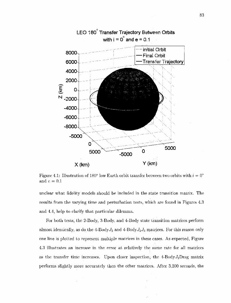
83

LEO 180 Transfer Trajectory Between Orbits with i = 0° and e = 0.1

— Initia —Final

Orbit Orbit

—Transfer Trajectory

5000

X(km)

Figure 4.1: Illustration of 180° low Earth orbit transfer between two orbits with i = 0° and e = 0.1

unclear what fidelity models should be included in the state transition matrix. The

results from the varying time and perturbation tests, which are found in Figures 4.3

and 4.4, help to clarify that particular dilemma.

For both tests, the 2-Body, 3-Body, and 4-Body state transition matrices perform

almost identically, as do the 4-BodyJ2 a n d 4-BodyJ2 J3 matrices. For this reason only

one line is plotted to represent multiple matrices in these cases. As expected, Figure

4.3 illustrates an increase in the error at relatively the same rate for all matrices

as the transfer time increases. Upon closer inspection, the 4-BodyJ2Drag matrix

performs slightly more accurately then the other matrices. After 3,200 seconds, the

84

Acceleration of Individual Perturbations for LEO Transfer with i = 0 and e = 0.1 10

10'

I 10"

v o 3

10

,-12;

10

10

-Non-Conic Earth Gravity -Non-Conic Lunar Gravity Three Body Motion

-Drag -Solar Pressure

10 20 30 Time (min)

40 50 60

Figure 4.2: Individual perturbation magnitudes for 180° low Earth orbit transfer between two orbits with i = 0° and e = 0.1

4-Body J2Drag matrix is 40 meters more accurate then any other matrix.

The perturbation test and Figure 4.4 illustrates that all the matrices are quite

sensitive to initial perturbations. A perturbation percentage of only 0.3% in the radial

direction of the position vector results in an error of 1,200 km after 3,200 seconds. As

the perturbation percentages increases the non-linearity of the drag model results in

the matrix producing the greatest error. Closer inspection reveals that to maintain an ; •:"'.'•• * ,;' . . • • . - . • • V i . v v o e i " '•'.•••

error under 12 km for a 3,200 second propagation, the, maximum deviation the STMs

can handle is 0.001%. A more detailed analysis again illustrates the accuracy of the

4-Body J2Drag matrix over the other matrices. At an hwtte^Jp&rturbation percentage

of 0.0018%, the 4-Body J2Drag matrix is 70 meters more1 'accurate then the 4-Body J2

or 4-Body J2J2 STMs and 80 meters more accurate then the n-body matrices (2-Body,

3-Body, 4-Body). '

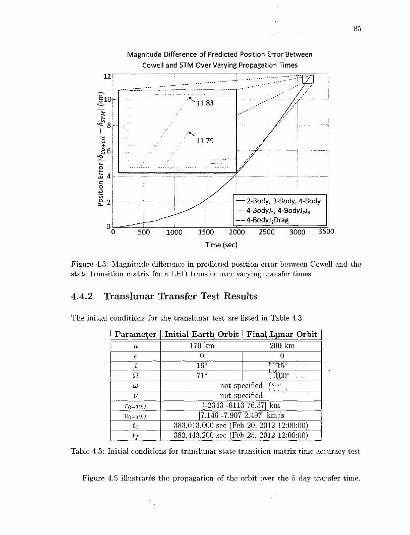
85

12

J10

<o 8

Magnitude Difference of Predicted Position Error Between Cowell and STM Over Varying Propagation Times

! _ ! -i-.I

V 11.83

• ' V

11.79

— 2-Body, 3-Body, 4-Body 4-Bodyi2s 4-BodyJ2J3

— 4-BodyJ2Drag

500 1000 1500 2000

Time (sec)

2500 3000 3500

Figure 4.3: Magnitude difference in predicted position error between Cowell and the state transition matrix for a LEO transfer over varying transfer times

4.4.2 Translunar Transfer Test Results

The initial conditions for the translunar test are listed in Table 4.3.

Parameter, a e i Q

L)

V

TO-TLI

VQ-TLI

to tf

Initial Earth Orbit 170 km

0 16° 71°

Fina} I^inar Orbit 200 km

0 N" ! i -5 0

;(4PD° ... .. not specified ;"''- not specified

[-2343 -6113 76.57] km [7.146 -7.907 2.497] km/s

383,013,000 sec (Feb 20, 2012 12:00:00) 383,443,200 sec (Feb 25, 2012 12:00:00)

Table 4.3: Initial conditions for translunar state transition matrix time accuracy test

Figure 4.5 illustrates the propagation of the orbit over the 5 day transfer time.

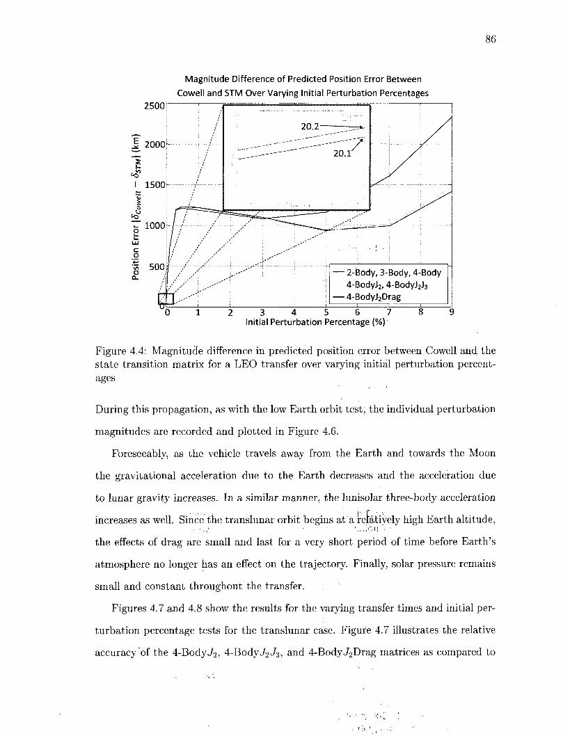
86

Magnitude Difference of Predicted Position Error Between

Cowell and STM Over Varying Initial Perturbation Percentages

• 0 1 = - i ! I I M ' I I I ' I

0 1 2 3 4 5 6 7 8 9 Initial Perturbation Percentage (%)

Figure 4.4: Magnitude difference in predicted position error between Cowell and the state transition matrix for a LEO transfer over varying initial perturbation percentages

During this propagation, as with the low Earth orbit test, the individual perturbation

magnitudes are recorded and plotted in Figure 4.6.

Foreseeably, as the vehicle travels away from the Earth and towards the Moon

the gravitational acceleration due to the Earth decreases and the acceleration due

to lunar gravity increases. In a similar manner, the lunisolar three-body acceleration

increases as well. Since the translunar orbit begins at'a •relatively high Earth altitude, • . „ ' • • . " \...',QD '•

the effects of drag are small and last for a very short period of time before Earth's

atmosphere no longer has an effect on the trajectory. Finally, solar pressure remains

small and constant throughout the transfer.

Figures 4.7 and 4.8 show the results for the varying transfer times and initial per

turbation percentage tests for the translunar case. Figure 4.7 illustrates the relative

accuracy of the 4-BodyJ2, 4-BodyJ2J3, and 4-BodyJ2Drag matrices as compared to

87

Translunar Transfer Trajectory With Earth Conditions i = 16 Q = 71 and Lunar Conditions i = 15° U = 100°

150F

100

50

E

U 1 1 1 4 1 1 i i r

—Transfer Trajectory —Moon Trajactory

1 -

: ^ ^ \

^ _ _ _ - _ _ _ _ _ ^ — ^ ;

1 - i i i i \ i i i i-r i -

-50-

-100

-150 -50 0 50 100 150 200 250 300 350 400

X (kkm)

Figure 4.5: Illustration of a 5 day translunar transfer with conditions % ne = 71° and iQ = 15° Q 0 = 100°

= 16°

the n-body matrices for majority of the transfer times. However, as the trajectory

nears the Moon all the matrices become highly inaccurate when compared to the

propagated Cowell states. This is because none of the matrices model the gravita

tional pull of the Moon, which as illustrated in Figure 4.6, becomes a dominating

force at the end of the transfer period.

The results highlighted in Figure 4.8 show a similar trend as those for the LEO

case in Figure 4.4. All of the matrices are extremely sensitive to initial perturbations.

Depending on the matrix, an initial perturbation of only 1% in the position vector

can lead to an error of 500,000 km over the 5 day translunar transfer. Again, the

higher fidelity matrices, such as those including additional gravity coefficients and

drag produce the worse results for the larger perturbation percentages. However,

closer analysis reveals that at perturbation percentages less than 0.009%, the same

models perform much more accurately (under 1000 km error).

After analyzing the cumulative results of the varying time and initial perturba-

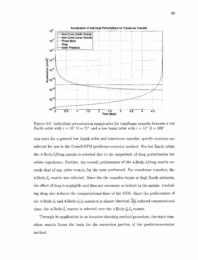
88

Acceleration of Individual Perturbations for Translunar Transfer 10

> 1 0 '

-Non-Conic Earth Gravity -Non-Conic Lunar Gravity Three Body Drag

-Solar Pressure

2 2.5 3 Time (days)

Figure 4.6: Individual perturbation magnitudes for translunar transfer between a low Earth orbit with i = 16° Q = 71° and a low lunar orbit with i = 15° 0 = 100°

tion tests for a general low Earth orbit and translunar transfer, specific matrices are

selected for use in the Cowell-STM predictor-corrector method. For low Earth orbits

the 4-Body J2Drag matrix is selected due to the magnitude of drag perturbation low

orbits experience. Further, the overall performance of the 4-BodyJ2Drag matrix ex

ceeds that of any other matrix for the tests performed. For translunar transfers, the

4-BodyJ2 matrix was selected. Since the the transfers begin at high Earth altitudes,

the effect of drag is negligible and thus not necessary to include in the matrix. Exclud

ing drag also reduces the computational time of the STM. Since the performance of

the 4-BodyJ2 and 4-BodyJ2J3 matrices is almost identical, for reduced computational

time, the 4-BodyJ2 matrix is selected over the 4-Body^J3. matrix.

Through its application in an iterative shooting method procedure, the state tran

sition matrix forms the basis for the correction portion of the predictor-corrector

method.

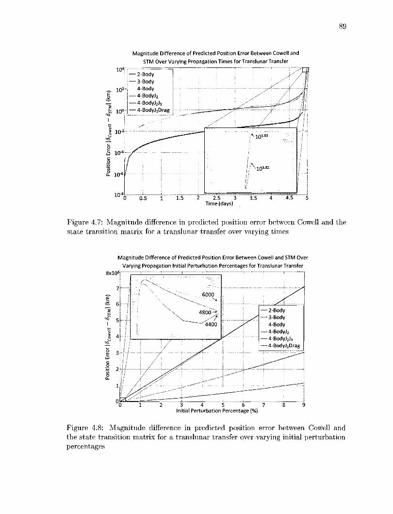
89

Magnitude Difference of Predicted Position Error Between Cowell and

STM Over Varying Propagation Times for Translunar Transfer

104

102

s ,fe 10°

1 10";

o £ 10"4

c o

S. io*

10"8,

— 2-Body — 3-Body

4-Body — 4-BodyJ2

— 4-BodyJ2J3 4_BOC|yj2Drag

.-^' ;

! ! ! ! ! ! ' . ;•••

i - 1 i i ^ s&~ £~

. 1 ~~~; --•'' : ;

7

i i i i

_..-•••''' i __/;_>——P^

; \1 03.83 ^ ;

| ; \ 1 0 3 . 8 2

: 1 . . . ' .

0.5 1.5 2.5 3 Time (days)

3.5 4.5

Figure 4.7: Magnitude difference in predicted position error between Cowell and the state transition matrix for a translunar transfer over varying times

Magnitude Difference of Predicted Position Error Between Cowell and STM Over

Varying Propagation Initial Perturbation Percentages for Translunar Transfer

8xl06

3 4 5 6 7 Initial Perturbation Percentage {%)

Figure 4.8: Magnitude difference in predicted position error between Cowell and the state transition matrix for a translunar transfer over varying initial perturbation percentages

90

4.5 Shooting Method

The shooting method is a technique which numerically solves a two-point boundary

value problem by reducing it to the solution of an initial value problem. For this

research, the boundary value problem focuses on determining the transfer trajectory

between two orbits subject to initial and final constraints. Given an initial state,

(ri, Vi) and time of flight, t2, the state transition matrix is calculated, and the Cowell

propagator integrates the states forward in time (r2int, v2 in t).

Assuming the error in the final position is the only concern, the difference between

the integrated position vector, r2int, a n d the desired position vector, r2, is the error

5r2 = r2 - r2int. (4-73)

To reduce this error, the initial velocity, Vi, must be updated. From Equations 4.8

and 4.9 one finds

$n<5ri + $i25v! = Sr2 (4.74)

and

$215ri + $22^vi = 5v2. (4-75)

Again, because the goal is to only reduce the error in the final position, 5v2 and

Equation 4.75 are of no consequence. Furthermore, it is assumed that the initial

position vector cannot change, thus STI = 0. As a result, Equation 4.74 reduces to

$1 2£V l = 6r2. (4.76)

Solving for 5vi yields

Sv! = [Qu]-1 6r2. (4.77)

91

Thus, at each iteration the new initial delta velocity is updated as

vi,(t+i) = v M + 5vM, (4.78)

where i represents the iteration number. The process iterates until |<5r2| < 1 x 10~6,

or the process has exceeded a number, say forty iterations, in which case the shooting

method has failed to converge. See Figure 4.9 for an illustration of the shooting

method. Figure 4.10 summarizes the shooting method as it applies specifically to

Orbit A

Figure 4.9: Illustration of Lambert shooting method

the translunar and low Earth orbit transfer applications. With the development

of the Cowell-STM predictor-corrector complete, the next two chapters detail the

performance of the tool as applied to these two applications.

92

Translunar Low Earth Orbit

Mufti-conic Propagator (Chapter5)

INPUTS

Lambert 2-Body Problem (Chapter6)

f i

ri,vur2,Vi,t1,t2

Integrate:

*2int — vx

4> = /n(ji,t»i,t2 — t j ) *

Sr2 =r2- r2,

OUTPUTS V-L

f l

NO Sfi = t*12]*1Sr2

" l j = *>1 + St?!

Failed to converge

Figure 4.10: Flow chart summary of the higher order Lambert method formulation

Chapter 5

Translunar Application

The objective of testing translunar transfers is to develop a feasible trajectory between

low Earth orbits (LEO) and low lunar orbits (LLO). The following chapter begins

with an overview of pseudostate theory and its use in approximating three body

trajectories. The next section provides details on JSC's trajectory propagator "EXLX"

that interfaces with the user through an Excel mapping function. The interface

enables the user to select viable transfer parameters based on the initial desired

conditions. The parameters are input into the multi-conic propagator and are used

to acquire an initial guess for the transfer velocity between a low Earth orbit and

the first lunar orbit insertion burn to enter into a circular low lunar orbit, known as

the Translunar Injection (TLI) and Lunar Orbit Insertion (LOI) burns respectively

(see Figure 5.1). Utilizing the shooting method discussed in Section 4.5, the initial

transfer velocity guess is updated to include higher order perturbations. Figure 5.2

summarizes the development of acquiring the final transfer velocity. The remainder

of the chapter discusses the process of selecting the translunar test cases as well as

assesses the performance of the method in generating feasible solutions.

93

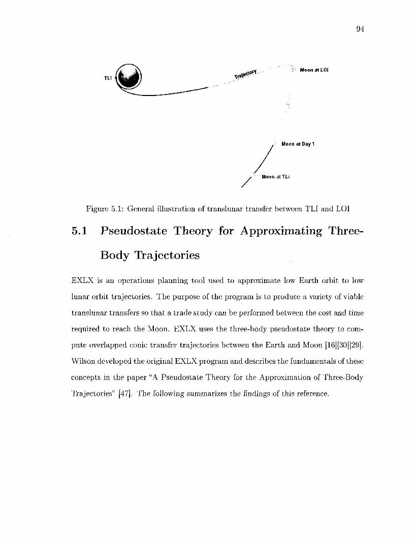
94

, Moon at Day 1

/ Moon at TLi

Figure 5.1: General illustration of translunar transfer between TLI and LOI

5.1 Pseudostate Theory for Approximating Three-

Body Trajectories

EXLX is an operations planning tool used to approximate low Earth orbit to low

lunar orbit trajectories. The purpose of the program is to produce a variety of viable

translunar transfers so that a trade study can be performed between the cost and time

required to reach the Moon. EXLX uses the three-body pseudostate theory to com

pute overlapped conic transfer trajectories between the Earth and Moon [16] [30] [29].

Wilson developed the original EXLX program and describes the fundamentals of these

concepts in the paper "A Pseudostate Theory for the Approximation of Three-Body

Trajectories" [47]. The following summarizes the findings of this reference.

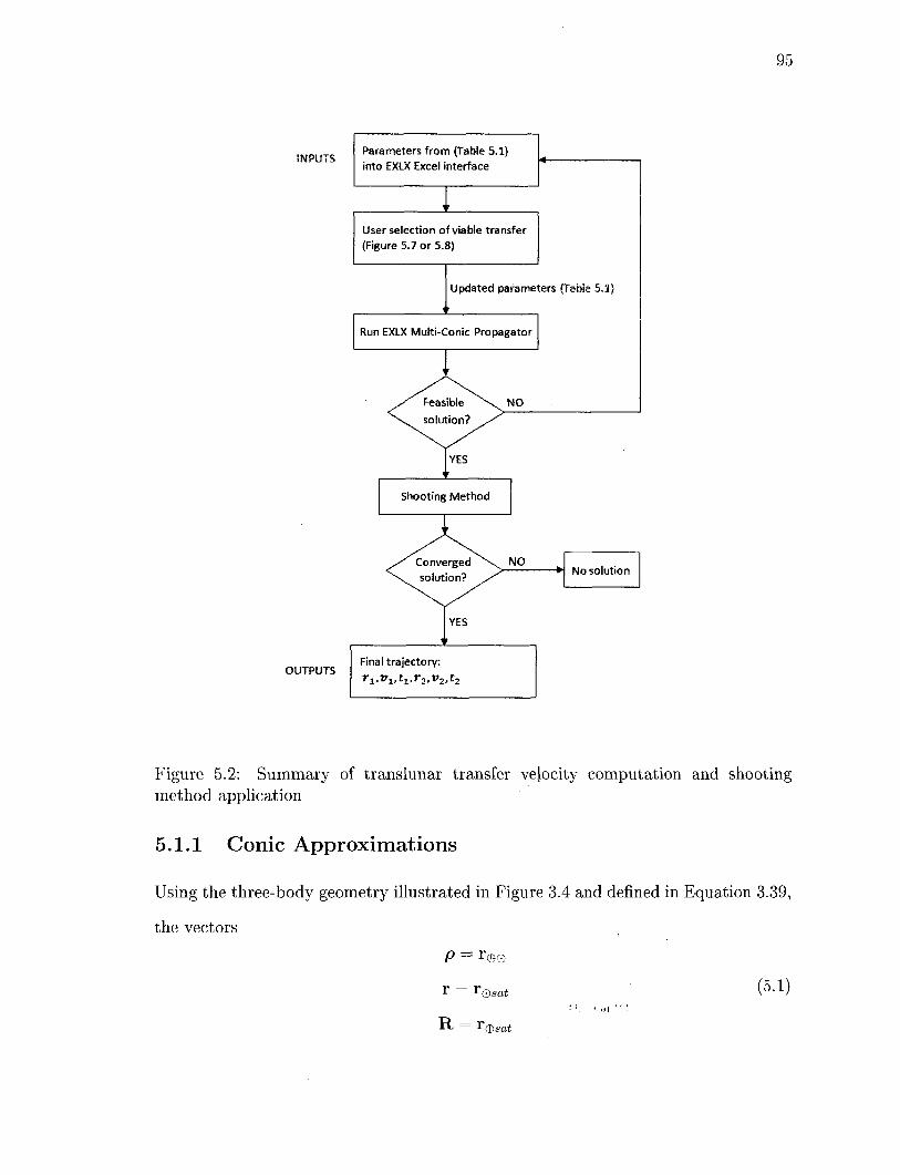
95

INPUTS Parameters from (Table 5.1) into EXLX Excel interface

"

User selection of viable transfer (Figure 5.7 or 5.8)

Updated parameters (Table

Run EXLX Multi-Conic Propagator

> / Feas

\ * . solul

ible \ \ NO

tion? s^

5.1)

YES

Shooting Method

NO

OUTPUTS

YES

Final trajectory: r1,vx,t1,r2,v2,t2

No solution

Figure 5.2: Summary of translunar transfer velocity computation and shooting method application

5.1.1 Conic Approximations

Using the three-body geometry illustrated in Figure 3.4 and defined in Equation 3.39,

the vectors

r = r0 s a t (5.1)

R = Y<3sat

96

are introduced to reduce the complexity of multi-subscripts. For any time tj, the

vectors are related by the equations

R J = p J + r J , (5.2)

and

Rj = Pj + TJ. (5.3)

Assuming the mass of the spacecraft is negligible, the acceleration due to three-body

motion (Equation 3.1) for each vector is

P J = - ( / % +A%) ^ (5-4)

r j , Pj R j r j - - ^ © - 3 +/4B-T" - ^ e - p 3 " . (5-5)

and -5 R j , Tj Pj ,r Rx R - / = - ^ © ^ 3 - + A * 0 ^ - - M © - r - (5-6)

The velocity vectors at two different times, ti and £g, are related by the equations

PE - p / = - 0© + Mo) / f - r ) r f * j . (5-7)

iE-iI = -fiQ I (^Jdtj + n® (-£) dtj - fi® \^)dtj' (5,S)

and

R E - R , = -^ f f i y ^ fe) <&J + Mo j E (Uj dtj- fMQ.J E (^-j dtj. (5.9)

97

The position vectors are related by the equations

PE ~ Pi = fa - ti) Pi - (v® + He) / {-4)dtjdtK, (5.10)

K,

TE-T!= (tE - tj) r7 - //0 ft* ft* ( ^ ) dtj dtK +

*> ftE g {%) ** - *> R: sir ( t ) d t dt

and

RE - Kj = (tE - tt) R, - /% ftE ftK (§f) c?ij di^+

^ J? llK fe) ^ ** - Me J? J? ( g ) *•/ **,

(5.11)

(5.12)

where J and iT are intermediate variables of integration. There are no known closed

form solutions to Equations 5.8, 5.9, 5.11, or 5.12. However Equations 5.7 and 5.10

can be solved using two-body conic equations. Equation 5.7 results in dual definitions

PE~ PI = PI'U*9+HO)E ~ Pn (5-13)

and

PE~ PI = PE~ Pfi^e+Ai©)/-

Similarly Equation 5.10 yields

PE ~ Pi = Pi(^+m)E - Pn (5-14)

and

PE~ PI = PE~ PE(tim+nQ)i-

Here the compound subscripts refer to a vector resulting from the conic propagation

of a base-point state vector. The first element of the subscript identifies the base-

point vector, the second element describes the gravitational constant used in the conic

98

propagation, and the third element is the time component of the conically propagated

state vector. Thus, in Equation 5.13, the term pi^9+flQ)E refers to the velocity

vector found by propagating the base-point state vector from time tj, ( p ^ p j ) , along

a conic trajectory to time £# using the combined Earth-Moon gravitational parameter

P® + PQ-

When the spacecraft is very close to the Moon the sum of the last two terms in

Equation 5.5 is close to zero. By removing these two terms Equation 5.5 has the

same form as Equation 5.4 and thus the two-body conic approximations in Equations

5.13 and 5.14 can be applied to r as well. The selenocentric conic approximations for

velocity are then

tE TinoJ iE - ii = rIlM E - r 7 = -p& / - T ^ - dtj, (5.15) ti \rln0J

and

rE - r 7 = iE - rE„ei = -pQ / ~Y^- dtj. (5.16)

The approximations for position are

rE-rI^rIfMOE-rI = (tE-tI)rI-iie [ * I * lTJpl\dtjdtK, (5.17) Ju Jtj yifiQjJ

and

^E ~ r / = YE - rEfMsi = {tE ~ ti) *Emi - P-o / _|^©£ | dtjdtK. (5.18) Jt! Jti \rEfiQjJ

The selenocentric conic approximations can be used whenever the spacecraft is close

to the Moon within the time interval (£/, tE).

A similar set of approximations can be made when the spacecraft is near the

Earth. With this condition the sum of the last two terms in Equation 5.6 are close to

zero and thus can be omitted to estimate the geocentric conic approximations. For

99

velocity these equations are

tE / R/UfflJ

and

HE — R/ = R / ^ B — R/ = —^e / p 3 ] dtj, (5.19)

HE — R/ — R B — RE/X®/ = — f1® / p 3 ^ J ! (5.20) Itj \REfimJ

and for the position vectors the associated equations are

KE - R7 ^ R7/iffiE -RI = (tE-tI)RI-ti® I* I* I ^ ^ J dijd**, (5.21)

and

R B — R/ — R E — Rfi/i®/ = (tE — ti) it-Eii®! — /% / / p3 I dtjdtK. (5.22)

Again, the geocentric conic approximations can only be made when the spacecraft is

near the Earth within the time interval (£/,£#).

Distances representative of "near the Moon" and "near the Earth" are a func

tion of each body's respective sphere of influence (SOI) [7]. The Moon's sphere of

influence is usually defined as some value between 9 and 14 Earth radii from the

center of the Moon. The number is based on the observations of when selenocen-

tric conic approximations more accurately define spacecraft motion then geocentric

conic approximations. The classical method of patched conies as developed by Egorov

[21] assumes that selenocentric conic approximations are used when the spacecraft is

within the sphere of influence of the Moon, and geocentric conic approximations are

used to describe motion outside of the lunar sphere of influence. On the Earth to

Moon transfer, the spacecraft is initially propagated along the geocentric conic tra

jectory until it reaches the Moon's sphere of influence. At this point the state vector

is transformed from geocentric coordinates to selenocentric coordinates (see Section

100

3.3.2) and the propagation continues along the selenocentric conic trajectory until

the desired terminal point is reached.

5.1.2 Overlapped Conic Approximation

The disadvantage of the classic patched conic technique is that the omitted terms

in Equations 5.5 and 5.6 can possess large values in the region near the Moon's

sphere of influence. In this case, significant errors result from the conic approximation

technique. The overlapped conic approximation is an alternative method that does

not neglect the final terms from Equations 5.5 and 5.6 but still retains the simplicity

of the classic two-body approach [39].

To set up the problem assume an interior point / that is located within the Moon's

sphere of influence and an exterior point E that is located within the vicinity of the

Moon but outside of the sphere of influence as depicted in Figure 5.3. For this reason

the interior point is defined with respect to selenocentric coordinates, denoted by the

symbol a

oj = (h, n, rj), (5.23)

and the exterior point is defined with respect to geocentric coordinates, denoted by

the symbol £

ZE= (tE,RE,REy (5.24)

A relationship is needed between Equations 5.23 and 5.24 where tp(B < tj < tE < tpQ

or t^ > ti > tE > tpQ. Here tp9 refers to the perigee passage time and tpQ refers

to pericynthion, or the time of periapse passage for the lunar orbit. This restriction

requires no periapse passage between the terminal points, ensuring that the conic

approximations remain valid. At periapse points the propagation must be switched

from exterior-to-interior to interior-to-exterior or vise versa depending on the direction

of the transfer. The periapse restriction does not mean the overlapped conic approach

101

Moon SOI, tE Moon SOI, t ;

Earth

k^k

Figure 5.3: Definition of interior and exterior points for overlapped conic approximation

cannot be utilized for transfers that pass through periapse points, only that such

transfers require more than one step.

The first step in determining a relationship between the selenocentric interior

point and the geocentric exterior point begins with finding approximate solutions for

Equations 5.9 and 5.12 which have no known closed-form solutions. For the integral of

( ^ ) it is expected that the geocentric conic approximation of R j will be reasonably

accurate with a proper selection of the base-point vector. Since the exterior point

is closer to the Earth then the interior point, it makes sense that R j = R#M ej is

a better approximation then R j = HImj. Substituting this value in and using the

102

relationship found in Equation 5.20, the first single integral in Equation 5.9 becomes

ftE (RE^J

Jti \RE^J -/% fj (^ ) dtj * -to J " ( ^ ^ ) dtj = RE- RE^I- (5-2 5)

Using Equation 5.22, the double integral in Equation 5.12 becomes

-Me JlE £" ( f ) dtj dtK - ^ Si? £ ( ^ ) dtj dtK

RE — REH®I — At/sR-B/i®/,

(5.26)

where AtiE = tE — tj. A similar approximation is made for the integral of ( j . Since

the interior point is closer to the Moon the following selenocentric conic approximation

is made Yj = YI^QJ. Substituting this value in and using the relationship found in

Equation 5.15, the single integral in Equation 5.9 becomes

-to fB (r4) dtj S* -to fE [ ^ ) dtj = rIfleE - r7. (5.27) Jtj \ r j J Jti \TI^QJ )

Using Equation 5.17, the double integral in Equation 5.12 becomes

- s:: c fa)** «* * -»° s,r s,r (%*) * <** * (6 28)

r / / i 0 £ - 17 - AtIErj.

The integral for (-%•) is found from Equations 5.7 and 5.10 where

-A*0 Jt E (jf} dtj = eApIE, (5.29)

and

-to [E [K (^r)dtjdtK = e [ApIE - AtIEPl] (5.30)

103

with ApIE = pE — pj, A p / E = pE — pr, and e is the constant

e = _ ^ L _ _ . (5.31)

Substituting Equations 5.5, 5.25, 5.27, and 5.29 into Equation 5.9 yields

Rfi/iffi/ = Pi + *inoE + ep / B . (5.32)

Further, substituting Equations 5.2, 5.3, 5.26, 5.28, 5.30, and 5.32 into Equation 5.12

yields

RjS/ieJ - Pi + r % E ~ AtIErIliQE - e {P/ - [ps - A t / B p B ] } . (5.33)

Equations 5.32 and 5.33 can be rearranged to derive

YI^QE = R ^ j - P i - e A p / e , (5-34)

and

r/MQjE; ^ B.EH@I ~Pi + ktIErIllQE + e{pT- [pE - AtIEpE}} . (5.35)

If the interior state vector, oj from Equation 5.23, is known, then rIflQE and r/M0E

can be calculated by selenocentric conic propagation to time tE. The lunar positions

and velocities at the two terminal points, p 7 , pT, pE, and pE can be found through

an ephemeris program such as SPICE (Section 3.2) or by conic propagation (Section

2.2). Thus Equations 5.32 and 5.33 are used to find the state vector in closed-form,

ZEU®! = \tl,'R'Eij,eI,~R'Eii(Bl) • (5.36)

104

Since conic propagation is reversible, the following equation

~R-{Emi)mE = R £ ( 5 - 3 7 )

holds. Hence the closed-form approximate solution of £g is found by propagating

£EII®I along a geocentric conic to time tE.

Conversely, if the exterior state vector, £E, is known, then R£ / l 0 / and R ^ e / can

be computed using geocentric conic propagation to time £/. In this case, Equations

5.34 and 5.35 are applied to find the state vector

E) • (5-38)

The closed-form approximate solution of 07 is then found by propagating crItlQE along

a selenocentric conic to time £/.

If the interval between tj and tE is broken into many segments, Equations 5.32

and 5.33 can be applied in each subsequent interval. This develops an approximate

numerical integration algorithm which enables both large integration steps and main

tains good accuracy. The terms in Equations 5.32 and 5.33 multiplied by the factor e

are integrals of the three-body perturbing acceleration and thus provide a first order

rectification to the conic orbits between propagation steps. Additional rectification

terms are added to Equations 5.32 and 5.33 to account for J^ and solar perturbations

as shown in Reference [13].

For preliminary translunar mission trade studies, the ability to take large integra

tion steps, such as perigee to pericynthion, is desired so that many trajectories may

be evaluated. For these problems, perturbations due to the sun and an oblate Earth

are ignored. Without these major perturbations the rectification terms in Equations

5.32 and 5.33 can be omitted without significantly increasing the error of the ap

proximation. The error remains small as long as the definition of the lunar vicinity

105

remains within a selenocentric "pseudostate transformation sphere" (PTS) having a

radius of 20 to 40 Earth radii. Here the word "pseudostate" derives from the phrase

"pseudo target aiming point" which refers to a point a translunar transfer trajectory

approximated as an ellipse would pass through [38]. The pseudostate transformation

sphere is centered on and moves with the Moon. With a radius larger than that

denned by the Moon's sphere of influence, the PTS expands into Earth's sphere of

influence, allowing the selenocentric conic to overlap a portion of the geocentric conic.

Outside of this sphere, only geocentric conic propagation is used to define the motion

of the spacecraft.

The simplified overlapped conic equations form the basis for the pseudostate the

ory discussed next.

5.1.3 Pseudostate Theory

When the rectification terms are removed from Equations 5.32 and 5.33 the equations

fWeJ = Pi + ri^oE, (5.39)

and

Ri5/i©J = Pi + rinQE - AtiEii„QE (5.40)

are returned. In addition to its use as an algorithm for propagating known state

vectors, the pseudostate theory provides the most value in applying the overlapped

conic approximation to boundary value problems using procedures that do not require

a first-guess state vector.

Pseudostate terminals are points on the trajectory at which the overlapped conic

segments begin and end. Each segment has an interior and exterior terminal. Interior

terminals may be the initial or final point in the trajectory as illustrated in Figure

5.4, or a pericynthion point as illustrated in Figure 5.5. Exterior terminals may be

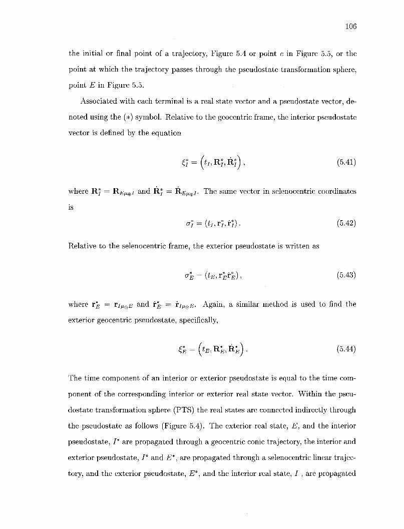
106

the initial or final point of a trajectory, Figure 5.4 or point e in Figure 5.5, or the

point at which the trajectory passes through the pseudostate transformation sphere,

point E in Figure 5.5.

Associated with each terminal is a real state vector and a pseudostate vector, de

noted using the (*) symbol. Relative to the geocentric frame, the interior pseudostate

vector is defined by the equation

£ ; = ( t 7 , R * , R * ) , (5.41)

where R} = R.EMffl/ and R} = R E ^ / . The same vector in selenocentric coordinates

is

a; = (t7 ,r*,f}). (5.42)

Relative to the selenocentric frame, the exterior pseudostate is written as

aE = (tE, vErE), (5.43)

where r*E = TI^QE and rE = YI^E- Again, a similar method is used to find the

exterior geocentric pseudostate, specifically,

CE = (tE)R*E,KE) . (5.44)

The time component of an interior or exterior pseudostate is equal to the time com

ponent of the corresponding interior or exterior real state vector. Within the pseu

dostate transformation sphere (PTS) the real states are connected indirectly through

the pseudostate as follows (Figure 5.4). The exterior real state, E, and the interior

pseudostate, I* are propagated through a geocentric conic trajectory, the interior and

exterior pseudostate, /* and E*, are propagated through a selenocentric linear trajec

tory, and the exterior pseudostate, E*, and the interior real state, / , are propagated

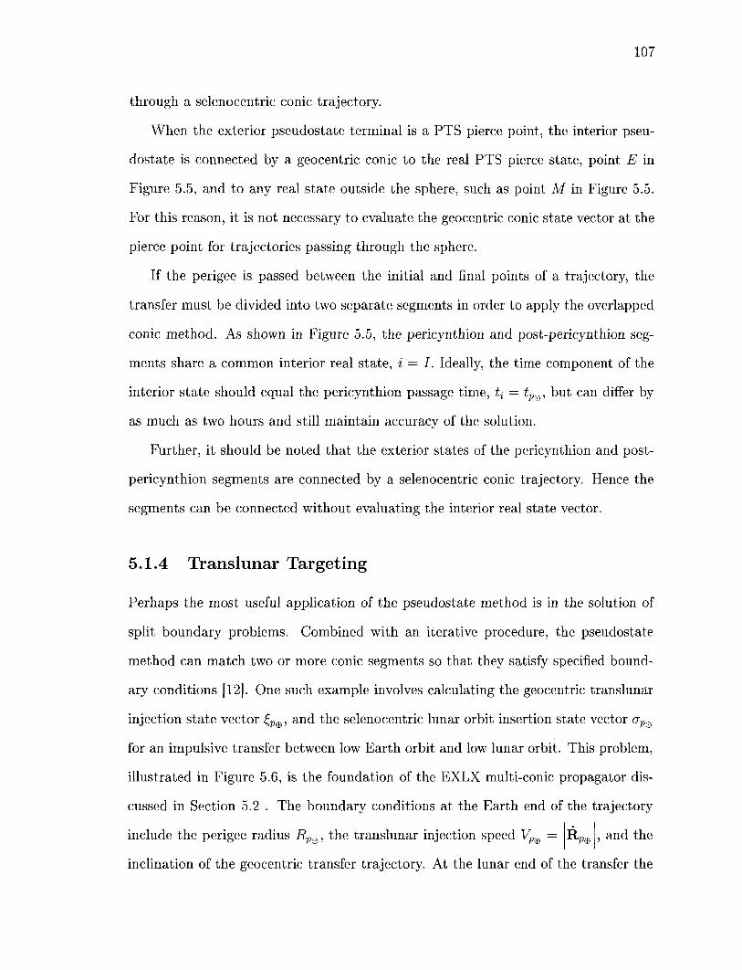
107

through a selenocentric conic trajectory.

When the exterior pseudostate terminal is a PTS pierce point, the interior pseu-

dostate is connected by a geocentric conic to the real PTS pierce state, point E in

Figure 5.5, and to any real state outside the sphere, such as point M in Figure 5.5.

For this reason, it is not necessary to evaluate the geocentric conic state vector at the

pierce point for trajectories passing through the sphere.

If the perigee is passed between the initial and final points of a trajectory, the

transfer must be divided into two separate segments in order to apply the overlapped

conic method. As shown in Figure 5.5, the pericynthion and post-pericynthion seg

ments share a common interior real state, i = I. Ideally, the time component of the

interior state should equal the pericynthion passage time, tj = tPe, but can differ by

as much as two hours and still maintain accuracy of the solution.

Further, it should be noted that the exterior states of the pericynthion and post-

pericynthion segments are connected by a selenocentric conic trajectory. Hence the

segments can be connected without evaluating the interior real state vector.

5.1.4 Translunar Targeting

Perhaps the most useful application of the pseudostate method is in the solution of

split boundary problems. Combined with an iterative procedure, the pseudostate

method can match two or more conic segments so that they satisfy specified bound

ary conditions [12]. One such example involves calculating the geocentric translunar

injection state vector £Pffi, and the selenocentric lunar orbit insertion state vector aPQ

for an impulsive transfer between low Earth orbit and low lunar orbit. This problem,

illustrated in Figure 5.6, is the foundation of the EXLX multi-conic propagator dis

cussed in Section 5.2 . The boundary conditions at the Earth end of the trajectory

include the perigee radius RpB, the translunar injection speed Vm = R„ , and the

inclination of the geocentric transfer trajectory. At the lunar end of the transfer the

108

PTS, t, Real Geocentric Trajectory

Geocentric Conic

Selenocentric Conic

Selenocentric Linear Trajectory

Earth

Figure 5.4: Pseudostate terminals for a short segment of a translunar trajectory

boundary conditions include the time of orbit insertion tm = U, the pericynthion

radius rPQ = |r,|, and the restriction that the lunar orbit plane contain a given vector

TL- The problem is solved by iterating on R*, the geocentric interior pseudostate po

sition vector. For the first iteration R* = pi which can be found from an ephemeris

program.

If VL2m < 4^-, the geocentric conic is elliptical and has an apogee distance of RA-

In this case it is assumed that |R*| = R* < RA for any value of R* used in the

iterative process. It is also assumed that the declination of R* is never greater then

the geocentric orbit inclination. If these requirements are met, there exist geocentric

conies that pass through R} which satisfy the initial boundary conditions on Rp®,

Vp®, and inclination. For each possible conic the quantities for R*, ip®, Rp®, and

Rp® are computed explicitly. It is assumed selection criteria are specified, such as the

azimuth angle sign, to determine which of the possible conies is the unique solution.

Having calculated R* , Equation 5.3 is used to find r*. Based on the earlier

109

PTS, tt = t, ~ Real Geocentric Trajectory

- Geocentric Conic

- Selenocentric Conic

- Selenocentric Linear Trajectory

Earth

Figure 5.5: Pseudostate terminals for a circumlunar segment of a translunar trajectory

assumption that R* = p^ on the first iteration r* is not exact. However, the assump

tion is accurate enough to compute a new estimate R* for the interior pseudostate

position using the following equations.

The linear relationship between interior and exterior pseudostates mentioned ear

lier defines r* = r*. The remaining components of the exterior pseudostate, te and r*

are found by applying the lunar boundary conditions. For this case, the magnitude

of r* is equal to the pseudostate transformation sphere radius, rs. The equation for

specific mechanical energy gives

VPO = \<f - ^ 2A% '©

' p©

(5.45)

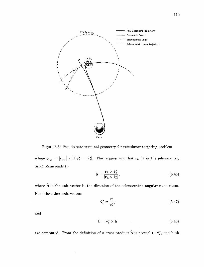
110

PTS, t ( = t Pa

Earth

- Real Geocentric Trajectory

- Geocentric Conic

- Selenocentric Conic

- Selenocentric Linear Trajectory

Figure 5.6: Pseudostate terminal geometry for translunar targeting problem

where vPe = |rPQ| and v\ = |r*|. The requirement that TL lie in the selenocentric

orbit plane leads to

r L x r * (5.46) \rL x r*|

where h is the unit vector in the direction of the selenocentric angular momentum.

Next the other unit vectors

V e = (5.47)

and

b = v* x h (5.48)

are computed. From the definition of a cross product b is normal to v*, and both

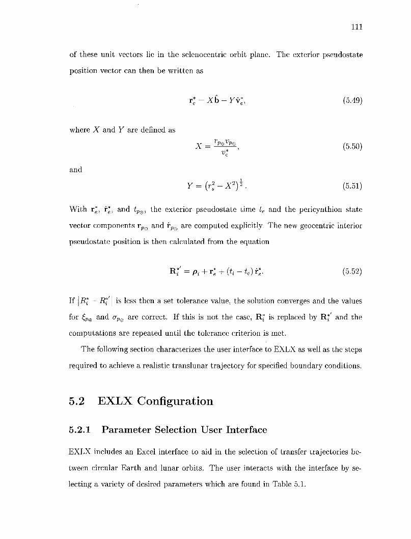
I l l

of these unit vectors lie in the selenocentric orbit plane. The exterior pseudostate

position vector can then be written as

r*e = Xb - Yv*e, (5.49)

where X and Y are defined as

and

X = ^ ^ , (5.50) v*

Y=(r2s-Xy. (5.51)

With r*, r*, and tPe, the exterior pseudostate time te and the pericynthion state

vector components rP0 and rPQ are computed explicitly. The new geocentric interior

pseudostate position is then calculated from the equation

R*' = Pi + re* + (U - te) re*. (5.52)

If \R* — R* | is less then a set tolerance value, the solution converges and the values

for £Pffl and aPQ are correct. If this is not the case, R | is replaced by R* and the

computations are repeated until the tolerance criterion is met.

The following section characterizes the user interface to EXLX as well as the steps

required to achieve a realistic translunar trajectory for specified boundary conditions.

5.2 EXLX Configuration

5.2.1 Parameter Selection User Interface

EXLX includes an Excel interface to aid in the selection of transfer trajectories be

tween circular Earth and lunar orbits. The user interacts with the interface by se

lecting a variety of desired parameters which are found in Table 5.1.

112

Parameter Date of MET Zero (origin of Mission Elapsed Time scale)

Altitude of Earth circular parking orbit Inclination of Earth orbit (iffi)

Right ascension of ascending node (He) Time of Earth orbit ascending node definition wrt MET Zero

Time of Earth orbit departure wrt MET Zero Time of lunar orbit insertion wrt MET Zero

Perisel altitude of plane change ellipse Orbit period of plane-change ellipse

Altitude of lunar circular parking orbit Selenographic inclination of lunar orbit (i0)

Selenographic longitude of lunar orbit ascending node (fi©) Time of lunar orbit ascending node definition wrt MET Zero

Units Year\Month\d\hh:mm

km deg deg

d\hh:mm d\hh:mm d\hh:mm

km d\hh:mm

km deg deg

d\hh:mm

Table 5.1: User selected parameters for EXLX Excel interface for three-burn sequence

In addition to the parameters just listed, the user has the option of "flying out"

single or triple impulse maneuvers. For three-impulse cases, the lunar orbit insertion

time is considered the first impulse which establishes a selenocentric plane-change

ellipse. The parameters in Table 5.1 refer to a three-impulse burn. In the case of a

single impulse transfer, the "perisel altitude of plane-change ellipse" and "orbit-period

of plane change ellipse" parameters no longer exist and instead are replaced with

a "low limit on perisel altitude of approach hyperbola" option. EXLX also has the

option to constrain any output variable with lower and upper bounds. For example,

the user may put restrictions on the impulsive translunar injection azimuth angle or

the time between the translunar injection and the lunar orbit insertion.

After the setup parameters are selected, the interface maps the resulting data.

The mapping takes the form of a two dimensional scan space represented by a matrix.

Though EXLX can handle a variety of scan types, for this research the scans were

limited to lunar parking orbit accessibility scans and timetable scans. Lunar parking

orbit accessibility scans haves axes which represent various longitude of the ascending

nodes, fi0, and orbit inclinations, i&, for possible lunar parking orbits. Timetable

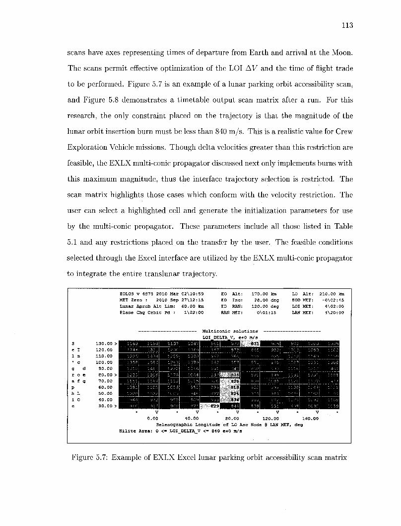
113

scans have axes representing times of departure from Earth and arrival at the Moon.

The scans permit effective optimization of the LOI AV and the time of flight trade

to be performed. Figure 5.7 is an example of a lunar parking orbit accessibility scan,

and Figure 5.8 demonstrates a timetable output scan matrix after a run. For this

research, the only constraint placed on the trajectory is that the magnitude of the

lunar orbit insertion burn must be less than 840 m/s. This is a realistic value for Crew

Exploration Vehicle missions. Though delta velocities greater than this restriction are

feasible, the EXLX multi-conic propagator discussed next only implements burns with

this maximum magnitude, thus the interface trajectory selection is restricted. The

scan matrix highlights those cases which conform with the velocity restriction. The

user can select a highlighted cell and generate the initialization parameters for use

by the multi-conic propagator. These parameters include all those listed in Table

5.1 and any restrictions placed on the transfer by the user. The feasible conditions

selected through the Excel interface are utilized by the EXLX multi-conic propagator

to integrate the entire translunar trajectory.

Figure 5.7: Example of EXLX Excel lunar parking orbit accessibility scan matrix

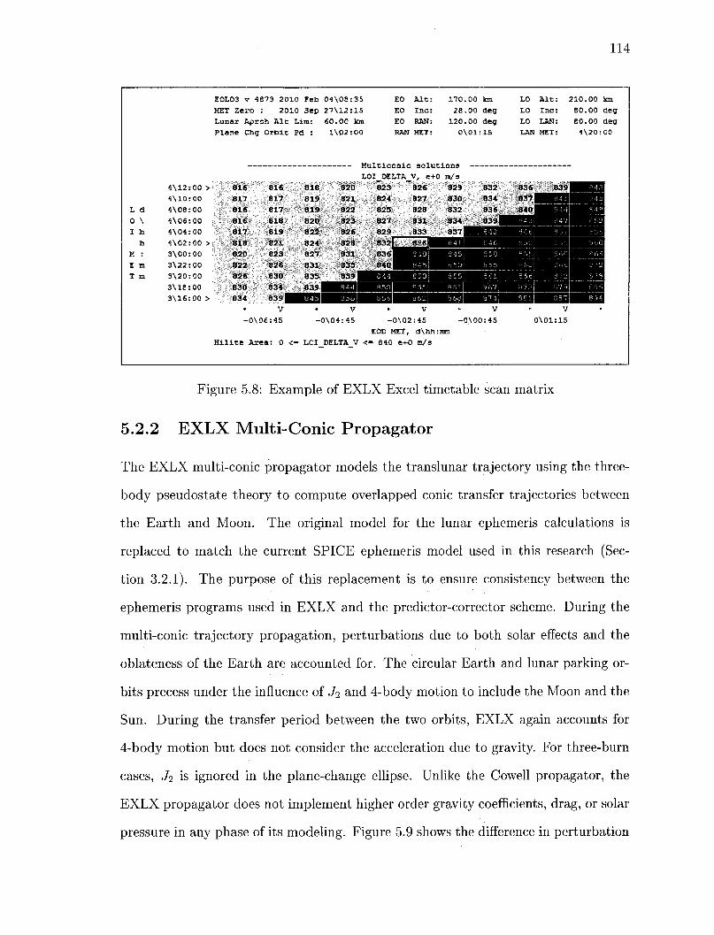
114

L

0

I

M

£

T

d

\

m

m

4\12

4\10

4\08

4\Q6

4\04

4\02

3\00

3\22

3\20

3\18

3\16

00 > 00

00

00

00

00 >

00

00

00

00

00 >

EOL03 v 4873 2010

MET Zero 2010

Feb

Sep

Lunar Aprch Alt Lim:

Plane Chg

816 817

816

816

817

818

820

822

826

830

834

•

Orbit Pd :

816

817

817

818

819

821

823

826

830

818

819

819

820

822

824

827

831

835

834 839

839K$S V

-0\06:4S

Hilite Are a: 0 <=

• -

LOI_

04\08:35 27\12:15

60.00 km

1\02:00

E0

E0 EO RAH

LOI_DELTA_

820 821

822

823

826

828

831

835

839 •

IB V

D\04:45

_DELTA_V <

823

824 825

827 sss

840

• • —

Alt:

Inc:

RAN: MET:

170

28

120

00

00 00

0V01

SO 2. tit

V, e+0 826

827 828

831

833

83fiM

V

Q\Q2:45

EOD MET,

- 840

d\Mi:

e+0 m/s

m/s

829

830 832

834

837

«

km

deg deg

IS

832

834

836

8391

V

-0\00:4S

EHTE

LO Alt: 210.00

LO Inc: 80.00

LO LAN: 80.00

LAN MET: 4\20

836 839 ^ H Q 837^^^O^^S fMO^^^ffl^^Q

V

0\01:15

km

deg

deg

00

•

Figure 5.8: Example of EXLX Excel timetable scan matrix

5.2.2 EXLX Multi-Conic Propagator

The EXLX multi-conic propagator models the translunar trajectory using the three-

body pseudostate theory to compute overlapped conic transfer trajectories between

the Earth and Moon. The original model for the lunar ephemeris calculations is

replaced to match the current SPICE ephemeris model used in this research (Sec

tion 3.2.1). The purpose of this replacement is to ensure consistency between the

ephemeris programs used in EXLX and the predictor-corrector scheme. During the

multi-conic trajectory propagation, perturbations due to both solar effects and the

oblateness of the Earth are accounted for. The circular Earth and lunar parking or

bits precess under the influence of Ji and 4-body motion to include the Moon and the

Sun. During the transfer period between the two orbits, EXLX again accounts for

4-body motion but does not consider the acceleration due to gravity. For three-burn

cases, J% is ignored in the plane-change ellipse. Unlike the Cowell propagator, the

EXLX propagator does not implement higher order gravity coefficients, drag, or solar

pressure in any phase of its modeling. Figure 5.9 shows the difference in perturbation

115

approximations of each flight phase for the EXLX and Cowell propagators.

LEO transfer LLO

4-Body Motion Low Order Gravity: J2

4-Body Motion 4-Body Motion Low Order Gravity: J2

4-Body Motion High Order Gravity: J2.9

Atmospheric Drag Solar Radiation





Figure 5.9: Perturbation dynamics applied in each flight phase for the EXLX and Cowell propagators over a translunar trajectory

In calculating the impulsive translunar injection burn, EXLX solves Lambert's

problem (Section 6.1) with the position in the lunar parking orbit optimized for

minimum delta velocity.

Using the viable parameters selected from the Excel interface, the EXLX multi-

conic propagator applies an overlapped conic approximation to determine a feasible

trajectory for a translunar mission. The final trajectory output from EXLX includes

the states from the Mean Epoch Time through the third lunar insertion burn (LOI3).

Avoiding the complexity of adding thrust acceleration to the Cowell propagator, the

initial position and velocity of the vehicle is set to the states: produced by EXLX at the

translunar insertion (TLI) burn. The final states are taken, as those at the first lunar

orbit insertion burn (LOU). When the EXLX trajectory is flown out using the high

fidelity Cowell propagator, the integrated states miss the desired final position due

to the limited accuracy of the perturbation models utilized by the EXLX multi-conic

propagator. To produce a more accurate final state, assuming the initial position

is fixed, the initial velocity must be updated. The velocity, correction is computed

through the error state transition matrix and the updated states are flown out with

the Cowell propagator again. This iterative shooting method process continues until

116

the integrated position value comes within a set tolerance of the desired final position.

The method just described summarizes the process of acquiring the most ac

curate translunar transfer velocities given the perturbation models applied in the

Cowell-STM predictor-corrector. The following section details the process of select

ing translunar test cases.

5.3 Test Case Selection

The process in selecting the translunar test cases begins with choosing which param

eters to hold constant and which to vary for each case. Preliminary testing illustrates

that holding the Earth and Moon orbits constant and changing the date does not

vary the transfer orbit enough to thoroughly test a variety of possible cases. This is

because the geometry of the Moon with respect to the Earth stays relatively the same

over the period of a year. Although the Moon's declination will change from ±28.5°

as a result of the tilt of the Earth (23.5°) and Moon (5°) with respect to the ecliptic

plane (Figure 5.10), the variation is not enough to greatly change the transfer trajec

tory between two constant Earth and lunar orbits. Hence it is not the position of the

Figure 5.10: Tilt of the Earth and Moon with respect to the ecliptic plane

117

Moon that greatly affects the transfer trajectory but the characteristics of the Earth

and lunar parking orbits. As a result, from Table 5.1 the Earth orbit inclination, i®,

and right ascension of ascending node, f2e, as well as the lunar orbit inclination, i&,

and longitude of ascending node, f20, were the four parameters selected to indepen

dently vary. The remainder of the parameters from Table 5.1 were set to the values

in Table 5.2 for all test cases.

Parameter Date of MET Zero (origin of Mission Elapsed Time scale)

Altitude of Earth circular parking orbit Inclination of Earth orbit (ie)

Right ascension of ascending node (Jl®) Time of Earth orbit ascending node definition wrt MET Zero

Time of Earth orbit departure wrt MET Zero Time of lunar orbit insertion wrt MET Zero

Perisel altitude of plane change ellipse Orbit period of plane-change ellipse

Altitude of lunar circular parking orbit Selenographic inclination of lunar orbit (iQ)

Selenographic longitude of lunar orbit ascending node (Sl0) Time of lunar orbit ascending node definition wrt MET Zero

Value February 20, 2012 12:00

170 km 0° - 360° (deg) 0° - 360° (deg)

0\01:30 0\00:30 5\00:00 50 km 1\00:00 200 km

0° - 360° (deg) 0° - 360° (deg)

4\20:00

Table 5.2: Selected parameter values for translunar test cases

Though the translunar cases were selected for triple impulse maneuvers, only the

first burn, LOU, is considered. Since integrating multiple burns into the predictor-

corrector algorithm would require multi-level targeting, for simplicity only the first

burn is calculated. Due to the fact that the Excel interface to EXLX does not support

changing any other orbital elements, such as eccentricity or true anomaly, these values

remain constant throughout the test cases. For the set time of flight of 5 days and

the maximum velocity constraint of 840 m/s on the LOI AV, not all combinations

of geocentric and selenocentric inclinations and nodes are possible. To develop an

initial idea of the parameter ranges that are feasible, multiple scans are performed

across lunar inclinations from 0° — 360° and ascending nodes from 0° — 360° for a

variety of initial Earth orbits. Each scan produces a 360° x 360° matrix of LOI AV's

118

which are plotted as contours. Figure 5.11 is an example of one scan for an initial

Earth orbit with ze = 0° and £)e = 0°. The white contour line plotted on the figure

represents the isoline ranging from 0-840 m/s. These lines mark the the boundaries

of feasible lunar parameter regions for the particular Earth orbit tested. Thus, for

this specific initial Earth orbit, the only feasible lunar orbits are near equatorial

(i© = 0° = 360° or 180°) at any node, or any inclination at either the ascending

or descending node (f2Q = 90°or 270°). Due to the difficulty of analyzing multiple

Lunar Orbit Insertion AV for Earth Orbit with i = 0° and H = 0'

meet the constraint of AVmax = 840 km/s

contour plots on one figure, for comparison purposes only the isoline at 840 m/s is

plotted over the varying initial Earth orbits. Figure 5.12 shows the results for a few

of the initial Earth orbits tested, with the first data set representing the information

plotted in Figure 5.11. It is clear that the trend of feasible lunar parameters from

Figure 5.11 is carried over to some degree for each initial Earth orbit tested. Where

some initial Earth orbits lend themselves to a variety of possible final lunar orbits, such

119

as those with initial condition combinations of i@ = 45° and Q e = 45° or ze = 315°

and QQ = 135°, others require very specific lunar conditions to result in a feasible

trajectory. The small contour regions representative of an Earth orbit with i© = 90°

and Q® = 315° is one example in Figure 5.12. To see the results broken down by each

Earth orbit analyzed refer to Appendix A. The trends highlighted in Figure 5.12 and

Feasible Lunar Parameters for Earth Orbit o f Varying Inclinations and Ascending Nodes

30 50 100 150 200 250 300 350 Selenographic Longitude of Ascending Node (deg)

Figure 5.12: Contour plot of feasible lunar orbit parameters for varying initial Earth orbit parameters

more specifically in Appendix Figures A.1-A.8 provide guidelines for selecting Earth

and lunar parameters for each test case. Once a feasible combination of parameters

is selected, the values are utilized by the EXLX multi-conic process to propagate the

trajectory. For a few set of feasible Earth and lunar conditions selected from the

Excel interface, the multi-conic propagator does not converge. This is a result of

an iteration number limitation on solving the procedure described in Section 5.1.4.

In trying to propagate the conic with a J2 correction, the value \R* — R* | does not

reduce below the set tolerance of 1 x 10~8 before the maximum number of iterations,

29, is reached. Theorizing that convergence is within a few iterations and that the

parameters only need slight adjustments, the lunar parameters are run through the

120

multi-conic method again with a change of ±3°. This simple correction addresses

the convergence issue. For those solutions that do converge, the final state vector is

checked for any large discontinuities by visually inspecting the plotted trajectory. For

a few cases, the outputted trajectories contain discontinuities that force the states to

change unrealistically in short periods of time. Cases such as these are eliminated as

infeasible.

The user interface for EXLX preclude a large number of Monte Carlo runs. For

this reason only 110 cases are tested. See Appendix B for how this sample size is

selected. The distribution of the feasible parameters selected for the 110 Earth and

Moon orbits (see Appendix C for the details of each test case) is plotted in Figure 5.13.

Also plotted on the figure is the most encompassing boundary line from Figure 5.12.

Clearly, most of the lunar parameters are within the plotted contour lines. Those

that are outside of the isolines in Figure 5.13 are not necessarily in the "infeasible"

region, since the plot is only a generalized representation of what the exact contour

may look like.

From the trends discussed earlier, it is deduced most of the Earth inclinations

are restricted to prograde orbits as delineated by the horizontal lines in Figure 5.13.

Prograde and retrograde orbits are distinguished by the direction of their rotation

about the central body. In a prograde orbit, the vehicle rotates counterclockwise

around the central body as viewed from the north pole, thus the orbits have inclina

tions between 0° — 90°. Retrograde orbits on the other hand, rotate clockwise around

the central body as viewed from the north pole, thus they have inclinations between

90° — 180° [10]. Though the inclination ranges just described are the most common

for prograde/retrograde motion, inclinations can exist between 180° — 360°. Orbits

with inclinations between 180° — 270° are the same as the prograde orbits between

0° — 90° except they have retrograde motion. Likewise, orbits with inclinations be

tween 270° — 360° are the same as orbits between 90° — 180° except with prograde

121

motion.

Range of Inclinations and Ascending Nodes for Tested Geocentric and Selenocentric Orbits

Ascending Node (deg)

Figure 5.13: Distribution of Earth and lunar orbital elements for 110 test cases

5.4 Results and Analysis

All 110 translunar test cases converge using the Cowell-STM predictor-corrector

method. A histogram of the results is found in Figure 5.14. Only three cases are

outside the 1.5 interquartile range and they have iteration counts of 30, 31, and 34

respectively. The convergence trend of a number of the cases as well as the outlier

cases is highlighted in Figure 5.15. Two trends appear to cause a larger than average

number of iterations. It seems that the quicker the shooting method drops \AR\ be

low 100 km, the quicker the case converges. Those cases that bounce back and forth,

oscillating between 1,000-10,000 km have the most difficulty converging. Though this

trend occurs frequently, it is not always the case. As seen in Figure 5.15 with the

outlier case that requires 30 iterations, \AR\ drops below 100 km at 7 iterations but

then proceeds to take 23 very small steps until it converges (the last 20 steps have

magnitudes less than 100 m). Hence, cases which have oscillating trends or multiple

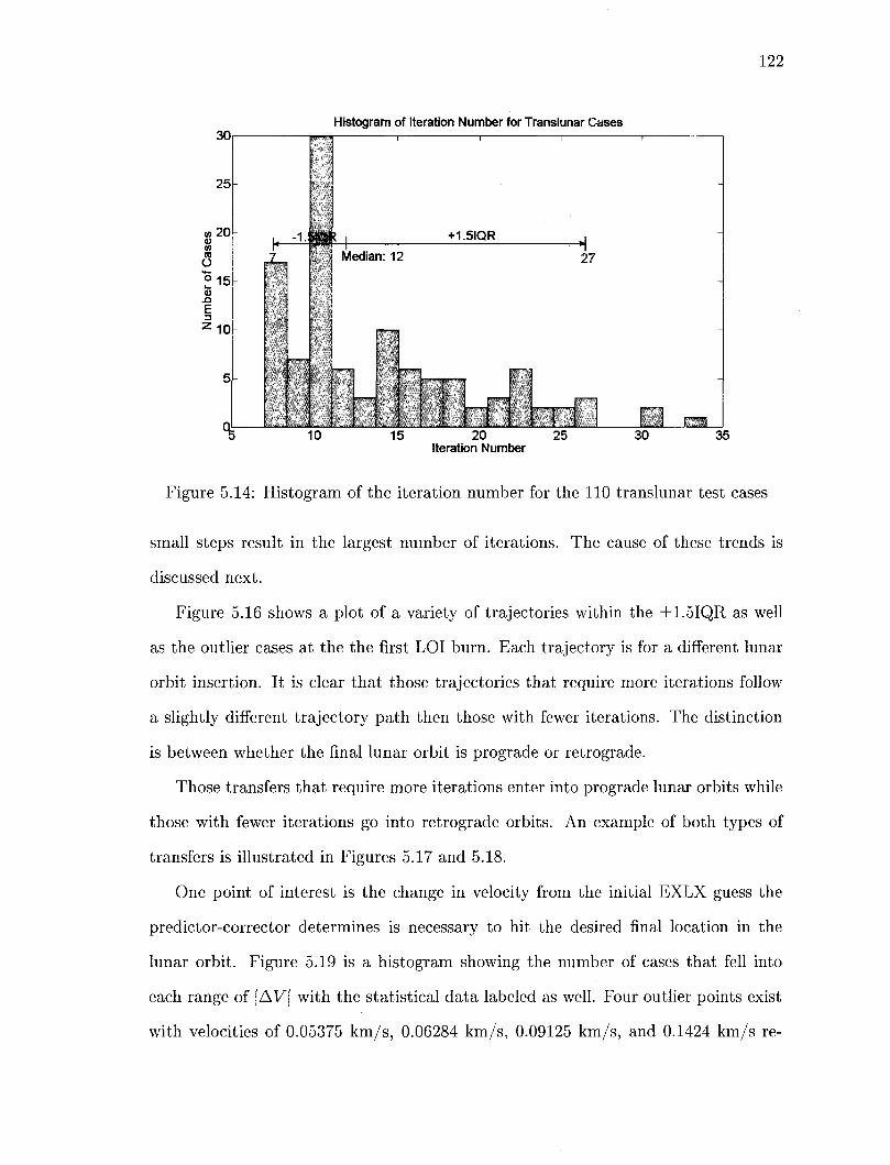
122

30,

25

co 2 0 01 (0 flj

O

Histogram of Iteration Number for Translunar Cases

15 v E

10

lafe +1.5IQR

Median: 12 27

p«fM)W

10 15 20 Iteration Number

25 30 35

Figure 5.14: Histogram of the iteration number for the 110 translunar test cases

small steps result in the largest number of iterations. The cause of these trends is

discussed next.

Figure 5.16 shows a plot of a variety of trajectories within the ±1.5IQR as well

as the outlier cases at the the first LOI burn. Each trajectory is for a different lunar

orbit insertion. It is clear that those trajectories that require more iterations follow

a slightly different trajectory path then those with fewer iterations. The distinction

is between whether the final lunar orbit is prograde or retrograde.

Those transfers that require more iterations enter into prograde lunar orbits while

those with fewer iterations go into retrograde orbits. An example of both types of

transfers is illustrated in Figures 5.17 and 5.18.

One point of interest is the change in velocity from the initial EXLX guess the

predictor-corrector determines is necessary to hit the desired final location in the

lunar orbit. Figure 5.19 is a histogram showing the number of cases that fell into

each range of |AV| with the statistical data labeled as well. Four outlier points exist

with velocities of 0.05375 km/s, 0.06284 km/s, 0.09125 km/s, and 0.1424 km/s re-

123

10°

10'

i<r

E1° E" ^-10 2

10

10

10

. Iteration Convergence Based on |AR| for Translunar Trajectories to include Outlier Cases

10 15 20 Iteration Number

25 30 35

Figure 5.15: Convergence rate for a range of translunar cases with iteration numbers within 1.5IQR as well as the rate for the three outlier cases

Transiunar Transfer Trajectories at LOI for a Variety of Test Cases

105

100

E

—-1.5IQR = 7 iterations —25% = 10 iterations —50% = 12 iterations

75% = 17 iterations —+1.5IQR = 27 iterations ,- _ outlier = 30 iterations —-outlier = 31 iterations —outlier = 34 iterations —Moon Trajactory

370 375 380 X (kkm)

385 390

Figure 5.16: Translunar trajectories at LOU for a variety of test cases

124

Translunar Transfer Trajectory for Prograde Lunar Orbit

1 7 0 -

160-

150-

140-

130-J t l 20 ->-

110-

100-

90-

80-

310 320 330 340 350 360 370 380 390 400 X (kkm)

v \;rur ••.'.-.:torir;r. li !r,c •

Figure 5.17: Example of a translunar transfer into a lunar prograde orbit (Test Case #77) ,

spectively. To determine if there is a correlation between the lunar orbit inclination

and the AV change required, the information from Figure 5.19 is separated by incli

nation and plotted as a stem plot in Figure 5.20. As with cases that require more

iterations, cases with prograde lunar orbits are more likely to require a larger change

in velocity from the initial EXLX guess. This is highlighted in Figure 5.20 where the

two dotted horizontal lines represent the cutoff points for the 50th percentile and the

75th percentile of the data respectively. All four outlier cases have prograde lunar

orbits as well.

5.4.1 Translunar Shooting Method Sensitivity

The translunar cases are tested in a similar manner to the STM in Section 4.4. An

initial perturbation is "applied one at a time to the radial1, tangential, and normal

components of the position and velocity vector to determine.rthe effects on the shoot-

LOI2

\

;A - • • • LQI1

125

Translunar Transfer Trajectory for Retrograde Lunar Orbit

170

160

150

140

J130-

120-

110-

100-

90

80-

! r ( i i

* - ! : -\

- !

- 4 - * ^ " i i i i

I

LOI3

\..i

^ \ ; \ -•

\

!LOI2

i

I

\.:..

\

;

I

\ \:

\ \-\ \

,

i

0LOI1

\ \

\ i

i

•

} -

; -310 320 330 340 350 360 370 380 390 400

X(kkm)

Figure 5.18: Example of a translunar transfer into a lunar retrograde orbit (Test Case #71)

30

25

20 (0 0) II) (0 O

2 15 a> .o E

10

Histogram of the Change in |AV| From EXLX Initial Guess for Translunar Test Cases

0.002613 krn/s

M.5IQR

0.04251 km/s

Median: 0.01628 km/s

_n_EL n HI 0.02 0.04 0.06 0.08 0.1 0.12 0.14 0.16

|AV| (km/s)

Figure 5.19: Histogram of the change in |AV| required for the translunar test cases

126

Change in Transfer Velocity From EXLX Initial Guess Based on Final Lunar Inclination

0.16r

0.14-

0.12-

0.1-

£.0.08-

>" <j.

0.06-

0.04-

0.02'|

J 0 50 9Q00 150 200 250 270 300 350

Inclination (deg) Figure 5.20: Stem plot of |AV| based on the final lunar orbit inclination

ing method convergence. The purpose is to obtain a grasp of the sensitivity of the

prediction-correction process to the initial guess. For Earth to Moon transfers one

expects the sensitivities to be high because the region of "linearity" for the trajectory

is correspondingly small. By adding perturbations, the ability of the state transition

matrix to represent the transfer trajectory is tested.

The perturbation percentages range from 0-4% and are tested on all 110 cases.

The results for the position perturbations are shown in Figure 5.21 and the results

for the velocity perturbations are shown in Figure 5.22. For illustrative purposes a

red dotted line is plotted to mark the cut off point of 40 iterations. Any data plotted

above this line failed to converge under the maximum nurriber of iterations. Note that

a convergence failure represents the need for a more accurate initial guess, in this case,

one that falls within the linear region assumed by the state transition matrix.

The first three columns of both plots highlight the convergence of all test cases with

zero perturbation. Increasing the perturbation error to 0.001%, plotted as the second

H i i I I i i i r

-Retrograde-

I !

» f l

kji k IT I i I

75% 50%

1

127

Iteration Number Based on Initial Position Perturbation for Translunar Cases

40

35

30 b. o>

_a

E

I25

c .2 1 2 0

15

10

T 1 1 1 1 1 1 1 r—i 1 1 r n i r

Convetgvnca Threshold

i i i

l l l l l l srR SrT 6rN SrR s'rT srN SrR 8rT 8rN SrR 6rT 8rN 8rR SrT 5rN irR SrT s'rN 5rR 8r? 5rN 8rR 5rT 8rN

0.001% 0.01% 0.1% 1% 2%

Initial Perturbation Percentage 3% 4%

Figure 5.21: Number of iterations based on initial position perturbation percentage for the translunar test cases

set of three columns, results in a few non-converging solutions, however majority

converge under 40 iterations. As the perturbation percentage increases, the number

of cases failing to converge increases as well. Errors in the radial direction of the

position perturbation plots and tangential direction of the velocity perturbation plots

result in far more non-converging solutions due to the direction of motion. With a

4% error in the initial radial direction of the position perturbation or 2% error in the

initial tangential direction of the velocity perturbation all but a few outlier cases fail.

Further work is conducted on the test cases that result in non-convergent solutions

after a certain perturbation to determine if a particular value or range of values for

individual parameters produce these results. Observations show that the inclination

of the final lunar orbit has the largest effect on whether or not a test case produces

a non-convergent solution for initial perturbations between 0.001%-4%. Figure 5.23

128

Iteration Number Based on Initial Velocity Perturbation Percentage for Translunar Cases

40

35

30

x> E = 25 c g

1 2 0

fconw«rg«fK# Threshold _

15

10

5h

n 1 1 1 1 1 1 r

1 1 1 1 1 1 1 1 1 SVR 5VT 5VN SVR SVT SVN 5VR 8VT 8VN 8VR SvT 8VN 8VR 8VT SvN 8VR SvT SvN 8VR SVT 8VN 8VR 8VT 8vN

0% 0.001% 0.01% 0.1% 1% 2% 3% 4%

Initial Perturbation Percentage

Figure 5.22: Number of iterations based on initial velocity perturbation percentage for the translunar test cases

provides a closer examination of the lunar orbit inclinations in question. The figure

shows a tendency for lunar orbits with low prograde inclinations, particularly those

between ±30 degrees, to have the most difficulty in converging when a perturbation

of 0.001% is added. As the perturbation increases, the range of lunar inclinations

that result in failing cases increases as well. Eventually, a perturbation of 3% ensures

all cases fail. Having already shown that prograde orbits require more iterations, it

makes sense that these same orbits would be more likely to fail if perturbations were

added further increasing the iteration number. However, what is interesting is that

adding very small perturbations, such as 0.001%, only affects the small inclinations.

Of the 24 cases that fail with a perturbation of 0.001% in the initial velocity, 21 of

the cases have inclinations less then 28°. A possible explanation for the sensitivity of

these particular orbits is the effect of the Moon's gravity potential.

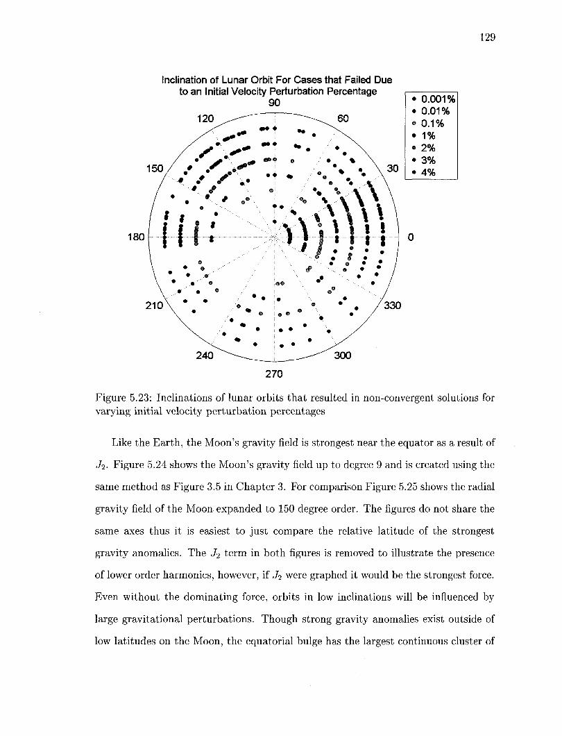
129

Inclination of Lunar Orbit For Cases that Failed Due

Figure 5.23: Inclinations of lunar orbits that resulted in non-convergent solutions for varying initial velocity perturbation percentages

Like the Earth, the Moon's gravity field is strongest near the equator as a result of

J2. Figure 5.24 shows the Moon's gravity field up to degree 9 and is created using the

same method as Figure 3.5 in Chapter 3. For comparison Figure 5.25 shows the radial

gravity field of the Moon expanded to 150 degree order. The figures do not share the

same axes thus it is easiest to just compare the relative latitude of the strongest

gravity anomalies. The J2 term in both figures is removed to illustrate the presence

of lower order harmonics, however, if J2 were graphed it would be the strongest force.

Even without the dominating force, orbits in low inclinations will be influenced by

large gravitational perturbations. Though strong gravity anomalies exist outside of

low latitudes on the Moon, the equatorial bulge has the largest continuous cluster of

130

anomalies. Thus, low inclination orbits that spend the majority of the time over the

equator will perturb more then higher inclined orbits. Since the gravity model for

EXLX only includes low order gravity coefficients its predicted trajectories will not

take into account the anomalies shown in Figure 5.24. The trajectories propagated

with the Cowell propagator, however, include the gravity model up to degree 9 and

thus will reflect all the anomalies seen in Figure 5.24.

Contour Plot of the Radial Component of the Acceleration Due to High Order Lunar Gravity (m/s ) up to Degree 9 Excluding J

150 200 250 Longitude, X (deg)

Figure 5.24: Radial component of the gravitational perturbation, aj3_9 ( ^ ) , due to lunar higher order gravity up to degree 9 excluding J2 with respect to latitude/longitude

For situations in which the EXLX trajectory flew through a large gravitational

anomaly and the Cowell propagator flew around, it would be difficult, if not impossible

to converge in most cases. This is the case with two of the outlier cases, Case #98 and

Case #99, with near equatorial final lunar orbits at i = 359° and i = 360° respectively.

Figure 5.26 and Figure 5.27 highlight the results of the shooting method at the first

LOI. The blue line on the plots represent the trajectory of the Moon and the red line

is the predicted trajectory output from EXLX. The green lines represent the multiple

131

-300 -200 -100 0 100 200 300

Radial Gravity Anomaly (mgals)

Figure 5.25: Radial gravity field (mGal) of the Moon expanded to degree 150 with the J2 term removed [51]

attempt trajectories the predictor-corrector tries until it converges within 1 x 10~6 km

of the desired final position. The axes are with respect to an Earth centered at (0,0)

coordinates. Observing the propagated trajectories near the path of the Moon, it is

clear the Cowell propagator is influenced by an acceleration which makes it difficult

to follow the predicted EXLX trajectory. In fact, despite both cases having initially

prograde final orbits, the converged solution at the first lunar orbit insertion burn

puts the vehicle on a retrograde path. This is possible because the shooting method

targets a final position vector and not a final velocity vector which would determine

the direction of the orbit and whether or not its motion is direct or retrograde.

Converged Translunar Trajectory at LOU for Outlier Case #98

105-

100

95

90

85

I I I

^ • - :1 H-3 - '

i I i

I

• - - V ,

9 \ \

! \. \ \

, \ \

—EXLX Trajactory —Moon Trajactory

Propag. Iterations

-

-

\ \ i I

370 375 380 X(kkm)

385 390

Figure 5.26: Convergence of translunar test Case #98 , i = 359°, at LOU with 31 iterations

Converged Translunar Trajectory at LOI for Outlier Case #99

100-

95

E

90

85

80

370 375

I

^

I

I

- -

i

I

\J

I

I —EXLX Trajactory —Moon Trajactory

Propag. Iterations

^^^^^^^K w : \

\

\ -

\ \ \ \

i > i

380 385 X(kkm)

390

Figure 5.27: Convergence of translunar test Case #99 , i = 360°, at LOU with 34 iterations

133

To test the theory that higher order gravity influences the large number of it

erations for both cases, 31 and 34 respectively, Case #98 and Case #99 are run

through the predictor-corrector again with only the lunar gravity coefficients utilized

by EXLX: J2-4 included. The results are seen Figure 5.28 and Figure 5.29. In both

cases the iteration number decreases drastically. For Case #98 the number decreases

from 31 to 20, for Case #99 from 34 to 18 iterations. The figures also illustrate that

removing the higher order lunar gravity coefficients alleviates the issue of the orbit

path switching from prograde to retrograde. The remainder of the test cases with

final lunar orbit inclinations less than 25° but greater than 335° were run through

the same test. A comparison of the iteration number statistics between these cases

with and without HOG applied is plotted in a histogram in Figure 5.30. The median

value of iterations drops from 18 to 16 with the range for the middle 50% of the data

dropping from between 14-22 iterations to between 13.25-18 iterations when HOG

is removed. Further, the ±1.5IQR decreases from 8-34 iterations to 8-21 iterations.

This information illustrates the contribution of high order gravity to the sensitivity

of the Cowell predictor-tool for final lunar orbits with low inclinations.

Converged Translunar Trajectory at LOU for Outlier Case #99 Higher Order Lunar Gravity Removed

105F

100

95

I >-

90

85

-EXLXTrajactory -Moon Trajactory Propag. Iterations

#

370 375 380 X(kkm)

385 390

Figure 5.28: Convergence of translunar test Case #98 , i = 359°, at LOU with 20 iterations after lunar higher order gravity is removed

105

100j

Converged Translunar Trajectory at LOU for Outlier Case #99 Higher Order Lunar Gravity Removed

I 95

90

85

EXLXTrajactory -Moon Trajactory Propag. Iterations

370 375 380 385 X(kkm)

390

Figure 5.29: Convergence of translunar test Case #99 , i = 360°, at LOU with 18 iterations after lunar higher order gravity is removed

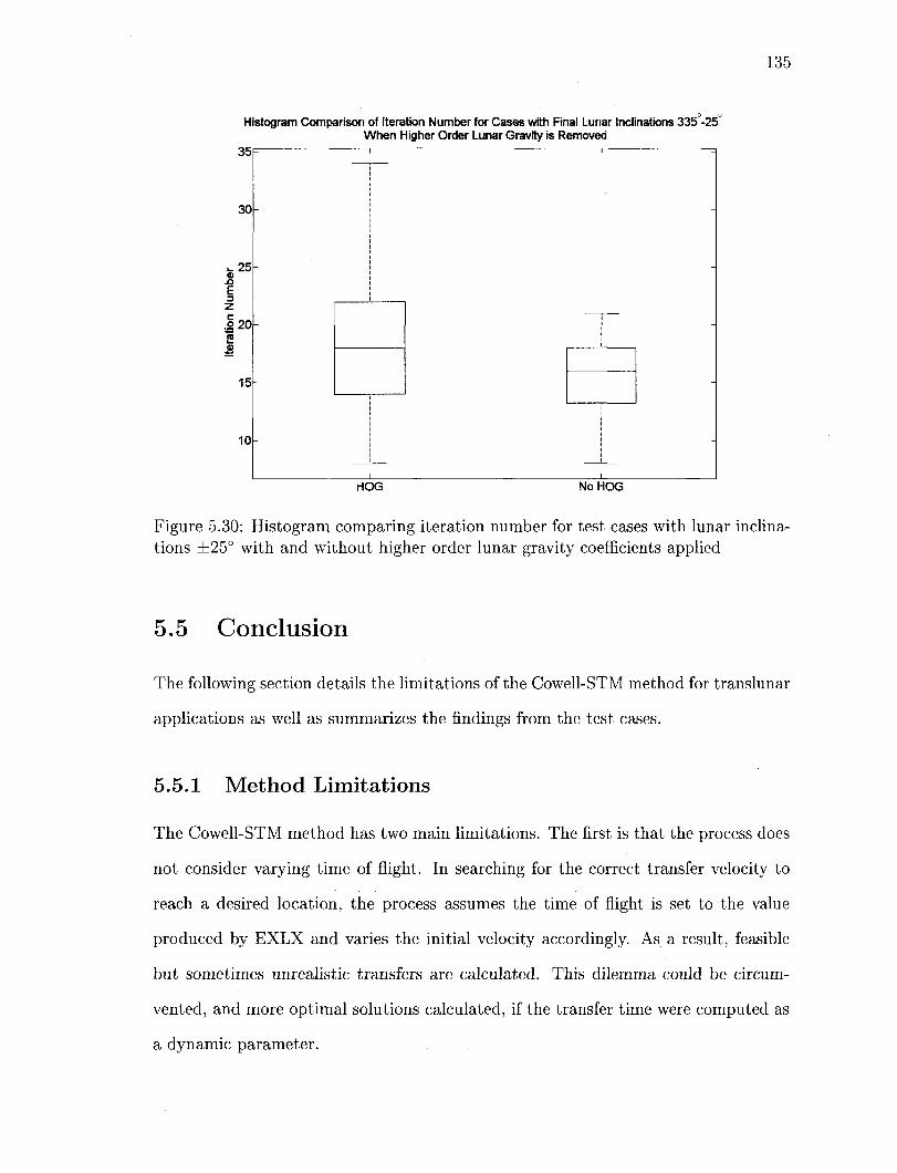
135

Histogram Comparison of Iteration Number for Cases with Final Lunar Inclinations 335 -25° When Higher Order Lunar Gravity is Removed

35 F 1 ' =

30- |

_ 2 5 - j

xi !

E : 3 ! ,

Z ^ ^ _

1 2 0 - I -jj) I ! .

15-1 0 - i I -

HOG No HOG

Figure 5.30: Histogram comparing iteration number for test cases with lunar inclinations ±25° with and without higher order lunar gravity coefficients applied

5.5 Conclusion

The following section details the limitations of the Cowell-STM method for translunar

applications as well as summarizes the findings from the test cases.

5.5.1 Method Limitations

The Cowell-STM method has two main limitations. The first is that the process does

not consider varying time of flight. In searching for the correct transfer velocity to

reach a desired location, the process assumes the time of flight is set to the value

produced by EXLX and varies the initial velocity accordingly. As a result, feasible

but sometimes unrealistic transfers are calculated. This dilemma could be circum

vented, and more optimal solutions calculated, if the transfer time were computed as

a dynamic parameter.

136

An additional limitation is that the predictor-corrector method only calculates

the transfer velocity for the first LOI burn even though all the transfers tested were

three burn maneuvers. In an ideal situation the method would determine the transfer

velocity needed for the first burn and using the Cowell propagator compute the final

states at LOU. The states at LOU then become the initial conditions to determine

the transfer velocity needed to reach LOI2 as predicted by the EXLX multi-conic

propagator. This process would continue through LOI3 putting the vehicle in its

final lunar orbit. The difficulty in such a method is that any change required in one

burn's initial conditions would cause a chain reaction changing the initial conditions

of any previous burns. For example, consider the situation in which the TLI transfer

velocity to reach LOU is calculated and the states are propagated forward in time.

From here a second shooting method calculates the transfer velocity from LOU to

LOI2. However, if the "shoot out" between LOU and LOI2 does not place the final

position at LOI2 within tolerance, the initial velocity for the LOU transfer must be

updated. Back propagating the change in velocity from LOU to TLI results in a

different position and initial velocity. Since the position at TLI cannot change this

will require an additional "shoot out" between TLI and LOU. This iterative process

of dealing with more than one transfer burn is known as two-level targeting. One way

to alleviate some of the obstacles faced with the complexity of multi-level targeting

is to allow the time of flight to vary from the values determined by EXLX. Both

the time constraint and multi-level targeting process should be considered for future

updates on the Cowell-STM predictor-corrector method.

5.5.2 Summary of Test Results

Updating the initial transfer velocity produced by the EXLX multi-conic propagator

with the Cowell-STM method identifies a number of sensitivities in the test case se

lection. Here "sensitivities" are defined as cases that result in a larger than average

137

number of iterations to converge. The first is the sensitivity of the process to trans

fers entering into lunar orbits with low inclinations. For many of these cases, low

lunar inclinations lead to converged trajectories with retrograde orbits. Inherently,

retrograde orbits are not more difficult to transfer into then prograde orbits, hence

the sensitivity is linked to the perturbation that causes the transfer to switch from

a prograde to retrograde orbit. As is shown, higher order gravity coefficients in the

Cowell model result in perturbations close to the Moon that are not predicted by

the EXLX multi-conic propagator. As a result, certain trajectories become difficult

to follow as the Moon's gravitational pull affects the vehicle motion. In some cases,

the converged solution has to switch from a prograde to retrograde orbit in order to

meet the final position tolerance. Cases that require a switch in orbit type from the

initial guess require a larger iteration number. The removal of higher order gravity

from the Cowell method alleviates the high iteration number problem. An additional

improvement to the predictor-corrector method to help reduce this sensitivity would

be to include some of the lunar low order gravity partials in the state transition ma

trix. The closer the STM mirrors the Cowell propagator in terms of perturbation

models, the less deviation between the two methods and the fewer iterations needed

for convergence.

The initial perturbation percentage test illustrates that by perturbing the initial

guess provided by EXLX by only 4%, all translunar test cases fail to converge. The

fact that such a small perturbation could result in complete failure illustrates how

sensitive the predictor-corrector is to the initial guess.

Having tested and validated the performance of the Cowell-STM tool in translunar

conditions, the functionality of the predictor-corrector is substantiated by testing low

Earth orbit transfer situations.

Chapter 6

Low Earth Orbit Application

The higher order propagator is tested on low Earth orbit applications by utilizing the

Cowell-STM predictor-corrector method to determine the appropriate delta velocities

to transfer from one LEO orbit to another. These cases differ from the translunar

cases in two major aspects. The first is the lack of a robust program such as EXLX

to predict initial transfer velocities and flight times. The second is the much stronger

influence of drag on the vehicle's motion. Chapter 6 begins with a discussion of

Lambert's problem and the use of its solution as an initial guess for the transfer

velocity between two low Earth orbits. Section 6.2 details the test case selection

process, and the final section discusses the performance of the predictor-corrector

process as applied to LEO scenarios.

6.1 Lambert's Method

Lambert's method forms the basis of the prediction algorithm for low Earth orbit

problems. It is an orbit determination technique that given two position vectors and

the time of flight, calculates the unknown transfer orbit [22][23],

[vi, v2] = lambert (r1; r2, At). (6.1)

138

139

Battin derives a formulation for the Lambert problem combining Lagrange's equations

from his proof of Lambert's theorem and Gauss's equations from the Theoria Motus

i •

6.1.1 Lagrange's Equations

Lagrange's form of the transfer-time equation for elliptical orbits is

3

y/Jifa — ti) = a5 [(a — sin a) — ()3 — sin/3)], (6.2)

with a = (j) + tp and (3 = 4> — ip. The variables <f> and ip are defined with respect to

the eccentric anomalies of the two orbits, E\ and E2, by the equations

cos <f> = e cos \ (E2 - Ei) , (6-3)

and

iP = 1 (E2 - Ex). (6.4)

For fixed geometry, Lagrange's transfer-time equation is a function only of the semi-

major axis. However, this poses a problem in that the transfer time is a double-valued

function of a: each pair of conjugate orbits has the same semimajor axis and the

derivative of the transfer time with respect to a is infinite for that value of a = am.

Here am is the semimajor axis of the minimum energy orbit. Thus for convenience

Equation 6.2 is recast in the form

r ^ ~ u +^ a-sina 3 /3-s in/5 \Hr(t2 -ti) = . . 3 , A , „ . , (6.5)

where

\=(tz£)\ (6.6)

140

and c is the chord such that

c = 2a sin ip sin <ft, (6.7)

with

\s = a (cos ip — cos <f>). (6.8)

A similar transformation for hyperbolic orbits (see Reference [7] for details of the

transformation process) exists, specifically

/ u , . sinh a — a , o sinh B — B , AJ^(t2-t1) = on A3 tTTJ~- (6-9 V «m sinh3 ±a sinh31/5 V '

By defining the hypergeometric function Qa as

gQ = <( ^ F (6-10) sinh a—a sinh3^o:

for elliptic orbits, Equations 6.5 and 6.9 become identical. Thus,

Y (*2 - h) = Qa- A3Q/3 (6.11)

where<5Q is a hypergeometric function such that:

Q*={ 3 V 2 4 ^ • (6.12) | F ( 3 , l ; | ; - s i n h 2 | a )

Here the notation refers to that of hypergeometric series:

, a(a+l)(q+2)/3(/M-l)(/3+2) ^3 (6.13)

7 ( 7 + l ) ( 7 + 2 ) 3!

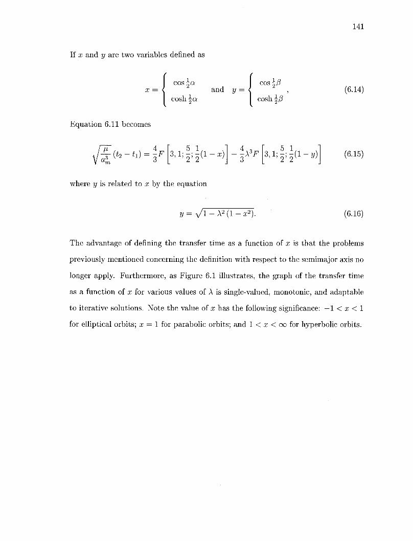
141

If x and y are two variables defined as

x = cos ^a

cosh \ a and y =

cos \{5

cosh \{5 (6.14)

Equation 6.11 becomes

^ (*2 - *i) = ~,F 3,1; | ; | ( 1 - x) -A3F 5 1,

3 , l i 5 i 5 ( l - » ) (6.15)

where ?/ is related to x by the equation

y = ^l-\2(l-x2). (6.16)

The advantage of defining the transfer time as a function of x is that the problems

previously mentioned concerning the definition with respect to the semimajor axis no

longer apply. Furthermore, as Figure 6.1 illustrates, the graph of the transfer time

as a function of x for various values of A is single-valued, monotonic, and adaptable

to iterative solutions. Note the value of x has the following significance: — 1 < x < 1

for elliptical orbits; x = 1 for parabolic orbits; and 1 < x < oo for hyperbolic orbits.

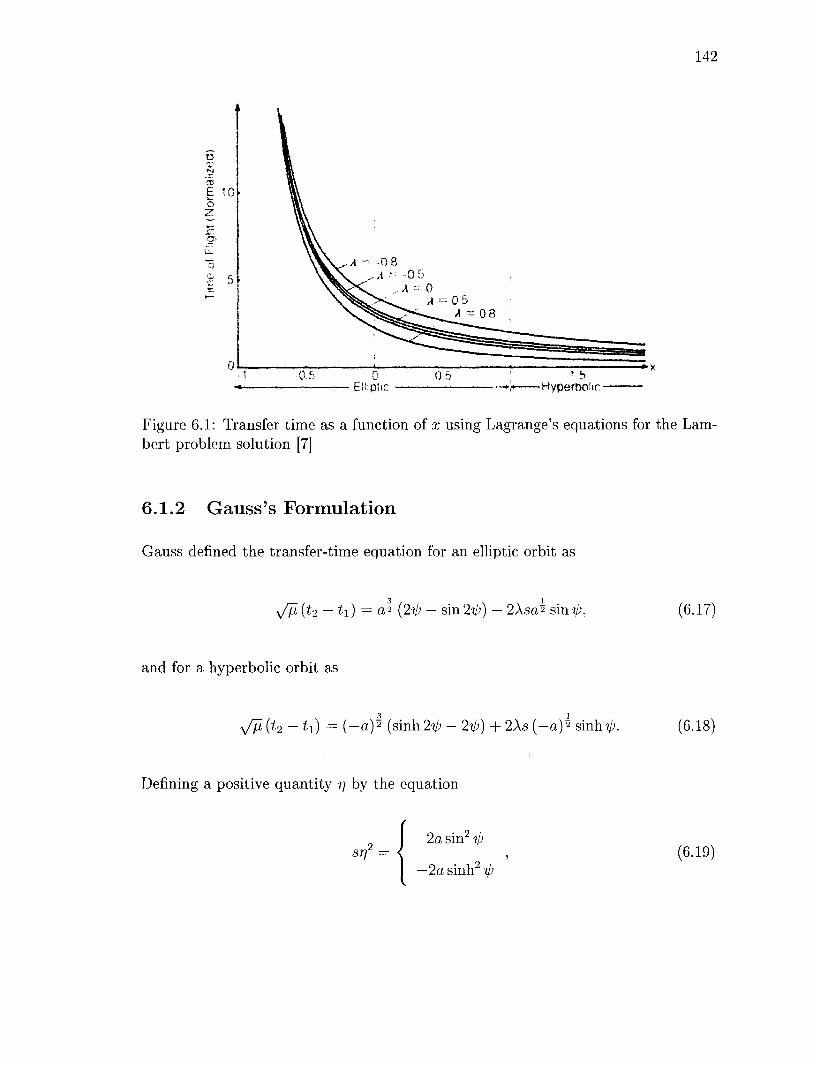
142

fl5

£ 10 o Z

Elliptic 05 1.5

" • X

~*t Hyperbolic-

Figure 6.1: Transfer time as a function of x using Lagrange's equations for the Lambert problem solution [7]

6.1.2 Gauss's Formulation

Gauss denned the transfer-time equation for an elliptic orbit as

\/7^(*2 — h) = «2 (2^ — sin2^) + 2Asa2 smi/>, (6.17)

and for a hyperbolic orbit as

V7*(*2 — *i) = ( - a ) 2 (sinh2^-2?/;) + 2As(-a)2sinhV'. (6.18)

Defining a positive quantity r/ by the equation

9 ST) =

2 a sin2 ip

—2a smh2 ip (6.19)

143

the transfer-time equation is rewritten in the form

,JY (t2 - ii) = v'Qw + 4XV. (6.20)

With additional transformations

• M d-*)2+«*»'§* , (6.21) ( l - A ) 2 - 4 A s i n h 2 ± V

and the hyperbolic function, one can write

Introducing the symbol

, | F ( 3 , l ; f ; s i n 2 ^ ) Q^={ 3 V 2 2 ' • (6.22)

§ F ( 3 , l ; f ; - s i n h 2 ± V )

sin2 \ii Si={ 2 , (6.23)

- sinh2 T;I/J

Equation 6.20 can be rewritten as

A / 4 (*2 - *i) = ^ f 3,1; | ; 5 ^ + 4AT/, (6.24)

where

r?2 = (1 - A)2 + 4AS! T? > 0 (6.25)

and 0 < S\ < 1 for elliptical orbits; Si = 0 for parabolic orbits; and —oo < Si < 0

hyperbolic orbits.

Figure 6.2 is a graph of the transfer time as a function of —Si for various values of

A. Like Figure 6.1, the curves are monotonic but they are not conducive to iterative

solutions as evident in the crossing curves.

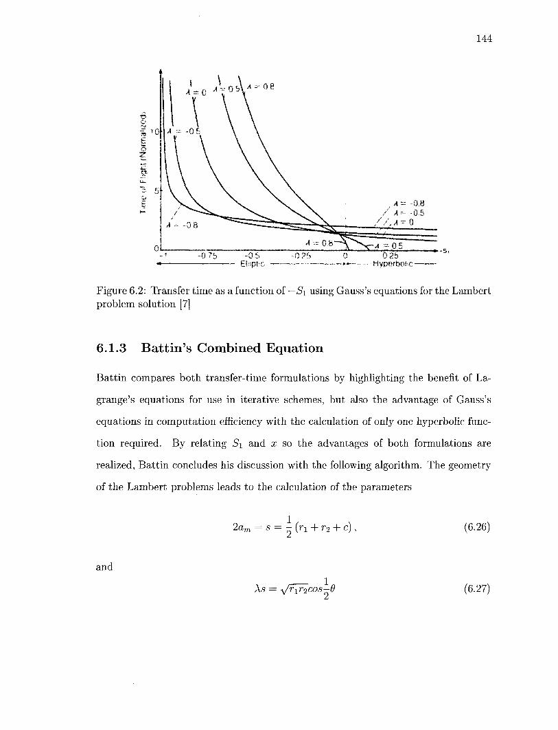
144

Figure 6.2: Transfer time as a function of —Si using Gauss's equations for the Lambert problem solution [7]

6.1.3 Battin's Combined Equation

Battin compares both transfer-time formulations by highlighting the benefit of La

grange's equations for use in iterative schemes, but also the advantage of Gauss's

equations in computation efficiency with the calculation of only one hyperbolic func

tion required. By relating Si and x so the advantages of both formulations are

realized, Battin concludes his discussion with the following algorithm. The geometry

of the Lambert problems leads to the calculation of the parameters

2am = s = - (n + r2 + c), (6.26)

and

As = yjrir2cos-0 (6.27)

145

where c is the chord length between the two magnitude position vectors T\ and r2,

c = yjr\ + r\ - 2r1r2 cos{6) (6.28)

and 9 is the transfer angle between the two position vectors. With an initial guess

for defined in Lagrange's formulation, the following,

and

y=y/l-X>(l-x*),

r) = y-\x, (6.29)

Si = \ (1 - A - xrj),

Q = ^ 3 , 1 ; ! S i ) ( 6- 3 0 )

are computed where F (3,1; | ; ^i) is a hypergeometric function which may be evalu

ated by continued fractions. These values are utilized to find the transfer time from

3 ( * 2 - t i ) = 7/3Q + 4A77. (6.31)

The algorithm is iterated upon using Newton's method (see Reference [7]) until a

desired convergence is acquired. The velocity vector at the initial position in terms

of the value x found is

2\^-(X + xV) in + JTf sin ^9ih xin}, (6.32)

where i n is the unit vector in the direction of ri and i^ is the unit vector normal to

the orbital plane. Figure 6.3 summarizes the Lambert 2-body dynamic formulation in

an algorithm flow chart. The output of the formulation is used as the initial transfer

velocity guess for low Earth orbit calculations.

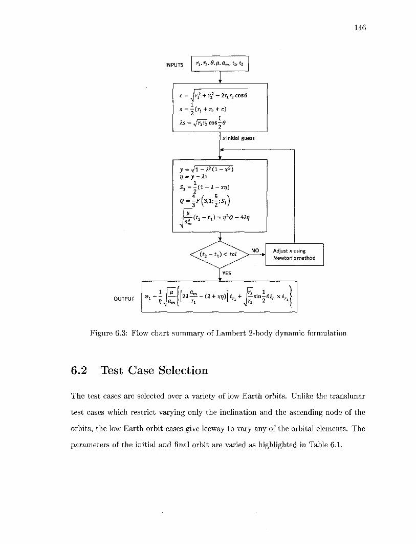
146

INPUTS r1,r2,0./*,am#t1,tj

c = jr^ + r^ — 27^2 cosfl

1

. 1 As = J n r , cos - e v i 2

x initial guess

y=Vl-A2(l-x2) »7 = y-Ax

OUTPUT

Adjust x using Newton's method

i [/* Ir ,0™ ,„ j In i

Figure 6.3: Flow chart summary of Lambert 2-body dynamic formulation

6.2 Test Case Selection

The test cases are selected over a variety of low Earth orbits. Unlike the translunar

test cases which restrict varying only the inclination and the ascending node of the

orbits, the low Earth orbit cases give leeway to vary any of the orbital elements. The

parameters of the initial and final orbit are varied as highlighted in Table 6.1.

147

Parameter altitude

e i Q

u V

Initial Orbit 100 km

0-0.9 0° - 90°

0° 0°

135° - 225°

Final Orbit 300-500 km

0-0.9 0° - 90°

0° 0° 0°

Table 6.1: Variation in initial and final orbit parameters for testing LEO cases

Realistically, low Earth orbit transfers occur between similar orbits with differing

altitudes and phasing angles. As a result, no cases with drastically different initial

and final orbits, such as a transfer between a polar and equatorial orbit, are tested.

Transfers such as these are also not tested because they are prohibitively expensive

to achieve with a single burn and only 2-burn sequences were tested in this thesis.

Instead, the altitude of the initial orbit is set at 100 km with the final altitude

varying as defined in Table 6.1. The eccentricities and inclinations of both orbits

are set equal. The right ascension of the ascending node is set to 0° for both orbits

and the true anomaly of the initial orbit is varied to ensure a realistic transfer angle.

The true anomaly angle is varied ±45° off the basic Hohmann transfer angle of 180°.

Preliminary testing highlights a convergence issue with transfer angles of exactly 180°,

thus angles of 180° ±2 but never exactly 180° are tested. A discussion of this limitation

is in Section 6.4.1. The two-body Lambert formulation as discussed in Section 6.1.1 is

used to calculate the initial delta velocity. Examples of the low Earth initial and final

orbits for a variety of inclinations and eccentricities tested are illustrated in Figure

6.4. Figure 6.5 depicts a range of transfer angles tested as well.

Lambert calculations require orbit transfer times and though determining the

time of flight (TOF) is not central to this research, a feasible value is required to

test low Earth orbit cases. The time of flight is found using a rudimentary guess

and check iterative procedure. The time of flight is initially set to a number with

a large enough value so to provide enough time to transfer between the two orbits,

148

Example of Tested LEO Orbits Over a Variety of Eccentricities and Inclinations

x10 4

3 -

2 -

1-

l o -N

-1

-2

-3H

-4

x10

— Initial Orbit — Final Orbit

x10

X(km) Y(km)

Figure 6.4: Example of low Earth initial and final orbits for a variety of eccentricities and inclinations

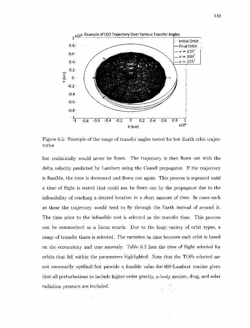
149

X104 Example of LEO Trajectory Over Various Transfer Angles

0.8^

0.6r

0.4

_ 0.2| E ^ Or >

-0.2J-

-0.4

-0.6L

-0.8(-

Initial Orbit -Final Orbit -v = 135° -v = 180° -v = 255°

-1 -0.8 -0.6 -0.4 -0.2 0

X(km)

0.2 0.4 0.6 0.8 1 xlO4

Figure 6.5: Example of the range of transfer angles tested for low Earth orbit trajectories

but realistically would never be flown. The trajectory is then flown out with the

delta velocity predicted by Lambert using the Cowell propagator. If the trajectory

is feasible, the time is decreased and flown out again. This process is repeated until

a time of flight is tested that could not be flown out by the propagator due to the

infeasibility of reaching a desired location in a short amount of time. In cases such

as these the trajectory would tend to fly through the Earth instead of around it.

The time prior to the infeasible test is selected as the transfer time. This process

can be summarized as a linear search. Due to the large variety of orbit types, a

range of transfer times is selected. The variation in time between each orbit is based

on the eccentricity and true anomaly. Table 6.2 lists the time of flight selected for

orbits that fell within the parameters highlighted. Note that the TOFs selected are

not necessarily optimal'but provide a feasible value for-tfie^Lambert routine given

that all perturbations to include higher order gravity, n-body motion, drag, and solar

radiation pressure are included.

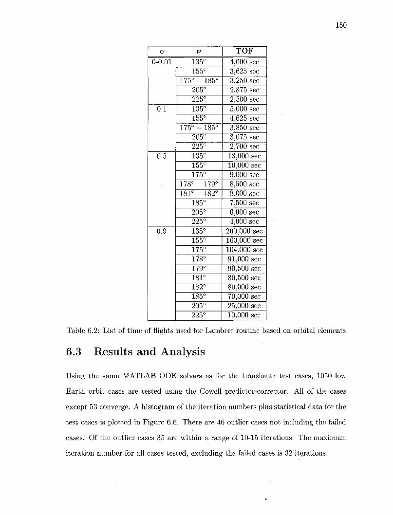
e

0-0.01

0.1

0.5

0.9

V

135° 155°

175° - 185° 205° 225° 135° 155°

175° - 185° 205° 225° 135° 155° 175°

178° - 179° 181° - 182°

185° 205° 225° 135° 155° 175° 178° 179° 181° 182° 185° 205° 225°

TOF 4,000 sec 3,625 sec 3,250 sec 2,875 sec 2,500 sec 5,000 sec 4,625 sec 3,850 sec 3,075 sec 2,700 sec 13,000 sec 10,000 sec 9,000 sec 8,500 sec 8,000 sec 7,500 sec 6,000 sec 4,000 sec

200,000 sec 160,000 sec 104,000 sec 91,000 sec 90,500 sec 80,500 sec 80,000 sec 70,000 sec 25,000 sec 10,000 sec

Table 6.2: List of time of flights used for Lambert routine based on orbital elements

6.3 Results and Analysis

Using the same MATLAB ODE solvers as for the translunar test cases, 1050 low

Earth orbit cases are tested using the Cowell predictor-corrector. All of the cases

except 53 converge. A histogram of the iteration numbers plus statistical data for the

test cases is plotted in Figure 6.6. There are 46 outlier cases not including the failed

cases. Of the outlier cases 35 are within a range of 10-15 iterations. The maximum

iteration number for all cases tested, excluding the failed cases is 32 iterations.

151

Histogram of Iteration Number for LEO Cases 500 —

450

400

350

$300 en O °250 <B

§200 z

150

100

50

°0 5 10 15 20 25 30 35 40 45 Iteration Number

Figure 6.6: Histogram of the iteration number for the 1050 low Earth orbit test cases

The convergence trend of a number of the cases as well as the range of outlier cases

is highlighted in Figure 6.7. Similar to the trend seen with the translunar convergence

rates, those cases that require more iterations were a result of early oscillating values

of \AR\ or iterative procedures that took multiple very small tests. For example,

the oscillating case requiring 22 iterations began with a |Ai?| of 44 km on the first

attempt but on the second iteration produced a |Ai?| of 327 km. The oscillations

continued for 17 iterations until the magnitude of the position vector became small

enough for the STM corrector to calculate a velocity that would put the final position

vector in a much closer range to the desired location. Likewise, the case that has the

largest number of iterations outside of failing cases at 32, drops to below 1 km after 4

iterations but then proceeds to take 28 very small steps until it converges. The cases

that produce these difficult convergence trends are analyzed next.

To determine which test case parameters have the greatest effect on producing

1.5KR*1 5K3R

-k W

10 Median: 6

152

Iteration Convergence Based on |AR| for LEO Trajectories to include Outlier Cases 10

102

10°

~10-2

E S"

^ - l o " 4

10"6

10"8

10"1<

0 5 10 15 20 25 30 35 Iteration Number

Figure 6.7: Convergence rate for a range of LEO cases with iteration numbers within 1.5IQR as well as the range of the outlier cases

outlier and failing solutions, histograms of individual parameter data are plotted.

The results are found in Figures 6.8-6.11. Figure 6.8 illustrates no correlation between

iteration number and altitude in that an almost equal number of all three altitudes

tested fall into the outlier and failing category. In looking at the effects of eccentricity,

Figure 6.9 highlights that cases with the largest eccentricity of 0.9, produce the most

outlier and failing cases. This seems to be a result of the large transfer time. As

the error in the state transition matrix increases over time it becomes more difficult

to accurately update the velocity on each "shoot out" attempt resulting in more

iterations. From Figure 6.10, the ease in which equatorial and polar orbits quickly

converge is highlighted. From the 150 cases tested for each inclination, only 7 cases

with an inclination of 0° and 4 cases with an inclination of 90° result in outlier or

failing cases. This is because orbits with motion in only two planes tend to stay

in those planes during convergence attempts, thus reducing the complexity of the

±1.5IQR Outliers

-3 Iterations -5 Iterations -6 Iterations 8 Iterations 9 Iterations 10 Iterations 11 Iterations 12 Iterations

-15 Iterations 17 iterations

-19 Iterations -21 Iterations -22 Iterations -32 Iterations

Convergence Tolerance

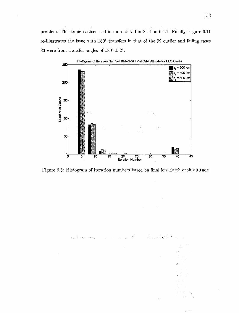
153

problem. This topic is discussed in more detail in Section 6.4.1. Finally, Figure 6.11

re-illustrates the issue with 180° transfers in that of the 99 outlier and failing cases

83 were from transfer angles of 180° ± 2°.

250

200

Histogram of Iteration Number Based on Final Orbit Altitude for LEO Cases

u m O

ilOO

50

_tfb_ 10 15 20 25

Iteration Number 30

•v Hv Ov

= 300 km

= 400 km

= 500 km

35 40 45

Figure 6.8: Histogram of iteration numbers based on final low Earth orbit altitude

Histogram of Iteration Number Based on Final Orbit Eccentricity for LEO Cases 200

180

160

140

IB

8120 8 • I —

2ioo o> .Q

I 80 z

60

40

20

n

I

« 1 • 1

L i i °0 5

i i

i

i •i

" %

l i tr-ii... 10 15

i i i i

1 _,__ , , 1 20 25 30 35

Iteration Number

i

• e = 0 • e = 0.01 • e = 0.1 H e = 0.5 H e = 0.9 "

-

-

-

_

r

y 40 4

Figure 6.9: Histogram of iteration numbers based on initial/final low Earth orbit eccentricity

120

100

Histogram of Iteration Number Based on Final Orbit Inclination for LEO Cases

ro O

° 60

E 3

20 25 Iteration Number

Figure 6.10: Histogram of iteration numbers based on initial/final low Earth orbit inclinations

155

100r

90

80

70-

<n 2S 60f-ro O ° 50 <u i 40h z

Histogram of Iteration Number Based on Initial Orbit True Anomaly for LEO Cases

30-

20

10-

0-

I

1

-

-

I 1 1 1 1 1

| v 0 = 135°

• v o = 155° • v o = 175° Mv0=™ • v 0 = 179°

I

] &o = 181

lv0- i82°

l v 0 = 185°

• v0 = 2 0 5 ° l v 0 = 225°

U. I . . I • H i , i . • I I I

10 15 20 25 Iteration Number

30 35 40 45

Figure 6.11: Histogram of iteration numbers based on initial low Earth orbit true anomalies

As with the translunar test cases, a point of interest is the change in velocity from

the initial Lambert two-body guess the predictor-corrector determines is necessary to

hit the desired final location in low Earth orbit. Figure 5.19 is a histogram showing

the number of cases that fall into each range of | AV|. All cases that fail to converge

are given a velocity value of 1 km/s for plotting purposes. 156 outlier points exist

outside the 53 failing cases, which is over three times the number of outlier cases

produced when just looking at the iteration number. An interesting fact to note is

how much larger the |AV|s for the LEO cases are compared to the translunar cases.

This underscores the higher fidelity of EXLX as a transfer velocity predictor compared

to the Lambert routine for their respective transfer missions. This observation is not

a surprise since EXLX includes 4-body motion and J2-J4 gravity coefficients whereas

Lambert only assumes two-body motion with no perturbations.

In Figures 6.13-6.16 histograms illustrate the effect varying parameters have on

the change in velocity. Figure 6.13 shows there is no correlation between the change in

156

velocity and the final altitude in that all altitudes tested produce the relatively same

number of outliers. The trend in eccentricity changes in Figure 6.9 in that the three

smallest eccentricities result in the largest velocity change. This is due to the fact

that drag has the strongest effect at low altitudes which orbits with low eccentricities

will maintain the longest. Since the Lambert transfer velocity does not consider drag

in its calculations, a much stronger thrust is necessary to counter the perturbation.

In observing how inclination played a role in effecting the |AV| it is apparent that

the Lambert routine calculates the most accurate transfer velocities for equatorial

and polar orbits in that only 3 cases with an inclination of 0° and no cases with an

inclination of 90° produce outlier or failing results. Figure 6.16 reiterates the point

that transferring 180° is the most difficult transfer angle. All but one case with an

initial true anomaly of ±2° off a perfect Hohmann 180° transfer results in outlier or

failing cases.

Comparing Figures 6.8-6.16, it is seen that higher iteration numbers do not nec

essarily equate to higher delta velocities. For the 103 outlier velocity cases that do

not include failing cases only 20 have iteration numbers greater than 10. The case

with the highest number of iterations, 32, has only a velocity change requirement of

0.00409 km/s where one case that converges in 8 iterations has a velocity change of

0.6249 km/s. Thus orbits with high velocity changes do not necessarily indicate dif

ficult transfers for the Cowell predictor-corrector method. Instead, orbits with large

velocity changes are those that the Lambert routine has difficulty predicting accurate

initial transfer velocities for.

As with the translunar test cases, the low Earth orbit cases are tested over a

range of initial perturbation percentages to determine the sensitivity of the initial

guess. These results are plotted in Figure 6.17 for the,position perturbations and

Figure 6.18 for the velocity perturbations. For perturbations below 1% the position

and velocity perturbations results are very similar in that around the same number of

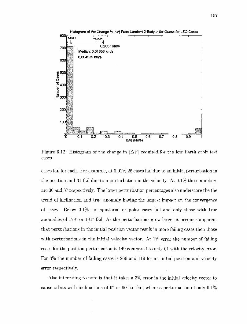
157

800

700

600

8500 in (0

O °400 o XI

E z 3 0 0

200

100

Histogram of the Change in |AV| From Lambert 2-Body Initial Guess for LEO Cases

•1.5IQR +1.5IQR

0.2837 km/s

Median: 0.01656 km/s

0.004529 km/s

Figure 6.12: Histogram of the change in |AV| required for the low Earth orbit test cases

cases fail for each. For example, at 0.01% 26 cases fail due to an initial perturbation in

the position and 31 fail due to a perturbation in the velocity. At 0.1% these numbers

are 30 and 37 respectively. The lower perturbation percentages also underscore the the

trend of inclination and true anomaly having the largest impact on the convergence

of cases. Below 0.1% no equatorial or polar cases fail and only those with true

anomalies of 179° or 181° fail. As the perturbations grow larger it becomes apparent

that perturbations in the initial position vector result in more failing cases then those

with perturbations in the initial velocity vector. At 1% error the number of failing

cases for the position perturbation is 149 compared to only 61 with the velocity error.

For 3% the number of failing cases is 266 and 119 for an initial position and velocity

error respectively.

Also interesting to note is that it takes a 3% error in the initial velocity vector to

cause orbits with inclinations of 0° or 90° to fail, where a perturbation of only 0.1%

Change in Transfer velocity From Lambert 2-Body Initial Guess Based on Final Orbit Altitude

50H

J a f = 300 km Q a f = 400 km

Q a f = 500km

0.1 0.2 BTI i WT\ i r n .

0.3 0.4 0.5 |AV| (km/s)

Figure 6.13: Histogram of LEO cases comparing change in transfer velocity from two-body Lambert initial guess based on final orbit altitude

Change in Transfer Velocity From Lambert 2-Body Initial Guess Based on Final Orbit Eccentricity 20X),

H e B e U e H e H e

= 0 = 0.01 = 0.1 = 0.5 = 0.9

M J LMJ L I ,_•_• i U H J iB-JJ 0.1 0.2 0.3 0.4 0.5 0.6 0.7

|AV| (km/s) 0.8 0.9

Figure 6.14: Histogram of LEO cases comparing change in transfer velocity from two-body Lambert initial guess based on initial/final orbit eccentricity

Change in Transfer Velocity From Lambert 2-Body Initial Guess Based on Final Orbit Inclination 150i—

100 (A <u </> (0 O

E 3

50

« ri J • Itfll • r l

0.1 0.2 0.3 0.4 0.5 0.6 |AV| (km/s)

• i • i • l m Hi • i • i

o

= 0 = 15

a

= 30 o

= 45 = 60°

0

= 75 = 90°

_l D_l L 0.7 0.8 0.9

Figure 6.15: Histogram of LEO cases comparing change in transfer velocity from two-body Lambert initial guess based on initial/final orbit inclination

160

Change in Transfer Velocity From Lambert 2-Body Initial Guess Based on Initial Orbit True Anomaly

m m -m •v Dv Rvn" •v » n -•v •v

135°

155°

175°

178

179°

181

182°

185

205°

225°

J a L«_iJL I "0 0.1 0.2 0.3 0.4 0.5 0.6 0.7 0.8 0.9 1

|AV|(km/s)

Figure 6.16: Histogr'acb' of LEO cases comparing change !ifl transfer velocity from two-body Lambert initial guess based on initial orbit true anomaly

in the position vector results in 6 failing cases with equatorial orbits and 6 failing

cases with polar orbits. The sensitivity to perturbations in the position vector may

be explained by the fact that the predictor-corrector method can make updates to the

initial velocity for each iteration but not the initial position as it is assumed constant.

Thus, the initial transfer velocity computed by Lambert is based on the assumption

that r0 does not change. Even with a slightly inaccurate velocity guess, the Cowell-

STM algorithm can correct and update the initial velocity in order to reach the final

desired position. However, a perturbation in the initial position can only be corrected

to a certain degree by changing the velocity before the,deviation becomes too large

to reach a converged solution. Again this illustrates that a better initial guess results

in better convergence due to the linear assumptions of the state transition matrix.

l£.\J

100

80 ID <D (0

8 ° 60 <u .a E z

n i r^ n

40

20

u H ii i, i J LB L

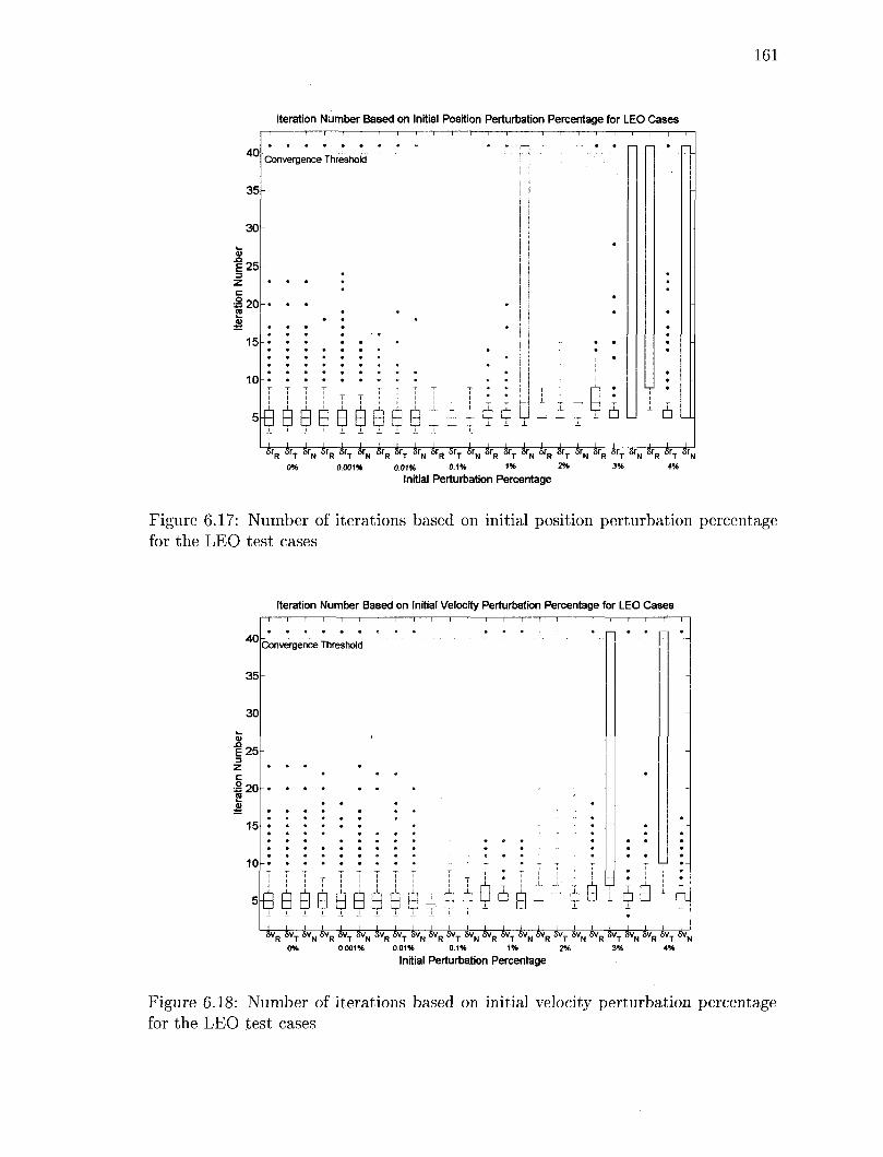
161

Iteration Number Based on Initial Position Perturbation Percentage for LEO Cases

40

35

30

1 251

Convergence Threshold

15h

10

4 B B B B B B B B B : : 51 a u n

8rR 8rT 8rN 8rR SrT irN 8rR 8rT 8rN SrR f>rT 8rN 8rR 8rT 8rN 8rR 8rT f>rN 8rR 8rT i7N 8rR 8rT sVJ


Figure 6.17: Number of iterations based on initial position perturbation percentage for the LEO test cases

Iteration Number Based on Initial Velocity Perturbation Percentage for LEO Cases - i 1 1 1 1 1 1 r~

40

35

30

1251

I 20

Convergence Threshold

15

10

5 H B B B B B 3 B S i r j . ± ± 0 i i - - - i B T 6 B i

B Q\

SvR SvT SvN 8VR 8vT 8vN SvR SvT 8vN 8vR 8vT 8VN SvR 8vy SvN SvR SvT 8vN 8VR SvT SvN 5vR SVT 8VN

0% 0 0 0 1 % 0.01% 0.1% 1 % 2% 3% 4%


Figure 6.18: Number of iterations based on initial velocity perturbation percentage for the LEO test cases

162

6.4 Conclusions

The following section details the limitations of the Cowell-STM method for low Earth

orbit transfer applications as well as summarizes the findings from the test cases.

6.4.1 Method Limitations

One major limitation on the predictor-corrector method for low Earth orbits is its

inability to handle perfect 180° transfers. For orbits with Au = 180°, a transfer solu

tion is difficult to determine because multiple answers produce the same final position

vector. Furthermore, the plane of the transfer orbit is not uniquely determined and

thus an infinite number of paths are feasible. Figure 6.19 shows an example of an

attempt to transfer 180° between two circular orbits at an inclination of 30°. The

predictor-corrector attempts multiple trajectory paths over a range of planes before

hitting the maximum number of iterations. The initial trajectories are those plot

ted in blue which each successive attempt plotted in a warmer color with the last

iteration in red. The trend of the 40 trajectories illustrates the corrector attempting

trajectories further out of plane from the initial guess each try. By the last failing

correction, the trajectory is over 90° out of plane compared to the initial Lambert

2-body guess. For two unique orbits the predictor-corrector can handle 180° trans

fers. These transfers are for equatorial (i = 0°) or polar (i = 90°) orbits. Orbits

with these characteristics have motion in only two planes: an equatorial orbit has no

motion in the z-plane and a polar orbit has no motion in the x-plane. As the Cowell

method makes corrections to the initial velocity it does so keeping each propagation

within the correct two planes. Hence, unlike the case illustrated in Figure 6.19 where

the predictor-correcter guesses trajectories outside of the initial orbit plane, guesses

made for equatorial or polar orbits stay in plane. Reducing the extra complexity in

motion, the tool is able to converge at a much quicker rate. This is not the case for

163

Convergence Failure Between Two Circular Orbits with a

Transfer Angle of 180° and an Inclination of 30°

Figure 6.19: Convergence failure for a LEO trajectory between two circular orbits with a transfer angle of 180° and an inclination of 30°

any inclined orbits in which every test with a 180° transfer angle fails to converge.

Further analysis on this issue shows that cases with a transfer angle of 180° produce

results similar to Rosenbrock's banana function. Rosenbrock's function is a classic op

timization problem whose global optimum is inside a long, narrow, parabolic-shaped

flat valley. To find the valley is not difficult, however to converge to the global op

timum in the valley is far more complex. As a result, Rosenbrock's function is often

used to assess the performance of optimization algorithms [11]. Figure 6.20 depicts

the evaluation of Rosenbrock's banana function plotted over two variables (x,y).

Selecting an initial velocity based on converged solutions of orbits with transfer

angles of 179° — 181°, a 180° transfer with an inclination of 45° is propagated out

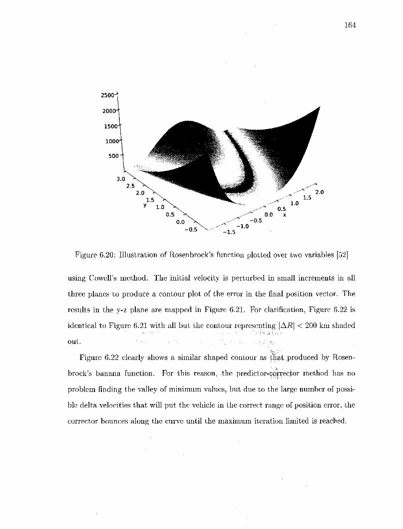
164

Figure 6.20: Illustration of Rosenbrock's function plotted over two variables [52]

using Cowell's method. The initial velocity is perturbed in small increments in all

three planes to produce a contour plot of the error in the final position vector. The

results in the y-z plane are mapped in Figure 6.21. For clarification, Figure 6.22 is

identical to Figure 6.21 with all but the contour representing |Ai?| < 200 km shaded

O U t . - i. . • . . . ' ! ;

Figure 6.22 clearly shows a similar shaped contour as that produced by Rosen-

brock's banana function. For this reason, the predictor-cprrector method has no

problem finding the valley of minimum values, but due to the large number of possi

ble delta velocities that will put the vehicle in the correct range of position error, the

corrector bounces along the curve until the maximum iteration limited is reached.

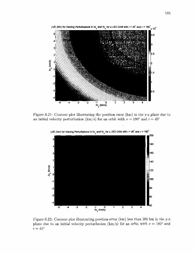
165

|AR| (km) for Varying Perturbations in 5v and 8v for a LEO Orbit with i = 45 and v = 180

Sv (km/s)

x10

3.5

Figure 6.21: Contour plot illustrating the position error (km) in the y-z plane due to an initial velocity perturbation (km/s) for an orbit with u = 180° and i = 45°

|AR| (km) for Varying Perturbations in 8v and 8v for a LEO Orbit with i = 45 and v = 180

-1 0 Sv (km/s)

Figure 6.22: Contour plot illustrating position error (km) less than 200 km in the y-z plane due to an initial velocity perturbation (km/s) for an orbit with v = 180° and i = 45°

166

Further, by re-examining Figure 6.21 it is easy to see why cases have issues con

verging in these situations: a guess of even 0.5 km/s in the wrong direction and

the |Ai?| jumps to over 1,000 km. For comparison, similar plots are produced for a

transfer angle of 160° and an inclination of 45° which easily converged on a solution.

Figure 6.23 is the contour plot and Figure 6.24 is the same plot with only the contours

representing \AR\ < 200 km highlighted. For the 160° transfer angle the range of

possible velocities that results in low position errors is very small. Since the shooting

method has so few velocities to attempt, it not only can find a solution, but in cases

such as these in which the possible velocities are very limited, convergence occurs

much more quickly as well. For the contour plots in the remaining planes (x-y and

x-z) please refer to Appendix D. These plots highlight that majority of the velocity

complexity occurs in the y-z plane.

Sv (km/s)

Figure 6.23: Contour plot illustrating the position error (km) in the y-z plane due to an initial velocity perturbation (km/s) for an orbit with v = 160° and i = 45°

167

| iR| (km) for Varying Perturbations of 8v and 8vz for a LEO Orbit with i = 45' and v = 160'

Sv (km/s)

Figure 6.24: Contour plot illustrating position error (km) less than 200 km in the y-z plane due to an initial velocity perturbation (km/s) for an orbit with v = 160° and i = 45°

6.4.2 Summary of Test Results

Utilizing the Cowell-STM algorithm to correct the transfer velocities produced by

Lambert 2-body dynamics points out a number of sensitivities to the method. Larger

iteration numbers are indicative of sensitivities to the predictor-corrector method,

whereas larger changes in velocity highlight weaknesses in the Lambert routine to

calculate accurate transfer velocities.

The altitude of the final orbit plays little role in the number of iterations required

to reach a converged solution. Analyzing the effects of eccentricity, orbits with eccen

tricities of 0.9 require the largest number of iterations. This is due to the longer time

of flight required to transfer to highly elliptical orbits, 200,000 seconds as compared to

4,000 seconds for circular orbits. Since the STM is numerically integrated, the longer

the matrix is propagated, the more inaccurate it becomes. As the matrix deviates

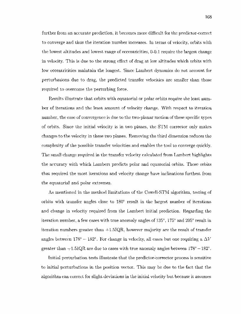
168

further from an accurate prediction, it becomes more difficult for the predictor-correct

to converge and thus the iteration number increases. In terms of velocity, orbits with

the lowest altitudes and lowest range of eccentricities, 0-0.1 require the largest change

in velocity. This is due to the strong effect of drag at low altitudes which orbits with

low eccentricities maintain the longest. Since Lambert dynamics do not account for

perturbations due to drag, the predicted transfer velocities are smaller than those

required to overcome the perturbing force.

Results illustrate that orbits with equatorial or polar orbits require the least num

ber of iterations and the least amount of velocity change. With respect to iteration

number, the ease of convergence is due to the two-planar motion of these specific types

of orbits. Since the initial velocity is in two planes, the STM corrector only makes

changes to the velocity in these two planes. Removing the third dimension reduces the

complexity of the possible transfer velocities and enables the tool to converge quickly.

The small change required in the transfer velocity calculated from Lambert highlights

the accuracy with which Lambert predicts polar and equatorial orbits. Those orbits

that required the most iterations and velocity change have inclinations furthest from

the equatorial and polar extremes.

As mentioned in the method limitations of the Cowell-STM algorithm, testing of

orbits with transfer angles close to 180° result in the largest number of iterations

and change in velocity required from the Lambert initial prediction. Regarding the

iteration number, a few cases with true anomaly angles of 135°, 175° and 205° result in

iteration numbers greater than +1.5IQR, however majority are the result of transfer

angles between 178° — 182°. For change in velocity, all cases but one requiring a AV

greater than +1.5IQR are due to cases with true anomaly angles between 178° —182°.

Initial perturbation tests illustrate that the predictor-corrector process is sensitive

to initial perturbations in the position vector. This may be due to the fact that the

algorithm can correct for slight deviations in the initial velocity but because it assumes

169

the initial position is constant, no corrections can be made to the position vector.

Since the transfer velocity predicted by Lambert is based on the same assumption

that r0 is constant, the perturbations to this vector can become only so large before the

velocity corrections become too non-linear for the state transition matrix to correct.

Chapter 7

Closure

The following chapter summarizes the results of applying the Cowell-STM algorithm

to translunar and low Earth orbit applications. It concludes with a look at potential

future work to improve the method.

In order to more accurately predict the transfer velocities required for translunar

and low Earth orbit transfers and produce realistic reference trajectories, a predictor-

corrector method was developed to qualify the velocities determined by low fidelity

models. The Cowell-STM method has real world application in navigation perfor

mance, delta velocity trade studies, and mission planning. The algorithm is signif

icant in that the more accurate the transfer velocities are known prior to mission

fly out, the less navigation correction is required resulting in a more cost-effective

mission.

The method utilizes Cowell's method with high order perturbation models as the

predicting propagator and a state transition matrix with lower order perturbation

models as the corrector. The perturbation accelerations implemented in Cowell's

method include solar and lunar correction terms, higher order Earth and lunar grav

ity up to degree 9, atmospheric drag, and solar radiation pressure. The state tran

sition matrix used for the translunar cases implemented 4-body motion and the J2

170

171

gravity coefficient. The STM used in the low Earth orbit cases included the same

perturbations as those for the translunar case, however drag was added as well. The

selection of these particular low order models was based on a study between com

putation time and accuracy of the matrix. By reducing the matrix to include only

those models listed, the predictor-corrector could calculate converged solutions in a

reasonable amount of computational time. If higher order terms are needed, the same

methodology presented in Chapter 4 may be followed to implement these terms.

For translunar cases, the Cowell predictor-corrector refined transfer velocities pro

duced by the multi-conic propagator EXLX. EXLX approximates translunar trajec

tories using the three-body pseudostate theory to compute overlapped conic transfer

trajectories between the Earth and Moon. All parameters of the test cases were

held constant except the Earth and lunar inclinations and ascending nodes. Only

those cases that met the AV maximum constraint reasonable for a Crew Exploration

Vehicle type mission were tested.

Of the 110 cases tested all converged using the predictor-corrector tool. Those

cases that required a larger number of iterations were found to switch between pro-

grade and retrograde orbits. This change in direction also required a larger change

in transfer velocity from the initial value produced by EXLX. The reversal of lunar

orbit direction was a result of higher order gravity perturbations near the Moon.

Due to the fact that EXLX does not model high order lunar gravity, its predicted

transfer trajectories took paths that were not feasible with the Cowell propagator.

In these cases, only by switching the direction of the final orbit motion could the

predictor-corrector converge on a solution.

Testing on initial orbit perturbations illustrated that all cases failed to converge

if a perturbation of only 4% was applied to the initial states. This illustrates how

sensitive the process is to the relative accuracy of the initial guess.

For low Earth orbit cases, Lambert's method was used to produce initial trans-

172

fer velocity guesses for the Cowell-STM method. The altitude, eccentricity, incli

nation, and true anomaly of the orbits varied for each test case. Testing was done

to illustrate the effect of different orbit transfers on iteration number and change in

predicted transfer velocity. Higher iteration numbers were indicative of sensitivities

towards particular orbital parameters in the predictor-corrector process, whereas high

velocity changes pointed to a weakness in the Lambert method for calculating accu

rate velocities. Concerning altitude, results highlighted little correlation between the

initial altitude of the orbit and iteration number or change in velocity.

Results illustrated that orbits with the highest eccentricity of 0.9 required the

most iterations, but orbits with low eccentricities of 0-0.1 required the most change

in velocity. The first observation is a result of highly elliptical orbits requiring longer

transfer times. The longer the STM is propagated for, the more inaccurate it be

comes due to numerical roundoff making it more difficult for the predictor-corrector

to converge on a solution. The second observation is due to the large effect of drag

on vehicles orbiting at low altitudes. Lambert's method assumes no drag in its cal

culations thus for situations in which drag is present a much larger transfer velocity

is required to reach the desired final position in the given transfer time.

Concerning inclination, testing showed that polar and equatorial orbits converged

the most quickly. Since these orbits are defined in two planes, the Lambert shooting

method makes velocity corrections in only two of the possible three directions. Due

to this decrease in complexity, equatorial and polar orbits are more likely to converge

in the fewest number of iterations.

With respect to true anomaly, preliminary testing showed the predictor-corrector

algorithm could not handle transfer angles of exactly 180° for inclined orbits due to

the difficulty of the solution space. For situations in which the transfer angle was 180°

the allowable deviation in initial transfer velocity to produce a viable final position

error becomes much tighter. Consequently, the algorithm makes multiple attempts

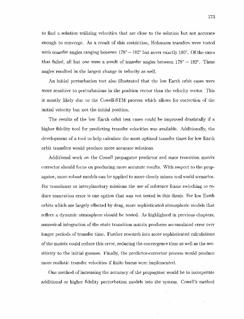
173

to find a solution utilizing velocities that are close to the solution but not accurate

enough to converge. As a result of this restriction, Hohmann transfers were tested

with transfer angles ranging between 178° — 182° but never exactly 180°. Of the cases

that failed, all but one were a result of transfer angles between 178° — 182°. These

angles resulted in the largest change in velocity as well.

An initial perturbation test also illustrated that the low Earth orbit cases were

more sensitive to perturbations in the position vector than the velocity vector. This

is mostly likely due to the Cowell-STM process which allows for correction of the

initial velocity but not the initial position.

The results of the low Earth orbit test cases could be improved drastically if a

higher fidelity tool for predicting transfer velocities was available. Additionally, the

development of a tool to help calculate the most optimal transfer times for low Earth

orbit transfers would produce more accurate solutions.

Additional work on the Cowell propagator predictor and state transition matrix

corrector should focus on producing more accurate results. With respect to the prop

agator, more robust models can be applied to more closely mirror real world scenarios.

For translunar or interplanetary missions the use of reference frame switching to re

duce truncation error is one option that was not tested in this thesis. For low Earth

orbits which are largely effected by drag, more sophisticated atmospheric models that

reflect a dynamic atmosphere should be tested. As highlighted in previous chapters,

numerical integration of the state transition matrix produces accumulated error over

longer periods of transfer time. Further research into more sophisticated calculations

of the matrix could reduce this error, reducing the convergence time as well as the sen

sitivity to the initial guesses. Finally, the predictor-corrector process would produce

more realistic transfer velocities if finite burns were implemented.

One method of increasing the accuracy of the propagator would be to incorporate

additional or higher fidelity perturbation models into the system. Cowell's method

174

relies on the calculation of a vehicle's state around a primary body. However, studies

show that in transplanetary missions there is a point at which the Earth is no longer

the primary body and the reference frame should switch to reduce round off error [50].

Reference frame switching, which is also used by the pseudostate method applied in

EXLX, has the benefit of utilizing smaller state vectors to reduce round-off errors

in calculations. This switch is dictated by the location of the vehicle with respect

to the sphere of influence of each respective planet. The frame switch issue is best

understood when viewing the spheres of influence of different planets as nested spheres

all within the greater sphere of the sun. Figure 7.1 illustrates this concept.

Figure 7.1: Spheres of influence for the Sun, Mercury, Venus, Earth, Moon, and Mars.

If frame switching logic were implemented, additional bodies should be added to

the model to enable interplanetary missions. Information on the planet structure as

well as any known gravity coefficients should be included as well.

With respect to low Earth orbits, higher fidelity atmospheric models should be

implemented. The simplistic model applied in this research assumed many atmo

spheric parameters remained constant and thus does not accurately reflect real world

effects. Unlike the static model used in this research, time varying models can take

into consideration diurnal variations, the solar rotation cycle, seasonal variations,

magnetic storm variations, and the rotating atmosphere to name a few. One of the

most complete time-varying models is the Jaccia-Roberts atmosphere which contains

175

analytical expressions for calculating exospheric temperature as a function of posi

tion, time, solar activity, and geomagnetic activity. Density is determined from the

exospheric temperature using temperature profiles or from the diffusion equation.

However, as the most high fidelity model, the Jaccia-Roberts atmosphere also re

quires the most computational time [49]. If the computational cost of time-varying

models it too great, high order static models such as the Harris-Priester model should

be considered.

One of the major factors contributing to the iteration number in the predictor-

corrector process is the level of accuracy of the state transition matrix. Even with

no perturbations, the matrix produces errors that only increase as the time of flight

increases. A more accurate state transition matrix would reduce the number of itera

tions required for convergence. One such method is the sensitivity matrix algorithm

developed by Bryson and Ho and discussed by Der and Danchick [26] [18, 19] .

Finally, note that all burns calculated and implemented in this work were assumed

to be purely impulsive burns. Realistically, burns occur over a finite period of time and

modeling them in this way would provide more accurate initial burn velocities. For

simplicity, the burn acceleration could be modeled assuming a constant acceleration,

Umax- The total burn time could then be calculated using thurn = - ^ - , where AV Umax

is the burn velocity provided by EXLX or Lambert. The start time for the burn

must occur earlier now due to its finite nature. Assuming t* represents the burn

start time for the impulsive case, one definition of the start time for the finite burn

could be tburno = t* — ^tbum. Using this as the start time, the states are propagated

forward using the Cowell method to t*, however, because of the perturbations applied

in the model the final states at t* will not match those used by EXLX or Lambert to

calculate the transfer velocity. Thus a shooting method is required to determine the

initial velocity that when propagated over a finite period of time results in final states

at t* that are within some tolerance of the initial states used by the impulsive burn.

176

From here an additional level of targeting is used to determine the transfer velocity

from t* to tf. This targeting is the premise behind the research in this thesis. Each

time the second level updates its initial conditions at t* the conditions at tburn0 must

be updated as well. Thus two-level targeting is required to implement finite burns

into the predictor-corrector method.

As with any addition of a more complex algorithm, adding finite burns into the

process will increase the require computational time. A trade study between accuracy

and computation time must be made prior to implementing any of the future work

just described.

Appendix A

Feasible Translunar Trajectories

The following contour plots (Figure A.1-A.8) represent the feasible lunar orbital el

ement ranges for initial Earth orbits with varying inclinations and ascending nodes.

The information was collected from a number of multi-conic runs produced by EXLX

scans. The plots highlight a tendency for certain values of the Earth and lunar param

eters to produce infeasible translunar transfers as determined by the maximum lunar

orbit insertion velocity constraint placed on EXLX. The contour lines are indicative

of the Moon's geometry for the transfer date selected. Note for cases in which the

Earth orbit is equatorial, % = 0°, the horizontal asymptotic bands around iQ = 0°

and i 0 = 180° and the vertical bands around fi0 = 90° and fiQ = 270 indicate the

largest regions of feasibility. For an initial equatorial Earth orbit the vehicle will al

ways be able to enter into an equatorial lunar orbit. From the orientation of the Moon

compared to the Earth, the vehicle will expend the least amount of velocity entering

a lunar equatorial orbit at the nodes, either f2Q = 90° or QQ = 270° depending on the

direction of motion. The contour lines place boundaries on how the orbital elements

were selected for testing of the translunar cases.

177

Feasible Lunar Parameters for Earth Orbit of Varying Inclinations and Q = 0

350

300

1250

£200

t u

Sel

enog

8

50

r>

i i

"'"——-—. i - - 1 - i

'S~~ - _ ~ ~ " ^ ^ N i

NN / \ /^ - \ :.

\

::.jrj

;

i^ j / ^ 7 i ; ~~^\

/ - • • •

1 ;

\ ;

— — - * — • i i i i i • •

1

© j = 0° i = 45

- -

: -

- -

-=•:_ J S ' - ™ - | —

50 100 150 200 250 300 Selenographic Longitude of Ascending Node (deg)

350

Figure A.l: Feasible lunar orbit parameters for an initial Earth orbit with varying inclinations and f2ffi = 0°



350

Figure A.2: Feasible lunar orbit parameters for an initial Earth orbit with varying inclinations and Jlffi = 45°


"b 50 100 150 200 250 300 350 Selenographic Longitude of Ascending Node (deg)

Figure A.3: Feasible lunar orbit parameters for an initial Earth orbit with varying inclinations and fie = 90°


o' - ~ r / i — i 1 rcr—^ 1 r-0 50 100 150 200 250 300 350

Selenographic Longitude of Ascending Node (deg)

Figure A.4: Feasible lunar orbit parameters for an initial Earth orbit with varying inclinations and O© = 135°

' '•: V' ' ... / '.',' i".r(i..ir- . .

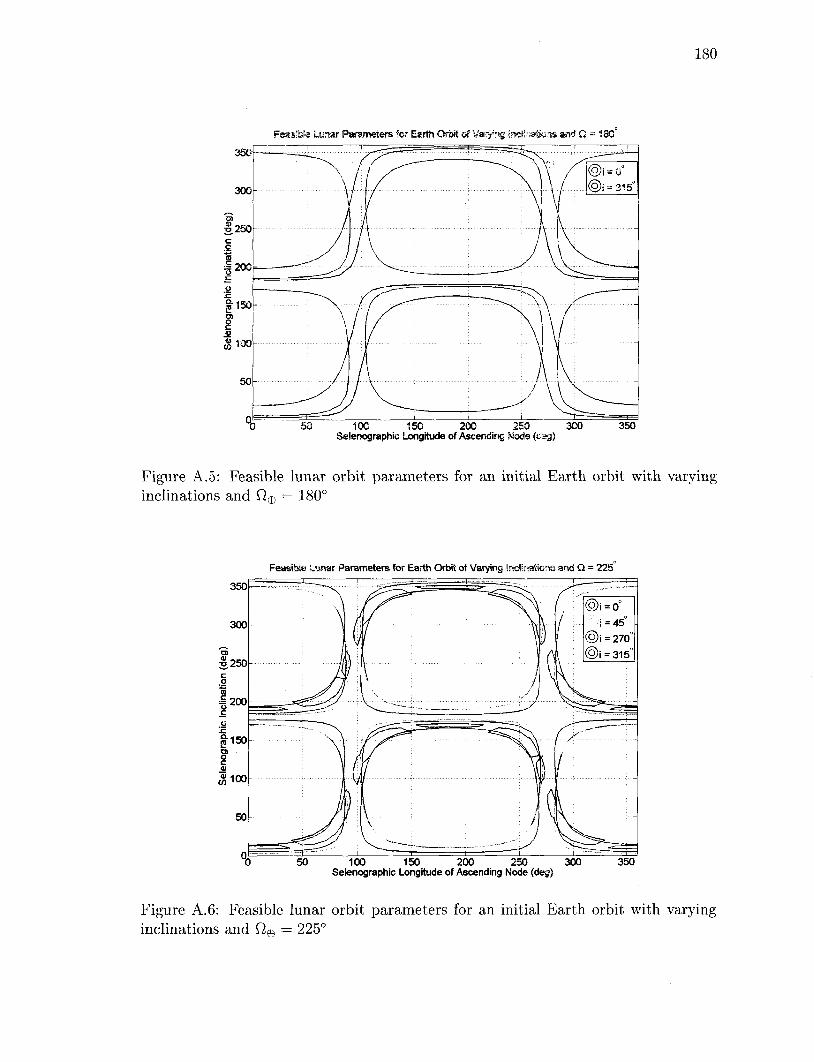
Feasib'e Lunar Parameters for Earth Orbit of Varying IndinsSiorss and Q = 180

"b 50 100 150 200 250 300 350 Selsnographic Longitude of Ascending Mode (dag)

Figure A.5: Feasible lunar orbit parameters for an initial Earth orbit with varying inclinations and fi® = 180°


Figure A.6: Feasible lunar orbit parameters for an initial Earth orbit with varying inclinations and fi® = 225°

181


100 1,50 200 250 Selenographic Longitude of Ascending Node

Figure A.7: Feasible lunar orbit parameters for an initial Earth orbit with varying inclinations and Qffi = 270°

Feasible Lunar Parameters for Earth Orbit of Varying, Inclinatiipns. and Q = 315


Figure A.8: Feasible lunar orbit parameters for an initial Earth orbit with varying inclinations and fiffi = 315°

Appendix B

Monte Carlo Sample Size

Due to the time consuming manual process required to run multiple EXLX trajec

tories a reasonable minimum number of test cases was desired for Monte Carlo runs

[36] [35] [46]. Preliminary testing illustrated all initial test cases converged (i.e. apply

ing the shooting method with the Cowell propagator resulted in a converged solution

under 40 iterations each time). With a probability of success close to 1 the following

process was utilized to determine the minimal sample size.

A one-sided confidence interval with the probability of success, p is defined as:

100(1 -a)% (B.l)

For a Monte Carlo sample size, n, the probability of obtaining n successes is pn.

Solving for pL from the equation p\ = a results in the lower bound on the probability

of success with 100(1 — a)% confidence. The value of n is thus:

n = (B.2) log PL

For a probability of success of 0.95 with a 95% confidence level, the minimum re

quired number of samples is 59. As aforementioned, this number only holds up if the

182

183

probability of success is very close to 1 in reality. The final number of translunar test

cases selected for testing was 110. As discussed in Chapter 5, all cases converged.

Because the probability of success is so high the confidence level for the tool remains

above 95% despite the small number of runs performed.

Appendix C

List of Test Cases

The following table details the parameters selected for each translunar test case:

Case #

1 2 3 4 5 6 7 8 9 10 11 12 13 14 15 16 17 18 19 20 21

Earth i^

30 40 40 90 5 10 2 55 78 45 62 0 0 100 33 64 52 69 14 10 24

Earth n°e

0 50 50 20 130 20 1 1 50 75 32 0 0 32 17 308 28 67 151 18 177

Moon i°Q

5 15 25 25 45 10 0 50 69 75 38 0 30 90 127 20 109 125 132 6 149

Moon Q Q

330 45 100 60 120 120 240 320 290 110 50 85 105 100 108 59 273 94 96 328 89

Iterations

8 27 10 22 13 14 12 10 11 10 17 17 20 10 9 14 11 11 11 22 15

184

Case # 22 23 24 25 26 27 28 29 30 31 32 33 34 35 36 37 38 39 40 41 42 43 44 45 46 47 48 49 50 51 52 53 54 55 56 57 58 59 60

Earth i°&

85 3 61 106 99 52 69 103 14 10 96 24 103 85 3 61 30 30 48 16 42 64 73 44 23 44 10 49 77 76 55 33 24 31 6 35 83 29 68

Earth %

325 133 41 33 48 25 99 27 154 112 64 14 44 23 34 44 76 89 61 71 44 88 81 92 92 144 241 125 281 217 330 117 283 13 64 123 70 88 276

Moon i°Q

170 5 50 135 25 14 141 35 178 140 128 26 132 112 178 144 116 44 158 55 125 289 315 176 199 216 148 107 5 20 97 115 7 28 96 180 116 10 77

Moon [}g

189 198 93 109 69 22 97 72 16 88 105 92 108 105 103 103 94 89 123 100 265 280 257 353 257 270 278 279 150 113 270 279 233 291 97 189 99 60 102

Iterations

11 20 11 11 19 22 7 21 10 8 12 19 16 7 8 8 10 30 7 17 10 11 27 8 9 11 8 9 15 18 16 8 26 17 25 14 8 18 11

Case #

61 62 63 64 65 66 67 68 69 70 71 72 73 74 75 76 77 78 79 80 81 82 83 84 85 86 87 88 89 90 91 92 93 94 95 96 97 98 99 100

Earth i^

35 87 22 46 53 48 62 20 78 48 27 64 35 76 81 1 1 8 24 3 31 27 31 78 31 310 355 340 355 300 345 45 333 6 351 311 10 310 315 319

Earth %

68 33 208 234 245 341 43 163 50 309 139 251 227 342 31 212 316 169 158 269 310 176 83 31 25 40 266 280 325 299 75 312 277 200 182 200 140 125 135 85

Moon i°& Moon Q°Q

7 1 132

38 21 94 180 173 121 3 20 6 129 178 169 17 117 23 113 22 115 131 106 28 12 90 13 300 335 250 210 260 280 182 356 352 347 344 357 359 360 251

287 278 271 34 191 262 188 75 320 89 4 274 35 107 261 274 117 91 271 275 270 72 281 301 100 108 103 95 96 91 70 200 3 53 148 252 303 350 273

Iterations

17 14 10 14 8 10 8 21 12 21 11 11 7 11 8 14 9 25 14 8 13 16 16 23 8 12 26 9 13 11 12 10 14 16 23 22 24 31 34 11

Case #

101 102 103 104 105 106 107 108 109 110

Earth i^

320 330 303 320 321 312 314 310 325 318

Earth fi|

50 170 230 285 275 60 226 35 100 220

Moon i°Q

175 167 185 183 243 204 274 223 319 340

Moon tt°&

149 225 300 325 270 273 268 101 95 277

Iterations

10 9 12 10 11 11 11 9 16 18

Table C.l: List of parameters for translunar test cases

Appendix D

LEO Contour Maps

The following contour plots depict the error in position due to velocity perturbations

in the x-z and x-y planes for transfer angles of 180° and 160° with orbit inclinations

of 45°. Each two plots is a set with the first plot depicting the entire range of position

errors and the second plot focused on just the contours that produce position errors

less than 200 km. Compared to the plots in Section 6.4.1, it is clear that most of the

error complexity comes from perturbations in the y-z plane. Velocity perturbations

in the x-z and x-y planes highlight very specific regions of acceptable velocities thus

a converged solution is much easier to achieve.

188

189

I (km) for Varying Perturbations in Sv and 5v for a LEO Orbit with I = 45 and v = 180 . T x10

fejl|ifc ^FW^SMfp^^M^PJI

' • • " • » & • < & # !

• . - . • , - • * • ! ^ W : » • * -* . . " \ « i «••-»

V- • .•"•!!• J: V..J"J! - • . • . . • " • • V l " > ^ 1

, ~ . • • " • " \ ' « * . f " i - ' - i

' .- .• .-• . '•^'SV-.-T

^2.5

I 1 5

10.5

1 0 1 8v (km/s)

Figure D.l: Contour plot illustrating the position error (km) in the x-z plane due to an initial velocity perturbation (km/s) for an orbit with v = 180° and i = 45°

|AR| (km) for Varying Perturbations in 5v and 8v for a LEO Orbit with i = 45 and v :

51

180

-1 0 1 8v (km/s)

Figure D.2: Contour plot illustrating position error (km) less than 200 km in the x-z plane due to an initial velocity perturbation (km/s) for an orbit with u = 180° and i = 45°

190

|AR| (km) for Varying Perturbations in Sv and Sv for a LEO Orbit with i - 45 and v = 180 x10

3.5

2.5

1.5

3.5

0 Sv (km/s)

Figure D.3: Contour plot illustrating the position error (km) in the x-y plane due to an initial velocity perturbation (km/s) for an orbit with u = 180° and i = 45°

|AR| (km) for Varying Perturbations in 5v and Sv for a LEO Orbit with i = 45 and v = 180

JC

^

-1 0 1 Sv (km/s)

Figure D.4: Contour plot illustrating position error (km) less than 200 km in the x-y plane due to an initial velocity perturbation (km/s) for an orbit with v = 180° and i = 45° ...

191

|AR| (km) for Varying Perturbations in 8v and Sv for LEO Orbit with i = 45 and v = 160 . c x z x10

-1 0 1 Sv (km/s)

Figure D.5: Contour plot illustrating the position error (km) in the x-z plane due to an initial velocity perturbation (km/s) for an orbit with v = 160° and i = 45°

|AR| (km) for Varying Perturbations in Sv and Sv for LEO Orbit with i = 45 and v = 160

-1 0 1 Sv (km/s)

Figure D.6: Contour plot illustrating position error (km) less than 200 km in the x-z plane due to an initial velocity perturbation (km/s) for an orbit with v = 160° and i = 45°

192

|AR| (km) for Varying Perturbations in 8v and Sv for a LEO Orbit with I = 45 and v :

x y

8v (km/s)

Figure D.7: Contour plot illustrating the position error (km) in the x-y plane due to an initial velocity perturbation (km/s) for an orbit with v = 160° and i = 45°

|AR| (km) for Perturbations in Sv and 8v for a LEO Orbit with i = 45 and v = 160

0 Sv (km/s)

Figure D.8: Contour plot illustrating position error (km) less than 200 km in the x-y plane due to an initial velocity perturbation (km/s) for an orbit with v = 160° and i = 45°

Bibliography

[1] MATLAB 7.6.0 (R2008a) Help Manual.

[2] Oceanographers catch first wave of gravity mission's success. Jet Propulsion

Laboratory: www.jpl.nasa.gov/news/news.cfm?release=2003-103, July 2003.

[3] Naif planetary data system navigation node. NASA:

naif.jpl.nasa.gov/naif/index.html, Nov 2009.

[4] R. L. Alford and J. J. F. Liu. Application of encke's method for low-earth orbit

determination. American Astronomical Society, (No. -85-354).

[5] F. Amato. Robust Control of Linear Systems Subject to Time-Varying Parame

ters. Springer-Verlag, Berlin, Germany, 2006.

[6] R. R. Bate, D. D. Mueller, and J. E. White. Fundamentals of Astrodynamics.

Dover Publications, Inc., 1971.

[7] R. H. Battin. An Introduction to the Mathematics and Methods of Astrodynamics.

American Institute of Aeronautics and Astronautics, Reston, VA, revised edition,

1999. .. I,.i.,v,v,rvil„ir,!.., , . .••.-...'..v.,-itn;-..-•. -

[8] J. T. Betts. Practical Method for Optimal Control Using Nonlinear Programming.

Society for Industrial and Applied Mathematics, Philadelphia, PA, 2001.

[9] D. Brouwer and G.M. Clemence. Methods of Celestial Mechanics. Academic

Press Inc., 1961.

193

http://www.jpl.nasa.gov/news/news.cfm?release=2003-103

http://naif.jpl.nasa.gov/naif/index.html

194

[10] C. D. Brown. Spacecraft Mission Design. American Institute of Aeronautics and

Astronautics, Reston, VA, 2nd edition, 1998.

[11] G. Buttazzo and A. Frediani, editors. Variational Analysis and Aerospace Engi

neering. Springer Science+Business Media, New York, NY, 2000.

[12] D. V. Byrnes. Application of the pseudostate theory to the three-body lambert

problem. The Journal of the Astronautical Sciences, Vol. 37(No. 3):221-232,

July-September 1989.

[13] D. V. Byrnes and H. L. Hooper. Multi-conic: A fast and accurate methode

of computing space flight trajectories. American Institute of Aeronautics and

Astronautics, (No. 70-1062), August 1970.

[14] V. A. Chobotov, editor. Orbital Mechanics. American Institute of Aeronautics

and Astronautics, 2002.

[15] G. L. Condon. Lunar orbit insertion targeting and associated outbound mission

design for lunar sortie missions. Hilton Head, South Carolina, 20-23 August

2007. AIAA Guidance, Navigation and Control Conference and Exhibit.

[16] L. D'Amario and T.N. Edelbaum. Minimum impulse three-body trajectories.

American Institute of Aeronautics and Astronautics, (Paper 73-145), Feb 1973.

[17] J. M. A. Danby. Fundamentals of Celestial Mechanics. Willmann-Bell, Inc.,

Richmond, VA, 2nd edition, 1988.

[18] G. J. Der. An elegant state transition matrix. American Institute of Aeronautics

and Astronautics, (A9634790):776-791, July 1996.

[19] G. J. Der and R. Danchick. Analytical and numerical error covariance matrix

propagation (for spacecraft in earth orbital environments). American Institute

of Aeronautics and Astronautics, (A9634798):854-878, July 1996.

195

[20] C. D'Souza. The mathematical foundations and framework for the orion high-

accuracy encke-nystrom trajectory integrator. Unpublished manuscript, June

2008.

[21] V.A. Egorov. Certain problems of moon flight dynamics. Russian Literature of

Satellites, Part I, International Physical Index, Inc., 1958.

[22] P. R. Escobal. Methods of Orbit Determination. R. E. Krieger Publishing Com

pany, 1965.

[23] G. S. Gideon. A practical note on the use of lambert's equation. American

Institute of Aeronautics and Astronautics, Vol. 3(No. 1), January 1965.

[24] Michael Douglas Griffin and James R. French. Space Vehicle Design. American

Institute of Aeronautics and Astronautics, 2nd edition, 2004.

[25] C. E. Velez J. O. Cappellari and A. J. Fuchs. Mathematical theory of the god-

dard trajectory determination system. Technical Report X-582-76-77, Goddard

Space Flight Center: National Aeronautics and Space Administration, Greenbelt,

Maryland, April 1976.

[26] A. E. Bryson Jr. and Y. Ho. Applied Optimal Control. Hemisphere Publishing

Corporation, Washington, D.C., 1975.

[27] W. H. Michael Jr. and W. T. Blackshear. Recent results on the mass, gravita

tional field and moments of inertia of the moon. Earth, Moon, and Planets, Vol.

3(No. 4):388-402, March 1972.

[28] A. Kharab and R. B. Guenther. An Introduction to Numerical Methods: A

MATLAB Approach. Chapman and Hall, 2nd edition, 2006.

196

[29] K. Kledron and T.H. Sweetser. A comparison of onestep and other multiconic

trajectory propagation methods. American Institute of Aeronautics and Astro

nautics, (Paper 88-4286), August 1988.

[30] D. V. Brynes L. A. D'Amario and R. H. Stanford. Interplanetary trajectory

optimization with application to galileo. American Institute of Aeronautics and

Astronautics, Vol. 5(Paper 82-4248), Sept-Oct 1982.

[31] E. R. Lancaster and R. C. Blanchard. A unified form of lambert's theorem. NASA

Technical Note TN D-5368, National Aeronautics and Space Administration,

1969.

[32] C. R. Mclnnes. Solar Sailing: Technology, Dynamics and Mission Applications.

Springer-Verlag, 1999.

[33] C. B. Moler. Numerical Computing with MATLAB. Society for Industrial and

Applied Mathematics, Philadelpha, PA, 2004.

[34] B. R. Rauschenbakh M. Y. Ovchinnikov and S. McKenna-Lawlor. Essential

Spaceflight Dynamics and Magnetospherics. Kluwer Academic Publishers, Dor

drecht, The Netherlands, 2003.

[35] D. A. Nelson P. D. Spanos, L. J. Mushung and D. A. Hamilton. Spectral rep

resentation of high-frequency space shuttle flight data. Journal of Aerospace

Engineering, 7(3), July 1994.

[36] D.A. Nelson P. D. Spanos, L. J. Mushung and D.A. Hamilton. Low frequency

spectral representation of space shuttle flight data. Journal of Aerospace Engi

neering, 3(2), April 1990.

[37] S. Pines. Uniform representation of the gravitational potential and its derivatives.

AIAA, Vol. 2(No.2), November 1973.

197

[38] Jr. R. Y. Roth R. J. Richard, V. C. Clarke and W. E. Kirhofer. Earth-moon

trajectories, 1965-70. Technical Report No. 32-503, National Aeronautics and

Space Administration, Jet Propulsion Laboratory. Pasadena, CA., November

1965.

[39] R.V. Ramanan and V. Adimurthy. Nonimpact lunar transfer trajectories using

the pseudostate technique. Journal of Guidance, Control, and Dynamics, Vol.

28(No. 2), March-April 2005.

[40] F. J. Regan and S. M. Anandakrishnan. Dynamics of Atmospheric Re-Entry.

American Institute of Aeronautics and Astronautics, 1993.

[41] C. Roithmayr. Contributions of spherical harmonics to magnetic and gravi

tational fields. Technical Report NASA/TM-2004-213007, National Aeronatics

and Space Administration, Langley Research Center, Hampton, Virginia, March

2004.

[42] A. E. Roy. Orbital Motion. Institute of Physics Publishing, 4th edition, 1978.

[43] H. Schaub and J. L. Junkins. Analytical Mechanics of Space Systems. American

Institute of Aeronautics and Astronautics, 2003.

[44] B. D. Tapley B. E. Schutz and G. H. Born. Statistical Orbit Determination.

Elsevier Academic Press, 2004.

[45] S. W. Shepperd. Universal keplerian state transition matrix. Celestial Mechanics,

Vol. 35, 1985.

[46] I.M. Sobol. A Primer for the Monte Carlo Method. CRC Press, Boca Raton,

FL, 1994.

198

[47] Jr. S.W. Wilson. A pseudostate theory for the approximation of three-body tra

jectories. Number AIAA Paper No. 70-1061. AAS/AIAA Astrodynamics Con

ference, Santa Barbara, California, 19-21 August 1970.

[48] The Analytic Sciences Corporation Technical Staff. Applied Optimal Control.

The MIT Press, 1974.

[49] D. A. Vallado. Fundamentals of Astrodynamics and Applications. Microcosm

Press and Springer, 3rd edition, 2007.

[50] M. P. Vautier and A. J. Sinclair. Effect of coordinate switching on translunar tra

jectory simulation accuracy. Honolulu, HI, 18-21 August 2008. AIAA Guidance,

Navigation and Control Conference and Exhibit.

[51] M. Wieczorek. Spherical harmonic models of planetary topography.

http://www.ipgp.fr/ wieczor/CrustalThicknessArchive/CrustalThickness.html.

Institut de Physique du Globe de Paris.

[52] Wikipedia. Rosenbrock function. http://en.wikipedia.org/wiki/Rosenbrockfunction.svg.

[53] D. Zwilinger. CRC Standard Mathematical Tables and Formulae. CRC Press,

1995.

http://www.ipgp.fr/

http://en.wikipedia.org/wiki/Rosenbrockfunction.svg

rice university on-orbit transfer trajectory methods … · · 2017-12-15on-orbit transfer...

Documents