Richardson Extrapolation Techniques for Pricing

American-style Options

Chuang-Chang Chang, San-Lin Chung1, and Richard C. Stapleton2

This Draft: May 21, 2001

1Department of Finance, The Management School, National Central University,

Chung-Li, Taiwan. Tel:886-3-4227424, Fax:886-3-42228912Department of Accounting and Finance, The Management School, Strathclyde

University, United Kingdom.

Abstract

In this paper we re-examine the Geske-Johnson formula (1984) and extend

the analysis by deriving a modified Geske-Johnson formula that can over-

come the possibility of non-uniform convergence encountered in the original

Geske-Johnson formula. Furthermore, we propose a numerical method, the

repeated Richardson extrapolation, which is able to estimate the interval of

true option values when the accelerated binomial option pricing models are

used to value American-style options. We also investigate the possibility

of combining the Binomial Black and Scholes method proposed by Broadie

and Detemple (1996) with the repeated Richardson extrapolation technique.

From the simulation results, our modified Breen accelerated binomial model

is as fast, but on average more accurate than, the Breen accelerated bino-

mial model. We lastly illustrate that the repeated Richardson extrapolation

approach can estimate the interval of true American option values extremely

well.

1 Introduction

In an important contribution, Geske and Johnson (1984) showed that it

was possible to value an American-style option by using a series of options

exercisable at one of a finite number of exercise points (known as Mid-

Atlantic or Bermuda options). They employed Richardson extrapolation

techniques to derive an efficient computational formula using the values of

Bermuda options. The Richardson extrapolation techniques were afterwards

used to enhance the computational efficiency and/or accuracy of American

option pricing in two directions in the literature. First, one can apply the

Richardson extrapolation in the number of time steps of binomial trees to

price options. For example, Broadie and Detemple (1996), Tian (1999),

and Heston and Zhou (2000) apply a two-point Richardson extrapolation to

the binomial option prices. Second, the Richardson extrapolation method

has been used to approximate the American option prices with a series of

options with an increasing number of exercise points. The existing literature

includes Breen (1991) and Bunch and Johnson (1992).

Two problems are recognized to exist with this methodology. First, as

pointed out by Omberg (1987), there may in the case of some options be

the problem of non-uniform convergence.1 In general, this arises when a1In the Geske-Johnson formula, they defined P (1), P (2) and P (3) as follows: (i) P(1)

is a European option, permitting exercise at time T , the maturity date of the option; (ii)

P (2) is the value of a Mid-Atlantic option, permitting exercise at time T/2 or T ; (iii) P(3)

is the value of a Mid-Atlantic option, permitting exercise at time T/3,2T/3, or T . Omberg

(1987) showed a plausible example of a non-uniform convergence with a deep-in-the-money

put option written on a low volatility, high dividend stock going ex-dividend once during

the term of the option at time T/2. In this case, there is a high probability that the option

will be exercised at time T/2 immediately after the stock goes ex-dividend. Thus, P(2)

1

Mid-Atlantic option with n exercise points has a value that is less than that

of an option with m exercise points, where m < n. A second problem with

the Geske-Johnson method is that it is difficult to determine the accuracy

of the approximation. How many options or how many exercise points have

to be considered in order to achieve a given level of accuracy?

In this paper we examine these two problems in the context of bino-

mial approximations of the underlying lognormal process generating asset

prices. Breen (1991) presented what he termed an accelerated binomial

model (henceforth refered to as the AB model) in which each of the op-

tions with 1, 2, 3,..,n exercise points is priced with a binomial model. This

technique is of interest, because it allows an evaluation of options where

n is relatively large, or where more than one variable affects the option’s

value. In these cases the use of a multivariate lognormal distribution may

become impractical. However, owing to employing the Geske-Johnson’s for-

mula, Breen’s accelerated binomial model may also encounter the problem of

non-uniform convergence. We solve these problems by introducing two tech-

niques from Richardson’s numerical approximation. In place of the arith-

metic time steps used by Geske-Johnson, we employ geometric time steps.

Secondly, we employ a technique known as repeated Richardson approximation.2

This helps to specify the accuracy of an approximation to the unknown true

option price, helping to determine the smallest value of n that can solely

be used in an option price approximation. We also investigate the pos-

sibility of combining the Binomial Black and Scholes (hereafter known as

will lead to be greater than P (3), and the problem of non-uniform convergence emerges.2We will discuss the repeated Richardson approximation techniques in details in section

4.

2

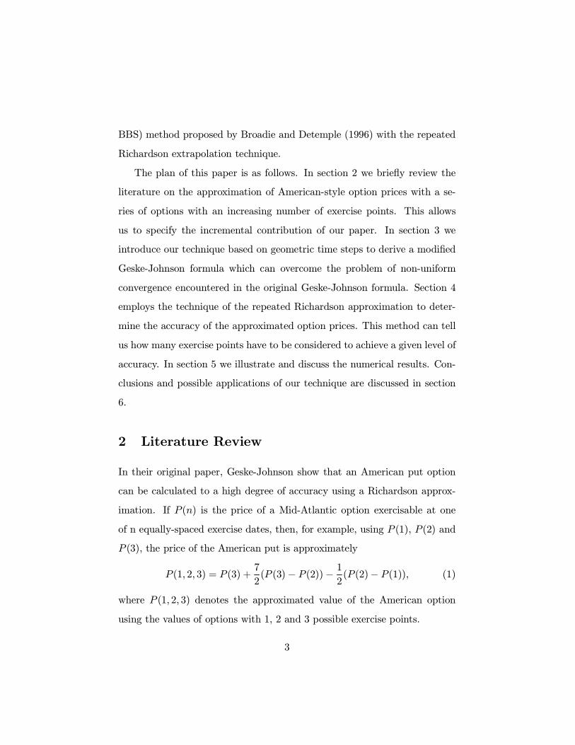
BBS) method proposed by Broadie and Detemple (1996) with the repeated

Richardson extrapolation technique.

The plan of this paper is as follows. In section 2 we briefly review the

literature on the approximation of American-style option prices with a se-

ries of options with an increasing number of exercise points. This allows

us to specify the incremental contribution of our paper. In section 3 we

introduce our technique based on geometric time steps to derive a modified

Geske-Johnson formula which can overcome the problem of non-uniform

convergence encountered in the original Geske-Johnson formula. Section 4

employs the technique of the repeated Richardson approximation to deter-

mine the accuracy of the approximated option prices. This method can tell

us how many exercise points have to be considered to achieve a given level of

accuracy. In section 5 we illustrate and discuss the numerical results. Con-

clusions and possible applications of our technique are discussed in section

6.

2 Literature Review

In their original paper, Geske-Johnson show that an American put option

can be calculated to a high degree of accuracy using a Richardson approx-

imation. If P (n) is the price of a Mid-Atlantic option exercisable at one

of n equally-spaced exercise dates, then, for example, using P (1), P (2) and

P (3), the price of the American put is approximately

P (1, 2, 3) = P (3) +7

2(P (3)− P (2))− 1

2(P (2)− P (1)), (1)

where P (1, 2, 3) denotes the approximated value of the American option

using the values of options with 1, 2 and 3 possible exercise points.

3

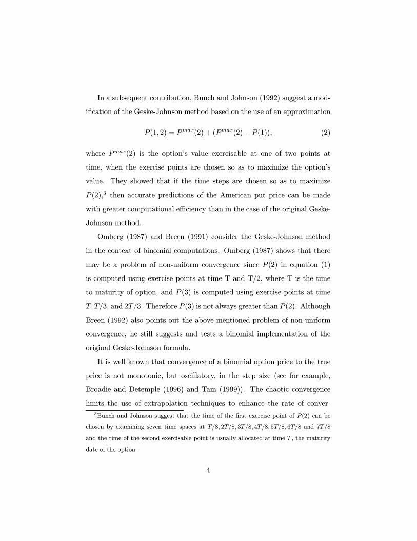
In a subsequent contribution, Bunch and Johnson (1992) suggest a mod-

ification of the Geske-Johnson method based on the use of an approximation

P (1, 2) = Pmax(2) + (Pmax(2)− P (1)), (2)

where Pmax(2) is the option’s value exercisable at one of two points at

time, when the exercise points are chosen so as to maximize the option’s

value. They showed that if the time steps are chosen so as to maximize

P (2),3 then accurate predictions of the American put price can be made

with greater computational efficiency than in the case of the original Geske-

Johnson method.

Omberg (1987) and Breen (1991) consider the Geske-Johnson method

in the context of binomial computations. Omberg (1987) shows that there

may be a problem of non-uniform convergence since P (2) in equation (1)

is computed using exercise points at time T and T/2, where T is the time

to maturity of option, and P (3) is computed using exercise points at time

T, T/3, and 2T/3. Therefore P (3) is not always greater than P (2). Although

Breen (1992) also points out the above mentioned problem of non-uniform

convergence, he still suggests and tests a binomial implementation of the

original Geske-Johnson formula.

It is well known that convergence of a binomial option price to the true

price is not monotonic, but oscillatory, in the step size (see for example,

Broadie and Detemple (1996) and Tain (1999)). The chaotic convergence

limits the use of extrapolation techniques to enhance the rate of conver-3Bunch and Johnson suggest that the time of the first exercise point of P (2) can be

chosen by examining seven time spaces at T/8, 2T/8, 3T/8, 4T/8, 5T/8, 6T/8 and 7T/8

and the time of the second exercisable point is usually allocated at time T , the maturity

date of the option.

4

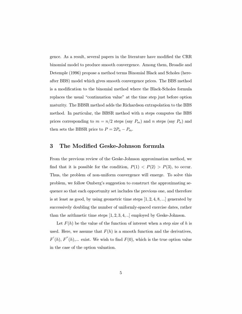
gence. As a result, several papers in the literature have modified the CRR

binomial model to produce smooth convergence. Among them, Broadie and

Detemple (1996) propose a method terms Binomial Black and Scholes (here-

after BBS) model which gives smooth convergence prices. The BBS method

is a modification to the binomial method where the Black-Scholes formula

replaces the usual “continuation value” at the time step just before option

maturity. The BBSR method adds the Richardson extrapolation to the BBS

method. In particular, the BBSR method with n steps computes the BBS

prices corresponding to m = n/2 steps (say Pm) and n steps (say Pn) and

then sets the BBSR price to P = 2Pn − Pm.

3 The Modified Geske-Johnson formula

From the previous review of the Geske-Johnson approximation method, we

find that it is possible for the condition, P (1) < P (2) > P (3), to occur.

Thus, the problem of non-uniform convergence will emerge. To solve this

problem, we follow Omberg’s suggestion to construct the approximating se-

quence so that each opportunity set includes the previous one, and therefore

is at least as good, by using geometric time steps [1, 2, 4, 8, ...] generated by

successively doubling the number of uniformly-spaced exercise dates, rather

than the arithmetic time steps [1, 2, 3, 4, ..] employed by Geske-Johnson.

Let F (h) be the value of the function of interest when a step size of h is

used. Here, we assume that F (h) is a smooth function and the derivatives,

F0(h), F

00(h),... exist. We wish to find F (0), which is the true option value

in the case of the option valuation.

5

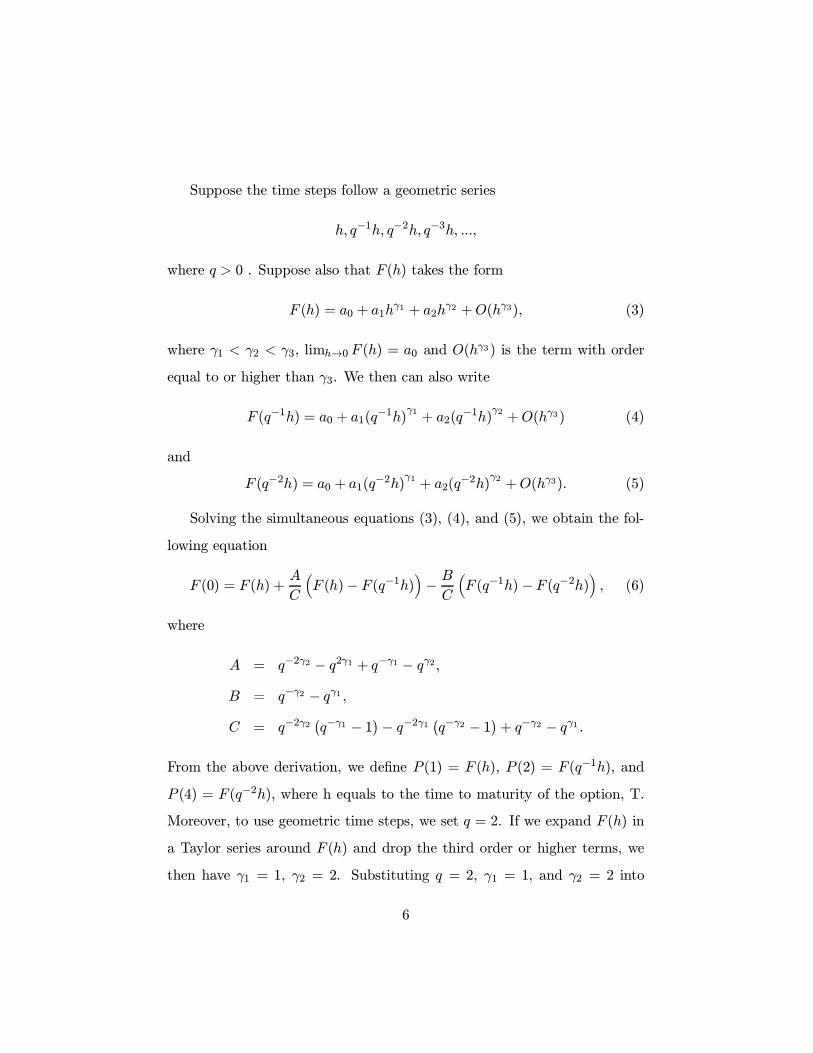
Suppose the time steps follow a geometric series

h, q−1h, q−2h, q−3h, ...,

where q > 0 . Suppose also that F (h) takes the form

F (h) = a0 + a1hγ1 + a2h

γ2 +O(hγ3), (3)

where γ1 < γ2 < γ3, limh→0 F (h) = a0 and O(hγ3) is the term with order

equal to or higher than γ3. We then can also write

F (q−1h) = a0 + a1(q−1h)γ1+ a2(q

−1h)γ2 +O(hγ3) (4)

and

F (q−2h) = a0 + a1(q−2h)γ1 + a2(q

−2h)γ2 +O(hγ3). (5)

Solving the simultaneous equations (3), (4), and (5), we obtain the fol-

lowing equation

F (0) = F (h) +A

C

³F (h)− F (q−1h)

´− BC

³F (q−1h)− F (q−2h)

´, (6)

where

A = q−2γ2 − q2γ1 + q−γ1 − qγ2,B = q−γ2 − qγ1 ,C = q−2γ2

¡q−γ1 − 1¢− q−2γ1 ¡q−γ2 − 1¢+ q−γ2 − qγ1 .

From the above derivation, we define P (1) = F (h), P (2) = F (q−1h), and

P (4) = F (q−2h), where h equals to the time to maturity of the option, T.

Moreover, to use geometric time steps, we set q = 2. If we expand F (h) in

a Taylor series around F (h) and drop the third order or higher terms, we

then have γ1 = 1, γ2 = 2. Substituting q = 2, γ1 = 1, and γ2 = 2 into

6

equation (6), we obtain the modified Geske-Johnson approximation formula

as follows:

P (1, 2, 4) = P (4) +5

3(P (4)− P (2))− 1

3(P (2)− P (1)), (7)

where P (1, 2, 4) denotes the value of the approximated American option

using the values of options with 1, 2, and 4 exercise points.

In equation (7), P (4) is the value of option exercisable at time steps

T/4, 2T/4, 3T/4, and T . Because we use a geometric time step, we can en-

sure that P (4) ≥ P (2) ≥ P (1) always holds. The reason for this is that theexercise points of P (4) include all the exercise points of P (2), while the exer-

cise points of P (2) include all the exercise points of P (1). Thus, the modified

Geske-Johnson formula is able to overcome the shortcomings of non-uniform

convergence encountered in the original Geske-Johnson formula.

4 The Repeated Richardson Extrapolation Tech-

nique for Predicting the Intervals of American

Option Values

We now turn to the question of how to predict the interval of true option

values when the Breen and modified Breen AB models are used to value

American-style options. To derive the predicted interval of the true option

values, we have to employ a numerical method, the repeated Richardson

extrapolation. A repeated Richardson extrapolation will get the same re-

sults as those of polynomial Richardson extrapolation methods when the

7

same expansion of the truncation error is used.4 The advantage to using a

repeated Richardson extrapolation is that we can predict the interval of the

true option values.

As stated earlier, the Breen AB model uses arithmetic time steps to

get the approximation formula with polynomial Richardson extrapolation,

while the modified Breen AB model uses geometric time steps. In this

section we establish an algorithm that can be used by repeated Richardson

extrapolation no matter what kind of time steps are used.

Often in numerical analysis, an unknown quantity, a0,(the same con-

cept as the value of American options in our case), is approximated by

a calculable function, F (h), depending on a parameter h > 0, such that

F (0) = limh→0 F (h) = a0. If we know the complete expansion of the

truncation error about function F (h), then we can perform the repeated

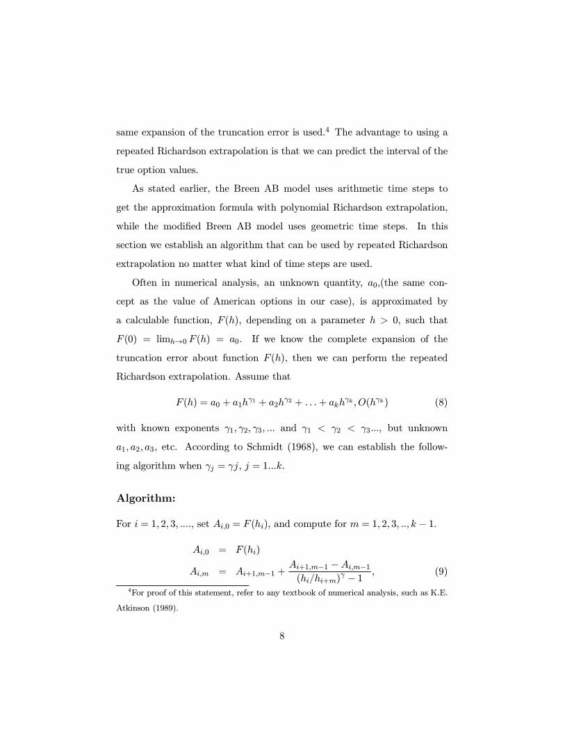
Richardson extrapolation. Assume that

F (h) = a0 + a1hγ1 + a2h

γ2 + . . .+ akhγk , O(hγk) (8)

with known exponents γ1, γ2, γ3, ... and γ1 < γ2 < γ3..., but unknown

a1, a2, a3, etc. According to Schmidt (1968), we can establish the follow-

ing algorithm when γj = γj, j = 1...k.

Algorithm:

For i = 1, 2, 3, ...., set Ai,0 = F (hi), and compute for m = 1, 2, 3, .., k − 1.

Ai,0 = F (hi)

Ai,m = Ai+1,m−1 +Ai+1,m−1 −Ai,m−1(hi/hi+m)

γ − 1 , (9)

4For proof of this statement, refer to any textbook of numerical analysis, such as K.E.

Atkinson (1989).

8

where m is the repeated times when the repeated Richardson extrapola-

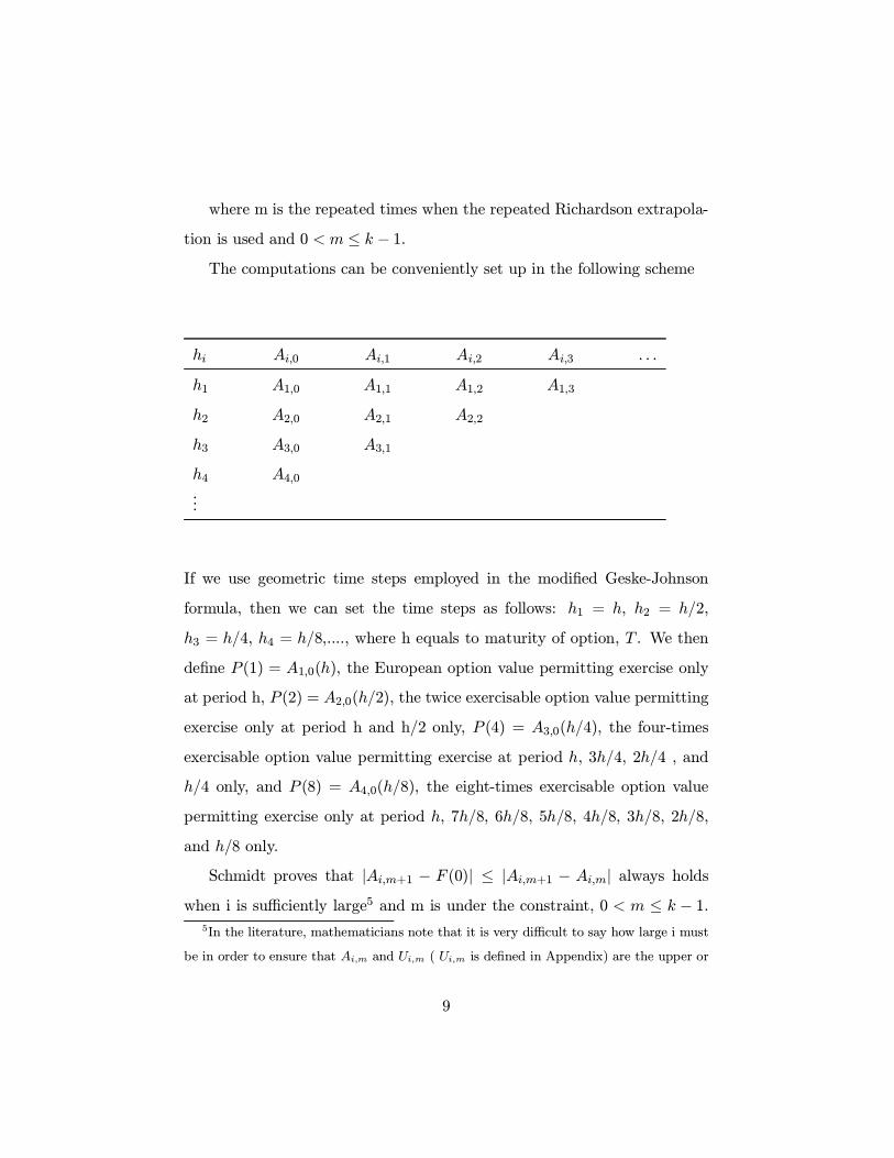
tion is used and 0 < m ≤ k − 1.The computations can be conveniently set up in the following scheme

hi Ai,0 Ai,1 Ai,2 Ai,3 . . .

h1 A1,0 A1,1 A1,2 A1,3

h2 A2,0 A2,1 A2,2

h3 A3,0 A3,1

h4 A4,0...

If we use geometric time steps employed in the modified Geske-Johnson

formula, then we can set the time steps as follows: h1 = h, h2 = h/2,

h3 = h/4, h4 = h/8,...., where h equals to maturity of option, T . We then

define P (1) = A1,0(h), the European option value permitting exercise only

at period h, P (2) = A2,0(h/2), the twice exercisable option value permitting

exercise only at period h and h/2 only, P (4) = A3,0(h/4), the four-times

exercisable option value permitting exercise at period h, 3h/4, 2h/4 , and

h/4 only, and P (8) = A4,0(h/8), the eight-times exercisable option value

permitting exercise only at period h, 7h/8, 6h/8, 5h/8, 4h/8, 3h/8, 2h/8,

and h/8 only.

Schmidt proves that |Ai,m+1 − F (0)| ≤ |Ai,m+1 − Ai,m| always holdswhen i is sufficiently large5 and m is under the constraint, 0 < m ≤ k − 1.

5In the literature, mathematicians note that it is very difficult to say how large i must

be in order to ensure that Ai,m and Ui,m ( Ui,m is defined in Appendix) are the upper or

9

6 Here, F(0) is the true American option value when the repeated Richard-

son extrapolation is used to approximate the American-style option values.

Thus, we are able to predict the interval of the allocation of the true op-

tion values by setting a desired accurate criterion according to the above

inequality. We will show, by simulation, how to predict the interval of the

true option values by using the repeated Richardson extrapolation. It is very

easy to prove that, in the case of using geometric time steps, the two times

repeated Richardson method will yield the same formula as the modified

Geske-Johnson formula.7

5 Numerical Analysis

5.1 Computational Efficiency and Accuracy

In this section we use the modified Geske-Johnson formula in the context

of accelerated binomial computations, termed as the modified Breen AB

model, to show the accuracy and efficiency of our method. To compare the

computational accuracy of the Breen AB model with that of the modified

lower bound of F (0). However, they suggest that, for practical purpose, the extrapolation

should be stopped “if a finite number of Ai,m and Ui,m decrease or increase monotonically,

and if |Ai,m−Ui,m| is small enough for accuracy.” Apart from using the above suggestion

to test the data in tables 1 and 2, from Tables 6 and 7 we found out that when i=2 and

m=1, m=2, or m=3, there are only a very low percentage violate the inequality. However,

the violation of error boundaries is not very significant. Thus, we can ignore them.

6The proof of this inequality is presented in the Appendix according to Schmidt (1968).7In the case of geometric time steps, we can also prove that the three points (four

points) polynomial Richardson extrapolation will yield the same results as those of two-

times (three-times) repeated Richardson extrapolation. The proofs are available on request

to the authors.

10

Breen AB model, we use the CRR model as a benchmark. All the binomial

trees are at the time steps of 996.

From Tables 1 and 2 we find that the modified Breen AB model almost

always dominates the Breen AB model with only two exceptions. Both the

Breen and the modified Breen AB models can approximate the values of

American put options to a high degree of accuracy. The pricing errors range

from one to two cents far less than the transaction cost. The results are not

surprising at all since the modified Breen AB model using the value of P (4)

has more exercise information than the Breen’s AB model using the value

of P (3). This result illustrates that the modified Breen AB model can not

only solve the problem of non-uniform convergence, but also improve the

computational accuracy of Breen’s AB model.

The benefit of using the various AB models to value American-style

options is able to reduce the numbers of node calculations. Thus, the AB

model can significantly improve the computational efficiency. The total

number of node calculations for the CRR binomial model, Breen’s ABmodel,

and the modified Breen’s AB mode are (n + 1)2, 4n + 10, and 4.5n + 11,

respectively. Surprising the modified Breen AB model only need a little

more node calculation than those of the Breen AB model. The reason for

this achievement is that P (2) and P (4) in the modified Breen AB model

have common time period T/2, whereas P (2) and P (3) in the Breen AB

model do not have a common time period. In terms of CPU time for an

option’s computation, the modified Breen’s AB model is as fast as Breen’s

AB model. However, both the Breen and modified Breen AB models are far

more computationally efficient than the CRR binomial model.

11

5.2 The Accuracy of the BBSMethod with Repeated Richard-

son Extrapolation Techniques

In this subsection we investigate the possibility of combining the BBSmethod

with the repeated Richardson extrapolation technique. We apply the BBS

method with a repeated Richardson extrapolation in number of time steps to

price European options, because the true prices are easily to calculate. The

root-mean-squared (hereafter RMS) relative error is used as the measure of

accuracy. The RMS error is defined by

RMS =

vuut 1

m

mXi=1

ei2, (10)

where ei = (P ∗i − Pi)/Pi is the relative error, Pi is the true option price(Black-Scholes), and P ∗i is the estimated option price obtained from the

BBS Method with repeated Richardson Extrapolation Techniques.

Many points can be drawn from Table 3. First, it is clear from the third

column of Table 3 that the pricing error of an N-step BBSmodel for standard

options is at the rate of O(1/N). In contrast, Heston and Zhou (2000) show

that the pricing error of an N-step CRR model fluctuates between the rate of

O(1/√N) and O(1/N). As a result, the BBSR method with geometric time

steps produces very accurate prices for European options (see the fourth

column of Panel B in Table 3). Second, the pricing errors from geometric

time steps are far smaller than that of arithmetic time steps. Third, Table

3 reveals that the repeated Richardson extrapolation in time steps cannot

further improve the accuracy. For example, Panel B shows that the pricing

error of A4,1 (obtained from a two-point Richardson extrapolation of BBS

prices with 160 and 320 steps) is actually smaller than that of A3,2 (obtained

from a three-point Richardson extrapolation of BBS prices with 80, 160, and

12

320 steps). Therefore, in the rest of the numerical evaluations we apply only

two-point Richardson extrapolation of BBS prices with N/2 and N steps.

5.3 The Predicted Intervals of the True American Option’s

values Using Repeated Richardson Extrapolation Tech-

niques

To choose the benchmark method for calculating the true values of American

options, we compare the accuracy of the CRR and BBSR models when both

methods are applied to price European options. It is clear from Table 4

that the RMS relative error of the BBSR method is far smaller than that

of the CRR method. Our result is consistent with the findings of Broadie

and Detemple (1996). Therefore, we will use the BBSR method with 10800

steps to calculate benchmark prices of American options.

We now turn to compare the accuracy of the Richardson extrapolation

for the number of exercisable points to estimate American option values.

Both arithmetic and geometric exercisable times are examined. In Table

5 the true values of all options are estimated by the BBSR method with

10, 800 steps. The results indicate that the pricing errors of geometric ex-

ercisable times are smaller than that of arithmetic exercisable times. This

finding supports the finding that a Richardson extrapolation with geometric

exercisable times can avoid the problem of non-uniform convergence. More-

over, the repeated Richardson extrapolation technique can further reduce

the pricing errors. In other words, an (n+ 1)-point Richardson extrapola-

tion generally produces more accurate prices than an n-point Richardson

extrapolation. For example, Panel B shows that the RMS relative errors of

A1,2 (obtained from a three-point Richardson extrapolation of P (1), P (2),

13

and P (4)) is 0.346 %, which is smaller than that (0.427 %) of A2,1 (obtained

from a two-point Richardson extrapolation of P (2) and P (4)).

One specific advantage of the repeated Richardson extrapolation is that

it allows us to specify the accuracy of an approximation to the unknown true

option price. That is, the Schmidt inequality can be used to predict tight

bounds (with desired tolerable errors) of the true option values. We test the

validity of the Schmidt inequality over 243 options for both arithmetic and

geometric exercisable times in Tables 6 and 7. The denominator represents

the number of option price estimates that match |Ai,m+1 − F (0)| < the

desired errors, and the numerator is the number of option price estimates

that match |Ai,m+1 − F (0)| < the desired errors and |Ai,m+1 −Ai,m| < thedesired errors.

The results in Tables 6 and 7 indicate that increasing i or m will increase

the number of price estimates with errors less than the desired accuracy. It is

also clear that the Schmidt inequality is seldom violated especially when i or

m is large (i = 3, 4 andm = 2, 3). For example, when i= m=2, 228 out of 243

option price estimates have errors smaller than 0.2% of the European option

value, and 225 out of 228 option price estimates satisfy Schmidt inequality.

Moreover, the findings support that the repeated Richardson extrapolation

with geometric exercisable times works better than with arithmetic exercis-

able times. This confirms the previous result that a Richardson extrapola-

tion with geometric exercisable times can avoid the problem of non-uniform

convergence.

14

6 Conclusion and Suggestion

In this paper we re-examine the original Geske-Johnson formula. We then

extend the analysis by deriving a modified Geske-Johnson formula which

is able to overcome the possibility of non-uniform convergence encountered

in the original Geske-Johnson formula. Another contribution of this paper

is that we propose a numerical method which can estimate the predicted

intervals of the true option values when the accelerated binomial option

pricing models are used to value the American-style options.

The findings are summarized as follows: (i) The modified Breen AB

model is as fast as the Breen AB model, whereas both the Breen and mod-

ified Breen AB model are faster than the CRR binomial model. However,

on average the modified Breen AB model performs better than the Breen

model for valuing American-style put options with a range of exercise prices.

More importantly the modified Breen AB model can overcome the drawback

from possible non-uniform convergence in the Breen AB model. Therefore,

we recommend replacing the Breen AB model with the modified Breen AB

model for the valuation of American-style put options. (ii) The Richard-

son extrapolation approach can improve the computational accuracy for the

BBS method proposed by Broadie and Detemple (1996), while the repeated

Richardson extrapolation technique cannot. (iii) Using Schmidt’s inequal-

ity, we are able to obtain the intervals of the true American option values.

This helps to specify the accuracy of an approximation to the unknown true

option price and to determine the smallest value of n that can solely be used

in an option price approximation. This research article is the first to discuss

how to get the predicted intervals of the true option values in the literature

15

of finance. We believe that the repeated Richardson method will be very

useful for practitioners to predict the intervals of the true option values.

The advantage in using the accelerated binomial option pricing model is

its ability to reduce tremendous amounts of node calculations. It is especially

useful to calculate the prices of options where n is relatively large, or where

more than one variable affects the option’s value. We will leave the above-

mentioned potential applications to future research.

16

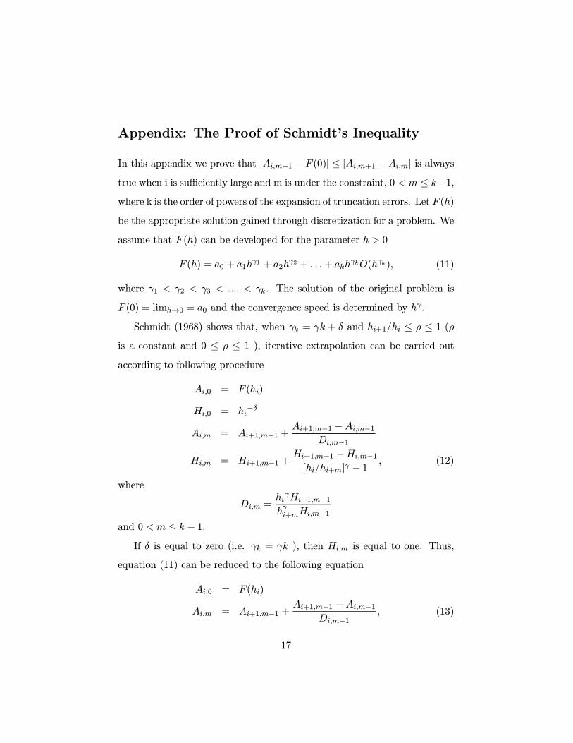
Appendix: The Proof of Schmidt’s Inequality

In this appendix we prove that |Ai,m+1 − F (0)| ≤ |Ai,m+1 −Ai,m| is alwaystrue when i is sufficiently large and m is under the constraint, 0 < m ≤ k−1,where k is the order of powers of the expansion of truncation errors. Let F (h)

be the appropriate solution gained through discretization for a problem. We

assume that F (h) can be developed for the parameter h > 0

F (h) = a0 + a1hγ1 + a2h

γ2 + . . .+ akhγkO(hγk), (11)

where γ1 < γ2 < γ3 < .... < γk. The solution of the original problem is

F (0) = limh→0 = a0 and the convergence speed is determined by hγ .

Schmidt (1968) shows that, when γk = γk + δ and hi+1/hi ≤ ρ ≤ 1 (ρis a constant and 0 ≤ ρ ≤ 1 ), iterative extrapolation can be carried outaccording to following procedure

Ai,0 = F (hi)

Hi,0 = hi−δ

Ai,m = Ai+1,m−1 +Ai+1,m−1 −Ai,m−1

Di,m−1

Hi,m = Hi+1,m−1 +Hi+1,m−1 −Hi,m−1[hi/hi+m]γ − 1 , (12)

where

Di,m =hiγHi+1,m−1

hγi+mHi,m−1

and 0 < m ≤ k − 1.If δ is equal to zero (i.e. γk = γk ), then Hi,m is equal to one. Thus,

equation (11) can be reduced to the following equation

Ai,0 = F (hi)

Ai,m = Ai+1,m−1 +Ai+1,m−1 −Ai,m−1

Di,m−1, (13)

17

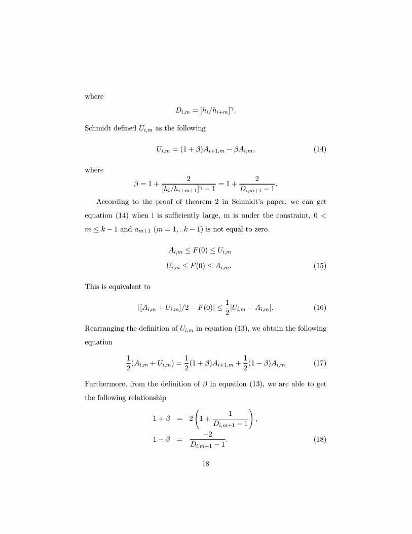
where

Di,m = [hi/hi+m]γ .

Schmidt defined Ui,m as the following

Ui,m = (1+ β)Ai+1,m − βAi,m, (14)

where

β = 1 +2

[hi/hi+m+1]γ − 1 = 1 +2

Di,m+1 − 1 .

According to the proof of theorem 2 in Schmidt’s paper, we can get

equation (14) when i is sufficiently large, m is under the constraint, 0 <

m ≤ k − 1 and am+1 (m = 1, ..k − 1) is not equal to zero.

Ai,m ≤ F (0) ≤ Ui,mUi,m ≤ F (0) ≤ Ai,m. (15)

This is equivalent to

|[Ai,m +Ui,m]/2− F (0)| ≤ 12|Ui,m −Ai,m|. (16)

Rearranging the definition of Ui,m in equation (13), we obtain the following

equation

1

2(Ai,m + Ui,m) =

1

2(1 + β)Ai+1,m +

1

2(1− β)Ai,m (17)

Furthermore, from the definition of β in equation (13), we are able to get

the following relationship

1 + β = 2

Ã1 +

1

Di,m+1 − 1

!,

1− β =−2

Di,m+1 − 1 . (18)

18

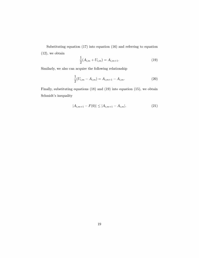
Substituting equation (17) into equation (16) and referring to equation

(12), we obtain1

2(Ai,m +Ui,m) = Ai,m+1. (19)

Similarly, we also can acquire the following relationship

1

2(Ui,m −Ai,m) = Ai,m+1 −Ai,m. (20)

Finally, substituting equations (18) and (19) into equation (15), we obtain

Schmidt’s inequality

|Ai,m+1 − F (0)| ≤ |Ai,m+1 −Ai,m|. (21)

19

References

Atkinson, K.E. (1989), An Introduction to Numerical Analysis, 2nd Edition,

John Wiley & Sons, Inc. New York.

Barone-Adesi, G. and R.E. Whaley. (1987), “Efficient Analytic Approxima-

tion of American Option Values,” Journal of Finance, 42, June, 301-320.

Breen, R. (1991), “The Accelerated Binomial Option Pricing Model,” Jour-

nal of Financial and Quantitative Analysis, 26, June, 153-164.

Broadie, M. and J.B. Detemple, 1996, American Option Valuation: New

Bounds, Approximations, and a Comparison of Existing Methods, The Re-

view of Financial Studies, 9, 1211-1250.

Bunch, D.S. and Johnson (1992), “A Simple Numerically Efficient Valuation

Method for American Puts Using a Modified Geske-Johnson Approach,”

Journal of Finance, 47, June, 809-816.

Cox, J.C. and M. Rubinstein (1985), Options Markets, Prentice-Hall, En-

glewood Cliffs, New Jersey.

Cox, J.C., S.A. Ross and M Rubinstein (1979), “Option Pricing: A Simpli-

fied Approach,” Journal of Financial Economics, 7, September, 229-263.

Geske, R. and Johnson (1979), “The Valuation of Compound Options,”

Journal of Financial Economics, 7, March, 63-81.

Geske, R. and Johnson (1984), “The American Put Valued Analytically,”

Journal of Finance, 39, December, 1511-1542.

Geske, R. and Shastri, K. (1985), “Valuation by Approximation: A Com-

20

parison of Alternative Option Valuation Techniques,” Journal of Financial

and Quantitive Analysis, 20, March, 45-71.

Heston, S. and G. Zhou (2000), “On the Rate of Convergence of Discrete-

Time Contingent Claims,” Mathematical Finance, 53-75.

Ho, T.S., R.C. Stapleton and M.G. Subrahmanyam (1997), “The Valuation

of American Options with Stochastic Interest Rates: A Generalization of

the Geske-Johnson Technique,” Journal of Finance, 57, June, 827-839.

Joyce, D.C. (1971), “Survey of Extrapolation Processes in Numerical Analy-

sis,” SIAM Review , 13, 4, October, 435-483.

Omberg, E. (1987), “A Note on the Convergence of the Binomial Pricing

and Compound Option Models,” Journal of Finance, 42, June, 463-469.

Rendleman, R.J., and Bartter, B.J. (1979), “Two-State Option Pricing.”

Journal of Finance, 34, December, 1093-1110.

Shastri, K. and Tandon, K. (1986), “On the Use of EuropeanModels to Price

American Options on Foreign Currency,” The Journal of Futures Markets,

6, 1, 93-108.

Schmidt J.W. (1968) “Asymptotische Einschliebung bei Konvergenzbeschleni-

genden Verfahren. II,” Numerical Mathematics, 11, 53-56.

Stapleton, R.C. and M.G. Subrahmanyam (1984), “The Valuation of Op-

tions When Asset Returns are Generated by a Binomial Process,” Journal

of Finance, 5, 1529-1539.

Tian, Y. (1999), “A Flexible Binomial Option Pricing Model,” Journal of

Futures Markets, 817-843.

21