riemann surfaces - scuola internazionale superiore …grava/chapt1_5.pdflocally looks like an open...
TRANSCRIPT
Chapter 1
Riemann surfaces
1.1 Definition of a Riemann surface and basic examples
In its broadest sense a Riemann surface is a one dimensional complex manifold thatlocally looks like an open set of the complex plane, while its global topology can be quitedifferent from the complex plane. The main reason why Riemann surfaces are interestingis that one can speak of complex functions on a Riemann surface as much as the complexfunction on the complex plane that one encounters in complex analysis.
Elementary example of Riemann surfaces are the complex plane C, the disk
D “ tz P C, |z| ă 1u
or the upper half space
H “ tz P C, =pzq ą 0u.
B. Riemann introduced the concept of Riemann surface to make sense of multivaluedfunctions like the square root or the logarithm. For the geometric representation of multi-valued functions of a complex variable w “ wpzq it is not convenient to regard z as apoint of the complex plane. For example, take w “
?z. On the positive real semiaxis
z P R, z ą 0 the two branches w1 “ `?
z and w2 “ ´?
z of this function are welldefined by the condition w1 ą 0. This is no longer possible on the complex plane. Indeed,the two values w1, 2 of the square root of z “ r eiψ
w1 “?
r eiψ2 , w2 “ ´?
r eiψ2 “?
reiψ`2π2 , (1.1)
interchange when passing along a path
zptq “ r ei pψ`tq, t P r0, 2πs
1
2 CHAPTER 1. RIEMANN SURFACES
encircling the point z “ 0. It is possible to select a branch of the square root as a functionof z by restricting the domain of this function for example, by making a cut from zero toinfinity. Namely the function
?z is single-valued in the cut plane Czr0,`8q. Riemann’s
idea was to combine the two branches of the function?
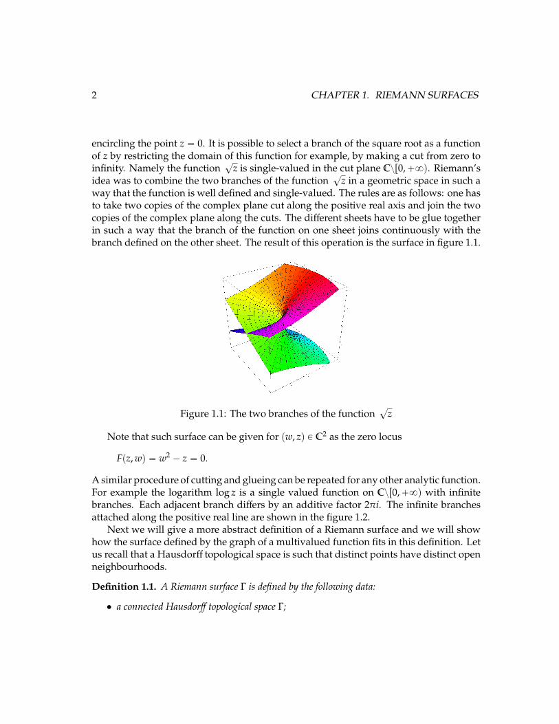
z in a geometric space in such away that the function is well defined and single-valued. The rules are as follows: one hasto take two copies of the complex plane cut along the positive real axis and join the twocopies of the complex plane along the cuts. The different sheets have to be glue togetherin such a way that the branch of the function on one sheet joins continuously with thebranch defined on the other sheet. The result of this operation is the surface in figure 1.1.
Figure 1.1: The two branches of the function?
z
Note that such surface can be given for pw, zq P C2 as the zero locus
Fpz,wq “ w2 ´ z “ 0.
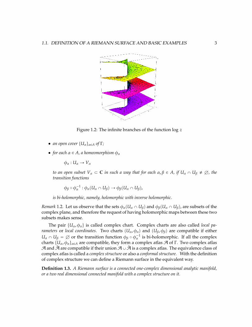
A similar procedure of cutting and glueing can be repeated for any other analytic function.For example the logarithm log z is a single valued function on Czr0,`8q with infinitebranches. Each adjacent branch differs by an additive factor 2πi. The infinite branchesattached along the positive real line are shown in the figure 1.2.
Next we will give a more abstract definition of a Riemann surface and we will showhow the surface defined by the graph of a multivalued function fits in this definition. Letus recall that a Hausdorff topological space is such that distinct points have distinct openneighbourhoods.
Definition 1.1. A Riemann surface Γ is defined by the following data:
• a connected Hausdorff topological space Γ;
1.1. DEFINITION OF A RIEMANN SURFACE AND BASIC EXAMPLES 3
Figure 1.2: The infinite branches of the function log z
• an open cover tUαuαPA of Γ;
• for each α P A, a homeomorphism φα
φα : Uα Ñ Vα
to an open subset Vα Ă C in such a way that for each α, β P A, if Uα X Uβ , H, thetransition functions
φβ ˝ φ´1α : φαpUα XUβq Ñ φβpUα XUβq,
is bi-holomorphic, namely, holomorphic with inverse holomorphic.
Remark 1.2. Let us observe that the sets φαpUα XUβq and φβpUα XUβq, are subsets of thecomplex plane, and therefore the request of having holomorphic maps between these twosubsets makes sense.
The pair tUα, φαu is called complex chart. Complex charts are also called local pa-rameters or local coordinates. Two charts pUα, φαq and pUβ, φβq are compatible if eitherUα X Uβ “ H or the transition function φβ ˝ φ´1
α is bi-holomorphic. If all the complexcharts tUα, φαuαPA are compatible, they form a complex atlasA of Γ. Two complex atlasA and A are compatible if their unionAY A is a complex atlas. The equivalence class ofcomplex atlas is called a complex structure or also a conformal structure. With the definitionof complex structure we can define a Riemann surface in the equivalent way.
Definition 1.3. A Riemann surface is a connected one-complex dimensional analytic manifold,or a two real dimensional connected manifold with a complex structure on it.
4 CHAPTER 1. RIEMANN SURFACES
Let φ and φ be two local homeomorphism from two open sets U and U of Γ withU X U ,H. Let P and P0 two points in U X U and denote by z “ φpPq and w “ φpPq thetwo local coordinates with z0 “ φpP0q and w0 “ φpP0q. Then the holomorphic transitionfunction T “ φ ˝ φ´1 must be of the form
z “ Tpwq “ Tpw0q `ÿ
ką0
akpw´ w0qk, a1 , 0 (1.2)
with holomorphic inverse
w “ T´1pzq “ T´1pz0q `ÿ
ką0
bkpz´ z0qk, b1 , 0,
namely the linear coefficient of the above Taylor expansions near the point w0 or z0 isnecessarily nonzero.
Remark 1.4. We recall that that a manifold is called orientable if it has an atlas whosetransition functions have positive Jacobian determinant. If Γ is a Riemann surface, thenthe manifold Γ is orientable. Indeed let z “ x ` iy be a local coordinate in some openneighbourhood of z0 in Γ. Another local coordinate w “ u` iv is connected with the firstby a holomorphic change of variable w “ Tpzq with w0 “ Tpz0q which thus determines asmooth change of real coordinates. We want to show that the determinant
det
¨
˚
˝
BuBx
BuBy
BvBx
BvBy
˛
‹
‚“ uxvy ´ uyvx
calculated in px0, y0q is positive. We observe that w “ wpzq is a holomorphic function of z
anddwdz|z“z0 , 0. We can use Cauchy Riemann equations ux “ vy and uy “ ´vx to write
dwdz“ ux ´ iuy and
dwdz“ ux ` iuy to conclude that
det
¨
˚
˝
BuBx
BuBy
BvBx
BvBy
˛
‹
‚
ˇ
ˇ
ˇ
ˇ
ˇ
ˇ
ˇ x“x0y“y0
“ pu2x ` u2
yq| x“x0y“y0“
ˇ
ˇ
ˇ
ˇ
dwdz
ˇ
ˇ
ˇ
ˇ
2
z“z0
ą 0.
Example 1.5. Elementary examples of Riemann surfaces
(a) The complex plane C. The complex atlas is define by one chart that is C itself withthe identity map.
1.1. DEFINITION OF A RIEMANN SURFACE AND BASIC EXAMPLES 5
(b) The extended complex plane C “ C Y 8, namely the complex plane C with oneextra point8. We make C into a Riemann surface with an atlas with two charts:
U1 “ C
U2 “ Czt0u,
with φ1 the identity map and
φ2pzq “"
1z, for z P Czt0u0, for z “ 8.
1.1.1 Affine plane curves
Let us consider a polynomial Fpz,wq “řn
i“1 aipzqwi of two complex variables z and w.The zero set Fpz,wq defines a n-valued function w “ wpzq. The basic idea of Riemannsurface theory is to replace the domain of the function wpzq by its graph
Γ :“ tpz,wq P C2 | Fpz,wq “nÿ
i“0
aipzqwn´i “ 0u (1.3)
and to study the function w as a single-valued function on Γ rather then a multivaluedfunction of z. As in the example of
?z, the multivalued function w “ wpzq “
?z becomes
a single-valued function w “ wpPq of a point P of the algebraic surface Γ: if P “ pz,wq P Γ,then wpPq “ w (the projection of the graph on the the w-axis). From the real point ofview the algebraic curve (1.3) is a two-dimensional surface in C2 “ R4 given by the twoequations
<Fpz,wq “ 0=Fpz,wq “ 0
*
.
In the theory of functions of a complex variable one encounters also more complicated(nonalgebraic) curves, where Fpz,wq is not a polynomial. For example, the equationew´ z “ 0 determines the surface of the logarithm or sin w´ z “ 0 determines the surfaceof the arcsin. Such surfaces will not be considered here.
Definition 1.6. An affine plane curve Γ is a subset in C2 defined by the equation (1.3 ) whereFpz,wq is polynomial in z and w. The curve Γ is nonsingular if for any point P0 “ pz0,w0q P Γthe complex gradient vector
gradCF|P0 “
ˆ
BFpz,wqBz
,BFpz,wqBw
˙ˇ
ˇ
ˇ
ˇ
pz“z0,w“w0q
does not vanish. If the polynomial Fpz,wq is irreducible, the curve Γ is called irreducible affineplane curve.
6 CHAPTER 1. RIEMANN SURFACES
Remark 1.7. A non trivial theorem states that an irreducible affine plane curve is connected(see Theorem 8.9 in O. Forster, Lectures on Riemann surfaces, Springer Verlag 1981).
In order to define a complex structure on Γ we need the following complex version ofthe implicit function theorem.
Lemma 1.8. [Complex implicit function theorem] Let Fpz,wq be an analytic function of thevariables z and w in a neighborhood of the point P0 “ pz0,w0q such that Fpz0,w0q “ 0 andBwFpz0,w0q , 0. Then there exists a unique function φpzq such that Fpz, φpzqq “ 0 andφpz0q “ w0. This function is analytic in z in some neighborhood of z0.
Proof. Let z “ x ` iy and w “ u ` iv, F “ f ` ig. Then the equation Fpz,wq “ 0 can bewritten as the system
"
f px, y,u, vq “ 0gpx, y,u, vq “ 0 (1.4)
The condition of the real implicit function theorem are satisfied for this system: the matrix
¨
˚
˚
˚
˝
B fBu
B fBv
BgBu
BgBv
˛
‹
‹
‹
‚
pz0,w0q
is nonsingular because
det
¨
˚
˚
˚
˝
B fBu
B fBv
BgBu
BgBv
˛
‹
‹
‹
‚
“
ˇ
ˇ
ˇ
ˇ
BFBw
ˇ
ˇ
ˇ
ˇ
2
ą 0,
( we use only the analyticity in w of the function Fpz,wq). Thus, in some neighbourhood ofpz0,w0q there exist a smooth functionφpz, zq “ φ1px, yq`iφ2px, yq such that Fpz, φpz, zqq “ 0,with φpz0, z0q “ w0. Differentiating with respect to z
0 “ddz
Fpz, φpz, zqq “ Fwddzφpz, zq.
Since Fw , 0, the above relation implies thatddzφpz, zq “ 0 which shows that φpzq is an
analytic function of z.
1.1. DEFINITION OF A RIEMANN SURFACE AND BASIC EXAMPLES 7
Remark 1.9. A constructive way of obtaining the function φpzq is to apply the ResidueTheorem. Indeed let us consider the function Fpz,wq where z is treated as a parameter.Let D0 be a small disk around w0 where Fpz0,w0q “ 0 and Fwpz0,wq|w“w0 , 0. Then thenumber of solutions of the equation Fpz0,wq “ 0 counted with multiplicity is given by theintegral
12πi
ż
BD0
Fwpz0,wqFpz0,wq
dw,
where BD0 is the boundary of D0. We assume D0 sufficiently small so that the equationFpz0,wq “ 0 has only the solution w0 in the closure of D0. Then the above integral is equalto one. Furthermore by the residue theorem one has
12πi
ż
BD0
wFwpz0,wqFpz0,wq
dw “ w0.
By continuity, for z sufficiently close to z0 there is a disk D centred at w such that theequation Fpz,wq “ 0 has only one solution w “ φpzq in the closure of D and
12πi
ż
BDw
Fwpz,wqFpz,wq
dw “ φpzq,
where φpz0q “ z0 and Fpz, φpzqq “ 0. Clearly the function φpzq is an analytic function of z.
Theorem 1.10. Let Γ be an irreducible affine plane curve defined in (1.3). If Γ is non singular,then Γ is a Riemann surface.
Proof. Γ is connected since Fpz,wq is irreducible. Let us define a complex structure on Γ.Let P0 “ pz0,w0q be a nonsingular point of the surface Γ. Suppose, for example, that the
derivativeBFBw
is nonzero at this point. Then by the lemma 1.8, in a neighborhood U0 ofthe point P0, the surface Γ admits a parametric representation of the form
pz,wpzqq P U0 Ă Γ, wpz0q “ w0, (1.5)
where the function wpzq is holomorphic. Therefore, in this case z is a complex localcoordinate also called local parameter on Γ in a neighborhood U0 of P0 “ pz0,w0q P Γ. Forthis kind of local coordinate, the transition function is the identity.
Similarly, if the derivativeBFBz
is nonzero at the point P0 “ pz0,w0q, then we cantake w as a local parameter (an obvious variant of the lemma), and the surface Γ can berepresented in a neighborhood U0 of the point P0 in the parametric form
pzpwq,wq P Γ, zpw0q “ z0, (1.6)
8 CHAPTER 1. RIEMANN SURFACES
where the function zpwq is, of course, holomorphic. For a local parameter of this secondkind the transition function is the identity map. For a nonsingular surface it is possible touse both ways for representing the surface on the intersection of domains of the first and
second types, i.e., at points of Γ whereBFBw, 0 and
BFBz, 0 simultaneously. The resulting
transition functions w “ wpzq and, z “ zpwq are holomorphic and invertible.
The preceding arguments show that such Riemann surfaces are complex manifolds(with complex dimension 1).
Let us consider a Riemann surface Γ defined in C2 by a monic polynomial
Fpz,wq “ wn ` a1pzqwn´1 ` ¨ ¨ ¨ ` anpzq “ 0. (1.7)
Here the a1pzq, . . . , anpzq are polynomials in z. This Riemann surface is realized as ann-sheeted covering of the z-plane. The precise meaning of this is as follows: let π : Γ Ñ Cbe the projection of the Riemann surface onto the z-plane given by the formula
πpz,wq “ z. (1.8)
Then for almost all z the preimage π´1pzq consists of n distinct points
pz,w1pzqq, pz,w2pzqq, , . . . pz,wnpzqq, (1.9)
of the surface Γ where w1pzq, . . . ,wnpzq are the n roots of (1.7) for given value of z. Forcertain values of z, some of the points of the preimage can merge. This happens at thebranch points pz0,w0q of the Riemann surface where the partial derivative Fwpz,wq vanishes(recall that we consider only nonsingular curves so far).
If z0 is a branch point then the polynomial Fpz0,wq has multiple roots. The multipleroots can be determined from the system
Fpz0,wq “ 0Fwpz0,wq “ 0
*
. (1.10)
The ramification points on the z-plane can be determined, therefore, as the zeros of theresultant of Fpz,wq and Fwpz,wq and denoted by RpF,Fwqpzq. Such quantity is also calledthe discriminant of Fpz,wqwith respect to w.
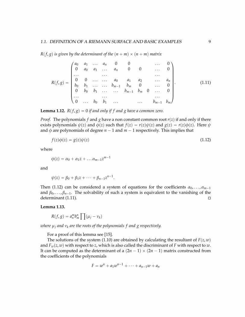
Definition 1.11. Let f pzq “ a0 ` a1z ` ¨ ¨ ¨ ` anzn and gpzq “ b0 ` b1z ` ¨ ¨ ¨ ` bmzm be twopolynomials of degree n and m respectively with ai, b j P C with an , 0 and bm , 0. The resultant
1.1. DEFINITION OF A RIEMANN SURFACE AND BASIC EXAMPLES 9
Rp f , gq is given by the determinant of the pn`mq ˆ pn`mq matrix
Rp f , gq “
¨
˚
˚
˚
˚
˚
˚
˚
˚
˚
˚
˝
a0 a1 . . . an 0 0 . . . 00 a0 a1 . . . an 0 0 . . . 0. . . . . . . . .0 0 . . . . . . a0 a1 a2 . . . anb0 b1 . . . . . . bm´1 bm 0 . . . 00 b0 b1 . . . . . . bm´1 bm 0 . . . 0. . . . . . . . .0 . . . b0 b1 . . . . . . bm´1 bm
˛
‹
‹
‹
‹
‹
‹
‹
‹
‹
‹
‚
. (1.11)
Lemma 1.12. Rp f , gq “ 0 if and only if f and g have a common zero.
Proof. The polynomials f and g have a non constant common root rpzq if and only if thereexists polynomials ψpzq and φpzq such that f pzq “ rpzqψpzq and gpzq “ rpzqφpzq. Here ψand φ are polynomials of degree n´ 1 and m´ 1 respectively. This implies that
f pzqφpzq “ gpzqψpzq (1.12)
where
φpzq “ α0 ` α1z` . . . αm´1zm´1
and
ψpzq “ β0 ` β1z` ¨ ¨ ¨ ` βn´1zn´1.
Then (1.12) can be considered a system of equations for the coefficients α0, . . . , αm´1and β0, . . . , βn´1. The solvability of such a system is equivalent to the vanishing of thedeterminant (1.11).
Lemma 1.13.
Rp f , gq “ amn bn
m
ź
pµ j ´ νkq
where µ j and νk are the roots of the polynomials f and g respectively.
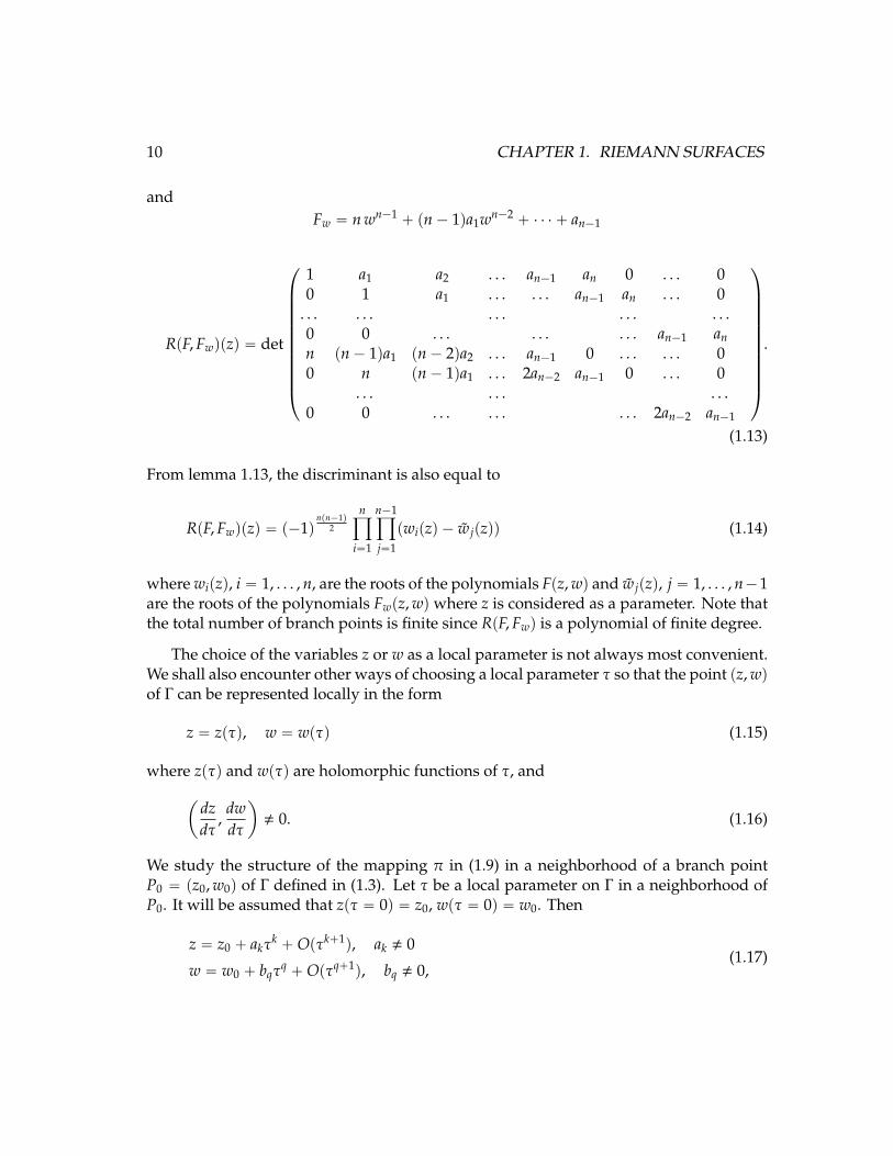
For a proof of this lemma see [15].The solutions of the system (1.10) are obtained by calculating the resultant of Fpz,wq
and Fwpz,wqwith respect to z, which is also called the discriminant of F with respect to w.It can be computed as the determinant of a p2n ´ 1q ˆ p2n ´ 1q matrix constructed fromthe coefficients of the polynomials
F “ wn ` a1wn´1 ` ¨ ¨ ¨ ` an´1w` an
10 CHAPTER 1. RIEMANN SURFACES
andFw “ n wn´1 ` pn´ 1qa1wn´2 ` ¨ ¨ ¨ ` an´1
RpF,Fwqpzq “ det
¨
˚
˚
˚
˚
˚
˚
˚
˚
˚
˚
˝
1 a1 a2 . . . an´1 an 0 . . . 00 1 a1 . . . . . . an´1 an . . . 0. . . . . . . . . . . . . . .0 0 . . . . . . . . . an´1 ann pn´ 1qa1 pn´ 2qa2 . . . an´1 0 . . . . . . 00 n pn´ 1qa1 . . . 2an´2 an´1 0 . . . 0
. . . . . . . . .0 0 . . . . . . . . . 2an´2 an´1
˛
‹
‹
‹
‹
‹
‹
‹
‹
‹
‹
‚
.
(1.13)
From lemma 1.13, the discriminant is also equal to
RpF,Fwqpzq “ p´1qnpn´1q
2
nź
i“1
n´1ź
j“1
pwipzq ´ w jpzqq (1.14)
where wipzq, i “ 1, . . . ,n, are the roots of the polynomials Fpz,wq and w jpzq, j “ 1, . . . ,n´1are the roots of the polynomials Fwpz,wq where z is considered as a parameter. Note thatthe total number of branch points is finite since RpF,Fwq is a polynomial of finite degree.
The choice of the variables z or w as a local parameter is not always most convenient.We shall also encounter other ways of choosing a local parameter τ so that the point pz,wqof Γ can be represented locally in the form
z “ zpτq, w “ wpτq (1.15)
where zpτq and wpτq are holomorphic functions of τ, and
ˆ
dzdτ,
dwdτ
˙
, 0. (1.16)
We study the structure of the mapping π in (1.9) in a neighborhood of a branch pointP0 “ pz0,w0q of Γ defined in (1.3). Let τ be a local parameter on Γ in a neighborhood ofP0. It will be assumed that zpτ “ 0q “ z0, wpτ “ 0q “ w0. Then
z “ z0 ` akτk `Opτk`1q, ak , 0
w “ w0 ` bqτq `Opτq`1q, bq , 0,
(1.17)
1.1. DEFINITION OF A RIEMANN SURFACE AND BASIC EXAMPLES 11
where ak and bq are nonzero coefficients. Since w can be taken as the local parameterin a neighborhood of P0 it follows that q “ 1. We get the form of the surface Γ in aneighborhood of a branch point:
z “ z0 ` akτk `Opτk`1q,
w “ w0 ` b1τ`Opτ2q,(1.18)
where k ą 1.
Definition 1.14. The number bzpPq “ k´ 1 is called the multiplicity of the branch point, or thebranching index of this point with respect to the projection pz,wq Ñ z.
Exercise 1.15: Let P0 “ pz0,w0q be a branch point for the curve (1.7) with respect to theprojection pz,wq Ñ z. Suppose that the local parameter in the neighbourhood of P0 is ofthe form (1.18) with k ą 1. Show that
d jFpz,wqdw j
ˇ
ˇ
ˇ
ˇ
ˇ
pz0,w0q
“ 0, j “ 0, . . . , k´ 1.
Lemma 1.16. Let pz0,w0q be a branch point of a Riemann surface Γ defined in (1.3) with respectto the projection pz,wq Ñ z. Then there exists a positive integer k ą 1 and k functions w1pzq, . . . ,wkpzq analytic on a sector Sρ,φ of the punctured disc
0 ă |z´ z0| ă ρ, argpz´ z0q ă φ
for sufficiently small ρ and any positive φ ă 2π such that
Fpz,w jpzqq ” 0 for z P Sρ,φ, j “ 1, . . . , k.
The functions w1pzq, . . . , wkpzq are continuous in the closure Sρ,φ and
w1pz0q “ ¨ ¨ ¨ “ wkpz0q “ w0.
Proof. By the nonsingularity assumption Fzpz0,w0q , 0. So the complex curve Fpz,wq “ 0can be locally parametrized in the form z “ zpwq where the analytic function zpwq isuniquely determined by the condition zpw0q “ z0. Consider the first nontrivial term ofthe Taylor expansion of this function
zpwq “ z0 ` αkpw´ w0qk ` αk`1pw´ w0q
k`1 ` . . . , k ą 1, αk , 0.
Introduce an auxiliary function
f pwq “ βpw´ w0q
„
1`αk`1
αkpw´ w0q `O
`
pw´ w0q2˘
1k
“ βpw´ w0q
„
1`αk`1
kαkpw´ w0q `O
`
pw´ w0q2˘
12 CHAPTER 1. RIEMANN SURFACES
where the complex number β is chosen in such a way that βk “ αk. The function f pwqis analytic for sufficiently small |w ´ w0|. Observe that f 1pw0q “ β , 0. Therefore theanalytic inverse function f´1 locally exists. The needed k functions w1pzq, . . . , wkpzq canbe constructed as follows
w jpzq “ f´1´
e2πi p j´1q
k pz´ z0q1k¯
, j “ 1, . . . , k (1.19)
where we choose an arbitrary branch of the k-th root of pz´ z0q for z P Sρ,φ.
Example 1.17. Elliptic and hyperelliptic Riemann surfaces have the form
Γ “ tpz,wq P C2 |w2 “ Pnpzqu, (1.20)
where Pnpzq is a polynomial of degree n. These surfaces are two-sheeted coverings of thez-plane. Here Fpz,wq “ w2 ´ Pnpzq. The gradient vector gradCF “ p´P1npzq, 2wq. A pointpz0,w0q P Γ is singular if
w0 “ 0, P1npz0q “ 0. (1.21)
Together with the condition (1.20) for a point pz0,w0q to belong to Γ we get that
Pnpz0q “ 0, P1npz0q “ 0, (1.22)
i.e. z0 is a multiple root of the polynomial Pnpzq. Accordingly, the surface (1.20) isnonsingular if and only if the polynomial Pnpzq does not have multiple roots:
Pnpzq “nź
i“1
pz´ ziq, zi , z j, for i , j. (1.23)
The curve Γ is called an elliptic curve for n “ 3, 4 and it is called hyperelliptic for n ą 4.We find the branch points of the surface (1.20). To determine them we have the system
w2 “ Pnpzq, w “ 0,
which gives us n branch points Pi “ pz “ zi,w “ 0q, i “ 1, . . . ,n. All the branch pointshave multiplicity one. In a neighborhood of any point of Γ that is not a branch point it isnatural to take z as a local parameter, and w “
a
Pnpzq is a holomorphic function. In aneighborhood of a branch point Pi it is convenient to take
τ “?
z´ zi, (1.24)
1.1. DEFINITION OF A RIEMANN SURFACE AND BASIC EXAMPLES 13
as a local parameter. Then for points of the Riemann surface (1.20) we get the localparametric representation
z “ zi ` τ2, w “ τ
d
ź
j,i
pτ2 ` zi ´ z jq (1.25)
where the radical is a single-valued holomorphic function for sufficiently small τ;(theexpression under the root sign does not vanish), and dwdτ , 0 for τ “ 0.
Exercise 1.18: Prove that the total multiplicity of all the branch points on Γ over z “ z0 isequal to the multiplicity of z “ z0 as a root of the discriminant.
Exercise 1.19: Consider the collection of n-sheeted Riemann surfaces of the form
Fpz,wq “ÿ
i` jďn
ai jziw j (1.26)
for all possible values of the coefficients ai j (so-called planar curves of degree n). Provethat for a general surface of the form (1.26) there are npn ´ 1q branch points and theyall have multiplicity 1. In other words, conditions for the appearance of branch pointsof multiplicity greater than one are written as a collection of algebraic relations on thecoefficients ai j.
1.1.2 Smooth projective plane curves
We recall the the projective spacePn is the quotient ofCn`1zt0u by the equivalence relationthat identifies vectors v and αv in Cn`1zt0uwith α P C˚. Namely Pn “ Cn`1zt0uC˚. Thespace P0 is a singly point, P1 can be thought as the complex plane C plus a single point8and it can be identified with the Riemann sphere. P2 can be thought as C2 together witha line at infinity, namely a copy of P1 and so on.
The projective line is the simplest example of a compact Riemann surface. The exampleof compact Riemann surfaces that we are going to considered are embedded in P2.
Definition 1.20. The projective plane P2 is the set of one-dimensional subspaces in C3 or equiv-alently P2 “ C3zt0uC˚. Let pX,Y,Zq be a nonzero vector in C3. A point in P2 is denoted byrX : Y : Zs and
rX : Y : Zs “ rλX : λY : λZs, λ , 0, λ P C
As a quotient space, P2 is endowed with the quotient topology. Indeed let the projec-tion map π : C3zt0u Ñ P2 be defined as
πpX,Y,Zq “ rX : Y : Zs.
14 CHAPTER 1. RIEMANN SURFACES
Then we can give to P2 the quotient topology induced from C3zt0u, namely a subset Uof P2 is open if and only if π´1pUq is open in C3zt0u. As a topological space, P2 is aHausdorff space, namely two distinct points have disjoint open neighbourhoods.
Proposition 1.21. The space P2 is compact.
Proof. Let
S5 “ tpX,Y,Zq P C3 | |X|2 ` |Y|2 ` |Z|2 “ 1u.
Then S5 is a sphere of real dimension 5. It is a closed and bounded subset of C3 and bythe Heine-Borel theorem is compact. The restriction of πS5 : S5 Ñ P2 is continuos. Theimage of a compact set under a continuous mapping is compact. Next let us show thatπS5 is also surjective. Let rX : Y : Zs P P2, then
|X|2 ` |Y|2 ` |Z|2 “ λ, for some λ ą 0.
Then we also have
rX : Y : Zs “ rλ´12 X : λ´
12 Y : λ´
12 Zs.
Combining the above two relations one has that
|λ´12 X|2 ` |λ´
12 Y|2 ` |λ´
12 Z|2 “ 1
so that rX : Y : Zs P πpS5q. Namely the map π : S5 Ñ P2 is surjective and continuos whichimplies that P2 is compact.
Remark 1.22. The spaces Pn, n ě 0 are all compact. The proof of this statement is a simplegeneralisation of the proof of proposition 1.21.
The space P2 can be covered with three open sets homeomorphic to C2 :
U0 “ trX : Y : Zs P P2 | X , 0u
U1 “ trX : Y : Zs P P2 | Y , 0u
U2 “ trX : Y : Zs P P2 | Z , 0u.
The homeomorphism on U0 is given by the map rX : Y : Zs Ñ pYX,ZXq P C2 andsimilarly for the other open sets U1 and U2.
Definition 1.23. Let QpX,Y,Zq be a homogeneous non constant polynomial of degree d, in thecomplex variables X, Y and Z with complex coefficients. The locus
Γ “ trX : Y : Zs P P2 | QpX,Y,Zq “ 0u (1.27)
is the projective curve defined by the polynomial Q.
1.1. DEFINITION OF A RIEMANN SURFACE AND BASIC EXAMPLES 15
Remark 1.24. Observe that the curve Γ is well defined since the condition QpX,Y,Zq “0 is independent from the choice of homogeneous coordinates since QpλX, λY, λZq “λdQpX,Y,Zq. Furthermore Γ is a closed subset of P2 and therefore it is compact.
The intersection of Γ with any of the Ui is an affine plane curve. For example
Γ0 “ ΓXU0 “ tpu, vq P C2 | Qp1,u, vq “ 0u.
Now we show that under non singularity assumptions, Γ is a Riemann surface.
Definition 1.25. The curve (1.27) defined by the zeros of the homogeneous polynomial QpX,Y,Zqis nonsingular if there are no non zero solutions to the equations
Q “BQBX
“BQBY
“BQBZ
“ 0.
Exercise 1.26: Show that the projective curve Γ defined in (1.27) is non singular if andonly if each of the affine components Γi “ Γ X Ui, i “ 1, 2, 3 is non singular. Hint: useEuler equation that is obtained differentiating the identity QpλX, λY, λZq “ λdQpX,Y,Zqwith respect to λ and setting λ “ 1, namely
XQX ` YQY ` ZQZ “ Qd. (1.28)
Suppose that Γ is a smooth projective curve. In order to give a complex structure on Γlet us recall that each Γi is a smooth irreducible affine plane curve and hence a Riemannsurface. The coordinate charts are given by the projections. For example for the curveΓ0 the coordinate charts are yx or zx and the transition functions are as the same as theone obtained for smooth affine plane curves. We have then to check that the complexstructures given on each Γi are compatible. Let P P Γ0XΓ1 where P “ rX : Y : Zs and X , 0and Y , 0. Since each affine plane curve is non singular (see exercise 1.26), we assumewithout loss of generality that FX and FZ are non zero. Let φ0 : Γ0 Ñ Cwith φ0pPq “ YXand with inverse φ´1
0 pYXq “ r1 : YX : hpYXqs where h is a holomorphic function. Letφ1 : Γ1 Ñ Cwith φ1pPq “ ZY with inverse φ´1
1 “ rgpZYq, 1,
ZY swhere gpZ
Yq is holomorphicfor Y , 0 and non zero since we assume X , 0. Then φ1 ˝ φ
´10 pYXq “ XhpYXqY
which is holomorphic because Y , 0, X , 0 and hpYXq is holomorphic. In the same wayφ0 ˝ φ
´11 pZYq “
1gpZYq which is holomorphic because Y , 0 and g is nonzero. Similar
checks can be done with the other coordinate charts.We summarise the above description in the following proposition.
Proposition 1.27. Let QpX,Y,Zq be a homogeneous polynomial such that the projective planecurve Γ that is the zero locus of Q in P2 is a smooth compact Riemann surface. At every point ofΓ one can take as a local coordinate a ratio of the homogeneous coordinates.
16 CHAPTER 1. RIEMANN SURFACES
Lemma 1.28. Let QpX,Y,Zq and FpX,Y,Zq be two homogeneous polynomials of degree d and mrespectively. Suppose that Qp0, 0,Zq , 0 and Fp0, 0,Zq , 0. Then the resultant
RpQZ,FZqpX,Yq
is a homogeneous polynomial in X and Y of degree dm.
Proof. According to the assumptions, QpX,Y,Zq “ q0Zd`q1px,YqZd´1`¨ ¨ ¨`qdpX,Yqwhereq jpX,Yq are homogeneous polynomials of degree j in X and Y, j “ 0, . . . , d and FpX,Y,Zq “f0Zm` f1pX,YqZm´1`¨ ¨ ¨` fmpX,Yqwhere f jpX,Yq are homogeneous polynomials of degreej, j “ 0, . . . ,m.
Then according to the definition of resultant in (1.11)
RpQ,FqpX,Yq “ det
¨
˚
˚
˚
˚
˚
˚
˚
˚
˚
˚
˝
q0 q1 . . . qd 0 0 . . . 00 q0 q1 . . . qd 0 0 . . . 0. . . . . . . . .0 0 . . . . . . q0 q1 q2 . . . qdf0 f1 . . . . . . fm´1 fm 0 . . . 00 f0 f1 . . . . . . fm´1 fm 0 . . . 0. . . . . . . . .0 . . . f0 f1 . . . . . . fm´1 fm
˛
‹
‹
‹
‹
‹
‹
‹
‹
‹
‹
‚
. (1.29)
We multiply the second row by λ , 0, the third row by λ2 and so on till the m ´ th rowthat is multiplied by λm´1. Then we multiply the pm` 2q ´ th row by λ, the pm` 3q ´ thby λ2 and so on till the pm` dq ´ th that is multiply by λd´1 one has
RpQ,FqpλX, λYq “1
λ12 pd´1qdλ
12 mpm´1q
ˆ det
¨
˚
˚
˚
˚
˚
˚
˚
˚
˚
˚
˝
q0 λq1 . . . λdqd 0 0 . . . 00 λq0 λ2q1 . . . . . . 0 0 . . . 0. . . . . . . . .0 0 . . . . . . λm´1q0 λmq1 . . . . . . λd`m´1qdf0 λ f1 . . . . . . λm´1 fm´1 λm fm 0 . . . 00 λ f0 λ2 f1 . . . . . . λm fm´1 λm`1 fm . . . 0. . . . . . . . .0 . . . λd´1 f0 λd f1 . . . . . . λm`d´2 fm´1 λm`d´1 fm
˛
‹
‹
‹
‹
‹
‹
‹
‹
‹
‹
‚
“ λmdRpQ,FqpX,Yq,
where we use the fact that and q jpλX, λYq “ λ jq jpX,Yq and f jpλX, λYq “ λ j f jpX,Yq. Theabove relation shows that the resultant RpQ,FqpX,Yq is a homogeneous polynomial in Xand Y of degree md.
1.1. DEFINITION OF A RIEMANN SURFACE AND BASIC EXAMPLES 17
Theorem 1.29 (Bezout’s theorem). Let Γ and M be two projective curves defined by the ho-mogenous polynomials QpX,Y,Zq and FpX,Y,Zq of degree d and m respectively. Then if Γ and Mdo not have a common component, then they intersect in dm points counting multiplicity.
Proof. By Lemma 1.13, Γ and X have a common component if and only if their resultantis identically zero. Next we consider the case in which Γ and X do not have a commoncomponent. We assume that r0 : 0 : 1s does not belong to both curves. With thisassumption QpX,Y,Zq “ q0pX,YqZd ` q1px,YqZd´1 ` ¨ ¨ ¨ ` qdpX,Yq where q jpX,Yq arehomogeneous polynomials of degree j in X and Y, j “ 0, . . . , d and q0 , 0. In the same wayFpX,Y,Zq “ f0pX,YqZm ` f1pX,YqZm´1 ` ¨ ¨ ¨ ` fmpX,Yq where f jpX,Yq are homogeneouspolynomials of degree j, j “ 0, . . . ,m and f0 , 0. Therefore the resultant is a homogeneouspolynomial of degree md by lemma 1.28 and it has md zeros counting their multiplicity.
Lemma 1.30. If the projective curve Γ defined in (1.27) is non singular, then the polynomialQpX,Y,Zq is irreducible. If Γ is irreducible, then it has at most a finite number of singular points.
Proof. Let us suppose that the polynomial is reducible, namely Q “ Q1Q2 where Q1 andQ2 are homogeneous polynomials in X,Y and Z of degree d1 and d´ d1. The condition ofΓ being singular takes the form
Q2Q1 “ 0, Q2BXQ1 `Q1BXQ2 “ 0, Q2BYQ1 `Q1BYQ2 “ 0, Q2BZQ1 `Q1BZQ2 “ 0.
Such system of equations has always a solution as long as there is a point P in theintersections of the curves defined by Q1 “ 0 and Q2 “ 0. But this is always the case.Indeed let us consider the resultant RpQ1,Q2qpX,Yq of the polynomials Q1pX,Y,Zq andQ2pX,Y,Zq with respect to Z. Assuming that Q1p0, 0, 1q , 0 and Q2p0, 0, 1q , 0 theresultant RpQ1,Q2qpX,Yq is a homogeneous polynomial of degree d1pd ´ d1q. Thereforethe curves defined by the equations Q1pX,Y,Zq “ 0 and Q2pX,Y,Zq “ 0 intersects byBezout’s theorem in d1pd´ d1q points counted with multiplicity. We conclude that if Q isreducible, then Q is singular. Suppose that Γ is irreducible and defined by the polynomialQ of degree n. Then Q and QZ do not have a common component so that the resultantRpQ,QZqpX,Yq is a homogeneous polynomial of degree npn´1q not identically zero. Sincethe singular points of Γ are contained in the zeros of the resultant, the number is finite.
The simplest example of projective curve is the projective line
αX ` βY` γZ “ 0
where pα, β, γq , p0, 0, 0q. The tangent line to a projective curve Γ defined by a homoge-neous polynomial QpX,Y,Zq at a non singular point pX0,Y0,Z0q has the form
pX ´ X0qQXpX0,Y0,Z0q ` pY´ Y0qQYpX0,Y0,Z0q ` pZ´ Z0qQZpX0,Y0,Z0q “ 0.
18 CHAPTER 1. RIEMANN SURFACES
Exercise 1.31: Let QpX,Y,Zq be an irreducible homogeneous polynomial of degree ddefining a smooth projective curve Γ. Suppose that the equation QpX,Y, 1q “ 0 locallydefines Y as a holomorphic function of X. Show that
d2YpXqdX2 “
1Q3
Y
det
¨
˝
QXX QXY QXQYX QYY QYQX QY 0
˛
‚.
Observe that a point rX0 : Y0 : 1s is an inflection point for the curve Γ if and only ifd2YpXq
dX2vanishes at X0.
1.1.3 Compactification of affine plane curve
Complex affine plane curves Γ :“ tpz,w P C2 |Fpz,wq “ 0u where F is a nonsingularpolynomial, are non compact Riemann surfaces. To compactify them one needs to addpoint(s)81,82, . . .8N at infinity and introducing proper local parameters at these pointsin such a way that
Γ “ ΓY81 Y82 Y ¨ ¨ ¨ Y 8N
is a compact Riemann surface.The plane curve Γ, defined by the polynomial equation Fpz,wq “ 0, can be compactified
by embedding it in CP2. The mappings
pX : Y : Zq ш
z “XZ, w “
YZ
˙
and the inverse mapping
pz,wq Ñ pz : w : 1q
establish an isomorphism between an affine part of CP2 and C2. The whole projectiveplane is obtained from the affine part C2 by adding the line at infinity of the formpX : Y : 0q » CP1
» S2. An embedding of Γ in CP2 is defined as follows. Supposethat
Fpz,wq “ Fkpz,wq ` Fk´1pz,wq ` ¨ ¨ ¨ ` F0pz,wq,
where each F jpz,wq is a homogeneous polynomial of degree j. Then we define thehomogeneous polynomial
QpX,Y,Zq “ ZkFˆ
XZ,
YZ
˙
(1.30)
1.1. DEFINITION OF A RIEMANN SURFACE AND BASIC EXAMPLES 19
of degree k. A complex compact curve Γ is given in CP2 by the homogeneous equation
Γ :“ trX : Y : Zs P P2 | QpX,Y,Zq “ 0u. (1.31)
The affine part of the curve Γ (where Z , 0) coincides with Γ. The associated points atinfinity have the form
QpX,Y, 0q “ 0.
The surface Γ is compact and is thus the desired compactification of the surface Γ.
Remark 1.32. Even if the curve Γ is non singular, the curve Γ might be singular. If thisis the case, the compactification of the smooth affine plane curve as a singular projectivecurve is not a good compactification.
Example 1.33. Γ “ tpz,wq P C2 | w2 “ zu. A local parameter at the branch pointpz “ 0,w “ 0q is given by τ “
?z, i.e. z “ τ2, w “ τ. The compactification Γ has the form
Γ “ trX : Y : Zs P P2 | Y2 “ XZu. The point at infinity is given by solving the equation(1.31), that gives P8 “ r1 : 0 : 0s. For X , 0 we introduce the coordinates u, v
u “YX“
wz, v “
ZX“
1z, (1.32)
which define the affine curve u2 “ v. The point at infinity is given by pv “ 0,u “ 0qwhichis clearly a branch point for the curve defined by the equation u2 “ v and
?v is a local
parameter near this point. Therefore in a neighborhood of the point at infinity in Γ wehave that
pz,wq Ñ1?
z
is a local homeomorphism.Example 1.34. Γ “ tw2 “ z2 ´ a2u. The branch points are pz “ ˘a,w “ 0q and thecorresponding local parameters are τ˘ “
?z˘ a. The compactification has the form
Γ “ tY2 “ X2 ´ a2Z2u. The point at infinity is given by solving the equation (1.31), thatgives P8
˘“ r1 : ˘1 : 0s. Making the substitution (1.32) we get the form of the curve Γ in a
neighborhood of the ideal line: u2 “ 1´ a2v2. For v “ 0 we get that u “ ˘1. We can takev “ 1z as a local parameter in a neighborhood of each of these points. The form of thesurface Γ in a neighborhood of these points P˘ is as follows:
z “1v, w “ ˘
1v
a
1´ a2v2, v Ñ 0 (1.33)
wherea
1´ a2v2 is, for small v, a single-valued holomorphic function, and the branch ofthe square root is chosen to have value 1 at v “ 0.
20 CHAPTER 1. RIEMANN SURFACES
Example 1.35. Let us consider the class of hyperelliptic Riemann surfaces
Γ “ tpz,wq P C2 | Fpz,wq “ w2 ´ PNpzq “ 0u, (1.34)
where PNpzq “śN
j“1pz´ a jq, and ai , a j for i , j.If we consider the projective curve defined by the zeros of homogeneous polynomial
QpX,Y,Zq “ Y2ZN´2 ´ ZNPNpXZq “ 0
one can check that the curve is singular at the point r0 : 1 : 0s if N ě 4. Therefore, forN ě 4, the embedding of Γ in P2 is not a good compactification. For N “ 3 the projectivecurve
Y2Z “ pX ´ a1ZqpX ´ a2ZqpX ´ a3Zq
is a compact smooth elliptic curve. By a projective transformation such curve can bereduced to the form
Y2Z “ XpX ´ ZqpX ´ λZq, λ P Czt0, 1u.
The point at infinity is given by P8 “ r0 : 1 : 0s. For Y , 0 the substitution u “ XY andv “ ZY gives the curve
Qpu, 1, vq “ v´ upu´ vqpu´ λvq “ 0
The point p0, 0q is a branch point for the above curve. Indeed for pu, vq , 0 the projectionπ : pu, vq Ñ v is a local coordinate. The preimage π´1pvq consists of three points. At thepoint p0, 0q one has Qup0, 1, 0q “ 0 and Quup0, 1, 0q “ 0 so that the preimage of π´1p0qconsists of a single point. A local coordinate near the point p0, 0q takes the form
u “ τp1` opτqq, v “ τ3p1` opτqq.
We look for the holomorphic tail in the form
u “ τgpτq, v “ τ3gpτq
with gpτq analytic and invertible in a neighbourhood of τ “ 0. Plugging the above ansatzin the equation Qpu, 1, vq “ v´ upu´ vqpu´ λvq “ 0 one obtains that
gpτq “1
a
p1´ τ2qp1´ λτ2q.
Since
z “XZ“
uv, w “
YZ“
1v
one has that a local coordinate near the point at infinity for the curve Γ is given by
z “1τ2 , w “
1τ3
b
p1´ τ2qp1´ λτ2q.
1.1. DEFINITION OF A RIEMANN SURFACE AND BASIC EXAMPLES 21
The above example shows that not all the affine plane curves can be compactified in asmooth way by embedding them in P2. Below we are going to illustrate another way ofcompactifying affine plane curves.
Definition 1.36. Let Γ be a Riemann surface such Γ “ Γ Y 81 Y . . .8N is a compact surface.Suppose that there exist open subsets
U81 YU82 Y ¨ ¨ ¨ YU8N “ U8 Ă Γ
such that U8n , n “ 1, . . . ,N, are homeomorphic to puncture disks
φn : U8n Ñ Dzt0u “ tz P C | 0 ă |z| ă c, c P R`u,
and the homeomorphism φn are holomorphically compatible with the complex structure of Γ. ThenΓ is called a compact Riemann surface with punctures.
The goal is to make the compact surface Γ a Riemann surface. Let us extend thehomeomorphism φn to the whole neighbourhood U8n “ U8n Y8n by defining
φnp8nq “ 0, n “ 1, . . . ,N.
In order to make Γ a compact Riemann surface one needs to define a complex atlas on itas the union of the compatible coordinates charts on U8n and Γ. The result is a compactRiemann surface Γ.Example 1.37. We recall first how to compactify the complex z-plane C. It is necessary toadd to C a single ”point at infinity”8. In this case U8 “ C and the map φ : U8 Ñ Dzt0u
is defined by φpzq “1z
with z , 0 and φp8q “ 0 A complex atlas on C “ C Y 8
is then defined as in example 1.5. We get a surface C with the topology of a sphere(the ”Riemann sphere”). Topological equivalence to the standard sphere is given bystereographic projection, with one of the poles of the sphere passing into the point 8.Another description of C is the complex projective line P1 :“ tpz1, z2q | |z1|
2 ` |z2|2 ,
0, pz1 : z2q » pλz1 : λz2q, λ P C, λ , 0u. The equivalence P1 Ñ C is established as
follows: pz1 : z2q Ñ z “z1
z2. The affine part tz2 , 0u of P1 passes into C and the point
p1 : 0q into8.Example 1.38. Let us consider the class of hyperelliptic Riemann surfaces
Γ “ tpz,wq P C2 | Fpz,wq “ w2 ´ PNpzq “ 0u, (1.35)
where PNpzq “śN
j“1pz ´ a jq, N ě 4 and ai , a j for i , j. We need to consider separatelythe case of N odd or even. Let us rewrite the curve in the form
ˆ
wzn`1
˙2
´1z
Nź
j“1
p1´a j
zq “ 0, N “ 2n` 1,
22 CHAPTER 1. RIEMANN SURFACES
ˆ
wzn`1
˙2
´
Nź
j“1
p1´a j
zq “ 0, N “ 2n` 2.
For N odd the map
ψ : pz,wq ш
1z,
wzn`1
˙
(1.36)
describes a biholomorphic map from a punctured neighbourhood of infinity
U8 “ tpz,wq P Γ | |z| ą c ą |a j|, j “ 1, . . . , 2n` 1u
where c ą 0, to the punctured neighbourhood
V “ tpx, yq P Γ | |0 ă |x| ă 1cu
of the point px, yq “ p0, 0q of the curve Γ defined by the equation
Γ “ tpx, yq P C2 | y2 ´ xNź
j“1
p1´ xa jq “ 0u, N “ 2n` 1. (1.37)
For N “ 2n ` 2 even, the map (1.36) describes a biholomorphic map from puncturedneighbourhoods of infinity8˘
U˘8 “ tpz,wq P Γ | |z| ą c ą |a j|, j “ 1, . . . , 2n` 2, limw
zn`1“ ˘1u
to the punctured neighbourhoods
V˘ “ tpx, yq P Γ | 0 ă |x| ă 1cu
of the points p0,˘1q of the curve
Γ “ tpx, yq P C2 | y2 ´
Nź
j“1
p1´ xa jq “ 0u, N “ 2n` 2. (1.38)
The local coordinate near p0, 0q of the curve Γ in (1.37) is defined by the homeomorphismpx, yq Ñ
?x, while the local coordinate near the point p0,˘1q of the curve (1.38) is given
by px, yq Ñ x. Therefore for N “ 2n` 1 the curve (1.35) has one puncture at infinity andthe local parameter in its neighbourhood is given by
φpz,wq “1?
z, φp8q “ 0
1.1. DEFINITION OF A RIEMANN SURFACE AND BASIC EXAMPLES 23
while for N “ 2n` 2, the curve (1.35) has two punctures8˘ “ p8,˘8q distinguished bythe conditions
pz,wq Ñ 8˘ Øw
zn`1Ñ ˘1
and the local parameter near these points is given by the homeomorphism
φ˘pz,wq Ñ1z, φ˘p8
˘q “ 0.
Proposition 1.39. The local parameters
pz,wq Ñ z near an ordinary pointpz,wq Ñ
a
z´ z j near a branch point pz j, 0q
pz,wq Ñ"
1?
z near the point at infinity, N odd1z near the point at infinity, N even
describe a compact Riemann surface Γ “ Γ Y 8 of the hyperelliptic curve (1.35) for N odd andΓ “ ΓY8˘ for N even.
Quotients under Group action
Complex Tori. Let ω1 and ω2 be two complex numbers which are linearly independentover the real numbers. Define the lattice
Lω1,ω2 “ Zω1 `Zω2 “ tmω1 ` nω2 | m,n P Zu. (1.39)
Two complex numbers z and z are equivalent mod Lω1,ω2 if z ´ z P Lω1,ω2 . The set of allequivalence classes is denoted by CLω1,ω2 and an element in CLω1,ω2 is denoted by rzs.
Proposition 1.40. The quotient Γ “ CLω1,ω2 is a compact Riemann surface that is topologicallya torus.
Proof. To prove the statement one needs to construct a complex structure on Γ. Letπ : CÑ Γ be the projection map. Let us endowed Γ with the quotient topology namely aset U Ă Γ is open if π´1pUq is open in C. This definition makes π continuous and since Cis connected so is Γ. Furthermore, it is easy to check that π is an open mapping. Indeedlet U be an open set in C, then πpUq is open if π´1pπpUqq. But this is certainly the casesince π´1pπpUqq “
Ť
ωPLpω`Uq is open. In order to define a complex structure on Γ, letDα “ Dzα,ε be a disk centered at zα P C and of radius εwhere ε is chosen in such a way that|ω| ą ε for every non zero ω P L. Then the map π|Dα : Dα Ñ πpDαq is a homeomorphism.Let φα : πpDαq Ñ Dα be the inverse of the map π|Dα . The pairs pπpDαqq, φαqαPA defines
24 CHAPTER 1. RIEMANN SURFACES
a complex chart. We now must check that the charts are compatible. Chose two distinctpoints z1 and z2 and consider two charts φ1 : πpD1q Ñ D1 and φ2 : πpD2q Ñ D2 withU :“ πpD1qXπpD2q ,H. We need to check that the transition function Tpzq “ φ2pφ
´11 pzqq
is holomorphic for z P φ1pUq. Observe that πpTpzqq “ πpzq for all z P φ1pUq. ThereforeTpzq ´ z “ ωpzq P L. Since Tpzq is continuos and L is discrete, ωpzq is constant. ThereforeTpzq “ z ` ω for some ω P L, namely the transition function Tpzq is holomorphic. Thecollection of charts tpDα, φαq | zα P Cu is a complex atlas on Γ. We conclude that Γ is acompact Riemann surface.
Remark 1.41. Let A P SLp2,Zq namely A is 2ˆ 2 matrix with integer entries and det A “ 1.Suppose that
ˆ
ω11ω12
˙
“ Aˆ
ω1ω2
˙
.
Then the Lω1,ω2 “ Lω11,ω12 . Indeed for m,n P Z one has
Lω1,ω2 Q mω1 ` nω2 “ pn,mqA´1ˆ
ω11ω12
˙
“ m1ω11 ` n1ω12 P Lω11,ω12 ,
because m1,n1 P Z since the matrix A has integer entries and determinant equal to one.The above relation shows that Lω1,ω2 Ď Lω11,ω12 . Repeating the same reasoning for a
point in Lω11,ω12 one obtains that Lω11,ω12 Ď Lω1,ω2 which shows that Lω1,ω2 “ Lω11,ω12 .
Remark 1.42. Let us consider an automorphism of the complex plane, namely a mapF : C Ñ C of the form Fpzq :“ αz ` β with α , 0. We choose β “ 0 so that Fp0q “ 0.A lattice Lω1,ω2 is transformed under F to the lattice Lαω1,αω2 . The corresponding toriare isomorphic, with the isomorphism given by rzs Ñ rαzs. The map F projects to anautomorphism of the torus if |α| “ 1. In general
• α “ ˘1, for a generic torus;
• α “ i, for the square torus;
• α “ ei π3 , for the rhombi torus.
Let us define τ “ω1
ω2with =pτq ą 0. Then the lattice Lω1,ω2 defined in (1.39) and
Lτ,1 “ tn`mτ | m,n P Zu, τ “ω1
ω2
defined isomorphic tori CLω1,ω2 and CLτ,1 respectively. Combining the above remarksone arrives to the following theorem.
1.1. DEFINITION OF A RIEMANN SURFACE AND BASIC EXAMPLES 25
Theorem 1.43. Let Tτ and Tτ1 be two tori defined by the lattices Lτ,1 and Lτ1,1 with=pτq ą 0 and=pτ1q ą 0. The tori are isomorphic if and only if
τ1 “aτ` bcτ` d
,
ˆ
a bc d
˙
P SLp2,Zq. (1.40)
The proof is left as an exercise.
Exercise 1.44: Consider the group 2πZ under addition and consider the quotient C2πZ.This surface is clearly homeomorphic to the cylinder S1 ˆ R. Show that C2πZ is aRiemann surface.
Exercise 1.45: Let G be the multiplicative group G :“ tan | n P Zu and a P R`. Thequotient
Γ :“ C˚G
is defined as the set of equivalence class with respect to the equivalence relation
z » z ÐÑ zz´1 P G.
(i) Prove that there exist a unique structure of a Riemann surface on Γ such that thecanonical projection π : C˚ Ñ Γ is locally biholomorphic.
(ii) Show that the Rieamann surface constructed in (i) is isomorphic to a torus
CpZ` τZq, τ PH :“ tz P C | =pzq ą 0u.
Calculate τ.
The above construction of Riemann surface as quotients can be generalized
Definition 1.46. Let ∆ be a domain of C. A group G : ∆ Ñ ∆ of holomorphic transformationsacts discontinuously and fixed point free on ∆ if for any P P ∆ there exists a neighbourhood V Q Psuch that
gV X V “ H, @g P G, g , I
The action of G is called proper if the inverse image of compact subset is compact.
Introducing an equivalent relation between points of ∆, namely P » P1 if Dg P G sothat P1 “ gP, one can define the quotient space ∆G of equivalent classes.
Theorem 1.47. If a group G acts on a domain ∆ of the complex plane properly discontinuouslyand the action is fixed point free, then the quotient space ∆G has the structure of a Riemannsurface.
The proof of the above theorem is very similar to the proof given above for obtaininga complex structure on the complex one-dimensional tori. In the frame of the uniformiza-tion theory, it is proven that all compact Riemann surfaces can be described as quotients∆G.

26 CHAPTER 1. RIEMANN SURFACES
Chapter 2
Topological properties of Riemannsurfaces
2.1 The genus of a a compact Riemann surface
An arbitrary Riemann surface is a two-dimensional manifold. What can be said aboutthe topology of this surface? We have showed in the previous chapter that a Riemannsurface is orientable manifold.
The following result can be found in [18].
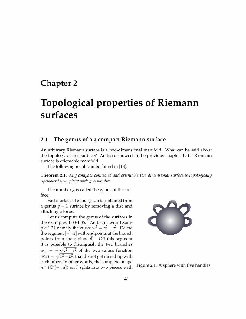
Theorem 2.1. Any compact connected and orientable two dimensional surface is topologicallyequivalent to a sphere with g ě handles.
Figure 2.1: A sphere with five handles
The number g is called the genus of the sur-face.
Each surface of genus g can be obtained froma genus g ´ 1 surface by removing a disc andattaching a torus.
Let us compute the genus of the surfaces inthe examples 1.33-1.35. We begin with Exam-ple 1.34 namely the curve w2 “ z2 ´ a2. Deletethe segment r´a, aswith endpoints at the branchpoints from the z-plane C. Off this segmentit is possible to distinguish the two branchesw˘ “ ˘
a
z2 ´ a2 of the two-values functionwpzq “
a
z2 ´ a2, that do not get mixed up witheach other. In other words, the complete imageπ´1pCzr´a, asq on Γ splits into two pieces, with
27

28 CHAPTER 2. TOPOLOGICAL PROPERTIES OF RIEMANN SURFACES
the mappingπ an isomorphism on each of them.The branches w`pzq and w´pzq are interchanged in passing from one edge of the cut r´a, asto the other. Therefore, the surface is glued together from two identical copies of sphereswith cuts according to the rule indicated in the figure 2.2
Figure 2.2: The cuts of the algebraic functiona
z2 ´ a2
After the gluing we again obtain a sphere, i.e., the genus g is equal to zero. Exam-ple 1.33 is analogous to Example 1.34, but the cut must be made between the points 0 and8, i.e. the point at infinity must be regarded as a branch point. Again the genus is equalto zero.
In Example 1.35 it is necessary to split up the branch points arbitrarily into pairs andmake cuts (arcs) in C joining the paired branch points n cuts for n even. The surface Γ isglued together from two identical copies of a sphere with such cuts, with the edges of thecorresponding cuts glued together in ”cross-wise” fashion (see the figure for n “ 4).
It is not hard to see that a sphere with n2 handles is obtained after the gluing, i.e., thegenus g is n2, see figure 2.4 for n “ 4. For n odd the situation is analogous, except thatin making the cuts it is necessary to take 8 as one of the branch points. The genus g isequal to pn` 1q2.
Exercise 2.2: Suppose that all the zeros z1 ă ¨ ¨ ¨ ă z2n`1 of the polynomial P2n`1pzq arereal. We choose the segments rz1, z2s, rz3, z4s, . . . , rz2n`1,8s of the real axis as the cuts forthe surface Γ “ tw2 “ P2n`1pzqu. The function wpzq “
a
P2n`1pzq which is single-valuedon each sheet of Γ formed after removal of the cycles π´1prz1, z2sq, . . . , π´1prz2n`1,8sq isreal on the edges of these cuts on each of the sheets. Show that on each sheet the sign ofthe square root
a
P2n`1pzq on the upper edge of the cut alternates.
2.1. THE GENUS OF A A COMPACT RIEMANN SURFACE 29
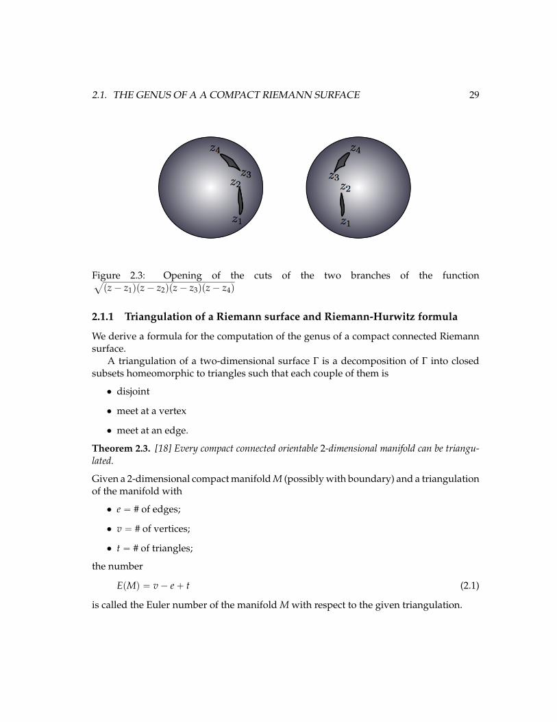
Figure 2.3: Opening of the cuts of the two branches of the functiona
pz´ z1qpz´ z2qpz´ z3qpz´ z4q
2.1.1 Triangulation of a Riemann surface and Riemann-Hurwitz formula
We derive a formula for the computation of the genus of a compact connected Riemannsurface.
A triangulation of a two-dimensional surface Γ is a decomposition of Γ into closedsubsets homeomorphic to triangles such that each couple of them is
• disjoint
• meet at a vertex
• meet at an edge.
Theorem 2.3. [18] Every compact connected orientable 2-dimensional manifold can be triangu-lated.
Given a 2-dimensional compact manifold M (possibly with boundary) and a triangulationof the manifold with
• e “ # of edges;
• v “ # of vertices;
• t “ # of triangles;
the number
EpMq “ v´ e` t (2.1)
is called the Euler number of the manifold M with respect to the given triangulation.
30 CHAPTER 2. TOPOLOGICAL PROPERTIES OF RIEMANN SURFACES
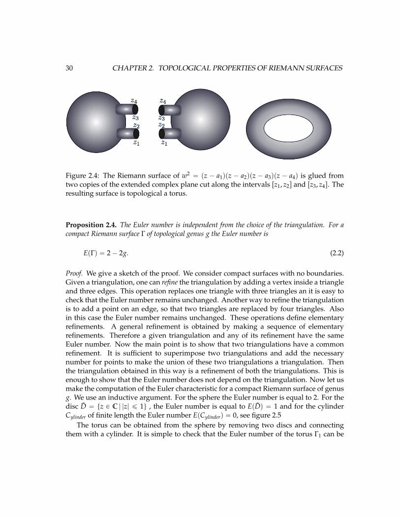
Figure 2.4: The Riemann surface of w2 “ pz ´ a1qpz ´ a2qpz ´ a3qpz ´ a4q is glued fromtwo copies of the extended complex plane cut along the intervals rz1, z2s and rz3, z4s. Theresulting surface is topological a torus.
Proposition 2.4. The Euler number is independent from the choice of the triangulation. For acompact Riemann surface Γ of topological genus g the Euler number is
EpΓq “ 2´ 2g. (2.2)
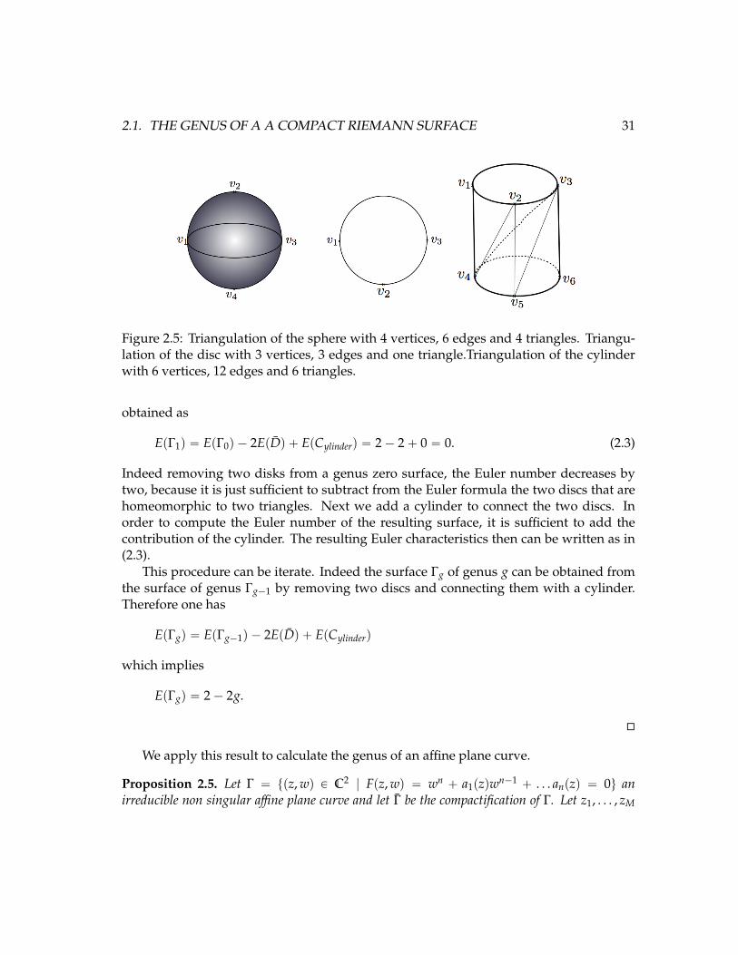
Proof. We give a sketch of the proof. We consider compact surfaces with no boundaries.Given a triangulation, one can refine the triangulation by adding a vertex inside a triangleand three edges. This operation replaces one triangle with three triangles an it is easy tocheck that the Euler number remains unchanged. Another way to refine the triangulationis to add a point on an edge, so that two triangles are replaced by four triangles. Alsoin this case the Euler number remains unchanged. These operations define elementaryrefinements. A general refinement is obtained by making a sequence of elementaryrefinements. Therefore a given triangulation and any of its refinement have the sameEuler number. Now the main point is to show that two triangulations have a commonrefinement. It is sufficient to superimpose two triangulations and add the necessarynumber for points to make the union of these two triangulations a triangulation. Thenthe triangulation obtained in this way is a refinement of both the triangulations. This isenough to show that the Euler number does not depend on the triangulation. Now let usmake the computation of the Euler characteristic for a compact Riemann surface of genusg. We use an inductive argument. For the sphere the Euler number is equal to 2. For thedisc D “ tz P C | |z| ď 1u , the Euler number is equal to EpDq “ 1 and for the cylinderCylinder of finite length the Euler number EpCylinderq “ 0, see figure 2.5
The torus can be obtained from the sphere by removing two discs and connectingthem with a cylinder. It is simple to check that the Euler number of the torus Γ1 can be
2.1. THE GENUS OF A A COMPACT RIEMANN SURFACE 31
Figure 2.5: Triangulation of the sphere with 4 vertices, 6 edges and 4 triangles. Triangu-lation of the disc with 3 vertices, 3 edges and one triangle.Triangulation of the cylinderwith 6 vertices, 12 edges and 6 triangles.
obtained as
EpΓ1q “ EpΓ0q ´ 2EpDq ` EpCylinderq “ 2´ 2` 0 “ 0. (2.3)
Indeed removing two disks from a genus zero surface, the Euler number decreases bytwo, because it is just sufficient to subtract from the Euler formula the two discs that arehomeomorphic to two triangles. Next we add a cylinder to connect the two discs. Inorder to compute the Euler number of the resulting surface, it is sufficient to add thecontribution of the cylinder. The resulting Euler characteristics then can be written as in(2.3).
This procedure can be iterate. Indeed the surface Γg of genus g can be obtained fromthe surface of genus Γg´1 by removing two discs and connecting them with a cylinder.Therefore one has
EpΓgq “ EpΓg´1q ´ 2EpDq ` EpCylinderq
which implies
EpΓgq “ 2´ 2g.
We apply this result to calculate the genus of an affine plane curve.
Proposition 2.5. Let Γ “ tpz,wq P C2 | Fpz,wq “ wn ` a1pzqwn´1 ` . . . anpzq “ 0u anirreducible non singular affine plane curve and let Γ be the compactification of Γ. Let z1, . . . , zM
32 CHAPTER 2. TOPOLOGICAL PROPERTIES OF RIEMANN SURFACES
be the branch point for Γ with respect to the projection πpz,wq Ñ z with multiplicity b1, . . . , bmrespectively. Then the genus of Γ is equal to
g “12
mÿ
j“1
b j ´ n` 1. (2.4)
Proof. Consider a triangulation of C so that the set of vertices of the triangulation containsthe points z1, . . . , zM. Suppose that for each triangle T in C, the projection π restricted tothe interior of each preimage π´1pTq is homeomorphic to the interior of T. In this waythe triangulation on C can be lifted to a triangulation on Γ. Suppose the triangulation ofC has v vertices, t triangles and e edges. Then the triangulation of Γ has
• t “ nt triangles
• e “ ne edges
• v “ nv´ b vertices,
where b “řm
j“1 b j. The Euler characteristic of the surface Γ gives
2´ 2g “ nv´ b´ ne` nt “ npv´ e` tq ´ b
so that one obtains the statement.
The relation (2.4) is a particular case of a more general formula known as Riemann-Hurwitz formula. As an application of the proposition 2.5 we calculate the genus of asmooth projective curve
Γ “ trX : Y : Zs P P2 |QpX,Y,Zq “ 0u
where Q is a homogeneous polynomial of degree n. Suppose that r0 : 0 : 1s < Γ so thatQp0, 0,Zq “ c Zn , 0 with c , 0. Then the map
φ : Γ Ñ P1, φpX,Y,Zq “ rX : Ys
realised Γ as a n-sheeted covering of P1. Let us calculate the total branching number ofthis map. The branch points are obtained by solving the equations
QpX,Y,Zq “ 0, QZpX,Y,Zq “ 0
The solution of the above two equations are given by the zeros of the resultant RpQ,QZq
with respect to Z. Since RpQ,QZq is a homogeneous polynomial of degree npn ´ 1q in Xand Y, the total number of branch points counting their multiplicity is npn´ 1q.
2.1. THE GENUS OF A A COMPACT RIEMANN SURFACE 33
Recall that the branching number of a branch point P0 “ rX0 : Y0 : Z0s indicated asbφpP0q is the order of the zero of QpX0,Y0,Zq at Z “ Z0 minus one. We can write
QpX0,Y0,Zq “ź
0ď jďs
pZ´ Z jqm j
whereř
j m j “ n and Z0, . . . ,Zs are distinct complex numbers, Z j “ Z jpX0,Z0q. Herewe assume that Qp0, 0,Zq “ Zn. With the above notation the branching number of eachbranch point P j “ rX0 : Y0 : Z js is bφpP jq “ m j ´ 1. So a regular point is simple zero ofQpX0,Y0,Zq a branch point with branching number one is a double zero, and a branchpoint with branching number m´ 1 is a zero of order m of QpX0,Y0,Zq. So if the numberof distinct roots of the discriminant is npn ´ 1q it means that the curve has npn ´ 1qbranch points with multiplicity one, so that the total branching number is npn ´ 1q. Ifthe discriminant has for example npn´ 1q ´ k distinct roots, k ą 0, it means that some ofthe branch points have branching number bigger then one. However the total branchingnumber remains equal to npn´ 1q. Then we can apply formula 2.4 to obtain
g “12pn´ 1qn´ n` 1
which gives g “12pn´ 2qpn´ 1q.
Lemma 2.6. The genus of a smooth projective curve of degree n is given by the relation
g “12pn´ 2qpn´ 1q. (2.5)
Exercise 2.7: Calculate the genus of the following surfaces
w3 “ pz´ 1qpz´ 2qpz´ 3qpz´ 4q,
wn “ zn ` an, a , 0.
Theorem 2.8. [14] Any compact connected orientable two-dimensional surface of genus g thatadmits a triangulation, can be made into a Riemann surface.
Any surface of genus zero is topologically equivalent to the sphere P1. The surfacesof genus one are one-dimensional tori. The complex structure is unique only for g “ 0(see [14] 16.13). The set of complex structures has one complex parameter for g “ 1 and3g´ 3 complex parameters for g ě 2. The space of these parameters is called Teichmullerspace. We observe that the number 3g ´ 3 coincides with the dimension of the modulispace of Riemann surfaces of genus g ě 2.
34 CHAPTER 2. TOPOLOGICAL PROPERTIES OF RIEMANN SURFACES
2.2 Monodromy of a surface
In order to define the monodromy of a surface we recall the definition of fundamentalgroup. Let M be a topological space and P, Q two points on M. A curve u : I Ñ Mstarting in P and ending in Q is a continuous map from Ir0, 1s to M such up0q “ P andup1q “ Q. If two curves can be deformed continuously one into the other, the curves arecalled homotopic.
Definition 2.9. Two curves u and w are homotopic if there is a continuos map A : I ˆ I Ñ Msuch
• Apt, 0q “ uptq,
• Apt, 1q “ wptq,
• Ap0, sq “ P and Ap1, sq “ Q, for all s P r0, 1s.
The notion of homotopic is an equivalence relation. It is easy to construct homotopiccurves. For example given a smooth map f : I Ñ I, the curves u and u ˝ f are homotopic.In the space of curves we can define a group structure.
Definition 2.10. Given two curves u : I Ñ M and w : I Ñ M, I “ r0, 1s, such that up0q “ Pand up1q “ Q and wp0q “ Q and wp1q “ R the product curve is
pu ˝ wqptq :“"
up2tq for 0 ď t ď 12
wp2t´ 1q for 12 ď t ď 1 ,
the inverse of a curve is
u´1ptq :“ up1´ tq, t P I,
the constant curve is
Id : I Ñ M, Idptq “ P.
Clearly u ˝ u´1 is homotopic to Id. Now let us consider curves starting and ending inP, namely close loops.
Definition 2.11. Let M be a topological space. The set of homotopic classes of loops starting andending in P P M is denoted by π1pM,Pq.
The set π1pM,Pq forms a group under the operation induced by the product of curves.We denote its elements by rγs. It is easy to check that for arc-wise connected spaces M,the group π1pM,Pq is independent from the base point P. Indeed let π1pM,Qq be thefundamental group with base point Q, and let w be a path from P to Q. Then for anyelement rγs P π1pM,Pq the loop rw´1 ˝ γ ˝ws P π1pM,Qq and this map is an isomorphism.
2.2. MONODROMY OF A SURFACE 35
Definition 2.12. An arc-wise topological space M is called simply connected if π1pMq “ 0.
Remark 2.13. We remind that the only Riemann surfaces with trivial fundamental groupare the sphere the complex plane and the disk. The only Riemann surface M withπ1pMq “ Z is the punctured disk or the punctured complex plane. The only compactRiemann surface M with π1pMq “ ZˆZ is the torus.
Although the trivial element of the group is the identity, it has become standardnotation to write π1pMq “ 0 for the fundamental group that contains only the identity. Ina simply connected space all loops are homotopic to the identity loop. The sphere P1 is asimply connected space.
Now we are ready to define the monodromy group of a surface. Consider a compactRiemann surface Γ realised as the compactification of a smooth affine plane curve
Γ “ tpz,wq P C2|Fpz,wq “ z2 ` a1pzqwn´1 ` ¨ ¨ ¨ ` anpzq “ 0u
and consider the projection π : Γ Ñ C, πpz,wq “ z and denote by z1, . . . , zM the branchpoint of such map. Let delete from C the branch points z1, . . . , zM and delete from Γthe complete inverse images π´1pz1q, . . . , π´1pzMq of these points. We get a surface Γ0that is a n-sheeted covering of the punctured sphere Czpz1 Y ¨ ¨ ¨ Y zMq. The monodromygroup of the Riemann surface is the monodromy group of this covering. We recall thegeneral definition of the monodromy group of a covering in connection with this case(see [9] for more details). Fix a point z0 P Czpz1 Y ¨ ¨ ¨ Y zMq and number the pointsP1, . . . ,Pn in the fiber π´1pz0q arbitrarily (these points are all distinct). Any closed contourin Czpz1 Y ¨ ¨ ¨ Y zMq beginning and ending at z0 gives rise to a permutation of the pointsP1, . . . ,Pn of the fiber after being lifted to Γ0. We get a representation of the fundamentalgroup π1pCzpz1Y¨ ¨ ¨YzMq, z0q in the group Sn of permutations of n elements; this is calledthe monodromy representation. Let γk, k “ 1, . . . ,M be a loop starting and ending in z0and encircling the point zk, k “ 1, . . . ,M. We denote by rγks the homotopy class of thisloop. The loops rγ1s, . . . , rγMs are generators ofπ1pCzpz1Y¨ ¨ ¨YzMq, z0qwith the constraint
rγ1s ˝ rγ2s ˝ ¨ ¨ ¨ ˝ rγns “ Id (2.6)
namely the trivial loop. The mondromy representation
ρ : π1pCzpz1 Y ¨ ¨ ¨ Y zMq, z0q Ñ Sn, ρprγksq “ σk
is a group homomorphism namely
ρprγks ˝ rγ jsq “ σkσ j, (2.7)
for any set of generators. The homotopy relation (2.6) implies
σ1σ2 . . . σM “ Id
the identity in Sn.
36 CHAPTER 2. TOPOLOGICAL PROPERTIES OF RIEMANN SURFACES
Definition 2.14. The image of the map ρ defined in (2.7) in Sn is called the monodromy group ofthe surface Γ.
Remark 2.15. For connected surfaces, the image of the monodromy group is a transitivesubgroup in Sn. Indeed a transitive subgroup G P Sn has the property that for everynumber i, j P t1, . . . ,nu there exists a permutation τ P G such that j “ τpiq. If the Riemannsurface is connected, for any points Pi and P j in the fiber π´1pzq, z P C it is possible to finda path connecting these points.
For hyperelliptic Riemann surfaces the monodromy group coincides S2 “ Z2.
Exercise 2.16: For curves of the form
wn “
Nź
j“1
pz´ ziq
show that the monodromy group coincides with Zn.
In the general case the action of the generators of the monodromy group that corre-spond to circuits about branch points is determined by the branching indices.
Exercise 2.17: Let z be a branch point, and let the complete inverse image π´1pzq on Γconsist of the ramification points P1, . . . ,Pk of multiplicity b1, ..., bk, respectively (if somepoint Pi is not a branch point, then we set bi “ 0). Prove that to a cycle in C encircling z0once there corresponds an element in the monodromy group splitting into cycles of lengthb1 ` 1, ..., bk ` 1. This assertion gives a purely topological definition of the multiplicities(indices) of branch points.
Remark 2.18. Suppose that one of the branch points, let say zM “ 8. Then the mon-odromy corresponding to circuits about the point z “ 8 is uniquely determined by themonodromy corresponding to circuits about the images of the finite branch points. In-deed, a contour encircling only the point z “ 8 splits into a product of contours encirclingall the finite branch points, and we get the monodromy at infinity by multiplying the cor-responding elements of the monodromy groups at the finite points. For example, for thesurface w2 “ P2n`2pzq the monodromy at infinity is trivial (the corresponding contour inthe z-plane encircles an even number of branch points), i.e., this surface has no branchpoints at infinity. But for the surface w2 “ P2n`1pzq the monodromy at infinity is nontriv-ial, because here a contour encircling z “ 8 encircles an odd number of branch points.We thus see once more that the point at infinity of the surface w2 “ P2n`1pzq is a branchpoint.
Exercise 2.19: Prove that for a general surface of the form (1.26)) the monodromy groupcoincides with the complete symmetric group Sn . Hint. Show that the branch points of such
2.3. SINGULAR CURVES 37
a surface can be labeled by pairs of distinct numbers i , j, pi, j “ 1, ...,nq in such a way that acircuit about the images of the points Pi j and P ji gives rise to a transposition of the ith and jthpoints of the fiber ( when these points are suitably numbered).
2.3 Singular curves
Let us consider an affine plane curve
Γ “ tpz,wq P C2|Fpz,wq “ z2 ` a1pzqwn´1 ` ¨ ¨ ¨ ` anpzq “ 0u.
A point P0 “ pz0,w0q P Γ is called singular if
Fpz0,w0q “ Fzpz0,w0q “ Fwpz0,w0q “ 0.
If the polynomial F is irreducible then the set of singular points is finite.
Nodes of an affine plane curve. The singular point P0 “ pz0,w0q P Γ is called a nodeif the Hessian
detˆ
Fzzpz0,w0q Fzwpz0,w0q
Fzwpz0,w0q Fwwpz0,w0q
˙
, 0.
We can expand in Taylor series the equation of the curve near the node P0 “ pz0,w0q toobtain
Fpz,wq “ α1pz´ z0q2 ` α2pz´ z0qpw´ w0q ` α3pw´ w0q
2 ` higher order tems
where α1 “ Fzzpz0,w0q2, α2 “ Fzwpz0,w0q and α3 “ Fwwpz0,w0q. The quadratic term is ahomogenous polynomial that can be factor in the product of two first order homogeneouspolynomials namely
Fpz,wq “ pc1pz´ z0q ` c2pw´ w0qqpb1pz´ z0q ` b2pw´ w0qq ` higher order tems,
Defining x “ c1pz´ z0q ` c2pw´ w0q and y “ b1pz´ z0q ` b2pw´ w0q one has
Fpz,wq “ xy`ÿ
jě2
f jpx, yq
where f j are homogenous polynomials of degree j in x and y. Applying Hensel’s Lemma,which say that if the lower order term of a power series factor, then the entire powerseries can factor compatibly, we can write the above expansion in the form
Fpz,wq “ rpx, yqspx, yq
38 CHAPTER 2. TOPOLOGICAL PROPERTIES OF RIEMANN SURFACES
with
rpx, yq “ x`ÿ
jě2
r jpx, yq, spx, yq “ y`ÿ
jě2
s jpx, yq
where each r jpx, yq and s jpx, yq is a homogeneous polynomial of degree j that can beobtained uniquely from the polynomials fk. Since Fpz,wq is a polynomial the power seriesfor the function rpx, yq and spx, yq are clearly convergent.
Near the node pz0,w0q the curve is the locus of zeros of rpx, yqspx, yqwhich is the unionof the locus of zeros of the functions rpx, yq and the locus of zeros of spx, yq. Each locuscorresponds to a curve Γr and Γs respectively. These curves are nonsingular in P0. Now wecall Γ the curve obtained from the singular curve Γ by removing the point P0. The curveΓ looks locally as the union ΓrztP0u and ΓsztP0u. Let us consider open sets Ur and Us on Γwhich are equal to open set on ΓrztP0u and ΓsztP0u. Such open sets are homeomorphic topuncture disks. According to definition 1.36, the surface Γ is a Riemann surface with twopunctures. Compactifying the curve Γ according to section 1.1.3, one obtains a smoothcompact Riemann surface S. The whole process is called resolving the nodes of Γ. Thesmooth compact Riemann surface obtained in this way is called also the normalisation ofΓ.
Genus of a projective curve with nodes. Let us consider a projective curve with knodes defined by the zeros FpX,Y,Zq “ 0 of the homogeneous polynomial F of degree n.In order to compute the genus of the smooth curve Γ,obtained from Γ by resolving thenodes, it is necessary to observe that for each node the total branching number of the curvedecreases by two, indeed perturbing slightly the polynomial equation near the node, twobranch points with multiplicity one are obtained. Then using Riemann-Hurwitz formula(2.4) one obtains the genus of a projective curve with nodes, namely Plucker’s formula.
Proposition 2.20. Let Γ be a projective curve of degree n with k nodes and no other singularities.Then the genus of Γ the curve obtained by resolving the nodes of Γ is
g “12pn´ 1qpn´ 2q ´ k.
Monomial singularities
A curve Γ defined by the zero of the polynomial Fpz,wq “ 0 has a singular point in p0, 0qcalled a monomial singularity if locally the polynomial Fpz,wq is of the form
Fpz,wq “ wn ´ zm,
with m and n integers. If m “ n “ 2 the singular point is a node, and for n “ 2 and m “ 2kit is a higher order node. In the case n “ 2 and m “ 3 the singularity is a cusp and for
2.3. SINGULAR CURVES 39
m “ 2k ` 1 it is called a higher order cusp. In general when n and m are co-prime thesingularity is called a monomial singularity of type pm,nq. If mn “ kpkq with k, p and qintegers and p and q relatively prime, then the monomial singularity can be factored as
Fpz,wq “kź
j“1
pwq ´ ξ jzpq, ξ “ e2πik .
Let us consider a monomial singularity with pm,nq co-prime. Then near such singularitythe curve has a parametrisation t Ñ ptn, tmq. Let us consider the puncture neighbourhoodof p0, 0q in Γ, namely the set
U “ tpz,wq P C2 : 0 ă |z| ă ρ, and Fpz,wq “ 0u
and the disc
D “ tt P C : |t| ă ρ1n u.
The map
Ψ : Dzt0u Ñ U, Φptq “ ptn, tmq
is a biholomorphic map from Dzt0u to U. The inverse map is given by
Φpz,wq Ñ zawb “ t, an`mb “ 1
with a and b integers. The map Φ is compatible with the complex structure of Γ. So thecurve Γztp0, 0u is a Riemann surface with punctures according to definition 1.36. We canextend the map Φ : U Y tp0, 0qu Ñ D by defining Φp0, 0q “ 0. The Riemann surface thatwe obtain is a smooth compact Riemann surface S.
Resolution of singularities of general curves and Puiseux expansion
Resolution of singularities of curves was essentially first proved by Newton (1676), whoshowed the existence of Puiseux series for a curve from which the resolution of singulari-ties follows easily. Puiseux series are a generalisation of powers series and they were firstintroduced by Newton and then they were rediscovered by Puiseux in 1850. A Puiseuxseries in the variable z is a power series of the form
ř8j“k a jz jn where k is an integer and
n is a positive integer.Let us consider the polynomial equation Fpz,wq “ 0. When
gradF “ pFzpz0,w0q,Fwpz0,w0qq , p0, 0q

40 CHAPTER 2. TOPOLOGICAL PROPERTIES OF RIEMANN SURFACES
the implicit function theorem gives a local parametrisation of the curve
z Ñ pz, ψpzqq
in the case Fwpz0,w0q , 0, and ψpzq is an analytic function of z in the neighbourhood ofz “ z0. Therefore the curve looks locally like the graph of a function which is locally likeits tangent line. For singular curves such parametrisation does not exist, like for examplefor the curve Fpz,wq “ w2 ´ z3. However there is a parametrisation of the form
t Ñ pt2, t3q, or z Ñ pz, z32 q.
Locally any singular branch of a curve has a parametrisation of the form
t Ñ ptn, ψptqq, or pz, ψpz1n qq, k ą 1,
for some power series ψ. Such series is called Puiseux series. The next theorem, calledPuiseux’s theorem, asserts that, given a polynomial equation Fpz,wq “ 0, its solutions inw, viewed as functions of z, may be expanded as convergent Puiseux series. Suppose thethe point pz0,w0q is a singular point of the curve defined by Fpz,wq “ 0. Furthermorewe assume for simplicity that the pre-image of the point z0 with respect to the projectionπpz,wq Ñ z consists only of one point, namely π´1pz0q “ w0.
Theorem 2.21. Let Fpz,wq be a polynomial such that Fp0,wq , 0 and deg Fp0,wq “ n. Foreach point near z0, there are homolorphic functions ψ1ptq, . . . , ψlptq defined near t “ 0, such thatψ jp0q “ w0 and positive integers m1, . . . ,ml with m1 ` ¨ ¨ ¨ `ml “ n such that
Fpz0 ` tm j , ψ jptqq “ 0, j “ 1, . . . , l.
In other words for every z sufficiently close to z0 the polynomial Fpz,wq can be factored in the form
Fpz,wq “ cl
ź
j“1
m jź
s“1
ˆ
w´ ψ jpe2πism jpz´ z0q1
mj q
˙
.
Two Puiseux expansions with indices j , j are essentially different. Newton gavean algorithm to construct such parametrisations that it is know as Newton polygontechnique. We are not going to enter the details of this technique. We give only someexamples.Example 2.22. Suppose that Fpz,wq is a polynomials with deg Fp0,wq “ k, such that thereare integers numbers p and q such that
Fpz,wq “ÿ
qi`pj“kp
ai jziw j.
2.3. SINGULAR CURVES 41
Then we can look for a parametrisation of the form Fptq, λtpq “ 0, namely
Fpz,wq “ Fptq, λtpq “ tkpÿ
iq`pj“kp
ai jλj :“ tkphpλq
We can always find λ0 P C such that hpλ0q “ 0.In general for a polynomial
Fpz,wq “ÿ
i j
ai jziw j
the carrier C of F is defined as
CpFq “ tpi, jq P Z2 | ai j , 0u.
The Newton polygon is the convex hull of the points in the carrier. We can assumewithout loss of generality that the Newton polygon touches both axis. Suppose that thereare rational number µ and ν such that
Fpz,wq “ÿ
i`µ jěν
ai jziw j.
Then the the line
z` µw “ ν
lies below the carrier CpFq. Now substituting w “ tzµ into F we get
Fpz, tzµq “ zνÿ
i`µ j“ν
ai jt j `ÿ
i`µ jąν
ai jzi`µ j “ zνÿ
i`µ j“ν
ai jt j ` opzνq.
Let t0 be a solution of the equationř
i`µ j“ν ai jt j “ 0. Note that this equation has a solutionif there are at least two points of the carrier CpFq on the line z ` µw “ ν. Then we canconsider pz, t0zµq as an approximate solution of the equation Fpz,wq “ 0 near the singular
point p0, 0q. The next step is to improve the above approximation. Assuming µ “pq
with
p and q integers that do not have a common factor, one can look for an expansion of theform
z1 “ zq, w “ zp1pt0 ` w1q.
Then plugging the above ansatz into Fpz,wq one obtains
Fpzq1, z
t1pt0 ` w1qq “ zqν
1 F1pz1,w1q.
The next step is to study the singularity structure of the polynomial F1pz1,w1q. By iteratingthis procedure, one obtains the Puiseux expansion near the point p0, 0q.
42 CHAPTER 2. TOPOLOGICAL PROPERTIES OF RIEMANN SURFACES
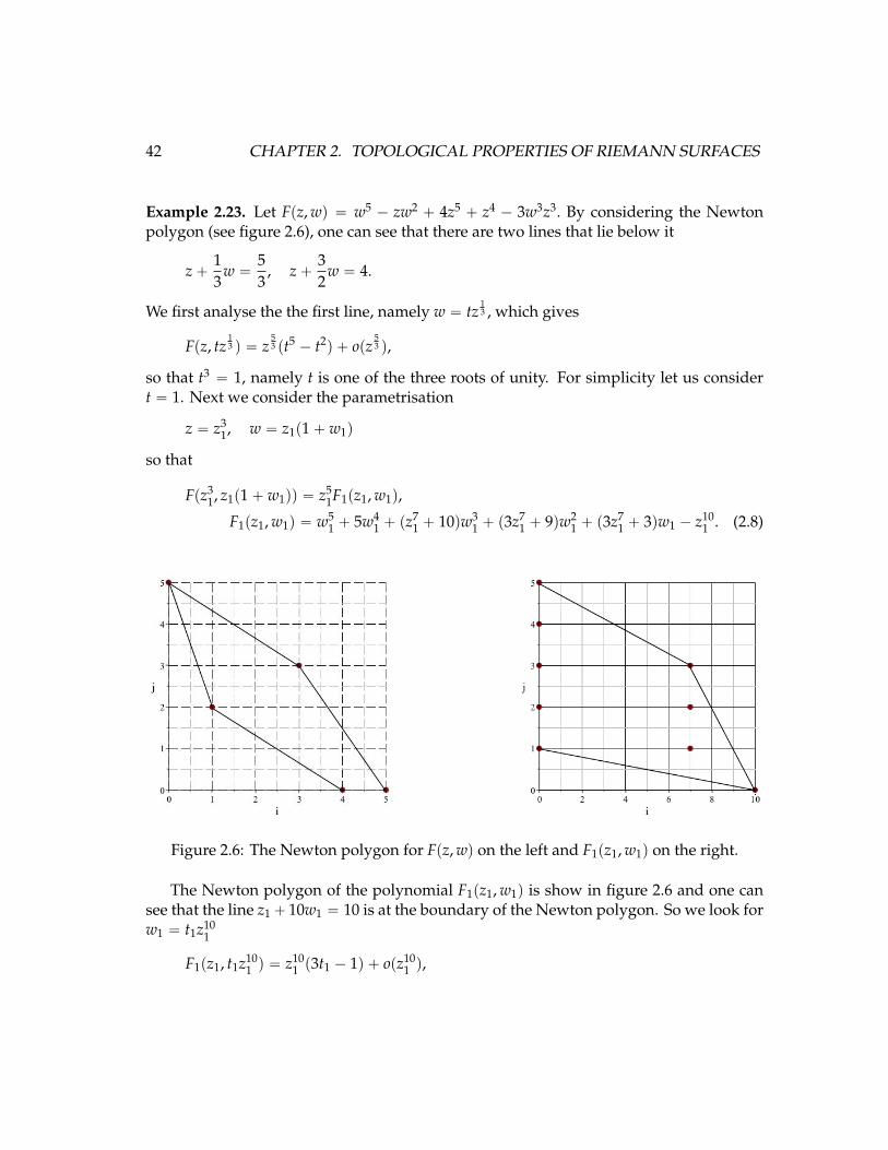
Example 2.23. Let Fpz,wq “ w5 ´ zw2 ` 4z5 ` z4 ´ 3w3z3. By considering the Newtonpolygon (see figure 2.6), one can see that there are two lines that lie below it
z`13
w “53, z`
32
w “ 4.
We first analyse the the first line, namely w “ tz13 , which gives
Fpz, tz13 q “ z
53 pt5 ´ t2q ` opz
53 q,
so that t3 “ 1, namely t is one of the three roots of unity. For simplicity let us considert “ 1. Next we consider the parametrisation
z “ z31, w “ z1p1` w1q
so that
Fpz31, z1p1` w1qq “ z5
1F1pz1,w1q,
F1pz1,w1q “ w51 ` 5w4
1 ` pz71 ` 10qw3
1 ` p3z71 ` 9qw2
1 ` p3z71 ` 3qw1 ´ z10
1 . (2.8)
Figure 2.6: The Newton polygon for Fpz,wq on the left and F1pz1,w1q on the right.
The Newton polygon of the polynomial F1pz1,w1q is show in figure 2.6 and one cansee that the line z1` 10w1 “ 10 is at the boundary of the Newton polygon. So we look forw1 “ t1z10
1
F1pz1, t1z101 q “ z10
1 p3t1 ´ 1q ` opz101 q,
2.3. SINGULAR CURVES 43
which gives t1 “13 . We conclude that the first two terms of the Puiseux expansion are
w “ z13 `
13
z113 ` . . . .
Repeating the same procedure for the coefficient µ “32
one obtains
w “ p´zq32 ´
12p´zq
52 ` . . . .
Summarizing we have obtained two essentially different Puiseux expansions near thepoint p0, 0q.
Once the Puiseux series for a curve near a singular point has been found the resolutionof the singularity follows easily.
Theorem 2.24. For every irreducible algebraic curve Γ P P2 there exists a compact Riemannsurface S and a holomorphic map
φ : S Ñ Γ
with the properties
• let Γ :“ ΓzSing Γ be the smooth part of Γ and let S :“ φ´1pΓq. Then
φ :“ φ|S : S Ñ Γ
is bi-holomorphic
• φ : S Ñ Γ is surjective.
For a singular point P P Sing Γ, the number of points in the preimage of φ´1pPq isgiven the by the number of essentially different Puiseux expansions of Γ near P. In theexample 2.23 the number of pre-images of the singular point p0, 0q consists of two points.
Exercise 2.25: Calculate the genus of the singular curves
w3 “ pz´ a1q2pz´ a2qpz´ a3q
2pz´ a4q
and
w3 “ z3pz´ a3q2pz´ a4q.
For each singular point calculate the number of points in the preimage of the map φdefined in theorem 2.24.
44 CHAPTER 2. TOPOLOGICAL PROPERTIES OF RIEMANN SURFACES
Exercise 2.26: For which value of λ the following curves are non singular?
X3 ` Y3 ` Z3 ` 3λXYZ “ 0
and
X3 ` Y3 ` Z3 ` λpX ` Y` Zq3 “ 0.
Describe the singularities when they exist and calculate the genus of the correspondingRiemann surface.
2.4 Homology
In this section we define the homology of a Riemann surface.Given a triangulation of a Rieamnn surface we define the vertex as 0-simplex, the edges
as 1-simplex and the triangles as 2-simplex. The orientation on the manifold induces anorientation on the triangles that can be used to orient the edges bounding each triangle.
Definition 2.27. Given a triangulation of a Riemann surface, a simplicial 0, 1 and 2 chain is aformal sum of vertices, P j, edges e j or triangles t j
c0 “ÿ
j
n jP j, c1 “ÿ
j
m je j, c2 “ÿ
j
k jt j.
The set of n-chain Cn has a natural structure of additive abelian group.
The element ´c1 is the edge with opposite orientation and ´t is the triangle with op-posite orientation. The vertices P1, P2, P3, . . . can be used to identify edges and triangles.For example xP1P2y is the oriented edge from P1 to P2 and xP1,P2,P3y is the orientedtriangle with sides the oriented edges xP1P2y, xP2P3y and xP3P1y. With this notation wedefine the boundary operator δ
Definition 2.28. The boundary operator δ : Cn Ñ Cn´1 with n “ 0, 1, 2 is defined as follows:
δc0 “ 0, c0 P C0
δxP1P2y “ P2 ´ P1
δxP1,P2,P3y “ xP1P2y ` xP2P3y ` xP3P1y.
The above relation defines δ on 1 and 2-simplex and it can be extend to 1 and 2-chain by linearity.
2.4. HOMOLOGY 45
With the above definition it is immediate to observe that δ2 “ 0. Furthermore, δ is agroup homomorphism from Cn to Cn´1. We define
Zn “ tcn P Cn | δcn “ 0u, Bn “ tcn P Cn | Dcn`1 P Cn`1, cn “ δcn`1u.
From the above definition it is clear that
Bn Ď Zn Ď Cn
Since all the groups are abelian, Bn is a normal subgroup. We are interested in thefollowing quotient groups.
Definition 2.29. The n-homology group of Γ is defined as
HnpΓ,Zq “Zn
Bn, n “ 0, 1, 2.
We remark that the homology groups are independent from the triangulation. A basisfor HnpΓ,Zq is the set of elements of HnpΓ,Zq such that any other element can be writtenas a linear integer combination of elements of the basis. It is clear from the definitionthat dimH0pΓ,Zq “ 1. Regarding H2pΓ,Zq, with a little thought it is easy to see that fora compact Riemann surface dimH2pΓ,Zq “ 1. The only nontrivial group is H1pΓ,Zq. Wehave the following result.
Theorem 2.30. The first homology group H1pΓ,Zq is isomorphic to the abelianization of the firsthomotopy group πpΓq. The group H1pΓ,Zq is a free abelian group with 2g generators. Any cyclecan be written as a sum of of generators.
The theorem above gives the following. Let Γ be a compact Riemann surface of genusg and let rγ1s, . . . , rγ2gs be the set of generators of π1pΓq. Then any element rγs P π1pΓq canbe uniquely written as
rγsπ1 “ rγk1sj1π1˝ rγk2s
j2π1˝ . . . rγkns
jnπ1, k1, . . . kn P t1, 2, . . . , 2gu
with j1, . . . , jn P Z and where we put an under script of π1 to denote an element of thefundamental group. Then the corresponding element rγsH1 in the homology is obtainedas
rγsH1 “ j1rγk1sH1 ` j2rγk2sH1 ` ¨ ¨ ¨ ` jnrγknsH1 , k1, . . . kn P t1, 2, . . . , 2gu.
In the rest of this section we simply denote as γ an element in the homology basis.Let a1, . . . , ag, b1, . . . , bg be a basis in H1pΓ,Zq. Then any cycle γ is homologous to a linearcombination of the basis with integer coefficients:
γ »gÿ
i“1
miai `
gÿ
i“1
nibi, mi, ni P Z.
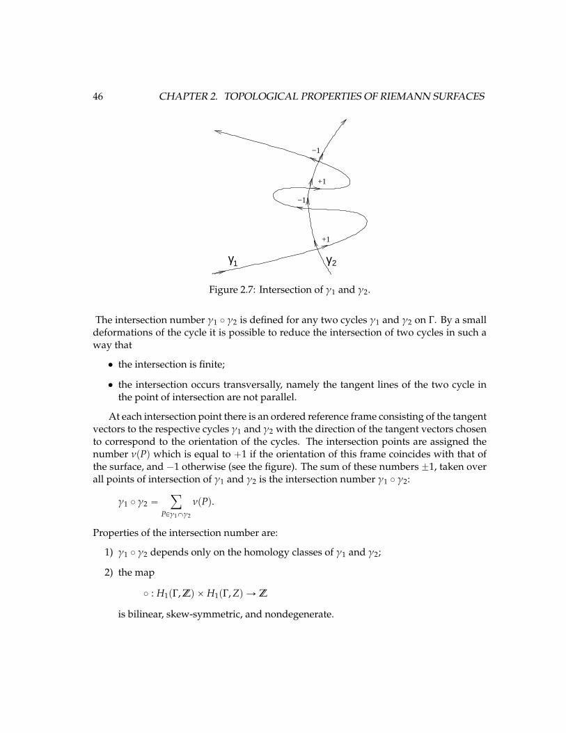
46 CHAPTER 2. TOPOLOGICAL PROPERTIES OF RIEMANN SURFACES
+1
−1
+1
−1
γ1 γ2
Figure 2.7: Intersection of γ1 and γ2.
The intersection number γ1 ˝ γ2 is defined for any two cycles γ1 and γ2 on Γ. By a smalldeformations of the cycle it is possible to reduce the intersection of two cycles in such away that
• the intersection is finite;
• the intersection occurs transversally, namely the tangent lines of the two cycle inthe point of intersection are not parallel.
At each intersection point there is an ordered reference frame consisting of the tangentvectors to the respective cycles γ1 and γ2 with the direction of the tangent vectors chosento correspond to the orientation of the cycles. The intersection points are assigned thenumber νpPq which is equal to `1 if the orientation of this frame coincides with that ofthe surface, and ´1 otherwise (see the figure). The sum of these numbers ˘1, taken overall points of intersection of γ1 and γ2 is the intersection number γ1 ˝ γ2:
γ1 ˝ γ2 “ÿ
PPγ1Xγ2
νpPq.
Properties of the intersection number are:
1) γ1 ˝ γ2 depends only on the homology classes of γ1 and γ2;
2) the map
˝ : H1pΓ,Zq ˆH1pΓ,Zq Ñ Z
is bilinear, skew-symmetric, and nondegenerate.
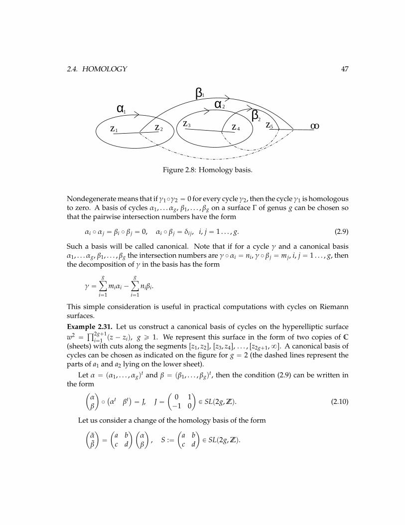
2.4. HOMOLOGY 47
oozz zz z
βα
βα5
1 23
4
1
1
2
2
Figure 2.8: Homology basis.
Nondegenerate means that if γ1˝γ2 “ 0 for every cycle γ2, then the cycle γ1 is homologousto zero. A basis of cycles α1, . . . αg, β1, . . . , βg on a surface Γ of genus g can be chosen sothat the pairwise intersection numbers have the form
αi ˝ α j “ βi ˝ β j “ 0, αi ˝ β j “ δi j, i, j “ 1 . . . , g. (2.9)
Such a basis will be called canonical. Note that if for a cycle γ and a canonical basisα1, . . . αg, β1, . . . , βg the intersection numbers are γ ˝αi “ ni, γ ˝ β j “ m j, i, j “ 1 . . . , g, thenthe decomposition of γ in the basis has the form
γ “gÿ
i“1
miαi ´
gÿ
i“1
niβi.
This simple consideration is useful in practical computations with cycles on Riemannsurfaces.Example 2.31. Let us construct a canonical basis of cycles on the hyperelliptic surfacew2 “
ś2g`1i“1 pz ´ ziq, g ě 1. We represent this surface in the form of two copies of C
(sheets) with cuts along the segments rz1, z2s, rz3, z4s, . . . , rz2g`1,8s. A canonical basis ofcycles can be chosen as indicated on the figure for g “ 2 (the dashed lines represent theparts of a1 and a2 lying on the lower sheet).
Let α “ pα1, . . . , αgqt and β “ pβ1, . . . , βgq
t, then the condition (2.9) can be written inthe form
ˆ
αβ
˙
˝`
αt βt˘
“ J, J “ˆ
0 1´1 0
˙
P SLp2g,Zq. (2.10)
Let us consider a change of the homology basis of the formˆ
αβ
˙
“
ˆ
a bc d
˙ˆ
αβ
˙
, S :“ˆ
a bc d
˙
P SLp2g,Zq.
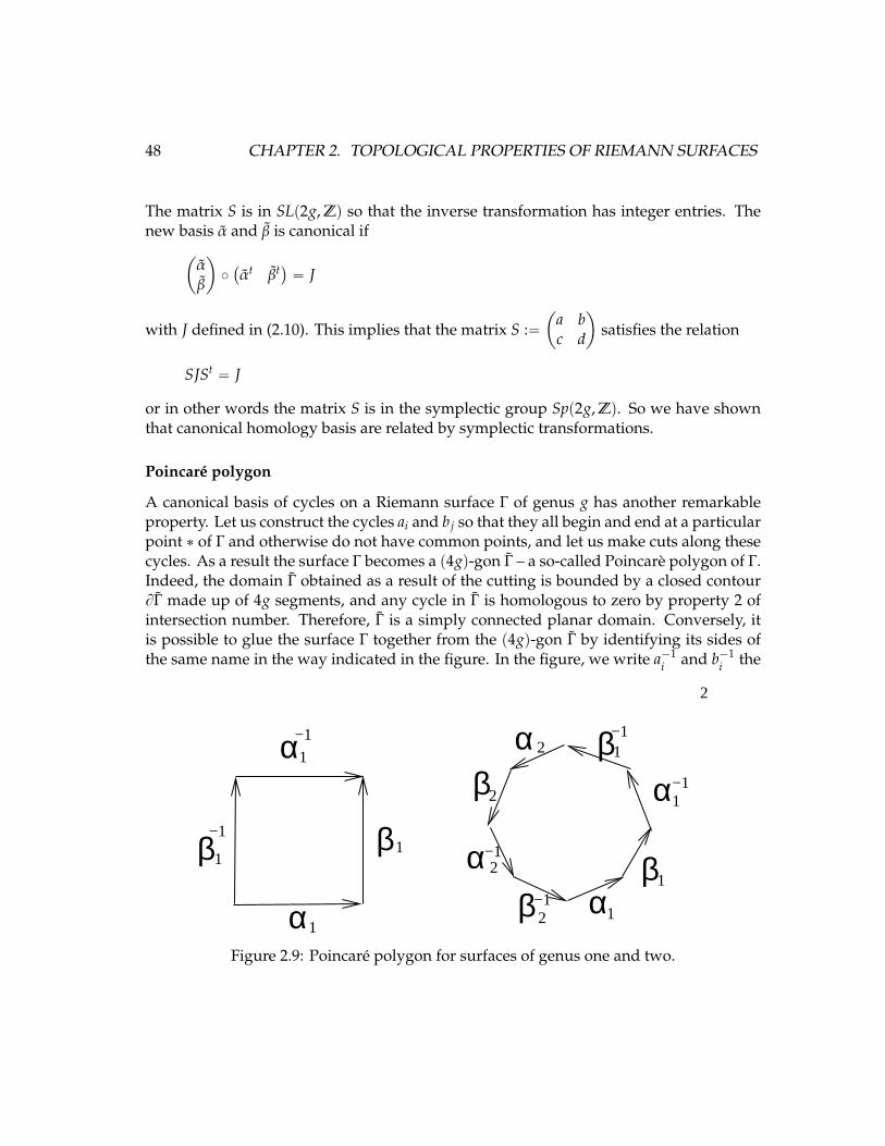
48 CHAPTER 2. TOPOLOGICAL PROPERTIES OF RIEMANN SURFACES
The matrix S is in SLp2g,Zq so that the inverse transformation has integer entries. Thenew basis α and β is canonical if
ˆ
αβ
˙
˝`
αt βt˘
“ J
with J defined in (2.10). This implies that the matrix S :“ˆ
a bc d
˙
satisfies the relation
SJSt “ J
or in other words the matrix S is in the symplectic group Spp2g,Zq. So we have shownthat canonical homology basis are related by symplectic transformations.
Poincare polygon
A canonical basis of cycles on a Riemann surface Γ of genus g has another remarkableproperty. Let us construct the cycles ai and b j so that they all begin and end at a particularpoint ˚ of Γ and otherwise do not have common points, and let us make cuts along thesecycles. As a result the surface Γ becomes a p4gq-gon Γ – a so-called Poincare polygon of Γ.Indeed, the domain Γ obtained as a result of the cutting is bounded by a closed contourBΓ made up of 4g segments, and any cycle in Γ is homologous to zero by property 2 ofintersection number. Therefore, Γ is a simply connected planar domain. Conversely, itis possible to glue the surface Γ together from the p4gq-gon Γ by identifying its sides ofthe same name in the way indicated in the figure. In the figure, we write a´1
i and b´1i the
α
β
α
1
−1
1β−1
β
β
1
1
1
1
2
2
−12
2−1
1
1
α
α
αβ
β2−1
−1α
Figure 2.9: Poincare polygon for surfaces of genus one and two.
2.4. HOMOLOGY 49
edges of the cut along the cycles ai and bi, respectively, if these edges occur in the orientedboundary BΓ with a minus sign. The segment ai is glued together with the segment a´1
iand bi with the segment b´1
i in the direction indicated by the arrows.
50 CHAPTER 2. TOPOLOGICAL PROPERTIES OF RIEMANN SURFACES
Chapter 3
Meromorphic functions on aRiemann surface.
3.1 Holomorphic mappings of Riemann surfaces
Definition 3.1. Let Γ be a Riemann surface. A function f : Γ Ñ C is said to be holomorphic, iffor each local chart the function
f ˝ φ´1α : φαpUαq Ñ Vα Ă C
zα Ñ fαpzαq :“ f pφ´1α pzαqq,
is holomorphic on the open subset φαpUαq.
The following theorem is inherited from complex analysis.
Theorem 3.2. If Γ is a connected compact Riemann surface, then the only holomorphic functionsare constants.
Proof. Since f is holomorphic, | f | is continuos on Γ compact. Therefore | f | achieves itsmaximum value at some point of Γ. By the maximum modulus Theorem, f must beconstant on Γ since Γ is connected.
In the same way one can define meromorphic functions.
Definition 3.3. A function f is a meromorphic function on a Riemann surface Γ if it is holomorphicin a neighborhood of any point of Γ except for finitely many points Q1, . . . ,Qm. At the pointsQ1, . . . ,Qm the function f has poles of respective multiplicities q1, . . . , qm i.e., in a neighborhoodof the point Q j, j “ 1, . . . ,m, it can be represented in the form
f “ τ´qij f jpτ jq, (3.1)
51
52 CHAPTER 3. MEROMORPHIC FUNCTIONS ON A RIEMANN SURFACE.
where τ j is a local parameter centred at the point Q j, and f jpτ jq is a holomorphic function for smallτ j and f jpτ jq|τ j“0 , 0. The order of f in Q j denoted as ordQ jp f q is the first nonzero exponent inthe Laurent series of f in Q j, namely
ordQ jp f q “ ´q j.
It is easy to verify that Definition 3.4 is unambiguous. i.e., is independent from thechoice of the local parameter, and also that the definition of the multiplicity of a pole isunambiguous.
Definition 3.4. Let Γ be a compact Riemann surface defined as Γ “ tpz,wq P C2 | Fpz,wq “ 0u, Fpz,wq polynomial. A function f “ f pz,wq is meromorphic on Γ if it is a rational function of zand w, i.e., it has the form
f pz,wq “Ppz,wqQpz,wq
, (3.2)
where Ppz,wq and Qpz,wq are polynomials, and Qpz,wq is not identically zero on Γ.
The meromorphic functions on the surface Γ form a field whose algebraic structureactually bears in itself all the information about the geometry of the Riemann surface.
A similar definition of meromorphic functions can be given for a projective curveΓ :“ trX : Y : Zs P P2|QpX,Y,Zq “ 0uwhere now QpX,Y,Zq is a homogeneous polynomial.Meromorphic functions on the projective curve Γ take the form
RpX,Y,Zq “GpX,Y,ZqHpX,Y,Zq
where G and H are homogeneous polynomials of the same degree and Q does not divideH.
It is not hard to verify that the conditions of Definition 3.3 follow from the conditionsof Definition 3.4. The following result turns out to be true.
Theorem 3.5. Definitions 3.4 and 3.3 are equivalent.
We do not give a proof of this theorem; see, for example, [?] or [6].Holomorphic mappings of Riemann surfaces are defined by analogy with meromor-
phic functions on Riemann surfaces.
Definition 3.6. Let Γ and rΓ be Riemann surfaces. A map f : Γ Ñ Γ is called holomorphic at apoint P P Γ if and only if there is exists charts from a neighbourhood U of P and a neighbourhoodrU of f pPq, namely φ : U Ñ V Ă C and rφ : rU Ñ rV Ă C such that the composition
rφ ˝ f ˝ φ´1
is holomorphic. The map f is holomorphic, if it is holomorphic everywhere on Γ.
3.1. HOLOMORPHIC MAPPINGS OF RIEMANN SURFACES 53
In other words, if τ is a local parameter on Γ and rτ a local parameter in a neighborhoodof the point f pPq, then f must be written locally in the form rτ “ ψpτq, where ψ is aholomorphic function of τ.
If Γ “ tpz,wq P C2 | Fpz,wq “ 0u, rΓ “ tprz, rwq P C2 | rFprz, rwq “ 0u, then a holomorphicmapping f : Γ Ñ rΓ is defined by a pair of meromorphic functionsrz “ f1pz,wq, rw “ f2pz,wq.It follows from Theorem 3.5 that this definition is equivalent to (3.6).
Remark 3.7. Let f : Γ Ñ C be a meromorphic function on Γ. Then f can be extended to anholomorphic function from Γ to sC in the following way:
FpPq “"
f pPq, if P is not a pole for f8 if P is a pole for f .
Let us verify that the map F is holomorphic. This is obvious in a neighborhood ofregular points. Let z be a local coordinate in the finite part of C, and ζ “ 1z the localcoordinate at 8 P sC. Assume that the function has a pole of order k at the point P0 P Γ,i.e., it can be written in terms of a local coordinate τ centred in P0 in the form
z “ f pPq “cτk`Opτ´k`1q, c , 0,
Then ζ “1
f pPq“ c´1τk `Opτk`1q, i.e., the mapping has a zero of multiplicity k at P0.
Example 3.8. A meromorphic function f from P1 to C is of the form
f pX,Yq “PpX,YqQpX,Yq
where P and Q are homogeneous polynomials of the same degree. One can extend f to aholomorphic function F : P1 Ñ P1 in the form
FpX,Yq :“ rPpX,Yq : QpX,Yqs.
Theorem 3.9. Let Γ and Γ be connected Riemann surfaces and Γ be compact. Let f : Γ Ñ Γ be anon constant holomorphic map. Then Γ is compact and f is onto.
Proof. Since f is holomorphic, it is also an open mapping. Therefore, f pΓq is open in Γ.Since Γ is compact, f pΓq is compact in Γ. Since Γ is Hausdorff and connected, f pΓq is openand close in Γ, therefore f pΓq “ Γ and Γ is compact.
The following lemma characterizes the local behaviour of a holomorphic mapping.
54 CHAPTER 3. MEROMORPHIC FUNCTIONS ON A RIEMANN SURFACE.
Lemma 3.10. let f : Γ Ñ rΓ be a non constant holomorphic function between compact Riemannsurfaces. Then there exists local parameters τ and rτ centered in P P Γ and Q “ f pPq P rΓrespectively, such that the map f takes the form
rτ “ τk, k PN. (3.3)
Proof. Let s and s be local coordinates centered at P P Γ and f pPq P rΓ. Then in localcoordinates the holomorphic non constant function f : Γ Ñ rΓ takes the form
rs “ ψpsq
with ψ holomorphic and ψp0q “ 0. The function ψ can be written in the form
ψpsq “ skhpsq (3.4)
with h holomorphic, hp0q , 0 and k non negative integer. The number k does not dependon the choice of the local parameters s and rs. Let us define the new local coordinate τ as
τ “ sgpsq, gspsq “ hpsq.
Such map is biholomorphic. In terms of the local coordinate τ, the map f takes the form(3.3).
Definition 3.11. The number k defined (3.4) is called the multiplicity of f in P, and denotedby multPp f q. A point P P Γ is called ramification point for f if multPp f q ě 2. The pointf pPq “ Q P Γ is called branch point. The number
b f pPq “ multPp f q ´ 1
is called the branch number of f in P. The map f : Γ Ñ Γ is called a holomorphic unramified(ramified) covering if f does not (does ) have branch points.
Lemma 3.12. Non constant holomorphic mappings f : Γ Ñ rΓ are discrete. Namely the pre-imageof a point Q P rΓ is a discrete set f´1pQq in Γ. In particular, if Γ and rΓ are compact, f´1pQq isfinite.
Proof. Let Q P rΓ and P P f´1pQq. Let τ and rτ local coordinates centered at P and Qrespectively. In these coordinates the function f takes the form rτ “ hpτq with hp0q “ 0and h holomorphic. Since the set of zeros of a non constant holomorphic function isdiscrete, it follows that P is the only pre-image of Q. Therefore f´1pQq forms a discretesubset. The second statement follows from the fact that discrete subsets of compact spaceare finite.
3.1. HOLOMORPHIC MAPPINGS OF RIEMANN SURFACES 55
Lemma 3.13. Let f : Γ Ñ rΓ be a non constant holomorphic map. Then the set of branch points
B “ tP P Γ | b f pPq ą 0u
is discrete and it is finite if Γ is compact.
The proof of the Lemma is similar to the proof of Lemma 3.12Example 3.14. A hyperelliptic nonsingular Riemann surface w2 “ P2n`1pzq, P2n`1pzq “ś2n`1
i“1 pz ´ ziq. Here the coordinates z and w are single-valued functions on Γ and holo-morphic in the finite part of Γ. These functions have poles at the point of Γ at infinity: zhas a double pole, and w has a pole of multiplicity 2n` 1. This follows immediately fromthe proposition (1.39). The function 1pz´ ziq has for each i a unique second order pole onΓ at the branch points. This follows from (1.25). We mention also that the function z hason Γ two simple zeros at the points z “ 0, w “ ˘
a
P2n`1p0q which merges into a singledouble zero if P2n`1p0q “ 0. The function w has 2n ` 1 simple zeros on Γ at the branchpoints. (The multiplicity of a zero of a meromorphic function is defined by analogy withthe multiplicity of a pole.)Example 3.15. A hyperelliptic Riemann surface w2 “ P2n`2pzq. Here again the functionsz and w are holomorphic in the finite part of Γ. But these functions have two poles atinfinity (in the infinite part of the surface Γ): z has two simple poles, and w has two polesof multiplicity n` 1. This follows from proposition (1.39).
Exercise 3.16: Prove Theorem 3.5 for P1.
Exercise 3.17: Prove Theorem 3.5 for hyperelliptic Riemann surfaces. Hint. Let f “ f pz,wqbe a meromorphic (in the sense of Definition 3.3) function on the hyperelliptic Riemannsurface Γ defined by the equation w2 “ Ppzq. Show that the functions f` “ f pz,wq `
f pz,´wq and f´ “f pz,wq ´ f pz,´wq
ware rational functions of z, so that any meromorphic
function on on Γ is of the form f pz,wq “ r1pzq ` r2pzqw where r1 and r2 are rationalfunctions.
To prove the simplest properties of meromorphic functions on Riemann surfaces it isuseful to employ arguments connected with the concept of the degree of a mapping.
Proposition 3.18. Let f : Γ Ñ Γ be a nonconstant holomorphic mapping between compactRiemann surfaces. For each Q P Γ let us define degQp f q to be the sum of the multiplicities of f atthe point of Γ mapping to Q:
degQp f q “ÿ
PP f´1pQq
multPp f q.
Then degQp f q is constant independent from Q.
56 CHAPTER 3. MEROMORPHIC FUNCTIONS ON A RIEMANN SURFACE.
Proof. We show that the function Q Ñ degQp f q is locally constant. Let P1, . . .P j be thenumber of pre-images of Q under f . Let τi be local coordinates centered at Pi and τ localcoordinate centered in Q so that locally near Pi the function f takes the form
τ “ τmii , i “ 1, . . . , j.
The above map has constant degree in a small neighbourhood of τi “ 0 for i “ 1, . . . , j.What is left to prove is that near Q there are no other pre-images of Q left unaccountedwhich are not in a neighbourhood of P1, . . .P j. Suppose by contradiction that arbitraryclose to Q there are pre-images which are not contained in any of the neighbourhood ofthe Pi. Since Γ is compact we may extract a convergent sub-sequence of points in Γ, say P1nwhich are not contained in any of the neighbourhood of the Pi. This subsequence has theproperty that f pP1nq Ñ Q because f is holomorphic, therefore, the limit point of P1n mustbe one of the Pi, i “ 1, . . . j. We obtained a contradiction since we assumed that none ofthe Pn’s lie in a neighbourhood of the Pi, i “ 1, . . . , j.
Exercise 3.19: Prove that for any meromorphic function on a Riemann surface Γ thenumber of zeros is equal to the number of poles (zeros and poles are taken with multiplicitycounted).
Remark 3.20. A single non constant meromorphic function on a Riemann surface Γ com-pletely determines the complex structure of Γ. Indeed let P P Γ and n “ b f pPq ` 1. Thena local coordinate vanishing at P is given by
p f ´ f pPqq1n if f pPq , 8
f pPq´1n if f pPq “ 8.(3.5)
Exercise 3.21 (Riemann-Hurwitz formula): Let f : Γ Ñ Γ be a nonconstant holomorphicmap between compact Riemann surfaces. Prove the following generalization of theRiemann-Hurwitz formula (see Lecture 2)
2´ 2gpΓq “ deg f p2´ 2gpΓq ´ÿ
PPΓ
pmultP f ´ 1q (3.6)
where gpΓq and gpΓq is the genus of the Riemann surface Γ and rΓ respectively and deg isthe degree of the function f .
Exercise 3.22: Let Γ be a nonsingular projective curve defined as Γ :“ trX : Y : Zs PP2 |QpX,Y,Zq “ 0u where Q is an irreducible homogenueos polynomial of degree n.Show that the map
rX : Y : Zs Ñ rQX : QY : QZs
from P2 to P2 is well defined. The image of such map is called the dual curve Γ to Γ.Show that the map is holomorphic but it does not have a holomorphic inverse if n ě 3.
3.1. HOLOMORPHIC MAPPINGS OF RIEMANN SURFACES 57
Definition 3.23. A map f : Γ Ñ rΓ is called a biholomorphic isomorphism if it is a bijectiveholomorphic map with holomorphic inverse. If rΓ “ Γ, then the map is called an automorphism.
It is not hard to derive from Theorem 3.5 that the class of biholomorphic isomorphismsof Riemann surfaces coincides with the class of birational isomorphisms (the mapping it-self and its inverse are given by rational functions. Namely let Γ :“ tpz,wq P C2 |Fpz,wq “0u and rΓ :“ tprz, rwq P C2 | rFprz, rwq “ 0u, then a birational isomorphism is of the formrz “ r1pz,wq, rw “ s1pz,wq and z “ r2prz, rwq, w “ s2prz, rwq, with r1pz,wq, r2prz, rwq, s1pz,wq ands2prz, rwq rational functions. In what follows we use the terms bi-holomorphic isomorphismand birational isomorphism interchangeably.
The following is obvious but important.
Lemma 3.24. If the surfaces Γ and Γ are biholomorphically (birationally) isomorphic, then theyhave the same genus.
Proof. A biholomorphic isomorphism is clearly a homeomorphism. But the genus isinvariant under homeomorphisms [10]. The assertion is proved.
Definition 3.25. A Riemann surface Γ is said to be rational if it is biholomorphically isomorphicto P1.
The genus of a rational surface is equal to zero. It turns out that this condition is alsosufficient for rationality.
Exercise 3.26: Let Γ be a Riemann surface of genus g ą 1. Prove that there is no mero-morphic function on Γ with a single simple pole.
Example 3.27. The surface w2 “ z. This surface is rational. A birational isomorphismonto P1 is given by the projection pz,wq Ñ w.
Exercise 3.28: Consider the Riemann surface Γ :“ tpz,wq P C2 |wn “ Pmpzqu where Pmpzqis a polynomial of degree m in z with distinct roots. Consider the automorphism
J : pz,wq Ñ pz, e2π jnwq, j “ 1, . . . ,n
and define the equivalence relation pz1,w1q » pz2,w2q if z1 “ z2 and w1 “ e2π jnw2 forsome j. Show that the quotient surface ΓJ is well defined and it is rational. Determinethe branch points of the projection map
π : Γ Ñ ΓJ.

58 CHAPTER 3. MEROMORPHIC FUNCTIONS ON A RIEMANN SURFACE.
Example 3.29. A surface with w2 “ P2g`2pzqwith g ą 1 is nonrational. We show that anysuch surface is birationally isomorphic to some surface of the form rw2 “ rP2g`1przq. Let z0be one of the zeros of the polynomial P2g`2pzq, and let
rz “1
z´ z0, rw “
wpz´ z0q
g`1.
The inverse mapping has the form
z “ z0 `1z, w “
rwrzg`1
.
If P2g`2pzq “ pz ´ z0qś2g`1
i“1 pz ´ ziq, then rP2g`1przq “ś2g`1
i“1 p1 ` pz0 ´ ziqrzq. Thus, both”types” of hyperelliptic Riemann surfaces considered in Lecture 1 give the same class ofsurfaces.
Chapter 4
Differentials on a Riemann surface.
4.1 Holomorphic differentials
We consider a complex-one dimensional manifold M with with an atlas of charts tUα, φαuwith
φα : Uα Ñ Vα Ă C
and φαpPq “ zα P Vα and P P Uα. Here we are identifying C with R2 by writingzα “ xα ` iyα with xα and yα standard coordinates on R2.
A smooth 0-form on M is a smooth function on M.
Definition 4.1. A smooth one 1-form (also called differential) ω on M is an assignment of acollection of two smooth functions hαpzα, zαq and gαpzα, zαq to each local coordinate zα in Uα suchthat
ω “ hαpzα, zαq dzα ` gαpzα, zαq dzα, (4.1)
is invariant under coordinate change. Namely if zβ “ zβpzα, zαq and zβ “ zβpzα, zαq are anotherlocal coordinates such that Uα XUβ ,H then
ω “
ˆ
hαpzα, zαqBzαBzβ
` gαpzα, zαqBzαBzβ
˙
dzβ `ˆ
hαpzα, zαqBzαBzβ
` gαpzα, zαqBzαBzβ
˙
dzβ.
The two parts hpzα, zαq dzα and gpzα, zαq dzα of the expression (4.1) will be called p1, 0q-and p0, 1q-forms respectively. The above expression shows that the decomposition of ωin p1, 0q and p0, 1q form is invariant under local change of coordinates, if and only if thechange of coordinates is holomorphic, namely
BzαBzβ
“ 0,BzαBzβ
.
59
60 CHAPTER 4. DIFFERENTIALS ON A RIEMANN SURFACE.
The above conditions in real coordinates are equivalent to the Cauchy-Riemann equation.For a one-complex dimensional manifold M that has a complex structure ( namely aRiemann surface), the decomposition of a one form in p1, 0q and p0, 1q form is invariantunder local change of coordinates. From now on we will consider only holomorphicchange of coordinates.
Definition 4.2. A one form ω is called holomorphic is the functions hαpzα, zαq in (4.1) are allholomorphic functions and gα ” 0, namely
ω “ hpzαqdzα.
A one form ω is called antiholomorphic if
ω “ gpzαqdzα.
In a similar way to one form we can define two-forms.
Definition 4.3. A smooth two form η on M is an assignment of a smooth function fαpzα, zαq suchthat
η “ fαpzα, zαqdzα ^ dzα
is invariant under coordinate change.
The exterior multiplication satisfies the conditions
dzα ^ dzα “ 0, dzα ^ dzα “ 0, dzα ^ dzα “ ´dzα ^ dzα.
Under holomorphic change of coordinates zβ “ zβpzαq, zβ “ zβpzαq one has
η “ fβpzβ, zβqdzβ ^ dzβ “ fαpzα, zαqdzα ^ dzα
where
fβpzβ, zβq “ fαpzα, zαqˇ
ˇ
ˇ
ˇ
dzαdzβ
ˇ
ˇ
ˇ
ˇ
2
.
We define Ωk for k “ 0, 1, 2 as the set of smooth functions, smooth one forms and smoothtwo-forms on M respectively. We define the exterior derivative
d : Ωk Ñ Ωk`1, k “ 0, 1, 2
as follows. For f P Ω0,
d f pz, zq “ fzdz` fzdz,
4.1. HOLOMORPHIC DIFFERENTIALS 61
For one forms ω P Ω1, with ω “ hpz, zqdz ` gpz, zqdz in a given coordinate chart, theexterior derivative takes the form
dω “ dh^ dz` dg^ dz
and for two forms, η P Ω2pMq
dη “ 0.
Clearly the fundamental property of the exterior differentiation is
d2 “ 0.
We can decompose the exterior derivative operator d according to the decomposition of1-form in p0, 1q and p1, 0q forms
d “ B ` B
so that for h P Ω0,0 :“ Ω0 in a local chart
B : Ω0 Ñ Ω1,0, Bhpz, zq “ hzdz,
and
B : Ω0 Ñ Ω0,1, Bhpz, zq “ hzdz.
In general we get the diagram
Ω0,1 B // Ω2
Ω0
B
OO
B
// Ω1,0
B
OO
where Ω2 “ Ω1,1. Also in this case B2 “ 0 and B2 “ 0.
Definition 4.4. A one form ω is called exact if there is a function f P Ω0 such that d f “ ω. Aone form ω P Ω1 is called closed if dω “ 0.
Lemma 4.5. A p1, 0q-formω “ hpz, zq dz is closed if and only if the function hpz, zq is holomorphic.
It follows that all the holomorphic differentials, locally can be written in the formω “ hpzqdz where hpzq is a holomorphic function. Holomorphic differentials are closeddifferentials.
62 CHAPTER 4. DIFFERENTIALS ON A RIEMANN SURFACE.
Definition 4.6. The first de Rham cohomology group is defined as
H1deRhampΓq “
Closed 1-formsExact 1-forms
“kerpd : Ω1 Ñ Ω2q
Impd : Ω0 Ñ Ω1q.
A similar definition can be obtained for the Dolbeault cohomology groups H1,0pΓq andH0,1pΓqwith respect to the operator B:
H1,0pΓq :“kerpB : Ω1,0 Ñ Ω2q
pB : Ω0 Ñ Ω1,0q“ kerpB : Ω1,0 Ñ Ω2q,
H0,1pΓq :“kerpB : Ω0,1 Ñ Ω2q
pB : Ω0 Ñ Ω0,1q“
Ω0,1
ImagepB : Ω0 Ñ Ω0,1q.
A non trivial result shows that there are isomorphisms among the above three groups [17].By denoting H0,1pΓq the complex conjugate of the group H0,1pΓq, one has the followingtheorem.
Theorem 4.7. The Dolbeault cohomology groups H1,0pΓq and H0,1pΓq are isomorphic
H1,0pΓq » H0,1pΓq (4.2)
and the first de-Rham cohomology group is isomorphic to
H1deRhampΓq » H1,0pΓq ‘H0,1pΓq. (4.3)
The relation (4.2) shows that the complex vector spaces H1,0pΓq and H0,1pΓq have thesame dimension. The relation (4.3) shows that the dimension of the complex vector spaceH1,0pΓq and H0,1pΓq is half the dimension of the complex vector space H1
deRhampΓq.
4.1.1 Integration
We can integrate one forms on curves of the Rieamnn surface Γ, two-forms on domainsof Γ and 0-forms on zero dimensional domains of Γ, namely points. Let c0 be a 0-chain,
c0 “ÿ
i
niPi, Pi P Γ
then for f P Ω0pΓq the integral of f over a 0-chain c0 isż
c0
f “ÿ
i
ni f pPiq
4.1. HOLOMORPHIC DIFFERENTIALS 63
A one form ω can be integrated over a one-chain c. If the piece-wise differentiable pathc : r0, 1s Ñ Γ is contained in a single coordinate disc with coordinates z “ x` iy, then theintegral of ω over the one-chain c takes the form
ż
cω “
ż 1
0hpzptq, zptqq
dzdt
dt`ż 1
0gpzptq, zptqq
dzptqdt
dt
By the transition formula for ω the above integral is independent from the choice of thecoordinate chart z. In a similar way a two-form η can be integrated over two chains D.Again restricting to a single coordinate chart one has
ż ż
Dη “
ż ż
Df pz, zqdzdz.
The integral is well defined and extends in a obvious way to an arbitrary two-chain.
Theorem 4.8 (Stokes theorem). Let D be a domain of Γ with a piece-wise smooth boundary BDand let ω be a smooth one-form. Then
ż
Ddω “
ż
BDω. (4.4)
As a consequence of Stokes theorem, the integral of closed forms ω on any closedoriented contour (cycle) γ on Γ does not depend on the homology class of γ. Recall thattwo cycles γ1 and γ2 are said to be homologous if their difference γ1 ´ γ2 “ γ1 Y p´γ2q
(where (´γ2) is the cycle with the opposite orientation) is the oriented boundary of somedomain D on Γ with BD “ γ1´γ2. Then for a close differentialω and from Stokes theoremwe obtain
0 “ż
Ddω “
ż
BDω “
ż
γ1´γ2
ω “
ż
γ1
ω´
ż
γ2
ω.
In addition, the integral of a close differential ω on a close cycle γ is independent fromthe cohomology class. Let ω1 “ ω` d f for some smooth function f , then
ż
γω “
ż
γpω1 ´ d f q “
ż
γω1.
We summarise the above discussion with the following proposition.
Proposition 4.9. The integration is a paring between the first homology group H1pΓ,Zq and thefirst cohomology group H1
deRhampΓ,Cqż
: H1pΓ,Zq ˆH1deRhampΓ,Cq Ñ C
The pairing is non-degenerate.
64 CHAPTER 4. DIFFERENTIALS ON A RIEMANN SURFACE.
Proof. We need to prove that the pairing is non-degenerate. Consider a smooth one-formω such that
ż
γω “ 0
for all γ P H1pΓ,Zq. It follows that the function
f pPq “ż P
P0
ω
is well defined and it does not depend on the path of integration between P0 and P.Therefore d f “ ω, namely the equivalent class of ω in the de-Rham cohomology is zero,rωs “ 0 in H1
deRhampΓ,Cq.
As a consequence of the above proposition we have the following lemma.
Lemma 4.10. The dimension of the space H1deRhampΓ,Cq is less then or equal to 2g where g is the
genus of the compact Riemann surface Γ.
Proof. Suppose by contradiction, that there are ω1, . . . , ωs, s ą 2g independent closeddifferentials in H1
deRhampΓ,Cq. Then let us consider a basis of the homology γ j, j “ 1 . . . , 2gand construct the matrix with entries
c jk “
ż
γ j
ωk, j “ 1, . . . 2g, k “ 1, . . . s.
Such matrix has rank at most equal to 2g, and therefore one can find nonzero constantsa1, . . . , as such that the differential ω “
řsk“1 akωs has all its periods equal to zero, namely
ż
γ j
ω, j “ 1, . . . 2g.
By proposition 4.9 it follows that rωs “ 0 and we arrive to a contradiction.
As a consequence of the above lemma we have the following corollary for the dimen-sion of the space of holomorphic differentials.
Corollary 4.11. The space of holomorphic differentials on a Riemann surface of genus g is nomore than g-dimensional.
Actually the number of independent holomorphic differentials is indeed equal to g.
Theorem 4.12. The space of holomorphic differentials on a Riemann surface Γ of genus g hasdimension g.
4.1. HOLOMORPHIC DIFFERENTIALS 65
We do not give a proof of the above theorem that is constructive (see [18] or [17]).However for a Riemann surface given as the zeros of a polynomial equation one candetermine explicitly the holomorphic differentials.Example 4.13. Let us consider holomorphic differentials on a hyperelliptic Riemann sur-face
Γ “ tw2 “ P2g`1pzqu, P2g`1pzq “2g`1ź
k“1
pz´ zkq
of genus g ě 1. Let us check that the differentials
ηk “zk´1dz
w“
zk´1dzb
P2g`1pzq, k “ 1, . . . , g (4.5)
are holomorphic. Indeed, holomorphicity at any finite point but branch point is obviousas the denominator does not vanish. We verify holomorphicity in a neighborhood of the i-th branch point Pi “ tz “ zi, w “ 0u. Choosing the local parameter τ in a neighborhoodof Pi in the form τ “
?z´ zi, we get from (1.25) that ηk “ ψkpτqdτ, where the function
ψkpτq “2pzi ` τ2qk´1
b
ś
j,ipτ2 ` zi ´ z jq
is holomorphic for small τ.At the point at infinity the differentials ηk can be written in terms of the local parameter
τ “ z´12 in the form ηk “ φkpτqdτ, where the functions
φkpτq “ ´2τ2pg´kq
»
–
2g`1ź
i“1
p1´ ziτq
fi
fl
´ 12
, k “ 1, . . . , g
are holomorphic for small τ.In the same way it can be verified that the differentials ηk “ zk´1dzw, k “ 1, . . . , g are
holomorphic on the Riemann surface w2 “ P2g`2pzq with P2g`2pzq an even polynomialwith 2g` 2 distinct roots.
In general for a nonsingular Riemann surface Γ :“ tpz,wq P C2, |Fpz,wq “ 0u, whereFpz,wq is a polynomial in z and w, the differential
ω “ziw jdz
Fwpz,wq, i, j ě 0, (4.6)
is holomorphic for all finite values of z and w. Indeed the only possible points where suchdifferential might have poles are the zeros of Fw, namely the branch points with respect
66 CHAPTER 4. DIFFERENTIALS ON A RIEMANN SURFACE.
to the projection π : Γ Ñ C such that πpz,wq “ z. At the branch points with respect to theprojection π one needs to take w as local coordinate. Since Fzdz` Fwdw “ 0 one has
dzFw“ ´
dwFz.
Therefore at the branch points where Fw “ 0 one can write the differential ω in the form
ω “ ´z jwkdw
Fz. Since we assume that the surface Γ is nonsingular, Fz , 0 at the branch
points.In order to determine for which coefficients pi, jq the differential ω in (4.6) remains
holomorphic also at infinity, we explain the following rule, that is true for nonsingularRiemann surfaces. Consider the carrier of the polynomial Fpz,wq “
ř
i, j ai jziw j, namelythe set of all integral points in Z2 such that
CpFq “ tpi, jq P Z2|ai j , 0u.
The Newton polygon NpFq of Fpz,wq is defined as the convex hull of the carrier CpFq. Thenthe holomorphic differentials associated to the curve given by the equation Fpz,wq “ 0are
zi´1w j´1dzFwpz,wq
, pi, jq P NpFq
where pi, jq are the points strictly inside the Newton polygon NpFq.This fact can be easily verified for hyperelliptic Riemann surfaces. Now let us check
it for a smooth projective curves.Consider the smooth compact Riemann surface
Γ :“ trX : Y : Zs P P2, |QpX,Y,Zq “ÿ
0ďi` jďn
ai jXiY jZn´i´ j “ 0u.
Let us consider the affine part of Γ given by the equation Fpz,wq “ř
i` jďn ai jziw j.The point(s) at infinity of the affine curve are determined by the equation QpX,Y, 0q “ř
ďi` j“n ai jXiY j “ 0. For simplicity we assume that there are no branch points at infinityso that the homogeneous equation QpX,Y, 0q “ 0 has n distinct roots. From this it followsthat deg QpX, 0, 0q “ deg Qp0,Y, 0q “ n.
Then the holomorphic differentials are
ηi j “zi´1w j´1dzBFpz,wqBw
, i` j ď n´ 1. (4.7)
4.1. HOLOMORPHIC DIFFERENTIALS 67
Indeed the above expression is holomorphic for finite values of z and w. The only pointswe need to consider are the points at infinity 81, . . . ,8n. By the above assumptions wehave that a local coordinate at infinity is
z “1ξ, w “
c j
ξj “ 1, . . . ,n
where c j are the solutions of the homogeneous equation Qpc j, 1, 0q “ 0. In these coordi-nates ω takes the form
ω “ ´cdξξi` j
1
Fw
´
1ξ ,
c j
ξ
¯ “ ´cξn´1p1`Opξqqdξ
ξi` j
where c is a nonzero constant. The above differential is holomorphic if i ` j ď n ´ 1. IfFp0, 0q , 0 then the Newton polygon associated the F is the triangle with vertices p0, 0q,p0,nq and pn, 0q. Then all the integral points strictly inside the triangle satisfy the rule0 ă i ` j ď n ´ 1. Therefore the integral points inside the triangle are in one to onecorrespondence with the holomorphic differentials (4.7).
Exercise 4.14: Show that the differentials obtained using the Newton polygon formulafor the polynomiil Fpz,wq are holomorphic without assuming that Fp0, 0q “ 0 and that atinfinity there are no branch points. (Study the conditions on the shape of the Newtonpolygon so that the curve Γ is non singular in p0, 0q or at infinity.)
4.1.2 Riemann bilinear relations
In this section we prove several technical assertions regarding the periods of close dif-ferential and holomorphic differentials. Such relations are known as Riemann bilinearrelations
Lemma 4.15. Let ω1 and ω2 be two closed differentials on a surface Γ of genus g ě 1. Denotetheir periods with respect to a canonical basis of cycles α1, . . . , αg, β1, . . . , βg, by Ai, Bi and A1i, B1i:
Ai “
ż
αi
ω, Bi “
ż
βi
ω, A1i “ż
αi
ω1, B1i “ż
βi
ω1. (4.8)
Denote by f “ş
ω the primitive of ω, which is single-valued on the surface Γ cut along ai, b j, then
ż ż
Γω^ ω1 “
¿
BΓ
fω1 “gÿ
i“1
pAiB1i ´ A1iBiq. (4.9)
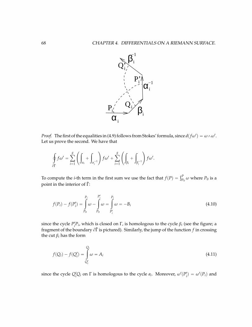
68 CHAPTER 4. DIFFERENTIALS ON A RIEMANN SURFACE.
−1
i
i
i
Qii
Q’i
P’i
P βα
α
β−1
i
Proof. The first of the equalities in (4.9) follows from Stokes’ formula, since dp fω1q “ ω^ω1.Let us prove the second. We have that
¿
BΓ
fω1 “gÿ
i“1
˜
ż
αi
`
ż
α´1i
¸
fω1 `gÿ
i“1
˜
ż
βi
`
ż
β´1i
¸
fω1.
To compute the i-th term in the first sum we use the fact that f pPq “şP
P0ω where P0 is a
point in the interior of Γ:
f pPiq ´ f pP1iq “
Piż
P0
ω´
P1iż
P0
ω “
Piż
P1i
ω “ ´Bi (4.10)
since the cycle P1iPi, which is closed on Γ, is homologous to the cycle βi (see the figure; afragment of the boundary BΓ is pictured). Similarly, the jump of the function f in crossingthe cut βi has the form
f pQiq ´ f pQ1iq “
Qiż
Q1i
ω “ Ai (4.11)
since the cycle Q1iQi on Γ is homologous to the cycle ai. Moreover, ω1pP1iq “ ω1pPiq and
4.1. HOLOMORPHIC DIFFERENTIALS 69
ω1pQ1iq “ ω1pQiq because the differential ω1 is single-valued on Γ. We have that
ż
αi
f pPiqω1pPiq `
ż
α´1i
f pP1iqω1pP1iq “
ż
αi
f pPiqω1pPiq ´
ż
αi
p f pPiq ` Biqω1pPiq
“ ´Bi
ż
αi
ω1pPiq “ ´BiA1i
where the minus sign appears because the edge a´1i occurs in BΓ with a minus sign.
Similarly,˜
ż
βi
`
ż
β´1i
¸
fω1 “ AiB1i.
Summing these equalities, we get (4.9). The lemma is proved.
We derive some important consequences for periods of holomorphic differentialsfrom the lemma 4.15. Everywhere we denote by α1, . . . , αg, β1, . . . , βg the canonical basisof cycles on Γ.
Corollary 4.16. . Letω be a nonzero holomorphic differential on Γ, and A1, . . . ,Ag, B1, . . . ,Bg itscorresponding periods with respect to the canonical homology basis α1 . . . , αg and β1 . . . , βg, then
=
˜ gÿ
i“1
AkBk
¸
ă 0. (4.12)
Proof. Take ω1 “ ω in the lemma 4.15. Then A1i “ Ai and B1i “ Bi for i “ 1, . . . , g. We havethat
i2
ż ż
Γω^ ω1 “
i2
ż ż
| f |2dz^ dz “ż ż
Γ| f |2dx^ dy ą 0.
Here z “ x` iy is a local parameter, and ω “ f pzqdz. In view of (4.9) this integral is equalto
i2
gÿ
k“1
AkBk ´ AkBk “ ´=
˜ gÿ
k“1
AkBk
¸
.
The corollary is proved.
Corollary 4.17. If all the α-periods of a holomorphic differential are zero, then ω “ 0.
This follows immediately from Corollary 4.16.
70 CHAPTER 4. DIFFERENTIALS ON A RIEMANN SURFACE.
Corollary 4.18. On a surface Γ of genus g there exists a basis ω1, . . . , ωg of holomorphic differ-entials such that
¿
α j
ωk “ δ jk, j, k “ 1, . . . , g. (4.13)
Proof. Let η1, . . . , ηg be an arbitrary basis of holomorphic differentials on Γ. The matrix
A jk “
¿
α j
ηk (4.14)
is nonsingular. Indeed, otherwise there are constants cl, . . . , cg such thatř
k A jkck “ 0.But then
ř
k ckηk “ 0, since this differential has zero a-periods. This contradicts theindependence of the differentials ηi, . . . , ηk.
ω j “
gÿ
k“1
Akjηk, j “ 1, . . . , g, (4.15)
where the matrix pAkjq is the inverse of the matrix pA jkq,ř
k AikAkj “ δi j, we get the desiredbasis. The corollary is proved.
A basis ω1, . . . , ωg satisfying the conditions (4.13) will be called a normal basis ofholomorphic differentials (with respect to a canonical basis of cycles α1, . . . , αg, β1, . . . , βgq
.
Corollary 4.19. Let ω1, . . . ωg be a normalized basis of holomorphic differentials, and let
B jk “
¿
β j
ωk, j, k “ 1, . . . , g. (4.16)
Then the matrix pB jkq is symmetric and has positive-definite imaginary part.
Proof. Let us apply the lemma 4.15 to the pair ω “ ω j and ω1 “ ωk. Then ω^ω1, Ai “ δi j,Bi “ Bi j, A1i “ δik, B1i “ Bik. By (4.9) we have that
0 “ÿ
i
pδi jBik ´ δikBi jq “ pB jk ´ Bkjq.
The symmetry is proved. Next, we apply Corollary 4.16 to the differentialřg
j“1 x jω j
where all the coefficients x1, . . . , xg are real. We have that Ak “ xk, Bk “ř
j x jBkj whichimplies
=pÿ
k
xk
ÿ
j
x jBkjq “ÿ
k, j
=pBkjqxkx j ă 0.
The lemma is proved.
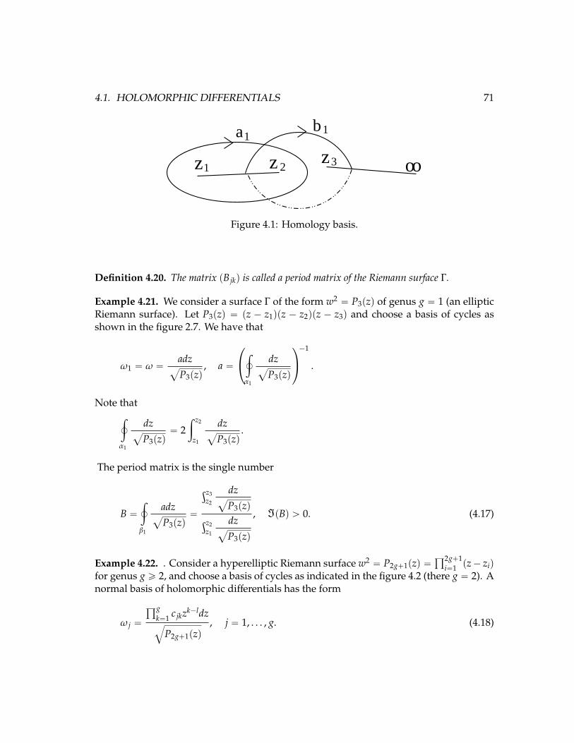
4.1. HOLOMORPHIC DIFFERENTIALS 71
ooz z
b
z
a
1 2 3
11
Figure 4.1: Homology basis.
Definition 4.20. The matrix pB jkq is called a period matrix of the Riemann surface Γ.
Example 4.21. We consider a surface Γ of the form w2 “ P3pzq of genus g “ 1 (an ellipticRiemann surface). Let P3pzq “ pz ´ z1qpz ´ z2qpz ´ z3q and choose a basis of cycles asshown in the figure 2.7. We have that
ω1 “ ω “adz
a
P3pzq, a “
¨
˝
¿
α1
dza
P3pzq
˛
‚
´1
.
Note that¿
α1
dza
P3pzq“ 2
ż z2
z1
dza
P3pzq.
The period matrix is the single number
B “¿
β1
adza
P3pzq“
şz3z2
dza
P3pzqşz2
z1
dza
P3pzq
, =pBq ą 0. (4.17)
Example 4.22. . Consider a hyperelliptic Riemann surface w2 “ P2g`1pzq “ś2g`1
i“1 pz´ ziq
for genus g ě 2, and choose a basis of cycles as indicated in the figure 4.2 (there g “ 2). Anormal basis of holomorphic differentials has the form
ω j “
śgk“1 c jkzk´ldzb
P2g`1pzq, j “ 1, . . . , g. (4.18)
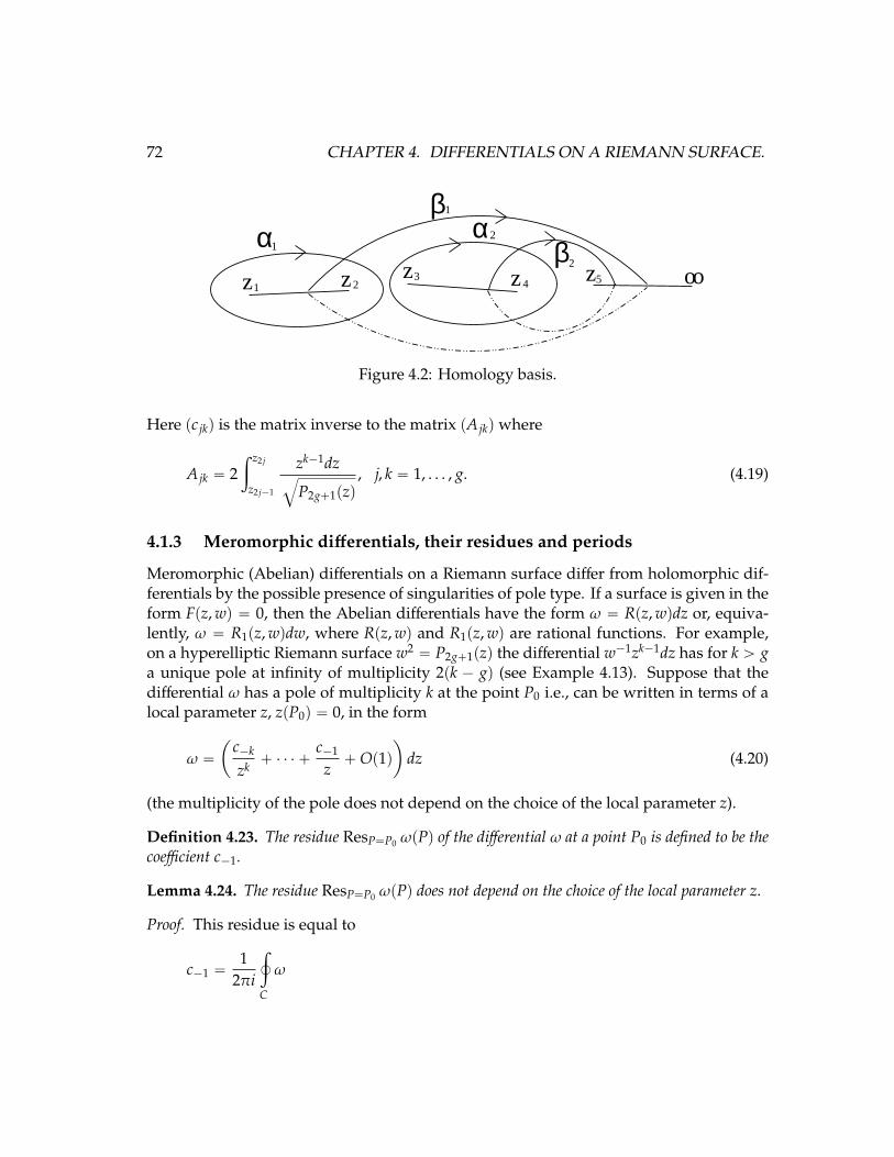
72 CHAPTER 4. DIFFERENTIALS ON A RIEMANN SURFACE.
oozz zz z
βα
βα5
1 23
4
1
1
2
2
Figure 4.2: Homology basis.
Here pc jkq is the matrix inverse to the matrix pA jkqwhere
A jk “ 2ż z2 j
z2 j´1
zk´1dzb
P2g`1pzq, j, k “ 1, . . . , g. (4.19)
4.1.3 Meromorphic differentials, their residues and periods
Meromorphic (Abelian) differentials on a Riemann surface differ from holomorphic dif-ferentials by the possible presence of singularities of pole type. If a surface is given in theform Fpz,wq “ 0, then the Abelian differentials have the form ω “ Rpz,wqdz or, equiva-lently, ω “ R1pz,wqdw, where Rpz,wq and R1pz,wq are rational functions. For example,on a hyperelliptic Riemann surface w2 “ P2g`1pzq the differential w´1zk´1dz has for k ą ga unique pole at infinity of multiplicity 2pk ´ gq (see Example 4.13). Suppose that thedifferential ω has a pole of multiplicity k at the point P0 i.e., can be written in terms of alocal parameter z, zpP0q “ 0, in the form
ω “
ˆ
c´k
zk` ¨ ¨ ¨ `
c´1
z`Op1q
˙
dz (4.20)
(the multiplicity of the pole does not depend on the choice of the local parameter z).
Definition 4.23. The residue ResP“P0 ωpPq of the differential ω at a point P0 is defined to be thecoefficient c´1.
Lemma 4.24. The residue ResP“P0 ωpPq does not depend on the choice of the local parameter z.
Proof. This residue is equal to
c´1 “1
2πi
¿
C
ω
4.1. HOLOMORPHIC DIFFERENTIALS 73
where C is an arbitrary small contour encircling P0. The independence of this integral onthe choice of the local parameter is obvious. The lemma is proved.
Theorem 4.25 (The Residue Theorem). . The sum of the residues of a meromorphic differentialω on a Riemann surface, taken over all poles of this differential, is equal to zero.
Proof. Let P1, . . . ,PN be the poles of ω. We encircle them by small contours C1, ...,CN suchthat
Resω “1
2πi
¿
Ci
ω, i “ 1, . . . ,N,
(the contours Ci run in the positive direction), and cut out the domains bounded byC1, . . . ,CN from the surface Γ. This gives a domain Γ1 with oriented boundary of theform BΓ1 “ ´C1 ´ ¨ ¨ ¨ ´ CN (the sign means reversal of orientation). The differential ω isholomorphic on Γ1. By Stokes’ formula,
Nÿ
j“1
ResP jω “
12πi
Nÿ
j“1
¿
C j
ω “ ´1
2πi
¿
BΓ1
ω “ ´1
2πi
ż ż
Γ1dω “ 0,
since dω “ 0. The theorem is proved.
We present the simplest example of the use of the residue theorem: we prove thatthe number of zeros of a meromorphic function is equal to its number of poles (countingmultiplicity). Let P1, . . . ,Pk, be the zeros of the meromorphic function f , with multiplicitiesm1, . . . ,mk a nd let Q1, ...,Ql be the poles of this function, with multiplicities n1, . . . ,nk.Consider the logarithmic differential dpln f q. This is a meromorphic differential on Γwith simple poles at P1, . . . ,Pk with residues m1, . . . ,mk and at the points Q1, . . . ,Ql withresidues ´n1, . . . ,´nl. By the residue theorem: m1 ` ¨ ¨ ¨ `mk ´ n1 ´ ¨ ¨ ¨ ´ nk “ 0 , whichmeans that the assertion to be proved is valid. One more example. For any elliptic functionf pzq on the torus T2 “ Ct2mω` 2nω1u the residues at the poles are defined with respectto the complex coordinate z (in C). These are the residues of the meromorphic differentialf pzqdz, since dz is holomorphic everywhere. Conclusion: the sum of the residues of anyelliptic function (over all poles in a lattice parallelogram) is equal to zero. We formulatean existence theorem for meromorphic differentials on a Riemann surface Γ (see [?] for aproof).
Theorem 4.26. Suppose that P1, . . . ,PN are points of a Riemann surface Γ and z1, . . . , zN arelocal parameters centered at these points, zipPiq “ 0, and the collection of principal parts is
¨
˝
cpiq´ki
zkii
` ¨ ¨ ¨ `cpiq´1
zi
˛
‚dzi, i “ 1, . . . ,N. (4.21)

74 CHAPTER 4. DIFFERENTIALS ON A RIEMANN SURFACE.
Assume the condition
Nÿ
i“1
ci´1 “ 0. (4.22)
Then there exists on Γ a meromorphic differential with poles at the points P1, . . . ,PN, and principalparts (4.21).
Any meromorphic differential can be represented as the sum of a holomorphic differ-ential and the following elementary meromorphic differentials.
1. Abelian differential of the second kind ΩnP has a unique pole of multiplicity n` 1 at
P and a principal part of the form
ΩnP “
ˆ
1zn`1
`Op1q˙
dz (4.23)
with respect to some local parameter z, zpPq “ 0, n “ 1, 2, . . . .
2. An Abelian differential of the third kind ΩPQ has a pair of simple poles at the pointsP and Q with residues `1 and ´1 respectively.
Example 4.27. We construct elementary Abelian differentials on a hyperelliptic Riemannsurface w2 “ P2g`1pzq. Suppose that a point P which is not a branch point takes the form
P “ pa,wa “b
P2g`1paqq. An Abelian differential of the second kind Ωp1qP has the form
Ωp1qP “
˜
w` wa
pz´ aq2´
P12g`1paq
2wapz´ aq
¸
dz2w
(4.24)
(with respect to the local parameter z-a). The differentials ΩpnqP can be obtained as follows:
ΩnP “
1n!
dn´1
dan´1Ω1
P. (4.25)
If P “ pzi, 0q is one of the branch points, then
ΩnP “
dz2pz´ ziqk`1
for n “ 2k, ΩnP “
dz2pz´ ziqk`1w
for n “ 2k` 1. (4.26)
Finally, if P “ 8, then
ΩpnqP “ ´
12
zk´1dz for n “ 2k, ΩnP “ ´
12
zg`k´1 dzw
for n “ 2k` 1. (4.27)
4.1. HOLOMORPHIC DIFFERENTIALS 75
We now construct differentials of the third kind. Suppose that the point P and Q have the
form P “ pa,wa “b
P2g`1paqq and Q “ pb,wb “b
P2g`1pbqq. Then
ΩPQ “
ˆ
w` wa
z´ a´
w` wb
z´ b
˙
dz2w
(4.28)
If Q “ `8 then
ΩPQ “w` wa
z´ adz2w. (4.29)
Accordingly, we see that for a hyperelliptic Riemann surface it is possible to represent allthe Abelian differentials without appealing to Theorem 4.26.
Exercise 4.28: Deduce from Theorem 4.26 that a Riemann surface Γ of genus 0 is rational.Hint. Show that for any points P, Q P Γ the function f “ exp
ş
ΩPQ is single valued andmeromorphic on Γ and gives a biholomorphic isomorphism f : Γ Ñ CP1.
The period of a meromorphic differential ω along the cycle γ is defined if the cycledoes not pass through poles of this differential. The period
ş
γω depends only on thehomology class of γ on the surface Γ, with the poles of ω with nonzero residue deleted.For example, the periods of the differential ΩPQ of the third kind along a cycle not passingthrough the points P and Q are determined to within integer multiples of 2πi. In speakingof the periods of meromorphic differentials we shall assume that the cycles do not passthrough the poles of the differential, and we also recall that the dependence of the periodon the homology class of Γ is not single-valued (for differentials of the third kind).
Lemma 4.29. Suppose that the differentials Ω1 and Ω2 on a Riemann surface Γ have the samepoles and principal parts, and the same periods with respect to the cycles α1, . . . , αg, β1, . . . , βg.Then these differentials coincide.
Proof. The differenceω1´ω2 is a holomorphic differential that has zero α-periods. There-fore, it is identically zero (see Lecture 4.1.2). The lemma is proved.
Definition 4.30. A meromorphic differential ω is said to be normalized with respect to a basis ofcycles α1, . . . , αg, β1, . . . , βg if it has zero α-periods.
Any meromorphic differentialω can be turned into a normalized differential by addinga holomorphic differential
řgk“1 ckωk. Indeed the condition that Ω “ ω `
ř
ckωk isnormalised, namely
ż
α j
ω`gÿ
k“1
ck
ż
α j
ωk “ 0, j “ 1, . . . , g,
76 CHAPTER 4. DIFFERENTIALS ON A RIEMANN SURFACE.
defines the constants c1, . . . , cg uniquely.By Lemma 4.29, a normalized meromorphic differential is uniquely determined by its
poles and by the principal parts at the poles. In what follows we assume that meromorphicdifferentials are normalized. We obtain formulas that will be useful for the β-periods ofsuch differentials by arguments like those in the proof of Lemma 4.15.
Lemma 4.31. The following formulas hold for the β-periods of normalized differentials ΩpnqP and
ΩPQ
¿
βk
ΩpnqP “ 2πi
1n!
dn´1
dzn´1ψipzq|z“0, k “ 1, . . . , g, n “ 1, 2, . . . , (4.30)
where z is a particular local parameter in a neighborhood of P, zpPq “ 0, and the functions ψkpzqare determined by the equality ωk “ ψkpzqdz and ω1, . . . , ωg is a normalized basis of holomorphicdifferentials with respect to the canonical homology basis α1, . . . , αg, β1, . . . , βg,
¿
βk
ΩPQ “ 2πiż P
Qωk, i “ 1, . . . , g, (4.31)
where the integration from Q to P in the last integral does not intersect the cycles α1, . . . , αg,β1, . . . , βg.
Proof. We encircle the point P with a small circle C oriented anti-clockwise; deleting theinterior of this circle from the surface Γ, we get a domain Γ1 with BΓ1 “ ´C. Let us applythe arguments of Lemma 4.15 to the pair of differentials ω “ ωk, ω1 “ Ω
pnqP . Denote by ui
the primitive
ukpQq “ż Q
P0
ωk (4.32)
which is single-valued on the Poincare’ polygon Γ of the surface Γ. We have that
0 “ż ż
Γ1ω^ ω1 “
ż
BΓ1ukΩ
pnqP “
gÿ
j“1
pA jB1j ´ A1jB jq ´
¿
C
ukΩpnqP (4.33)
(the boundary BΓ1 differs from the boundary BΓ by p´Cqq. Here the α and β-periods of ωkand ΩN
P have the form
A j “ δkj, B j “ Bkj, A1j “ 0, B1j “¿
β j
ΩpnqP .
4.1. HOLOMORPHIC DIFFERENTIALS 77
From this,
¿
βk
ΩpnqP “
¿
C
ukΩpnqP “ 2πi Res
PpukΩ
pnqP q “ 2πi Res
z“0
„ˆż P
P0
`
ż z
0ψkpτqdτ
˙
dzzn`1
(4.34)
Computation of the residue on the right-hand side of this equality leads to (4.30).We now prove (4.31). Let C and C1 small circles around P and Q respectively. Deleting theinterior of this circles from the surface Γ, we get a domain Γ1 with BΓ1 “ ´C´ C1. Let usapply the arguments of Lemma 4.15 to the pair of differentials ω “ ωk, ω1 “ ΩPQ. Denoteby ui the primitive of ωi. By analogy with (4.33) and (4.34) we have that
¿
βk
ΩPQ “ 2πi¿
C
ukΩPQ ` 2πi¿
C1
ukΩPQ
Since the differential ΩPQ has a simple pole in P and Q with residue ˘1 respectively, theabove integrals are equal to
¿
βk
ΩPQ “ ukpPq ´ ukpQq “ż P
P0
ωk ´
ż Q
P0
ωk “
ż P
Qωk
where we assume that the point P0 lies in the interior of Γ1. The lemma is proved.
Exercise 4.32: Prove the following equality, which is valid for any quadruple of distinctpoints P1, . . . ,P4 on a Riemann surface:
ż P1
P2
ΩP3P4 “
ż P3
P4
ΩP1P2 . (4.35)
Exercise 4.33: Consider the series expansion of the differentials ΩpnqP in a neighborhood
of the point P
ΩpnqP “
¨
˝
1zn`1
`
8ÿ
j“0
cpnqj z j
˛
‚dz. (4.36)
Prove the following symmetry relations for the coefficients cpkqj :
kcpkqj´1 “ jcp jqk´1, k, j “ 1, 2 . . . . (4.37)
78 CHAPTER 4. DIFFERENTIALS ON A RIEMANN SURFACE.
Exercise 4.34: Prove that a meromorphic differential of the second kind ω is uniquelydetermined by its poles, principal parts, and the real normalization condition
=
¿
γ
ω “ 0 (4.38)
for any cycle γ. Formulate and prove an analogous assertion for differentials of the thirdkind (with purely imaginary residues).
Elliptic curve and elliptic functions
Let’s come back to the example 4.21 and consider the function (”elliptic integral”)
upPq “ż P
P0
ω1, (4.39)
which is single-valued and holomorphic on the surface Γ which is obtained by cuttingΓ along the cycles α1 and β1. This function is not single-valued on Γ. When the pathof integration in the integral (4.39) is changed, the integral changes according to the lawupPq Ñ upPq `
ş
γωi where γ is a closed contour (cycle). Decomposing it with respect tothe basis of cycles, γ “ mα1 ` nβ1, m and n integers we rewrite the last formula in theform
upPq Ñ upPq `m` Bn, =pBq ą 0. (4.40)
We define the two-dimensional torus T2 as the quotient of the complex plane C “ R2 bythe integer lattice generated by the vectors 1 and B,
T2 “ Ct2πim` Bn | m,n P Zu (4.41)
(the vectors 1 and B are independent over R because =pBq ą 0). The torus T2 is aone-dimensional compact complex manifold. By (4.40) the function upPq unambiguouslydefines a mapping Γ Ñ T2. It is holomorphic everywhere on Γ: du “ ω and du vanishesnowhere (verify!). It is easy to see that this is an isomorphism. The meromorphic functionson the Riemann surface Γ are thereby identified with the so-called elliptic functions – themeromorphic functions on the torus T2. The latter functions can be regarded as doublyperiodic meromorphic functions of a complex variable. The absence of nonconstantholomorphic functions on Γ (see Lecture 3) leads to the well-known assertion that thereare no nonconstant doubly periodic holomorphic functions. For comparison with thestandard notation of the theory of elliptic functions we note that usually B is denotedwith the letter τ and =τ ą 0. We give the construction of the mapping T2 Ñ Γ inverse to
4.1. HOLOMORPHIC DIFFERENTIALS 79
(4.39). Letω1 andω2 be two complex numbers linearly independent over the real numbersand consider the torus T2 defined as
T2 “ CL, L “ t2mω1 ` 2nω2 | m,n P Zu. (4.42)
The Weierstrass elliptic function, ℘puq, u P C is defined by
℘puq “1u2 `
ÿ
ωPLzt0u
„
1pu´ ωq2
´1ω2
(4.43)
It is not hard to verify that the function ℘puq converges absolutely and uniformly on com-pact sets not containing nodes of the period lattice. Therefore, it defines a meromorphicfunction of u having double poles at the lattice nodes. Its derivative ℘1puq can be obtainedby differentiating the series term by term ( check!)
℘1puq “ ´2ÿ
ωPL
1pu´ ωq3
.
The function ℘puq is obviously doubly periodic: ℘pu ` 2mω1 ` 2nω2q “ ℘puq, m,n P Z.The Laurent expansions of the functions℘puq and℘1puq have the following forms as u Ñ 0
℘puq “1u2 `
g2u2
20`
g3u4
28` . . . , (4.44)
℘1puq “ ´2u3 `
g2u10
`g3u3
7` . . . , (4.45)
where
g2 “ 60ÿ
ωPLzt0u
ω´4
g2 “ 140ÿ
ωPLzt0u
ω´6,(4.46)
(verify!). This gives us that the Laurent expansion of the function p℘1q2 ´ 4℘3 ` g2℘` g3has the form Opuq as z Ñ 0. Hence, this doubly periodic function is constant, and thusequal to zero. Conclusion: the Weierstrass function ℘puq satisfies the differential equation
p℘1q2 “ 4℘3 ´ g2℘´ g3. (4.47)
Proposition 4.35. The function ℘ : CzL Ñ C is surjective. If
℘puq “ ℘pu0q, then u P L˘ u0. (4.48)
80 CHAPTER 4. DIFFERENTIALS ON A RIEMANN SURFACE.
Proof. For any c P C consider the function f puq “ ℘puq ´ c. This function is meromorphicwith a double pole on the lattice points. Consider the parallelogram
Π :“ tξ` 2sω1 ` 2tω2, s, t P r0, 1su.
Since the function f has only a double pole in Π, it has two zeros counting multiplicity.Let u0 be one of the two zeros, f pu0q “ ℘pu0q ´ c “ 0. Since ℘p´uq “ ℘puq, it followsthat 0 “ f p´u0q “ ℘p´u0q ´ c and this shows that the function ℘puq is surjective. Fromthe above argument and the periodicity of ℘, it follows that for any u P L ˘ u0, one has℘puq “ ℘pu0q.
Let us now consider the curve
ΓL :“ trX : Y : Zs P P2 |ZY2 “ 4X3 ´ g2XZ2 ´ g3Z3u (4.49)
Lemma 4.36. The curve ΓL is non singular.
Proof. Consider the affine curve (4.47). By the periodicity properties of ℘puq one has
℘1pu` 2ω1q “ ℘1puq
which is true in particular for u “ ´ω1 so that ℘1pω1q “ ℘1p´ω1q. Since ℘1puq is odd itfollows that
℘1pω1q “ 0.
Repeating the same reasoning for ω2 one has
℘1pω2q “ 0, ℘1pω2 ` ω1q “ 0.
Using (4.47) the zeros of the polynomial 4℘3puq´ g2℘puq´ g3 are given by u “ ω1, u “ ω2
and u “ ω1 ` ω2 so that one has
4℘3puq ´ g2℘puq ´ g3 “ 4p℘puq ´ ℘pω1qqp℘puq ´ ℘pω2qqp℘puq ´ ℘pω1 ` ω2qq.
By proposition 4.35 the values ℘pω1q, ℘pω2q and ℘pω1 ` ω2q are distinct so that the curve(4.47) is non singular.
The following theorem can be proved as an exercise
Theorem 4.37. The map
φ : T2 Ñ ΓL
defined by
φpu` Lq “"
r℘puq : ℘1puq : 1s u P CzLr0 : 1 : 0s u P L, (4.50)
is biholomorphic.
4.1. HOLOMORPHIC DIFFERENTIALS 81
In particular the map (4.50) is the inverse of the map (4.39). We observe that fromlemma 4.36 the discriminant ∆pω1, ω2q of the curve (4.47) is different from zero, namely
∆pω1, ω2q “ g32pω
1, ω2q ´ 27g23pω
1, ω2q , 0
furthermore under the dilatation ω1 Ñ λω1 and ω2 Ñ λω2 the discriminant scales as
∆pλω1, λω2q “1λ12
∆pω1, ω2q.
In particular, choosing λ “ 12ω1 and defining τ “
2ω2
2ω1, with =pω2ω1q ą 0, we obtain that
g2 “ g2pτq, and g3 “ g3pτq, ∆ “ ∆pτq with τ P H, H :“ tτ P C, =τ ą 0u. Regarding theWeierstrasse ℘ function it is easy to check that
℘pλu;λω1, λω2q “1λ2℘pu, ;ω
1, ω2q
so that choosing λ “ 12ω1 one can consider the Weierstrasse function normalised as
℘pu; τq “1u2 `
ÿ
m,nPZ,pm,nq,p0,0q
„
1pu´m´ nτq2
´1
pm` nτq2
, u “u
2ω1.
Exercise 4.38: Show that
℘pu
cτ` d;
aτ` bcτ` d
q “ pcτ` dq2℘pu; τq,ˆ
a bc d
˙
P SLp2,Zq. (4.51)
Definition 4.39. The Klein J function J :HÑ C is defined as
Jpτq “ 1728g2pτq3
∆pτq. (4.52)
The Klein J function is an an analytic function fromH to C. The choice of the number1728 is due to the fact that defining q “ e2πiτ the expansion of J as q Ñ 0 takes the form
Jpqq “1q` 744` 196884q` 21493760q2 ` . . .
namely all the coefficients of the expansion are integers. We consider the action of themodular group
PSLp2,Zq “ SLp2,ZqtI,´Iu
82 CHAPTER 4. DIFFERENTIALS ON A RIEMANN SURFACE.
namely the set of 2ˆ 2 matrices with integer entries and determinant equal to one wherethe matrices A and ´A are identified. Such group has two generators
τÑ τ` 1, τÑ ´1τ.
In order to determine isomorphism classes of elliptic curves given by 4.49), the followinglemma and theorem will be usefull.
Lemma 4.40. Let τ and τ1 PH. Then
Jpτ1q “ Jpτq.
if and only if
τ1 “aτ` bcτ` d
,
ˆ
a bc d
˙
P PSLp2,Zq. (4.53)
Proof. From the definition one has
g2pτ1q “ 60
ÿ
m,nPZ,pm,nq,p0,0q
¨
˚
˚
˝
1
m` naτ` bcτ` d
˛
‹
‹
‚
4
“ 60pcτ` dq4ÿ
m1,n1PZ,pm1,n1q,p0,0q
1pm1 ` n1τq4
“ pcτ` dq4g2pτq.
In the same way we obtain
g3pτ1q “ pcτ` dq6g3pτq
so that
Jpτ1q “ 1728g3
2pτ1q
g32pτ
1q ´ 27g23pτ
1q“ 1728
pcτ` dq12g32pτq
pcτ` dq12pg32pτq ´ 27g2
3pτq“ Jpτq.
Viceversa, let us assume that Jpτq “ Jpτ1q “ µ. Suppose µ , 0 and µ , 1728. Then
µ´ 1728 “ 172827g2
3pτq
∆pτq“ 1728
27g23pτ
1q
∆pτ1q
so that
µ
µ´ 1728“
27g23pτ
1q
g32pτ
1q“
27g23pτq
g32pτq
4.1. HOLOMORPHIC DIFFERENTIALS 83
which shows thatˆ
g3pτq
g3pτ1q
˙2
“
ˆ
g2pτq
g2pτ1q
˙3
.
Defining σ2 :“g2pτq
g2pτ1q
g3pτ1q
g3pτq, it is straightforward to obtain the identity
σ4 “
ˆ
g2pτq
g2pτ1q
g3pτ1q
g3pτq
˙2
“g2pτ1q
g2pτq
and
σ6 “g3pτ1q
g3pτq.
Therefore the curves defined by w2 “ 4z3´ g2pτqz´ g3pτq and y2 “ 4x3´ g2pτ1qx´ g3pτ1qare isomorphic. Indeed the dilatation
x “ zσ2, y “ wσ3
maps one curve into the other one. Therefore the two tori defined by the above twocurves are isomorphic. By theorem 1.43 it follows that their corresponding periods τand τ1 are related by a modular transformation (4.53). In the case µ “ 1728 one has
g3pτq “ g3pτ1q “ 0. In this case defining σ in such a way that σ4 “g2pτ1q
g2pτqone can prove
the statement in a similar way. For the case µ “ 0 one has g2pτq “ g2pτ1q “ 0. In this
case defining σ in such a way that σ6 “g3pτ1q
g3pτqone can prove the statement in a similar
way.
The above lemma shows that the Klein J function is a modular function of weightzero. We recall that an analytic function f :HÑ C is a modular function of weight k withrespect to the modular group PSLp2,Zq if
fˆ
aτ` bcτ` d
˙
“ pcτ` dqk f pτq,ˆ
a bc d
˙
P PSLp2,Zq.
Remark 4.41. The upper half space H can be naturally identified with the Teichmullerspace Tp1, 0q of compact surfaces of genus one. The quotientHPSLp2,Zq is the modulispace of Riemann surfaces of genus one. Below we will see that this moduli space can beidentified with sCwith three marked points modulo the permutation group S3.
84 CHAPTER 4. DIFFERENTIALS ON A RIEMANN SURFACE.
Combining theorem 1.43 and lemma 4.40 we conclude that
Theorem 4.42. Given two lattices L “ tn ` mτ, m,n P Zu and L1 “ tn ` mτ1, m,n P Zuwith τ, τ1 PH, the tori
CL, CL1
are isomorphic if and only if
Jpτq “ Jpτ1q.
Doing some algebra we can express the Klein J invariant using the branch points℘pτ2q, ℘p12q and ℘p 1`τ
2 q of the elliptic curve (4.47). For simplicity we define
e1 “ ℘pτ2q, e2 “ ℘p12q, e3 “ ℘p1` τ
2q. (4.54)
It is easy to check that
∆ “ 16pe2´ e1q2pe3´ e1q
2pe3´ e2q2, g2 “
43`
pe2 ´ e1q2 ´ pe3 ´ e1qpe2 ´ e1q ` pe3 ´ e1q
2˘
so that Jpτq can be written in the form
Jpτq “ 256
ˆ
1´e3 ´ e1
e2 ´ e1`pe3 ´ e1q
2
pe2 ´ e1q2
˙3
pe3 ´ e1q2
pe2 ´ e1q2
pe3 ´ e2q2
pe2 ´ e1q2
. (4.55)
Introducing the function λ :HÑ Czt0, 1u
λ “e3 ´ e1
e2 ´ e1“℘p 1`τ
2 q ´ ℘pτ2q℘p12q ´ ℘pτ2q
(4.56)
and the function j : Czt0, 1u Ñ C defined as
jpλq “ 256p1´ λ` λ2q3
λ2p1´ λq2(4.57)
it follows that the Klein J invariant is the composition of the maps
J “ j ˝ λ.
4.1. HOLOMORPHIC DIFFERENTIALS 85
Remark 4.43. Since the function J as defined in (4.52) is invariant under the action of thepermutation group S3 on e1, e2 and e3, such invariance must be preserved for the functionjpλq. Indeed one has the following relations between the action of S3 on e1, e2 and e3 andtransformations of λ:
123 Ñ 213 then λÑ 1´ λ, 123 Ñ 321 then λÑλ
1´ λ, 123 Ñ 132 then λÑ
1λ
123 Ñ 231 then λÑ1
1´ λ, 123 Ñ 312 then λÑ 1´
1λ
and the function jpλq is invariant under the above five transformations of λ (six includingthe identity).
The curve w2 “ 4pz´ e1qpz´ e2qpz´ e3q is mapped under the linear transformation
x “z´ e1
e2 ´ e1, y “
w
2pe2 ´ e1q32
to the curve
y2 “ xpx´ 1qpx´ λq.
So using the j-invariant (4.57), we have the following corollary.
Corollary 4.44. Two curves y2 “ xpx´ 1qpx´ λq and y2 “ xpx´ 1qpx´ λ1q are isomorphic ifand only jpλq “ jpλ1q.
We will see later that any Riemann surface of genus one can be realised as a doublecovering of the sphere branched over four points e1, e2, e3 and 8. We can use a lineartransformation to map the points e1, e2 and e3 to 0, 1 and λ respectively. Any other lineartransformation obtained from the permutation of the points e1, e2 and e3 will give anisomorphic Riemann surface. So we can identify the moduli space of genus one Riemannsurface as the quotient pCzt0, 1uqS3. In remark (4.41) we identify the moduli space ofRiemann surfaces of genus one with HPSLp2,Zq. Below we are going to sketch anargument which shows that the spaces
pCzt0, 1uqS3 and HPSLp2,Zq
are isomorphic.
Lemma 4.45. The map λ : H Ñ Czt0, 1u is a universal covering of Czt0, 1u. This map isinvariant under the action of the subgroup Γ2 Ă PSLp2,Zq
Γ2 “
"ˆ
a bc d
˙
P PSLp2,Zq | a ” d ” 1 pmod 2q, b ” c ” 0 pmod 2q*
.
86 CHAPTER 4. DIFFERENTIALS ON A RIEMANN SURFACE.
Proof. Let us consider λpτ1q and use the relation (4.51)
λpτ1q “℘pτ
1`12 ; τ1q ´ ℘pτ
1
2 ; τ1q
℘p 12 ; τ1q ´ ℘pτ12 ; τ1q
“℘p 1
2pb` d` pa` cqτq; τq ´ ℘p 12paτ` bq; τq
℘p d`cτ2 ; τq ´ ℘p1
2paτ` bq; τq.
It is straightforward to check that λpτ1q “ λpτq if and only if the modular transformationbelongs to Γ2.
Remark 4.46. The group Γ2 is the group of deck transformations of the covering λ : HÑ
Czt0, 1u, namely the set of homeomorphism f : H Ñ H preserving the fibers of thecovering. Such group is isomorphic to the fundamental group of Czt0, 1u and therefore[14]
HΓ2 » Czt0, 1u.
Furthermore, the following identity is satisfied [12] PSLp2,ZqΓ2 » S3. Namely thequotient of the modular group under the group Γ2 is isomorphic to the group of permu-tation S3. The above identity and the lemma 4.45 explain the identification of the spacespCzt0, 1uqS3 and HPSLp2,Zq .
Exercise 4.47: Prove that any elliptic function with period lattice t2mω2 ` 2nω1u can berepresented as a rational function of ℘pzq and ℘1pzq.
Exercise 4.48: Show that if τ is pure imaginary then the branch points e1, e2 and e3 arereal.
Exercise 4.49: Consider the curve
Γ :“ tpz,wq P P2 | w2 “ zpz´ 1qpz´ λqu
with 0 ď λ ď 1 and consider the lattice L “ t2mω1 ` 2nω2, m,n P Zuwhere
ż 0
8
dzw“ L` ω2,
ż 1
8
dzw“ L` ω1 ` ω2,
ż λ
8
dzw“ L` ω1.
Show that the curve Γ is isomorphic to the curve w2 “ 4z3 ´ g2z´ g3 where g2 and g3 aredefined in (4.46).
Exercise 4.50: Consider the Korteweg-de Vries (KdV) equation
ut “ 6uux ´ uxxx (4.58)
4.1. HOLOMORPHIC DIFFERENTIALS 87
(here u “ upx, tq, and ut stands for the derivative with respect to t, and ux for derivativewith respect to x. Show that any (complex) periodic solution of it with the form of atraveling wave has the form
upx, tq “ upx´ ctq “ 2℘px´ ct´ x0q ´c6, (4.59)
where the Weierstrass function℘ corresponds to some elliptic curve (4.49), and the velocityc and the phase x0 are arbitrary.
Exercise 4.51: (see [8]). Look for a solution of the KdV equation in the form
upx, tq “ 2℘px´ x1ptqq ` 2℘px´ x2ptqq ` 2℘px´ x3ptqq. (4.60)
Derive for the functions x jptq the system of differential equations
:x j “ 12ÿ
k, j
℘px j ´ xkq, j “ 1, 2, 3, (4.61)
and its integralsÿ
k, j
℘1px j ´ xkq “ 0, j “ 1, 2, 3. (4.62)
Integrate this system in quadratures.
We define the Weierstrass ζ and σ functions (which are useful in the theory of ellipticfunctions) from the conditions
ζ1pzq “ ´℘pzq,σ1pzqσpzq
“ ζpzq. (4.63)
The series expansion of ζpzq has the form
ζpzq “1z`
ÿ
ωPLzt0u
„
1z´ ω
`1ω`
zω2
. (4.64)
This function has simple poles at the nodes of the period lattice. The function σpzq isentire. It has simple zeros at the nodes of the period lattice and can be expanded in theinfinite product
σpzq “ zź
ωPLzt0u
"
´
1´zω
¯
exp„
zω`
z2
2ω2
*
(4.65)
88 CHAPTER 4. DIFFERENTIALS ON A RIEMANN SURFACE.
The functions ζpzq and σpzq are not elliptic; under a translation of the argument by a vectorof the period lattice they transform according to the law
ζpz` 2mω1 ` 2nω2q “ ζpzq ` 2mη` 2nη1, η “ ζpω1q, η1 “ ζpω2q, (4.66)σpz` 2ω1q “ σpzq expr2ηpz` ω1qs, σpz` 2ω2q “ ´σpzq expr2η1pz` ω2qs (4.67)
where η and η1 are constants depending on the period lattice.
Exercise 4.52: Prove the following identity:
σpu` vqσpu´ vqσ2puqσ2pvq
“ ℘puq ´ ℘pvq. (4.68)
Other properties of the functions,℘, ζ and σ and of other elliptic functions as well, canbe found, for example, in the texts [2] and [7], or in the handbook [3].
4.1.4 The Jacobi variety, Abel’s theorem
Let e1, . . . , eg be the standard basis in the space Cg, e j “ p0, . . . , 1, . . . , 0q, with one on thej-entry. Given 2g row vectors λk P C
g, k “ 1, . . . , 2g, with λk “řg
j“1 λkje j, we constructthe 2gˆ g matrix Λ having in the k-row the vector λk
Λkj “ pλkq j. (4.69)
The matrix Λ generates a lattice in Cg of maximal rank, if its row vectors are linearlyindependent over the real numbers.
Consider in Cg the integer period lattice L generated by the vectors (4.69). The vectorsin this lattice can be written in the form
L “ tv P Cg | v “2gÿ
k“1
mkλk, pm1, . . . ,m2gq P Z2gu (4.70)
We assume that L generates a lattice of maximal rank in Cg. Then the quotient of Cg bythis lattice is the 2g-dimensional torus
T2g “ CgL (4.71)
namely a g-dimensional complex manifold. Changing the basis in Cg, namely ek Ñ ekM,with M P GLpg,Cq, the matrix Λ Ñ ΛM. Furthermore, the same lattice is given by vectorspλ1, . . . , λ2gqwith
λk “
2gÿ
k“1
nkjλ j
4.1. HOLOMORPHIC DIFFERENTIALS 89
with N “ tnkju2gk, j“1 P SLp2g,Zq. Therefore Λ Ñ NΛ. Summarizing, two matrices Λ and
Λ represent the same torus if
Λ “ NΛM, M P GLpg,Cq, N P SLp2g,Zq. (4.72)
If we assume that the lattice generated by Λ has maximal rank, we can always chooseΛ in such a way that Λ “ p2πiΛ1,Λ2q with Λ1 P GLpg,Cq. Therefore, by (4.72) the twomatrices Λ and ΛΛ´1
1 “ p2πiIg,Λ2Λ´11 q with Ig the g-dimensional identity, represent the
same torus.
Lemma 4.53. The matrices
Λ “ pIg,Λ2q, Λ “ pIg, Λ2q
represent the same torus if
Λ2 “ pcIg ` dΛ2qpaIg ` bΛ2q´1,
ˆ
a bc d
˙
P SLp2g,Zq
with a, b, c, d gˆ g matrices.
The proof of the lemma follows immediately from (4.72).Let B “ pB jkq be an arbitrary symmetric g ˆ g matrix with positive-definite imagi-
nary part (as shown in Lecture 4.1.2, the period matrices of Riemann surfaces have thisproperty). We consider the vectors
e1, . . . , eg, e1B, . . . , egB. (4.73)
Lemma 4.54. The vectors (4.73) are linearly independent over R.
Proof. Assume that these vectors are dependent over R:
pρ1e1 ` ¨ ¨ ¨ ` ρgegq ` pµ1e1 ` ¨ ¨ ¨ ` µgegqB “ 0, ρi, µ j P R.
Separating out the real part of this equality we get that =ppµ1e1 ` ¨ ¨ ¨ ` µgegqBq “ 0.But the matrix =pBq is nonsingular, which implies µ1 “ ¨ ¨ ¨ “ µg “ 0. Hence alsoρ1 “ ¨ ¨ ¨ “ ρg “ 0. The lemma is proved.
Consider in Cg the integer period lattice generated by the vectors (4.73). The vectorsin this lattice can be written in the form
m` nB, m,n P Zg. (4.74)
By Lemma 4.54 the quotient of Cg by this lattice is a torus of maximal rank:
T2g “ T2gpBq “ Cgtm` nBu. (4.75)

90 CHAPTER 4. DIFFERENTIALS ON A RIEMANN SURFACE.
Definition 4.55. Suppose that B “ pB jkq is a period matrix of a Riemann surface Γ of genus g.The torus T2gpBq in (4.75), constructed from this period matrix is called the Jacobi variety (orJacobian) of the surface Γ and denoted by JpΓq.
Remark 4.56. What happens with the torus JpΓq when the canonical basis of cycles on Γchanges? Let α “ pα1, . . . , αgq
t and β “ pβ1, . . . , βgqt be the column vectors of the canonical
homology basis. Let α1 and β1 be a new canonical homology basis related to α and β bythe symplectic transformation
ˆ
α1
β1
˙
“
ˆ
a bc d
˙ˆ
αβ
˙ ˆ
a bc d
˙
P Spp2g,Zq.
Let ω “ pω1, . . . , ωgq be the canonical homology basis of holomorphic differentials withrespect to the basis α and β, namely
ż
αω “ Ig,
ż
βω “ B
where Ig is the g dimensional identity matrix. Thenż
α1ω “
ż
aα`bβω “ aIg ` bB,
ż
β1ω “
ż
cα`dβω “ cIg ` dB.
So the canonical basis of holomorphic differentials ω1 “ pω11, . . . , ω1gq with respect to the
basis α1 and β1 is given by
ω1 “ ωpaIg ` bBq´1
This implies that the corresponding period matrix
B1 “ż
β1ω1 “ pcIg ` dBqpaIg ` bBq´1. (4.76)
From lemma 4.53 it follows that the tori T2gpBq and T2gpB1q are isomorphic. Accordingly,the Jacobian JpΓq changes up to isomorphism when the canonical basis changes.
We consider the primitives (”Abelian integrals”) of the basis of holomorphic differen-tials:
ukpPq “ż P
P0
ωk, k “ 1, . . . , g, (4.77)
4.1. HOLOMORPHIC DIFFERENTIALS 91
where P0 is a fixed point of the Riemann surface. The vector-valued function
ApPq “ pu1pPq, . . . ,ugpPqq (4.78)
is called the Abel mapping (the path of integration is chosen to be the same in all theintegrals u1pPq, . . . ,ugpPqq.
Lemma 4.57. The Abel mapping is a well-defined holomorphic mapping
Γ Ñ JpΓq. (4.79)
Proof. (cf. Example 4.27). A change of the path of integration in the integrals (4.77) leadsto a change in the values of these integrals according to the law
ukpPq Ñ ukpPq `¿
γ
ωk, k “ 1, . . . , g,
where γ is some cycle on Γ. Decomposing it with respect to the basis of cycles, γ »ř
m ja j `ř
n jb j we get that
ukpPq Ñ ukpPq `mk `ÿ
j
Bkjn j, k “ 1, . . . , g.
The increment on the right-hand side is the kth coordinate of the period lattice vector2πiM`NB where M “ pm1, . . . ,mgq, N “ pn1, . . . ,ngq. The lemma is proved.
The Jacobi variety together with the Abel mapping (4.79) is used for solving thefollowing problem: what points of a Riemann surface can be the zeros and poles ofmeromorphic functions? We have the Abel’s theorem.
Theorem 4.58 (Abel’s Theorem). The points P1, . . . ,Pn and Q1, . . . ,Qn (some of the points canrepeat) on a Riemann surface Γ are the respective zeros and poles of some function meromorphicon Γ if and only if the following relation holds on the Jacobian:
ApP1q ` ¨ ¨ ¨ `ApPnq ” ApQ1q ` ¨ ¨ ¨ `ApQnq. (4.80)
Here and below, the sign ” will mean equality on the Jacobi variety (congruencemodulo the period lattice (4.74)). We remark that the relation (4.80) does not depend onthe choice of the initial point P0 of the Abel map (4.77).
Proof. 1) Necessity. Suppose that a meromorphic function f has the respective pointsP1, . . . ,Pn and Q1, . . . ,Qn as zeros and poles, where each zero and pole is written thenumber of times corresponding to its multiplicity. Consider the logarithmic differential
92 CHAPTER 4. DIFFERENTIALS ON A RIEMANN SURFACE.
Ω “ dplog f q. Since f “ const expşP
P0Ω, is a meromorphic function, the integral in the
exponent does not depend on the path of integratio. It follows that all the periods of thisdifferential Ω are integer multiples of 2πi. On the other hand, we represent it in the form
Ω “
nÿ
j“1
ΩP jQ j `
gÿ
s“1
csωs, (4.81)
where ΩP jQ j are normalized differentials of the third kind (see Lecture 4.1.3) and c1, . . . , cgare constant coefficients. Let us use the information about the periods of the differential.We have that
2πink “
¿
ak
Ω “ ck, nk P Z,
which gives us ck “ 2πink. Further,
2πimk “
¿
bk
Ω “ 2πinÿ
j“1
P jż
Q j
ωk ` 2πigÿ
s“1
nsBsk
(we used the formula (4.31)). From this,
ukpP1q ` ¨ ¨ ¨ ` ukpPnq ´ ukpQ1q ´ ¨ ¨ ¨ ´ ukpQnq “
nÿ
j“1
P jż
Q j
ωk “ mk ´
gÿ
s“1
nsBsk. (4.82)
The right-hand side is the kth coordinate of the vector m` nB of the period lattice (4.74),where m “ pm1, . . . ,mgq, n “ pn1, . . . ,ngq. The necessity of the condition (4.80) is proved.
2) Sufficiency. Suppose that
ukpP1q ` ¨ ¨ ¨ ` ukpPnq ´ ukpQ1q ´ ¨ ¨ ¨ ´ ukpQnq “ mk ´
gÿ
s“1
nsBsk. (4.83)
Consider the function
f pPq “ exp
»
–
gÿ
j“1
ż P
P0
ΩP jQ j `
gÿ
j“1
c j
ż P
P0
ω j
fi
fl
where ΩP jQ j are the normalised third kind differentials with poles in P j and Q j and c j areconstants. The function is a single valued meromorphic function if the integrals in the
4.1. HOLOMORPHIC DIFFERENTIALS 93
exponent do not depend on the path of integration. Let us study the behaviour of f whenP Ñ P` αk:
f pPq Ñ f pPq exp
»
–
gÿ
j“1
c j
ż
αk
ω j
fi
fl .
In order to have a single valued function the constant ck “ 2πnk, nk P N. Next let usconsider the behaviour of f when P Ñ P` βk:
f pPq Ñ f pPq exp
»
–
gÿ
j“1
ż
βk
ΩP jQ j `
gÿ
j“1
n j
ż
βk
ω j
fi
fl “ f pPq exp
»
–
gÿ
j“1
ż P j
Q j
ωk ` 2πigÿ
j“1
n j
ż
βk
ω j
fi
fl
Using the relation (4.83) one obtains that f pPq Ñ f pPq expr2πimks “ f pPq which showsthat f pPq is a meromorphic function on Γ.
Example 4.59. We consider the elliptic curve
w2 “ 4z3 ´ g2z´ g3. (4.84)
For this curve the Jacobi variety JpΓq is a two-dimensional torus, and the Abel mapping(which coincides with (4.39)) is an isomorphism (see Example 4.21). Abel’s theorembecomes the following assertion from the theory of elliptic functions: the sum of all thezeros of an elliptic function is equal to the sum of all its poles to within a vector of theperiod lattice.
Example 4.60. (also from the theory of elliptic functions). Consider an the elliptic functionof the form f pz,wq “ az`bw`c, where a, b, and c are constants. It has a pole of third orderat infinity (for b , 0). Consequently, it has three zeros P1,P2, and P3. In other words,the line az` bw` c “ 0 intersects the elliptic curve (4.84) in three points (see the figure).We choose 8 as the initial point for the Abel mapping, i.e., up8q “ 0. Let ui “ upPiq,i “ 1, 2, 3. In other words,
Pi “ p℘puiq, ℘1puiqq, i “ 1, 2, 3,
where℘puq is the Weierstrass function corresponding to the curve (4.84). Applying Abel’stheorem to the zeros and poles of f , we get that
u1 ` u2 ` u3 “ 0.
94 CHAPTER 4. DIFFERENTIALS ON A RIEMANN SURFACE.
Conversely, according to the same theorem, if u1 ` u2 ` u3 “ 0, i.e. u3 “ ´u2 ´ u1 thenthe points P1,P2 and P3 lie on a single line. Writing the condition of collinearity of thesepoints and taking into account the evenness of ℘ and oddness of ℘1, we get the additiontheorem for Weierstrass functions:
det
ˇ
ˇ
ˇ
ˇ
ˇ
ˇ
1 ℘pu1q ℘1pu1q
1 ℘pu2q ℘1pu2q
1 ℘pu1 ` u2q ´℘1pu1 ` u2q
ˇ
ˇ
ˇ
ˇ
ˇ
ˇ
“ 0. (4.85)
4.1.5 Divisors on a Riemann surface. The canonical class. The Riemann-Rochtheorem
Definition 4.61. A divisor D on a Riemann surface is defined to be a (formal) integral linearcombination of points on it:
D “
nÿ
i“1
niPi, Pi P Γ, ni P Z. (4.86)
For example, for any meromorphic function f the divisor p f q of its zeros P1, . . . ,Pk andpoles Q1, . . . ,Ql of multiplicities m1, . . . ,mk, and n1, . . . ,nl, respectively is defined
p f q “ m1P1 ` ¨ ¨ ¨ `mkPk ´ n1Q1 ´ ¨ ¨ ¨ ´ nlQl. (4.87)
Observe that given f and g two meromorphic functions
p f gq “ p f q ` pgq, p f gq “ p f q ´ pgq.
Definition 4.62. Divisors of meromorphic functions are also called principal divisors.
Another useful notation for the divisor of a meromoprhic function is given by
p f q “ÿ
P
ordPp f q ¨ P
where we recall that the order of f in P is the minimum coefficient present in the Laurentexpansion in a neighbourhood of the point P namely ordP f “ minnPZtn, |αn , 0u wherethe Laurent expansion of f in P is
ř
n αnzn. Such definition does not depend on the choiceof the local coordinates. The set of all divisors on Γ, DivpΓq, obviously form an Abeliangroup (the zero is the empty divisor).
Definition 4.63. The degree deg D of a divisor of the form (4.86) is defined to be the number
deg D “
Nÿ
i“1
ni. (4.88)
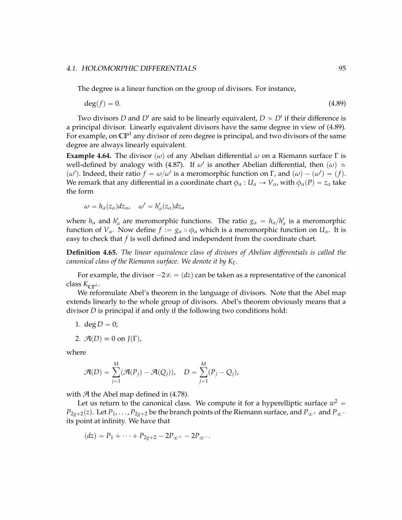
4.1. HOLOMORPHIC DIFFERENTIALS 95
The degree is a linear function on the group of divisors. For instance,
degp f q “ 0. (4.89)
Two divisors D and D1 are said to be linearly equivalent, D » D1 if their difference isa principal divisor. Linearly equivalent divisors have the same degree in view of (4.89).For example, on CP1 any divisor of zero degree is principal, and two divisors of the samedegree are always linearly equivalent.Example 4.64. The divisor pωq of any Abelian differential ω on a Riemann surface Γ iswell-defined by analogy with (4.87). If ω1 is another Abelian differential, then pωq »pω1q. Indeed, their ratio f “ ωω1 is a meromorphic function on Γ, and pωq ´ pω1q “ p f q.We remark that any differential in a coordinate chart φα : Uα Ñ Vα, with φαpPq “ zα takethe form
ω “ hαpzαqdzα, ω1 “ h1αpzαqdzα
where hα and h1α are meromorphic functions. The ratio gα “ hαh1α is a meromorphicfunction of Vα. Now define f :“ gα ˝ φα which is a meromorphic function on Uα. It iseasy to check that f is well defined and independent from the coordinate chart.
Definition 4.65. The linear equivalence class of divisors of Abelian differentials is called thecanonical class of the Riemann surface. We denote it by KΓ.
For example, the divisor ´28 “ pdzq can be taken as a representative of the canonicalclass KCP1 .
We reformulate Abel’s theorem in the language of divisors. Note that the Abel mapextends linearly to the whole group of divisors. Abel’s theorem obviously means that adivisor D is principal if and only if the following two conditions hold:
1. deg D “ 0;
2. ApDq ” 0 on JpΓq,
where
ApDq “Mÿ
j“1
pApP jq ´ApQ jqq, D “
Mÿ
j“1
pP j ´Q jq,
withA the Abel map defined in (4.78).Let us return to the canonical class. We compute it for a hyperelliptic surface w2 “
P2g`2pzq. Let P1, . . . ,P2g`2 be the branch points of the Riemann surface, and P8` and P8´its point at infinity. We have that
pdzq “ P1 ` ¨ ¨ ¨ ` P2g`2 ´ 2P8` ´ 2P8´ .
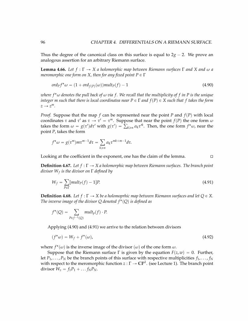
96 CHAPTER 4. DIFFERENTIALS ON A RIEMANN SURFACE.
Thus the degree of the canonical class on this surface is equal to 2g ´ 2. We prove ananalogous assertion for an arbitrary Riemann surface.
Lemma 4.66. Let f : Γ Ñ X a holomorphic map between Riemann surfaces Γ and X and ω ameromorphic one form on X, then for any fixed point P P Γ
ordP f ˚ω “ p1` ord f pPqpωqqmultPp f q ´ 1 (4.90)
where f ˚ω denotes the pull back of ω via f . We recall that the multiplicity of f in P is the uniqueinteger m such that there is local coordinatea near P P Γ and f pPq P X such that f takes the formz Ñ zm.
Proof. Suppose that the map f can be represented near the point P and f pPq with localcoordinates τ and τ1 as τ Ñ τ1 “ τm. Suppose that near the point f pPq the one form ωtakes the form ω “ gpτ1qdτ1 with gpτ1q “
ř
kěn αkτ1k. Then, the one form f ˚ω, near the
point P, takes the form
f ˚ω “ gpτmqmτm´1dτ “ÿ
kěn
αkτmk`m´1dτ.
Looking at the coefficient in the exponent, one has the claim of the lemma.
Definition 4.67. Let f : Γ Ñ X a holomorphic map between Riemann surfaces. The branch pointdivisor W f is the divisor on Γ defined by
W f “ÿ
PPΓ
rmultPp f q ´ 1sP. (4.91)
Definition 4.68. Let f : Γ Ñ X be a holomoprhic map between Riemann surfaces and let Q P X.The inverse image of the divisor Q denoted f ˚pQq is defined as
f ˚pQq “ÿ
PP f´1pQq
multpp f q ¨ P.
Applying (4.90) and (4.91) we arrive to the relation between divisors
p f ˚ωq “ W f ` f ˚pωq, (4.92)
where f ˚pωq is the inverse image of the divisor pωq of the one form ω.Suppose that the Riemann surface Γ is given by the equation Fpz,wq “ 0. Further,
let P1, . . . ,PN be the branch points of this surface with respective multiplicities f1, . . . , fNwith respect to the meromorphic function z : Γ Ñ CP1. (see Lecture 1). The branch pointdivisor Wz “ f1P1 ` . . . fNPN.
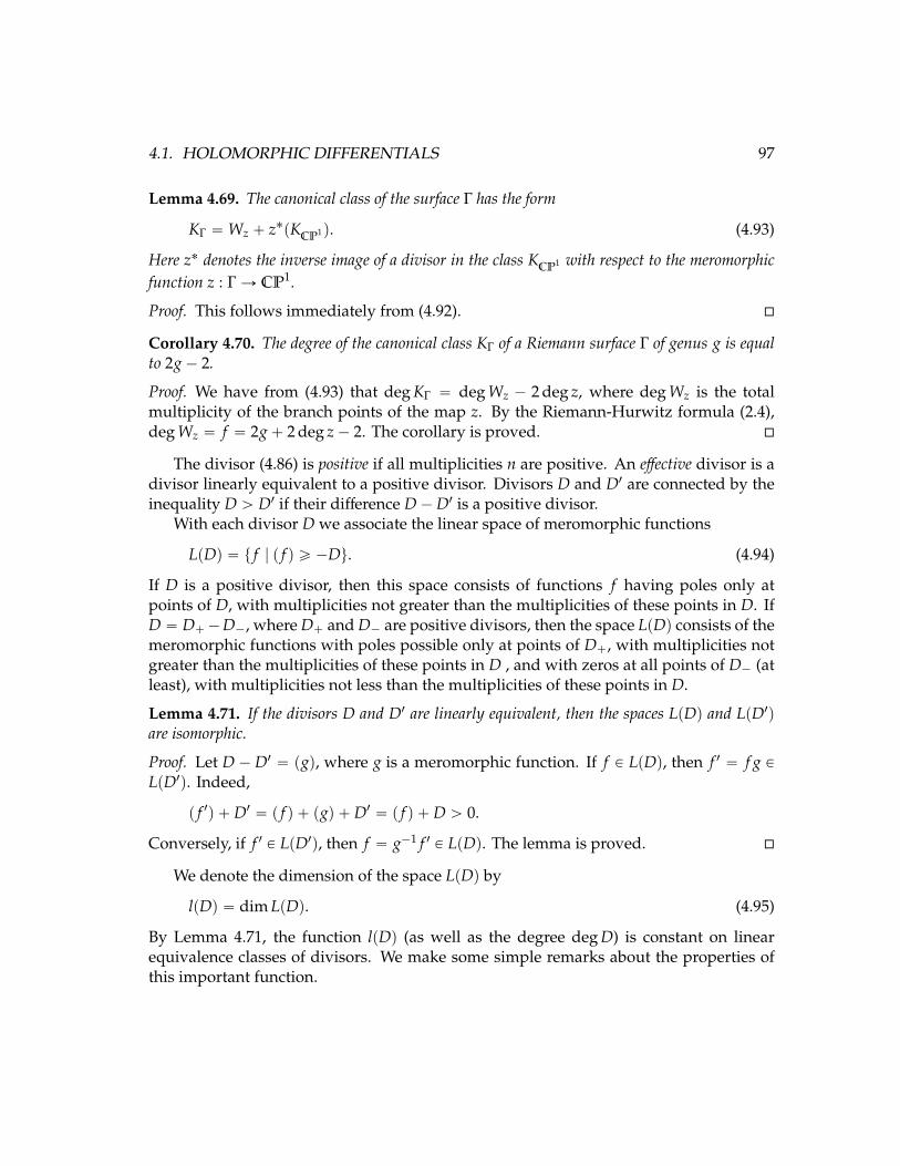
4.1. HOLOMORPHIC DIFFERENTIALS 97
Lemma 4.69. The canonical class of the surface Γ has the form
KΓ “ Wz ` z˚pKCP1q. (4.93)
Here z˚ denotes the inverse image of a divisor in the class KCP1 with respect to the meromorphicfunction z : Γ Ñ CP1.
Proof. This follows immediately from (4.92).
Corollary 4.70. The degree of the canonical class KΓ of a Riemann surface Γ of genus g is equalto 2g´ 2.
Proof. We have from (4.93) that deg KΓ “ deg Wz ´ 2 deg z, where deg Wz is the totalmultiplicity of the branch points of the map z. By the Riemann-Hurwitz formula (2.4),deg Wz “ f “ 2g` 2 deg z´ 2. The corollary is proved.
The divisor (4.86) is positive if all multiplicities n are positive. An effective divisor is adivisor linearly equivalent to a positive divisor. Divisors D and D1 are connected by theinequality D ą D1 if their difference D´D1 is a positive divisor.
With each divisor D we associate the linear space of meromorphic functions
LpDq “ t f | p f q ě ´Du. (4.94)
If D is a positive divisor, then this space consists of functions f having poles only atpoints of D, with multiplicities not greater than the multiplicities of these points in D. IfD “ D`´D´, where D` and D´ are positive divisors, then the space LpDq consists of themeromorphic functions with poles possible only at points of D`, with multiplicities notgreater than the multiplicities of these points in D , and with zeros at all points of D´ (atleast), with multiplicities not less than the multiplicities of these points in D.
Lemma 4.71. If the divisors D and D1 are linearly equivalent, then the spaces LpDq and LpD1qare isomorphic.
Proof. Let D ´ D1 “ pgq, where g is a meromorphic function. If f P LpDq, then f 1 “ f g PLpD1q. Indeed,
p f 1q `D1 “ p f q ` pgq `D1 “ p f q `D ą 0.
Conversely, if f 1 P LpD1q, then f “ g´1 f 1 P LpDq. The lemma is proved.
We denote the dimension of the space LpDq by
lpDq “ dim LpDq. (4.95)
By Lemma 4.71, the function lpDq (as well as the degree deg D) is constant on linearequivalence classes of divisors. We make some simple remarks about the properties ofthis important function.
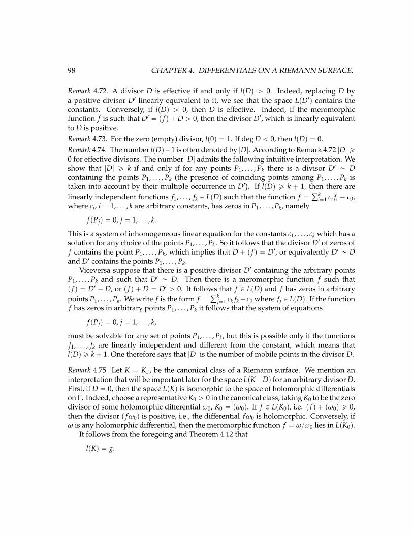
98 CHAPTER 4. DIFFERENTIALS ON A RIEMANN SURFACE.
Remark 4.72. A divisor D is effective if and only if lpDq ą 0. Indeed, replacing D bya positive divisor D1 linearly equivalent to it, we see that the space LpD1q contains theconstants. Conversely, if lpDq ą 0, then D is effective. Indeed, if the meromorphicfunction f is such that D1 “ p f q `D ą 0, then the divisor D1, which is linearly equivalentto D is positive.Remark 4.73. For the zero (empty) divisor, lp0q “ 1. If deg D ă 0, then lpDq “ 0.Remark 4.74. The number lpDq´1 is often denoted by |D|. According to Remark 4.72 |D| ě0 for effective divisors. The number |D| admits the following intuitive interpretation. Weshow that |D| ě k if and only if for any points P1, . . . ,Pk there is a divisor D1 » Dcontaining the points P1, . . . ,Pk (the presence of coinciding points among P1, . . . ,Pk istaken into account by their multiple occurrence in D1). If lpDq ě k ` 1, then there arelinearly independent functions f1, . . . , fk P LpDq such that the function f “
řki“1 ci fi ´ c0,
where ci, i “ 1, . . . , k are arbitrary constants, has zeros in P1, . . . ,Pk, namely
f pP jq “ 0, j “ 1, . . . , k.
This is a system of inhomogeneous linear equation for the constants c1, . . . , ck which has asolution for any choice of the points P1, . . . ,Pk. So it follows that the divisor D1 of zeros off contains the point P1, . . . ,Pk, which implies that D ` p f q “ D1, or equivalently D1 » Dand D1 contains the points P1, . . . ,Pk.
Viceversa suppose that there is a positive divisor D1 containing the arbitrary pointsP1, . . . ,Pk and such that D1 » D. Then there is a meromorphic function f such thatp f q “ D1 ´ D, or p f q ` D “ D1 ą 0. It follows that f P LpDq and f has zeros in arbitrarypoints P1, . . . ,Pk. We write f is the form f “
řkj“1 ck fk´ c0 where f j P LpDq. If the function
f has zeros in arbitrary points P1, . . . ,Pk it follows that the system of equations
f pP jq “ 0, j “ 1, . . . , k,
must be solvable for any set of points P1, . . . ,Pk, but this is possible only if the functionsf1, . . . , fk are linearly independent and different from the constant, which means thatlpDq ě k` 1. One therefore says that |D| is the number of mobile points in the divisor D.
Remark 4.75. Let K “ KΓ, be the canonical class of a Riemann surface. We mention aninterpretation that will be important later for the space LpK´Dq for an arbitrary divisor D.First, if D “ 0, then the space LpKq is isomorphic to the space of holomorphic differentialson Γ. Indeed, choose a representative K0 ą 0 in the canonical class, taking K0 to be the zerodivisor of some holomorphic differential ω0, K0 “ pω0q. If f P LpK0q, i.e. p f q ` pω0q ě 0,then the divisor p fω0q is positive, i.e., the differential fω0 is holomorphic. Conversely, ifω is any holomorphic differential, then the meromorphic function f “ ωω0 lies in LpK0q.
It follows from the foregoing and Theorem 4.12 that
lpKq “ g.
4.1. HOLOMORPHIC DIFFERENTIALS 99
Lemma 4.76. For a positive divisor D the space LpK ´Dq is isomorphic to the space
ΩpDq “ tω P H1pΓq | pωq ´D ě 0u
Proof. We choose a representative K0 ą 0 in the canonical class, taking K0 to be thezero divisor of some holomorphic differential ω0, K0 “ pω0q. If f P LpK0 ´ Dq, thenthe differential fω0 is holomorphic and has zeros at the points of D, i.e., fω0 P ΩpDq.Conversely, if ω P ΩpDq, then f “ ωω0 P LpK0 ´Dq. The assertion is proved.
The main way of getting information about the numbers lpDq is the Riemann-RochTheorem.
Theorem 4.77 (Riemann Roch Theorem). For any divisor D
lpDq “ 1` deg D´ g` lpK ´Dq. (4.96)
Proof. For surfaces Γ of genus 0 (which are isomorphic to CP1 in view of Problem 6.1)the Riemann-Roch theorem is a simple assertion about rational functions (verify!). ByRemarks 4.73 and 4.75 (above) the Riemann-Roch theorem is valid for D “ H.
We first prove (4.96) for positive divisors D ą 0. Let D “řm
k“1 nkPk where all thenk ą 0. We first verify the arguments when all the nk are“ 1, i.e., m “ deg D. Let f P LpDqbe a nonconstant function.
We consider the Abelian differential ω “ d f . It has double poles and zero residues atthe points P1, . . . ,Pm and does not have other singularities. Therefore, it is representablein the form
Ω “ d f “mÿ
k`1
ckΩp1qPk` ψ
where Ωp1qPk
are normalized differentials of the second kind (see Lecture 4.1.3), c1, . . . , cm
are constants, and the differential ψ is holomorphic. Since the function f pPq “şP
P0Ω is
single-valued on Γ, the integralşP
P0Ωis independent from the path of integration. This
implies that¿
αi
Ω “ 0,¿
bi
Ω “ 0, i “ 1, . . . , g. (4.97)
From the vanishing of the α-periods of the meromorphic differentials Ωp1qPk
we get thatψ “ 0 (see Corollary 4.17). From the vanishing of the β-period we get, by (4.30) withn “ 1, that
0 “¿
βi
Ω “
mÿ
k“1
ckψikpzkq|zk“0, i “ 1, . . . , g, (4.98)
100 CHAPTER 4. DIFFERENTIALS ON A RIEMANN SURFACE.
where zk is a local parameter in a neighborhood of Pk, zkpPkq “ 0, k “ 1, . . . ,m, andthe basis of holomorphic differentials are written in a neighborhood of Pk in the formωi “ ψikpzqdzk. Defining ωipPkq :“ ψikp0q, we write the system (4.98) in the form
¨
˚
˚
˝
ω1pP1q ω1pP2q . . . ω1pPmq
ω2pP1q ω2pP2q . . . ω2pPmq
. . . . . . . . . . . .ωgpP1q ωgpP2q . . . ωgpPmq
˛
‹
‹
‚
¨
˚
˚
˝
c1c2. . .cm
˛
‹
‹
‚
“ 0, (4.99)
We have obtained a homogeneous linear system of m “ deg D equations in the coefficientsc1, . . . , cm. The nonzero solutions of this systems are in a one-to-one correspondence withthe nonconstant functions f in LpDq, where f can be reproduced from a solution c1, . . . , cmof the system (4.98) in the form
f pPq “mÿ
k“1
ck
ż P
P0
Ωp1qPk.
Thus lpDq “ 1 ` deg D ´ rankA where A is the matrix of holomorphic differentials in(4.99) (the 1 is added because the constant function belong to the space LpDq). On theother hand the rank of the matrixA has another interpretation. Consider the holomorphicdifferential ω “
řgj“1 a jω j. Such differential ω belongs to the space ΩpDq if
ωpPkq “ 0, k “ 1, . . . ,m.
The above system of equations can be written in the equivalent form
`
a1 a2 . . . ag˘
¨
˝
ω1pP1q . . . ω1pPmq
. . . . . . . . .ωgpP1q . . . ωgpPmq
˛
‚“ 0. (4.100)
The number of solutions of this system is equal to g´ rankA and it is in one to one cor-respondence with the linearly independent holomorphic differentials in ΩpDq. ThereforedimΩpDq “ g´ rankA. On the other hand we have obtained that
lpDq “ 1` deg D´ rankA
so that combining the two equations we obtain
lpDq “ 1` deg D´ g` dimΩpDq “ 1` deg D´ g` lpK ´Dq
where the second identity is due to the fact that the space ΩpDq and LpK´Dq are isomorphicfor positive divisors. Accordingly the Riemann-Roch theorem has been proved in thiscase.
4.1. HOLOMORPHIC DIFFERENTIALS 101
We explain what happens when the positive divisor D has multiple points. Forexample suppose that D “ n1P1 ` . . . . Then ω “ d f “
řn1j“1 c j
1Ωp jqP1` . . . and the system
(4.98) can be written in the form
n1ÿ
j“1
c j1
1j!
d j´1ψi1
dz j´11
ˇ
ˇ
ˇ
ˇ
ˇ
ˇ
z1“0
` ¨ ¨ ¨ “ 0
If the rank of the coefficient matrix of this system is denoted (as above) by rankA, thedimension of the space LpDq is equal to lpDq “ 1`deg D´ rankAwhile the dimension ofthe space ΩpDq is equal to g´ rankA. We have proved the Riemann-Roch theorem for allpositive divisors and hence for all effective divisors, which (accordingly to Remark 4.72)are distinguished by the condition lpDq ą 0. Next we note that the relation in this theoremcan be written in the form
lpDq ´12
deg D “ lpK ´Dq ´12
degpK ´Dq, (4.101)
which is symmetric with respect to the substitution D Ñ K ´ D. Therefore the theoremis proved for all divisors D such that D or K ´ D is equivalent to an integral divisor. Ifneither D nor K ´D are equivalent to an integral divisor, then lpDq “ 0 and lpK ´Dq “ 0and the Riemann-Roch theorem reduces in this case to the equality
deg D “ g´ 1. (4.102)
Let us prove this equality. We represent D in the form D “ D` ´D´, where D` and D´are positive divisors and deg D´ ą 0. It follows from the validity of the Riemann-Rochtheorem for D` that lpD`q ě deg D` ´ g ` 1 “ deg D ` deg D´ ´ g ` 1. Therefore ifdeg D ě g, then lpD`q ě 1` deg D´. Then the space LpD`q contains a nonzero functionvanishing on D´, i.e. belonging to the space LpD` ´ D´q “ LpDq. This contradicts thecondition lpDq “ 0. Similarly, the assumption degpK ´ Dq ď g leads to a contradiction.This implies (4.102). The theorem is proved.
4.1.6 Some consequences of the Riemann-Roch theorem. The structure ofsurfaces of genus 1. Weierstrass points. The canonical embedding
Corollary 4.78. If deg D ě g, then the divisor D is effective.
Corollary 4.79. The Riemann inequality
lpDq ě 1` deg D´ g, (4.103)
holds for deg D ě g.
102 CHAPTER 4. DIFFERENTIALS ON A RIEMANN SURFACE.
Definition 4.80. A positive divisor D is called special if
dimΩpDq ą 0.
We remark that any effective divisor of degree less then g is special since lpDq ą 0 andby Riemann-Roch theorem this implies dimΩpDq ą 0.
Corollary 4.81. If deg D ą 2g´ 2, then D is nonspecial.
Proof. For deg D ą 2g ´ 2 we have that degpK ´ Dq ă 0, hence lpK ´ Dq “ 0 (seeRemark 4.73). The corollary is proved.
Exercise 4.82: Suppose that k ě g; let the Abel mapping A : Γ Ñ JpΓq (see Lecture 4.1.4)be extended to the kth-power mapping
Ak : Γˆ ¨ ¨ ¨ ˆ Γlooooomooooon
k times
Ñ JpΓq
by setting AkpP1, . . . ,Pkq “ ApP1q`¨ ¨ ¨`ApPkq (it can actually be assumed that Ak maps intoJpΓq the kth symmetric power SkΓ, whose points are the unordered collections pP1, . . . ,Pkq
of points of Γ). Prove that the special divisors of degree k are precisely the critical pointsof the Abel mapping Ak. Deduce from this that a divisor D with deg D ě g in generalposition is nonspecial.
Remark 4.83. Let deg D “ 0, then if D is equivalent to a divisor of a meromorphic function,then LpDq “ 1 otherwise LpDq “ 0. Let deg D “ 2g ´ 2, then if D is equivalent to thecanonical divisor, then lpDq “ g otherwise lpDq “ g ´ 1. Furthermore if deg D ą 2g ´ 2,then by Riemann Roch theorem one has lpDq “ 1 ` deg D ´ g. If 0 ď deg D ď g ´ 1 theminimum value of lpDq is zero while for g ď deg D ď 2g´ 2, minplpDqq “ 1´ g` deg D.
The values of lpDq for 0 ď deg D ď 2g´ 2 are estimated by the Clifford theorem.
Theorem 4.84. If 0 ď deg D ď 2g´ 2, then
lpDq ď 1`12
deg D. (4.104)
Proof. If lpDq “ 0 or lpK ´ Dq “ 0, the proof of the theorem is straightforward. Let usassume that lpDq ą 0 and lpK ´ Dq ą 0 and consider the map LppDq ˆ LpK ´ Dq Ñ LpKqgiven by p f , hq Ñ f h where p f , hq P LppDqˆLpK´Dq. Let V be the subspace in LpKqwhichis the image of this map. Then one has
g “ lpKq ě dim V “ lpDqlpK ´Dq ě lpDq ` lpK ´Dq ´ 1
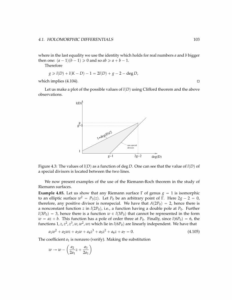
4.1. HOLOMORPHIC DIFFERENTIALS 103
where in the last equality we use the identity which holds for real numbers a and b biggerthen one: pa´ 1qpb´ 1q ě 0 and so ab ě a` b´ 1.
Therefore
g ě lpDq ` lpK ´Dq ´ 1 “ 2lpDq ` g´ 2´ deg D,
which implies (4.104).
Let us make a plot of the possible values of lpDq using Clifford theorem and the aboveobservations.
g−1 2g−2
g−1
1
g
deg(D)
l(D)
1+deg(D)/2
non special
divisors
Figure 4.3: The values of lpDq as a function of deg D. One can see that the value of lpDq ofa special divisors is located between the two lines.
We now present examples of the use of the Riemann-Roch theorem in the study ofRiemann surfaces.Example 4.85. Let us show that any Riemann surface Γ of genus g “ 1 is isomorphicto an elliptic surface w2 “ P3pzq. Let P0 be an arbitrary point of Γ. Here 2g ´ 2 “ 0,therefore, any positive divisor is nonspecial. We have that Ap2P0q “ 2, hence there isa nonconstant function z in lp2P0q, i.e., a function having a double pole at P0. Furtherlp3P0q “ 3, hence there is a function w P lp3P0q that cannot be represented in the formw “ az ` b. This function has a pole of order three at P0. Finally, since lp6P0q “ 6, thefunctions 1, z, z2, z3,w,w2,wz which lie in lp6P0q are linearly independent. We have that
a1w2 ` a2wz` a3w` a4z3 ` a5z2 ` a6z` a7 “ 0. (4.105)
The coefficient a1 is nonzero (verify). Making the substitution
w Ñ w´ˆ
a2
2a1z`
a3
2a1
˙
104 CHAPTER 4. DIFFERENTIALS ON A RIEMANN SURFACE.
we get the equation of an elliptic curve from (4.105).
Example 4.86 (Riemann count of the moduli space of Riemann surface). Consider aRiemann surface Γ of genus g and a meromorphic function of degree n ą g. Suchfunction represents Γ as a n-sheeted covering of the complex plane, branched over anumber of points with total branching number b f equal to
b f “ 2n` 2g´ 2
where the Riemann-Hurwitz formula has been used. Generically the branch pointshave branching number equal to one so that b f is also equal to the branch points of theRiemann surface. From the Riemann existence theorem, given the branch points and apermutation associated to each branch point such that the corresponding monodromygroup is a transitive sub-group of Sn, then one can construct a Riemann surface Γ. Letf : Γ Ñ P1 be the obvious projection map. Such map To any set of branch points itcorrespond a finite number of Riemann surface of genus g together with a meromorphicfunction of degree n. Riemann surface is determined uniquely up to isomorphism.
Any meromorphic function of degree n on Γ will represent Γ as a n-sheeted coveringof the complex plane. Let D8 be the divisor of poles of f . Since the degree of f is equalto n then deg D8 “ n. Furthermore from Riemann-Roch theorem
lpD8q “ n` 1´ g.
So the freedom of choosing the function f is given by the position of the poles, and thisgives n parameters, and the number of functions having poles in D8, which is equal ton`1´g. The total number of parameters in choosing the meromorphic function of degreen is 2n´ 1´ g. So the total number of parameters for describing a curve of genus g is
2n` 2g´ 2´ p2n´ 1´ gq “ 3g´ 3.
Definition 4.87 (Weierstrass points). A point P0 of a Riemann surface Γ of genus g is called aWeierstrass point if lpkP0q ą 1 for some k ď g.
It is clear that in the definition of a Weierstrass point it suffices to require that lpgP0q ą 1when g ě 2. There are no Weierstrass points on a surface of genus g “ 1. On hyperellipticRiemann surfaces of genus g ą 1 all branch points are Weierstrass points, since there existfunctions with second-order poles at the branch points (see Lecture 3).
Definition 4.88. A Riemann surface is called hyperelliptic if and only if it admits a non constantmeromorphic function of degree 2.
The use of Weierstrass points can be illustrated in the next exercise.
4.1. HOLOMORPHIC DIFFERENTIALS 105
Exercise 4.89: Let Γ be a Riemann surface of genus g ą 1, and P0 a Weierstrass point of it,with lp2P0q ą 1. Prove that Γ is hyperelliptic. Prove that the surface is also hyperellipticif lpP`Qq ą 1 for two points P and Q.
Exercise 4.90: Let Γ be a hyperellitpic Rieamnn surface and z a function of degree two.Prove that any other function f of degree two is a Moebius transformation of z.
We show that there exist Weierstrass points on any Riemann surface Γ of genus g ą 1.
Lemma 4.91. Suppose that z is a local parameter in a neighborhood P0, zpP0q “ 0; assume thatlocally the basis of holomorphic differentials has the form ωi “ ψipzqdz, i “ 1, . . . , g. Consider thedeterminant
Wpzq “ det
¨
˚
˝
ψ1pzq ψ11pzq . . . ψpg´1q1 pzq
. . . . . . . . .
ψgpzq ψ1gpzq . . . ψpg´1qg pzq
˛
‹
‚. (4.106)
The point P0 is a Weierstrass point if and only if Wp0q “ 0.
Proof. If P0 is a Weierstrass point, i.e., lpgP0q ą 1, then lpK´gP0q ą 0 by the Riemann-Rochtheorem. Hence, there is a holomorphic differential with a g-fold zero at P0 on Γ. Thecondition that there be such a differential can be written in the form Wp0q “ 0 (cf. theproof of the Riemann-Roch theorem). The lemma is proved.
Lemma 4.92. Under a local change of parameter z “ zpwq the quantity W transforms according
to the rule Wpwq “ˆ
dzdw
˙12 gpg`1q
Wpzq.
Proof. Suppose that ωi “ ψipzqdz “ ψipwqdw. Then each ψi “ ψidzdw
, i “ 1, . . . , g. This
implies that the derivatives dkψidwk can be expressed for each i in terms of the derivativesdlψidzl by means of a triangular transformation of the form
dkψi
dwk“
ˆ
dzdw
˙k`1 dkψi
dzk`
k´1ÿ
j“1
c jd jψi
dz j , i “ 1, . . . g
(the coefficients cs in this formula are certain differential polynomials in zpwq). Thestatement of the Lemma readily follows from the transformation rule.
Let us define the weight of a Weierstrass point P0 as the multiplicity of zero of Wpzq atthis point. According to the previous Lemma the definition of weight does not dependon the choice of the local parameter.
The proof of existence of Weierstrass points for g ą 1 can be easily obtained from thefollowing statement.
106 CHAPTER 4. DIFFERENTIALS ON A RIEMANN SURFACE.
Lemma 4.93. The total weight of all Weierstrass points on the Riemann surface Γ of genus g isequal to pg´ 1q g pg` 1q.
Proof. Let us consider the ratioWpzqψN
1 pzq.
Here N “ 12 gpg` 1q. According to lemma (4.92), the above ratio does not depend on the
choice of the local parameter and, hence, it is a meromorphic function on Γ. This functionhas poles of multiplicity N at the zeroes of the differentialω1 (the total number of all polesis equal to 2g´ 2). Therefore this function must have N p2g´ 2q “ pg´ 1q g pg` 1q zeroes(as usual, counted with their multiplicities). These zeroes are the Weierstrass points.
Let us do few more remarks about the Weierstrass points. Given a point P0 P Γ, let usconsider the dimension lpk P0q as a function of the integer argument k. This function hasthe following properties. According to figure (4.3) we have
1 ď lpk P0q ď g, 1 ď k ď 2g´ 1.
In particular l pp2g´ 1qP0q “ g. It follows that while k increases 2g´ 2 times the functionlpk P0q increases only g ´ 1 times. The next lemma shows that the function lpk P0q is apiece-wise constant function where each step has size equal to one.
Lemma 4.94.
lpk P0q “
"
l ppk´ 1qP0q ` 1, if there exists a function with a pole of order k at P0l ppk´ 1qP0q , if such a function does not exist
Proof. The space Lpk P0q is larger then the space Lppk´1qP0q therefore lpk P0q ě lppk´1qP0q.On the other hand, dimΩpkP0q ď dimΩppk´ 1qP0q. From the Riemann Roch theorem onehas
lpk P0q ´ lppk´ 1qP0q “ 1` dimΩpkP0q ´ dimΩppk´ 1qP0q
which, when combined with the above two inequalities, gives the statement.
When lpk P0q “ lppk´1qP0qwe will say that the number k is a gap at the point P0. Fromthe previous remarks it follows the following Weierstrass gap theorem:
Theorem 4.95. There are exactly g gaps 1 “ a1 ă ... ă ag ă 2g at any point P0 of a Riemannsurface of genus g.
The gaps have the form ai “ i, i “ 1, . . . , g, for a point P0 in general position (whichis not a Weierstrass point). Namely for a non Weierstrass point the function lpkP0q is nonzero only for k ą g and one has lpkP0q “ 1 ` k ´ g for k ą g. A Weierstrass point P0 is
4.1. HOLOMORPHIC DIFFERENTIALS 107
called normal if the Weierstrass gap sequence takes the form 1, 2, . . . , g´ 1, g` 1 where gis the genus of the surface. Namely a meromorphic function with only a pole in P0 hasorder at least equal to g. Normal Weierstrass points are generic. A Weierstrass point P0 iscalled hyperelliptical is the Weierstrass gap sequence takes the form 1, 3, 5, . . . , 2g´ 1. Inthis case a meromorphic function with only a pole in P0 has order equal to two.
Exercise 4.96: Show that every compact Riemann surface of genus g is conformallyequivalent to a pg` 1q´sheeted covering surface of the complex plane.
Exercise 4.97: Prove that for branch points of a hyperelliptic Riemann surface of genus gthe gaps have the form ai “ 2i´ 1, i “ 1, . . . , g. Prove that a hyperelliptic surface does nothave other Weierstrass points. Next suppose that the hyperelliptic Riemann surface hasgenus 2 and let P0 be a Weierstrass point. Show that there exist meromorphic functions zand w with only a pole in P0 and such that
w2 ` a1wz` a2wz2 ` a3z5 ` a4z4 ` a5z3 ` a6z2 ` a7z` a8 “ 0.
Exercise 4.98: Prove that any Riemann surface of genus 2 is hyperelliptic.
Exercise 4.99: Let Γ be a hyperelliptic Riemann surface of the form w2 “ P2g`lpzq.Prove that any birational (biholomorphic) automorphism Γ Ñ Γ has the form pz,wq Ñ
paz` bcz` d
,˘wq, where the linear fractional transformation leaves the collection of zeros of
P2g`2pzq invariant.
Example 4.100 (The canonical embedding). . Let Γ be an arbitrary Riemann surface ofgenus g ě 2. We fix on Γ a canonical basis of cycles a1, . . . , ag, b1, . . . , bg; let ω1, . . . , ωg bethe corresponding normal basis of holomorphic differentials. This basis gives a canonicalmapping Γ Ñ CPg´1 according to the rule
P Ñ pω1pPq : ω2pPq : ¨ ¨ ¨ : ωgpPqq. (4.107)
Indeed, it suffices to see that all the differentials ω1, . . . , ωg cannot simultaneously vanishat some point of the surface. If P were a point at which any holomorphic differentialvanished, i.e., lpK ´ Pq “ g, (see Remark 4.75), then lpPq would be “ 2 in view of theRiemann-Roch theorem, and this means that the surface Γ is rational (verify!). Accordingly(4.107) really is a mapping Γ Ñ CPg´1; it is obviously well-defined.
Lemma 4.101. If Γ is a nonhyperelliptic surface of genus g ě 3, then the canonical mapping(4.107) is a smooth embedding. If Γ is a hyperelliptic surface of genus g ě 2, then the image of thecanonical embedding is a rational curve, and the mapping itself is a two-sheeted covering.
108 CHAPTER 4. DIFFERENTIALS ON A RIEMANN SURFACE.
Proof. We prove that the mapping (4.107) is an embedding. Assume not: assume that thepoints P1 and P2 are merged into a single point by this mapping. This means that therank of the matrix
¨
˝
ω1pP1q ω1pP2q
. . . . . .ωgpP1q ωgpP2q
˛
‚
is equal to 1. But then lpP1`P2q ą 1 (see the proof of the Riemann-Roch theorem). Hence,there exists on Γ a nonconstant function with two simple poles at P1 and P2 i.e., the surfaceΓ is hyperelliptic. The smoothness is proved similarly: if it fails to hold at a point P, thenthe rank of the matrix
¨
˝
ω1pPq ω11pPq. . . . . .ωgpPq ω1gpPq
˛
‚
is equal to 1. Then lp2Pq ą 1, and the surface is hyperelliptic. Finally, suppose that Γ ishyperelliptic. Then it can be assumed of the form w2 “ P2g`1pzq. Its canonical mappingis determined by the differentials (5.42). Performing a projective transformation of thespace CPg´1 with the matrix pc jkq (see the formula (5.42)), we get the following form forthe canonical mapping:
P “ pz,wq Ñ p1 : z : ¨ ¨ ¨ : zg´1q (4.108)
Its properties are just as indicated in the statement of the lemma. The lemma is proved.
We remark that the canonical mapping smoothly embeds a nonhyperelliptic Riemannsurface of genus g in Pg´1. It is proved in [16] that the image of such embedding canbe smoothly project to P3. Namely every smooth Riemann surface has an holomorphicembedding in P3.
Exercise 4.102: Suppose that the Riemann surface Γ is given in CP2 by the equationÿ
i` j“4
ai jξiη jζ4´i´ j “ 0, (4.109)
and this curve is nonsingular in CP2 (construct an example of such a nonsingular curve).Prove that the genus of this surface is equal to 3 and the canonical mapping is the identityup to a projective transformation of CP2. Prove that Γ is a non hyperelliptic surface.Prove that any non hyperelliptic surface of genus 3 can be obtained in this way.
The range Γ1 Ă CPg´1 of the canonical mapping is called the canonical curve.
Exercise 4.103: Prove that any hyperplane in CPg´1 intersects the canonical curve Γ1 in2g´ 2 points (counting multiplicity).
Chapter 5
Jacobi inversion problem andtheta-functions
5.1 Statement of the Jacobi inversion problem. Definition andsimplest properties of general theta functions
In Lecture 4.1.2 we saw that inversion of an elliptic integral leads to elliptic functions. Fora surface of genus g ą 1 the Inversion of integrals of Abelian differentials is not possiblesince any such differential has zeros (at least 2g ´ 2zeros). Instead of the problem ofinverting a single Abelian integral, Jacobi proposed for hyperelliptic surfaces w2 “ P5pzqthe problem of solving the system
P1ż
P0
dza
P5pzq`
P2ż
P0
dza
P5pzq“ η1
P1ż
P0
zdza
P5pzq`
P2ż
P0
zdza
P5pzq“ η2
(5.1)
where η1, η2 are given numbers from which the location of the points P1 “ pz1,w1q,P2 “ pz2,w2q is to be determined. It is clear, moreover, that P1 and P2 are determined from(5.1) only up to permutation. Jacobi’s idea was to express the symmetric functions of P1and P2 as functions of η1 and η2. He noted also that this will give meromorphic functionsof η1 and η2 whose period lattice is generated by the periods of the basis of holomorphicdifferentials dz
a
P5pzq and zdza
P5pzq. This Jacobi inversion problem was solved byGoepel and Rosenhain by means of the apparatus of theta functions of two variables.The generalization of the Jacobi inversion problem to arbitrary Riemann surfaces and
109
110 CHAPTER 5. JACOBI INVERSION PROBLEM AND THETA-FUNCTIONS
its solution are due to Riemann. We give a precise statement of the Jacobi inversionproblem. Let Γ be an arbitrary Riemann surface of genus g, and fix a canonical basis ofcycles α1, . . . , αg, β1, . . . , βg on Γ; as above let ω1, . . . , ωg be be the corresponding basis ofnormalized holomorphic differentials. Recall (see Lecture 4.1.4) that the Abel mappinghas the form
A : Γ Ñ JpΓq, ApPq “ pu1pPq, . . . ,ugpPqq, (5.2)
where JpΓq is the Jacobi variety,
uipPq “
Pż
P0
ωi, (5.3)
P0 is a particular point of Γ, and the path of integration from P0 to P is the same forall i “ 1, . . . , g. Consider the gth symmetric power SgΓ of Γ. The unordered collectionspP1, . . . ,Pgq of g points of Γ are the points of the manifold SgΓ. The meromorphic functionson SgΓ are the meromorphic symmetric functions of g variables P1, . . . ,Pg, P j P Γ. TheAbel mapping (5.2) determines a mapping
Apgq : SgΓ Ñ JpΓq, AgpP1, . . . ,Pgq “ ApP1q ` ¨ ¨ ¨ ` ApPgq, (5.4)
which we also call the Abel mapping.
Lemma 5.1. If the divisor D “ P1 ` ¨ ¨ ¨ ` Pg is nonspecial, then in a neighborhood of a pointApgqpP1, ...,Pgq P JpΓq the mapping Apgq has a single-valued inverse.
Proof. Suppose that all the points are distinct; let z1, . . . , zg be local parameters in neigh-borhoods of the respective points P1, . . . ,Pg with zkpPkq “ 0 and ωi “ ψikpzkqdzk thenormalized holomorphic differentials in a neighborhood of Pk. The Jacobi matrix of themapping (5.4) has the following form at the points pP1, . . . ,Pgq
¨
˝
ψ11pz1 “ 0q . . . ψ1gpzg “ 0q. . . . . . . . .
ψg1pz1 “ 0q . . . ψggpzg “ 0q
˛
‚.
If the rank of this matrix is less than g, then lpK ´ Dq ą 0, i.e., the divisor D is specialby the Riemann-Roch theorem. The case when not all the points P1, . . . ,Pg are distinct istreated similarly. We now prove that the inverse mapping is single-valued. Assume thatthe collection of points pP11, . . . ,P
1gq is also carried into ApgqpP1, . . . ,Pgq. Then the divisor
D1 “ P11 ` ¨ ¨ ¨ ` P1g is linearly equivalent to D by Abel’s theorem. If D1 , D, then therewould be a meromorphic function with poles at points of D and with zeros at points ofD1. This would contradict the fact that D is nonspecial. Hence, D1 “ D, and the pointsP11, . . . ,P
1g differ from P1, . . . ,Pg only in order. The lemma is proved.
5.2. THETA-FUNCTIONS 111
Since a divisor P1 ` ... ` Pg in general position is nonspecial (see Problem 4.82), theAbel mapping (5.4) is invertible almost everywhere. The problem of inversion of thismapping in the large is the Jacobi inversion problem. Thus, the Jacobi inversion problemcan be written in coordinate notation in the form
$
&
%
u1pP1q ` ¨ ¨ ¨ ` u1pPgq “ η1. . . . . . . . .ugpP1q ` ¨ ¨ ¨ ` ugpPgq “ ηg
(5.5)
which generalizes (5.1). To solve this problem we need the apparatus of multi-dimensionaltheta functions.
5.2 Theta-functions
The g-dimensional theta-functions are defined by their Fourier serie. Let B “ pB jkq
be a symmetric g ˆ g matrix with negative-definite real part and let z “ pz1, . . . , zgq andN “ pN1, . . . ,ngq be g-dimensional column vectors. The Riemann theta function is definedby its multiple Fourier series,
θpzq “ θpz; Bq “gÿ
NPZ
exp pπixNB,Ny ` xN, zyq , (5.6)
where the angle brackets denote the Euclidean inner product:
xN, zy “gÿ
k“1
Nkzk, xNB,Ny “gÿ
j,k“1
BkjN jNk.
The summation in (5.6) is over the lattice of integer vectors N “ pN1, . . . ,Ngq. The obviousestimate <pixNB,Nyq ď ´bxN,Ny, where b ą 0 is the smallest eigenvalue of the matrix=pBq, implies that the series (5.6) defines an entire function of the variables z1, . . . , zg.
Proposition 5.2. The theta-function has the following properties.
1. θp´z ; Bq “ θpz ; Bq.
2. For any integer vectors M,K P Zg,
θpz` K `MB; Bq “ exp p´πixMB,My ´ 2πixM, zyqθpz; Bq. (5.7)
3. It satisfies the heat equation
B
BBi jθpz ; Bq “
12πi
B2
Bziz jθpz ; Bq, i , j
B
BBiiθpz ; Bq “
14πi
B2
Bz2i
θpz ; Bq.(5.8)
112 CHAPTER 5. JACOBI INVERSION PROBLEM AND THETA-FUNCTIONS
Proof. The proof of properties 1. and 3. is straightforward. Let us prove property 2. Inthe series for θpz` K `MBq we make the change of summation index N Ñ N ´M. Therelation (5.7) is obtained after this transformation.
The integer lattice tN `MBu is called the period lattice.
Remark 5.3. It is possible to define the function θpzq as an entire function of z1, . . . , zgsatisfying the transformation law (5.7) (this condition determines θpzq uniquely to withina factor).
The theta-function is an analytic multivalued function on the g-dimensional torusTg “ CgtN ` MBu. In order to construct single valued functions, i.e. meromorphicfunctions on the torus, one can take for example, for any two vectors e1, e2 P Cg theproduct
θpz` e1qθpz´ e1q
θpz` e2qθpz´ e2q.
Indeed the above expression is by (5.7) a single valued function on the g-dimensionaltorus. In general for any two sets of g vectors e1, . . . eg P Cg, v1, . . . vg P Cg satisfying theconstraint
e1 ` . . . eg “ 0, v1 ` . . . vg “ 0
the product
gź
j“1
θpz` e jq
θpz` v jq,
is a meromorphic function on the torus (verify this!).Let p and q be arbitrary real g-dimensional row vectors. We define the theta function
with characteristics p and q:
θrp, qspzq “ exp pπixpB, py ` 2πixz` q, pyqθpz` q` pBq
“ÿ
NPZg
exp pπixpN ` pqB,N ` py ` 2πixz` q,N ` pyq . (5.9)
For p “ 0 and q “ 0 we get the function θpzq. The analogue of the law (5.7) for thefunctions θrp, qspzq has the form
θrp, qspz`K`MBq “ θrp, qspzqexp r´πixMB,My ´ 2πixM, z` qy ` 2πixK, pys. (5.10)
Observe that all the coordinates of the characteristics p and q are determined modulo 1.
5.2. THETA-FUNCTIONS 113
Definition 5.4. The characteristics p and q with all coordinates equal to 0 or 12 are called halfperiods. A half period rp, qs is said to be even if 4xp, qy ” 0 p mod 2q and odd if 4xp, qy ” 1 pmod 2q.
Exercise 5.5: Prove that the function θrp, qspzq is even if rp, qs is an even half period andodd if rp, qs is an odd half period.
In particular the function θpzq is even and for e “ q ` Bp with 4xp, qy ” 1 p mod 2qone has
θpeq “ 0.
Example 5.6. For g “ 1 the theta-function reduces to the Jacobi theta-function. Let τ bean arbitrary number with =τ ą 0. The Jacobi theta function is defined by the series
θpz; τq “ÿ
´8ănă8exp
`
πiτn2 ` 2πinz˘
. (5.11)
Sinceˇ
ˇexp`
πiτn2 ` 2πinz˘ˇ
ˇ “ exp`
´π=τn2 ´ 2πn=zq˘
the series (5.11) converges absolutely and uniformly in the strips |=pzq| ď const anddefines an entire function of z.
The series (5.11) can be rewritten in the form common in the theory of Fourier series:
θpzq “ÿ
´8ănă8exppπiτn2qe2πizn (5.12)
(the function ϑ3pz ; τq) in the standard notation; see [[3]). The function θpzq has thefollowing periodicity properties:
θpz` 1q “ θpzq (5.13)θpz` τq “ expp´πiτ´ 2πizqθpzq (5.14)
The integer lattice with basis 1 and τ is called the period lattice of the theta function. Theremaining Jacobi theta-functions are defined with respect to the lattice 1, τ “ b2πi as
ϑ1pz ; τq :“ θr12,
12spzq “
ÿ
´8ănă8exp
«
πiτˆ
n`12
˙2
` 2πiˆ
z`12
˙ˆ
n`12
˙
ff
ϑ2pz ; τq :“ θr12, 0spzq “
ÿ
´8ănă8exp
«
πiτˆ
n`12
˙2
` 2πizˆ
n`12
˙
ff
114 CHAPTER 5. JACOBI INVERSION PROBLEM AND THETA-FUNCTIONS
ϑ4pz ; τq :“ θr0,12spzq “
ÿ
´8ănă8exp
„
πiτn2 ` 2πiˆ
z`12
˙
n
.
The functions ϑ2pz ; τq, ϑ3pz ; τq and ϑ4pz ; τq are even functions of z while ϑ1pz ; τq is odd.
So for g “ 1, the theta-function θpz ; τq “ ϑ3pz ; τq “ 0 for z “1` τ
2.
Exercise 5.7: Prove that the zeros of the function θpzq form an integer lattice with the
same basis 1, τ and with origin at the point z0 “1` τ
2.
By multiplying theta function (5.9) we obtain higher order theta functions. The func-tion f pzq is said to be a nth order theta function with characteristics p and q if it is an entirefunction of z1, . . . , zg and transforms according to the following law under translation ofthe argument by a vector of the period lattice
f pz`N `MBq “ exp r´πinxMB,My ´ 2πinxM, z` qy ` 2πixp,Nys f pzq. (5.15)
Exercise 5.8: Prove that the nth order theta functions with given characteristics q, p forma linear space of dimension ng. Prove that a basis in this space is formed by the functions
θrp` γ
n, qspnz ; nBq, (5.16)
where the coordinates of the vector γ run independently through all values from 0 ton´ 1.
Under a change of the homology basis α1, . . . , αg and β1, . . . , βg under a symplectictransformation
ˆ
α1
β1
˙
“
ˆ
a bc d
˙ˆ
αβ
˙
,
ˆ
a bc d
˙
P Spp2g,Zq.
The period matrix transforms as (see 4.76)
B1 “ż
β1ω1 “ pcIg ` dBqpaIg ` bBq´1.
Denote by R the matrix
R “ aIg ` bB (5.17)
The transformed values of the argument of the theta-function and of the characteristicsare determined by
z “ z1Rˆ
p1
q1
˙
“
ˆ
d ´c´b a
˙ˆ
pq
˙
`12
diagˆ
cdt
abt
˙
.(5.18)
5.2. THETA-FUNCTIONS 115
Here the symbol diag means the vectors of diagonal elements of the matrices abt and cdt.We have the equality
θrp1, q1spz1 ; B1q “ χ?
det R exp
$
&
%
12
ÿ
iď j
ziz jB log det RBBi j
,
.
-
θrp, qspz ; Bq, (5.19)
where χ is a constant independent from z and B. See [19] for a proof.
Exercise 5.9: Prove the formula (5.19) for g “ 1. Hint. Use the Poisson summationformula (see [20],[19]: if
f pξq “1
2π
8ż
´8
f pxqe´iξxdx
is the Fourier transform of a sufficiently nice function f pxq, then
8ÿ
n“´8f p2πnq “
8ÿ
n“´8f pnq
Theta function are connected by a complicated system of algebraic relations, whichare called addition theorems. These are basically relations between formal Fourier series(see [19]). We present one of these relations. Let
θrnspz; Bq “ θrn2, 0sp2z ; 2Bq,
according to (5.16) this is a basis of second order theta functions.
Lemma 5.10. The following identity holds:
θpz` wqθpz´ wq “ÿ
nPpZ2qg
θrnspzqθrnspwq. (5.20)
The expression n P pZ2qg means that the summation is over the g-dimensional vectors
n whose coordinates all take values in 0 or 1.
Proof. Let us first analyze the case g “ 1. The formula (5.20) can be written as
θpz` wqθpz´ wq “ θpzqθpwq ` θr1spzqθr1spwq (5.21)
where
θpzq “ÿ
k
exppπibk2 ` 2πikzq, θpzq “ÿ
k
expp2πibk2 ` 4πikzq,
116 CHAPTER 5. JACOBI INVERSION PROBLEM AND THETA-FUNCTIONS
θr1spzq “ÿ
k
expp„
2πibp12` kq2 ` 4πipk` 12qz
, =pbq ą 0.
The left-hand side of (5.21) has then the form
ÿ
k,l
exp“
πibpk2 ` l2q ` 2πikpz` wq ` 2πilpz´ wq‰
. (5.22)
We introduce new summation indices m and n by setting m “ pk` lq2 and n “ pk´ lq2.The numbers m and n simultaneously are integers or half integers. In these variables thesum (5.22) takes the form
ÿ
expr2πibm2 ` 4πimz` 2πibn2 ` 4πinws. (5.23)
We break up this sum into two parts. The first part will contain the terms with integersm and n, while in the second part m and n are both half-integers. In the second part wechange the notation from m to m` 1
2 and from n to n` 12 . Then m and n are integers, and
the expression (5.19) can be written in the form
ÿ
m,nPZ
expr2πibm2 ` 4πimzs expr2πibn2 ` 4πinws`
ÿ
m,nPZ
expr2πibpm`12q2 ` 4πipm`
12qzs expr2πibpn`
12q2 ` 4πipn`
12qws “
θpzqθpwq ` θr1spzqθr1spwq.
The lemma is proved for g “ 1. In the general case g ą 1 it is necessary to repeat thearguments given for each coordinate separately. The lemma is proved.
Exercise 5.11: Suppose that the Riemann matrix B has a block-diagonal form B “ˆ
B1 00 B2
˙
, where B1 and B2 are k ˆ k and l ˆ l Riemann matrices, respectively with
k ` l “ g. Prove that the corresponding theta function factors into the product of twotheta function
θpz ; Bq “ θpz1 ; B1qθpz2 ; B2q,z “ pz1, . . . , zgq, z1 “ pz1, . . . , zkq, z2 “ pzk`1, . . . , zgq.
(5.24)
Notte that the period matrix of a Riemann surface never has a block diagonal structure.
5.2. THETA-FUNCTIONS 117
5.2.1 The Riemann theorem on zeros of theta functions and its applications
To solve the Jacobi inversion problem we use the Riemann θ-function θpzq “ θpz ; Bq onthe Riemann surface Γ. As usual we assume that α1, . . . αg and β1, . . . , βg is a canonicalhomology basis. The basis of holomorphic differentials ω1, . . . , ωg is normalized
ż
α j
ωk “ δ jk,
ż
β j
ωk “ B jk.
Even though θpz |Bq is not single-valued on JpΓq, the set of zeros is well defined becauseof (5.7). The set of zeros of θpz |Bq is an analytic set of codimension one in JpΓq. Lete “ pe1, . . . , egq P Cg be a given vector. We consider the function F : Γ Ñ C defined as
FpPq “ θpApPq ´ eq, (5.25)
where the Abel map A
ApPq “ˆż P
P0
ω1, . . . ,
ż P
P0
ωg
˙
,
is a holomorphic map of maximal rank of Γ into JpΓq. Because of the periodicity propertiesof the theta-function (5.7), the function FpPq transforms in the following way:
‚ FpP` α jq “ FpPq (5.26)
‚ FpP` β jq “ FpPq exp„
´πiB j j ´ 2πiż P
P0
ω j ` 2πie j
. (5.27)
The study of the zeros of FpPq is thus the study of the intersection of ApΓq Ă JpΓq withthe set of zeros of θpz ; Bq which form a well defined compact analytic sub-variety of thetorus JpΓq. Since Γ is compact, there are only two possibilities. Either FpPq is identicallyzero on Γ or else FpPq has only a finite number of zeros. The function FpPq is single-valuedand analytic on the cut surface Γ (the Poincare polygon). Assume that it is not identicallyzero. This will be the case if, for example θpeq , 0.
Lemma 5.12. If FpPq . 0, then the function FpPq has g zeros on Γ (counting multiplicity).
Proof. To compute the number of zeros it is necessary to compute the logarithmic residue
12πi
¿
BΓ
d log FpPq (5.28)
(assume that the zeros of FpPq do not lie on the boundary of BΓ). We sketch a fragmentof BΓ (cf. the proof of lemma 4.15). The following notation is introduced for brevity and
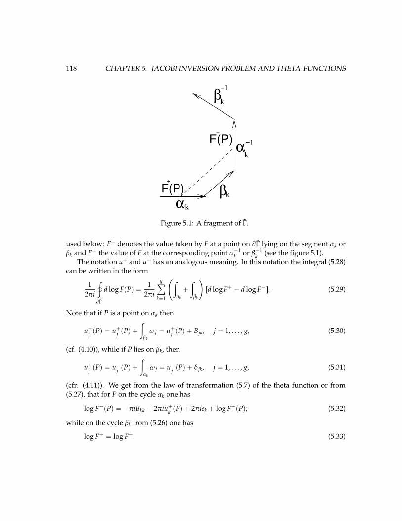
118 CHAPTER 5. JACOBI INVERSION PROBLEM AND THETA-FUNCTIONS
−1
α
α
−1
F(P)−
F(P) +
k
βk
k
βk
Figure 5.1: A fragment of Γ.
used below: F` denotes the value taken by F at a point on BΓ lying on the segment αk orβk and F´ the value of F at the corresponding point α´1
k or β´1k (see the figure 5.1).
The notation u` and u´ has an analogous meaning. In this notation the integral (5.28)can be written in the form
12πi
¿
BΓ
d log FpPq “1
2πi
gÿ
k“1
˜
ż
αk
`
ż
βk
¸
rd log F` ´ d log F´s. (5.29)
Note that if P is a point on αk then
u´j pPq “ u`j pPq `ż
βk
ω j “ u`j pPq ` B jk, j “ 1, . . . , g, (5.30)
(cf. (4.10)), while if P lies on βk, then
u`j pPq “ u´j pPq `ż
αk
ω j “ u´j pPq ` δ jk, j “ 1, . . . , g, (5.31)
(cfr. (4.11)). We get from the law of transformation (5.7) of the theta function or from(5.27), that for P on the cycle αk one has
log F´pPq “ ´πiBkk ´ 2πiu`k pPq ` 2πiek ` log F`pPq; (5.32)
while on the cycle βk from (5.26) one has
log F` “ log F´. (5.33)
5.2. THETA-FUNCTIONS 119
From this on αk
d log F´pPq “ d log F`pPq ´ f rm´eπiomegakpPq, (5.34)
and on βk
d log F´pPq “ d log F`pPq. (5.35)
Accordingly, from (5.34) and (5.34) the sum (5.29) can be written in the form
12πi
¿
BΓ
d log F “ÿ
k
¿
αk
ωk “ g,
where we have used the normalization conditionű
αkωk “ 2πi. The lemma is proved
Note that although the function FpPq is not a single-valued function on Γ, its zerosP1, . . . ,Pg do not depend on the location of the cuts along the canonical basis of cycles.Indeed, if this basis cycles is deformed then the path of integration from P0 to P can changein the formulas for the Abel map. A vector of the form p
ű
γω1, . . . ,ű
γωgq is added to theargument of the theta-function θpzq in (5.25). This is a vector of period lattice tN `MBu.As a result of this the function FpPq can only be multiplied by a non zero factor in view of(5.7).
Now we will show now that the g zeros of FpPq give a solution of the Jacobi inversionproblem for a suitable choice of the vector e.
Theorem 5.13. Let e P Cg, suppose that FpPq “ θpAppq ´ eq ı 0 and P1, . . . ,Pg are its zeros onΓ. Then on the Jacobi variety JpΓq
AgpP1, . . . ,Pgq “ e`K , (5.36)
whereK “ pK1, . . . ,Kgq is the vector of Riemann constants,
K j “ ´1` B j j
2`ÿ
l, j
¨
˝
¿
αl
ωlpPqż P
P0
ω j
˛
‚, j “ 1, . . . , g. (5.37)
Proof. Consider the integral
ζ j “1
2πi
¿
BΓ
u jpPqd log FpPq. (5.38)
This integral is equal to the sum of the residues of the integrands i.e.,
ζ j “ u jpP1q ` ¨ ¨ ¨ ` u jpPgq, (5.39)
120 CHAPTER 5. JACOBI INVERSION PROBLEM AND THETA-FUNCTIONS
where P1, . . . ,Pg are the zeros of FpPq of interest to us. On the other hand, this integralcan be represented by analogy with the proof of Lemma 5.12 in the form
ζ j “1
2πi
gÿ
k“1
˜
ż
αk
`
ż
βk
¸
´
u`j d log F` ´ u´j d log F´q¯
“1
2πi
gÿ
k“1
ż
αk
ru`j d log F` ´ pu`j ` B jkqpd log F` ´ 2πiωkqs
`1
2πi
gÿ
k“1
ż
βk
u`j d log F` ´ pu`j ´ δ jkqd log F`s
“1
2πi
gÿ
k“1
„ż
αk
2πiu`j ωk ´ B jk
ż
ak
d log F` ` 2πiB jk
`1
2πi
ż
b j
d log F`,
in the course of computation we used formula (5.30)-(5.35). The function F takes the samevalues at the endpoints of αk, therefore
ż
αk
d log F` “ 2πink,
where nk is an integer. Further let Q j and Q j be the initial and terminal point of β j. Then
ż
β j
d log F` “ log F`pQ jq ´ log F`pQ jq “
“ logθpApQ jq ` f j ´ eq ´ logθpApQ jq ´ eq “ ´πiB j j ` 2πie j ´ 2πiu jpQ jq,
where f j “ pB1 j, . . . ,Bgjq is a vector of the period lattice. The expression for ζ j can now bewritten in the form
ζ j “ u jpP1q ` ¨ ¨ ¨ ` u jpP jq “
“ e j ´12
B j j ´ u jpQ jq `ÿ
k
ż
a ku jωk `
ÿ
k
B jkp´nk ` 1q. (5.40)
The last two terms can be thrown out, they correspond to the j-coordinate of some vectorof the period lattice. Thus the relation (5.40) coincides with the desired relation (5.36) if itis proved that the constant in this equality reduces to (5.37), i.e.
´12
B j j ´ u jpQ jq `ÿ
k
ż
αk
u jωk “ K j, j “ 1, . . . , g.
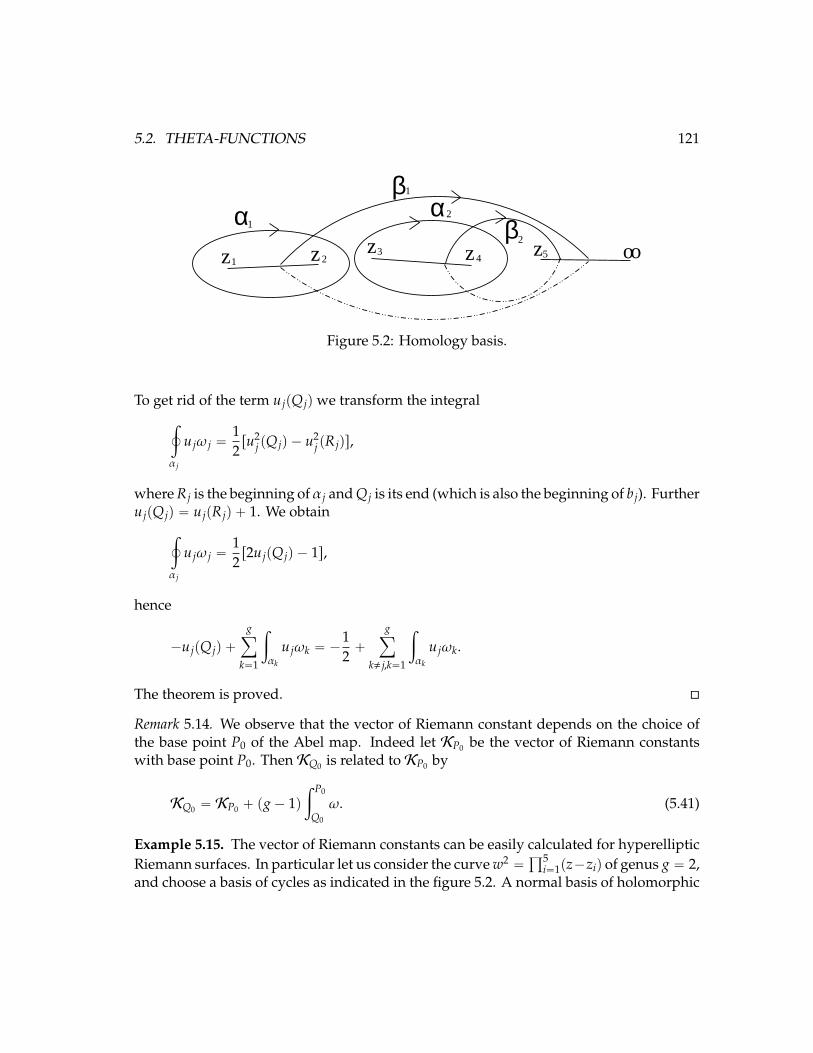
5.2. THETA-FUNCTIONS 121
oozz zz z
βα
βα5
1 23
4
1
1
2
2
Figure 5.2: Homology basis.
To get rid of the term u jpQ jqwe transform the integral¿
α j
u jω j “12ru2
j pQ jq ´ u2j pR jqs,
where R j is the beginning of α j and Q j is its end (which is also the beginning of b j). Furtheru jpQ jq “ u jpR jq ` 1. We obtain
¿
α j
u jω j “12r2u jpQ jq ´ 1s,
hence
´u jpQ jq `
gÿ
k“1
ż
αk
u jωk “ ´12`
gÿ
k, j,k“1
ż
αk
u jωk.
The theorem is proved.
Remark 5.14. We observe that the vector of Riemann constant depends on the choice ofthe base point P0 of the Abel map. Indeed let KP0 be the vector of Riemann constantswith base point P0. ThenKQ0 is related toKP0 by
KQ0 “ KP0 ` pg´ 1qż P0
Q0
ω. (5.41)
Example 5.15. The vector of Riemann constants can be easily calculated for hyperellipticRiemann surfaces. In particular let us consider the curve w2 “
ś5i“1pz´ziq of genus g “ 2,
and choose a basis of cycles as indicated in the figure 5.2. A normal basis of holomorphic
122 CHAPTER 5. JACOBI INVERSION PROBLEM AND THETA-FUNCTIONS
differentials has the form
ω j “
ś2k“1 c jkzk´ldz
w, j “ 1, 2, (5.42)
where the constants c jk are uniquely determined byż
αk
ω j “ δ jk .
We chose as base point of the Abel map the point P0 “ p8,8q. We need to compute¨
˝
¿
α2
ω2pPqż P
P0
ω1
˛
‚,
¨
˝
¿
α1
ω1pPqż P
P0
ω2
˛
‚.
Using the fact that¿
α2
ω2pPqż P
P0
ω1 “
¿
α2
ω2pPqż z4
P0
ω1 `
ż z4
z3
ω2pz,wqż pz,wq
z4
ω1 ´
ż z4
z3
ω2pz,´wqż pz,´wq
z4
ω1
“
¿
α2
ω2pPqż z4
P0
ω1 “
ż z4
P0
ω1 “ p´12´
B12
2q
one obtains
K1 “ ´1` B11
2´
12´
B12
2“ ´1´
B11 ` B12
2
In the same way calculating¿
α1
ω1pPqż P
P0
ω2 “
¿
α1
ω1pPqż z2
P0
ω2 `
ż z2
z1
ω1pz,wqż pz,wq
z2
ω2 ´
ż z2
z1
ω1pz,´wqż pz,´wq
z2
ω2
“
¿
α1
ω1pPqż z2
P0
ω2 “ ´B212
one obtains that
K2 “ ´1` B22 ` B21
2
Observe that the vectorK can be written in the form
K “
ˆ
0,12
˙
`
ˆ
12,
12
˙
B

5.3. THE THETA DIVISOR 123
Namely, given the odd characteristic
p “ˆ
12,
12
˙
, q “ˆ
0,12
˙
,
one has thatK “ q` pB. From this expression it follows that
θpKq “ 0.
It is a general result not restricted to this particular example that θpzq|z“K “ 0.
Corollary 5.16. Let D a positive divisor of degree g. If the function
θpApPq ´ ApDq `Kq
does not vanish identically on Γ then its divisor of zeros coincides with D.
Accordingly, if the function θpApPq ´ eq is not identically equal to zero on Γ, then itszeros give a solution of the Jacobi inversion problem (5.5) for the vector η “ e`K .We haveshown that the map (5.4) Ag : SgΓ Ñ JpΓq is a local homeomorphism in a neighborhoodof a non special positive divisor D of degree g. Since θpzq ı 0 for z P JpΓq, then θpAgpDqqdoes not vanish identically on open subsets of SgΓ. In the next subsection, we characterizethe zero set of the θ-function. The zeros of the theta-function form an analytic subvarietyof JpΓq. The collection of these zeros forms the theta divisor in JpΓq.
5.3 The Theta Divisor
In this section we study the set of zeros of the theta functions and in particular theRiemann vanishing theorem which prescribes in a rather detail manner the set of zerosof the theta-function on Cg.
Theorem 5.17. Let e P Cg, then θpeq “ 0 if and only if e “ ApDg´1q ´ K where Dg´1 is apositive divisor of degree g´ 1 andK is the vector of Riemann constants (5.37).
Remark 5.18. For D P Spg´1qΓ the expression ApDq ´K does not depend on the base pointof the Abel map. The theorem 5.17 says that the theta-function vanishes on a g ´ 1-dimensional variety parametrized by g ´ 1 points of Γ. Defining ApSg´1Γq “ Wg´1 thetheta function vanishes on Wg´1 ´K .
Proof. We first prove sufficiency. Let P1 ` ¨ ¨ ¨ ` Pg be a non special divisor and v “ApP1 ` ¨ ¨ ¨ ` Pgq ´K . Let us consider FpPq “ θpApPq ´ vq. Either F is identically zero ornot. In the former case for each k “ 1, . . . g
FpPkq “ θpApP1 ` ¨ ¨ ¨ ` Pk ` ¨ ¨ ¨ ` Pgq ´Kq “ 0,
124 CHAPTER 5. JACOBI INVERSION PROBLEM AND THETA-FUNCTIONS
where we use the symbol Pk to mean that Pk does not appear in the divisor. So fore “ ApP1 ` ¨ ¨ ¨ ` Pk ` ¨ ¨ ¨ ` Pgq ´K we have θpeq “ 0.
In the latter case FpPq . 0, we have that F has precisely g zeros on Γ due to lemma 5.12.Let Q1, . . .Qg be the zeros of F, then according to theorem 5.13 one has
ApQ1 ` ¨ ¨ ¨ `Qgq “ v`K “ ApP1 ` ¨ ¨ ¨ ` Pgq.
Since P1`¨ ¨ ¨`Pg is not special, it follows from the Riemann-Roch and the Abel theoremsthat Q1` ¨ ¨ ¨ `Qg “ P1` ¨ ¨ ¨ `Pg. Therefore also in this case FpPkq “ θpApP1` ¨ ¨ ¨ ` Pk`
¨ ¨ ¨`Pgq´Kq “ 0 for k “ 1, . . . , g. Since the set of non-special divisor of degree g is densein SpgqΓ, the divisors of the form P1 ` ¨ ¨ ¨ ` Pk ` ¨ ¨ ¨ ` Pg form a dense subset of Spg´1qΓ.Since the function θpzq is continuous, it follows that θpzq is identically zero on Wg´1´K ,where in general Wn Ă JpΓq, is the Abel image of SpnqΓ for n ě 1.
Conversely, let θpeq “ 0. Then by Jacobi inversion theorem, since θ is not identicallyzero on JpΓq. Then there exists an integer s, 1 ď s ď g, so that
θpApD1 ´ D2q ´ eq “ 0, @D1, D2 P Sps´1qΓ
but
θpApD1 ´D2q ´ eq , 0, D1,D2 P SpsqΓ.
Let D1 “ P1 ` ¨ ¨ ¨ ` Ps and D2 “ Q1 ` ¨ ¨ ¨ ` Qs where we assume that the points of thedivisors are mutually distinct. Now let us consider the function
FpPq “ θpApPq ` ApP2 ` ¨ ¨ ¨ ` Psq ´ ApQ1 ` ¨ ¨ ¨ `Qsq ´ eq
Since FpP1q , 0, this function is not identically zero on Γ. Therefore, by theorem 5.13 ithas g zeros on Γ. These zeros are by construction Q1, . . . ,Qs plus some other g´ s pointsTs`1, . . . ,Tg. By theorem 5.13 one has
ApQ1 ` ¨ ¨ ¨ `Qs ` Ts`1,` ¨ ¨ ¨ ` Tgq ´K “ ApQ1 ` ¨ ¨ ¨ `Qsq ´ ApP2 ` ¨ ¨ ¨ ` Psq ` e
or equivalently
e “ ApP2 ` ¨ ¨ ¨ ` Ps ` Ts`1,` ¨ ¨ ¨ ` Tgq ´K
which is a point in Wg´1 ´K .
Regarding the zeros of the theta-function it is possible to prove a little bit more thenstated in the previous theorems. Let D P Spg´1qΓ and let e “ ApDq ´K . Then
multz“eθpzq “ lpDq.
where lpDq is the dimension of the space LpDq. The proof of this identity can be found in[20].
5.3. THE THETA DIVISOR 125
Remark 5.19. The vector of Riemann constants has a characterisation in terms of divisors.Indeed there is a non positive divisor ∆ of degree g´ 1 such that its Abel image coincideswith K , namely Ap∆q “ K . Furthermore let D be a positive divisor of degree g´ 1, thenthe vector
e “ ApDq ´K
is a zero of the theta-function, namely θpeq “ 0. By the parity of the theta-function onehas θp´eq “ 0. It follows by theorem 5.17 that
´e “ ApD1q ´K
where D1 is a positive divisor of degree g ´ 1. Then summing up the two relations weobtain
2K “ ApD`D1q
where D`D1 is a positive divisor of degree 2g´2. It can be proved that the divisor D`Dis the divisor of a holomorphic differential, namely the vector 2K is the Abel image of thedivisor of a differential. More precisely a divisor D is canonical if and only if ApDq “ 2K(see [19] for a proof of these results).
Using the characterization of the theta-divisor one can complete the description of thefunction FpPq.
Lemma 5.20. Let FpPq “ θpApPq ´ eq where e “ ApDq ´ K , D P SpgqΓ and K the vector ofRiemann constants defined in (5.37). Then
1. FpPq ” 0 iff the divisor D is special;
2. FpPq ı 0 iff dimΩpDq “ 0, i.e. the divisort D is not special. In this last case D is the divisorof zeros of FpPq.
Proof. Let’s prove part 1. of the lemma. Let FpPq ” 0, then by theorem 5.17 there is apositive divisor D of degree g´ 1 so that
ApDq ´K ´ ApPq “ ApDq ´K .
By Abel theorem, the identity holds if and only if D and D`P are linearly equivalent, thatis there is a meromorphic function in LpDqwith a zero in an arbitrary point P P Γ. This ispossible only if lpDq ą 1 or equivalently dimΩpDq ą 0, namely D is special. Conversely,if D P SgΓ is special then lpDq ą 1 and therefore there is a function f P LpDq with anarbitrary zero in a point P P Γ so that p f q “ P ` D ´ D. where D P Spg´1qΓ. It followsby Abel theorem that ApPq ´ ApDq ` K “ ´ApDq ` K , then by theorem 5.17, one hasθpApDq ´Kq “ 0.
Now let us prove part 2. of the lemma. Suppose now that D is not special, thenFpPq ı 0 and by theorem 5.13, the divisors of zeros of FpPq coincides with D.
126 CHAPTER 5. JACOBI INVERSION PROBLEM AND THETA-FUNCTIONS
Corollary 5.21. Let e “ ApDq ´K with D P Sg´1Γ. Them the function FpPq “ θpApPq ´ eqvanishes identically if and only if dimΩpD` P0q ě 1 (Check!!) where P0 is the base point of theAbel map.
Proof. Let P0 be the base point of the Abel map, then ApP´P0q “ ApPq. Suppose FpPq ” 0,then by theorem 5.17 there exists a positive divisor D of degree g´ 1 such that
ApP´ P0q ´ ApDq `K “ ´ApDq `K
which implies that ApD ` P0q “ ApD ` Pq. By Abel theorem, there is a nontrivialmeromorphic function h with divisor
phq “ D` P´D´ P0
for all P P Γ. This implies that lpD ` P0q ě 2 or equivalently, D ` P0 is a special divisor.Viceversa suppose that dimΩpD`P0q ě 1, then lpD`P0q ą 1 so that LpD`P0q is generatedby t1, huwhere h is a meromorphic function. So there is a nontrivial meromorphic functionwith poles in D`P0 and having zero in an arbitrary point P ( take for example the functionh´ hpPq) and some other g´ 1 points given by the divisor D. It follows that
ApD` P0q “ ApD` Pq
or equivalently
ApP´ P0q ´ ApDq `K “ ´ApDq ´K
which implies by theorem 5.17 that 0 “ θp´ApDq ´ Kq “ θpApP ´ P0q ´ ApDq ´ Kq “θpApPq ´ ApDq ´Kqwhere we recall that P0 is the base point of the Abel map.
The zeros of the theta function (the points of the theta divisor) form a variety ofdimension 2g ´ 2 (for g ě 3). If we delete from JpΓq, the theta divisor, then we get aconnected 2g-dimensional domain. We get that the Jacobi inversion problem is solvablefor all points of the Jacobian JpΓq and uniquely solvable for almost all points. Thusthe collection pP1, . . . ,Pgq “ pApgqq´1pηq of points of the Riemann surface Γ (withoutconsideration of order) is a single valued function of a point η “ pη1, . . . ηgq P JpΓq (whichhas singularities at points of the theta divisor.) To find an analytic expression for thisfunction we take an arbitrary meromorphic function f pPq on Γ. Then the specification ofthe quantities η1, . . . , ηg uniquely determines the collection of values
f pP1q, . . . , f pPgq, ApgqpP1, . . . ,Pgq “ η. (5.3.43)
Therefore, any symmetric function of f pP1q, . . . , f pPgq is a single-valued meromorphicfunction of the g variables η “ pη1, . . . , ηgq, that is 2g-fold periodic with period lattice
5.3. THE THETA DIVISOR 127
t2πiM` BNu. All these functions can be expressed in terms of a Riemann theta function.The following elementary symmetric functions has an especially simple expression:
σ f pηq “gÿ
j“1
f pP jq. (5.3.44)
From Theorem 5.36 and the residue formula we get for this function the representation
σ f pηq “1
2πi
¿
BΓ
f pPqd logθpApPq ´ η`Kq
´ÿ
f pQkq“8
ResP“Qk
f pPqd logθpApPq ´ η`Kq,(5.3.45)
the second term in the right hand side is the sum of the residue of the integrand over allpoles if f pPq. As in the proof of Lemma 5.12 and Lemma 5.13, it is possible to transformthe first term in (5.3.45) by using the formulas (5.34) and (5.35). The equality (5.3.45) canbe written in the form
σ f pηq “1
2πi
ÿ
k
ż
ak
f pPqωk ´ÿ
f pakq“8
ResP“Qk
f pPqd logθpApPq ´ η`Kq. (5.3.46)
Here the first term is a constant independent of η. We analyze the computation of thesecond term (the sum of residue) using an example.
Example 5.22. Γ is an hyperelliptic Riemann surface of genus g given by the equationw2 “ P2g`1pzq, and the function f has the form f pz,wq “ z, the projection on the z-plane.This function on Γ has a unique two-fold pole at8. We get an analytic expression for thefunction σ f constructed according to the formula (5.3.44). In other words if P1 “ pz1,w1q,. . . ,Pg “ pzg,wgq is a solution of the inversion problem ApP1q ` ¨ ¨ ¨ ` ApPgq “ η, then
σ f pηq “ z1 ` ¨ ¨ ¨ ` zg. (5.3.47)
We take 8 as the base point P0 (the lower limit in the Abel mapping). According to(5.3.46) the function σ f pηq has the form
σ f pηq “ c´ Res8rzd logθpApPq ´ η`Kqs .
Let us compute the residue. Take τ “ z´12 as a local parameter in a neighborhood
of 8. Suppose that the holomorphic differentials ωi have the form ωi “ ψipτqdτ in a
128 CHAPTER 5. JACOBI INVERSION PROBLEM AND THETA-FUNCTIONS
neighborhood of8. Then
d logθpApPq ´ η`Kq “gÿ
i“1
rlogθpApPq ´ η`KsiωipPq “
“
gÿ
i“1
rlogθpApPq ´ η`Kqsiψipτqdτ
where r. . . si denotes the partial derivative with respect to the ith variable. By the choiceof the base point point P0 “ 8, the decomposition of the vector-valued function ApPq ina neighborhood of8 has the form
ApPq “ τU `Opτ2q,
where the vector U “ pU1, . . . ,Ugq has the form
U j “ ψ jp0q, j “ 1, . . . , g.
From these formulas we finally get
σ f pηq “ ´plogθpη´Kqqi, jUiU j ` c “ ´B2x logθpxU ` η´Kq|x“0 ` c, (5.3.48)
where plogθpη´Kqqi, j denotes derivative with respect to the i´ th and j´ th argumentof the theta-function and c is a constant.
We shall show in the next Section that the function
upx, tq “B2
Bx2 logθpUx`Wt´ η`Kq ` c
where Wk “13ψ2p0q solves the Korteweg de Vries equation
ut “14p6uux ` uxxxq.
Exercise 5.23: Suppose that a hyperelliptic Riemann surface of genus g is given by theequation w2 “ P2g`2pzq. Denotes its points at infinity by P´ and P`. Chose P´ as the basepoint P0 of the Abel mapping. Take f pz,wq “ z as the function f . Prove that the functionσ f pηq has the form
σ f pηq “
ˆ
logθpη´K ´ ApP`qq
θpη´Kq
˙
jU j ` c (5.3.49)
5.3. THE THETA DIVISOR 129
where the vector U “ pU1, . . . ,Ugq has the form
U j “ ψ jp0q, j “ 1, . . . , g, (5.3.50)
where the basis of holomorphic differentials have the form
ω jpPq “ ψ jpτqdτ, τ “ z´1, P Ñ8.
Exercise 5.24: Let Γ be a Riemann surface w2 “ P5pzq of genus 2. Consider the twosystems of differential equations:
dz1
dx“
a
P5pz1q
z1 ´ z2,
dz2
dx“
a
P5pz2q
z2 ´ z1(5.3.51)
dz1
dt“
z2a
P5pz1q
z1 ´ z2,
dz2
dt“
z1a
P5pz2q
z2 ´ z1. (5.3.52)
Each of these systems determined a law of motion of the pair of points
P1 “ pz1,b
P5pz1qq, P2 “ pz2,b
P5pz2qq
on the Riemann surface Γ. Prove that under the Abel mapping (5.1) these systems passinto the systems with constant coefficients
dη1
dx“ 0,
dη2
dt“ 1
dη1
dt“ ´1,
dη2
dt“ 0.
In other words, the Abel mapping (5.1) is simply a substitution integrating the equations(5.3.51) and (5.3.52).
130 CHAPTER 5. JACOBI INVERSION PROBLEM AND THETA-FUNCTIONS
Bibliography
[1] Ahiezer, N. I. Continuous analogues of orthogonal polynomials on a system ofintervals. (Russian) Dokl. Akad. Nauk SSSR 141 (1961) 263–266.
[2] Ahiezer, N. I. Elements of the theory of elliptic functions [Second revised edition]Izdat. “Nauka”, Moscow 1970 304 pp.
[3] Erdelyi, Arthur; Magnus, Wilhelm; Oberhettinger, Fritz; Tricomi, Francesco G.Higher transcendental functions. Vol. II. Based on notes left by Harry Bateman.Reprint of the 1953 original. Robert E. Krieger Publishing Co., Inc., Melbourne, Fla.,1981.
[4] Veselov, A. P. Finite-zone potentials and integrable systems on a sphere withquadratic potential. (Russian) Funktsional. Anal. i Prilozhen. 14 (1980), no. 1, 48–50.
[5] Golubev, V. V. (Russian) [Lectures on the integration of the equations of motion of aheavy rigid body about a fixed point.] Gosudarstv. Izdat. Tehn.-Teor. Lit., Moscow,1953. 287 pp.
[6] Griffiths, Phillip; Harris, Joseph Principles of algebraic geometry. Reprint of the 1978original. Wiley Classics Library. John Wiley and Sons, Inc., New York, 1994.
[7] Hurwitz, Adolf; Courant, R. Vorlesungen ber allgemeine Funktionentheorie undelliptische Funktionen. (German) Interscience Publishers, Inc., New York, (1944).
[8]
[9] Dubrovin, B. A.; Fomenko, A. T.; Novikov, S. P. Modern geometry—methods andapplications. Part I and Part II. Translated from the Russian by Robert G. Burns.Graduate Texts in Mathematics, 104. Springer-Verlag, New York, 1984 -1985.
[10] Dubrovin, B. A.; Fomenko, A. T.; Novikov, S. P. Modern geometry—methods andapplications. Part III. Introduction to homology theory. Translated from the Russian
131
132 BIBLIOGRAPHY
by Robert G. Burns. Graduate Texts in Mathematics, 124. Springer-Verlag, New York,1990.
[11] Zaharov, V. E.; Shabat, A. B. Integration of the nonlinear equations of mathematicalphysics by the method of the inverse scattering problem. II. (Russian) Funktsional.Anal. i Prilozhen. 13 (1979), no. 3, 13–22.
[12] Farkas, Hershel M.; Kra, Irwin Theta constants, Riemann surfaces and the modu-lar group. An introduction with applications to uniformization theorems, partitionidentities and combinatorial number theory. Graduate Studies in Mathematics, 37.
[13] G. Fischer, Plane algebraic curves. Translated from the 1994 German original by LeslieKay. Student Mathematical Library, 15. American Mathematical Society, Providence,RI, 2001. xvi+229 pp.
[14] O.Forster, Lectures on Riemann surfaces. Translated from the German by Bruce Gilligan.Graduate Texts in Mathematics, 81. Springer-Verlag, New York-Berlin, 1981. viii+254pp.
[15] Kirwan, Frances Complex algebraic curves. London Mathematical Society StudentTexts, 23. Cambridge University Press, Cambridge, 1992. viii+264 pp.
[16] Griffiths, Phillip; Harris, Joseph Principles of algebraic geometry. Reprint of the 1978original. Wiley Classics Library. John Wiley and Sons, Inc., New York, 1994. xiv+813pp.
[17] Donaldson, Simon Riemann surfaces. Oxford Graduate Texts in Mathematics, 22.Oxford University Press, Oxford, 2011. xiv+286 pp.
[18] Springer, George Introduction to Riemann surfaces. Addison-Wesley Publishing Com-pany, Inc., Reading, Mass. 1957.
[19] Fay, John D. Theta functions on Riemann surfaces. Lecture Notes in Mathematics,Vol. 352. Springer-Verlag, Berlin-New York, 1973. iv+137 pp.
[20] Farkas, H. M.; Kra, I. Riemann surfaces. Second edition. Graduate Texts in Mathe-matics, 71. Springer-Verlag, New York, 1992. xvi+363 pp.
[21] Lewittes, J., Riernann surfaces and the theta functions. Acta Math. 111 (1964) 3761.