rights / license: research collection in copyright - non ...30231/... · models are of special...

Research Collection

Conference Paper

Recent developments regarding similarities in transportmodelling

Author(s): Schüssler, Nadine; Axhausen, Kay W.

Publication Date: 2007

Permanent Link: https://doi.org/10.3929/ethz-a-005563058

Rights / License: In Copyright - Non-Commercial Use Permitted

This page was generated automatically upon download from the ETH Zurich Research Collection. For moreinformation please consult the Terms of use.

ETH Library

https://doi.org/10.3929/ethz-a-005563058

http://rightsstatements.org/page/InC-NC/1.0/

https://www.research-collection.ethz.ch

https://www.research-collection.ethz.ch/terms-of-use

Recent developments regarding similarities intransport modelling

Nadine SchuesslerKay W. Axhausen

STRC 2007 August 2007

Recent developments regarding similarities in transport modelling August 2007

STRC 2007

Recent developments regarding similarities in transport mod-ellingNadine SchuesslerIVTETH ZürichCH-8093 Zürichphone: +41-44-633 30 85fax: +41-44-633 10 [email protected]

Kay W. AxhausenIVTETH ZürichCH-8093 Zürichphone: +41-44-633 39 43fax: +41-44-633 10 [email protected]

August 2007

Abstract

Overcoming the independence of irrelevant alternatives (IIA) property of the basic MultinomialLogit (MNL) model is a major research issue in the field of discrete choice modelling. In recentyears, several approaches have been developed to achieve this goal with different degrees ofappropriateness.

On the one hand there are very flexible models, which are able to account for complex corre-lation structures and a wide variety of interdependencies between alternatives by opening thevariance-covariance structure. But they require a lot of effort in terms of specification and com-putation. On the other hand there are less complex models, which introduce a similarity factorinto the systematic part of the utility function, which decreases the utility of an alternative withrespect to its similarity with other alternatives. They are easier to estimate and applicable tolarge choice sets. However, these models were designed to solve specific, in particular routechoice, problems and not offhand transferable.

This paper summarises and evaluates different approaches to overcome the IIA property. Spe-cial consideration is given to approaches that are easy to compute and applicable to a combinedroute, mode and destination choice model.

KeywordsDiscrete choice, IIA property, similarities

1


1 Introduction

Today discrete choice models have manifold applications. They are used in a wide variety ofcontexts to simulate consumer choice. They are based on the idea that a decision-maker isconfronted with a set of discrete alternatives and has to choose one of them. The model itselfestimates for each alternative the probability of being chosen assuming that a decision-makerseek to maximise his or her utility. The utility depends on the decision-maker’s individual pref-erences, the choice situation, the characteristics of the alternative and its similarities with theother available alternatives. The underlying utility function is split into two elements: a sys-tematic part and a random part, for both of which the analyst has to make suitable distributionalassumptions. In principle, the analyst is free from a priori constraints in his or her choice ofapproach to capture similarities among alternatives. Similarities can be included in the system-atic part through a suitable measure of similarity or through an appropriate specification of thevariance-covariance matrix of the random part.

Either approach, with different degrees of appropriateness, overcomes the "Independence ofIrrelevant Alternatives" (IIA) property of the basic Multinomial Logit (MNL) model. Thisproperty implies that the ratio of the choice probabilities of any two alternatives is not affectedby the availability or the attributes of other alternatives and is therefore independent of the sizeand structure of the choice set. Not correcting for the IIA property leads in many cases to - very- misleading model results and forecasts.

Recent research has developed several approaches to overcome this structural problem, butnone is completely satisfactory. On the one hand there are very flexible models, which areable to describe complex correlation structures of the error terms. They account for a widevariety of interdependencies between alternatives by opening the variance-covariance structureof the model. But they require a lot of effort in terms of specification and computation and arenot obviously suitable for large sets of overlapping alternatives. This is especially a problemin the field of transport research. Realistic problems addressed here are often characterisedby large sets of alternatives as for example in route or destination choice. For models thatsimultaneously address two or more choices this problem increases even further; think forexample of a joint destination and route choice model.

On the other hand there are less complex models, which are easier to estimate and applicable tolarge choice sets. However, these were designed to solve specific problems and are not offhandtransferable. They introduce a similarity factor to the systematic part of the utility function,which adjusts the utility of an alternative with respect to its similarity with other alternatives.The majority of these models has been developed for route choice, though some applicationsfor destination and location choice have been proposed. Nevertheless, there have hardly beenany approaches for dealing with multi-modal situations or other combined choice problems.

2


This paper summarises and evaluates different approaches to overcome the IIA property. First,an introduction to the MNL model and its IIA property and to the idea of the different ap-proaches is given. Subsequently, the approaches that subdivide alternatives into nests are in-troduced before those changing the variance-covariance structure and the ones that introducesimilarity factors in the deterministic part of the utility function are presented. The paper con-cludes with a discussion of the different approaches and an outlook for future research. Specialconsideration is given to question if they are applicable to a combined route, mode and desti-nation choice model.

3


2 The MNL model and its IIA property

Discrete choice models are a standard for modelling consumer behaviour. In transport research,they are used for all aspects of travel behaviour, including, but not limited to household activ-ity scheduling, destination choice, route choice and mode choice. Therefore, discrete choicemodels are of special importance for the evaluation of transport policies, such as infrastructureinvestment or setting of tolls.

In a discrete choice model, an individual - the decision-maker - is confronted with a set of dis-crete alternatives, the choice set, from which he or she has to choose one. As a decision rule,it is assumed that the decision-maker seeks to maximise his or her personal utility. The utilityof each alternative is characterised by its measurable attributes captured by the deterministiccomponent Vin of the utility function. Beyond that, there are utility components that cannotbe measured directly due to several reasons. First, there is heterogeneity of preferences acrossdecision-makers. Second, the knowledge and the information processing abilities of decision-makers are limited. Third, there are further uncertainties regarding the choice process, includ-ing attributes which the analyst is not able or not resourced to measure. These elements areusually represented by the random term εin of the utility function. Thus, the following utilityfunction is postulated:

Uin = Vin + εin (1)

with Vin being defined as Vin = f(β, xin) , where β is a vector of taste coefficients, and xin avector of the attributes of alternative i as faced by respondent n in the specific choice situation.In addition, socio-demographic attributes of respondent n can be included in the systematicpart of the utility function.

The discrete choice model itself estimates for each alternative the probability of being chosenfrom a given choice set:

P (i|Cn) = P [Uin ≥ Ujn,∀j ∈ Cn] (2)

The most commonly used discrete choice model is the Multinomial Logit Model (MNL) pro-posed by McFadden (1974). It is based on the assumption that the random terms, often callederror terms, are identically and independently (i.i.d.) Gumbel distributed. The choice probabil-ity of each alternative i can then be calculated as:

P (i|Cn) =eµVin∑j e

µVjn(3)

Thereby, µ is related to the standard deviation of the Gumbel variable (µ2 = π6σ2 ), where, in

4


the absence of a heterogeneous population, µ is generally constrained to a value of 1.

The advantages of the MNL model are its flexibility in terms of its deterrence sensitivity, andthe ease of the parameter estimation (c.f. Ben-Akiva and Lerman (1985)). On the other hand,the MNL model has several disadvantages, the most prominent being the Independence from

Irrelevant Alternatives (IIA) property: The relative ratio of the choice probabilities of twoalternatives does not depend on the existence or the characteristics of other choice alternatives.

P (i|Cn)

P (k|Cn)=

eµVin∑j eµVjn

eµVkn∑j eµVjn

= eµ(Vin−Vkn) (4)

An illustration for this problem is the well-known red bus/blue bus paradox (Debreu, 1960),which describes two mode choice situations. First, the decision-maker is facing two alterna-tives: taking the car or a red bus. It is assumed, that each alternative has a choice probability of50%. In the second scenario, a blue bus with the same attributes relevant for the decision as thered bus is added to the choice set. Because the new alternative is just another option for usingpublic transport, one would expect, that the share of the additional alternative comes completelyat the expense of the red bus and the resulting choice probabilities should be: PCar = 50%,Predbus = 25% and Pbluebus = 25% – ignoring for now the potential mode shift because ofincreased frequencies on the bus network. However, because of the IIA property, the MNLreturns the same choice probability for each alternative (PCar = 33%, Predbus = 33% andPbluebus = 33%) to guarantee that the ratio between the probabilities for the car and the red busstays equal to one.

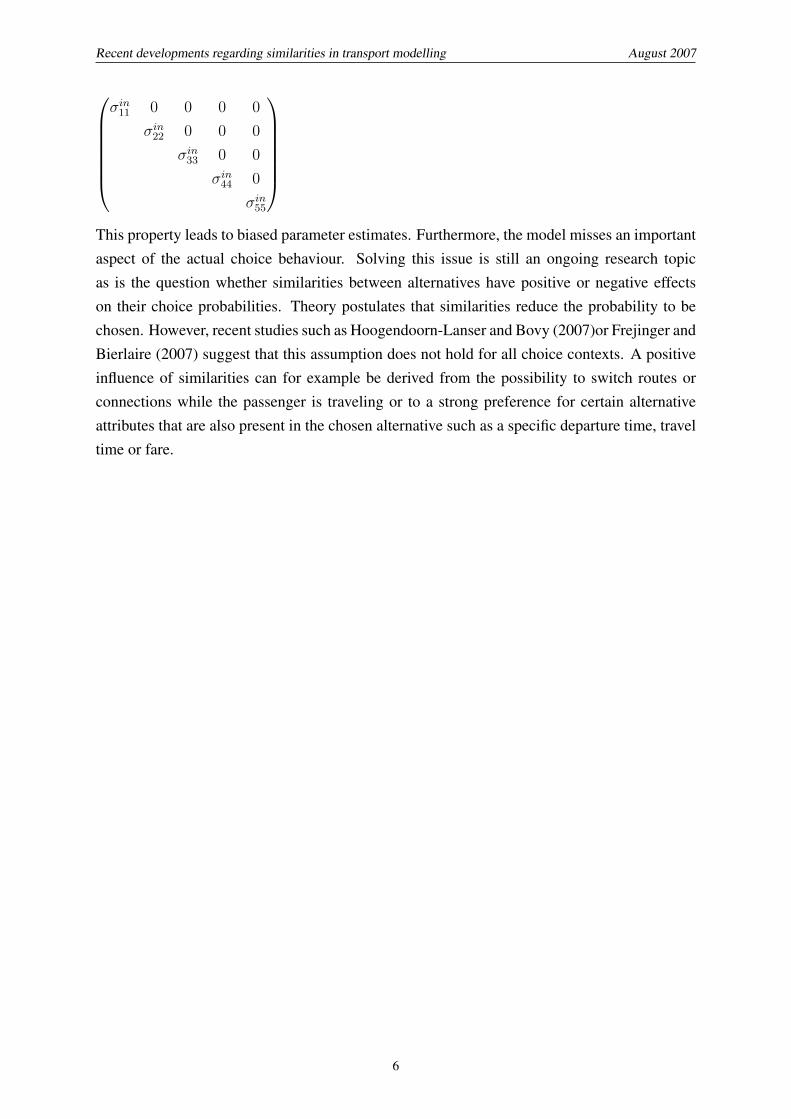
Though the red bus and the blue bus obviously share a lot of characteristics and are thereforesimilar, the MNL model ignores this completely. The same applies for any other choice con-text, as demonstrated for example by Daganzo and Sheffi (1977) for private transport routechoice, where the similarity between routes is derived from their overlap. Thus, one possibleinterpretation of the IIA property of the MNL model is its failure account for similarities be-tween alternatives. Mathematically, similarities can be represented by correlations. Since theerror terms in the MNL model are independently distributed, no correlations are included inthe model as can be seen from the variance-covariance matrix for 5 alternatives depicted be-low, where because of its immanent symmetry, only the upper triangle of the matrix is shown.The matrix consists only of the variances of the alternatives’ utilities. The covariances are allassumed to be equal to zero.

5


σin11 0 0 0 0

σin22 0 0 0

σin33 0 0

σin44 0

σin55

This property leads to biased parameter estimates. Furthermore, the model misses an importantaspect of the actual choice behaviour. Solving this issue is still an ongoing research topicas is the question whether similarities between alternatives have positive or negative effectson their choice probabilities. Theory postulates that similarities reduce the probability to bechosen. However, recent studies such as Hoogendoorn-Lanser and Bovy (2007)or Frejinger andBierlaire (2007) suggest that this assumption does not hold for all choice contexts. A positiveinfluence of similarities can for example be derived from the possibility to switch routes orconnections while the passenger is traveling or to a strong preference for certain alternativeattributes that are also present in the chosen alternative such as a specific departure time, traveltime or fare.

6


3 Accounting for similarities between discrete choice alter-natives

Before exploring the different approaches of how to handle similarities in discrete choice mod-elling, one has to reflect, what kind of similarities can appear in real choice situations, asthey can differ enormously depending on the decision context. Considering for example modechoice, similarities between private or public transport modes can lie in characteristics such asaccessibility, comfort or levels of privacy. Correlations between private transport routes appear,if routes share links, whereas similarities among public transport connections are determinedthrough comparable time slots or journey times, equal interchange facilities or the same oper-ator. An individual facing a destination choice problem has to deal with even more possiblesimilarities. Those can include the geographic region, the landscape, the journey direction(route overlap), the weather, the products/services offered or shared parking sites - to nameonly a few.

Gower (1985) provides the definition of a general measure of similarity as well as a descriptionof its properties and its applicability to different types of variables. In his measure the similaritybetween two alternatives is determined by comparing each of their attributes, assigning a scorefor the degree of similarity and combining those scores to a single number. Below, a shortdescription of similarity scores for single-level variables of different variable types is followedby the introduction of Gower’s general similarity measure that combines them.

Dichotomous and categorial variables can be treated in a similar way. While dichotomousvariables represent the presence or absence of a characteristic, categorial variables embodyqualities of equal standing. The similarity score for those variables can only be unity or zerodepending on the question, if they are equal or not. Care must however be taken with regard tothe question if the absence of both attributes of a dichotomous variable is considered as equalityor not. The similarity or dissimilarity between quantitative variables can be measured throughthe distance between their attributes. This distance is then converted into a fraction betweenzero and unity to get the score for the similarity measure.

Gower (1985) then combines the similarity scores sk(xik, xjk) of the individual variables to the"General Coefficient of Similarity" between the alternatives i and j, which has the followingfunctional form

Sij =

∑pk=1 wk(xik, xjk) · sk(xik, xjk)∑p

k=1 wk(xik, xjk)(5)

Thereby the function imposed for sk(xik, xjk) can differ for each variable. wk(xik, xjk) rep-resents the weight put on the individual attribute to reflect the importance of a variable or itsreliability.

7


With the help of this approach even hierarchies of alternatives can be compared in the way thatthe similarity score S(k)

ij of the secondary alternatives associated to attribute k is imposed asweight for the primary variable (c.f. Gower (1985), p. 400):

Sij =

p∑k=1

Skij(xik, xjk) · sk(xik, xjk) (6)

Any depth of nesting can be represented by generalising this procedure.

There are different ways of describing similarities between alternatives. Three general ap-proaches can be distinguished that will be described in the following sections:

• subdividing alternatives into nests,

• opening the variance-covariance structure, and

• introducing similarity factors in the deterministic part of the utility function.

The first group basically contains the Multivariate Extreme Value (MEV) models other thanthe MNL model. The alternatives are subdivided into groups, called nests. Correlations mayremain within the nests, but between the nests they are eliminated. In the Nested Logit (NL)model the nests are completely disjoint whereas in the Cross Nested Logit (CNL) model eachalternative can belong to more than one nest. However, though particularly the CNL is ableto represent nearly all kinds of correlations, a realistic nesting structure is highly complex andtherefore cumbersome to estimate.

Most of recent research efforts have however focussed on the second group of models, morespecifically on the Mixed Multinomial Logit (MMNL) Models. Inspired by the MultinomialProbit Model where multivariate normally distributed error terms replace the i.i.d. Gumbeldistributed ones of the MNL model, in an MMNL model the deterministic part of the utilityfunction is re-formulated while the i.i.d. Gumbel error terms remain. A multivariate randomlydistributed error term is introduced that captures similarities which cannot be modelled deter-ministically. This leads to models that are able to account for any kind of correlation structureand taste heterogeneity. However, these models require a lot of effort in terms of specification,identification and computation and are thus still hardly applicable to choice situations withlarge numbers of alternatives.

The models of the third group aim to capture correlation effects by correcting the systematiccomponent of the utility function. Based on the implicit availability/perception model (IAP)presented by Cascetta et al. (1996) they rest upon the assumption that the utility of an alternativeis decreased by its degree of similarity with other alternatives. Thus, they add a deterministicsimilarity measure to the utility function. Again, the deterministic part is reformulated and

8


the error terms remain i.i.d. Gumbel distributed. The crucial aspect of these approaches is theappropriate choice of the similarity factor. Alternatives in transport choice problems are usuallycharacterised by attributes of different variable type. Hence, a suitable similarity measure has tocope with different variable types, such as dichotomous, categorial and quantitative variables.

9


4 Multivariate Extreme Value models

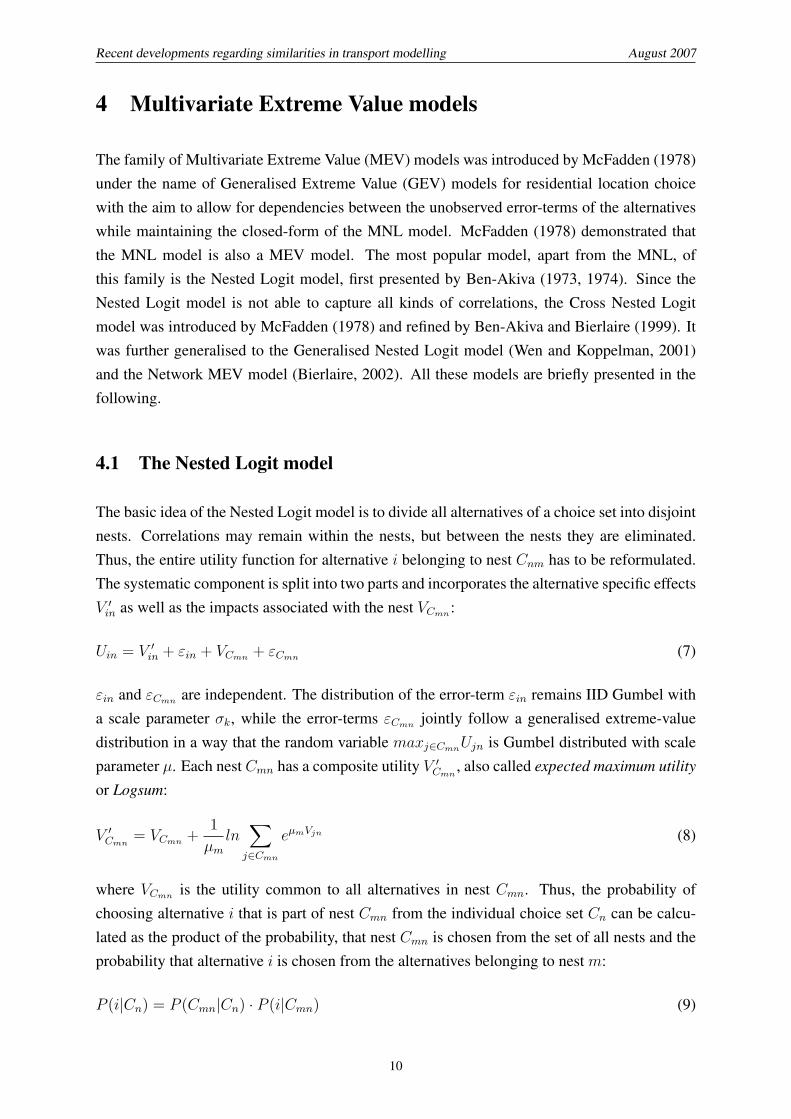
The family of Multivariate Extreme Value (MEV) models was introduced by McFadden (1978)under the name of Generalised Extreme Value (GEV) models for residential location choicewith the aim to allow for dependencies between the unobserved error-terms of the alternativeswhile maintaining the closed-form of the MNL model. McFadden (1978) demonstrated thatthe MNL model is also a MEV model. The most popular model, apart from the MNL, ofthis family is the Nested Logit model, first presented by Ben-Akiva (1973, 1974). Since theNested Logit model is not able to capture all kinds of correlations, the Cross Nested Logitmodel was introduced by McFadden (1978) and refined by Ben-Akiva and Bierlaire (1999). Itwas further generalised to the Generalised Nested Logit model (Wen and Koppelman, 2001)and the Network MEV model (Bierlaire, 2002). All these models are briefly presented in thefollowing.

4.1 The Nested Logit model

The basic idea of the Nested Logit model is to divide all alternatives of a choice set into disjointnests. Correlations may remain within the nests, but between the nests they are eliminated.Thus, the entire utility function for alternative i belonging to nest Cnm has to be reformulated.The systematic component is split into two parts and incorporates the alternative specific effectsV ′in as well as the impacts associated with the nest VCmn:

Uin = V ′in + εin + VCmn + εCmn (7)

εin and εCmn are independent. The distribution of the error-term εin remains IID Gumbel witha scale parameter σk, while the error-terms εCmn jointly follow a generalised extreme-valuedistribution in a way that the random variable maxj∈CmnUjn is Gumbel distributed with scaleparameter µ. Each nest Cmn has a composite utility V ′Cmn , also called expected maximum utility

or Logsum:

V ′Cmn = VCmn +1

µmln∑j∈Cmn

eµmVjn (8)

where VCmn is the utility common to all alternatives in nest Cmn. Thus, the probability ofchoosing alternative i that is part of nest Cmn from the individual choice set Cn can be calcu-lated as the product of the probability, that nest Cmn is chosen from the set of all nests and theprobability that alternative i is chosen from the alternatives belonging to nest m:

P (i|Cn) = P (Cmn|Cn) · P (i|Cmn) (9)

10


with

P (Cmn|Cn) =eµV

′Cmn∑M

l=1 eµV ′Cln

(10)

and

P (i|Cmn) =eµmVin∑

j∈Cmn eµmVjn

(11)

For µµm

= 1 ∀k the NL collapses to the MNL model.

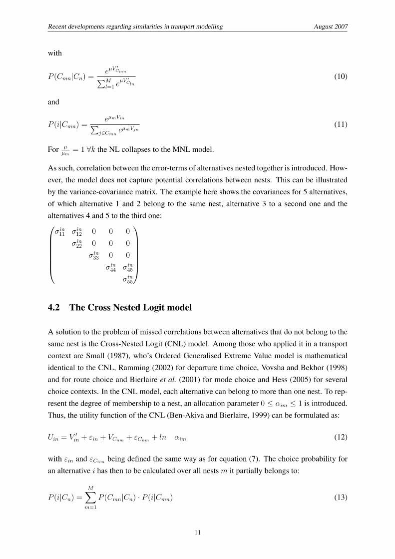
As such, correlation between the error-terms of alternatives nested together is introduced. How-ever, the model does not capture potential correlations between nests. This can be illustratedby the variance-covariance matrix. The example here shows the covariances for 5 alternatives,of which alternative 1 and 2 belong to the same nest, alternative 3 to a second one and thealternatives 4 and 5 to the third one:σin11 σin12 0 0 0

σin22 0 0 0

σin33 0 0

σin44 σin45

σin55

4.2 The Cross Nested Logit model

A solution to the problem of missed correlations between alternatives that do not belong to thesame nest is the Cross-Nested Logit (CNL) model. Among those who applied it in a transportcontext are Small (1987), who’s Ordered Generalised Extreme Value model is mathematicalidentical to the CNL, Ramming (2002) for departure time choice, Vovsha and Bekhor (1998)and for route choice and Bierlaire et al. (2001) for mode choice and Hess (2005) for severalchoice contexts. In the CNL model, each alternative can belong to more than one nest. To rep-resent the degree of membership to a nest, an allocation parameter 0 ≤ αim ≤ 1 is introduced.Thus, the utility function of the CNL (Ben-Akiva and Bierlaire, 1999) can be formulated as:

Uin = V ′in + εin + VCnm + εCnm + ln αim (12)

with εin and εCnm being defined the same way as for equation (7). The choice probability foran alternative i has then to be calculated over all nests m it partially belongs to:

P (i|Cn) =M∑m=1

P (Cmn|Cn) · P (i|Cmn) (13)

11


It is important to note, that any functional relationship can be defined for the allocation param-eter αim depending on the choice context, though often, simple point-estimates are used. Abbeet al. (2007) derived a normalisation for αim which is:∑m

αµµmim = c,∀j ∈ Cn (14)

where c is a constant that does not depend on i.

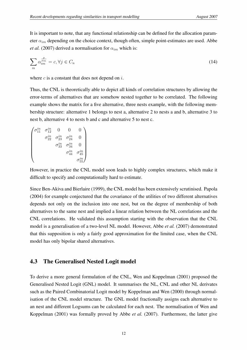
Thus, the CNL is theoretically able to depict all kinds of correlation structures by allowing theerror-terms of alternatives that are somehow nested together to be correlated. The followingexample shows the matrix for a five alternative, three nests example, with the following mem-bership structure: alternative 1 belongs to nest a, alternative 2 to nests a and b, alternative 3 tonest b, alternative 4 to nests b and c and alternative 5 to nest c.σin11 σin12 0 0 0

σin22 σin23 σin24 0

σin33 σin34 0

σin44 σin45

σin55

However, in practice the CNL model soon leads to highly complex structures, which make itdifficult to specify and computationally hard to estimate.

Since Ben-Akiva and Bierlaire (1999), the CNL model has been extensively scrutinised. Papola(2004) for example conjectured that the covariance of the utilities of two different alternativesdepends not only on the inclusion into one nest, but on the degree of membership of bothalternatives to the same nest and implied a linear relation between the NL correlations and theCNL correlations. He validated this assumption starting with the observation that the CNLmodel is a generalisation of a two-level NL model. However, Abbe et al. (2007) demonstratedthat this supposition is only a fairly good approximation for the limited case, when the CNLmodel has only bipolar shared alternatives.

4.3 The Generalised Nested Logit model

To derive a more general formulation of the CNL, Wen and Koppelman (2001) proposed theGeneralised Nested Logit (GNL) model. It summarises the NL, CNL and other NL derivatessuch as the Paired Combinatorial Logit model by Koppelman and Wen (2000) through normal-isation of the CNL model structure. The GNL model fractionally assigns each alternative toan nest and different Logsums can be calculated for each nest. The normalisation of Wen andKoppelman (2001) was formally proved by Abbe et al. (2007). Furthermore, the latter give

12


guidance to derive a CNL model from any arbitrary variance-covariance structure.

4.4 The Network MEV model

Another approach of generalisation was proposed by Bierlaire (2002) with the Network MEVmodel. The author showed that any correlation structure represented by a network with certainproperties can be modelled with a NGEV model and furthermore, that every such model isindeed a MEV model. Thereby, the properties for the network are straightforward: The net-work is not allowed to include circuits, it has to have one root node without predecessors, thealternatives have to be represented by leafs without successors, and each node in the networkhas to be part of a continuous path between the root and one alternative. This model formula-tion is especially appealing because of its intuitive way of capturing even complex correlationstructures. It eases the formulation of a complex model by its recursive definition.

13


5 Probit and Mixed Multinomial Logit models

Recently, it has been popular to develop discrete choice models that overcome the IIA propertyby opening the variance-covariance structure. The most extensive of these models is the Multi-nomial Probit model. Mixed Multinomial Logit models aim to combine Probit-like error termswith the closed-form of the MNL model. Both model forms are briefly described in the fol-lowing. Subsequently several studies that successfully employed MMNL models to transportchoice problems are presented.

5.1 The Probit model

In the Probit model, discussed for example by Daganzo (1979), multivariate Normal distributederror terms replace the i.i.d. Gumbel distributed ones of the MNL resulting in the most generalvariance-covariance structure:σin11 σin12 σin13 σin14 σin15

σin22 σin23 σin24 σin25

σin33 σin34 σin35

σin44 σin45

σin55

Thus, any variance-covariance structure can be specified and all kinds of correlation structuresbetween the alternatives of the choice set can be depicted. Probit model have for example beenapplied by Yai et al. (1997) or Daganzo and Sheffi (1977) to private transport route choice prob-lems. The respective authors specified models, in which the covariances of the route utilitiesare proportional to the length of link overlaps. However, the formulation of the Probit model iscomplex and its choice probabilities do not have a closed form. It can not be solved analyticallyand requires simulation for estimation as well as application. Thus, it is only applicable if thenumber of parameters and alternatives is small.

5.2 The Mixed Multinomial Logit models

The family of Mixed Multinomial Logit (MMNL) or Logit Kernel (LK) models was proposedby Walker (2001) with the aim to combine the advantages of a Probit model with those of aLogit model. MMNL models do also belong to the family of MEV models. However, sincethey apply a different approach to capture similarities they are dealt with separately in thispaper.

Two conceptually different but mathematically identical approaches of the MMNL model exist:

14


the Error-Components Logit (ECL) and the Random-Coefficients Logit (RCL). In the ECLmodel the systematic part Vin of the utility function is split into a deterministic componentV ′in and a random error component ηin. ηin is generally assumed to be multivariate Normaldistributed. Correlation is introduced by allowing some alternatives to share the same errorcomponent. The RCL model accommodates unobserved variation across individuals in theirsensitivity to observed exogenous variables by specifying some entries of the vector β in theequation Vin = f(β, xin) to be random variables. This can also be represented by adding amultivariate Normal distributed variable ηin to the utility function. Thus, for the ECL as wellas the RCL model the utility function can be denoted as follows:

Uin = V ′in + ηin + εin (15)

V ′in is re-formulated using only the attributes of the alternatives, the decision maker and thechoice situation while ηin is a multivariate randomly distributed error term that captures simi-larities which cannot be modelled deterministically.

In the present context, the ECL approach is of special interest. By specifying the structure ofthe error-components such that a given set of alternative shares an error-component, correlationbetween these alternatives is allowed for. In theory, the resulting model can approximate anycorrelation structure, including heteroscedastic ones, arbitrarily closely. As such, the modelcan also replicate the variance-covariance matrix of the general Probit model. Like the Pro-bit model, the ECL model has the disadvantage that simulation is required in estimation andapplication. In addition, imposing the right identification restrictions so that a unique solutioncan be obtained from the infinite set of optimal solutions of the unconstrained model is a diffi-cult and time-consuming task and an often overlooked one as argued in Walker (2002). If theMMNL model additionally allows for random taste variation (e.g. in an RCL framework), theseproblems go much further because before identification issues can be solved, the appropriatedistribution function for the random parameters has to be determined. This altogether makesthe model difficult to be applied in large-scale forecasting systems. For further discussion seeWalker (2002), Walker et al. (2007) and Ben-Akiva and Bolduc (1996).

Yet, several studies have successfully applied MMNL models to transport related choice prob-lems. Private transport route choice problems have for example been examined by Bekhor et al.

(2001), Ramming (2002) and Frejinger and Bierlaire (2007). Guo and Bhat (2005) presentedan MMNL model for residential location choice while Hess et al. (2005) modelled mode choiceemploying an MMNL model.

Bekhor et al. (2001) and Ramming (2002) used the 1997 Transportation Survey of Faculty andStaff conducted by the MIT Planning Office to estimate MMNL models for 188 observationswith a maximum of 51 and a median of 30 route alternatives. They assume that the covariancesare proportional to free flow travel time of path overlaps.

15


Frejinger and Bierlaire (2007) on the other hand developed a different approach. Correlationis not established using link overlaps but so-called subnetwork components. A subnetworkcomponent is a subsection of the route network consisting of a continuous sequence of linksthat are easily identifiable and behaviorally relevant. Subnetwork components can either bederived from the network hierarchy or from route descriptions in personal interviews. Pathssharing a subnetwork component are assumed to be correlated even if they are not physicallyoverlapping. Thus, correlation is rather defined from a behavioural point of view. The authorstested different model specifications with subnetworks based on a data set containing 2978observations private transport route choice in the city of Borlaenge, Sweden. The choice setsize ranges from 2 to 43 alternative paths with a majority of choice sets containing less that 15paths.

In addition, it is interesting to note that Ramming (2002) as well as Frejinger and Bierlaire(2007) include a Path Size factor (c.f. section 6.2) to explicitly account for further correlationsbetween alternatives. In both cases the MMNL models with Path Size factor outperform thosewithout. Yet, all MMNL models result in better model fits than the basic MNL model with thePath Size factor.

The Mixed Spatially Correlated Logit (MSCL) model suggested by Guo and Bhat (2005) com-bines an MMNL model with a Paired Generalised Nested Logit model. It has been developedfor residential location choice. The PGNL structure accounts for correlations between adjacentspatial units whereas the mixing Normal distribution captures unobserved taste heterogeneity.The approach was applied to model the residential location choice of 236 households withinparts of Dallas County for zones of different sizes and characteristics. The authors found thatthe Mixed MEV combining a closed-form correlation structure with an open-form accountfor taste variations resulted in a good model-fit and at the same time computational efficiencycompared to a pure MMNL model.

A Mixed MEV model was also applied by Hess et al. (2005) to model data from a StatedPreference long-distance mode choice survey in Switzerland. The aim of the survey was toestimate the hypothetical demand for a new transport system in Switzerland, the so-called SwissMetro (c.f. Abay (1999) (in German) and Bierlaire et al. (2001)). Nested Logit and CrossNested Logit models (c.f. section 4.1 and 4.2) are combined with Normal distributed randomterms to capture taste heterogeneity. The results emphasised, that there is a significant risk ofconfounding effects of taste heterogeneity and correlation since these two phenomena are notnecessarily clearly distinguishable. This is especially pointed out by the difficulties the authorsexperienced with the estimation of the Mixed CNL model that were only partly due to themodel complexity.

16


6 Including similarity factors in the utility function

The inclusion of a similarity factor in the systematic part of the utility function can be derivedfrom the implicit availability/perception model (IAP) presented by Cascetta et al. (1996). Theystate that an individual is not able to consider all alternatives of the universal choice set becausesome of them might not be available to him or he might not be aware of them. Thus, the con-sidered alternatives form a subset of the universal choice set, the individual choice set Cn ofdecision-maker n. Infinite negative utility is assigned to all alternatives that are not included inCn, inducing choice probabilities equal to zero. Following through with this idea, the proba-bility PCn(i) that alternative i belongs to choice set Cn can be included in the utility function:

Uin = Vin + lnPCn(i) + εin (16)

According to Cascetta et al. (1996), PCn(i) depends on attributes of the alternative and cantherefore be decomposed into a deterministic part Win = f(µ, zin) and a stochastic part ϑinthat accounts for measurement errors. If ϑin is assumed to be i.i.d. Gumbel distributed, thechoice models retains the closed form of the MNL model with the new choice probability foralternative i belonging to choice set Cin being

P (i|Cn) =eµ(Vin+lnWin)∑j e

µ(V ′jn+lnWjn)(17)

Correlations between the error terms are still not allowed for. Thus, the variance-covariancematrix is the same as for the MNL model and all similarities are captured as systematic at-tributes of the alternatives.

The crucial aspect of this approach is the appropriate specification of Win. It highly dependson the choice context and the attributes of the alternatives. Furthermore, Cascetta et al. (1996)advice caution if attributes are included both in Vin and Win. In this case the utility function isnon-linear with regard to the respective β coefficients and has to be estimated and interpretedaccordingly.

All the approaches below are based on this general idea but differ in the specification of Win.In the majority of cases, Win represents the independence of alternative i from all other al-ternatives of the universal choice set. Thereby, the independency of two alternatives is usu-ally equivalent to their degree of inequality. Except for the Competing Destinations modelby Fotheringham (1988), the underlying assumption is that the independence of an alternativeincreases its probability to be perceived as a separate alternative. However, recent empiricalevidence shows that this assumption can not be hold in every case. There are situations wheresimilarities between alternatives are perceived positive and this effect outweighs the statistical

17


effect.

6.1 C-Logit

When establishing the IAP model, Cascetta et al. (1996) proposed also a way to account forsimilarities in private transport route choice, the so-called C-Logit model. The CommonalityFactor CFin indicates the percentage of route length that route i shares with other routes bycomparing the total length of route i with the length of the overlapping links. Cascetta et al.

(1996) proposed three different formulations for CFin:

CFin = βCF · ln∑j∈Cn

(Lij√Li · Lj

)γ

(18)

CFin = βCF · ln∑a∈Γi

laLiNan (19)

CFin = βCF ·∑a∈Γi

laLilnNan (20)

where β and γ are coefficients, that have to be estimated, Lij is the length of links shared by iand j, Γi the set of links of route i, la the length of link a, and Nan number of links using linka. Thus, the choice probability of route i is

P (i|Cn) =eµ(Vin−CFin)∑j e

µ(Vjn−CFin)(21)

Cascetta et al. (1996) tested all three specifications of CFin concluding, in comparison to theProbit model, all three specifications yield similar choice probabilities, though the C-Logitmodel consistently assigns slightly lower choice probabilities to independent alternatives. Re-garding the question which of the three specifications should be used they do not provide anytheoretical guidance. However, they state that (18) and (19) deliver better results for alterna-tives that have similar generalised costs whereas (20) works better for alternatives with varyingoverall generalised costs. Cascetta et al. (1996) themselves applied Equation (19) whereasEquation (18) is used by Ramming (2002) and Cascetta et al. (2002). Prato and Bekhor (2007)and Ramming (2002) worked with an additional specification of CFin

CFin = −βCF · ln

[1 +

∑j∈Cn,i 6=j

(Lij√Li · Lj

)(Li − LijLj − Lij

)](22)

18


comparing it to other approaches such as the Path Size Logit model.

Vrtic (2003) used the formulation in Equation (18) and combined it with a Nested Logit modelto the Nested C-Logit (NCL) model. The NCL model was developed for a simultaneous routeand model choice model. The nesting structure accounts for similarities between private trans-port and public transport alternatives respectively. Deterministic correlations within the nestson the other hand are captured by the Commonality Factor that depicts a route’s similarity withother routes in terms of the route length.

6.2 Path Size Logit

The Path Size (PS) Logit model of Ben-Akiva and Bierlaire (1999) was also developed forprivate transport route choice problems. The length of each route is corrected by the so-calledPath Size PSin. Only a distinct route, i.e. a route with no overlaps with other routes, can getthe maximum path size of one. Path Sizes different from one are calculated based on the lengthof the links within the route i and the length of the routes that share a link with it relative to thelength of the shortest route using the link. Accordingly, the choice probability for route i is

P (i|Cn) =eµ(V ′in+lnPSin)∑j e

µ(V ′jn+lnPSin)(23)

Ben-Akiva and Bierlaire (1999) propose two different formulation for PSin, the first one being

PSin =∑a∈Γi

(laLi

)1∑

j∈Cn δaj(24)

where Γi is the set of all links of path i, la is the length of link a, and Li the length of path i.δaj equals one if link a is on path i and zero otherwise. The second formulation additionallyaccounts for the relative ratio between the length of the shortest path L∗Cn in Cn and the lengthof all paths using link a.

PSin =∑a∈Γi

(laLi

)1∑

j∈Cn δajL∗CnLj

(25)

Ramming (2002) states that this model formulation has a major shortcoming: Its second termis not affected by the length of other then the shortest route if a link is used by more than oneroute. Thus, he derived a General Path Size (GPS) factor. He reformulates the second partof Ben-Akiva and Bierlaire’s Path Size factor to account for the contribution of the individuallinks. The basic idea is to give each link the size one and to allocate this size among the routesusing that link. The size of a route is then calculated as the sum of its link sizes weighted

19


according to the length of the route compared with other routes sharing that link. The influenceof this weighting is given by the size allocation parameter γ.

GPSin =∑a∈Γi

(laLi

)1∑

j∈Cn(LiLj

)γδaj(26)

Especially for large γ, Ramming (2002) achieved the best model results for γ = ∞, thisformulation assigns the size of a shared ling primarily to the shortest path using that link.

However, Hoogendoorn-Lanser et al. (2005), who applied the PS factor and the GPS factorto multi-modal route choice, as well as Frejinger and Bierlaire (2007) found the interpretationof this approach difficult. In contrast to the original PS factor that can be interpreted as anapproximation of the variance-covariance matrix, the GPS factor introduces asymmetry intothe model by explicitly favouring the shortest route. In addition, the empirical analysis of theGPS factor showed that it captures part of the explanatory power of the variables related to theunits the GPS factor is measured in. Furthermore, Hoogendoorn-Lanser et al. (2005) expressedthe need to have a close look at the value of γ before applying it and to explicitly estimate βPS ,which had been fixed to one by Ramming (2002) and Ben-Akiva and Bierlaire (1999).

6.3 The Independence of a Connection

Most similarity factors developed so far have been either designed for private transport routechoice or for spatial choices. Only little attention has been paid to public transport connectionor multi-modal route choice. Exceptions are Hoogendoorn-Lanser and Bovy (2007), Cascettaand Papola (2003) and Friedrich et al. (2001). Whereas most similarity factors focus on aspatial dimension of similarity, the influence of the spatial dimension is less decisive for publictransport connection choice and mainly restricted to shared transfer points. Instead, temporalaspects are highly relevant, especially for inter-urban public transport. While Hoogendoorn-Lanser and Bovy (2007) found the use of the same public transport leg to be the significantdescription for overlaps in multi-modal route choice, Cascetta and Papola (2003) demonstratedthat correlations between departure times are much stronger than those between the same publictransport modes. Another important aspect for public transport similarity measure is the fare.

Thus, Friedrich et al. (2001) designed a similarity measure specifically for public transportconnection choice, the Independence of a Connection (IND) factor. It enters the systematicpart of the utility function and thus the choice probability of alternative i.

P (i|Cn) =eµ(V ′in+ln INDin)∑j e

µ(V ′jn+ln INDjn)(27)

IND is defined as the reciprocal of the sum of similarities of alternative i with all other alter-

20


natives j in the choice set.

INDin =1∑

j fi(j)(28)

The similarity itself is measured considering the time gap between corresponding departure(DEP) and arrival (ARR) times and the differences in perceived journey time (PJT) and price.

fi(j) =

(1− xi(j)

sx

)·(

1− γ ·min{

1,sz · |yi(j)|+ sy · |zi(j)|

sy · sz

})(29)

where xi(j) = |DEP (i)−DEP (j)|+|ARR(i)−ARR(j)|2

,

yi(j) = PJT (j)− PJT (i), and

zi(j) = price(j)− price(i).

sx, sy and sz set the range of influence of xi(j), yi(j) and zi(j) respectively. sy and sz dependon the sign of yi(j) and zi(j) in order to model the asymmetry between connections. If thereis a difference in terms of perceived journey time, the superior connection will exert a strongerinfluence on the inferior one, the same applies for the price.

Weis (2006) and van Eggermond (2007) applied the Independence of a Connection measure.Weis (2006) examined ground-based public transport and had no price data available. He found,that similarities between alternatives have a negative influence on their choice probabilities,which complies with the assumptions of the IAP model. This finding was confirmed by vanEggermond (2007), who analysed air transport choice and had price data available. However,for a different formulation of the utility function, he experienced a positive influence of simi-larities on the choice probabilities. As a conclusion, he pointed out that it is very important forthe analyst to consider, what effects are actually captured by which part of the utility functionas the Independence of a Connection measure interacts with other decision-attributes.

6.4 Competing Destinations

Another derivation of the IAP model is provided by Fotheringham (1988) with the CompetingDestinations (CP) model. He states that the probability for an alternative to be chosen bythe decision-maker depends on its probability to be included in his or her choice set. Thisprobability depends on its similarity with other alternatives and can be specified in differentways according to the decision-context. Mathematically, the CP approach is identical with the

21


IAP model with the choice probability for alternative i being

P (i|Cn) =eµ(V ′in+lnCPin)∑j e

µ(V ′jn+lnCPjn)(30)

However, the CP model bases on the assumption that close geographic proximity to other storesincreases the probability of a store to be included in the decision-maker’s choice set instead ofdecreasing it. Fotheringham (1988) suggests two specifications for the context of consumerstore choice. The first formulation, taken from Fotheringham (1983), sums up the distances dijof a store i to all other stores j in the universal choice set C containing I stores, weighted bythe utility of the other stores j.

CPin =

(1

I − 1

∑j,j 6=i

V ′indij

)θ

(31)

The second formulation, originally been proposed by Borgers and Timmermans (1987), simplyaccounts for the average distance of store i to all other stores.

CPin =

(1

I − 1

∑j,j 6=i

dij

)θ

(32)

Both measures result in lower values for spatially isolated stores, thus, the probability of analternative to be chosen is decreased.

6.5 Prospective utilities

Kitamura (1984) also prosecuted the aim to refine destination choice modelling. He stated thatdependencies between destinations not only exist in spatial but also in temporal and causaldimensions. His argumentation is in line with the recent activity based research that empha-sises the importance of trip chains for destination choice. Thus, Kitamura (1984) developeda destination choice model that accounts for trip chaining effects by introducing a factor ofProspective Utility (PU) Ujn into the systematic part of the utility function:

Uin = V ′in + PUin + εin = V ′in +∑j

qjn(Ujnθdij) + εin (33)

with qjn being the subjective probability that decision-maker n carries out an activity in zone jafter his activity in zone i, djn the spatial distance between i, and j and θ the disutility parameterfor dij . PUin can be interpreted as a measure of perceived accessibility of zone i. It can bemodified to account for different trip purposes and due to it recursiveness also for longer tripchains.

22


6.6 The concept of dominance

The concept of dominance has been lately introduced by Cascetta and Papola (2005) and ex-panded by Cascetta et al. (2007) for the context of residential location choice. The basic as-sumption is that an alternative is less likely to be taken into account if it is dominated by otheralternatives. Thus, a dominance factor DFin is calculated for each alternative i, indicating thenumber of alternatives dominating i. Analogous to the IAP model DFin can than be includedin the utility function. On the other hand it can be used for choice set generation.

According to Cascetta et al. (2007) an alternative j dominates alternative i, if the utility of allcharacteristics of j is higher than (or equal to) that of the equivalent characteristic of i. In addi-tion, even stronger dominance rules can be defined by the modeller with the help of thresholdsor specific similarity factors. Cascetta et al. (2007) cite two specifications of dominance mea-sures for their problem of residential location choice that use distance as impedance measure.Cascetta and Papola (2005) assume in their measure for destination choice that alternative jdominates alternative i if the attractiveness of j is greater than that of i while at the same timethe generalised costs coj of getting from origin o to destination j are smaller than those ofgetting from o to i.

The second dominance measure originates from Stouffer (1960) and refers to the concept ofintervening opportunities. In order to dominate i, destination j has to fulfil the conditionsformulated by Cascetta and Papola (2005) and in addition being situated on the path fromorigin o to destination i. In this case j is an intervening opportunity on the path to i.

6.7 Dependencies between decision-makers

The focus of the work presented by Mohammadian et al. (2005) was set on the introduction ofspatial dependencies between decision-makers instead of alternatives. They developed a MixedLogit model for new housing projects that accounts for taste heterogeneity and correlationsbetween alternatives. In addition, a spatial dependency parameter ρ is introduced into thesystematic part of the utility function to account for spatial correlation between the decision-makers.

Uin = V ′in +S∑s=1

ρnsiysi + εin (34)

where s = 1, ..., S are the decision-makers who’s choice influences the choice of decision-maker n while evaluating alternative i and yin is equal to one if decision-maker s has chosenalternative i and zero otherwise. The spatial parameter ρ is a matrix of coefficients representingthe influence that the choice of one decision-maker has on another decision-maker while he

23


chooses alternative i. Mohammadian et al. (2005) define

ρnsi = λe−Dnsγ (35)

with Dns being the spatial distance separating decision-maker n and s, and λ and γ beingparameters to be estimated.

Dugundji and Walker (2005) also focussed on the explicit account for dependencies betweendecision-makers instead of alternatives. They employed a so-called Field Effect Variable in thedeterministic part of the utility function. This variable represents the dependency of a decision-maker’s choice on the overall share of connected decision-makers that choose the alternativein question. However, instead of capturing only spatial dependencies, they suggest a networkstructure to represent any kind of dependencies between decision-makers, especially socialones. In the dependency network, each decision-makers is symbolised by a node and his orher dependencies by links. Correlations between alternatives and taste heterogeneities in thismodel have been captured by a CNL model.

6.8 The Sequence Alignment method

Joh et al. (2001) used the Sequence Alignment Method (SAM) to examine the similarity be-tween alternatives, that compromise multiple characteristics, which themselves have a mul-tivariate description. A transport example are activity patterns. Activity patterns consist ofmultiple activities, that each have several properties such as type, mode, location, duration.The SAM employs the concept of biological distance rather than geometrical distance. Biolog-ical distance is defined as the smallest number of attribute changes (mutations) that is necessaryto equalise two alternatives. With the help of this measure not only the types of attributes areconsidered but also their sequential order. This facts makes the SAM extremely valuable for ac-tivity pattern analysis. It is very flexible and allows to determine a simple measure of similarityeven for alternatives with different types of attributes and complex interdependencies.

Joh et al. (2001) did not apply their similarity measure to discrete choice modelling but usedit for the classification of activity patterns and for goodness-of-fit measures in activity basedmodelling. However, it is an promising approach to capture similarities of multi-dimensionalalternatives and can be used in discrete choice modelling through the IAP model.

24


7 Evaluation of the different approaches and conclusions

Today the significance of an appropriate representation of similarities between discrete choicealternatives is undoubted and a lot of research effort has been dedicated to this problem. How-ever, no completely satisfactory solution has yet been developed for the context of transporta-tion modelling. Transportation choice problems such as route choice or destination choice arecharacterised by large sets of alternatives with often overlapping characteristics. Hence, modelsare needed that are able to handle large choice sets and do not require too much effort for com-putation, specification and identification and are thus applicable to practical problems. On theother hand similarities between alternatives can be very complex. They can be related to differ-ent attributes and have different levels of influence on the utility a decision-maker receives froma specific alternative. Thus, suitable approaches have to be flexible and able to accommodatevarious and complex similarity structures.

This is especially true for a combined route mode and destination choice model. As the studiescited above show, similarities exist for each individual step of the traditional four step approach.In addition, the model steps themselves are interrelated. Destinations can for example be sit-uated on the same route or can be reached with the same transport mode. Consequently, onlya simultaneous consideration of route, mode and destination choice would allow a realisticrepresentation of transport decisions. However, such a model is highly complex, even with-out accounting for similarities. Thus, computational efficiency is even more important thanfor models comprising only one model step. On the other hand, also the similarities betweenalternatives in such a model tend to comprehend multiple levels and dimensions and need tobe thoroughly defined. Hence, none of the similarity measures presented in this paper is off-hand suitable for a combined route, mode and destination choice model. Yet, some of them arepromising starting points.

The family of GEV models can provide the framework for the combined route, mode and des-tination choice model. Due to the closed form formulation of these models, especially theNested Logit model will be useful to capture parts of the similarities for example of modechoice alternatives. In addition these models can be combined with other similarity measuresin a straight-forward way. An application of the Cross-Nested Logit model, however, is prob-ably not reasonable. Though it is able to depict nearly all kind of correlation structures, itsformulation, identification and estimation are already very costly for one level choice situation.This makes it not useful for a combined model with a large set of alternatives and multi-levelcorrelations.

The same applies for the Probit model and most of the Mixed Logit formulations presentedin section 5. They represent similarities and correlations between alternatives of the choiceset very well and are applicable to any choice situation as demonstrated by various examples.

25


Furthermore they improve the overall model fit significantly and much more than any of thesimilarity factor models. However, the effort needed for the specification, identification andestimation of the model, also including simulation methods for estimation as well as applica-tion, makes it most likely that these models can not be used for the problem at hand. This goesnotwithstanding that some of the approaches presented here, especially the subnetwork modelby Frejinger and Bierlaire (2007), constitute interesting approaches and should be further in-vestigated in this context.

The general idea of the models described in section 6 to apply similarities factors in the de-terministic part of the utility function is very appealing because of its simplicity and elegance.Instead of structuring the choice set a priori and taking the chance of misleading assumptionsabout correlations, only the type of similarities is specified. This type accounts for the indi-vidual characteristics of the alternatives in the choice set and imposes a value to the impact ofspecific interdependencies. Practical applications of the models described here demonstrated,that the IIA property has been well accounted for and the models could be estimated withrelatively low computational costs even for large sets of alternatives.

However, these models also suffer from some shortcomings. They do not take into account tasteheterogeneity and, even more important, they are designed with respect to a specific choicecontext and usually miss some aspects of the correlation between alternatives. While similarityfactors for some choice situations have been extensively investigated and appropriate factors,such as the Path Size factor for private transport route choice, have been well established, sim-ilarities in other choice situations have hardly been tackled by the means of similarity factors.Particularly public transport connection choice and destination choice need further investiga-tion to derive a combined route, mode and destination choice model.

In the light of these discussion, some authors have raised the question, whether Random Util-ity Maximisation is the right framework at all to model choice behaviour. Completely newapproaches have been proposed which do not have the same shortcomings as the MNL or theProbit model due to their underlying assumptions. One example for such a new framework isthe Random Regret-Minimisation model. Originally, regret theory was invented independentlyby Bell (1982), Fishburn (1982) and Loomes and Sugden (1982) for pairwise choices betweenlotteries. Recently, Chorus et al. (2007) extended it to make it applicable to multinomial andmulti-attribute choices, such as travel choices. Their Random Regret-Minimisation frameworkis build upon the assumption that decision-makers do not seek to maximise their utility butrather aim to minimise their regret. Regret arises if a non-chosen alternative turns out to bemore attractive than the chosen one. It is calculated by comparing the utility of each attributeof an alternative to the best utility of the same attribute of all other alternatives. Thereby, theframework also takes into account that decision-making is not fully compensatory. In addition,it is able to model risky choices and the postponement of choices due to information limitations.

26


Most important, however, for the problem at hand is that in this approach alternatives per-sedepend on each other since regret can only be calculated relative to other alternatives. Thus,the IIA property does not hold anymore even though choice probabilities are calculated with astandard MNL model. Another model that abandons Random Utility Maximisation and therebyremedies the IIA property is the Reverse Discrete Choice model presented by Anderson andde Palma (1999). Other alternative modelling approaches might as well be interesting in thecontext of similarity treatment. However, this is a topic for future research.

27


References

Abay, G. (1999) Nachfrageabschätzung Swissmetro: Eine Stated-Preference Analyse, Re-

search Report, Nationales Forschungsprogramm 41: Verkehr und Umwelt, F1, Swiss Na-tional Science Foundation, Bern.

Abbe, E., M. Bierlaire and T. Toledo (2007) Normalization and correlation of cross-nested logitmodels, Transportation Research Part B: Methodological, 41 (7) 795–808.

Anderson, S. P. and A. de Palma (1999) Reverse discrete choice models, Regional Science and

Urban Economics, 29 (6) 745–764.

Bekhor, S., M. E. Ben-Akiva and M. S. Ramming (2001) Adaptation of logit kernel to routechoice situation, paper presented at the 80th Annual Meeting of the Transportation Research

Board, Washington, D.C., January 2001.

Bell, D. E. (1982) Regret in decision making under uncertainty, Operations Research, 30 (5)961–981.

Ben-Akiva, M. E. (1973) Structure of passenger travel demand models, Ph.D. Thesis, Mas-sachusetts Institute of Technology, Cambridge.

Ben-Akiva, M. E. (1974) Structure of passenger travel demand models, Transportation Re-

search Record, 526, 26–42.

Ben-Akiva, M. E. and M. Bierlaire (1999) Discrete choice methods and their applicationsto short-term travel decisions, in R. Hall (ed.) Handbook of Transportation Science, 5–34,Kluwer, Dordrecht.

Ben-Akiva, M. E. and D. Bolduc (1996) Multinomial probit with a logit kernel and a generalparametric specification of the covariance structure, paper presented at the 3rd Invitational

Choice Symposium.

Ben-Akiva, M. E. and S. R. Lerman (1985) Discrete Choice Analysis: Theory and Application

to Travel Demand, MIT Press, Cambridge.

Bierlaire, M. (2002) The Network GEV model, paper presented at the 2nd Swiss Transport

Research Conference, Ascona, March 2002.

Bierlaire, M., K. W. Axhausen and G. Abay (2001) The acceptance of modal innovation : Thecase of swissmetro, paper presented at the 1st Swiss Transport Research Conference, Ascona,March 2001.

Borgers, A. W. J. and H. J. P. Timmermans (1987) Choice model specification, substitution andspatial structure effects: A simulation experiment, Regional Science and Urban Economics,17 (1) 29–47.

28


Cascetta, E., A. Nuzzola, F. Russo and A. Vitetta (1996) A modified logit route choice modelovercoming path overlapping problems: Specification and some calibration results for in-terurban networks, in J. B. Lesort (ed.) Proceedings of the 13th International Symposium on

Transportation and Traffic Theory, 697–711, Pergamon, Oxford.

Cascetta, E., F. Paliara and K. W. Axhausen (2007) The use of dominance variables in choiceset generation, paper presented at the 11th World Conference on Transportation Research,Berkeley, June 2007.

Cascetta, E. and A. Papola (2003) A joint mode-transit service choice model incorporating theeffect of regional transport service timetables, Transportation Research Part B: Methodolog-

ical, 37 (7) 595–614.

Cascetta, E. and A. Papola (2005) Dominance among alternatives in random utility models:A general framework and an application to destination choice, paper presented at European

Transport Conference, Strasbourg, October 2005.

Cascetta, E., F. Russo, F. A. Viola and A. Vitetta (2002) A model of route perception in urbanroad networks, Transportation Research Part B: Methodological, 36 (7) 577–592.

Chorus, C. G., T. A. Arentze and H. J. P. Timmermans (2007) A random regret-minimizationmodel of travel choice, Transportation Research Part B: Methodological, 42 (1) 1–18.

Daganzo, C. F. (1979) Multinomial Probit: The Theory and Its Application to Demand Fore-

casting, Academic Press, New York.

Daganzo, C. F. and Y. Sheffi (1977) On stochastic models of traffic assignment, Transportation

Science, 11 (3) 253–274.

Debreu, G. (1960) Review of R.D. Luce individual choice behavior, American Economic Re-

view, 50 (1) 186–188.

Dugundji, E. R. and J. L. Walker (2005) Discrete choice with social and spatial network interde-pencies: An empirical example using mixed gev models with field and "panel" effects, paperpresented at the 84th Annual Meeting of the Transportation Research Board, Washington,D.C., January 2005.

Fishburn, P. C. (1982) Non-transitive measurable utility, Journal of Mathematical Psychology,26 (1) 31–67.

Fotheringham, A. S. (1983) A new set of spatial interaction models: The theory of competingdestinations, Environment and Planning A, 15 (1) 15–36.

Fotheringham, A. S. (1988) Consumer store choice and choice set definition, Marketing Sci-

ence, 7 (3) 299–310.

29


Frejinger, E. and M. Bierlaire (2007) Capturing correlation with subnetworks in route choicemodels, Transportation Research Part B: Methodological, 41 (3) 363–378.

Friedrich, M., I. Hofsäss and S. Wekeck (2001) Timetable-based transit assignment usingbranch and bound techniques, Transportation Research Record, 1752, 100–107.

Gower, J. C. (1985) Measures of similarity, dissimilarity, and distance, in S. Kotz, N. L. Johnsonand C. B. Read (eds.) Encyclopedia of Statistical Sciences, 397–405, John Wiley & Sons,New York.

Guo, J. Y. and C. R. Bhat (2005) Operationalizing the concept of neighborhood: Applicationto residential location choice analysis, paper presented at the 84th Annual Meeting of the

Transportation Research Board, Washington, D.C., January 2005.

Hess, S. (2005) Advanced discrete choice models with application to transport demand, Ph.D.Thesis, Imperial College London, London.

Hess, S., M. Bierlaire and J. W. Polak (2005) Capturing taste heterogeneity and correlationstructures with Mixed GEV models, paper presented at the 84th Annual Meeting of the Trans-

portation Research Board, Washington, D.C., January 2005.

Hoogendoorn-Lanser, S. and P. H. L. Bovy (2007) Modeling overlap in multi-modal routechoice by inclusion of trip part specific path size factors, paper presented at the 86th Annual

Meeting of the Transportation Research Board, Washington, D.C., January 2007.

Hoogendoorn-Lanser, S., R. van Nes and P. H. L. Bovy (2005) Path size and overlap in mul-timodal transport networks, in H. S. Mahmassani (ed.) Flow, Dynamics and Human Inter-

action - Proceedings of the 16th International Symposium on Transportation and Traffic

Theory, 63–83, Elsevier, Oxford.

Joh, C.-H., T. A. Arentze and H. J. P. Timmermans (2001) A position-sensitive sequence align-ment method illustrated for space-time activity-diary data, Environment and Planning A,33 (2) 313–338.

Kitamura, R. (1984) Incorporating trip chaining into analysis of destination choice, Transporta-

tion Research Part B: Methodological, 18 (1) 67–81.

Koppelman, F. S. and C.-H. Wen (2000) The paired combinatorial logit model: Properties,estimation and application, Transportation Research Part B: Methodological, 34 (2) 75–89.

Loomes, G. and R. Sugden (1982) Regret theory: An alternative of rational choice under un-certainty, Economic Journal, 92 (368) 805–842.

McFadden, D. (1974) Conditional logit analysis of qualitative choice-behaviour, in P. Zarembka(ed.) Frontiers in Econometrics, 105–142, Academic Press, New York.

30


McFadden, D. (1978) Modeling the choice of residential location, in A. Karlqvist (ed.) Spatial

Interaction Theory and Residential Location, 75–96, North-Holland, Amsterdam.

Mohammadian, A. K., M. Haider and P. S. Kanaroglou (2005) Incorporating spatial depen-dencies in random parameter discrete choice models, paper presented at the 84th Annual

Meeting of the Transportation Research Board, Washington, D.C., January 2005.

Papola, A. (2004) Some development on the cross-nested logit model, Transportation Research

Part B: Methodological, 38 (9) 833–851.

Prato, C. G. and S. Bekhor (2007) Modeling route choice behavior: How relevant is the choiceset composition?, paper presented at the 86th Annual Meeting of the Transportation Research

Board, Washington, D.C., January 2007.

Ramming, M. S. (2002) Network knowledge and route choice, Ph.D. Thesis, MassachusettsInstitute of Technology, Cambridge.

Small, K. A. (1987) A discrete choice model for ordered alternatives, Econometrica, 55 (2)409–424.

Stouffer, S. A. (1960) Intervening opportunities and competing migrants, Journal of Regional

Science, 2 (1) 1–26.

van Eggermond, M. (2007) Consumer choice behavior and strategies of air transportation ser-vice providers, Master Thesis, IVT, ETH Zurich and Institute for Transport Planning, Tech-nical University Delft, Zurich and Delft.

Vovsha, P. and S. Bekhor (1998) The link-nested logit model of route choice: Overcoming theroute overlapping problem, Transportation Research Record, 1645, 133–142.

Vrtic, M. (2003) Simultanes Routen- und Verkehrsmittelwahlmodell, Ph.D. Thesis, TechnicalUniversity Dresden, Dresden.

Walker, J. L. (2001) Extended discrete choice models: Integrated framework, flexible errorstructures, and latent variables, Ph.D. Thesis, Massachusetts Institute of Technology, Cam-bridge.

Walker, J. L. (2002) The mixed logit (or logit kernel) model: Dispelling misconceptions ofidentification, Transportation Research Record, 1805, 86–98.

Walker, J. L., M. E. Ben-Akiva and D. Bolduc (2007) Identification of parameters in normalerror component logit-mixture (NECLM) models, Journal of Applied Econometrics, 22 (6)1095–1125.

Weis, C. (2006) Routenwahl im ÖV, Master Thesis, IVT, ETH Zurich, Zurich.

31


Wen, C.-H. and F. S. Koppelman (2001) The generalized nested logit model, Transportation

Research Part B: Methodological, 35 (7) 627–641.

Yai, T., S. Iwakura and S. Morichi (1997) Multinomial probit with structured covariance forroute choice behaviour, Transportation Research Part B: Methodological, 31 (3) 195–208.

32

rights / license: research collection in copyright - non ...30231/... · models are of special...

Documents