Risk Analysis for Corporate Bond Portfolios

by

Qizhong Jiang Yunfeng Zhao

A Project Report

Submitted to the Faculty

of the

WORCESTER POLYTECHNIC INSTITUTE

In partial fulfillment of the requirements for the

Degree of Master of Science

in

Financial Mathematics

May 2013

APPROVED:

Professor Marcel Y. Blais, Project Advisor

Professor Bogdan Vernescu, Head of Department

Contents

1 Background 1

2 Market Risk Analysis 22.1 Invariant of Corporate Bond . . . . . . . . . . . . . . . . . . . . . . . . 22.2 Construction of Corporate Bond Portfolio . . . . . . . . . . . . . . . . 32.3 Computation of Market VaR of the Portfolio . . . . . . . . . . . . . . . 4

2.3.1 Variance-Covariance Approach . . . . . . . . . . . . . . . . . . . 42.3.2 Historical Simulation Approach . . . . . . . . . . . . . . . . . . 52.3.3 Monte Carlo Simulation Approach . . . . . . . . . . . . . . . . 5

3 Credit Risk Analysis 63.1 Merton Model . . . . . . . . . . . . . . . . . . . . . . . . . . . . . . . . 63.2 Moody’s KMV model . . . . . . . . . . . . . . . . . . . . . . . . . . . . 93.3 Calculation of Credit VaR of the Portfolio . . . . . . . . . . . . . . . . 11

4 Liquidity Risk Analysis 114.1 Definition of Basis . . . . . . . . . . . . . . . . . . . . . . . . . . . . . 114.2 Valuation of Credit Default Swap Spread . . . . . . . . . . . . . . . . . 134.3 Estimation of Liquidity VaR of the Portfolio . . . . . . . . . . . . . . . 14

5 Common Risk Factors in the Returns on Bonds 145.1 Introduction to Fama-French Factors . . . . . . . . . . . . . . . . . . . 155.2 Cross-Sectional Regression . . . . . . . . . . . . . . . . . . . . . . . . . 17

6 Results 17

7 Conclusion 23

8 Further Work 23

9 Appendix 25

Abstract

This project focuses on risk analysis of corporate bond portfolios. We divide thetotal risk of the portfolio into three parts, which are market risk, credit risk andliquidity risk. The market risk component is quantified by value-at-risk (VaR)which is determined by change in yield to maturity of the bond portfolio. For thecredit risk component, we calculate default probabilities and losses in the eventof default and then compute credit VaR. Next, we define a factor called ‘basis’which is the difference between the Credit Default Swap (CDS) spread and itscorresponding corporate bond yield spread (z-spread or OAS[19]). We quantifythe liquidity risk by using the basis. In addition we also introduce a Fama-Frenchmulti-factor model[16] to analyze the factor significance to the corporate bondportfolio.

Key words: market risk, credit risk, liquidity risk, value at risk, Fama-Frenchmulti-factor model

i

ACKNOLEDGEMENTS

We would like to express our deepest appreciation to our project advisor Pro-fessor Marcel Blais, who has continuously and convincingly conveyed a spirit ofadventure with regards to research. Without his expert guidance and persistenthelp this thesis would not have been what it is.

We would also like to thank Professor Domokos Vermes and Professor StephanSturm, for the insightful lectures. Last but not least, we would like to thank ourproject sponsors Wellington Management and Dr. Carlos Morales for the sup-port they provided. We would also like to thank Divya Moorjaney and BrendanHamm for the proofreading.

ii

1 Background

Issuing bonds to the public and to the investors is a main capital resource for a company.A corporate bond is a bond issued by a corporation. It is a bond that a corporationissues to raise money effectively in order to expand its business. All corporate bondshave a feature of maturity date falling at least a year after their issue date.

Generally speaking, a corporate bond is exposed to three main financial risks. Thefirst one being market risk. Market risk is the risk derived by fluctuations of interestrates. We use the LIBOR (London Interbank Offered Rate)[9] as the risk-free interestrate. A corporate bond market price is determined by its yield to maturity. The yieldto maturity can be seen as a required return for an investor. This required return isinfluenced by the risk-free interest rate. A slight fluctuation has an effect on the marketprice of the bond, and it can lead to a potential loss for the investor. Market risk is animportant factor of concern.

Most corporate bonds will pay coupons to investors. The investors will also collectthe principal of the bonds at maturity. If a corporation is not able to pay coupons orreturn the principal, then we say that this corporation has defaulted on its obligation.The second risk of corporate bonds is credit risk. Sovereign risk and counterparty riskare the two branches of credit risk. Credit risk can cause major turmoil in the financialworld. For example, Russia defaulted on its foreign debts in 1998, which indirectlycaused the Long Term Capital Management bankruptcy (1998)[21]. Another instanceof this is the European Debt Crisis (2010)[41] which is still a critical issue today. Creditrisk is an essential component of corporate bond risk.

Liquidity risk is the third main risk that a corporate bond investor faces. Sometimesliquidity risk can lead to a major loss or even bankruptcy. For instance, a phenomenonthat was frequently observed during the liquidity crises was the flight to liquidity asinvestors exited illiquid investments and turned to secondary markets in pursuit ofcash-like or easily saleable assets. Empirical evidence[11] points towards the wideningof bid-ask spreads during periods of liquidity shortage among assets that are otherwisealike but differ in terms of their asset-market liquidity. An example of flight to liquidityoccurred during the 1998 Russian financial crisis when the price of Treasury bonds rosesharply relative to the less-liquid debt instruments. This resulted in the widening ofcredit spreads and major losses at Long Term Capital Management and many otherhedge funds. Liquidity risk is a key risk that cannot be ignored.

Many risk analysts say that risk management is an art rather than a science becausewe not only need to identify and assess risk but we also need to hedge and mitigate therisk. The remainder of this project report concentrates on quantitatively assessing therisk of corporate bond portfolios. Hedging and mitigating risk is left to future research.

1

2 Market Risk Analysis

In this section we quantify market risk by computing Value-at-Risk (VaR) which isdefined as a threshold value such that the probability that the mark-to-market loss onthe portfolio over a given time horizon exceeds the value (assuming normal marketsand no trading in the portfolio) is the given probability level.[28] Before calculatingVaR, we define invariants as shocks that steer the stochastic process of the risk driversover a given time step [t, t+ 1],

εεεt,t+1 = (ε1,[t,t+1], ...εQ,[t,t+1])T

where Q is the number of the possible values.

The invariants satisfy the following two properties: a) they are identically and in-dependently distributed (i.i.d) across different time steps; b) they become known atthe end of the step, i.e. at time t+ 1.[30]

2.1 Invariant of Corporate Bond

First, we need to test whether the bond prices can act as market invariants. Let ussay a corporate bond is issued today with maturity Apr-25-2023 and coupon rate 10%.It is clear that as the maturity date approaches, the bond price converges to the re-demption value. If we buy the bond on Apr-24-2023 and the bond retires in the nextsecond, then we will instantaneously get the principal back. In order to prevent arbi-trage, the market price of the bond must be equal to the principal value. Therefore it iseasy to understand that bond market price converges to its principal value as the matu-rity date approaches. Thus the market price of corporate bonds cannot be an invariant.

To find an invariant, we must formulate the problem in a time-homogenous frame-work by eliminating the redemption date.[31] Let P T

t be the time t market price of azero-coupon bond with time to maturity T and P T

t+τ be the market price of anotherzero-coupon bond with the same time to maturity T at time t+τ . The pricing formulafor a zero-coupon bond is [39]:

P Tt = Ne−YtT (1)

where Yt is called yield to maturity at time t and N is its principal value. Then wedefine

Rt,τ =P Tt+τ

P Tt

=Ne−Yt+τT

Ne−YtT= eT (Yt−Yt+τ ). (2)

This implies that

Yt − Yt+τ =1

Tln(Rt,τ ). (3)

To see if all these random variables are candidates for being invariants, we perform thetwo simple tests on the time series of the past realizations of these random variables.

2

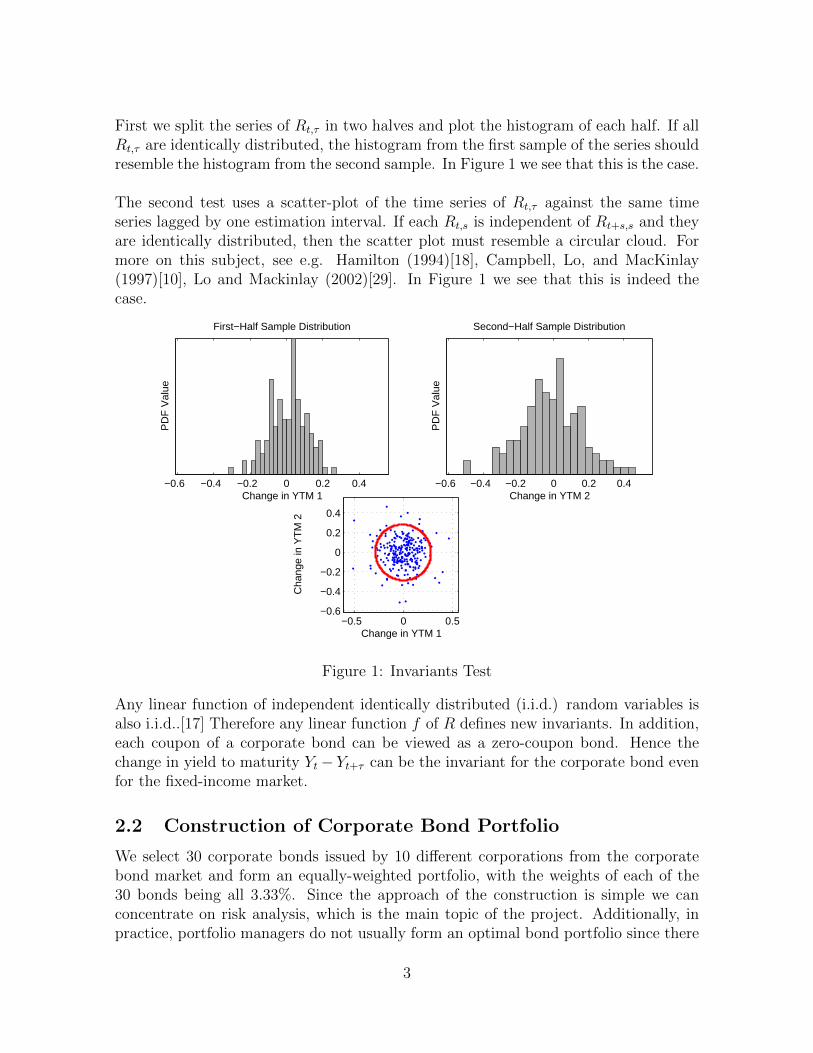
First we split the series of Rt,τ in two halves and plot the histogram of each half. If allRt,τ are identically distributed, the histogram from the first sample of the series shouldresemble the histogram from the second sample. In Figure 1 we see that this is the case.

The second test uses a scatter-plot of the time series of Rt,τ against the same timeseries lagged by one estimation interval. If each Rt,s is independent of Rt+s,s and theyare identically distributed, then the scatter plot must resemble a circular cloud. Formore on this subject, see e.g. Hamilton (1994)[18], Campbell, Lo, and MacKinlay(1997)[10], Lo and Mackinlay (2002)[29]. In Figure 1 we see that this is indeed thecase.

−0.6 −0.4 −0.2 0 0.2 0.4Change in YTM 1

PD

F V

alue

First−Half Sample Distribution

−0.6 −0.4 −0.2 0 0.2 0.4Change in YTM 2

PD

F V

alue

Second−Half Sample Distribution

−0.5 0 0.5−0.6

−0.4

−0.2

0

0.2

0.4

Change in YTM 1

Cha

nge

in Y

TM

2

Figure 1: Invariants Test

Any linear function of independent identically distributed (i.i.d.) random variables isalso i.i.d..[17] Therefore any linear function f of R defines new invariants. In addition,each coupon of a corporate bond can be viewed as a zero-coupon bond. Hence thechange in yield to maturity Yt− Yt+τ can be the invariant for the corporate bond evenfor the fixed-income market.

2.2 Construction of Corporate Bond Portfolio

We select 30 corporate bonds issued by 10 different corporations from the corporatebond market and form an equally-weighted portfolio, with the weights of each of the30 bonds being all 3.33%. Since the approach of the construction is simple we canconcentrate on risk analysis, which is the main topic of the project. Additionally, inpractice, portfolio managers do not usually form an optimal bond portfolio since there

3

are factors that need to be considered for bonds like default probabilities, recoveryrates, embedded call features, and coupon rates.[40] Forming an optimal bond portfoliois challenging.

2.3 Computation of Market VaR of the Portfolio

There are three major approaches to calculating value-at-risk; the variance-covariance(delta-normal) method, historical simulation, and Monte Carlo simulation.

2.3.1 Variance-Covariance Approach

For the variance-covariance method, we need to assume risk variables (log-return inequity market and the change in yield to maturity in the fixed-income market) followa specific distribution (usually the normal distribution). The two moments of thedistribution, mean and variance, are calculated by the formulas:

µp = WWW Tµµµa

σ2p = WWW TCCCWWW

where µp and σ2p are the mean and variance of the portfolio respectively.

WWW is a vector of weights of each bond,CCC is the covariance matrix of change in yield to maturity of different bonds in the timeseries,µµµa is a vector of the expectation of change in yield to maturity of each bond.Then we can calculate VaR with confidence level 99% by the formula[27]:

VaR99% = µp − σpNNN−1(99%) (4)

where NNN−1(99%) is 99% quantile of normal distribution NNN(µp, σ2p).

The strength of the variance-covariance approach is that VaR is simple to computeonce you have made an assumption about the distribution of risk factors and insertedthe means, variances, and covariances of risk factors; however, this approach has threelimitations. First, the normal distribution is not realistic in many cases. If risk factorsare not normally distributed, then the formula for the computation of VaR will also beaffected, otherwise it would understate the true VaR. The second limitation is inputerror. Even if the distribution assumption holds, the VaR can still be wrong if thevariances and covariances that are used to estimate it are incorrect. The last limita-tion is non-stationary variables which occurs when technically the entire distributioncan change across assets over time.

4

2.3.2 Historical Simulation Approach

Historical simulation is the simplest method of estimating the VaR for many portfo-lios. To run a historical simulation, we begin with time series data on each market riskfactor just as we do in the variance-covariance approach; however, we do not use thedata to estimate variances and covariances looking forward since the changes in theportfolio over time yield all the information we need to compute the VaR.

We form order statistics for the historical time series of risk factors and sort themin descending order. With 99% confidencel, the 99th percentile of the historical or-dered risk factor data is the VaR99%.[3]

While this approach is popular and relatively easy to run, it has some weaknesses. Forexample, historical simulation is excessively dependent on past data. If some historicaldata is lost, then there may be a substantial error in the final result. Additionally,trends in the data are ignored in historical simulation. The approach assigns the sameweight to every data point. In reality, yesterday’s events weigh more on the presentthan the past year’s events.

2.3.3 Monte Carlo Simulation Approach

The first two steps in a Monte Carlo simulation[4] are same as the variance-covarianceapproach where we identify the market risk factors and calculate the mean vectorand covariance matrix including each asset. Next we will generate sample paths ofthe risk factors. For example, we suppose the risk factor follows multivariate normaldistribution, which has the following probability density function [20]:

fxxx(x1, ..., xk) =1√

|(2π)kCCC|exp(−1

2(xxx− µµµ)TCCC−1(xxx− µµµ)). (5)

Once the distributions are specified, the simulation process can begin. In each run,the market risk variables take on different outcomes and the value of the portfolioreflects the outcomes. After a repeated series of runs, we will have a distribution ofportfolio values that can be used to assess VaR. For example, assume we run a se-ries of 1,000,000 simulations and derive corresponding values for the portfolio. Thesevalues can be ranked from highest to lowest, and the 99% VaR is the 100th lowest value.

Unlike the variance-covariance approach, Monte Carlo simulation is easily understoodand can be applied to almost all kinds of financial securities and instruments; however,it usually requires a high time-cost in terms of computation because it depends uponthe number of repeated runs.

Since the distribution of risk factors (change in yield to maturity) has a heavy fat-tailfeature, we reject the variance-covariance approach. Additionally, due to the strong

5

data dependencies and trends in data, we also reject historical simulation. Althoughthe multivariate normal distribution assumption is inapproriate for the Monte Carlosimulation, the central limit theorem (CLT)[2] and the law of large numbers[13] sup-port that Monte Carlo simulation is more accurate than the other two methods in thecomputation of VaR for fixed-income securities.[8] By using the Monte Carlo simula-tion approach we derive the VaR of the market risk component from our dataset andestimate that VaR99% =0.48%. This implies that if we invest 1,000,000 USD in ourportfolio today, then there is a 1% chance that we could lose more than 4,800 USD inthe next month.

3 Credit Risk Analysis

Corporate bond investors are exposed to credit risk because the counterparty (cor-poration) may default on its obligations. Therefore in order to measure credit riskof corporate bond portfolios, we need to consider three important factors. They aredefault probabilities, losses given default, and exposures to each asset.

In this section we will discuss approaches of computing default risk. The Mertonmodel[1] is an extension of the Black-Scholes option pricing model[6]. It estimates thevalue of the bondholders’ and stockholders’ claims, which are then used to estimate theimplied probability of default. Moody’s KMV[5] model improves the Merton model byrelaxing some of the assumptions. These two methods are fequently used in analyzingthe default probabilities of corporate bonds.

3.1 Merton Model

Before moving on to the Merton model, let us discuss the Black-Scholes option pricingformula first. The Black-Scholes model of the market for a specific stock makes thefollowing explicit assumptions:

• There are no arbitrage opportunities.

• It is possible to borrow and lend cash at a known constant risk-free interest rate.

• Short selling is allowed.

• The stock price follows a geometric Brownian motion with constant drift andvolatility.

• The underlying security does not pay a dividend.

• The financial market is frictionless.

• Fractional amounts of the underlying asset can be traded.

6

Based on these strong assumptions, we can deduce following Black-Scholes partialdifferential equation:

∂f

∂t+ rS

∂f

∂S+

1

2σ2S2 ∂

2f

∂S2= rf (6)

where f is a European style option price at time t. S is the underlying market priceat time t. r is risk-free interest rate, and it is also the drift of the geometric Brownianmotion under the risk-neutral measure. σ is the volatility of the underlying. Theanalytical solution is [37]:

c0 = S0N(d1)−Ke−rTN(d2)

p0 = Ke−rTN(−d2)− S0N(−d1)

where:

d1 =ln(S0

K) + (r + σ2

2)T

σ√T

d2 = d1 − σ√T ,

c0 is the price of the European call option with strike price K and maturity T , and p0is the price of the European put option with strike price K and maturity T .

For a corporation its asset value is equal to the sum of its liabilities and equity value.The Merton model assumes a corporation only issues one zero-coupon bond during itsbusiness cycle. Therefore the accounting formula: ‘Asset = Liability + Equity’ will betransformed into

AT = B + ST (7)

where AT is the corporation’s asset value at maturity, ST is the market capitalizationof the corporation at maturity, and B is the face value of the zero-coupon bond.Similarly we assume the asset price follows a geometric Brownian motion. At maturityT , if AT≤B, then ST will be equal to zero and the corporation faces default on itsobligation. Therefore we can rewrite the formula as:

ST = max(AT −B, 0).

This implies the market capitalization of the corporation’s equity value can be explainedas a call option on the corporation’s assets with strike price equal to the face value ofthe zero-coupon bond. Using the Black-Scholes model we can obtain the formula forS0 under the Merton model,

S0 = A0N(d1)−BerTN(d2) (8)

where

d1 =ln(A0erT

B)

σA√T

+1

2σA√T

7

d2 = d1 − σA√T ,

σA is the volatility of the asset value, and r is the risk-free rate of interest, both ofwhich are assumed to be constant.

Next we deal with the default probability. Define B0 = Be−rT as the present value ofthe future payoff of the zero-coupon bond, and let L = B0

A0be a measure of the leverage

of the corporation[24]. Plug these two parameters back into the solution of the formula(8) to obtain

S0 = A0[N(d1)− LN(d2))] (9)

where

d1 = − ln(L)

σA√T

+1

2σA√T

d2 = d1 − σA√T .

Since the equity value is a function of the asset value we can apply Ito’s lemma[25] todetermine the instantaneous volatility of the equity from the asset volatility:

S0σS =∂S

∂AA0σA (10)

where σS is the instantaneous volatility of the company’s equity at time zero. Fromformula (9) we obtain

A0

S0

=1

N(d1)− LN(d2), (11)

and from formula (8) we obtain∂S

∂A= N(d1). (12)

Therefore equations (10), (11) and (12) lead to

σS =σAN(d1)

N(d1)− LN(d2). (13)

Equations (9) and (13) allow A0 and σA to be obtained from observed S0, L, and Tand the statistical estimate σS. The risk-neutral probability that the corporation willdefault at the maturity T is the probability that shareholders will not exercise theircall option to buy the assets of the company for value B at the maturity time T . Theprobability is given by [34]

P = 1−N(d2). (14)

The Merton model is simple to understand and easy to implement. It makes sense fornon-mathematicians to use market data such as stock values and capital structure topredict the probability of default. While this is applicable, it also has some problems

8

due to its unrealistic assumptions. For example, if there is only one issue of equityand debt, and if the debt is in the form of a zero-coupon bond that matures at agiven date, then default can only occur at the maturity date. The value of the firmis observable and follows a lognormal diffusion process (geometric Brownian motion).There is no negotiation between shareholders and debtholders, there is no need toadjust for liquidity, and the risk-free interest rate is constant.

3.2 Moody’s KMV model

The KMV model is built on the Merton model and tries to improve some of its short-comings. The most notable change is that it relaxes the assumption that all the debtmature at the same time. The KMV model divides the debt of a corporation into short-term liabilities and long-term liabilities which have different maturities. We combinethese two values together to determine the default point. A practical rule for thedetermination of the default threshold[14] is:

B = SL+1

2LL (15)

where SL stands for the short-term liabilities, LL refers to the long-term liabilities,and B is default threshold.

In the Merton model, we know there are three elements that determine the defaultprobability of a firm: the value of company’s assets, the uncertainty of the assets (i.e.volatility of the assets), and leverage.

There are six variables that determine the default probability of a firm over somehorizon, from the current time until H (see Figure 2)

Figure 2: KMV model (Source: Crosbie and Bohn, 2004)

9

In the Figure 2 above,[12] 1© is the current asset value. 2© is the distribution of theasset value at time H. 3© is the volatility of the future assets value at time H. 4© is thelevel of the default point. 5© is the expected rate of growth in the asset value over thehorizon. 6© is the length of the horizon, H.

If the value of the assets falls below the default point, then the firm defaults. Thereforethe probability of default is the probability that the asset value will fall below the de-fault point. This is depicted by the shaded area (Expected Default Frequency) belowthe default point in Figure 2.

There are essentially three steps in the computation of the default probability of afirm. First, estimate the asset value and the volatility from the formulas (9) and (13).We can observe market capitalization of the company which is the product of the stockprice and the number of outstanding shares and then derive the σS by estimating thevariance of the market value of the company. Second, KMV measures the distance-to-default as the number of standard deviations the asset value is away from default,and then uses empirical data to determine the corresponding default probability. Thedistance-to-default is calculated (DD) as

DD =E(A)−B

σA(16)

where E(A) refers to expected value of the asset and B is the default threshold.

From formula (16) we learn that DD is the number of standard deviations away fromthe default threshold B. Lastly after we obtain the DD we compare it to our his-torical database to find the corresponding DD in the historical default distribution.The KMV model needs a database that includes over 250,000 company-years of dataand over 4,700 incidents of default or bankruptcy. From this data a lookup or fre-quency table can be generated which relates the likelihood of default to various levelsof distance-to-default.[32]

For example, assume that we are interested in determining the default probabilityover the next year for a firm that is 7 standard deviations away from default. To deter-mine this expected default frequency (EDF) value, we query the default history for theproportion of the firms. Seven standard deviations away from default that defaultedover the next year. The answer is about 5 basis points(bp), 0.05%, or an equivalentcredit rating of AA according to Moody’s.[38]

In order to estimate the default risk of the corporate bond portfolio under the KMVmodel, we require some fundamental data for the corporation like short-term and long-term liabilities and outstanding shares. The shortest period of financial statementissuing is quarterly and this project is focused on risk analysis in a 1-month investment

10

horizon. Hence we only illustrate the idea of the KMV model in the report rather thanpresenting the implementation process.

3.3 Calculation of Credit VaR of the Portfolio

The expected loss is equal to the product of the default probability, loss given default,and particular bond exposure,

LtLtLt = W TW TW TP tdPtdPtdLGDLGDLGD (17)

where WWW is the weight of each asset in the portfolio, P tdPtdPtd is vector containing default

probabilities of every asset at time t, LGDLGDLGD is a vector of loss given the default of eachbond (we assume all bonds have a recovery rate of 30% over the bonds’ life, whichmeans loss given default is 70%). Therefore LtLtLt is the vector of the expected loss drivenby credit risk at time t.

Based on formulas (9), (13), and (14), we can generate a matrix of default proba-bilities which contains time series of default probabilities of each bond. Then by usingformula (17), we can derive a time series of the expected loss of each bond.

In order to simplify the computation, we assume the default risks are linearly cor-related. Then we use Monte Carlo simulation to generate the expected loss of theportfolio in one month. Next we select the 99th percentile of the simulation value tobe the credit VaR with a 99% confidence level.[26] The result is VaR99% = 4%. Thismeans that if we invest 1,000,000 USD in our portfolio today, there is a 1% chancethat we could lose more than 40,000 USD next month.

4 Liquidity Risk Analysis

4.1 Definition of Basis

Quantifying liquidity risk is the hardest part of risk analysis because it is difficult tofind a parameter that represents the liquidity features of a corporate bond.

We have already discussed that a corporate bond is exposed to three main risks whichare market risk, credit risk, and liquidity risk. In order to bear these three risks, aninvestor requires a specified yield from the corporate bond. We know that a major partof market risk is driven by the fluctuation of the interest rate. We could say that thebond yield spread (i.e. the difference between the bond yield and the risk-free interest)is the return we require to bear both the credit risk and the liquidity risk. In many fi-nancial markets there is an instrument called the credit default swap (CDS) which wasinvented by Blythe Masters from JP Morgan in 1994. “A credit default swap (CDS) isa financial swap agreement that the seller of the CDS will compensate the buyer in the

11

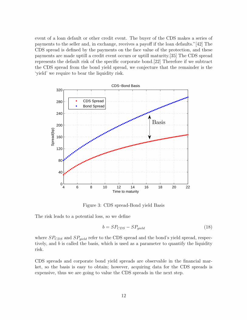
event of a loan default or other credit event. The buyer of the CDS makes a series ofpayments to the seller and, in exchange, receives a payoff if the loan defaults.”[42] TheCDS spread is defined by the payments on the face value of the protection, and thesepayments are made uptill a credit event occurs or uptill maturity.[35] The CDS spreadrepresents the default risk of the specific corporate bond.[22] Therefore if we subtractthe CDS spread from the bond yield spread, we conjecture that the remainder is the‘yield’ we require to bear the liquidity risk.

4 6 8 10 12 14 16 18 20 220

40

80

120

160

200

240

280

320

Time to maturity

Spr

ead(

bp)

CDS−Bond Basis

CDS SpreadBond Spread

Basis

Figure 3: CDS spread-Bond yield Basis

The risk leads to a potential loss, so we define

b = SPCDS − SPyield (18)

where SPCDS and SPyield refer to the CDS spread and the bond’s yield spread, respec-tively, and b is called the basis, which is used as a parameter to quantify the liquidityrisk.

CDS spreads and corporate bond yield spreads are observable in the financial mar-ket, so the basis is easy to obtain; however, acquiring data for the CDS spreads isexpensive, thus we are going to value the CDS spreads in the next step.

12

4.2 Valuation of Credit Default Swap Spread

A credit default swap (CDS) is the most popular form of protection against default.The goal of CDS valuation is to determine the value of the mid-market (i.e., averageof bid and ask prices) CDS spread on the reference entity, which is the company uponwhich default protection is bought and sold. There are four steps to calculating theCDS spread[23]:

Step 1: Calculate the present value of expected payments. Payments are made atthe CDS spread rate, s, and multiplied by the reference entity’s probability of survivaleach year. The sum of the present value of each annual payment equals the presentvalue of expected payments.

Step 2: Calculate the present value of the expected payoff in the event of default.To make this calculation, we first need to make an assumption about when defaultsoccur. It is common to assume that defaults occur halfway through a year. This isbecause almost all the corporate bonds pay coupons biannually. If the corporationcannot pay the coupon, then we can claim that it defaulted on its obligation. Theassumptions make sense from a practical perspective. From these assumptions theannual default probability is multiplied by the reference entity’s loss given default anddiscounted back to the present.

Step 3: Calculate the present value of the accrual payment in the event of default.Since payments are made in arrears, an accrual payment is required in the event ofdefault to account for the time between the beginning of the year and the time whendefault actually occurs. If we assume that defaults occur halfway through the year, theaccrual payment will be 1

2s. The annual accrual payment is multiplied by the proba-

bility of default each year and discounted to the present.

Step 4: Calculate the CDS spread. Solve for s by equating the expected presentvalue of total payments to the expected present value of payoff in the event of default.

From the above steps, we can derive the following formula:

s =PV (payoff)

PV (payments)(19)

where PVpayoff means the present value of the expected payoff in the event of defaultand PVpayments means the present value of the sum of expected payments made at theCDS spread rate, s, and accrual payments in the event of default.

It is also assumed that each CDS has the same maturity as the corresponding cor-porate bond and that the default probabilities and recovery rates remain constant.Based on these assumptions we can predict both the future payoff and the total ex-

13

pected payments (the sum of payments made at the CDS spread rate and accrualpayment in the event of default).

We use this approach to approximate the CDS spread upon these 30 reference bonds.We have already estimated probability of default in each month, therefore we cangenerate a time series of CDS spreads for each reference bond.

4.3 Estimation of Liquidity VaR of the Portfolio

We have already defined a parameter called basis which is the difference between theCDS spread and its reference bond’s yield spread. Usually the CDS spread is less thanthe bond yield spread. Thus the basis is a negative value. As we have already discussedabove, the remainder of subtracting the CDS spread from the reference bond’s yieldspread is the investor’s required return to bear the liquidity risk. So the followingformula shows a potential loss of the portfolio because of the liquidity risk,

Lliq = W TW TW Tbbb (20)

where Lliq is the loss of the portfolio derived from liquidity risk, WWW is the vector ofweights of each bond, and bbb is the vector of basis of each bond.

Formula (16) helps us estimate the basis of every bond at the beginning of each month.Thus we can obtain a time series for the basis. Next we estimate the mean and covari-ance of the estimated historical basis and apply the multivariate normal distributionassumption to run Monte Carlo simulations to calculate the liquidity VaR with 99%confidence one month later. The result is VaR99% = 5.73%. This means that if weinvest 1,000,000 USD in our portfolio today, there is a 1% chance that we could losemore than 57,300 USD next month.

5 Common Risk Factors in the Returns on Bonds

This section identifies five common risk factors in the returns on bonds; three factorsof which come from the stock market. Stock returns have shared variation due to thestock-market factors and they are linked to bond returns through shared variation inthe bond-market factors. Except for low-grade corporate bonds, the bond-market fac-tors capture the common variation in bond returns.

When considering stock and bond returns, one famous approach is called the Fama-French common risk factors model[15]. In this report we are going to test our bondportfolio by using these common factors. Intuitively if we assume that the financialmarket is an integrated market (i.e. financial securities’ prices among different loca-tions or related goods follow similar patterns over a long period), we seek some commonfactors that affect both stocks’ and bonds’ average returns.

14

The list of empirical factors that we may consider contains securities’ systematic riskβ, issue size, leverage of stocks or bonds, book-to-market ratio, TERM , and DEF .The followings are these factors’ definitions and considerations in our report.

5.1 Introduction to Fama-French Factors

First of all, let us consider some common factors that might be related to stock ex-pected average returns.

The first one is the systematic risk β, which is derived from the Capital Asset PricingModel (CAPM).[36] Under CAPM we have

E(Ri) = Rf + βi(E(Rm − r)), (21)

where Rm is the market expected return, and r is the risk-free return. The marketrisk β represents how risky one financial security is. If β>1, we conclude that thissecurity is more risky than the market and is less risky than the market otherwise.Based on Fama and French’s research, the cross-section of average returns on U.S.common stocks shows little relation with this β. In this report we ignore this factor inour regression model.

Issue size, intuitively speaking, is related to one security’s profitability. The biggerthe issue size, the more liquid the security, and the less the bid-ask spread would be.In this sense investors prefer to invest in these bonds associated with large size issue,and large size issue could result in a negative relationship with average return. In thebusiness world the small firms usually would get lower credit ratings, and they usuallydo not issue bonds as large as some big companies. The size effect would be moreobvious during some specific periods. We use the issue size as the first common factor.The size is considered as following:

Size = SN (22)

where S is stock market price and N is numbers of outstanding shares in the market.

The leverage factor is another important factor in this paper. Typically the higherthe leverage of one security, the higher the expected return would be. The reasonis quite simple, higher return would be associated with higher risk. For stocks theleverage is defined as[7]

Leverage =Earnings

Price. (23)

Since the market is efficient under our assumption, the leverage factor is considerednot only for stocks but also for bonds.

15

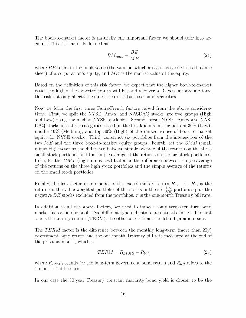
The book-to-market factor is naturally one important factor we should take into ac-count. This risk factor is defined as

BMratio =BE

ME(24)

where BE refers to the book value (the value at which an asset is carried on a balancesheet) of a corporation’s equity, and ME is the market value of the equity.

Based on the definition of this risk factor, we expect that the higher book-to-marketratio, the higher the expected return will be, and vice versa. Given our assumptions,this risk not only affects the stock securities but also bond securities.

Now we form the first three Fama-French factors raised from the above considera-tions. First, we split the NYSE, Amex, and NASDAQ stocks into two groups (Highand Low) using the median NYSE stock size. Second, break NYSE, Amex and NAS-DAQ stocks into three categories based on the breakpoints for the bottom 30% (Low),middle 40% (Medium), and top 30% (High) of the ranked values of book-to-marketequity for NYSE stocks. Third, construct six portfolios from the intersection of thetwo ME and the three book-to-market equity groups. Fourth, set the SMB (smallminus big) factor as the difference between simple average of the returns on the threesmall stock portfolios and the simple average of the returns on the big stock portfolios.Fifth, let the HML (high minus low) factor be the difference between simple averageof the returns on the three high stock portfolios and the simple average of the returnson the small stock portfolios.

Finally, the last factor in our paper is the excess market return Rm − r. Rm is thereturn on the value-weighted portfolio of the stocks in the six BE

MEportfolios plus the

negative BE stocks excluded from the portfolios. r is the one-month Treasury bill rate.

In addition to all the above factors, we need to impose some term-structure bondmarket factors in our pool. Two different type indicators are natural choices. The firstone is the term premium (TERM), the other one is from the default premium side.

The TERM factor is the difference between the monthly long-term (more than 20y)government bond return and the one month Treasury bill rate measured at the end ofthe previous month, which is

TERM = RLTMG −Rbill (25)

where RLTMG stands for the long-term government bond return and Rbill refers to the1-month T-bill return.

In our case the 30-year Treasury constant maturity bond yield is chosen to be the

16

long-term government bond return. This risk factor should capture the risk premiumthat arises from an unexpected interest rate change. Especially for the bond market,the interest rate risk (duration risk) is one main risk source. We would use the sampledata set to test this factor and try to quantify the term premium as accurately aspossible.

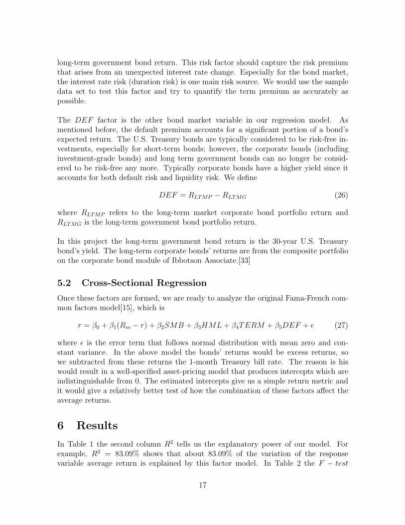
The DEF factor is the other bond market variable in our regression model. Asmentioned before, the default premium accounts for a significant portion of a bond’sexpected return. The U.S. Treasury bonds are typically considered to be risk-free in-vestments, especially for short-term bonds; however, the corporate bonds (includinginvestment-grade bonds) and long term government bonds can no longer be consid-ered to be risk-free any more. Typically corporate bonds have a higher yield since itaccounts for both default risk and liquidity risk. We define

DEF = RLTMP −RLTMG (26)

where RLTMP refers to the long-term market corporate bond portfolio return andRLTMG is the long-term government bond portfolio return.

In this project the long-term government bond return is the 30-year U.S. Treasurybond’s yield. The long-term corporate bonds’ returns are from the composite portfolioon the corporate bond module of Ibbotson Associate.[33]

5.2 Cross-Sectional Regression

Once these factors are formed, we are ready to analyze the original Fama-French com-mon factors model[15], which is

r = β0 + β1(Rm − r) + β2SMB + β3HML+ β4TERM + β5DEF + ε (27)

where ε is the error term that follows normal distribution with mean zero and con-stant variance. In the above model the bonds’ returns would be excess returns, sowe subtracted from these returns the 1-month Treasury bill rate. The reason is hiswould result in a well-specified asset-pricing model that produces intercepts which areindistinguishable from 0. The estimated intercepts give us a simple return metric andit would give a relatively better test of how the combination of these factors affect theaverage returns.

6 Results

In Table 1 the second column R2 tells us the explanatory power of our model. Forexample, R2 = 83.09% shows that about 83.09% of the variation of the responsevariable average return is explained by this factor model. In Table 2 the F − test

17

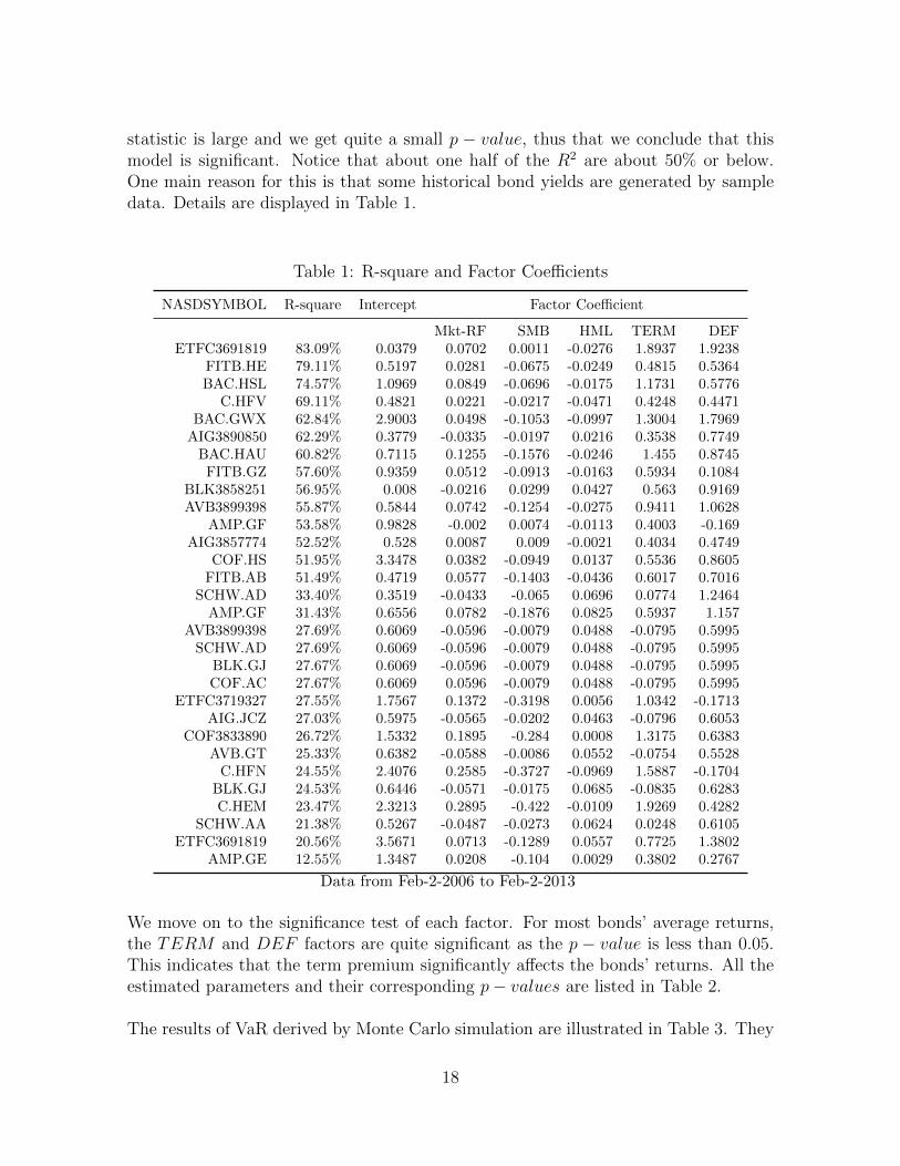
statistic is large and we get quite a small p − value, thus that we conclude that thismodel is significant. Notice that about one half of the R2 are about 50% or below.One main reason for this is that some historical bond yields are generated by sampledata. Details are displayed in Table 1.

Table 1: R-square and Factor Coefficients

NASDSYMBOL R-square Intercept Factor Coefficient

Mkt-RF SMB HML TERM DEFETFC3691819 83.09% 0.0379 0.0702 0.0011 -0.0276 1.8937 1.9238

FITB.HE 79.11% 0.5197 0.0281 -0.0675 -0.0249 0.4815 0.5364BAC.HSL 74.57% 1.0969 0.0849 -0.0696 -0.0175 1.1731 0.5776

C.HFV 69.11% 0.4821 0.0221 -0.0217 -0.0471 0.4248 0.4471BAC.GWX 62.84% 2.9003 0.0498 -0.1053 -0.0997 1.3004 1.7969

AIG3890850 62.29% 0.3779 -0.0335 -0.0197 0.0216 0.3538 0.7749BAC.HAU 60.82% 0.7115 0.1255 -0.1576 -0.0246 1.455 0.8745FITB.GZ 57.60% 0.9359 0.0512 -0.0913 -0.0163 0.5934 0.1084

BLK3858251 56.95% 0.008 -0.0216 0.0299 0.0427 0.563 0.9169AVB3899398 55.87% 0.5844 0.0742 -0.1254 -0.0275 0.9411 1.0628

AMP.GF 53.58% 0.9828 -0.002 0.0074 -0.0113 0.4003 -0.169AIG3857774 52.52% 0.528 0.0087 0.009 -0.0021 0.4034 0.4749

COF.HS 51.95% 3.3478 0.0382 -0.0949 0.0137 0.5536 0.8605FITB.AB 51.49% 0.4719 0.0577 -0.1403 -0.0436 0.6017 0.7016

SCHW.AD 33.40% 0.3519 -0.0433 -0.065 0.0696 0.0774 1.2464AMP.GF 31.43% 0.6556 0.0782 -0.1876 0.0825 0.5937 1.157

AVB3899398 27.69% 0.6069 -0.0596 -0.0079 0.0488 -0.0795 0.5995SCHW.AD 27.69% 0.6069 -0.0596 -0.0079 0.0488 -0.0795 0.5995

BLK.GJ 27.67% 0.6069 -0.0596 -0.0079 0.0488 -0.0795 0.5995COF.AC 27.67% 0.6069 0.0596 -0.0079 0.0488 -0.0795 0.5995

ETFC3719327 27.55% 1.7567 0.1372 -0.3198 0.0056 1.0342 -0.1713AIG.JCZ 27.03% 0.5975 -0.0565 -0.0202 0.0463 -0.0796 0.6053

COF3833890 26.72% 1.5332 0.1895 -0.284 0.0008 1.3175 0.6383AVB.GT 25.33% 0.6382 -0.0588 -0.0086 0.0552 -0.0754 0.5528

C.HFN 24.55% 2.4076 0.2585 -0.3727 -0.0969 1.5887 -0.1704BLK.GJ 24.53% 0.6446 -0.0571 -0.0175 0.0685 -0.0835 0.6283C.HEM 23.47% 2.3213 0.2895 -0.422 -0.0109 1.9269 0.4282

SCHW.AA 21.38% 0.5267 -0.0487 -0.0273 0.0624 0.0248 0.6105ETFC3691819 20.56% 3.5671 0.0713 -0.1289 0.0557 0.7725 1.3802

AMP.GE 12.55% 1.3487 0.0208 -0.104 0.0029 0.3802 0.2767

Data from Feb-2-2006 to Feb-2-2013

We move on to the significance test of each factor. For most bonds’ average returns,the TERM and DEF factors are quite significant as the p − value is less than 0.05.This indicates that the term premium significantly affects the bonds’ returns. All theestimated parameters and their corresponding p− values are listed in Table 2.

The results of VaR derived by Monte Carlo simulation are illustrated in Table 3. They

18

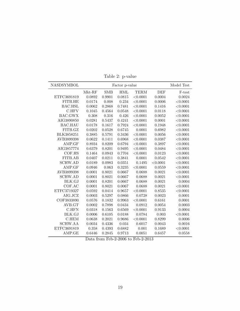
Table 2: p-value

NASDSYMBOL Factor p-value Model Test

Mkt-RF SMB HML TERM DEF F-testETFC3691819 0.0892 0.9901 0.0815 <0.0001 0.0004 0.0024

FITB.HE 0.0174 0.008 0.234 <0.0001 0.0006 <0.0001BAC.HSL 0.0062 0.2868 0.7481 <0.0001 0.1416 <0.0001

C.HFV 0.1045 0.4564 0.0548 <0.0001 0.0118 <0.0001BAC.GWX 0.308 0.316 0.426 <0.0001 0.0052 <0.0001

AIG3890850 0.0281 0.5437 0.4241 <0.0001 0.0001 <0.0001BAC.HAU 0.0178 0.1617 0.7924 <0.0001 0.1948 <0.0001FITB.GZ 0.0202 0.0528 0.6745 0.0001 0.6982 <0.0001

BLK3858251 0.3885 0.5791 0.3436 <0.0001 0.0056 <0.0001AVB3899398 0.0622 0.1411 0.6968 <0.0001 0.0387 <0.0001

AMP.GF 0.8934 0.8209 0.6794 <0.0001 0.3897 <0.0001AIG3857774 0.6379 0.8201 0.9495 <0.0001 0.0484 <0.0001

COF.HS 0.1464 0.0943 0.7704 <0.0001 0.0123 <0.0001FITB.AB 0.0407 0.0211 0.3841 0.0001 0.0542 <0.0001

SCHW.AD 0.0189 0.0983 0.0351 0.1495 <0.0001 <0.0001AMP.GF 0.0946 0.063 0.3235 <0.0001 0.0559 <0.0001

AVB3899398 0.0001 0.8021 0.0667 0.0688 0.0021 <0.0001SCHW.AD 0.0001 0.8021 0.0667 0.0688 0.0021 <0.0001

BLK.GJ 0.0001 0.8201 0.0667 0.0688 0.0021 0.0004COF.AC 0.0001 0.8021 0.0067 0.0688 0.0021 <0.0001

ETFC3719327 0.0592 0.0414 0.9657 <0.0001 0.8535 <0.0001AIG.JCZ 0.0003 0.5297 0.0866 0.0728 0.0023 0.0001

COF3833890 0.0576 0.1832 0.9963 <0.0001 0.6161 0.0001AVB.GT 0.0002 0.7898 0.0434 0.0912 0.0054 0.0003

C.HFN 0.0318 0.1563 0.6569 <0.0001 0.9133 0.0004BLK.GJ 0.0006 0.6105 0.0188 0.0784 0.003 <0.0001C.HEM 0.0638 0.2021 0.9686 <0.0001 0.8299 0.0006

SCHW.AA 0.0034 0.4336 0.034 0.6017 0.0043 0.0016ETFC3691819 0.358 0.4393 0.6882 0.001 0.1689 <0.0001

AMP.GE 0.6446 0.2845 0.9713 0.0051 0.6457 0.0558

Data from Feb-2-2006 to Feb-2-2013

19

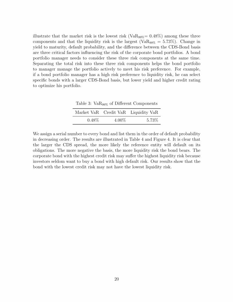
illustrate that the market risk is the lowest risk (VaR99%= 0.48%) among these threecomponents and that the liquidity risk is the largest (VaR99% = 5.73%). Change inyield to maturity, default probability, and the difference between the CDS-Bond basisare three critical factors influencing the risk of the corporate bond portfolios. A bondportfolio manager needs to consider these three risk components at the same time.Separating the total risk into these three risk components helps the bond portfolioto manager manage the portfolio actively to meet his risk preference. For example,if a bond portfolio manager has a high risk preference to liquidity risk, he can selectspecific bonds with a larger CDS-Bond basis, but lower yield and higher credit ratingto optimize his portfolio.

Table 3: VaR99% of Different Components

Market VaR Credit VaR Liquidity VaR

0.48% 4.00% 5.73%

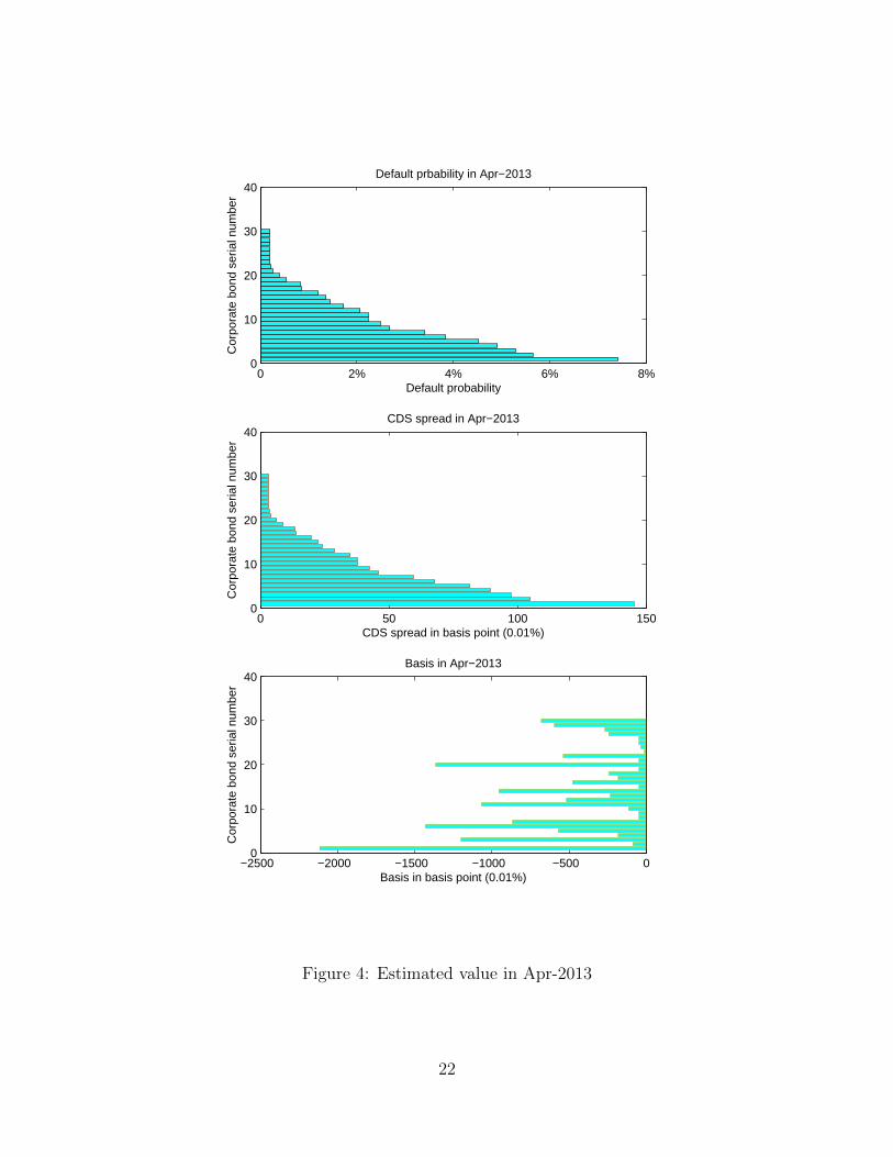
We assign a serial number to every bond and list them in the order of default probabilityin decreasing order. The results are illustrated in Table 4 and Figure 4. It is clear thatthe larger the CDS spread, the more likely the reference entity will default on itsobligations. The more negative the basis, the more liquidity risk the bond bears. Thecorporate bond with the highest credit risk may suffer the highest liquidity risk becauseinvestors seldom want to buy a bond with high default risk. Our results show that thebond with the lowest credit risk may not have the lowest liquidity risk.

20

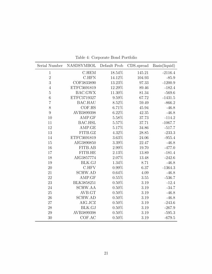
Table 4: Corporate Bond Portfolio

Serial Number NASDSYMBOL Default Prob CDS spread Basis(liquid)

1 C.HEM 18.54% 145.21 -2116.42 C.HFN 14.12% 104.93 -85.93 COF3833890 13.23% 97.33 -1200.94 ETFC3691819 12.29% 89.46 -182.45 BAC.GWX 11.30% 81.34 -569.66 ETFC3719327 9.59% 67.72 -1431.57 BAC.HAU 8.52% 59.49 -866.28 COF.HS 6.71% 45.94 -46.89 AVB3899398 6.22% 42.35 -46.810 AMP.GF 5.58% 37.73 -114.211 BAC.HSL 5.57% 37.71 -1067.712 AMP.GE 5.17% 34.86 -517.713 FITB.GZ 4.32% 28.85 -233.314 ETFC3691819 3.63% 24.06 -955.415 AIG3890850 3.39% 22.47 -46.816 FITB.AB 2.99% 19.70 -477.017 FITB.HE 2.13% 13.89 -181.418 AIG3857774 2.07% 13.48 -242.619 BLK.GJ 1.34% 8.71 -46.820 C.HFV 0.99% 6.37 -1364.321 SCHW.AD 0.64% 4.09 -46.822 AMP.GF 0.55% 3.55 -536.723 BLK3858251 0.50% 3.19 -12.424 SCHW.AA 0.50% 3.19 -34.725 AVB.GT 0.50% 3.19 -46.826 SCHW.AD 0.50% 3.19 -46.827 AIG.JCZ 0.50% 3.19 -243.628 BLK.GJ 0.50% 3.19 -267.929 AVB3899398 0.50% 3.19 -595.330 COF.AC 0.50% 3.19 -679.5

21

0 2% 4% 6% 8%0

10

20

30

40

Default probability

Cor

pora

te b

ond

seria

l num

ber

Default prbability in Apr−2013

0 50 100 1500

10

20

30

40

CDS spread in basis point (0.01%)

Cor

pora

te b

ond

seria

l num

ber

CDS spread in Apr−2013

−2500 −2000 −1500 −1000 −500 00

10

20

30

40

Basis in basis point (0.01%)

Cor

pora

te b

ond

seria

l num

ber

Basis in Apr−2013

Figure 4: Estimated value in Apr-2013

22

7 Conclusion

In summary we quantify three different types of risk: market risk, credit risk andliquidity risk. The results are derived from the sample data using the Monte Carlosimulation method. The results are displayed in Table 3.

The first important risk in a bond portfolio is the market risk, which contains in-terest rate risk. If the interest rate changes, the value of the portfolio could have asignificant fluctuation. According to duration and convexity approximation, which es-sentially tells us how much percentage change our bond portfolio value will experience,a bond portfolio manager can quantify its market risk.

Another risk that a bond portfolio manager faces is credit risk. The Merton model isused in this project to quantify credit risk. In the Merton model we consider the firm’sequity as one European call option on the assets of the company with maturity T anda strike price B which is the face value of the debt.

The third risk is liquidity risk, which is quantified by the basis defined by the dif-ference of the CDS spread and the bond yield spread. As we have discussed in thesection 4.1, the CDS spread is considered as a protection against credit risk. Subtract-ing the CDS spread from the bond yield spread can capture the liquidity feature of thebond.

In addition, we use some common financial factors to capture the bond expected re-turn. Basically the most important factors are related to size and the book-to-marketequity ratio. These five factors provide a good description of the cross-section of theaverage returns, but they do not require that we have identified the true factors. Asthese factors capture the cross-section of average returns, they can be used to guideportfolio selection. The regression parameter estimates and the historical average pre-miums for the factors can be used to estimate the expected return of the portfolio. Inpractice for a specific firm’s bond, we have to consider the sampling error seriously.Therefore we conclude that the TERM and DEF bond market factors would signif-icantly affect the bond returns at typical significance levels compared with the threeother factors. Finally we check the model assumptions (i.e. error normality), whichmake our regression model results more reasonable.

8 Further Work

In the risk analysis portion of this report, Monte Carlo simulation is used to approx-imate the three risks. The major limitation of the Monte Carlo simulation approachis its model risk. Use of different distributions would result in quite different results.Minimization of the error in the approximation is the most important concern. In

23

addition the Merton model has some unrealistic assumptions. Relaxation of some ofthe assumptions is also a further research topic.

In our regression model there are some open questions. For example, for some caseswith low R2, some other common factors should be considered to improve the model’sexplanatory power. Also if we find new factors, do they improve the adjusted-R2 anddo they have a overfitting problem? All of these and other interesting questions areleft to our future work.

24

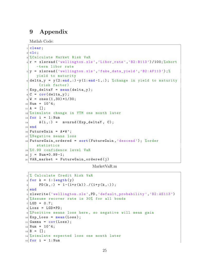
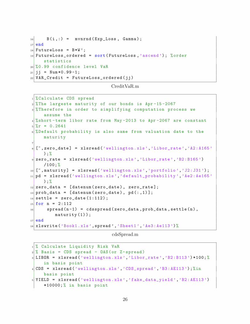
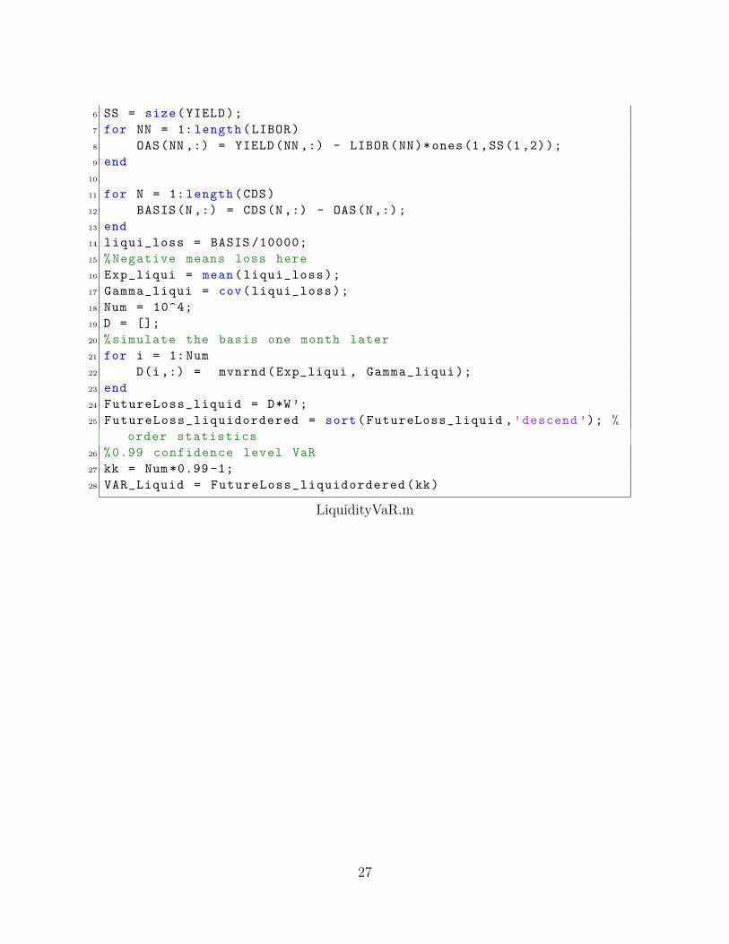
9 Appendix

Matlab Code:

1 clear;

2 clc;

3 %Calculate Market Risk VaR

4 r = xlsread(’wellington.xls’,’Libor_rate ’,’B2:B113’)/100;%short

-term libor rate

5 y = xlsread(’wellington.xls’,’fake_data_yield ’,’B2:AF113 ’);%

yield to maturity

6 delta_y = y(2:end ,:)-y(1:end -1,:); %change in yield to maturity

(risk factor)

7 Exp_deltaY = mean(delta_y);

8 C = cov(delta_y);

9 W = ones (1,30) *1/30;

10 Num = 10^4;

11 A = [];

12 %simulate change in YTM one month later

13 for i = 1:Num

14 A(i,:) = mvnrnd(Exp_deltaY , C);

15 end

16 FutureGain = A*W’;

17 %Negative means loss

18 FutureGain_ordered = sort(FutureGain ,’descend ’); %order

statistics

19 %0.99 confidence level VaR

20 j = Num *0.99 -1;

21 VAR_market = FutureGain_ordered(j)

MarketVaR.m

1 % Calculate Credit Risk VaR

2 for k = 1: length(y)

3 PD(k,:) = 1-(1+r(k))./(1+y(k,:));

4 end

5 xlswrite(’wellington.xls’,PD,’default_probability ’,’B2:AE113 ’)

6 %Assume recover rate is 30% for all bonds

7 LGD = 0.7;

8 Loss = LGD*PD;

9 %Positive means loss here , so negative will mean gain

10 Exp_Loss = mean(Loss);

11 Gamma = cov(Loss);

12 Num = 10^4;

13 B = [];

14 %simulate expected loss one month later

15 for i = 1:Num

25

16 B(i,:) = mvnrnd(Exp_Loss , Gamma);

17 end

18 FutureLoss = B*W’;

19 FutureLoss_ordered = sort(FutureLoss ,’ascend ’); %order

statistics

20 %0.99 confidence level VaR

21 jj = Num *0.99 -1;

22 VAR_Credit = FutureLoss_ordered(jj)

CreditVaR.m

1 %Calculate CDS spread

2 %The largeste maturity of our bonds is Apr -15 -2067

3 %Therefore in order to simplifying computation process we

assume the

4 %short -term libor rate from May -2013 to Apr -2067 are constant

5 %r = 0.2641

6 %Default probability is also same from valuation date to the

maturity

7

8 [~, zero_date] = xlsread(’wellington.xls’,’Libor_rate ’,’A2:A165’

);%

9 zero_rate = xlsread(’wellington.xls’,’Libor_rate ’,’B2:B165’)

/100;%

10 [~,maturity] = xlsread(’wellington.xls’,’portfolio ’,’J2:J31’);

11 pd = xlsread(’wellington.xls’,’default_probability ’,’Ae2:Ae165’

);%

12 zero_data = [datenum(zero_date), zero_rate ];

13 prob_data = [datenum(zero_date), pd(:,1)];

14 settle = zero_date (1:112);

15 for n = 2:112

16 spread(n-1) = cdsspread(zero_data ,prob_data ,settle(n),

maturity (1));

17 end

18 xlswrite(’Book1.xls’,spread ’,’Sheet1 ’,’Ae3:Ae113 ’)%

cdsSpread.m

1 % Calculate Liquidity Risk VaR

2 % Basis = CDS spread - OAS(or Z-spread)

3 LIBOR = xlsread(’wellington.xls’,’Libor_rate ’,’B2:B113’)*100;%

in basis point

4 CDS = xlsread(’wellington.xls’,’CDS_spread ’,’B3:AE113’);%in

basis point

5 YIELD = xlsread(’wellington.xls’,’fake_data_yield ’,’B2:AE113 ’)

*10000;% in basis point

26

6 SS = size(YIELD);

7 for NN = 1: length(LIBOR)

8 OAS(NN ,:) = YIELD(NN ,:) - LIBOR(NN)*ones(1,SS(1,2));

9 end

10

11 for N = 1: length(CDS)

12 BASIS(N,:) = CDS(N,:) - OAS(N,:);

13 end

14 liqui_loss = BASIS /10000;

15 %Negative means loss here

16 Exp_liqui = mean(liqui_loss);

17 Gamma_liqui = cov(liqui_loss);

18 Num = 10^4;

19 D = [];

20 %simulate the basis one month later

21 for i = 1:Num

22 D(i,:) = mvnrnd(Exp_liqui , Gamma_liqui);

23 end

24 FutureLoss_liquid = D*W’;

25 FutureLoss_liquidordered = sort(FutureLoss_liquid ,’descend ’); %

order statistics

26 %0.99 confidence level VaR

27 kk = Num *0.99 -1;

28 VAR_Liquid = FutureLoss_liquidordered(kk)

LiquidityVaR.m

27

References

[1] An Intertemporal Capital Asset Pricing Model Econometrica, Vol. 41, No.5.(Sep.,1973), pp. 867-887.

[2] Bauer, Heinz (2001) Measure and Integration Theory ISBN 3110167190.

[3] Barone-Adesi, G. and Giannopoulos, K., Vosper, L. (1999) VaR Without Correla-tions for Portfolios of Derivatives Securities Journal of Futures Markets 19: 583-602.

[4] Berry, Romain An Overview of Value-at-Risk: Part III - Monte Carlo SimulationsVaR J.P. Morgan Investment Analytics and Consulting.

[5] Bharath, Sreedhar. T and Shumway, Tyler Forecasting Default with the KMV-Merton Model University of Michigan, 12-17-2004.

[6] Black, Fischer and Scholes, Myron The Pricing of Options and Corporate LiabilitiesThe Journal of Political Economy, Vol. 81, No. 3 (May - Jun., 1973), pp. 637-654.

[7] Brigham, Eugene F. Fundamentals of Financial Management (1995).

[8] Brigo, Damiano and Mercurio, Fabio(2001) Interest Rate Models: Theory and Prac-tice with Smile, Inflation and Credit (2nd ed. 2006 ed.) Springer Verlag. ISBN978-3-540-22149-4.

[9] Brooks, Robert and Yan, Yong David London Inter-Bank Offer Rate(LIBOR)versus Treasury Rate Evidence from the Parsimonious Term Structure ModelThe Journal of Fixed Income June 1999, Vol. 9, No. 1: pp. 71-83 DOI:10.3905/jfi.1999.319232.

[10] Campbell, John Y., Lo, Andrew W. and Mackinlay, Craig The Econometrics ofFinancial Markets ISBN: 9780691043012

[11] Cooper, William H. The Russian Financial Crisis of 1998: An Analysis of Trends,Causes, and Implications Report for Congress, Feb-18-1999.

[12] Crosbit, Peter J. and Bohn, Jeffrey R. Modeling Default Risk KMV LLC ReleaseDate: 15-11-1993. Revised Date: 14-1-2002.

[13] Durrett, Richard (1995) : Probability: Theory and Examples, 2nd Edition.

[14] Fabozzi, Frank J. CFA Encyclopedia of Financial Models, 3 Volume Set.

[15] Fama, Eugene F. and French, Kenneth R. Common risk factors in the returns onstocks and bonds Journal of Financial Economics 33 (1993) 3-56. North-Holland.

28

[16] Fama, Eugene F. and French, Kenneth R. (1992) The Cross-Section of ExpectedStock Returns Journal of Finance 47 (2): 427-465.

[17] Feller, W. (1968) An Introduction to Probability Theory and its Application (Vol-ume 1) ISBN 0-471-25708-7.

[18] Hamilton, James D Time Series Analysis ISBN 0-691-04289-6.

[19] Hayre, L (2001) Salomon Smith Barney Guide to Mortgage-Backed and Asset-Backed Securities. Wiley ISBN 0-471-38587-5.

[20] Henze, Norbert (2002) em Invariant tests for multivariate normality: a criticalreview Statistical Papers 43 (4): 467-506.

[21] Hendershot, Alex Systematic Collapse and Risk Control: A Case Study of Long-Term Capital Management April-12-2007.

[22] Huang, Jing-zhi and Kong, Weipeng Explaining Credit Spread Changes: SomeNew Evidence from Option-Adjusted Spreads of Bond Indices March-10-2003.

[23] Hull, John C.Options, Futures, and Other Derivatives (7th Edition).

[24] Hull, John C., Nelken, Izzy and White, Alan Merton’s Model, Credit Risk, andVolatility Skews September 2004.

[25] Ito, Kiyoshi(1944) Stochastic Integral Proc. Imperial Acad. Tokyo 20, 519-524.

[26] Jamshidan, Myron and Zhu, Yu Scenario Simulation: Theory and Methodology.

[27] Jia, Jianmin and Dyer, James S. A Standard Measure of Risk and Risk-ValueModels Management Science, Vol. 42, No.12(Dec., 1996), pp. 1691-1705.

[28] Jorion, Philippe (2006) Value at Risk: The New Benchmark for Managing Finan-cial Risk (3rd ed.) McGraw-Hill. ISBN 978-0-07-146495-6.

[29] Lo, Andrew W., Mackinlay, Craig, and Zhang June Econometric Models of Limit-Order Executions

[30] Meucci, Attilio The Prayer: Ten-Step Checklist for Advanced Risk and PortfolioManagement - The Quant Classroom by Attilio Meucci GARP Risk Professional,April/June 2011, p. 54-60/34-41.

[31] Meucci, Attilio Risk and Asset Allocation.

[32] moodysanalytics.com About Moody’s Analytics Moody’s Analytics, Inc. 2011. Re-trieved 30 August 2011.

[33] Morningstar, Inc. Reports Fourth-Quarter, Full-Year 2012 Financial Results.

29

[34] Nielsen, Lars Type (1993) Understanding N(d1) and N(d2): Risk-Adjusted Prob-ability in the Black-Scholes Model Revue Finance ( Journal of the French FinanceAssociation) 14: 95-106. Retrieved 2012 Dec 8, earlier circulated as INSEAD Work-ing Paper 92/71/FIN (1992).

[35] O’Kane, Dominic and Turnbull, Stuart Valuation of Credit Default Swaps LehmanBrothers: Fixed Income Quantitative Credit Research.

[36] Sharpe, William F. Capital Asset Prices: A Theory of Market Equilibrium Un-der Conditions Of Risk The Journal of Finance, Vol 19, Issue 3, pages 425-442,September 1964.

[37] Shreve, Steven Stochastic Calculus for Finance II: Continuous- Time Models(Springer Finance).

[38] Sinclair, Timothy J (2005) The New Masters of Capital: American Bond RatingAgencies and The Politics of Creditworthiness. Ithaca, New York: Cornell Univer-sity Press. ISBN 978-0-8014-7491-0.

[39] Tuckman, Bruce Fixed Income Securities: Tools for Today’s Markets, 2nd Edition.

[40] Wild, Russell Case Studies in Bond Portfolio Allocation Bond Investing For Dum-mies, 2nd Edition.

[41] Wearden, Graeme (20 September 2011) EU debt crisis: Italy hit with rating down-grade The Guardian (UK). Retrieved 20 Septemeber 2011.

[42] Weistroffer, Christian Credit default swaps: Heading towards a more stable systemDeutsche Bank Research: Current Issues.

30