risk analysis of structured products - kth

Risk analysis of structured products

Jonas Larsson

[email protected]

June 2009

Abstract

During the last decade investors' interest in structured products, especiallyEquity-Linked Notes(ELN), has increased dramatically. An ELN is a debtinstrument which di�ers from a typical �xed income security in that the �nalpayout is based partly on the return of an underlying equity, in this case theSwedish equity index OMXS30

TM

. The ELN is speci�ed as a portfolio of abond and a call option on the index.

This thesis investigates the risks with investing in an ELN on the Swedishmarket, and also compares the ELN to investing in portfolios of di�erentcombinations of the bond and the index. The risks are measured using Value-at-Risk and Expected Shortfall with three di�erent approaches; historicalsimulation, analytical solution and Monte Carlo analysis.

The ELN is found to have a risk pro�le that varies signi�cantly withchanging market conditions. Though, the major setbacks of the ELN seemto be the risk of losing the interest rate normally paid by a bond, the highupfront fee charged and for some investors the di�culty to easily adjust theportfolio composition.

Acknowledgements

I would like to thank my tutor Filip Lindskog at the Royal Institute ofTechnology for interesting discussions and valuable comments, and ViktorÖstebo at Derivatinfo.com for helping me with data.

I would also like to thank my family for their tireless support, and my friendsfor making my years at college unforgettable.

Stockholm, June 2009

Jonas Larsson

v

Contents

1 Introduction 1

1.1 Background . . . . . . . . . . . . . . . . . . . . . . . . . . . . 11.2 The Market . . . . . . . . . . . . . . . . . . . . . . . . . . . . 11.3 Criticism . . . . . . . . . . . . . . . . . . . . . . . . . . . . . . 11.4 The purpose of this thesis . . . . . . . . . . . . . . . . . . . . 2

2 Methods 3

2.1 Creating the structured product . . . . . . . . . . . . . . . . . 32.2 Maximizing expected utility . . . . . . . . . . . . . . . . . . . 42.3 Bond-Stock portfolios . . . . . . . . . . . . . . . . . . . . . . 5

2.3.1 Bond-Stock portfolio 1 . . . . . . . . . . . . . . . . . . 52.3.2 Bond-Stock portfolio 2 . . . . . . . . . . . . . . . . . . 5

2.4 Pricing . . . . . . . . . . . . . . . . . . . . . . . . . . . . . . . 62.4.1 Bond pricing . . . . . . . . . . . . . . . . . . . . . . . 62.4.2 Option pricing . . . . . . . . . . . . . . . . . . . . . . 6

2.5 Loss distribution of a portfolio . . . . . . . . . . . . . . . . . 62.5.1 Modelling the value . . . . . . . . . . . . . . . . . . . 62.5.2 Choice of risk-factors . . . . . . . . . . . . . . . . . . . 72.5.3 Linearized loss distribution . . . . . . . . . . . . . . . 7

2.6 Data . . . . . . . . . . . . . . . . . . . . . . . . . . . . . . . . 82.6.1 Dependence structure of the risk-factor changes . . . . 82.6.2 Fitting data to distributions . . . . . . . . . . . . . . . 8

2.7 Risk measurement . . . . . . . . . . . . . . . . . . . . . . . . 92.7.1 Risk scenarios . . . . . . . . . . . . . . . . . . . . . . . 92.7.2 Historical simulation . . . . . . . . . . . . . . . . . . . 102.7.3 Analytical solution . . . . . . . . . . . . . . . . . . . . 102.7.4 Monte Carlo simulation . . . . . . . . . . . . . . . . . 12

3 Results 13

3.1 Creating the structured product . . . . . . . . . . . . . . . . . 133.2 Maximizing expected utility - An example . . . . . . . . . . . 143.3 Data . . . . . . . . . . . . . . . . . . . . . . . . . . . . . . . . 14

3.3.1 Data collection . . . . . . . . . . . . . . . . . . . . . . 14

vii

3.3.2 Dependence structure of risk-factor changes . . . . . . 143.3.3 Fitting data to distributions . . . . . . . . . . . . . . . 16

3.4 Risk measurement - ELN . . . . . . . . . . . . . . . . . . . . 193.4.1 Historical simulation . . . . . . . . . . . . . . . . . . . 193.4.2 Robustness of the linearization . . . . . . . . . . . . . 233.4.3 Analytical solution . . . . . . . . . . . . . . . . . . . . 233.4.4 Monte Carlo simulation . . . . . . . . . . . . . . . . . 263.4.5 A recapitulation of the ELN results . . . . . . . . . . . 29

3.5 Risk measurement - Bond-Stock portfolios . . . . . . . . . . . 293.5.1 Bond-Stock portfolio 1 . . . . . . . . . . . . . . . . . . 293.5.2 Bond-Stock portfolio 2 . . . . . . . . . . . . . . . . . . 323.5.3 A recapitulation of the B-S portfolio results . . . . . . 33

3.6 Comparing the ELN to the B-S portfolios . . . . . . . . . . . 343.6.1 The risk surfaces . . . . . . . . . . . . . . . . . . . . . 343.6.2 The portfolios' values . . . . . . . . . . . . . . . . . . 34

4 Conclusions and Discussion 37

4.1 ELN versus Bond-Stock portfolios . . . . . . . . . . . . . . . . 374.2 Final re�ections . . . . . . . . . . . . . . . . . . . . . . . . . . 38

5 Appendix 39

5.1 Plots of the Risk-factors . . . . . . . . . . . . . . . . . . . . . 395.2 Additional rolling correlations . . . . . . . . . . . . . . . . . . 425.3 Risk measurement - Data from �gures . . . . . . . . . . . . . 44

5.3.1 ELN - Scenario 1 . . . . . . . . . . . . . . . . . . . . . 445.3.2 ELN - Scenario 2 . . . . . . . . . . . . . . . . . . . . . 455.3.3 Bond-Stock portfolios - Scenario 1 . . . . . . . . . . . 465.3.4 Bond-Stock portfolios - Scenario 2 . . . . . . . . . . . 47

viii

Chapter 1

Introduction

1.1 Background

Despite subject to sharp criticism from media and the Swedish FinancialSupervisory Authority (FI), investors' interest in structured products, espe-cially Equity-Linked Notes (ELN), continues to increase. Between 2001 and2007, investments in ELNs on the Swedish market increased from just over10 MM SEK to 95 MM SEK [4, 11]. By January 1, 2009 the total issuedvolume was just short of 170 MM SEK [2].

1.2 The Market

The most popular ELNs on the Swedish market have a return linked to theOMXS30

TM

. Handelsbanken, Nordea, SEB and Swedbank, who togetherissued more than 60 percent of all ELNs in 2008 [3], all market the ELNsin similar ways. They are said to be products that provide both safety andopportunity. SEB in particular writes: "An ELN combines the opportunityto a good return with the safety of the bond. You participate in possibleincreases in the market and at the same time you have a protection againstdecreases". Usually the various issuers o�er the same kind of products, forinstance an ELN with a return linked to the OMXS30

TM

. But often theconditions di�er, and special features are applied di�erently by the issuersmaking it hard to compare similar products. An example of a special featureis that the return of each individual stock in an index is "caped", i.e. amaximum return is set to a speci�c level.

1.3 Criticism

There are two main areas of criticism directed towards ELNs. The �rst isthe high fees associated with ELNs. According to an article from E24 [4],the brokerage fee is between 1-2 percent of the invested capital. Then there

1

are annual fees of between 0.5 and 1 percent. According to Handelsbanken,the total fee is circa 1 percent annually [4]. By investing in an ELN, theinvestor also takes on the risk of losing the interest rate normally paid by abond.

The second area of criticism concerns how ELNs are presented to in-vestors. In a report from FI dated December 22, 2006 it is stated that theyhave "found shortcomings in the way that information is presented to clients.This applies foremost how risks are described in the marketing material...",see [10]. According to FI, the risk on an ELN can be "divided into an interestportion and an equity portion. The risk in the equity portion is that thisportion can be positive and then later weaken in a stress scenario".

1.4 The purpose of this thesis

I have decided to focus on the risks associated with investing in ELNs. Ibelieve many investors do not know what they have actually invested in, andI think it is fair to assume that most of them would never buy an option.

"The opportunity to a good return with the safety of the bond" almostsounds too good to be true, and in this thesis I will investigate the risks withinvesting in an ELN on the Swedish market, and if there are any interestingalternative investments.

2

Chapter 2

Methods

2.1 Creating the structured product

The structured product examined in this thesis will be of the type Equity-Linked Notes (ELN). An ELN is a debt instrument which di�ers from atypical �xed income security in that the �nal payout is based partly onthe return of an underlying equity, in this case the Swedish equity indexOMXS30

TM

. A common feature of an ELN is that it has a guaranteedpayout, usually the same amount as the initial price.

I will de�ne the ELN as a portfolio Pt composed of a bond Bt and anat-the-money call option Ct on OMXS30

TM

, both maturing two years afterissuance. On the Swedish market it is common that the bond is issued bythe seller of the ELN. For instance SEB write in their prospectus that eventhough there is a guaranteed payout, the owner has a credit risk on SEB [9].I will assume that the ELN, and hence the bond, is issued by an averageSwedish bank, and that the option is bought on the market.

I have speci�ed two requirements on the portfolio. The �rst is thatthe initial price of the portfolio is the same as the face value of the bond,which ensures the guaranteed payout. The second requirement is that thereturn of the portfolio at maturity is zero or equal to the return of theOMXS30

TM

multiplied by a participation rate wo, whichever is highest. Theparticipation rate varies with the market conditions, essentially the bondyield and the implied volatility of OMXS30

TM

, and is set just before issuance.It speci�es how many at-the-money (at time zero) options the portfolio con-tains. In this thesis the participation rate is approximately 0.5. An indicativepayo� diagram of the ELN can be found in �gure 2.1. The construction ofthe ELN portfolio is described in three steps below.

3

1. The initial capital is IC.

2. Buy 1 bond B0 with face value equal to IC.

3. Spend the remaining capital IC - B0 on wo at-the-money options C0.

The value of the portfolio at time t is

Vt = wTt Pt = 1 ·Bt + wo · Ct. (2.1)

0 20 40 60 80 100 120 140 160 180 20050

60

70

80

90

100

110

120

130

140

150

Index [SEK]

Val

ue [S

EK

]

Figure 2.1: The indicative pay o� against index level at maturity.

2.2 Maximizing expected utility

To put the ELN portfolio into a bigger perspective, one can consider a mar-ket with three assets; the bond, the index and the at-the-money call optionon the index. On this market short selling is allowed. Given an investorspreferences, in terms of a utility function, one can calculate an optimal port-folio allocation for the investor. To maximize expected utility can be thoughtof as maximizing the investors satisfaction or happiness.

A utility function is a function on the real numbers that is typicallyincreasing and concave meaning that the investor always wants to have moremoney, but the additional utility of one extra SEK decreases the wealthierthe investor gets [8]. The investors problem is

maximize E[U(W1)]

subject to wT1 = 1

4

where U(W1) is the utility function, W1 = W0(1 + wT r) is the �nal wealth,W0 is the initial wealth, r = (r1, r2, r3) are the returns of the assets andw = (w1, w2, w3) are the portfolio weights. This is a typical nonlinear opti-mization problem which, using Lagrange relaxation, can be rewritten into anonlinear equation system

E

[dU(W1)dwi

]− λ = 0, i = 1, 2, 3

wT1− 1 = 0.

From a utility maximization perspective the ELN is just a standardizedportfolio choice made by the issuer. This choice probably corresponds to fewinvestors' optimal portfolios, just the ones with the exactly matching utilityfunction. An example of a portfolio optimization using a speci�c utilityfunction, not necessarily the one leading to the ELN, can be found in section3.2.

2.3 Bond-Stock portfolios

Reasonable substitutes to the ELN are portfolios consisting of the bond andthe index. I will call these Bond-Stock portfolios. Below, I have de�nedtwo Bond-Stock portfolios, both employing di�erent properties of the ELN.These portfolios can also be thought of as standardized portfolio choicesfrom the utility maximization. They will later be compared to the ELNwith regards to risk and return.

2.3.1 Bond-Stock portfolio 1

The ELN has a return at maturity that is zero or equal to the return of theOMXS30

TM

multiplied by a participation rate wo, whichever is highest. It isnatural to compare the ELN to a Bond-Stock portfolio that has the samereturn in a positive market environment. Hence, this portfolio will consistof approximately 50 percent bond and 50 percent index.


The second portfolio is created using a di�erent approach. The ELN containsjust over 91 percent bond, the rest is used to by options. This is to ensure therequirement of a guaranteed payout. It is then equally natural to comparethe ELN to a Bond-Stock portfolio that has the same exposure to the bond.Hence, this portfolio will consist of approximately 91 percent bond and 9percent index.

5

2.4 Pricing

2.4.1 Bond pricing

The bond pricing will be based on continuously compounded interest rate.

Bt = e−(rt+pt)(T−t)

where rt is the risk-free interest rate at time t and pt is the credit riskpremium of the bond at time t. Hence, the bond price can be modelled by

Bt = f1(t, rt, pt).

2.4.2 Option pricing

For the option pricing I will use the Black-Scholes formula [6]. The reason Iam choosing this pricing model is that it is the most well known method forpricing options, and the fact that the formula itself as well as its derivativeshave closed form solutions. The price of the option at time t is given by

Ct = ItN(d1)−Ke−r(T−t)N(d2)

where

d1 =ln It/K + (rt + σ2

t /2)(T − tσt√T − t

d2 =ln It/K + (rt − σ2

t /2)(T − t)σt√T − t

= d1 − σt√T − t

and

rt = the risk-free interest rate at time t

It = the price of the underlying index

K = the strike price of the index

σt = the volatility of It.

Hence, the option price can be modelled by

Ct = f2(t, rt, ln It, σt).

2.5 Loss distribution of a portfolio

2.5.1 Modelling the value

Generally one can model the value of a portfolio with a function of a d-dimensional random vector Zt = (Z1, ..., Zd) of risk-factors,

Vt = f(t,Zt).

6

If we introduce the random vector Xt+1 = Zt+1 − Zt of risk-factor changes,the loss of the portfolio can be expressed as

Lt+1 =− (Vt+1 − Vt)=−

(f(t+ 1,Zt + Xt+1)− f(t,Zt)

). (2.2)

For a more detailed description, see [7].

2.5.2 Choice of risk-factors

The loss of the ELN portfolio is dependent on the simultaneous loss of thebond and the option. The values of the bond and the option can be modelledas two separate functions as seen in sections 2.4.1 and 2.4.2,

Bt = f1(t, rt, pt)Ct = f2(t, rt, ln It, σt).

To simplify the simulations that are the main part of this thesis I will uselogarithmic implied volatility instead of the plain implied volatility used inBlack-Scholes formula. This eliminates major complications in the calcula-tions. With this adjustment, we have the risk-factors

Zt = (rt, pt, ln It, lnσt),

and introducing the notation ∆xt = xt+1−xt, I de�ne the risk-factor changesas

Xt+1 = (∆rt,∆pt,∆ ln It,∆ lnσt).

Finally, the loss can be written as

Lt+1 =−(f(t+ 1,Zt + Xt+1)− f(t,Zt)

)=−

(f(t+ 1, rt + ∆rt, pt + ∆pt, ln It + ∆ ln It, lnσt + ∆ lnσt)

− f(t, rt, pt, ln It, lnσt)).

In the same way as for the ELN above, the loss distributions of the Bond-Stock portfolios become functions of the risk-factors rt, pt and ln It.

2.5.3 Linearized loss distribution

To simplify calculations it is convenient to have a linearized relation betweenLt+1 and Xt+1. This is done by di�erentiating f with respect to t and Zi.The linearized loss becomes

L∆t+1 = −

(ft(t,Zt)∆t+

d∑i=1

fzi(t,Zt)Xt+1,i

). (2.3)

7

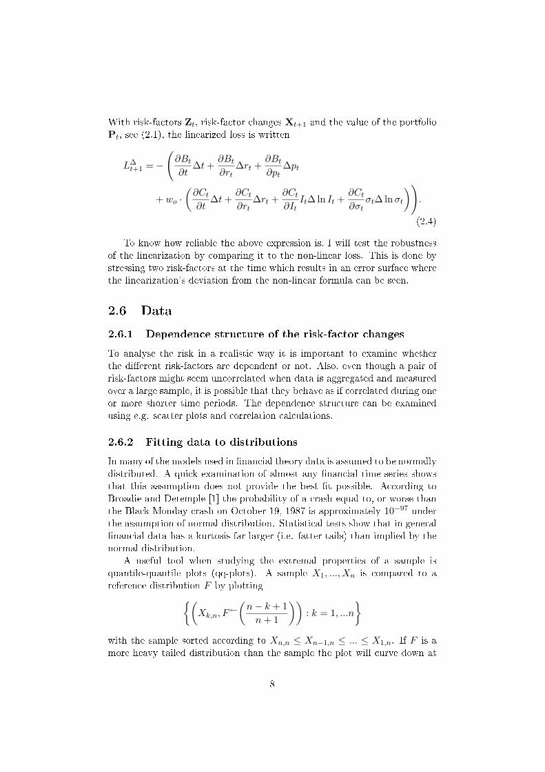
With risk-factors Zt, risk-factor changes Xt+1 and the value of the portfolioPt, see (2.1), the linearized loss is written

L∆t+1 =−

(∂Bt∂t

∆t+∂Bt∂rt

∆rt +∂Bt∂pt

∆pt

+ wo ·(∂Ct∂t

∆t+∂Ct∂rt

∆rt +∂Ct∂It

It∆ ln It +∂Ct∂σt

σt∆ lnσt

)).

(2.4)

To know how reliable the above expression is, I will test the robustnessof the linearization by comparing it to the non-linear loss. This is done bystressing two risk-factors at the time which results in an error surface wherethe linearization's deviation from the non-linear formula can be seen.

2.6 Data

2.6.1 Dependence structure of the risk-factor changes

To analyse the risk in a realistic way it is important to examine whetherthe di�erent risk-factors are dependent or not. Also, even though a pair ofrisk-factors might seem uncorrelated when data is aggregated and measuredover a large sample, it is possible that they behave as if correlated during oneor more shorter time periods. The dependence structure can be examinedusing e.g. scatter plots and correlation calculations.

2.6.2 Fitting data to distributions

In many of the models used in �nancial theory data is assumed to be normallydistributed. A quick examination of almost any �nancial time series showsthat this assumption does not provide the best �t possible. According toBroadie and Detemple [1] the probability of a crash equal to, or worse thanthe Black Monday crash on October 19, 1987 is approximately 10−97 underthe assumption of normal distribution. Statistical tests show that in general�nancial data has a kurtosis far larger (i.e. fatter tails) than implied by thenormal distribution.

A useful tool when studying the extremal properties of a sample isquantile-quantile plots (qq-plots). A sample X1, ..., Xn is compared to areference distribution F by plotting{(

Xk,n, F←(n− k + 1n+ 1

)): k = 1, ...n

}with the sample sorted according to Xn,n ≤ Xn−1,n ≤ ... ≤ X1,n. If F is amore heavy tailed distribution than the sample the plot will curve down at

8

the left and/or up at the right, and the other way around if F has lightertails. If the sample comes from the same distribution as F , the plot appearslinear. More info on qq-plots can be found in Hult and Lindskog [7].

2.7 Risk measurement

The two risk measures that will be used in this thesis are Value-at-Risk andExpected Shortfall. They are de�ned as follows:

VaRα(L) = inf{l ∈ R : P (L > l) ≤ 1− α}= inf{l ∈ R : 1− FL(l) ≤ 1− α}= inf{l ∈ R : FL(l) ≥ α}= F−1

L (α).

ESα(L) = E(L|L ≥ VaRα(L))

=E(LI[qα(L),∞)(L))P(L ≥ qα(L))

=1

1− αE(LI[qα(L),∞)(L))

=1

1− α

∫ ∞qα(L)

ldFL(l).

As stated in the introduction, according to FI the risk on an ELN can be"divided into an interest portion and an equity portion. The risk in theequity portion is that this portion can be positive and then later weakenin a stress scenario". What this basically means is that if the underlyingindex has increased drastically, a "crash" in the index will cause a lot moredamage than if it occurs with the index at approximately the same level asat issuance. With the intention to give a comprehensive risk pro�le of theELN, two risk scenarios are presented below.

2.7.1 Risk scenarios

The ELN portfolio has an initial term to maturity of two years. During thisperiod, two risk scenarios will be considered. One will take place one monthafter issuance, the other one year after issuance. The two scenarios are basedon stressing the two risk-factor pairs (rt, pt) and (ln It, lnσt) one at the timewith the other held constant. The reason for the choice of these pairs is thefact that they are the only two found correlated, see section 3.3.2. Note thatthe scenarios are constructed to show how the risks of the portfolio changedue to changes in the risk-factors, i.e. market conditions, during the periodfrom issuance until just before risk measurement.

9

Risks will be measured for 1-day losses and also 20-day losses whereapplicable. The 1-day losses are chosen to give a sense of the magnitude ofthe day-to-day losses, while the 20-day losses are supposed to represent thefrequency at which a typical investor reviews an investment.

2.7.1.1 Scenario 1 - Stressing (rt, pt)

One month after issuance, the probability that the underlying index hasincreased heavily is low. Therefore, I will consider a scenario where the pair(ln It, lnσt) is held constant (i.e. the same as at issuance) while I allow rtand pt to vary. This leads to a risk function that, instead of being one singlenumber, becomes a surface. This risk surface is dependent on how rt and ptmove during the �rst month. An example of a situation that this scenariocovers is if the Swedish central bank, Riksbanken, decides to change the reporate during this �rst month, and how this changes the risk of the ELN.

2.7.1.2 Scenario 2 - Stressing (ln It, lnσt)

After one year, with one year to maturity, the other scenario takes place.Holding the pair (rt, pt) constant, ln It and lnσt are allowed to vary. Thisgives a risk surface dependent on how ln It and lnσt have moved during the�rst year. For instance, this scenario will show whether the risk increases alot after a period of bullish stock market behaviour.

2.7.2 Historical simulation

Calculating the risk measures with historical simulation is a rather straightforward exercise. Historical data of the risk-factor changes has to be col-lected. Then, the data is simply plugged in to (2.2) which gives the empiricalloss distribution Ln. The empirical VaR and ES can be written

VaRα(Ln) = L[n(1−α)]+1,n

ESα(Ln) =∑[n(1−α)]+1

k=1 Lk,n[n(1− α)] + 1

where [x] is the integer part of x, and with the empirical loss distributionordered such that L1,n ≥ ... ≥ Ln,n.

2.7.3 Analytical solution

For the analytical solution the linearized loss in (2.4) can be used. The partialderivatives of Bt are easily calculated using the bond pricing expression in

10

section 2.4.1. For Ct we need the partial derivatives of the Black-Scholesformula who are the well known Greeks,

∂Ct∂t

is called theta∂Ct∂rt

is called rho

∂Ct∂It

is called delta∂Ct∂σt

is called vega.

The partial derivatives become constants used as weights in the equation.To calculate the risk analytically using one of our preferred risk measures weneed to �nd a multidimensional distribution FXt+1 of the risk-factor changes.This can be done with help of qq-plots, described in section 2.6.2. (2.4) cannow be written

L∆t+1 =−

(∂Bt∂t

+ wo∂Ct∂t

)∆t−

(∂Bt∂rt

+ wo∂Ct∂rt

)∆rt

− ∂Bt∂pt

∆pt − wo∂Ct∂It

It∆ ln It − wo∂Ct∂σt

σt∆ lnσt

=−(∂Bt∂t

+ wo∂Ct∂t

)∆t+ wTXt+1.

If FXt+1 is multivariate elliptically distributed with mean vector µ and co-variance matrix Σ, VaR and ES can be written

VaRα(L∆t+1) =−

(∂Bt∂t

+ wo∂Ct∂t

)∆t+ wTµ

+√

wTΣwVaRα(Xt+1)

=−(∂Bt∂t

+ wo∂Ct∂t

)∆t+ wTµ

+√

wTΣwF−1Xt+1

(α)

and

ESα(L∆t+1) =−

(∂Bt∂t

+ wo∂Ct∂t

)∆t+ wTµ

+√

wTΣwESα(Xt+1)

=−(∂Bt∂t

+ wo∂Ct∂t

)∆t+ wTµ

+√

wTΣw1

1− α

∫ ∞F−1Xt+1

(α)xdFXt+1(x)

where FXt+1 is a one-dimensional standardized elliptical distribution of thesame kind as FXt+1 . For instance, if FXt+1 is multivariate normally dis-tributed then FXt+1 is the standard normal distribution.

11

2.7.4 Monte Carlo simulation

In the Monte Carlo simulation, the value change of the ELN is modelledwith the help of a copula, CR. This is done to achieve a certain dependencestructure of the risk-factor changes. Thereafter, using the best �tted dis-tribution for each of the risk-factor changes one can simulate values of therisk-factor changes from the copula and get simulated "historical data". Therisks are then calculated in the same way as in the historical simulation, seesection 2.7.2. A more detailed description of copulas can be found in Hultand Lindskog [7].

12

Chapter 3

Results

3.1 Creating the structured product

The ELN is created as a portfolio Pt of a bond and wo at-the-money calloptions, see section 2.1. The initial value of the portfolio is set to 100 SEK.The risk-factors were chosen as Zt = (rt, pt, ln It, lnσt). rt is representedby Swedish Treasury bills, SSVX, with 12 months maturity. For the creditrisk premium, pt, I use the so called TED-spread as a proxy. The TED-spread is used as a measure of credit quality and is de�ned as the di�erencebetween the interest rate on interbank loans, in the Swedish case STIBOR,and Treasury bills for a given time to maturity. Applied to the Swedishmarket the equation becomes

TED-spread = STIBOR− SSVX.

It is as previously stated the Swedish equity-index OMXS30TM

. The impliedvolatility σt of the index is represented by DVIS, which is an indicator of theexpected market volatility the following 30 calendar days, calculated fromthe price of OMXS30

TM

options.What remains is to set the initial values of the risk-factors in agreement

with the requirements speci�ed in section 2.1.

Risk-factor Initial valuert 4.4 %pt 0.2 %It 100 SEKσt 24 %

rt and pt are set to their market averages during the examined period. It ischosen out of simplicity, and �nally the implied volatility is set to obtain aparticipation rate, wo, of approximately 0.5.

13

3.2 Maximizing expected utility - An example

Assume that, on a market with three assets, an investor has the utilityfunction U(W1) = ln(W1). Recall that W1 = W0(1 + wT r) is the �nalwealth where W0 is the initial wealth, r = (r1, r2, r3) are the returns of theassets and w = (w1, w2, w3) are the portfolio weights. The investor faces thenonlinear equation system

E

[W0(1 + ri)W0(1 + wT r)

]− λ = 0, i = 1, 2, 3 (3.1)

wT1− 1 = 0.

This can be solved using e.g. MATLAB R©and Newtons Method [5]. 20-day returns of the bond, the index and the call option calculated from thehistorical data, see section 3.3.1, are used to compute the expectation valuesof (3.1). Finally, this yields the portfolio

w1 = 1.4 w2 = −2.1 w3 = 1.7.

The interpretation of this portfolio is that the investor with utility functionln(W1) should short sell 2.1 units of the index, buy 1.4 units of the bond andbuy 1.7 units of the call option on the index. Note that in this example it isassumed that the assets all have the same price.

3.3 Data

3.3.1 Data collection

Data has been collected from a 15 year period, January 1, 1994 to De-cember 31, 2008. 616 days has been left out due to missing data, leavinga total of 3152 days of observations to use in the analysis. rt, pt and Itcan all easily be collected in the market from e.g. www.riksbank.se andfinance.yahoo.com. Regarding σt, the implied volatility-indicator DVIS ispublished on a daily basis by www.derivatinfo.com.

3.3.2 Dependence structure of risk-factor changes

I have investigated the dependence structure of the following pairs of dailyrisk-factor changes.

(∆ ln It,∆ lnσt) (∆rt,∆pt) (∆ ln It,∆rt)(∆ ln It,∆pt) (∆ lnσt,∆rt) (∆ lnσt,∆pt)

Scatter plots of all pairs can be found in �gure 3.1, placed in the sameorder as they are listed above. 250 day rolling correlations for the wholedata set of each pair above have been calculated and can be found in the

14

−0.2 0 0.2−0.2

−0.1

0

0.1

0.2

−10 −5 0 5

x 10−3

−0.01

−0.005

0

0.005

0.01

−0.2 0 0.2−10

−5

0

5x 10

−3

−0.2 0 0.2−0.01

−0.005

0

0.005

0.01

−0.02 −0.01 0 0.01−10

−5

0

5x 10

−3

−0.02 −0.01 0 0.01−0.01

−0.005

0

0.005

0.01

Figure 3.1: Scatter plots of all pairs of risk-factor changes.

appendix, section 5.2. The only pairs that are systematically correlated are(∆ ln It,∆ lnσt) and (∆rt,∆pt), these will instead be presented below andexamined more thoroughly.

3.3.2.1 (∆ ln It,∆ lnσt)

Figure 3.2 shows a 250 day rolling correlation between ∆ ln It and ∆ lnσt.The correlation is negative throughout the whole 15 year period, has anaverage of -0.27 and varies over time between [-0.61, 0].

16−Oct−1995 08−Mar−1999 30−May−2002 04−Oct−2005 15−Dec−2008−1

−0.8

−0.6

−0.4

−0.2

0

0.2

0.4

0.6

0.8

1

Figure 3.2: 250 day rolling correlation of (∆ ln It,∆ lnσt).

15

3.3.2.2 (∆rt,∆pt)

The pair (∆rt,∆pt) has a higher correlation with an average of -0.58, varyingbetween [-0.92 -0.22]. The 250 day rolling correlation can be found in �gure3.3.


−0.8

−0.6

−0.4

−0.2

0

0.2

0.4

0.6

0.8

1

Figure 3.3: 250 day rolling correlation of (∆rt,∆pt).

3.3.3 Fitting data to distributions

Histograms of all four risk-factor changes can be found in �gure 3.4. Allhistograms show a signi�cant di�erence from normal distribution in the waythat they have heavier tails. In �gure 3.5 the reader as a reference �ndshistograms from four di�erent tν-distributions.

3.3.3.1 Distribution of ∆ ln It

In �gure 3.6 ∆ ln It is plotted in qq-plots against nine di�erent tν-distributions.The best �t is provided by the t5.0-distribution, found in the middle of �gure3.6.

3.3.3.2 Distribution of ∆ lnσt

∆ lnσt has heavier tails than ∆ ln It, see �gure 3.4. When qq-plotted againstdi�erent tν-distributions in �gure 3.7, the t2.4-distribution is found to be thebest �t.

16

−0.1 −0.05 0 0.05 0.1 0.150

50

100

150

200

250

−1.5 −1 −0.5 0 0.5 10

200

400

600

−1 −0.5 0 0.50

200

400

600

800

−1 −0.5 0 0.5 10

500

1000

1500

Figure 3.4: Histograms of risk-factor changes. From upper left corner: ∆ ln It,∆ lnσt, ∆rt, ∆pt.

−150 −100 −50 0 50 1000

500

1000

1500

2000

−15 −10 −5 0 5 100

50

100

150

200

250

−10 −5 0 5 100

50

100

150

200

−10 −5 0 5 100

50

100

150

200

Figure 3.5: Histograms from four tν-distributions. From upper left corner:t2, t4, t6, t8

17

−0.2 0 0.2−2000

0

2000

−0.2 0 0.2−20

0

20

−0.2 0 0.2−10

0

10

−0.2 0 0.2−10

0

10

−0.2 0 0.2−10

0

10

−0.2 0 0.2−10

0

10

−0.2 0 0.2−10

0

10

−0.2 0 0.2−10

0

10

−0.2 0 0.2−5

0

5

Figure 3.6: QQ-plots of ∆ ln It vs. tν-distributions. From upper left corner:ν = (1, 3.5, 4, 4.5, 5, 5.5, 6, 6.5, 100).

−2 −1 0 1−2000

0

2000

−2 −1 0 1−200

0

200

−2 −1 0 1−100

0

100

−2 −1 0 1−50

0

50

−2 −1 0 1−50

0

50

−2 −1 0 1−20

0

20

−2 −1 0 1−20

0

20

−2 −1 0 1−20

0

20

−2 −1 0 1−5

0

5

Figure 3.7: QQ-plots of ∆ lnσt vs. tν-distributions. From upper left corner:ν = (1, 1.5, 1.8, 2.1, 2.4, 2.7, 3.0, 3.3, 100).

18

3.3.3.3 Distribution of ∆rt

When making a qq-plot with ∆rt one notices that it is hard to determinewhich distribution provides the best �t, see �gure 3.8, due to the most ex-treme points in the lower left of the �gure. However, the t3.5-distribution isfound to be the best �t.

−1 −0.5 0 0.5−2000

0

2000

−1 −0.5 0 0.5−50

0

50

−1 −0.5 0 0.5−50

0

50

−1 −0.5 0 0.5−20

0

20

−1 −0.5 0 0.5−20

0

20

−1 −0.5 0 0.5−10

0

10

−1 −0.5 0 0.5−10

0

10

−1 −0.5 0 0.5−10

0

10

−1 −0.5 0 0.5−5

0

5

Figure 3.8: QQ-plots of ∆rt vs. tν-distributions. From upper left corner: ν =(1, 2, 2.5, 3, 3.5, 4, 4.5, 5, 100).

3.3.3.4 Distribution of ∆pt

In �gure 3.4 we see that ∆pt is the most heavy tailed risk-factor. The qq-plots in �gure 3.9 indicate that the t2.5-distribution provides the best �t.

3.4 Risk measurement - ELN

In this section the results of the di�erent simulations are presented. Through-out the analysis, the con�dence level α = 0.99 will be used.

Recall that the risks will be measured using the two scenarios de�ned insection 2.7.1 where the risk-factor pairs (rt, pt) and (ln It, lnσt) are stressedone at the time.

3.4.1 Historical simulation

A table with the underlying data for the VaR plots of this section can befound in section 5.3 in the appendix.

19

−1 0 1−2000

0

2000

−1 0 1−100

0

100

−1 0 1−50

0

50

−1 0 1−50

0

50

−1 0 1−50

0

50

−1 0 1−20

0

20

−1 0 1−20

0

20

−1 0 1−20

0

20

−1 0 1−5

0

5

Figure 3.9: QQ-plots of ∆pt vs. tν-distributions. From upper left corner: ν =(1, 1.6, 1.9.2.2, 2.5, 2.8, 3.1, 3.4, 100).


The results can be found in �gures 3.10 and 3.11.

00.1

0.20.3

0.4

33.5

44.5

55.5

1.6

1.7

1.8

1.9

2

TED [%]Rate [%]

1D V

aR &

ES

[SE

K]

Figure 3.10: Scenario 1 with historical simulation, 1-day VaR and ES. The risklevels are fairly constant throughout the whole surfaces.


The results are found in �gures 3.12 and 3.13.

20

00.1

0.20.3

0.4

33.5

44.5

55.5

3.1

3.2

3.3

3.4

3.5

3.6

TED [%]Rate [%]

20D

VaR

& E

S [S

EK

]

Figure 3.11: Scenario 1 with historical simulation, 20-day VaR and ES. As in thecase for the 1-day risks, the changes in the risks over the surfaces are small.

6080

100120

140160

180200

10

20

30

40

1

2

3

4

5

Index [SEK]Volatility [%]

1D V

aR &

ES

[SE

K]

Figure 3.12: Scenario 2 with historical simulation, 1-day VaR and ES. Note thatthe changes in the index have a large e�ect on the risk level. The level of the impliedvolatility has di�erent e�ects on the risk depending on the index level.

21

6080

100120

140160

180200

10

20

30

40

5

10

15


20D

VaR

& E

S [S

EK

]

Figure 3.13: Scenario 2 with historical simulation, 20-day VaR and ES. As in thecase of the 1-day risks, the index has a huge impact on the risk level. Note thatthe risks dependence on the implied volatility is weaker than in the 1-day case.

22

3.4.2 Robustness of the linearization

The error of the linearization is calculated as the relative di�erence betweenthe linearized loss (2.3) and the non-linear loss (2.2), (L∆

t+1 − Lt+1)/(Lt+1).Hence, the error is a function of the risk-factors. The linearization is testedby stressing the risk-factor pairs (rt, pt) and (ln It, lnσt) one at the time. Theresults can be found in �gures 3.14 and 3.15. Note that the centre points ofthe x-axis and y-axis corresponds to a zero loss where naturally the error iszero. Due to the characteristics of these �gures the 20-day risks calculatedwith the linearized analytical solution will not be used.

−0.20

0.20.4

0.6

3.54

4.55

5.50

0.5

1

1.5

2

TED [%]Rate [%]

Rel

ativ

e er

ror

[%]

Figure 3.14: Robustness of the linearization. The relative error caused by stress-ing the risk-factor pair (rt, pt).

3.4.3 Analytical solution

Using the distributions found in section 3.3.3 one can conclude that the mul-tivariate elliptical distribution FXt+1 , and hence the marginal distributionFX1 , can be approximated by a t3 distribution. The analytical VaR and ESis then written

VaR0.99(L∆t+1) =−

(∂Bt∂t

+ wo∂Ct∂t

)∆t+ wTµ

+√

wTΣwVaR0.99(Xt+1)

=−(∂Bt∂t

+ wo∂Ct∂t

)∆t+ wTµ

+√

wTΣwF−1t3

(0.99)

23

94 96 98 100 102 104 106

2025

3035

−16

−14

−12

−10

−8

−6

−4

−2

0


Rel

ativ

e er

ror

[%]

Figure 3.15: Robustness of the linearization. The relative error caused by stress-ing the risk-factor pair (ln It, lnσt).

and

ES0.99(L∆t+1) =−

(∂Bt∂t

+ wo∂Ct∂t

)∆t+ wTµ

+√

wTΣwES0.99(Xt+1)

=−(∂Bt∂t

+ wo∂Ct∂t

)∆t+ wTµ

+√

wTΣw1

1− 0.99

∫ ∞F−1t3

(0.99)xdFt3(x).


The result is found in �gure 3.16.


The result is found in �gure 3.17.

24

00.1

0.20.3

0.4

33.5

44.5

55.5

1.6

1.8

2

2.2

2.4

TED [%]Rate [%]

1D V

aR &

ES

[SE

K]

Figure 3.16: Scenario 1 with analytical solution, 1-day VaR and ES. As in thehistorical simulation, the risk surfaces are quite �at.

6080

100120

140160

180200

10

20

30

40

1

2

3

4

5

6


1D V

aR &

ES

[SE

K]

Figure 3.17: Scenario 2 with analytical solution, 1-day VaR and ES. The be-haviour is quite similar to the historical simulation, although the surfaces aresmoother.

25

3.4.4 Monte Carlo simulation

As in section 3.4.3 we approximate the multivariate distribution as t3. Thegeneration of the 4-dimensional t-copula Ct3,R can be summarized in thefollowing eight steps:

1. Measure pairwise dependence between risk-factor changes.

2. Collect in a 4-by-4 dependence matrix R.

3. Find the Cholesky decomposition A of R where R = AAT.

4. Simulate 4 independent random variates Z1,...,Z4 from N(0,1).

5. Simulate a random variate S from χ23.

6. Set Y = AZ and X =√

3√SY.

7. Set Uk = t3(Xk) for k = 1, ..., 4.

8. Start over from 4.

This is iterated a desirable number of times to yield a sample from thecopula Ct3,R. In �gure 3.18 pairwise scatter plots of the risk-factor changessimulated from the copula can be found. If these are compared with thepairwise scatter plots of the original data in �gure 3.1 one can see that theyare quite similar.

−0.1 0 0.1−5

0

5

10x 10

−3

−5 0 5

x 10−3

−4

−2

0

2

4x 10

−3

−0.1 0 0.1−6

−4

−2

0

2

4x 10

−3

−0.1 0 0.1−4

−2

0

2

4x 10

−3

−5 0 5 10

x 10−3

−6

−4

−2

0

2

4x 10

−3

−4 −2 0 2 4 6 8 10

x 10−3

−4

−3

−2

−1

0

1

2

3

4x 10

−3

Figure 3.18: Pairwise scatter plots of copula parameters, ordered in the same wayas originally listed in page 14.

26


Value-at-Risk and Expected Shortfall calculated with a Monte Carlo simu-lation can be found in �gures 3.19 and 3.20.

00.1

0.20.3

0.4

33.5

44.5

55.5

0.95

1

1.05

1.1

1.15

1.2

1.25

1.3

TED [%]Rate [%]

1D V

aR &

ES

[SE

K]

Figure 3.19: Scenario 1 with Monte Carlo simulation, 1-day VaR and ES. TheMonte Carlo analysis con�rms the results provided by the previous methods.

00.1

0.20.3

0.4

33.5

44.5

55.5

3.2

3.4

3.6

3.8

4

TED [%]Rate [%]

20D

VaR

& E

S [S

EK

]

Figure 3.20: Scenario 1 with Monte Carlo simulation, 20-day VaR and ES.


Value-at-Risk and Expected Shortfall calculated with a Monte Carlo simu-lation can be found in �gures 3.21 and 3.22.

27

6080

100120

140160

180200

10

20

30

40

0.5

1

1.5

2

2.5

3

3.5


1D V

aR &

ES

[SE

K]

Figure 3.21: Scenario 2 with Monte Carlo simulation, 1-day VaR and ES. Alsoin this second scenario, the results of the previous sections are con�rmed. The risksurfaces are a�ected drastically by changes in the index.

6080

100120

140160

180200

10

20

30

40

0

2

4

6

8

10

12


20D

VaR

& E

S [S

EK

]

Figure 3.22: Scenario 2 with Monte Carlo simulation, 20-day VaR and ES.

28

3.4.5 A recapitulation of the ELN results

The stress tests are divided into two di�erent scenarios where the risk-factorpairs (∆rt,∆pt) and (∆ ln It,∆ lnσt) are stressed one at the time. Thestress tests are performed with historical simulation, computed analyticallyand with a Monte Carlo simulation. All three methods give approximatelythe same results throughout the analysis for both VaR and ES. Therefore,only the 1-day VaR from the historical simulation will be referred to below.

3.4.5.1 Analysis of Scenario 1 - Stressing (∆rt,∆pt)

Figure 3.10 shows that the risks are fairly constant over the whole surface,which is almost a plane. The lowest risk on the surface is in the cornerwith high interest rate rt and high credit risk premium pt. The maximumdi�erence over the whole VaR surface is 2.5 percent and hence, the changesin the risks are very much controllable.

3.4.5.2 Analysis of Scenario 2 - Stressing (∆ ln It,∆ lnσt)

Changes in the index It has large implications to the risk level. The 1-dayrisk surface, see �gure 3.12, shows that from the starting point at It = 100,the risk increases with 219 percent when It is doubled to 200. And if It ishalved to 50, the risk decreases with 93 percent. The implied volatility σtdoes also have an e�ect on the risk, but it varies with It. With index between50 and 100, a high implied volatility causes higher risk. Then with indexbetween 120 and 150, the exact opposite occurs. Hence, this scenario causesmajor changes to the risk level of the ELN.

3.5 Risk measurement - Bond-Stock portfolios

Risks are, as in the case with the ELN, measured using the two scenar-ios de�ned in section 2.7.1. Since the results of the ELN were consistentthroughout the analysis above, the risks of the Bond-Stock portfolios willonly be measured with historical simulation.

As for the ELN, a table with the underlying data for the 1-day VaR plotsof this section can be found in section 5.3 in the appendix.



The results of the scenario 1 simulations of Bond-Stock portfolio 1 can befound in �gures 3.23 and 3.24.

29

00.1

0.20.3

0.4

33.5

44.5

55.5

2.1

2.2

2.3

2.4

2.5

TED [%]Rate [%]

1D V

aR &

ES

[SE

K]

Figure 3.23: Scenario 1 with Bond-Stock portfolio 1, 1-day VaR and ES. The risksurfaces look similar to the ones of the ELN.

00.1

0.20.3

0.4

33.5

44.5

55.5

7

7.5

8

8.5

9

TED [%]Rate [%]

20D

VaR

& E

S [S

EK

]

Figure 3.24: Scenario 1 with Bond-Stock portfolio 1, 20-day VaR and ES.

30


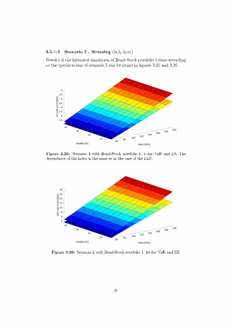
Results of the historical simulation of Bond-Stock portfolio 1 done accordingto the speci�cations of scenario 2 can be found in �gures 3.25 and 3.26.

6080

100120

140160

180200

10

20

30

40

1.5

2

2.5

3

3.5

4

4.5

5


1D V

aR &

ES

[SE

K]

Figure 3.25: Scenario 2 with Bond-Stock portfolio 1, 1-day VaR and ES. Thedependence of the index is the same as in the case of the ELN.

6080

100120

140160

180200

10

20

30

40

4

6

8

10

12

14

16

18


20D

VaR

& E

S [S

EK

]


31



Scenario 1 results of the historical simulation of Bond-Stock portfolio 2 canbe found in �gures 3.27 and 3.28.

00.1

0.20.3

0.4

33.5

44.5

55.5

0.36

0.38

0.4

0.42

0.44

0.46

TED [%]Rate [%]

1D V

aR &

ES

[SE

K]


00.1

0.20.3

0.4

33.5

44.5

55.5

1.1

1.2

1.3

1.4

1.5

TED [%]Rate [%]

20D

VaR

& E

S [S

EK

]


32


Results of scenario 2 simulations of Bond-Stock portfolio 2 can be found in�gures 3.29 and 3.30.

6080

100120

140160

180200

10

20

30

40

0.2

0.3

0.4

0.5

0.6

0.7

0.8


1D V

aR &

ES

[SE

K]

Figure 3.29: Scenario 2 with Bond-Stock portfolio 2, 1-day VaR and ES. The risksurfaces shows the same behaviour as Bond-Stock portfolio 1.

6080

100120

140160

180200

10

20

30

40

1

1.5

2

2.5

3


20D

VaR

& E

S [S

EK

]


3.5.3 A recapitulation of the B-S portfolio results

The risk pro�les of the two Bond-Stock portfolios, below called B-S 1 andB-S 2, are examined in the same way as the ELN. Recall that B-S 1 has the

33

same participation rate as the ELN, and that B-S 2 has the same guaranteedpayout as the ELN. In this recapitulation only 1-day VaR from the historicalsimulation is considered.

3.5.3.1 Analysis of Scenario 1 - Stressing (∆rt,∆pt)

Just like in the case of the ELN, the risk surfaces on both B-S 1 and B-S2 are very close to being planes. The maximum di�erence between any twopoints on the two portfolios' risk surfaces are 0.4 percent for B-S 1 and 4.7percent for B-S 2. As in the case for the ELN, the lowest risk on the surfacesis found at high interest rate rt and high credit risk premium pt. Hence, thisscenario only causes small changes in the risk level.

3.5.3.2 Analysis of Scenario 2 - Stressing (∆ ln It,∆ lnσt)

In contrary to the ELN, the implied volatility does not have an e�ect on therisk surfaces. Changes in the index has a big impact on both portfolios. B-S1 shows an increase of risk with 106 percent when the index is doubled, anda decrease of 45 percent when the index is halved. B-S 2 shows the samepattern but the numbers are a 112 percent increase and a 44 percent decreaserespectively. This scenario causes signi�cant changes in the risk level of theportfolios, but not to the extent of the ELN case.

3.6 Comparing the ELN to the B-S portfolios

3.6.1 The risk surfaces

The most extreme changes in the risks, both for the ELN as well as theBond-Stock portfolios has occurred when stressing according to Scenario 2.Therefore, a graphical comparison of the 1-day VaR of the ELN and eachof the Bond-Stock portfolios can be found in �gures 3.31 and 3.32. Thecomparisons are presented as di�erences between the ELN and each of theBond-Stock portfolios and calculated as VaRELN −VaRB-S i, where i = 1, 2.

3.6.2 The portfolios' values

To put the risk measurement of all three portfolios, ELN, B-S 1 and B-S 2,into a bigger picture it is valuable to have an idea about how the values ofthe portfolios change with the index. This is done both with one year tomaturity as well as at maturity and can be found in �gures 3.33 and 3.34.

No transaction fees has been taken into account for the two Bond-Stockportfolios, but for the ELN a 2 percent upfront fee has been applied to re�ectthe di�erence in brokerage fees between the ELN and the B-S portfolios. To�nd a reasonable number to use, this has been discussed with a previousemployee at one of the larger issuers of ELNs in Sweden.

34

6080

100120

140160

180200

10

20

30

40

−1.5

−1

−0.5

0


Δ 1D

VaR

[SE

K]

Figure 3.31: Comparing the risk surfaces of the ELN and B-S 1. This illuminatesthe di�erence in how the two portfolios depend on the implied volatility. The riskof the ELN is lower at almost the whole surface, although at low volatility and highindex levels the di�erence is approximately zero.

6080

100120

140160

180200

10

20

30

40

0

0.5

1

1.5

2

2.5

3


Δ 1D

VaR

[SE

K]

Figure 3.32: Comparing the risk surfaces of the ELN and B-S 2. Note that therisk of the ELN is higher at almost the whole surface, but at low volatility and lowindex levels the di�erence is approximately zero.

35

40 60 80 100 120 140 160 180 200 22070

80

90

100

110

120

130

140

150

160

Index [SEK]

Val

ue [S

EK

]

ELNB−S 1B−S 2

Figure 3.33: Comparing the values of the portfolios as the underlying index changewith one year to maturity. Note that the ELN never has the highest value, andthat between the index values of 89 SEK and 118 SEK it actually has the lowestvalue. The dashed line is the ELN without the upfront fee.

40 60 80 100 120 140 160 180 200 22070

80

90

100

110

120

130

140

150

160

Index [SEK]

Val

ue [S

EK

]

ELNB−S 1B−S 2

Figure 3.34: Comparing the values of the portfolios as the underlying index changeat maturity. Note that the ELN never has the highest value, and that between theindex values of 86 SEK and 127 SEK it actually has the lowest value. The dashedline is the ELN without the upfront fee.

36

Chapter 4

Conclusions and Discussion

4.1 ELN versus Bond-Stock portfolios

First of all, the goals with this thesis are to give a comprehensive risk pro�leof the ELN and to compare the ELN to alternative investments. To a largeextent the risk pro�les of the ELN as well as the two Bond-Stock portfoliosare presented in the results chapter in terms of �gures and the two recapitu-lations. Therefore, this section will most of all be focused on comparing theELN to the Bond-Stock portfolios. This can be done using table 4.1 whichprovides a summary of the two recapitulations of the results chapter. Fromthe results of the analysis it can be seen that the risk-factor with the largestin�uence on the risks of both the ELN and the Bond-Stock portfolios is theindex. As we see in table 4.1 the risk of the ELN can change signi�cantly

Portfolio Scenario 1 Scenario 2 Scenario 2Max ∆ It: 100 → 200 It: 100 → 50

ELN 2.5% 219% -93%B-S 1 0.4% 106% -45%B-S 2 4.7% 112% -44%

Table 4.1: The table provides a summary of the two recapitulations in the pre-vious chapter. Max ∆ denotes the maximum di�erence in risk over a Scenario1 risk surface. It: 100 → 200 and It: 100 → 50 shows how much the risk in-creases(decreases) when the index is doubled(halved) in Scenario 2.

with changing market conditions. When it is stressed according to scenario2 and the index is doubled, the risk level increases by 219 percent. When theindex is halved, the risk level decreases to 7 percent of the initial value. Thesame behaviour occurs for both of the Bond-Stock portfolios, although notto the same extent. As seen in section 3.6.1, at high index levels the ELNhas a risk level approximately equal to B-S 1, and at low index levels therisk level is similar to B-S 2. This behavior is repeated if we look at �gure

37

3.33 showing the values as functions of the index of the three portfolios. Thecharacteristics of this �gure shows that at low index levels the value func-tions of the ELN and B-S 2 are approximately parallel and at high indexlevels the value functions of the ELN and B-S 1 are parallel.

The ELN can be thought of as an "insurance" that gives the behaviorof a B-S 1 portfolio in a bull market, and the behavior of a B-S 2 portfolioin a bear market. For this insurance the investor has to pay a premium. In�gure 3.34 the ELN never has the highest value of the three portfolios, andbetween the index levels of 86 SEK and 127 SEK it has the lowest value.An analysis of the 15 years of OMXS30

TM

data used in this thesis shows thatwith a probability of 67 percent the index, starting at 100, gives a two yearreturn within the interval [86 127], the interval in which the ELN gives thelowest return.

I believe that an ELN would be considered a safe investment by mostinvestors, since with a two year time horizon the worst thing that can happenis that the investor gets the initial capital back. Two major setbacks of theELN seem to be the risk of losing the interest rate normally paid by a bondand the high upfront fee charged.

4.2 Final re�ections

Some investors might be looking for "The opportunity to a good return withthe safety of the bond", meaning they will refrain the interest rate normallypaid by a bond to instead bet on an eventual market increase. Other investorswill set a risk level according to their �nancial goals, and others again willspecify their utility function and optimize their portfolio accordingly.

For the second category of investors, an ELN will cause some problems.To keep the risk at a nearly constant level, the opportunity to easily rebal-ance the portfolio is important. The same problem occurs for the investorwho has optimized a portfolio given a utility function. Once the values ofthe portfolio components starts to move, a rebalancing is needed. Easy re-balancing includes both low transaction costs as well as a liquid market forthe assets, of which neither are typical features of the ELN.

Finally, for a very passive investor, i.e. one that wants to buy a portfolioand forget about it for two years, the risk of losing the interest rate andgetting charged the upfront fee are premiums worth paying, but for investors'who keeps fairly good track of their portfolios it appears more rational toinvest in a portfolio consisting of a combination of the bond and the index.

38

Chapter 5

Appendix

5.1 Plots of the Risk-factors

25−Oct−1994 19−Mar−1998 05−Dec−2001 15−Jul−2005 30−Dec−20080

200

400

600

800

1000

1200

1400

1600

[SE

K]

Figure 5.1: Daily quotes of It between January 1 1994 to December 31 2008 withbad data removed.

39


10

20

30

40

50

60

70

80

[%]

Figure 5.2: Daily quotes of σt between January 1 1994 to December 31 2008 withbad data removed.


2

4

6

8

10

[%]

Figure 5.3: Daily quotes of rt between January 1 1994 to December 31 2008 withbad data removed.

40


0

0.5

1

1.5

2

2.5

[%]

Figure 5.4: Daily quotes of pt between January 1 1994 to December 31 2008 withbad data removed.

41

5.2 Additional rolling correlations


−0.8

−0.6

−0.4

−0.2

0

0.2

0.4

0.6

0.8

1

Figure 5.5: 250 day rolling correlation of (∆ ln It, rt).


−0.8

−0.6

−0.4

−0.2

0

0.2

0.4

0.6

0.8

1

Figure 5.6: 250 day rolling correlation of (∆ ln It, pt).

42


−0.8

−0.6

−0.4

−0.2

0

0.2

0.4

0.6

0.8

1

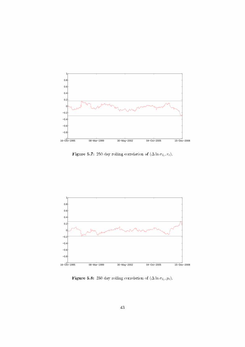
Figure 5.7: 250 day rolling correlation of (∆ lnσIt, rt).


−0.8

−0.6

−0.4

−0.2

0

0.2

0.4

0.6

0.8

1

Figure 5.8: 250 day rolling correlation of (∆ lnσIt, pt).

43

5.3 Risk measurement - Data from �gures

In this section, underlying data of the VaR from the �gures in the historicalsimulation section in the Results chapter are presented.

5.3.1 ELN - Scenario 1

pt -0.05 0 0.05 0.10 0.15 0.20 0.25 0.30 0.35 0.40 0.45rt2.90 1.54 1.54 1.54 1.54 1.54 1.54 1.54 1.54 1.54 1.54 1.543.20 1.54 1.54 1.54 1.54 1.54 1.54 1.54 1.54 1.54 1.54 1.543.50 1.53 1.53 1.53 1.53 1.53 1.53 1.53 1.53 1.53 1.53 1.533.80 1.53 1.53 1.53 1.53 1.53 1.53 1.53 1.53 1.53 1.53 1.534.10 1.55 1.55 1.55 1.55 1.55 1.54 1.54 1.54 1.54 1.54 1.544.40 1.55 1.55 1.55 1.55 1.55 1.55 1.55 1.55 1.55 1.55 1.554.70 1.54 1.54 1.54 1.54 1.54 1.54 1.54 1.54 1.54 1.54 1.545.00 1.53 1.53 1.53 1.53 1.53 1.53 1.53 1.53 1.53 1.53 1.535.30 1.53 1.53 1.53 1.53 1.53 1.52 1.52 1.52 1.52 1.52 1.525.60 1.52 1.52 1.52 1.52 1.52 1.52 1.52 1.52 1.52 1.52 1.525.90 1.51 1.51 1.51 1.51 1.51 1.51 1.51 1.51 1.51 1.51 1.51

Table 5.1: Underlying data from Scenario 1, �gure 3.10 showing 1-day losses fromthe historical simulation.

pt -0.05 0 0.05 0.10 0.15 0.20 0.25 0.30 0.35 0.40 0.45rt2.90 3.07 3.07 3.07 3.06 3.06 3.06 3.06 3.05 3.05 3.05 3.053.20 3.10 3.10 3.09 3.09 3.09 3.09 3.09 3.08 3.08 3.08 3.083.50 3.13 3.13 3.13 3.12 3.12 3.12 3.12 3.11 3.11 3.11 3.113.80 3.15 3.15 3.15 3.15 3.14 3.14 3.14 3.14 3.13 3.13 3.134.10 3.19 3.19 3.18 3.18 3.18 3.18 3.18 3.17 3.17 3.17 3.174.40 3.22 3.22 3.21 3.21 3.21 3.21 3.21 3.20 3.20 3.20 3.204.70 3.23 3.23 3.23 3.22 3.22 3.22 3.21 3.21 3.21 3.20 3.205.00 3.25 3.24 3.24 3.24 3.24 3.24 3.24 3.24 3.23 3.23 3.235.30 3.28 3.28 3.28 3.28 3.27 3.27 3.27 3.27 3.26 3.26 3.265.60 3.30 3.30 3.29 3.29 3.29 3.29 3.29 3.29 3.28 3.28 3.285.90 3.32 3.32 3.32 3.32 3.32 3.32 3.31 3.31 3.31 3.31 3.31

Table 5.2: Underlying data from Scenario 1, �gure 3.11 showing 20-day lossesfrom the historical simulation.

44

5.3.2 ELN - Scenario 2

It 55 70 85 100 115 130 145 160 175 190 205σt4 0.09 0.09 0.09 1.40 2.36 2.66 2.96 3.27 3.57 3.88 4.188 0.09 0.09 0.12 1.15 2.27 2.66 2.96 3.27 3.57 3.88 4.1812 0.09 0.09 0.27 1.11 2.02 2.63 2.95 3.27 3.57 3.88 4.1816 0.09 0.10 0.45 1.10 1.84 2.46 2.94 3.26 3.57 3.88 4.1820 0.09 0.15 0.61 1.18 1.71 2.29 2.81 3.24 3.57 3.88 4.1824 0.10 0.28 0.78 1.31 1.64 2.15 2.63 3.12 3.53 3.88 4.1828 0.11 0.42 0.95 1.38 1.63 2.07 2.53 2.95 3.41 3.81 4.1832 0.15 0.57 1.10 1.49 1.70 1.99 2.44 2.85 3.25 3.69 4.0636 0.24 0.73 1.24 1.55 1.88 2.00 2.32 2.75 3.14 3.53 3.9640 0.34 0.88 1.38 1.66 1.90 1.99 2.30 2.68 3.06 3.42 3.8044 0.46 1.04 1.49 1.81 2.05 2.11 2.31 2.61 2.98 3.35 3.69

Table 5.3: Underlying data from Scenario 2, �gure 3.12 showing 1-day losses fromthe historical simulation.

It 55 70 85 100 115 130 145 160 175 190 205σt4 0.15 0.15 0.11 2.11 7.50 9.03 10.08 11.13 12.18 13.22 14.278 0.15 0.15 0.15 2.36 6.65 8.83 10.04 11.13 12.18 13.22 14.2712 0.15 0.13 0.37 2.54 5.85 8.42 9.89 11.08 12.15 13.22 14.2716 0.15 0.12 0.65 2.66 5.44 7.71 9.58 10.90 12.12 13.18 14.2320 0.13 0.17 0.94 2.74 5.03 7.15 9.02 10.62 11.87 13.07 14.2224 0.12 0.30 1.22 2.78 4.84 6.81 8.54 10.11 11.62 12.81 14.0628 0.12 0.46 1.47 2.92 4.62 6.38 8.09 9.73 11.13 12.60 13.7232 0.17 0.65 1.70 2.99 4.52 6.16 7.75 9.18 10.78 12.11 13.4336 0.25 0.88 1.91 3.08 4.41 6.04 7.34 8.96 10.18 11.79 13.0840 0.36 1.12 2.12 3.19 4.42 5.84 7.21 8.62 9.99 11.14 12.7644 0.50 1.35 2.31 3.28 4.42 5.68 7.11 8.33 9.65 10.97 12.07

Table 5.4: Underlying data from Scenario 2, �gure 3.13 showing 20-day lossesfrom the historical simulation.

45

5.3.3 Bond-Stock portfolios - Scenario 1

pt -0.05 0 0.05 0.10 0.15 0.20 0.25 0.30 0.35 0.40 0.45rt2.90 2.05 2.05 2.04 2.04 2.04 2.04 2.04 2.04 2.04 2.04 2.043.20 2.04 2.04 2.04 2.04 2.04 2.04 2.04 2.04 2.04 2.04 2.043.50 2.04 2.04 2.04 2.04 2.04 2.04 2.04 2.04 2.04 2.04 2.043.80 2.04 2.04 2.04 2.04 2.04 2.04 2.04 2.04 2.04 2.04 2.044.10 2.04 2.04 2.04 2.04 2.04 2.04 2.04 2.04 2.04 2.04 2.044.40 2.04 2.04 2.04 2.04 2.04 2.04 2.04 2.04 2.04 2.04 2.044.70 2.04 2.04 2.04 2.04 2.04 2.04 2.04 2.04 2.04 2.04 2.045.00 2.04 2.04 2.04 2.04 2.04 2.04 2.04 2.04 2.04 2.04 2.045.30 2.04 2.04 2.04 2.04 2.04 2.04 2.04 2.04 2.04 2.04 2.045.60 2.04 2.04 2.04 2.04 2.04 2.04 2.04 2.04 2.04 2.04 2.045.90 2.04 2.04 2.04 2.04 2.04 2.04 2.04 2.04 2.04 2.04 2.04

Table 5.5: Underlying data from Scenario 1, �gure 3.23 showing 1-day losses fromthe B-S 1 portfolio.

pt -0.05 0 0.05 0.10 0.15 0.20 0.25 0.30 0.35 0.40 0.45rt2.90 0.37 0.37 0.37 0.37 0.37 0.37 0.37 0.36 0.36 0.36 0.363.20 0.37 0.36 0.36 0.36 0.36 0.36 0.36 0.36 0.36 0.36 0.363.50 0.36 0.36 0.36 0.36 0.36 0.36 0.36 0.36 0.36 0.36 0.363.80 0.36 0.36 0.36 0.36 0.36 0.36 0.36 0.36 0.36 0.36 0.364.10 0.36 0.36 0.36 0.36 0.36 0.36 0.36 0.36 0.36 0.36 0.364.40 0.36 0.36 0.36 0.36 0.36 0.36 0.36 0.36 0.36 0.36 0.364.70 0.36 0.36 0.36 0.36 0.36 0.36 0.36 0.36 0.35 0.35 0.355.00 0.36 0.36 0.35 0.35 0.35 0.35 0.35 0.35 0.35 0.35 0.355.30 0.35 0.35 0.35 0.35 0.35 0.35 0.35 0.35 0.35 0.35 0.355.60 0.35 0.35 0.35 0.35 0.35 0.35 0.35 0.35 0.35 0.35 0.355.90 0.35 0.35 0.35 0.35 0.35 0.35 0.35 0.35 0.35 0.35 0.35


46

5.3.4 Bond-Stock portfolios - Scenario 2

It 55 70 85 100 115 130 145 160 175 190 205σt4 1.12 1.42 1.73 2.03 2.34 2.65 2.95 3.26 3.57 3.87 4.188 1.12 1.42 1.73 2.03 2.34 2.65 2.95 3.26 3.57 3.87 4.1812 1.12 1.42 1.73 2.03 2.34 2.65 2.95 3.26 3.57 3.87 4.1816 1.12 1.42 1.73 2.03 2.34 2.65 2.95 3.26 3.57 3.87 4.1820 1.12 1.42 1.73 2.03 2.34 2.65 2.95 3.26 3.57 3.87 4.1824 1.12 1.42 1.73 2.03 2.34 2.65 2.95 3.26 3.57 3.87 4.1828 1.12 1.42 1.73 2.03 2.34 2.65 2.95 3.26 3.57 3.87 4.1832 1.12 1.42 1.73 2.03 2.34 2.65 2.95 3.26 3.57 3.87 4.1836 1.12 1.42 1.73 2.03 2.34 2.65 2.95 3.26 3.57 3.87 4.1840 1.12 1.42 1.73 2.03 2.34 2.65 2.95 3.26 3.57 3.87 4.1844 1.12 1.42 1.73 2.03 2.34 2.65 2.95 3.26 3.57 3.87 4.18


It 55 70 85 100 115 130 145 160 175 190 205σt4 0.19 0.24 0.29 0.34 0.39 0.44 0.50 0.55 0.60 0.66 0.718 0.19 0.24 0.29 0.34 0.39 0.44 0.50 0.55 0.60 0.66 0.7112 0.19 0.24 0.29 0.34 0.39 0.44 0.50 0.55 0.60 0.66 0.7116 0.19 0.24 0.29 0.34 0.39 0.44 0.50 0.55 0.60 0.66 0.7120 0.19 0.24 0.29 0.34 0.39 0.44 0.50 0.55 0.60 0.66 0.7124 0.19 0.24 0.29 0.34 0.39 0.44 0.50 0.55 0.60 0.66 0.7128 0.19 0.24 0.29 0.34 0.39 0.44 0.50 0.55 0.60 0.66 0.7132 0.19 0.24 0.29 0.34 0.39 0.44 0.50 0.55 0.60 0.66 0.7136 0.19 0.24 0.29 0.34 0.39 0.44 0.50 0.55 0.60 0.66 0.7140 0.19 0.24 0.29 0.34 0.39 0.44 0.50 0.55 0.60 0.66 0.7144 0.19 0.24 0.29 0.34 0.39 0.44 0.50 0.55 0.60 0.66 0.71


47

Bibliography

[1] Broadie, M., Detemple, J.B. (2004) Option Pricing: Valuation Models

and Applications. Management Science Vol. 50, No. 9.

[2] Euroclear Sweden. (2009) Total volume of index-linked notes.www.ncsd.eu.

[3] Euroclear Sweden. (2009) Report of issued volumes of ELNs in 2008,

denominated in SEK. www.ncsd.eu.

[4] Grundberg, Sven. (2008) Allt mer pengar investeras i aktieindexobliga-

tioner. www.e24.se.

[5] Heath, Michael .T. (2002) Scienti�c Computing - An Introductory Sur-

vey. McGraw Hill.

[6] Hull, J.C. (2006) Options, Futures and Other Derivatives, Sixth Edition.Prentice-Hall.

[7] Hult, H., Lindskog, F. (2007) Mathematical Modeling and Statistical

Methods for Risk Management - Lecture Notes. Lecture Notes fromcourse Risk Management at Royal Institute of Technology.

[8] Luenberger, David G. (1998) Investment Science. Oxford UniversityPress.

[9] SEB. (2009) Sales material published on SEB's website 2009-03-11.http://www.seb.se/pow/kampanjer/kapitalskydd/pdf/broschyr.pdf.

[10] Swedish Financial Supervisory Authority. (2006) Equity-linked bonds -

an evaluation of the new prospectus rules. www.�.se.

[11] Öhrn, Linda. (2008) Stabilitetsplan dödsstöt för aktieindexobligationer.www.di.se.

48

risk analysis of structured products - kth

Documents