risk and exposure by apte

8/4/2019 Risk and Exposure by Apte

http://slidepdf.com/reader/full/risk-and-exposure-by-apte 1/22

InvestmentsLecture 4: Hedging Interest Rate Risk Exposure

Traditional Methods

Philip H. DybvigWashington University in Saint Louis

• Matching maturities

• Duration

• Effective duration

•Multiple duration measures

Copyright c Philip H. Dybvig 2000



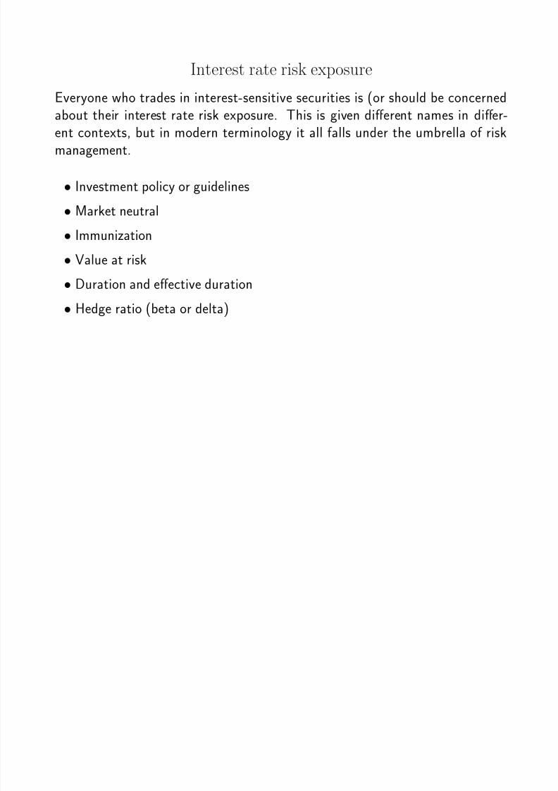
Interest rate risk exposure

Everyone who trades in interest-sensitive securities is (or should be concernedabout their interest rate risk exposure. This is given different names in differ-ent contexts, but in modern terminology it all falls under the umbrella of riskmanagement.

• Investment policy or guidelines

• Market neutral

• Immunization

• Value at risk

•Duration and effective duration

• Hedge ratio (beta or delta)



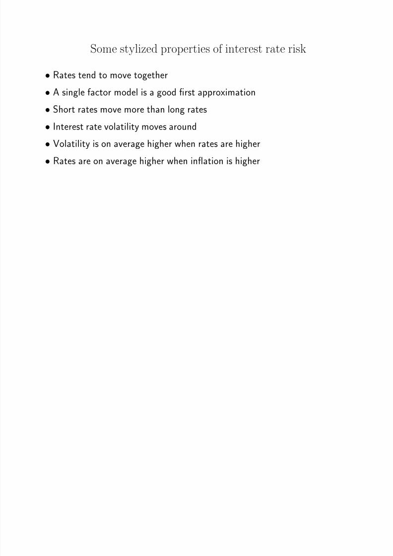
Some stylized properties of interest rate risk

• Rates tend to move together

• A single factor model is a good first approximation

• Short rates move more than long rates

• Interest rate volatility moves around

• Volatility is on average higher when rates are higher

• Rates are on average higher when inflation is higher



Matching cash flows

Advantages:

• Simple

• Reliable

Disadvantages:

• Cannot hedge complex bonds or derivatives

• No obvious corresponding risk measure

• May over-hedge and incur high costs



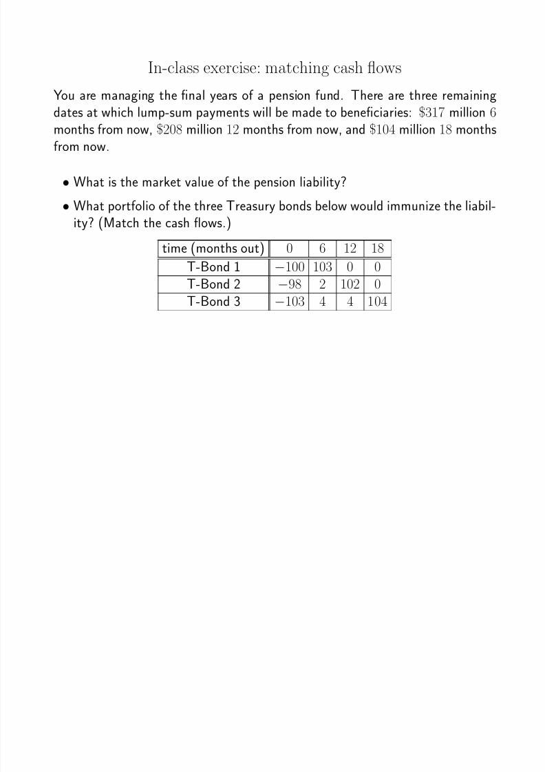
In-class exercise: matching cash flows

You are managing the final years of a pension fund. There are three remainingdates at which lump-sum payments will be made to beneficiaries: $317 million 6months from now, $208 million 12 months from now, and $104 million 18 monthsfrom now.

• What is the market value of the pension liability?

• What portfolio of the three Treasury bonds below would immunize the liabil-ity? (Match the cash flows.)

time (months out) 0 6 12 18

T-Bond 1 −100 103 0 0

T-Bond 2 −98 2 102 0T-Bond 3 −103 4 4 104



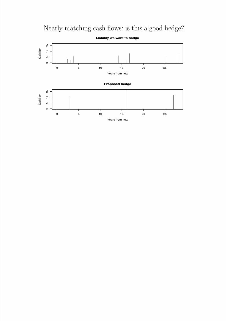
Nearly matching cash flows: is this a good hedge?

0 5 10 15 20 25

0

5

1 0

1 5

Liability we want to hedge

Years from now

C a s h f l o w

0 5 10 15 20 25

0

5

1 0

1 5

Proposed hedge

Years from now

C a s h f l o w



Nearly matching cash flows: a diagnostic tool

Intuitively, it seems like the proposed hedge might do well, but how can we getan objective measure of how well it will do? We can use the same tool as weused for intuition, namely, plotting the net amount at risk at each future date asa measure of our exposure to the forward rate.

For example, consider a liability of $100 a year from now with a present value

of $95, and $200 two years from now with a present value of $190. Then theexposure is the full present value $285 from now until a year from now, thepresent value $190 of the second cash flow only from one year from now untiltwo years from now, and $0 beyond two years.

Consider funding the liability with a portfolio that pays $298 one and one-half

years from now, with present value of $285. Then this investment has a riskexposure of $285 from now until one and one-half years out and $0 thereafter.The net exposure is the difference of the two, which is $0 from now until oneyear out, −$95 from one year out until one and one-half years out, $190 fromone and one-half years out until two years out, and $0 thereafter.



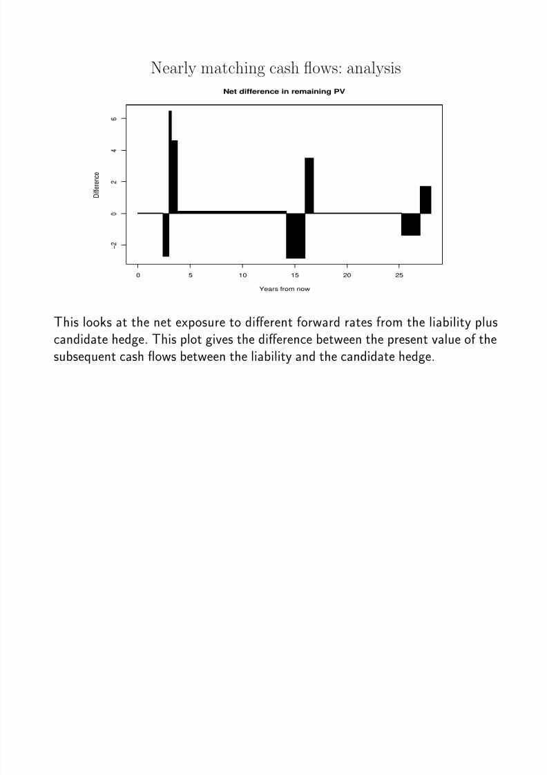
Nearly matching cash flows: analysis

0 5 10 15 20 25

− 2

0

2

4

6

Net difference in remaining PV

Years from now

D i f f e r e n c e

This looks at the net exposure to different forward rates from the liability pluscandidate hedge. This plot gives the difference between the present value of thesubsequent cash flows between the liability and the candidate hedge.



• Strict matching of cash flows: difference = 0

• Effective approximate hedge– total area between the difference and the axis is small

– areas above and below the axis are nearly matched in time

• Matched duration: total signed area is zero



Caution: fixed claims only

The exposure analysis only works (in this form) for nonrandom claims. Forexample, a bond fully indexed to the short rate has no exposure to shocks ininterest rates. The same is true of the Macauley duration defined below: theformula for duration assumes nonrandom claims and does not work for floating-rate bonds and more complex claims.



Duration

When there is a single source of interest rate risk, it is useful to think of our mea-sure of interest rate risk being the equivalent investment in a zero-coupon bondwith the same risk exposure. The traditional (Macauley) measure of durationcan be derived in a world in which there is a flat term structure that can moveup or down. With a flat term structure, a small change δ in the interest rategives an approximate proportional change in the value of a zero-coupon bondwith time-to-maturity T .

1/(1 + r + δ)T − 1/(1 + r)T

1/(1 + r)T ≈ −

δ

1 + rT

For a bond promising cash flows cs at each future time s,

P (r) =T

t=1

ct(1 + r)t

is the value of the bond. Then for a small change δ in the interest rate r , the

proportionate change in value is approximately



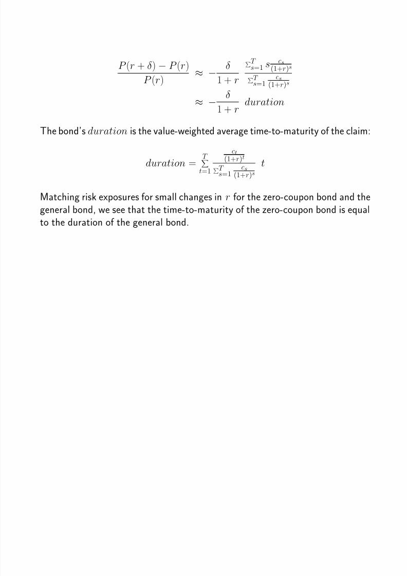
P (r + δ) − P (r)

P (r) ≈ −δ

1 + r

T s=1 s

cs

(1+r)s

T s=1

cs(1+r)s

≈ −δ

1 + rduration

The bond’s duration is the value-weighted average time-to-maturity of the claim:

duration =T

t=1

ct(1+r)t

T s=1

cs(1+r)s

t

Matching risk exposures for small changes in r for the zero-coupon bond and the

general bond, we see that the time-to-maturity of the zero-coupon bond is equalto the duration of the general bond.



Duration: some observations

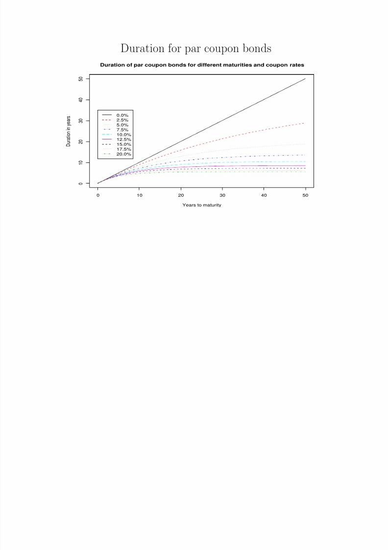
• The duration of a coupon bond or self-amortizing bond falls as rates rise.

• For near maturity coupon bonds, duration is close to time-to-maturity.

• For long maturity coupon bonds, duration is much less than time-to-maturity.

• As maturity approaches infinity, the duration of a par coupon bond approaches

1/r (exact with continuous coupon and compounding, (1+r/2)/r with semi-annual coupon and compounding)



Duration for par coupon bonds

0 10 20 30 40 50

0

1 0

2 0

3 0

4 0

5 0

Duration of par coupon bonds for different maturities and coupon rates

Years to maturity

D u r a t i o n i n y e a r s

0.0%2.5%

5.0%

7.5%

10.0%12.5%

15.0%

17.5%

20.0%



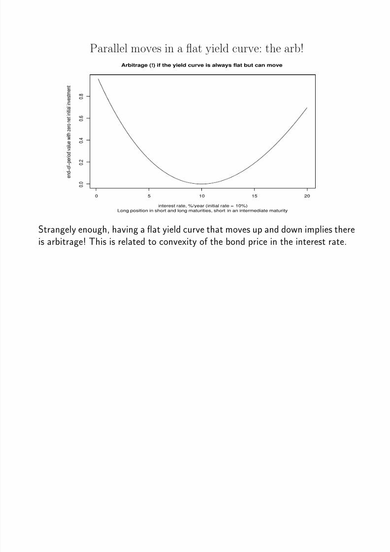
Parallel moves in a flat yield curve: the arb!

0 5 10 15 20

0 . 0

0 . 2

0 . 4

0 . 6

0 . 8

Arbitrage (!) if the yield curve is always flat but can move

Long position in short and long maturities, short in an intermediate maturityinterest rate, %/year (initial rate = 10%)

e n d − o f − p e r i o d v a l u e w i t h z e r o n e t i n i t i a l i n v e s t m e n t

Strangely enough, having a flat yield curve that moves up and down implies thereis arbitrage! This is related to convexity of the bond price in the interest rate.



Effective duration

Effective duration captures the good features of duration while addressing itslack of flexibility. The effective duration of an interest-sensitive security is thetime-to-maturity of the zero-coupon bond with the same interest sensitivity. If we are looking at nonrandom claims, the effective duration is equal to Macauleyduration. Effective duration can also be computed given different assumptionsabout interest rate shocks that do not hit all yields equally (which is good becauseshort rates move around more than long rates). Also, effective duration can becomputed for a variety of interest derivatives if we know how their prices dependinterest rates. Option pricing theory is an ideal tool for performing this analysis; inthe next lecture we will consider the use of option pricing tools in pricing interestderivatives. The rest of this lecture is devoted to a more traditional approach.



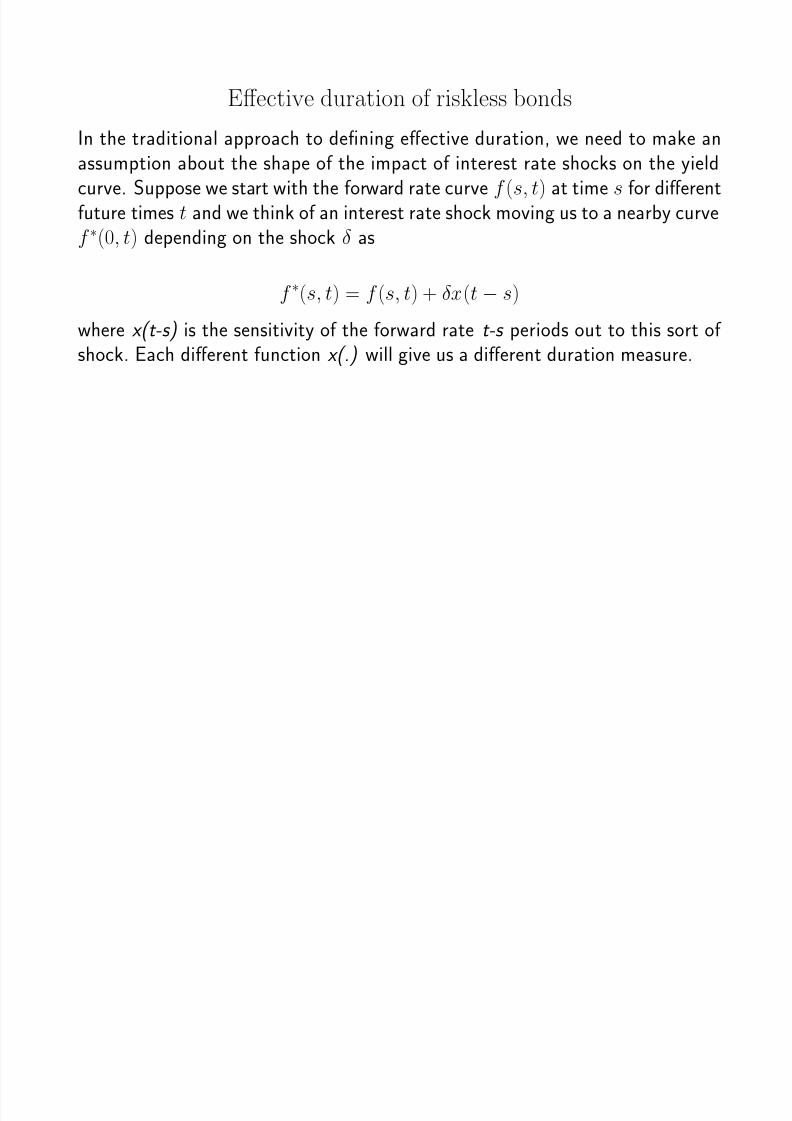
Effective duration of riskless bonds

In the traditional approach to defining effective duration, we need to make anassumption about the shape of the impact of interest rate shocks on the yieldcurve. Suppose we start with the forward rate curve f (s, t) at time s for differentfuture times t and we think of an interest rate shock moving us to a nearby curvef ∗(0, t) depending on the shock δ as

f ∗(s, t) = f (s, t) + δx(t − s)

where x(t-s) is the sensitivity of the forward rate t-s periods out to this sort of shock. Each different function x(.) will give us a different duration measure.



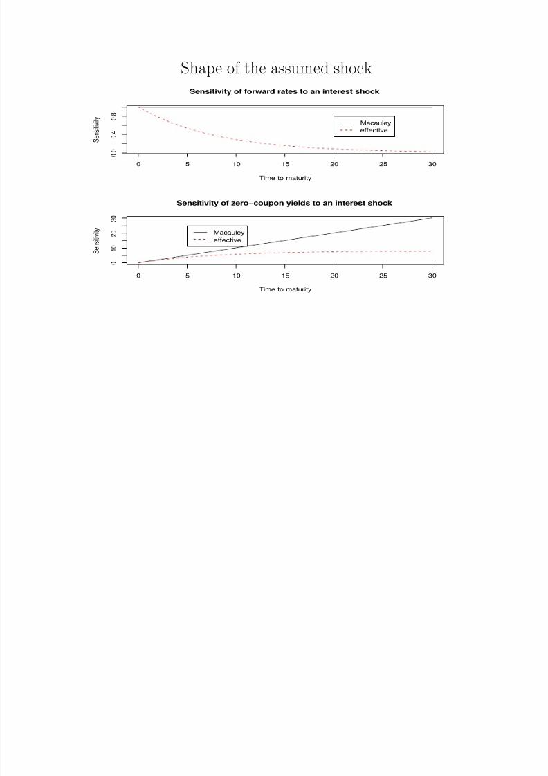
Effective duration: shape of the shock

Factor analysis of errors in predicting next-period bond yields suggests usingfactors corresponding coarsely to the level of the yield curve, the slope of theyield curve, and curvature of the yield curve. The factor corresponding to levelsexplains the lion’s share of the variance and has a sensitivity of the forwardprice to the shock that declines as time-to-maturity increases. According to theestimates in one paper of mine,1 the function x(t − s) = exp(−.125(t − s)) is agood fit for this dominant factor. The corresponding shock to zero-coupon yieldsis sens(t − s) = (1 − exp(−.125(t − s)))/.125, that is, the effective duration of a bond with cash flows ct at times t = 1, 2,...,T will have an effective durationthat solves

sens(duration) =

T s=1 sens(s)csD(0, s)

T

s=1 csD(0, s)

which is the same as the formula for Macauley duration except substituting y(s)for the impact s on both sides and using the general formula D(0, s) for thediscount factor. To solve for duration, it is useful to note that the log() (base e)is the inverse of exp(), and therefore duration = −log(1 − .125 ∗ sens)/.125.

1Dybvig, Philip H., Bond and Bond Option Pricing Based on the Current Term Structure, 1997, Mathematics of Derivative Securities, Michael A.

H. Dempster and Stanley Pliska, eds., Cambridge University Press.



Shape of the assumed shock

0 5 10 15 20 25 30

0 . 0

0 . 4

0 . 8

Sensitivity of forward rates to an interest shock

Time to maturity

S e n s i t i v i t y

Macauley

effective

0 5 10 15 20 25 30

0

1 0

2 0

3 0

Sensitivity of zero−coupon yields to an interest shock

Time to maturity

S e n s i t i v i t y Macauley

effective



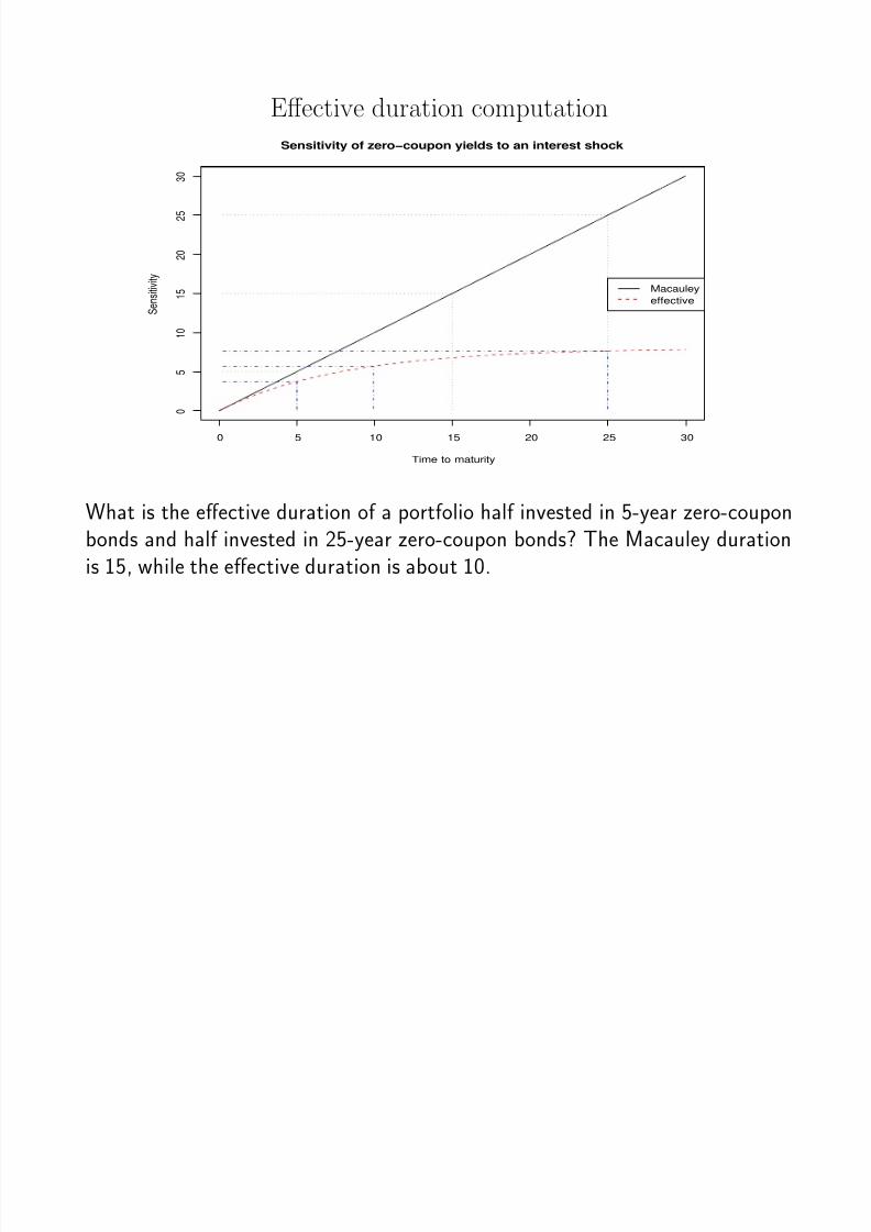
Effective duration computation

0 5 10 15 20 25 30

0

5

1 0

1 5

2 0

2 5

3 0

Sensitivity of zero−coupon yields to an interest shock

Time to maturity

S e

n s i t i v i t y

Macauley

effective

What is the effective duration of a portfolio half invested in 5-year zero-couponbonds and half invested in 25-year zero-coupon bonds? The Macauley durationis 15, while the effective duration is about 10.



In-class exercise: effective duration

Assuming the sensitivity of discount bond prices to a shock is given by sens(t −s) = (1 − exp(−.125(t − s)))/.125 (as we have been assuming), compute theMacauley duration and the effective duration of a bond which pays 3/4 of itsvalue at 30 years out and 1/4 of the value 10 years out. Either use the graphon the previous slide to obtain an approximate value, or use the formulas from acouple of slides back to perform a more exact computation.



Multiple duration measures

One interesting traditional extension to using duration is to use multiple durationmeasures and to assert that the risk exposure is matched if each of the durationmeasures is matched. Thus, we may have a separate duration measure for up-and-down movements in the whole yield curve, and for changes in the slope andcurvature of the yield curve as well. In practice, using multiple measures is useful(and can give a more realistic assessment of the risk in positions that are designed

to be neutral to a single duration measure). Often, using multiple measures isnot much different in its prescription than approximate matching of cash flowsas we have discussed earlier.

risk and exposure by apte

Documents