risk assessment framework for ballast water …in the ballast tank with the vessel’s journey...
TRANSCRIPT

AUGUST 2000
CENTRE FOR RESEARCH ON INTRODUCED MARINE PESTSTECHNICAL REPORT NO. 21
RISK ASSESSMENT FRAMEWORK FOR BALLAST WATER INTRODUCTIONS - VOLUME II
KEITH R.HAYES AND CHAD L.HEWITT

Hayes, Keith Robert. Risk assessment framework for ballast water introductions Volume II
Bibliography. Includes index. ISBN 0 643 06228 9.
1. Ballast water – Environmental aspects – Australia. 2. Discharge of ballast water – Environmental aspects – Australia. I. Hewitt, Chad L. (Chad LeRoi), 1960 - II. CSIRO. Division of Marine Research. III. Centre for Research on Introduced Marine Pests (Australia). IV. Title. (Series : Technical report (Centre for Research on Introduced Marine Pests (Australia)) ; no. 21). 363.72846

SUMMARY
This report provides a detailed description of the ballast-water risk assessment framework developed by the Centre for Research on Introduced Marine Pests (CRIMP), on behalf of the Australian Quarantine and Inspection Service (AQIS). The report also includes the preliminary results of a demonstration project designed to estimate the ballast water risk posed by Asterias amurensis and Gymnodinium catenatum for vessels arriving in Newcastle from selected ports in Japan.
The risk assessment framework is both modular and hierarchical, allowing increasingly accurate estimates of risk as more data is made available to the analyst. Risk estimates are made on a per vessel, per species basis, for the month in which the vessel intends to de-ballast in the recipient port. Ballast water risk is defined as
( ) ( ) ( ) ( )υψφω= p.p.p.pRisk species , where p(ω) is the probability that the donor port is infected with the species, p(φ) is the probability that the vessel becomes infected with this species, p(ψ) is the probability that the species survives the vessel’s journey and p(υ) is the probability that the species will survive in the recipient port.
The probability that the donor port is infected p(ω) should be determined via a survey – ideally one designed to allow an objective estimate of the probability of Type II error (ie the species is present but undetected). As an interim measure, the infection status of the donor port bioregion can be used as a surrogate for international ports that have not been surveyed.
A fault tree analysis identifies ten infection scenarios that are mutually exclusive for most species. The assessment framework uses these infection scenarios to quantify the probability of vessel infection p(φ). For large complex ports it will be difficult to accurately quantify the probability of infection because third party vessels will influence the vertical and horizontal distribution of target species, and the ballast withdrawal envelope described by the target vessel. For species that exhibit resistant or diapause life-stages, however, this is a very important component of the assessment because substantial risk reductions may not be achieved elsewhere in the assessment framework.
The probability of journey survival p(ψ) is estimated by comparing the species life expectancy in the ballast tank with the vessel’s journey duration. Uncertainty regarding the species life expectancy is expressed through a probability distribution. Birth-death models were avoided in this context because it is very difficult to estimate the initial inoculum size on any given ballast event. By contrast it is much easier to measure the life expectancy using on-board sampling.
The probability of survival in the recipient port p(υ) is estimated by comparing the species temperature and salinity tolerances with the probability distribution of salinity and temperature in the recipient port. The recipient port is divided in environmental sub-units for the purposes of this analysis. Ideally the temperature and salinity extremes of each environmental sub-unit are characterised by monthly extreme value distributions. The risk assessment framework allows for kernel density estimates and sample distribution functions, however, if there is insufficient data to fit an extreme value model.
The framework described in this report represents a significant step towards quantified estimates of ballast water risk. The framework should, however, be considered as ‘work-in-progress’. There is considerable scope for continued development of the framework, particularly in the vessel infection and journey survival components. In this context we recommend:
• journey survival models are specifically developed for each target species;
• vessel infection models are specified and tested in port environments to ascertain the accuracy of the techniques described in this report, and the significance of third-party vessel activity;
• port infection models are developed that acknowledge the probability of Type II error and allow the probability of infection to vary as a function of time elapsed since the last port survey;
• a pilot analysis of the efficacy of the environment HAZOP techniques described in this report; and,
• that the predictions of the risk assessment framework are routinely checked as part on an on-going program of testing and improvement.
We also make the following recommendations to assist in the continued development of an international risk-assessed ballast management regime:
• national and international species-reporting systems should be developed that emulate the OIE and FAO pest-reporting system, and assignation of Pest Free Areas. A national approach for aquaculture disease is currently being developed in Australia via AQUAPLAN. This approach should be extended to include marine pests;
• uniform ballast reporting forms be adopted internationally, and archived, to assist in the assessment of the risks associated with ballast water carry over; and,
• gene probes are developed for target species in order to reduce the time and cost of identifying target species in ballast water samples.

ACKNOWLEDGMENTS
This work is partially funded by the Australian Quarantine and Inspection Service, through the Strategic Ballast Water Research Program (Contract No. AQIS 003/96).
Mr. Andrew Dobbie (Hobart Ports Corporation) and Mr. Andrew Walsh (Australian Oceanographic Data Centre) kindly supplied environmental data for the ports of Hobart and Sydney.
Maps of the bioregion distribution of Asterias amurensis and Carcinus maenas, the IMCRA bioregions of Australia, and the port of Newcastle are reproduced from the CRIMP invasion database being developed by Dr. Chad Hewitt.

CONTENTS
SUMMARY ................................................................................................................................................ 1
ACKNOWLEDGMENTS ......................................................................................................................... 3
CONTENTS................................................................................................................................................ 4
LIST OF SYMBOLS ................................................................................................................................. 6
1 INTRODUCTION TO VOLUME II................................................................................................ 1
1.1 BACKGROUND ................................................................................................................................. 1 1.2 THE STRUCTURE OF THE REPORT..................................................................................................... 2 1.3 NOTATION ....................................................................................................................................... 2
2 OVERVIEW OF THE RISK ASSESSMENT................................................................................. 3
p(ω) ..................................................................................................................................................... 3 p(φ) ...................................................................................................................................................... 4 p(ψ) ..................................................................................................................................................... 4 p(υ)...................................................................................................................................................... 5
3 DEMONSTRATION PROJECT ..................................................................................................... 7
3.1 DATABASE STRUCTURE ................................................................................................................... 7 3.2 RISK ASSESSMENT METHODOLOGY............................................................................................... 12
Level 0 ............................................................................................................................................... 12 Level 1 ............................................................................................................................................... 12 Level 2 ............................................................................................................................................... 16 Level 3 ............................................................................................................................................... 18
3.3 RESULTS ........................................................................................................................................ 20 Level 0 ............................................................................................................................................... 20 Level 1 ............................................................................................................................................... 22 Level 2 ............................................................................................................................................... 22 Level 3 ............................................................................................................................................... 25
4 DATA COLLECTION – MODULE 0 ........................................................................................... 27
4.1 VESSEL-VISIT DATA ....................................................................................................................... 27 4.2 INFORMATION HELD IN DATABASES............................................................................................... 28
5 PORT INFECTION STATUS – MODULE I................................................................................ 33
5.1 BACKGROUND ISSUES .................................................................................................................... 33 5.2 PORT SURVEYS .............................................................................................................................. 34
Port survey techniques ...................................................................................................................... 34 Probability of Type II errors ............................................................................................................. 36
5.3 DONOR-PORT INFECTION STATUS................................................................................................... 40 5.4 RECIPIENT-PORT INFECTION STATUS.............................................................................................. 46 5.5 FUTURE DEVELOPMENTS ............................................................................................................... 46
6 PORT ENVIRONMENTS – MODULE II .................................................................................... 49
6.1 MEASURING ENVIRONMENTAL SIMILARITY ................................................................................... 49 6.2 TOLERANCE TEST........................................................................................................................... 51 6.3 PROBABILITY OF SURVIVAL ........................................................................................................... 52
Organism tolerances ......................................................................................................................... 52 Environmental characteristics........................................................................................................... 56 Parameter considerations ................................................................................................................. 72 Multi-variate considerations ............................................................................................................. 72 Environmental sub-units.................................................................................................................... 74

7 INFECTION SCENARIOS (MODULE III) ................................................................................. 77
7.1 WATER COLUMN ........................................................................................................................... 78 Planktonic ......................................................................................................................................... 78 Nuestonic........................................................................................................................................... 78 Vertical Migrator .............................................................................................................................. 80
7.2 SOFT-SUBSTRATE SOURCES ........................................................................................................... 81 Tychoplankton................................................................................................................................... 82 Vertical Migrator .............................................................................................................................. 95
7.3 HARD-SUBSTRATE SOURCES.......................................................................................................... 96 Tychoplankton................................................................................................................................... 96 Vertical Migrator ............................................................................................................................ 100
7.4 EPIPHYTE SOURCES ..................................................................................................................... 100 Tychoplankton................................................................................................................................. 100 Vertical Migrator ............................................................................................................................ 101 Floating Detached........................................................................................................................... 101
7.5 OTHER INFECTION SCENARIOS..................................................................................................... 101
8 JOURNEY SURVIVAL (MODULE IV)..................................................................................... 103
8.1 COMPETENCY TEST...................................................................................................................... 103 8.2 JOURNEY SURVIVORSHIP ............................................................................................................. 104 8.3 BALLAST PUMP EFFECTS.............................................................................................................. 106 8.4 MANAGEMENT STRATEGIES......................................................................................................... 107
9 INDUCTIVE HAZARD ASSESSMENT..................................................................................... 109
9.1 ENVIRONMENTAL DISTRIBUTION FUNCTIONS ............................................................................. 109 9.2 PORT AND VESSEL BASED HAZOP ANALYSIS ............................................................................ 110
What is HAZOP?............................................................................................................................. 110 HAZOP for natural port processes ................................................................................................. 114 HAZOP for berthing and ballasting processes ............................................................................... 114 HAZOP for port engineering activity.............................................................................................. 116
10 DISCUSSION AND RECOMMENDATIONS ........................................................................... 119
REFERENCES ...................................................................................................................................... 123
APPENDIX A SAMPLE INCLUSION PROBABILITY................................................................. 131
A1 VISUAL SURVEY IN LOW VISIBILITY............................................................................................. 132 A2 BENTHIC TRAWLS AND QUADRATS .............................................................................................. 134 A3 VISUAL SURVEY IN GOOD VISIBILITY........................................................................................... 135
APPENDIX B 2O DISTRIBUTION FUNCTIONS ........................................................................... 137
APPENDIX C KERNEL DENSITY ESTIMATORS....................................................................... 139
APPENDIX D FITTING EXTREME VALUE DISTRIBUTIONS................................................. 141
D1 NON-PARAMETRIC TECHNIQUES.................................................................................................. 141 D2 PARAMETER ESTIMATES .............................................................................................................. 142 D3 CORRELOGRAMS ......................................................................................................................... 143
APPENDIX E DEMONSTRATION PROJECT CODE .................................................................. 144

LIST OF SYMBOLS
τcr Critical shear-stress
τ0 Shear-stress at the sea-bed
T Excess shear-stress parameter
θcr Critical shields parameter
ρ Density of seawater
ρs Density of particle
s Specific weight
g Acceleration due to gravity
ws Particle sinking velocity
ε Wall thickness (dinoflagellate cyst)
m1 Excess mass per unit area of the phragma (dinoflagellate cyst)
µ Absolute viscosity
υ Kinematic viscosity
r Particle radius
D* Particle parameter
D50 Median particle diameter
Ds Particle diameter of bed material
CD Drag coefficient
C100 Drag coefficient at 1m above the sea-bed
u, w, v Orthogonal components of velocity vector
U, W, V Non-dimensional velocity vectors
x, y, z Orthogonal spatial components
X, Y, Z Non-dimensional spatial components
t Time
P Non-dimensional pumping time
p Ambient current
u Time-mean flow (in the dominant direction)

ú Turbulent deviation (in the dominant direction)
u* Friction velocity
u100 Velocity at 1m above the sea-bed (in the dominant direction)
u0 Efflux velocity at the face of the propeller
ux,,r Axial velocity at a point x aft and r below the propeller axis
cz Particle concentration at a distance z above the sea-bed
ca Particle concentration at a reference distance a above the sea-bed
c0 Static bed concentration
cb Particle concentration in the bed-load layer
Hp Distance between the propeller axis and the sea-bed
c Distance between the propeller tip and the sea-bed
θ Jet expansion angle (degrees)
zmax Maximum depth of propeller induced scour
D0 Initial width of propeller jet
Dp Propeller diameter
h Total water depth
n Propeller revolutions per second
KT Propeller thrust coefficient
α Boundary conditions coefficient
A Rudder effect coefficient
a Acceleration of fluid
V Volume of fluid
Fa Force of acceleration
Fp Dislodgment force
q1, q2, q3 Dislodgment coefficients
Fd Drag Force
Fl Lift force
Ca Added mass coefficient
Cm Inertia coefficient

βd Velocity exponent of drag
βl Velocity exponent of lift
Sd, pr Shape coefficient of drag
Sl, pl Shape coefficient of lift
Apr Profile area
A, pl Planform area

Introduction to Volume II
CRIMP Technical Report Number 21
1
1 INTRODUCTION TO VOLUME II
1.1 Background This document is Volume II of a three-volume report that describes a framework for quantitative ballast-water risk assessment. Volume I (Hayes and Hewitt, 1998) includes background material and provides a summary description of the analysis and data requirements at each level of the framework. Much of this material, however, is superseded by this document. Volume III (Hayes, 1998) examines the use of Bayesian statistical techniques in ecological risk assessment.
The purpose of this document is to provide:
• a detailed description of the analysis required at each level of the framework, supported by theoretical constructs where appropriate; and,
• a non-technical description of the risk assessment demonstration project developed for a selected group of ports in SE Australia and Japan.
The scope, objectives and structure of the framework are outlined in Volume I. The reader is referred to that document for details. At this point, however, it is worth emphasising that:
• the framework is species-specific and is predicated on a target list of species a priori considered as marine pests;
• the risk-assessment endpoint is the probability of survival in the recipient port - the framework does not currently address the likelihood of establishment (and subsequent adverse environmental impact) of non-native species;
• the framework is concerned with spread of non-indigenous species through ship’s ballast water and sediment discharges - it does not address port contamination through the natural processes of dispersal and colonisation via range expansion; and,
• the framework does not current address hull fouling - similarly the assessment makes no allowance for crevicolous species that actively seek cavities on a vessel’s hull such as seachests.
The risk assessment is conducted on a vessel-by-vessel basis and provides a species-specific estimate of risk defined as
( ) ( ) ( ) ( )υψφω ppppRiskspecies ⋅⋅⋅= [1.1] where p(ω) is the probability that the donor port is infected with the species, p(φ) is the probability that the vessel becomes infected with this species, p(ψ) is the probability that the species survives the vessel’s journey and p(υ) is the probability that the species will survive in the recipient port. Each of these elements are discussed in detail in this report. Note that this equation has been developed from, and supersedes, that given in Hayes and Hewitt (1998).

Introduction to Volume II
CRIMP Technical Report Number 21
2
1.2 The structure of the report The first half of this report (chapters 1 to 3) provides a non-technical description of the risk assessment framework, data requirements and the results of the demonstration project. The second half of the report (chapters 4 to 8) provides a detailed technical description of the modules used by the framework, and the analysis used (or envisaged) at each level of the risk assessment. Chapter 2 provides a summary overview of the risk assessment, describing the analysis that takes place at each level, or tier, of the assessment framework. Chapter 3 describes the demonstration project used to illustrate the risk assessment, and its data needs, up to level 3. This chapter illustrates the results of the analysis for Asterias amurensis and Gymnodinium catenatum.
Chapter 4 describes Module 0, which collects the data needed to run the risk assessment. Chapter 5 describes Module I, which is used to determine the probability p(ω) that the donor port is infected with any of the target species. Chapter 6 describes Module II, which determines the salinity and temperature characteristics of the recipient and donor ports, and inter alia the probability p(υ) that the target species will survive in the recipient port. Chapter 7 discusses Module III, which determines p(φ) - the probability that the vessel becomes infected with a target species. Chapter 8 discusses Module IV, which calculates the probability p(ψ) that the target species will survive the vessel’s journey.
The penultimate chapter (chapter 9) describes an inductive hazard analysis designed to assist Modules II and III. Chapter 10 provides discussion and recommendations. Additional mathematical details are included in Appendices A to D. The demonstration project code is reproduced in Appendix E.
1.3 Notation The notation used in this document is that same as that used in Volume III, unless otherwise indicated. Random variables are represented by capitals, such as X or Y. Values taken by these variables are represented by x or y. Pr(A) denotes the probability of a particular outcome or event. Letters, text or symbols will be used in the parenthesis to refer to the outcome or event in question. If this probability is conditional upon a second event or outcome, then this is denoted Pr(A/ B).
A probability mass or density function assigns probability to values of a discrete or continuous variable, and is denoted f(x). In both cases F(x) signifies the cumulative distribution function. The joint probability distribution of two or more variables is denoted p(x, y). The terms ‘density’ and ‘distribution’ are used interchangeably. The asymptotic distribution function of an extreme value is denoted G(x). The corresponding probability density function is written g(x).
The parameter(s) that characterise a probability density function are generically denoted by Greek symbols. It is common therefore to write p(y/θ) to signify that the probability function is conditional on the parameters of the distribution. The probability of the parameter given the data is written p(θ/y). The mean of a probability function (or population) is written µ, the standard deviation σ. The sample mean and standard deviation are written x and s respectively. A circumflex denotes parameter estimates of a distribution. For example
x=µ signifies that the sample mean is being used as an estimate of the population mean

Overview of the Risk Assessment
CRIMP Technical Report Number 21
3
2 OVERVIEW OF THE RISK ASSESSMENT
The ballast-water invasion cycle (like all bio-invasions) is a complex process of stochastic events operating at a vector-, species- and site-specific level. It is difficult to predict which species are arriving, and when and where they will be successful.
Two approaches to ballast-water risk assessment have emerged in response to this complexity. The first advocates an approach based entirely on the environmental similarity between donor and recipient regions, and does not therefore require any species information. The second advocates a species-specific approach, but must therefore select a set of target-species on which to perform the assessment. It is important to emphasise that these two approaches are not mutually exclusive – the strengths of one complement the weaknesses of the other.
The risk-assessment framework recommended in this document includes both approaches, and has the following characteristics:
• it provides a simple measure of ballast-water hazard based on the environmental similarity of donor bioregion and recipient ports;
• it allows a vector-, species- and site-specific assessment of ballast-water risk to be made at several levels of complexity, depending on the availability of vector, species and site information; and,
• the framework implicitly assumes that all vessels are high-risk and maintains a conservative stance in the face of uncertainty.
The framework is divided into six tiers or levels (0 to 5). Each level attempts to provide an increasingly accurate estimate of risk by reducing uncertainty. In most cases this is achieved by collecting information that allows site- and species-specific models to be run. The framework therefore offers demonstrable risk-reduction benefits for additional data costs, and is consistent with the precautionary principle (Fairbrother and Bennet, 1999).
The risk-assessment endpoint is the survival of target-species in Australian ports, allowing ballast-water risk to be defined as
( ) ( ) ( ) ( )υψφω ppppRiskspecies ⋅⋅⋅= , [1.1]
where p(ω) is the probability that the donor port is infected with the target-species, p(φ) is the probability that the vessel becomes infected with this species, p(ψ) is the probability that the species survives the vessel’s journey, and p(υ) is the probability that the species will survive in the recipient port.
p(ω) The probability that the donor port (or bioregion) is infected p(ω) is fundamental to the risk assessment and is used at all levels of the analysis. Ideally p(ω) is estimated through port-surveys. If a target species is detected by a survey then p(ω) = 1.0 until the population is eradicated or becomes demonstrably extinct. If a target species is not detected, then p(ω) is function of the probability of a Type II error and the probability that the species is able to

Introduction to Volume II
CRIMP Technical Report Number 21
4
survive in the port p(υ). If neither of these can be calculated, it is only safe to assume p(ω) = 1.0, until data is collected that allows p(υ) to be calculated, or until another survey is conducted.
If a port has not been surveyed then p(ω) is inferred from the infection status of the bioregion. If the target-species is recorded anywhere in the bioregion, the bioregion is assumed to be infected, and all unsurveyed donor ports within that region similarly infected unless the species cannot survive in the port. If the bioregion is not infected, ie the species has not been recorded anywhere in the region, then p(ω) is set equal to p(υ) multiplied by some small probability to reflect uncertainty regarding the infection status of the port. If p(υ) cannot be calculated then the probability of infection is set equal to the same small probability used before to reflect uncertainty about the true infection status of the port. Note how this approach applies risk penalties to unsurveyed ports once a target species has been recorded in a bioregion, and requires information to calculate p(υ) of all ports.
The probability that the vessel is infected p(φ) is introduced at level 1. At this level the analysis is quite simple. More sophisticated techniques, however, are envisaged at levels 4 and 5. The framework has identified ten life-stage specific vessel-infection scenarios. Risk-assessment models are available for most of these scenarios, although considerable uncertainty surrounds the importance of vertical migration and the effect of vessel movements on the vertical concentration profile of a port. In most cases, however, the risk assessment will be hindered by lack of data rather than theoretical understanding. Again in this situation the framework maintains a conservative stance, assuming p(φ) = 1.0 if there are insufficient data to run the risk assessment models. Inductive HAZOP techniques could be used here to test model assumptions against the reality of vessel berthing and ballasting processes.
The framework also identified a number of less tractable infection scenarios, including ballast-water carry-over, ballast-tank populations and third-party infections. The latter cannot be addressed without a very detailed analysis, such as that envisaged at level 5 of the framework. In the meantime p(φ) is set to a minimum of 0.05 to allow for this possibility. Species capable of establishing ballast-tank populations will be flagged by the assessment. The risks associated with ballast-water carry-over cannot be addressed until journey-survival models are developed, and ballast-reporting mechanisms are adopted internationally.
p(ψ) The probability that a species will survive the vessel’s journey p(ψ) is introduced at level 2 of the framework. Most studies to date show the abundance of most species declining exponentially with time during the vessel’s journey. By re-specifying this process in terms of a random variable T – the life-expectancy of the species in a ballast-tank - it is possible to model the probability of journey survival p(ψ) without knowing the initial abundance at the start of the journey.
If the survival model is specified in Bayesian terms it can be updated using ballast samples taken at the recipient port, but only where species are recorded as present. Thus in the first instance the distribution and parameters of T must be determined by field studies onboard a vessel during its journey. The cost of these studies could be reduced if genetic techniques were used to identify and estimate the abundance of target-species in ballast-water samples.

Overview of the Risk Assessment
CRIMP Technical Report Number 21
5
p(υ) The probability that a species will survive in the recipient port p(υ) is introduced at level 3 of the framework. The probability of survival is a function of the species tolerance relative to key environmental parameters (temperature and salinity in the first instance), and values that these parameters take in the port. There are a number of ways to calculate p(υ), we recommend that the following approaches be adopted, in order of preference:
• use an Extreme Value (EV) distribution and its return period to calculate the probability that the species’ tolerance is exceeded during an exposure period equal to that used to calculate the tolerable limits;
• fit a kernel density estimate to the extreme values of the parameter, and compare this to the species’ tolerances; or
• fit a second order1 sample distribution function to the parameter values, and compare this to the species’ tolerances.
The first approach will require a time-series analysis and at least 5 years of data for each month. The second approach requires at least one year of data collected daily for each month. The third approach requires at least 1 year of data, collected at some interval in each month. The final approach can be used when data is scarce but will provide increasingly accurate probability estimates as more data is used.
To calculate the probability of survival, the analyst must determine the environmental tolerances of the species and life-stages concerned. The analyst should be aware that these tolerances are influenced by a variety of factors, and are intimately linked to the exposure period used when they were calculated. The analyst should check the exposure limit and all other relevant factors when using limits that are published in the literature. Ideally the tolerances of a species will be represented by a probability distribution to allow for the uncertainty associated with confounding factors. Alternatively the analyst can adjust the lethal limit by a safety factor to allow for uncertainty when extrapolating from the laboratory to the field.
The environmental sub-units within a port must be identified prior to a level 3 assessment. Environmental data should be collected for each of these sub-units, and from at least two points in the water column. Inductive HAZOP procedures can be used to test the extent to which the port environment is adequately described by any existing information. The environmental sub-units will initially be identified using local knowledge of the port environment. Ultimately, however, these units should be objectively identified using multi-variate cluster and ordination analyses of environmental data.
1 A sample distribution function is an estimate of the parameter’s variability. A second-order function reflects the analyst’s uncertainty in this estimate.

.

Demonstration Project
CRIMP Technical Report Number 21
7
3 DEMONSTRATION PROJECT
The demonstration project provides a test-bed for the risk assessment framework and illustrates the risk reductions achieved at each level of the assessment framework. The project calculates the hazard/risk posed by Asterias amurensis and Gymnodinium catenatum for vessels arriving in Newcastle from selected ports in Japan. The vessel characteristics used throughout the demonstration project are those of the BHP’s MV Iron. The demonstration project is complete to level 3 and includes a bayesian journey-survival model for the larval life-stages of Asterias (Hayes, 1998). The hazard and risk assessment algorithms are written in Visual Basic for Applications (VBA), and the databases are held in Microsoft Excel.
3.1 Database structure The risk assessment framework uses four databases - port, vessel, species and ballast details (from the archive). The entities and attributes of these databases are illustrated in Figures 3.1 to 3.4 respectively. Attributes in bold text represent the data items that are used by the project up to and including level 3. The project archives the ballast details, collected by Module 0, each time the risk assessment is run. It is important to note that the databases are not finalised –attributes may be added or removed if the demonstration project is developed to levels 4 or 5.
The port database reflects the three levels of geographical resolution built into the risk assessment framework, namely bioregion, port and environmental sub-unit, and illustrates the one-to-many relationship between each. Most of the port attributes are static, and need only be updated if the port infrastructure is substantially modified – for example if a new berth is constructed. The environmental attributes, such as temperature and salinity, may need to be updated, however, as additional information is gathered.
The species database reflects a similar one-to-many relationship between a species and its life-stages. Again most of this information need only be entered once, and only updated if new information comes to light that significantly alters any of the attributes.
The vessel database is largely comprised of technical information that is common to all vessels. The number of ballast tanks, intakes, sieves and thrusters, however, may vary from vessel to vessel and are thus recorded as separate entities. Again most of the vessel attributes need only be entered once, with the important exception of the date of last:
• dry-dock or in water hull and propeller scrub ;
• sea-chest clean and service; and,
• service of the ballast water sea suction strainer.
The date since the ballast water sea suction strainer was last serviced is particularly important because this will determine the effective size of the strainer and thus the largest organisms that can enter the tank.

Demonstration Project
CRIMP Technical Report Number 21
8
Figure 3.1 Port database used by the demonstration project
BRG
_ID
: Aut
onum
ber
BR
G_N
ame:
Tex
tBR
G_N
umbe
r: In
tege
rB
RG
_Sub
regi
on: T
ext
BR
G_T
arge
tPes
t: B
inar
y (x
9)BR
G_T
empD
ataC
ode:
Tex
tB
RG
_Max
Tem
p: S
ingl
e (x
12)
BR
G_M
inTe
mp:
Sin
gle
(x12
)B
RG
_Sal
Dat
aCod
e: T
ext
BR
G_M
axSa
l: Si
ngle
(x12
)B
RG
_Min
Sal:
Sing
le (x
12)
Bior
egio
ns
POR
_ID
: Aut
onum
ber
BR
G_N
ame:
Tex
tBR
G_N
umbe
r: In
tege
rBR
G_S
ubre
gion
: Tex
tBR
G_S
ubzo
ne:
BRG
_IM
CR
A: T
ext (
3)PO
R_F
AO: T
ext (
1) ?
?PO
R_S
tate
: Tex
tPO
R_C
ount
ry: T
ext
POR
_Nam
e: T
ext
POR
_AQ
IS 1
st P
ort:
Inte
ger
POR
_Ope
n: T
ext (
1)PO
R_R
iver
: Tex
tPO
R_E
quiv
alen
t riv
er: T
ext
POR
_ Id
ent:
Text
POR
_Lat
itude
: Sin
gle
POR
_Lon
gitu
de: S
ingl
ePO
R_H
abita
t: Bi
nary
POR
_LLZ
: Tex
tPO
R_B
erth
Cou
nt: I
nteg
erPO
R_T
ugC
ount
: Int
eger
POR
_Max
Dra
ft: S
ingl
ePO
R_R
esus
p: T
ext
POR
_ Ex
ports
: Tex
tPO
R_I
mpo
rts: T
ext
POR
_Tid
alR
ange
: Sin
gle
POR
_Tid
alFl
ow: S
ingl
ePO
R_W
inds
:Tex
tPO
R_S
urve
yed:
Text
POR
_Tar
getP
est:S
ingl
e (x
9)PO
R_T
empD
ataC
ode:
Tex
tPO
R_M
axTe
mp:
Sin
gle
(x12
)PO
R_M
inTe
mp:
Sin
gle
(x12
)PO
R_S
alD
ataC
ode:
text
POR
_Max
Sal:
Sing
le (x
12)
POR
_Min
Sal:
Sing
le (x
12)
POR
_Min
Am
bCur
rent
: Sin
gle
Ports
ESU
_ID
: Aut
onum
ber
CTY
_Nam
e: T
ext
POR
_Nam
e: T
ext
POR_
Iden
t: Te
xtES
U_I
dent
: Int
eger
ESU
_Nam
e: T
ext
ESU
_Tem
pDat
aCod
e: T
ext
ESU_
Max
Tem
p: S
ingl
e (x
12)
ESU
_Min
Tem
p: S
ingl
e (x
12)
ESU
_Sal
Dat
aCod
e: T
ext
ESU_
Max
Sal:
Sing
le (x
12)
ESU
_Min
Sal:
Sing
le (x
12)
Por
tEnv
ironm
enta
lSub
Uni
ts
1M
1M
1M
TUG
_ID
: Aut
onum
ber
CTY
_Nam
e: T
ext
PO
R_N
ame:
Tex
tTU
G_N
ame:
Tex
tTU
G_B
olla
rdP
ull:
Sing
leTU
G_P
ower
: Sin
gle
Por
tTug
s
BER
_ID
: Aut
onum
ber
CTY
_Nam
e: T
ext
POR
_Nam
e: T
ext
BER
_Nam
e: T
ext
BER
_Ide
nt: T
ext
ESU
_Ide
nt: I
nteg
erE
SU_#
: Int
eger
??B
ER_L
engt
h: S
ingl
eB
ER_M
inD
epth
: Sin
gle
Por
tBer
ths
1M

Demonstration Project
CRIMP Technical Report Number 21
9
Figure 3.2 Species database used by the demonstration project
SPS_
ID: A
uton
umbe
r
TXA_
ID: L
ong
inte
ger
SPS_
Latin
Nam
e: T
ext
SPS_
Com
mon
Nam
e: T
ext
SPS_
Min
Tem
pTol
: Sin
gle
SPS_
Max
Tem
pTol
: Sin
gle
SPS_
Min
SalT
ol: S
ingl
eSP
S_M
axSa
lTol
: Sin
gle
Spec
ies
SLS_
ID: A
uton
umbe
r
TXA_
ID: L
ong
inte
ger
SPS_
Latin
Nam
e: T
ext
SLS_
Com
mon
Nam
e: T
ext
SLS_
Hab
itat:
Text
SLS_
Min
Dur
atio
n: S
ingl
eSL
S_M
eanD
urat
ion:
Sin
gle
SLS_
Max
Dur
atio
n: S
ingl
eSL
S_M
inDi
amet
er: S
ingl
eSL
S_M
eanD
iam
eter
: Sin
gle
SLS_
Max
Dia
met
er: S
ingl
eSL
S_M
inD
epth
: Sin
gle
SLS_
Max
Dep
th: S
ingl
eSL
S_Te
mpT
olCo
de: T
ext
SLS_
Min
Tem
pTol
: Sin
gle
SLS_
Max
Tem
pTol
: Sin
gle
SLS_
SalT
olC
ode:
Tex
tSL
S_M
inSa
lTol
: Sin
gle
SLS_
Max
SalT
ol: S
ingl
eSL
S_Ha
bita
tCod
e: B
inar
y (x
4)SL
S_In
fect
ionC
ode:
Bin
ary
(x5)
SLS_
Wat
ColR
esN
: Bin
ary
(x12
)SL
S_W
atCo
lRes
S: B
inar
y (x
12)
SLS_
Min
Den
sity
: Sin
gle
SLS_
Mea
nDen
sity
: Sin
gle
SLS_
Max
Den
sity
: Sin
gle
SLS_
EnvC
ues:
Tex
t (x9
)SL
S_JS
Mod
elTy
pe: T
ext
SLS_
JSM
odel
Para
s: S
ingl
e
Spec
iesL
ifeSt
ages
1M

Demonstration Project
CRIMP Technical Report Number 21
10
Figure 3.3 Vessel database used by the demonstration project
VES_
ID: A
uton
umbe
r
Vess
el
VES_
Nam
e: T
ext
VES_
Dat
eBui
lt: D
ate
VES_
Flag
: Tex
tVE
S_C
allS
ign:
Tex
tVE
S_IM
ON
um: L
ong
inte
ger
VES_
Ow
ner/M
anag
er: T
ext
VES_
Ope
rato
r/Age
nt: T
ext
VES_
Com
mun
icat
ion:
Tex
tVE
S_D
eckV
olta
ge: S
ingl
eVE
S_Ty
pe/C
lass
: Tex
tVE
S_Le
ngth
: Sin
gle
VES_
Beam
: Sin
gle
VES_
Max
Dra
ft: S
ingl
eVE
S_G
RT:
Sin
gle
VES_
DW
T: S
ingl
eVE
S_To
talB
allC
ap: S
ingl
eVE
S_B
allT
ankC
ount
: Int
eger
VES_
Num
BallI
ntak
es: I
nteg
erVE
S_N
umB
allS
trai
ner:
Inte
ger
VES_
BallP
umpT
ype:
Tex
tVE
S_M
axPu
mpR
ate:
Sin
gle
VES_
Num
SeaC
hest
s: In
tege
rVE
S_M
axEn
gine
Pow
er: S
ingl
eVE
S_M
axSh
aftR
PS: S
ingl
eVE
S_N
umPr
op: I
nteg
erVE
S_Pr
opD
iam
eter
: Sin
gle
VES_
Prop
Pitc
h: S
ingl
eVE
S_Pr
opTy
pe: T
ext
VES_
Prop
Axis
ToKe
el: S
ingl
eVE
S_Pr
opH
ubD
iam
eter
: Sin
gle
VES_
Prop
Thru
stC
oeff:
Sin
gle
VES_
Num
Thru
ster
s: In
tege
rVE
S_D
ateL
astD
ryD
ock:
Dat
eVE
S_Lo
catio
nLas
tDry
Doc
k: T
ext
VES_
Antif
oula
nt: T
ext
VES_
Dat
eLas
tHul
lScr
ub: D
ate
VES_
Dat
eLas
tPro
pScr
ub: D
ate
VES_
Dat
eLas
tChe
stSc
rub:
Dat
eVE
S_Sa
mpl
ingL
imita
tions
: Tex
tVE
S_Ba
llExc
hang
eLim
its: T
ext
VES_
Car
goTy
pes:
Tex
tVE
S_Ba
llMan
Plan
: Bin
ary
VES_
BallL
og: B
inar
yVE
S_C
ompl
ianc
eHis
t: Te
xt
VBI_
ID: A
uton
umbe
r
VES_
Nam
e: T
ext
VES_
IMO
: Tex
tVB
I_Ba
llInt
akeI
d: T
ext
VBI_
BallI
ntak
eToK
eel;
Sing
leVB
I_Se
aChe
stSi
ze: S
ingl
eVB
I_Se
aChe
stSi
eveD
ia: S
ingl
eVB
I_D
ateL
astS
eaC
hest
Serv
: Dat
e
Vess
elBa
llast
Inta
kes
BSS_
ID: A
uton
umbe
r
VES_
Nam
e: T
ext
VES_
IMO
: Tex
tB
SS_S
trai
nerId
: Tex
tB
SS_S
trai
nerD
iam
eter
: Sin
gle
BSS
_Dat
eStr
aine
rSer
ve: D
ate
Balla
stSt
rain
er
VTS_
ID: A
uton
umbe
r
VES_
Nam
e: T
ext
VES_
IMO
: Tex
tVT
S_Th
rust
erId
: Tex
tVT
S_Th
rust
erTy
pe: T
ext
VTS_
Thru
ster
ToKe
el: S
ingl
eVT
S_M
axPr
opR
PS: S
ingl
eVT
S_M
axTh
rust
Pow
er: S
ingl
e
Vess
elTh
rust
ers
VBT_
ID: A
uton
umbe
r
VES_
Nam
e: T
ext
VES_
IMO
: Tex
tVB
T_B
allT
ankI
d: T
ext
VBT_
Bal
lTan
kCap
: Sin
gle
VTS_
BallT
ankT
ype:
Tex
t
Vess
elBa
llast
Tank
s
1M
1M
1M
1M

Demonstration Project
CRIMP Technical Report Number 21
11
Figure 3.4 Ballast-water database used by the demonstration project
BAL_
ID: A
uton
umbe
r
VES_
Nam
e: T
ext
VES_
IMO
: Tex
tVB
T_B
alla
stTa
nkId
: Tex
tB
AL_
Don
orPo
rt: T
ext
BA
L_D
onor
Ber
th: T
ext
BA
L_Vo
lum
e: S
ingl
eB
AL_
Dat
e: D
ate
BAL_
Star
t: Ti
me
BAL_
End:
Tim
eBA
L_M
etho
d: T
ext
VBI_
Bal
last
Inta
keID
: Tex
tB
SS_S
trai
nerId
:Tex
tBA
L_Av
Dra
ftSta
rt: S
ingl
eBA
L_Av
Dra
ftEnd
: Sin
gle
Balla
st

Demonstration Project
CRIMP Technical Report Number 21
12
3.2 Risk assessment methodology
Level 0 Two hazard assessments are conducted at level 0. The first makes a simple comparison between the salinity and temperature characteristics of the donor bioregion and recipient port. The similarity between the salinity and temperature extremes of the donor region and recipient port is measured using the Gower-Similarity Index. The index runs from 0 (no similarity) to 1 (identical) and is used as a direct measure of hazard (Figure 3.5). This comparison is repeated for each donor bioregion. Notice that this hazard assessment is made without reference to any target species, but rather is predicated on a simple environmental comparison.
The second assessment made at level 0 is based on the infection status of the donor and recipient ports, and the temperature and salinity tolerances of the target species relative to the recipient port. No vessel infection analysis is conducted at level 0 – ie the assessment assumes that all target species are available to ballasting vessels. Level 0 therefore scores hazard on the basis of infection status and tolerance (Figure 3.6). This procedure is repeated for each donor port and each target pest.
Level 1 The level 1 hazard analysis procedure is illustrated in Figure 3.7. The analysis begins by identifying the life-stages of the target species that are small enough to enter the ballast tank, as determined by the diameter and age of the ballast-water sea-suction strainer. The analysis subsequent to this is only conducted on those life-stages that are small enough to enter the vessel.
Level 1 uses module III (for the first time) to test for vessel infection in contaminated donor ports. The probability of vessel infection is defined as
( ) ( )[ ]∏∏= =
−−=m
r
n
iirpp
1 1,11 φφ , [3.1]
for the life-stages (r = 1 to m) of a particular target-species, under infection scenarios i = 1 to n.
At level 1 the vessel-infection analysis is relatively simple. Water column sourced, planktonic and neustonic infections occur, p(φ) = 1.00, whenever life-stages of the species are expected to be in the water column (refer to section 7 for a detailed discussion of vessel infection scenarios). Otherwise the life-stage(s) are assumed to be unavailable to the vessel, p(φ) = 0.05, allowing for the unquantified third-party risk.
Asterias amurensis for example has five life-stages: egg/gastrula, bipinnaria, brachiolaria, juvenile and adult. Vessel-infection scenarios for each life-stage are mutually exclusive. The larval life-stages (egg/gastrula, bipinnaria and brachiolaria) can cause water-column sourced, planktonic infections. Like many echinoderms, the larvae spend a relatively long time in the plankton. In the Derwent estuary larvae are likely to be in the water column from July to January (Byrne et al., 1997; CSIRO unpublished data). In a level 1 analysis, vessels ballasting in Hobart during this period would be classified as infected p(φi, r) = 1.0 where i = 1 = water-column/plankton and r = 1 to 3 = the three larval life-stages.

Demonstration Project
CRIMP Technical Report Number 21
13
Figure 3.5 Level 0 hazard assessment – non-target species
Choose donor port
LEVEL O HAZARD ASSESSMENT
1. Temperature and salinity similarity (mthly min/max) scored using GowerSimilarity index
1 = high0 = low
Measure environmentalsimilarity
MODULE IIa) Temp/salinity match
Rep
eat f
orea
ch d
onor
por
t
Identify donor bioregion

Demonstration Project
CRIMP Technical Report Number 21
14
Figure 3.6 Level 0 hazard assessment – target species
Choose target pest
LEVEL O HAZARD ALGORITHM
1. Recipient and donor port infection status scored from 0.00 to 1.002. Species temperature and salinity tolerance scored on a binary scale3. Vessel-infection score = 1.004. Hazard estimate = 1 + donor port pest status - recipient port pest status + temperature tolerance score + salinity tolerance score + vessel-infection score
0-1 = low1-2 = low/medium2-3 = medium3-4 = medium/high4-5 = high
Define recipient portinfection status
Define donor portinfection status
MODULE IDonor port
MODULE IRecipient port
Define speciestolerance to recipient
port
MODULE IIb) Tolerance test
Rep
eat f
orea
ch ta
rget
pes
t
Rep
eat f
orea
ch d
onor
por
t

Demonstration Project
CRIMP Technical Report Number 21
15
Figure 3.7 Level 1 hazard assessment – target species
Identify life-stages thatcan enter the ballast
tank = r
Conduct level 0analysis
Select donor port fromarray defined at level 0
Read life-stage origin/vessel-infection code
MODULE IIILevel 1 vessel
infection analysis
Define ballastavailability
Define journeycompetency
Define minimumjourney duration
MODULE IVCompetency
analysis
LEVEL 1 HAZARD ASSESSMENT
1. Recipient and donor port infection status scored from 0.00 to 1.002. Probability of vessel-infection scored from 0.05 or 1.003. Journey competency scored from 0 to 1.004. Ballast-tank population warning issued where appropriate5. Hazard algorithm = 1 + donor port pest status - recipient port pest status + temperature tolerance score + salinity tolerance score + vessel-infection score
0-1 = low1-2 = low/medium2-3 = medium3-4 = medium/high4-5 = high
Rep
eat f
orea
chlif
e-st
age
Rep
eat f
orea
ch ta
rget
pes
t
Rep
eat f
orea
ch d
onor
por
t
Choose target pest

Demonstration Project
CRIMP Technical Report Number 21
16
Gymnodinium catenatum has two life stages: vegetative cells and cysts. The vegetative cells can cause water-column sourced planktonic infections whenever they are present in the water column, particularly during bloom events. The cysts, however, are associated with two vessel-infection scenarios which are not mutually exclusive: cyst production during blooms can lead to water-column sourced planktonic infections, and re-suspension of cysts from contaminated sediments can lead to soft-substrate sourced tychoplankton infections (Hallegraeff, 1998b).
In a level 1 analysis, vessels ballasting in deep contaminated ports, outside of a bloom would be classified as infected with vegetative cells p(φi, r) = 1.0 where i = 1 = water-column/plankton and r = 1 = vegetative cells. In ‘shallow’ ports (sediment resuspension occurs due to natural processes, vessel-berthing activity, or other port-based activity), during a bloom, vessels would be classified as infected p(φi, r) = 1.0 through three scenarios i = 1, 2 = water-column/plankton and soft-sediment/tychoplankton, for r = 2 = cysts, and i= 1 = water-column/plankton for r = 1 = vegetative cells.
Note that at level 1 the demonstration project still provides hazard score, not a risk estimate, largely because the vessel infection analysis is so simple. More sophisticated levels of analysis are envisaged at level 4, based on the Rouse equation and propeller-wash models, together with an analysis of the ballast-withdrawal envelope (see section 7). This analysis, however, requires extensive data input, including information on third party vessel activity in the donor port. So while most of the theory for these models is well developed, they have not been incorporated into the lower levels of the framework because they are data intensive.
Level 2 Figure 3.8 summarises the risk assessment procedure at level 2. At level 2 the assessment uses Module IV to model the survival of the target species during the vessel’s journey. By assuming that the probability of survival in the recipient port is 1.0, the assessment is able to provide an estimate of risk for the species, as defined in equation 2.1. Note that the risk estimate at this level is still very conservative because of this assumption and the simple vessel-infection analysis conducted at level 1.
Ideally the probability of journey survival is given by
( ) ( )[ ]∏=
−−=m
rrpp
111 ψψ , [3.2]
for the life-stages (r = 1 to m) of the target species that are a) small enough to enter the ballast tank and b) infect the vessel in the donor port (as predicted in level 1). Studies conducted to date, however, tend to report the abundance of species rather than their life-stages. Thus the probability of journey survival may have to be specified at the species level – ie the analysis assumes that the rate of mortality is approximately the same for each life-stage small enough to enter the tank.
The journey survival model calculates the probability p(ψ), that the life-stages in the tank will be alive at the end of the vessel’s journey. The calculation compares the journey duration against the life expectancy of the target species in the ballast-tank environment. The journey survival model is stated in terms of life expectancy, as opposed to the more traditional birth-death population model, because it is very difficult to estimate the initial population size at the start of the vessel’s journey.

Demonstration Project
CRIMP Technical Report Number 21
17
Figure 3.8 Level 2 risk assessment – target species
Identify journey survivalmodel and parameters
Choose target pest
Define journey survivalprobability distribution
function
Save cumulativedistribution function to
an array
Select donor port fromarray defined at level 0
Define Pr(journeysurvival)
Define minimumjourney duration
MODULE IVJourney survival
LEVEL 2 RISK ESTIMATE
1. Probability of donor port infection status scored from 0.00 to1.002. Probability of vessel infection scored from 0.05 to 1.003. Probability of survival in the recipient port assumed to be 1.004. Risk estimate = Pr(donor port infection) x Pr(vessel infection) x Pr(journey survival) x Pr(recipient port survival)
Conduct level 1analysis
Rep
eat f
orea
ch li
fe-s
tage
Rep
eat f
orea
ch ta
rget
pes
t
Rep
eat f
orea
ch d
onor
por
t

Demonstration Project
CRIMP Technical Report Number 21
18
The demonstration project currently uses a Bayesian journey survival model for the larval life stages of Asterias amurensis. The Bayesian model describes the full uncertainty regarding the life expectancy of the species and is easy to up-date by taking ballast samples during the vessel’s journey or at the end of the voyage (see section 8 and Hayes, 1998). The project does not include a similar model for Gymnodinium catenatum and therefore assumes that p(ψ) = 1.0 for this species, in effect defaulting to the level 1 analysis.
Module IV could eventually incorporate the effects of en-route ballast management strategies (eg open ocean exchange, heat treatment, etc.) and pump versus gravity ballasting. As it currently stands, however, the assessment conservatively assumes that the vessel does not implement any ballast-management strategies, nor allow for any mortality due to the ballasting procedure.
Level 3 The risk assessment procedure at level 3 is summarised in Figure 3.9. Level 3 uses Module II to calculate the probability that the species will survive in the recipient port. The probability of survival is defined as
( ) ( )[ ]∏=
−−=m
rrpp
111 υυ , [3.3]
each life-stage r = 1 to m that is a) small enough to enter the ballast tank, b) infects the vessel in the donor port (as predicted in level 1), and c) is still alive in the ballast-tank at the end of the vessel’s journey (as predicted in level 2). The probability of survival in the recipient port is initially calculated relative to the temperature and salinity tolerances of each life-stage. At a later date this analysis could be extend to cover other environmental parameters such as dissolved oxygen or pH. This analysis becomes quite complicated, however, if any of the parameters concerned, or the species response to these, is conditional upon any of the other parameters included within the analysis. In these circumstances the parameters space and/or species tolerance should properly be described by a multi-variate probability distribution. In practise, however, it will be difficult to define this distribution. For the moment, therefore, the demonstration project assumes that temperature and salinity within the port, and the life-stage tolerances, are statistically independent.
At level 3 the recipient port is divided into environmental sub-units. These sub-units describe areas within the port with similar environmental characteristics – eg similar temperature and salinity characteristics. The sub-units form the geographical unit of analysis for this, and all subsequent levels of the assessment framework. They need only be specified once for each port unless the port is substantially modified.
The framework also recommends that an environmental HAZOP analysis is conducted on the recipient port soon after the level 3 analysis is completed. The purpose of the HAZOP analysis is to test for environmental conditions within the port that might not be captured with the level 3 assessment, for example because data coverage is poor, or alternatively because of micro-environments within the port that are not represented by an environmental sub-unit. This analysis need only be complete once, unless the port is substantially modified – for example a new berth or storm-water overflow is constructed in the port.

Demonstration Project
CRIMP Technical Report Number 21
19
Figure 3.9 Level 3 risk assessment – target species
Choose target pest
Identify environmentalsub-unit(s) in recipient
port
Identify lethal salinityand temperature
tolerances
MODULE IIc) Survival probability
LEVEL 3 RISK ESTIMATE
1. Probability of donor port infection status scored from 0.00 to1.002. Probability of vessel infection scored from 0.05 to 1.003. Probability of survival in the recipient port scored from 0.00 to 1.004. Risk estimate = Pr(donor port infection) x Pr(vessel infection) x Pr(journey survival) x Pr(recipient port survival)
Conduct level 2analysis
Rep
eat f
or e
ach
life-
stag
e
Rep
eat f
orea
ch ta
rget
pes
t & d
onor
por
t
Define probability ofsurvival in recipient port
Conduct environmentalHAZOP analysis

Demonstration Project
CRIMP Technical Report Number 21
20
3.3 Results The demonstration project was run using two species - the Northern Pacific Seastar, Asterias amurensis, and the toxic dinoflagellate Gymnodinium catenatum, three Japanese donor ports – Abashiri, Chiba and Fukuyama, and one Australian recipient port – Newcastle. Abashiri is situated on the NE coast of Hokkaido Island on the Sea of Okhotsk. It is a shallow port with a maximum draft of 8m. Chiba is located in the north-eastern part of Tokyo Bay. It is Japan’s largest port, and has a maximum draft of 19.2m. Fukuyama is situated on the Inland Sea coast of Honshu, and has a maximum draft of 16m. The vessel characteristics used throughout the project are those of BHP’s MV Iron Sturt. The hazard rating and risk is calculated for each month of the year. The hazard and risk assessment algorithms are written in Visual Basic for Applications (VBA), and all associated data is held in Microsoft Excel.
Level 0 Figure 3.10 summarises the results of the level 0 hazard assessment for non-target species. The hazard rating runs from 0 to 1 and is simply the Gower-Similarity Index for the salinity and temperature extremes of the donor bioregion and recipient port. The Japanese donor ports are located in the following bioregions - North West Pacific 5 (Abashiri) and 3b (Chiba and Fukuyama). The temperature and salinity extremes for Newcastle are the most extreme values drawn the environmental sub-units of the port. The results of the assessment indicate a medium to high hazard throughout the year for each of the donor ports.
Figures 3.11 and 3.12 illustrate the results of the species-specific hazard assessment at level 0. The hazard rating runs from 1 to 5 based on the infection status of the recipient and donor ports, and the temperature and salinity tolerance of the target species relative to the environmental conditions in the recipient port. This level of assessment uses the most conservative (ie extreme) temperature and salinity tolerance of each life-stage of the target species concerned.
The geographical distribution of Gymnodinium catenatum in Japanese coastal waters is well documented. The dinoflagellate is known to occur in Fukuyama but was not found in Chiba or Abashiri (Matsouka and Fukuyo, 1994). The probability of a Type II error – ie these ports are actually infected with Gymnodinium although it was not discovered in the survey, is nominally set at 0.05. This is an important assumption in the risk assessment because it is carried through all subsequent calculations. None of the donor ports have been surveyed for Asterias amurensis, so their infection status is inferred from their bioregions. A. amurensis is prevalent throughout Japan, and all the donor bioregions are therefore infected. CRIMP divers surveyed Newcastle in 1999 and found it to be infected with Gymnodinium catenatum but free of Asterias amurensis. The probability of a Type II error here – ie Newcastle is infected with Asterias – is reported as high because the visual survey was conducted in poor visibility (see section 5).
The hazard rating for A. amurensis is uniformly high (Figure 3.11) because all the donor ports are infected with this species, the recipient port is uninfected, and the most tolerant life-stage of the species (the adult) is capable of surviving in the recipient port throughout the year.
The hazard rating for G. catenatum (Figure 3.12) is medium to high because a) the recipient port is already infected with G. catenatum, and b) Abishiri and Chiba are uninfected, whereas Fukuyama is infected. Again the most tolerant life-stage of the species (the cyst) is capable of surviving in the recipient port throughout the year.

Demonstration Project
CRIMP Technical Report Number 21
21
Figure 3.10 Level 0 hazard assessment for all species
Figure 3.11 Level 0 hazard assessment for Asterias amurensis
Figure 3.12 Level 0 hazard assessment for Gymnodinium catenatum
0
0.1
0.2
0.3
0.4
0.5
0.6
0.7
0.8
0.9
Jan Feb Mar Apr May Jun Jul Aug Sep Oct Nov Dec
Haz
ard
ratin
g
Abashiri Chiba Fukuyama
0
0.5
1
1.5
2
2.5
3
3.5
4
4.5
5
Jan Feb Mar Apr May Jun Jul Aug Sep Oct Nov Dec
Haz
ard
ratin
g
Abashiri Chiba Fukuyama
0
0.5
1
1.5
2
2.5
3
3.5
4
4.5
5
Jan Feb Mar Apr May Jun Jul Aug Sep Oct Nov Dec
Haz
ard
ratin
g
Abashiri Chiba Fukuyama
Demonstration Project
CRIMP Technical Report Number 21
22
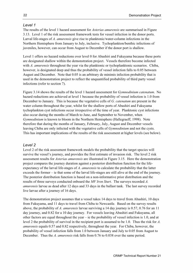
Level 1 The results of the level 1 hazard assessment for Asterias amurensis are summarised in Figure 3.13. Level 1 of the risk assessment framework tests for vessel infection in the donor ports. Larval life-stages of A. amurensis give rise to planktonic/water-column infections in the Northern Hemisphere from January to July, inclusive. Tychoplankton/benthic infections of juveniles, however, can occur from August to December if the donor port is shallow.
Level 1 offers no hazard reductions over level 0 for Abashiri and Fukuyama because these ports are designated shallow within the demonstration project. Vessels therefore become infected with A. amurensis throughout the year via the planktonic or tychoplanktonic scenarios. Chiba, however, is designated deep and thus the probability of vessel infection falls to 0.05 between August and December. Note that 0.05 is an arbitrary de minimis infection probability that is used in the demonstration project to reflect the unquantified probability of third party vessel infections (refer to section 7).
Figure 3.14 shows the results of the level 1 hazard assessment for Gymnodinium catenatum. No hazard reductions are achieved at level 1 because the probability of vessel infection is 1.0 from December to January. This is because the vegetative cells of G. catenatum are present in the water column throughout the year, whilst for the shallow ports of Abashiri and Fukuyama tychoplankton cyst infections occur irrespective of the time of year. Planktonic cyst infections also occur during the months of March to June, and September to November, when Gymnodinium is known to bloom in the Northern Hemisphere (Hallegraeff, 1998). Note therefore that during the months of January, February, July, August and December vessels leaving Chiba are only infected with the vegetative cells of Gymnodinium and not the cysts. This has important implications of the results of the risk assessment at higher levels (see below).
Level 2 Level 2 of the risk assessment framework models the probability that the target species will survive the vessel’s journey, and provides the first estimate of invasion risk. The level 2 risk assessment results for Asterias amurensis are illustrated in Figure 3.15. Here the demonstration project compares the journey duration against a posterior distribution function for the life-expectancy of the larval life-stages of A. amurensis to calculate the probability that the latter exceeds the former – ie that some of the larval life-stages are still alive at the end of the journey. The posterior distribution function is based on a non-informative prior distribution and the results of three surveys conducted onboard the MV Iron Sturt. The surveys recorded A. amurensis larvae as dead after 12 days and 33 days in the ballast tank. The last survey recorded live larvae after a journey of 16 days.
The demonstration project assumes that a vessel takes 14 days to travel from Abashiri, 10 days from Fukuyama, and 11 days to travel from Chiba to Newcastle. Based on the survey results above, the probability of A. amurensis larvae surviving a 14 day journey is 0.57, 0.76 for an 11 day journey, and 0.82 for a 10 day journey. For vessels leaving Abashiri and Fukuyama, all other factors are equal throughout the year – ie the probability of vessel infection is 1.0, and at level 2 the probability of survival in the recipient port is assumed to be 1.0. Thus the risk for A. amurensis equals 0.57 and 0.82 respectively, throughout the year. For Chiba, however, the probability of vessel infection falls from 1.0 between January and July to 0.05 from August to December. Thus the A. amurensis risk falls from 0.76 to 0.038 over the same period.

Demonstration Project
CRIMP Technical Report Number 21
23
Figure 3.13 Level 1 hazard assessment for Asterias amurensis
Figure 3.14 Level 1 hazard assessment for Gymnodinium catenatum
0
0.5
1
1.5
2
2.5
3
3.5
4
4.5
5
Jan Feb Mar Apr May Jun Jul Aug Sep Oct Nov Dec
Haz
ard
ratin
g
Abashiri Chiba Fukuyama
0
0.5
1
1.5
2
2.5
3
3.5
4
4.5
5
Jan Feb Mar Apr May Jun Jul Aug Sep Oct Nov Dec
Haz
ard
ratin
g
Abashiri Chiba Fukuyama

Demonstration Project
CRIMP Technical Report Number 21
24
Figure 3.15 Level 2 risk assessment for Asterias amurensis
Figure 3.16 Level 2 risk assessment for Gymnodinium catenatum
0
0.1
0.2
0.3
0.4
0.5
0.6
0.7
0.8
0.9
1
Jan Feb Mar Apr May Jun Jul Aug Sep Oct Nov Dec
Ris
k
Abashiri Chiba Fukuyama
0
0.1
0.2
0.3
0.4
0.5
0.6
0.7
0.8
0.9
1
Jan Feb Mar Apr May Jun Jul Aug Sep Oct Nov Dec
Ris
k
Abashiri Chiba Fukuyama

Demonstration Project
CRIMP Technical Report Number 21
25
Figure 3.16 summarises the results of the level 2 risk assessment for Gymnodinium catenatum. A journey survival model has not yet been developed for G. catenatum cysts or vegetative cells, and thus the demonstration project simply assumes that the probability of survival is 1.0. The results of the level 2 assessment therefore reflect the probability of donor port infection, and vessel infection. Since Fukuyama is infected with G. catenatum, and vessel infections occur throughout the year, the risk is 1.0 throughout the year. For vessels leaving Chiba and Abashiri, however, the risk is 0.05. This simply reflects the probability allocated to the infection status of the donor port. Note that this probability is a subjective choice that is carried through to all other levels of the risk assessment framework. A management agency may wish to adjust this value.
Level 3 The level 3 risk assessment results for Asterias amurensis are shown in Figure 3.17, and for Gymnodinium catenatum in Figure 3.18. At level 3 the risk assessment framework calculates the probability that the life-stages present in the vessel at the end of the journey will survive in the recipient port. The probability of survival is calculated relative to the temperature and salinity tolerances of the life-stages concerned, and the temperature and salinity maxima of the recipient port. In this instance the environmental data available for Newcastle is relatively poor, and thus uncertainty regarding temperature and salinity extremes in the port is described using a sample distribution function, as opposed to a kernel density estimate or extreme-value distribution (see section 6). Furthermore the port environment database does not currently hold any environmental data for Newcastle in January. The risk assessment framework therefore assumes that the probability of survival in the recipient port during this month is 1.0 for each life-stage concerned.
The results of the level 3 risk assessment for A. amurensis clearly demonstrate a decrease in risk during the Southern Hemisphere summer. As water temperatures in Newcastle increase through the summer, the probability of survival of A. amurensis larvae decreases. The actual life-stages present in the ballast tank at the end of the journey depend on those life-stages that infected the vessel in the donor port, and the life-stage duration. For example the egg/gastrula stage of A. amurensis lasts for about 3 days and will not therefore be present in a vessel whose journey is longer than this.
The results of the level 3 assessment for G. catenatum show no risk reduction for vessel leaving Abashiri and Fukuyama. This is because these ports are shallow and these vessels are infected with vegetative cells and cysts. The cysts are extremely tolerant and quite capable of surviving in Newcastle throughout the year. However, the results show a small risk reduction for vessels leaving Chiba in January, February, July, August and December. This is because during these months vessels are only infected with vegetative cells and there is a slight probability that the temperature and/or salinity in Newcastle during these months will exceed the cell’s tolerances. Note that in reality is very unlikely that the vegetative cells of G. catenatum would survive for 11 days in a ballast tank, but without a journey survival model, this is assumed to be the case for levels 2 and 3 of the demonstration project.

Demonstration Project
CRIMP Technical Report Number 21
26
Figure 3.17 Level 3 risk assessment for Asterias amurensis
Figure 3.18 Level 3 risk assessment for Gymnodinium catenatum
0
0.1
0.2
0.3
0.4
0.5
0.6
0.7
0.8
0.9
1
Jan Feb Mar Apr May Jun Jul Aug Sep Oct Nov Dec
Ris
k
Abashiri Chiba Fukuyama
0
0.1
0.2
0.3
0.4
0.5
0.6
0.7
0.8
0.9
1
Jan Feb Mar Apr May Jun Jul Aug Sep Oct Nov Dec
Ris
k
Abashiri Chiba Fukuyama

Data Collection – Module 0
CRIMP Technical Report Number 21
27
4 DATA COLLECTION – MODULE 0
4.1 Vessel-visit data The risk assessment will use information held in databases, which are periodically updated, and information that must be collected on a vessel-visit basis. The latter is collected whenever a vessel signifies its intention to enter (and deballast) in an Australian port. In the demonstration project, Module 0 asks the analyst to supply this information, namely:
• date of entry (deballast) into the recipient port;
• name of port and berth at which deballasting is to take place;
• vessel name and IMO number; and,
• details of the ballast-on-board (BOB) the vessel.
Theoretically a vessel could supply all of this information as soon as it departs the last port of call. This would allow the ballast-water risk to be calculated before the vessel arrives at the recipient port. In practise, however, there are a number of factors that might complicate this process.
The vessel’s expected arrival date will be influenced by weather and any mechanical problems encountered during the journey. Vessels may also be delayed at the recipient port because of congestion at the berth, problems with the loader, industrial action, etc. These factors could influence the risk assessment because the age of the ballast water, and the environmental conditions at the recipient port, may change significantly whilst the vessel is delayed.
On arrival at a port, a vessel in ballast will usually aim to de-ballast as safely and as quickly as possible, and avoid any delay to cargo loading. If the ballast pump can discharge ballast at a rate equal to or greater than the cargo loading rate, then the vessel may de-ballasting whilst alongside the berth. It is common, however, for vessels to start deballasting in sheltered waters outside the harbour limits. De-ballasting may then continue as the vessel proceeds to the berth (AQIS, 1993). Module 0 must therefore be capable of accurately recording where the vessel deballasts, but this may not be known prior to the vessel’s actual arrival.
Figure 4.1 show the forms used by the demonstration project to collect information on the arrival date, recipient port and vessel name. The demonstration project currently assumes that all ballast water will be discharged at the berth. In reality, however, the AQIS should allow for deballast regions outside the harbour limits and on approach to any of the berths in the port. Each of these regions could be quickly identified for a port on a one-off basis.
Figure 4.2 shows the ballast reporting form written for the demonstration project. The ballast reporting form is displayed after the vessel name and IMO number have been verified. The key elements of this form are:
• ballast details are collected on a tank by tank basis – a separate form is constructed for each tank with an explicit reference to the tank in question, eg MV Iron Sturt: Fore Peak Tank (1 of 20). The name and number of the vessel’s ballast tanks are accessed via the ship data-base (Figure 4.3);

Data Collection – Module 0
CRIMP Technical Report Number 21
28
• the form allows for multiple ballast sources within any single tank – multiple sources, times or ballasting methods can be recorded for one or more donor ports; and,
• the status of each tank must be confirmed – the “NOBOB” button (No Ballast On Board) reduces the processing time and allows the risks associated with residual ballast to be investigated.
Ideally the vessel will supply ballast-on-board (BOB) information to AQIS in an electronic format. Alternatively the vessel could fax this information using a form such as Figure 4.2. The first approach is more efficient, however, because it reduces the man-hours needed to implement the risk assessment and reduces the risk of recording errors, for example where the details recorded on the form are illegible.
All of the information collected by Module 0 is archived within the risk assessment framework. This allows audits to be conducted on any particular vessel or assessment (for enforcement or verification purposes), and also provides a means to assess the risks associated with residual ballast.
Residual ballast refers to the water that cannot be pumped out of a ballast tank because the pump line ends at some finite distance from the bottom of the tank (usually 3–4 cms). The average amount of residual ballast on board a vessel varies from about 18,000 gallons for bulk carriers to about 38,000 gallons for container ships (Carlton et al, 1995). Vessels fitted with ballast stripping systems, however, may contain less than this. The volume of residual ballast in a vessel is generally insignificant to a mariner, but is enough to support a wide variety of living organisms.
By archiving the BOB and NOBOB information supplied by vessels, it is possible to trace the source and age of the residual ballast, thereby allowing some form of risk assessment to be conducted. Within the practical constraints of a ballast reporting form, however, this will not be possible for vessels which exchange ballast water with nations who do not have an equivalent ballast reporting mechanism. It will be difficult therefore to quantify the risks associated with residual ballast until such time as equivalent reporting mechanisms are adopted internationally.
The risks associated with residual sediment are similarly difficult to quantify. The vessel-infection analysis (section 7) will indicate which vessels are likely to have taken sediment on board with their ballast. The full sediment history of the vessel, however, may not be available because of ballast reporting restraints. Sediment is rarely removed from ballast tanks – from the ship-owners perspective it is expensive and non-productive. The amount of sediment onboard a vessel, however, may be correlated with the age of the vessel, or date of last dry dock/survey.
4.2 Information held in databases The other data needs of the risk assessment are stored in databases that are updated periodically. These databases store information on vessels, ports and the target species. A detailed discussion of the data needs at each level of assessment is provided in Hayes et al (1998). The databases constructed for the demonstration project are discussed in section 3.1.

Data Collection – Module 0
CRIMP Technical Report Number 21
29
Figure 4.1 Assessment date, recipient port and vessel name forms
Figure 4.2 Ballast reporting form

Data Collection – Module 0
CRIMP Technical Report Number 21
30
Figure 4.3 Module 0 – data collection
Enter assessment date(expected entry into
recipient port)
Enter recipient port,berth and intendeddeballast locations
Enter vessel name andIMO number
Vessel Data Base
Construct ballast reportform
Enter ballast details
Verify

Data Collection – Module 0
CRIMP Technical Report Number 21
31
The Department of Primary Industries and Energy (1988) notes that the structure of all quarantine operations is fundamentally dependent on a well managed information system such as a series of technical databases. This applies equally to ballast-water risk assessment, which itself is a quarantine operation. It is not within the scope of this document to discuss the construction and management of the databases needed to support the risk assessment. There are, however, a number of points worth emphasising:
• much of the vessel data need only be collected once, for example when a vessel enters an Australian port for the first time. This information need only be updated if the vessel undergoes a major re-fit or repair;
• some vessel data, however, must be updated periodically, for example, the date of last dry dock;
• some of the port data need only be collected once, and updated only if substantial modifications are made to the port infrastructure, for example the construction of a new berth or dredging of a new channel;
• some of the port environment data should be updated on a regular basis. For example the temperature and salinity characteristics of a port should be updated on an annual basis;
• for some ports it may be possible to utilise real time environmental data. The National Oceanographic and Atmospheric Administration (NOAA) agency, for example, provides real time environmental data on the internet (http://www1.pactide.noaa.gov/ports.htm) for a number of US ports, including San Francisco Bay, Chesapeake Bay, New York/New Jersey and Houston/Galveston; and,
• the infection status of ports, with respect to target pests, should be updated on a regular basis, at least every five years for intensive surveys, but preferably on an annual basis using monitoring activities.
This last item is important because the infection status of donor ports underlies all the subsequent components of the risk assessment.

.

Port Infection Status - Module I
CRIMP Technical Report Number 21
33
5 PORT INFECTION STATUS – MODULE I
The objective of Module I is to determine whether target-species are present or absent in the recipient and donor ports(s) – ie to determine whether these ports are ‘infected’ with any of the target-species.
5.1 Background issues With a species-specific risk assessment, vessels that draw ballast water from ports that are free of target-species will ultimately be assigned a relatively low hazard/risk status. Indeed the arguments raised against species-specific ballast-water risk assessment rest largely on this point. For example, the 1996 ICES working group on introductions and transfers of marine organisms (WGITMO) recommended that ballast-water risk assessment be based on the environmental similarity of ports because:
• many port systems are often complex, with few if any previous biological surveys, and such surveys are costly, time consuming and must be repeated periodically;
• for many, if not most, animals and plants, it is not possible to quickly determine if a species in a given port could be harmful if released into a new environment; thus,
• species-specific risk assessments can only protect for a few species, and not for the many thousands that may be resident in a donor port.
Risk assessments based on environmental similarity, however, are also flawed: like the species-specific approach they will not protect against all invasive species, but unlike the species-specific approach they leave no room for improvement upon the inevitable discovery of a new ballast-water introduction (Hayes and Hewitt, 1998). Furthermore they provide very little assistance in a domestic or regional context. All vessels that trade between ports with broadly similar environments are classified as high risk. Thus they have no reactive capability when it comes to the spread of a marine pest between such areas. Environmental match risk assessments are neither reactive to the known biological hazards within ports nor completely predictive of the unknown hazards. Nonetheless, this risk assessment uses the environmental similarity between the donor bioregion and recipient port to account for non-target species.
The WGITMO concerns remain valid, and raise a number of issues in relation to the species-specific approach, notably:
• the extent to which the predictive capability of a species-specific assessment can be improved;
• how to establish (and maintain) the pest infection status of donor and recipient ports; and,
• defining appropriate risk assessment boundaries in spatially complex ports.
The first of these issues is beyond the scope of this document, but is the subject of on-going research within CRIMP. The remainder of this chapter discusses the second item in relation to donor and recipient ports. The third item is addressed in section 6.3.

Port Infection Status - Module I
CRIMP Technical Report Number 21
34
5.2 Port surveys Biological surveys normally take one of two forms – those that simply identify the presence or absence of species and those designed to enumerate species characteristics such as abundance and diversity. The first four levels of the risk assessment framework (0 to 3 inclusive) only need to know whether a target species is present or absent in a donor port. The remaining levels of the assessment (4 and 5), however, may need estimates of the population density and distribution. Moreover, all levels of the assessment need to define the probability of presence (or absence) for each target species.
The presence of a species in a port can be determined from published accounts of its presence, from museum specimens collected in the port, or through a dedicated port survey. Four types of error can occur in this process2:
• spatial Type I error – the species is recorded as present but is in fact absent when the survey is conducted. This will occur if a species is incorrectly identified;
• temporal Type I error – the species is recorded as present but is in fact absent when the risk assessment is conducted. This will occur if the target-species becomes extinct after the survey;
• spatial Type II error – the species is not recorded, nor detected by survey, but was in fact present when the survey was conducted; and,
• temporal Type II error – the species is not recored as present in the port but is in fact present when the risk assessment is conducted.
In this context, Type I errors will cause overly conservative risk estimates. In terms of environmental protection, these errors are of less concern to the risk analyst and are not considered further here. On the other hand Type II errors are inherently more dangerous because they will lead to an underestimate of risk. The remainder of this section discusses the probability of spatial Type II errors relative to port survey techniques. Temporal Type II errors can only be avoided by regularly monitoring for target species in donor ports.
Port survey techniques To date, relatively few port surveys have been conducted to identify the presence or absence of non-indigenous species3. Furthermore those that have been completed used a variety of sampling techniques. For example, Cohen et al (1998) describe rapid survey techniques for dock-fouling organisms and adjacent plankton, zooplankton and benthic infauna, which were used at 32 stations in Puget Sound over a period of 6 days. Coles et al (1997) collected fouling organisms and benthic infauna from 15 stations in Pearl Harbour, augmented by fish observations and a six-week trapping program. Hewitt and Martin (1996) describe stratified survey protocols that have been used as the foundation of a National Port Survey Program funded by CRIMP, the various port authorities and AQIS, with the assistance of the Australian Association of Ports and Marine Authorities (AAPMA). Table 5.1 summarises the sampling techniques used in each of these studies and the habitats that were sampled.
2 In defining these errors the null hypothesis is defined as the species being absent. 3 Hutchings et al (1987) list over 100 biological surveys of estuarine and near-shore coastal areas through-out Australia, few of which target port areas or elucidate non-indigenous species.

Port Infection Status - Module I
CRIMP Technical Report Number 21
35
Table 5.1 Sampling techniques used (or advocated) in port surveys for non-indigenous species
HABITAT
SAMPLING TECHNIQUE Soft substrate
Hard substrate
Seagrass/ macroalgal
Plankton/ nekton
Beach wrack
Cores/grabs 1, 2, 3, 4 2,4
Plankton/ zooplankton net 1, 2, 4
Traps – crab/shrimp 2,3 2,3 2,3 2
Visual survey – line transect 1, 2 1, 2 1, 2
Visual survey – other 1,3 1,3,4 1,3 2,3
Quadrat scraping 2
Beam trawl/benthic sled 2,4 2,4
Poison stations 2 2 1,2 1
Beach seines 2 2 2
Sediment airlift 1
KEY: 1 = after Hutchings et al (1987)
2 = after Hewitt and Martin (1996)) 3 = after Coles et al (1997) 4 =after Cohen et al (1998)
It is evident from Table 5.1 that cores, visual surveys and plankton/zooplankton nets are the most common port survey techniques. All of the studies used corers to sample soft sediment (inter-tidal and sub-tidal). The corers, however, were all of different sizes and depths, and were used at different intensity. Simple visual surveys or line transects were used in a variety of habitats, whilst vertical and horizontal net trawls were usually employed to sample the plankton and nekton.
The surveys summarised here have adopted quite different approaches. The surveys conducted by Cohen et al (1998) were almost entirely conducted from floating docks and jetties. These sites allow easy land-based access to dock fouling organisms and adjacent benthic, planktonic and nekton habitats. Access, rather than a desire to minimise the probability of a Type II error, however, dictated the survey design. By contrast Hewitt and Martin (1996) advocate detailed stratified surveys which are carefully planned, diver intensive, and take several days to complete, depending on the size of the port. The surveys are designed to maximise the likelihood that target species will be detected by sampling all suitable habitat types within the port, at those sites most likely to have been colonised by these species. Prior information on the species life-cycle and behaviour, together with knowledge of port conditions, activities and
Port Infection Status - Module I
CRIMP Technical Report Number 21
36
shipping patterns, is used to identify suitable habitats (strata) within the port boundaries, and at other adjacent sites (eg dredge spoil disposal grounds). Ground reconnaissance, aerial photographs and/or habitat maps are then used to determine habitat (strata) boundaries and the total area (or number of sites) within the port.
If a survey detects a target species, ie Pr (port infected) = 1.0 ignoring the possibility of a Type I error, then from a risk assessment perspective, each approach is as good as the other. If the survey does not detect any of target species, however, the two approaches are very different because the results of a survey whose design is dictated by ease of access cannot be used to determine the probability of a Type II error. Proper stratification and sample survey design are needed in order to achieve this.
Probability of Type II errors In the context of a port survey, the probability of a Type II error is a function of:
• the size and distribution of suitable habitat within the port environment in relation to the survey sites;
• the sample inclusion probability associated with the survey methods; and,
• the “sightability” of the species at the time of the survey.
Hewitt and Martin (1996) list 15 port areas, in order of priority that introduced species are likely to colonise. These areas cover a variety of hard and soft habitat types. Port-specific information, such as sediment maps, bathymetric surveys, etc. will also indicate other suitable habitat within the port. It is not difficult therefore to choose survey sites within suitable habitats – indeed the survey protocols that Hewitt and Martin (1996) describe are designed to do this.
Sample-inclusion probability - the probability of actually spotting a target organism with a given survey technique - has been studied by terrestrial ecologists since the turn of the century (Gates, 1979), so there is now a well developed body of theory that can be applied to marine systems. If the target organism is sessile or relatively sedentary and non-elusive, then the sample-inclusion probability can be derived from the principles of geometric probability (De Vries, 1979). These principles underpin the theories of transect sampling developed for terrestrial organisms in land-based surveys, but are equally applicable to marine organisms if similar survey techniques are employed. Most of the survey techniques described by Hewitt and Martin (1996) are identical, or equivalent, to land-based line and strip transects, and can therefore be analysed using transect sampling methods.
The sample-inclusion probabilities of the common port survey techniques (see table 5.1), are derived in Appendix A for transect surveys in poor, or near nil, visibility; plot and strip surveys that do not require visual recognition in the field; and transect surveys in good visibility. The practical application of these results, however, is limited by their assumptions, and in the case of equations [A13] and [A14], the parametric form of the detection function h(x). The detection function is usually determined empirically because it varies with organism, observer effectiveness and environmental conditions. This is done by plotting the number of organisms sighted at various distances from the transect and then fitting a curve to these results. Clearly this is not possible if no target organisms are sighted during the actual survey. Thus the analyst must use a pre-defined detection function in order to calculate the probability of a Type II error when no target organisms are sighted. Young and Young (1998) discuss several “robust”

Port Infection Status - Module I
CRIMP Technical Report Number 21
37
detection functions that perform well in a variety of situations, but the extent to which an analyst could use a (perhaps species-specific) detection function, in situations other than that in which it was originally derived remains unclear.
Importantly, the analyst can use the principles of geometric probability to calculate the sample inclusion probability irrespective of the spatial distribution of the species concerned. In particular it is not necessary for the species to be randomly distributed in the study area. However it is essential that the transect lines, points, quadrats, etc are randomly distributed within the study area (Young and Young, 1998). In practise, however, this may be difficult to achieve because of logistical or safety constraints. For example boat and dive safety considerations usually dictate which piles at a particular berth are sampled. Thus the techniques discussed in Appendix A may not be applicable to some port surveys.
The port survey protocols described by Hewitt and Martin (1996) are intensive and the sample strategy is designed around obvious environmental gradients such as habitat and depth. Thus unless the distribution of the target population is extremely limited, as might be the case in the early stages of an invasion, there is a high probability that most species will be taken at least once (Elliot, 1983). Species/area curves demonstrate that this is indeed the case for the CRIMP port surveys. At the level of the berth the species/area curve based on three replicate pile samples (Figure 5.1) does not reach an asymptote of introduced species, indicating that the berth is undersampled. At the level of the port, however, an asymptote is reached after 5 berths (Figure 5.2) indicating that few new species are detected with additional sampling sites (berths) within the port (Hewitt, 2000).
Target organisms that are cryptic or elusive - ie have a low “sightability” - are still problematic because the behaviour of the observer as well as the observed becomes important (but difficult to quantify). Motile species, for example, are often under represented in quadrats because they are disturbed when the quadrat is placed, or when it is scraped to remove the fouling organisms present (Bohnsack, 1979; pers obs). Mark and recapture methods provide population estimates for these organisms (Young and Young, 1998), but they are not designed to estimate the sample inclusion probability. Fortunately all of the target species on the current ABWMAC target list have at least one life-stage that is sessile or relatively sedentary, with the exception of Carcinus maenas and Mnemiopsis leidyi.
Sightability is also related to the temporal distribution of species in the study area. This may present problems because the timing of a port survey is usually dictated by logistic rather than biological considerations. For example surveys are usually restricted to the hours of daylight and heavily prescribed by vessel traffic within the port. Information on the species life-cycle and behaviour will indicate how significant this is likely to be. For most sessile or relatively sedentary organisms, however, it is unlikely to have a significant impact on the probability of detection. Table 5.2 summarises the probability of Type II error for each of the CRIMP survey techniques advocated by Hewitt and Martin (1996), relative to each of the ABWMAC target species. The probabilities quoted here are subjective estimates based on the authors’ experience with the survey techniques and the life-cycle characteristics of the species concerned. The estimates are designed to be used only when the analyst cannot derive objective estimates using the techniques discussed in Appendix A. The estimates quoted in the table assume that all suitable habitats in the port have been adequately sampled in accordance with the CRIMP survey protocols. These probabilities have to be translated into numerical values for the purpose of the risk assessment framework, for example 0.05, 0.5 and 0.95 for low, medium and high.

Port Infection Status - Module I
CRIMP Technical Report Number 21
38
Figure 5.1 Species/area curves of introduced species in quadrat scrapings taken at three depths from a single berth in the port Newcastle
Figure 5.2 Species/area curves of introduced species in quadrat scrapings
(summed over replicates) taken at three depths from multiple berths in the port Newcastle
0
1
2
3
4
5
6
7
0 1 2 3
Number of samples (quadrats)
Cum
ulat
ive
intro
duce
d sp
p.
0.5m 3m 7m
0
2
4
6
8
10
12
14
0 1 2 3 4 5 6 7 8
Number of sample sites (berths)
Cum
ulat
ive
intro
duce
d sp
p.
0.5m 3m 7m
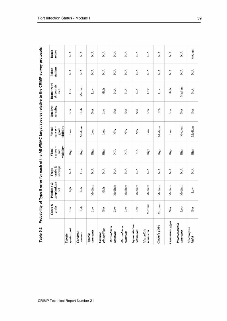
Port Infection Status - Module I
CRIMP Technical Report Number 21
39
Cor
es &
grab
sPl
ankt
on &
zoop
lank
ton
net
Trap
s –cr
abs &
shri
mps
Visu
alsu
rvey
–ba
dvi
sibili
ty
Visu
alsu
rvey
–go
odvi
sibili
ty
Qua
drat
scra
ping
Beam
traw
l&
ben
thic
sled
Poiso
nst
atio
nsBe
ach
sein
es
Sabe
llasp
alla
nzan
iLo
wH
igh
N/A
Hig
hLo
wLo
wLo
wN
/AN
/A
Carc
inus
mae
nas
Hig
hH
igh
Low
Hig
hM
ediu
mH
igh
Med
ium
N/A
N/A
Aste
rias
amur
ensis
Low
Med
ium
N/A
Hig
hLo
wN
/ALo
wN
/AN
/A
Und
aria
pinn
atifi
daN
/AH
igh
N/A
Hig
hLo
wLo
wH
igh
N/A
N/A
Alex
andr
ium
cate
nella
Low
Med
ium
N/A
N/A
N/A
N/A
N/A
N/A
N/A
Alex
andr
ium
min
utum
Low
Med
ium
N/A
N/A
N/A
N/A
N/A
N/A
N/A
Gym
nodi
nium
cate
natu
mLo
wM
ediu
mN
/AN
/AN
/AN
/AN
/AN
/AN
/A
Mus
culis
tase
nhou
siaM
ediu
mM
ediu
mN
/AH
igh
Low
Low
Low
N/A
N/A
Corb
ula
gibb
aM
ediu
mM
ediu
mN
/AH
igh
Med
ium
N/A
Low
N/A
N/A
Cras
sostr
ea g
igas
N/A
Med
ium
N/A
Hig
hLo
wLo
wH
igh
N/A
N/A
Pota
moc
orbu
laam
uren
sisLo
wM
ediu
mN
/AH
igh
Med
ium
N/A
Med
ium
N/A
N/A
Mne
mio
psis
leid
yiN
/ALo
wN
/AH
igh
Med
ium
N/A
N/A
N/A
Med
ium
Tabl
e 5.
2
Prob
abili
ty o
f Typ
e II
erro
r for
eac
h of
the
AB
WM
AC
targ
et s
peci
es re
lativ
e to
the
CR
IMP
surv
ey p
roto
cols

Port Infection Status - Module I
CRIMP Technical Report Number 21
40
5.3 Donor-port infection status If a donor port has been surveyed the probability of infection should be calculated from:
• the survey result;
• the probability of a Type II error;
• the probability that the species can actually survive in the port; and,
• the time elapsed since the survey was completed.
Figure 5.3 illustrates the assessment procedure for donor ports that have been surveyed. If the target species is detected during the survey then the probability of infection is 1.0. This remains unchanged until the responsible authority demonstrates that the species has been eradicated or has otherwise become extinct in the port.
If the target species is not detected by the survey, the probability of infection is given by
( ) ( ) error) II (TypePr ⋅= υω pp [5.1] where the probability of Type II error is calculated using the techniques discussed above, and p(υ), the probability that the species can survive in the port, is calculated using the techniques discussed in section 6.
If there are insufficient data at the level of the port to calculate p(υ), but the species can tolerate the environmental conditions of the bioregion to which the port belongs, then p(υ) is assumed to be 1.0. If the species cannot tolerate the environmental conditions of the bioregion, then p(υ) must be set to some nominally low value (eg 0.05) to reflect the analyst’s uncertainty regarding the actual port environment. Note that a bioregion’s environmental extremes, as recorded in the risk assessment database, are automatically adjusted to reflect the most extreme value recorded in any of the ports (which belong to that bioregion) for which monthly environmental data is available.
If it is impossible to calculate the probability of a Type II error, then the most conservative approach is to assume that the species is actually present in the port, the survey just did not detect it. The implication of this assumption, however, is that the risk assessment will, under certain circumstances (i.e. a lack of environmental information coupled with a poor quality survey), consider ports where target species have not been detected by survey as infected. The regulatory authority may wish to re-examine this assumption and allocate a lower probability of infection to the port.
If the port has not been surveyed it is very difficult to determine its infection status with any degree of confidence. The approach adopted by the risk assessment framework is to infer the infection status of unsurveyed international ports (outside of Australia) from that of the bioregion to which they belong. The infection status of bioregions is determined from the native and introduced distribution of the species concerned. A database detailing the bioregions of the world, adapted from the International Union for the Conservation of Nature (IUCN) (Kelleher et al, 1995), their infection status and port membership, has been developed by CRIMP. A port’s bioregion membership is easily determined by cross-reference to nation within the Fairplay ports of the world guide (Fairplay, 1998).

Port Infection Status - Module I
CRIMP Technical Report Number 21
41
Figure 5.3 Defining donor port infection status for ports which have been surveyed
CalculatePr(survival) in
the donor port?
Pr(port infected) =Pr (survival in donor port) x
Pr(Type II error)
Pr(donor port infected) = 1.0
CalculatePr(Type II error)
for survey?
Pr(port infected) = Pr(survival indonor port)
Y
N
N
Y
Y
N
Target speciesdetected?
Choose target-species
Choose donor port
Donor portsurveyed?
Y
Y Y Can the speciessurvive in thebio-region?
Pr(port infected) =Pr(Type II error)
CalculatePr(Type II error)
for survey?
Pr(port infected) = 1.0
N
Y CalculatePr(Type II error)
for survey?
Pr(port infected) = 0.05 xPr(Type II error)
Pr(port infected) = 0.05
N
N
Identify donor port bio-regionmembership
Assume species is present butundetected by survey
Assume the species is capableof surviving in the donor port
Assume that there is a smallprobability that the donor port is
infected
Port Infection Status - Module I
CRIMP Technical Report Number 21
42
The IUCN bioregions are largely based on the classification of Hayden et al (1984). This classification identifies four fundamental biomes4: open oceans, coastal margins, marginal seas and archipelagos. The coastal margins, and marginal seas/archipelagos that they contain, are further sub-divided into 40 regions on the basis of seasonal movements of air and water masses by winds and currents. Each of these regions (bioregions) refers to an area that can be justified as separate on the basis of its endemic biota or characteristic biotic association. Thus there is a clear presumption that the geophysical structure of coastal and marine environments ‘makes possible’ a particular ecological response.
At a domestic level, the risk assessment framework uses the meso-scale bioregions described in the Interim Marine and Coastal Regionalisation for Australia (IMCRA Technical Group, 1997). At the meso-scale, the coastline of Australia is sub-divided into 60 IMCRA bioregions thereby providing a much better degree of resolution for a domestic risk assessment. The IMCRA bioregions are designed to reflect coastal areas with similar biological and physical characteristics, only at a higher degree of resolution than the IUCN bioregions. As such they represent a sub-set of the first level of geographic resolution within the risk assessment framework5. Figures 5.4 and 5.6 show the IUCN bioregion distribution of Asterias amurensis and Carcinus maenas, reflecting the native and introduced distribution of these species around the world. Figures 5.5 and 5.7 show the IMCRA bioregion distribution of these species, which provides a much better resolution at the national scale
In their classification Hayden et al (1984) were unable to consider smaller scale coastal environments such as deltas, fjords and estuaries, noting that these merited a separate level of classification. Ports are commonly located in these types of environment, and thus their environmental characteristics may be very different to those of the bioregion in which they are located. This applies equally to the IMCRA bio-regions. The analyst can allow for this by calculating the probability that the species can actually survive in the port, so long as environmental data is available for the port. The probability that the port is infected can be no higher than the probability that the species can survive in the port.
Figure 5.8 illustrates the assessment procedure for donor ports that have not been surveyed. If a pest is recorded as present in a port (for example through a port survey), then the bioregion in which that port is located is construed as infected. If a bioregion is infected with a target species, the risk assessment assumes that all ports within the region are available to the target pest concerned. The probability of infection is set equal to the probability of survival, if the analyst is able to calculate the latter, otherwise the assessment conservatively assumes that the probability of infection = 1.0. If the target species has never been reported from anywhere in the bioregion, then that bioregion is assumed to be uninfected. If the target species is capable of surviving in the bioregion, and there is sufficient information from the port, then the probability of infection is set equal to the probability of survival multiplied by some nominally low value (eg 0.05). The nominally low value is a subjective probability estimate designed to reflect the analyst’s uncertainty regarding the infection status of the port. If there is insufficient information to calculate the probability of survival, or the species is unable to survive in the bioregion, then the probability of infection is simply set to the same nominally low value used above.
4 The term biome signifies an ecological formation with particular characteristics. 5 There are three levels of geographic resolution within the framework: bioregion, port and environmental sub-unit.

Port Infection Status - Module I
CRIMP Technical Report Number 21
43
Figure 5.4 International Union for the Conservation of Nature bioregion distribution of Asterias amurensis
Figure 5.5 Interim Marine and Coastal Regionalisation for Australia bioregion
distribution of Asterias amurensis

Port Infection Status - Module I
CRIMP Technical Report Number 21
44
Figure 5.6 International Union for the Conservation of Nature bioregion distribution of Carcinus maenas
Figure 5.7 Interim Marine and Coastal Regionalisation for Australia bioregion
distribution of Carcinus maenas

Port Infection Status - Module I
CRIMP Technical Report Number 21
45
Figure 5.8 Donor port infection status for ports that have not been surveyed
Choose target-species
Choose donor port
Donor portsurveyed?
Identify donor port bio-regionmembership
Is the bioregioninfected?
CalculatePr(survival) in
donor the port?
Pr(port infected) =Pr(survival in port)
Pr(port infected) = 1.0
N
Y Y
N
Can the targetspecies survive
in the bioregion?
N
CalculatePr(survival) in
donor the port?
Pr(port infected) = Pr(survival) xsmall probability to reflectuncertainty regarding theinfection status of the port
Pr(port infected) = smallprobability to reflect uncertaintyregarding the infection status of
the port
Y Y
N
Pr(port infected) = 0.05
N
Assume the species can survivein the donor port
Assume the species can survivein the donor port
Assume that there is a smallprobability that the donor port is
infected
International port?
Y
NPr(port infected) = 1.0

Port Infection Status - Module I
CRIMP Technical Report Number 21
46
5.4 Recipient-port infection status Figure 5.9 illustrates the procedure used by the demonstration project to define the infection status of recipient ports. This procedure is similar to that used for donor ports but simpler because, from a risk assessment perspective, the infection status of the recipient port is less important.
If the recipient port has not been surveyed the assessment conservatively assumes that is infected. If the recipient port has been surveyed, but the species went undetected, and is not capable of surviving in the port, then it is assumed to be uninfected. If the species can tolerate the port (based on a simple analysis of environmental extremes relative to the target species tolerances) and it is possible to calculate the probability of Type II error, the probability of infection is set to the probability of Type II error. Otherwise the assessment assumes the port is uninfected.
In the lower levels of the framework (0 and 1), the infection status of the recipient port is used within the overall hazard assessment. If a target-species is already established in the recipient port, then vessels infected with this species are considered to be less hazardous6. Thus if the recipient port has not been surveyed, the assessment conservatively assumes that it is uninfected. In the higher levels of the framework the infection status of the recipient port plays no part in the risk calculation.
5.5 Future developments Risk assessments for animal and plant imports have been conducted for many decades by various national and international agencies (Hayes, 1997). The techniques used by these agencies to determine the pest infection status of an area, and to verify this status over time, form an important precedent for managers seeking to determine the pest infection status of donor ports. For example the United Nations Food and Agricultural Organisation (FAO) recognises three types of Pest Free Areas: entire countries; an un-infested part of a country in which a limited infestation area is present; and, an un-infested part of a country situated within a generally infested area.
Techniques to establish areas as pest free, measures to maintain freedom and the checks required to verify freedom, are well established for each of these categories (Food and Agricultural Organisation, 1996, 1998a, 1998b). These provisions are implemented in Australia through AUSVETPLAN, and AQUAPLAN for terrestrial and aquatic diseases respectively. A similar approach could eventually be implemented for all marine pests, based on this model, allowing Pest Free Areas to be defined at various levels of resolution, eg IUCN bioregion, IMCRA bioregion, port, environmental sub-unit. Indeed the recent report of the National Taskforce on the Prevention and Management of Marine Pest Incursions recommends that provisions such as these be implemented nationally. This approach should also allow for ‘events-based’ reporting of incidents such as a toxic algal bloom, linked directly to the databases used by the risk assessment, for real time assessment of port infection status and vessel infection scenarios.
6 This would not be the case, however, if an active eradication program were in place at the recipient port.

Port Infection Status - Module I
CRIMP Technical Report Number 21
47
Figure 5.9 Defining recipient port infection status
Choose target pest
Recipient portsurveyed?
Can the speciestolerate the
recipient port?
Assume recipient port isuninfected
Assume recipient port isuninfected
Pr(port infected) = 1.0
Y
Y
NN
Y
N
Target speciesdetected?
Calculate theprobability ofType II error?
N
Y
Pr(port infected) = Pr (Type IIerror)
Assume recipient port isuninfected

.

Port Environments - Module II
CRIMP Technical Report Number 21
49
6 PORT ENVIRONMENTS – MODULE II
The port environment module (module II) performs three operations:
a) it measures the environmental similarity of the donor bioregions and recipient ports;
b) it tests whether target-species can tolerate the recipient port; and
c) it calculates the probability p(υ) that each target-species will survive in the recipient port.
The first operation provides a surrogate measure of ballast-water hazard that does not require species information. The second operation occurs at level 0, and is maintained at levels 1 and 2. Here module II conducts a simple tolerance test to determine whether or not a target species is likely to survive in the recipient port based on the monthly temperature and salinity extremes in the port. The third operation occurs at level 3, and is maintained at levels 4 and 5. Here module II calculates the probability that a target species will survive in the recipient port, using statistical techniques to characterise the variation in key environmental variables in the recipient port. When necessary these techniques are also accessed via Module I to calculate the probability that the species will survive in the donor port.
At level 3 the recipient port is divided into environmental sub-units. These sub-units form the geographical unit of assessment for level 3 and all subsequent levels of analysis. The berths, other deballasting areas, and sites where environmental data is collected, must be allocated to one these environmental sub-units.
6.1 Measuring environmental similarity Ballast-water risk is defined by the Ports Corporation of Queensland (PCQ) as risk = inoculation factor x environmental similarity index x risk biota factor assessment, (Hilliard and Raaymakers, 1997). The PCQ approach assumes that the probability of introduction is primarily a function of environmental similarity, for any non-native species repeatedly transferred to a new port.
The environmental similarity index (ESI) is defined as
( )( )bGMESI 1= , [6.1]
where GM is the Gower-Metric similarity coefficient, and b is the source port group number.
The GM similarity coefficient compares the k characteristics of two entities i and j, and allocates a score sijk which is zero when i and j are completely different, a positive fraction when there is some degree of similarity, and unity when i and j are identical. The overall similarity coefficient is given by
∑∑==
=n
kijk
n
kijkij sS
11/ δ , [6.2]
where δijk = 1 when character k can be compared for i and j and zero when it cannot (eg because of missing data).
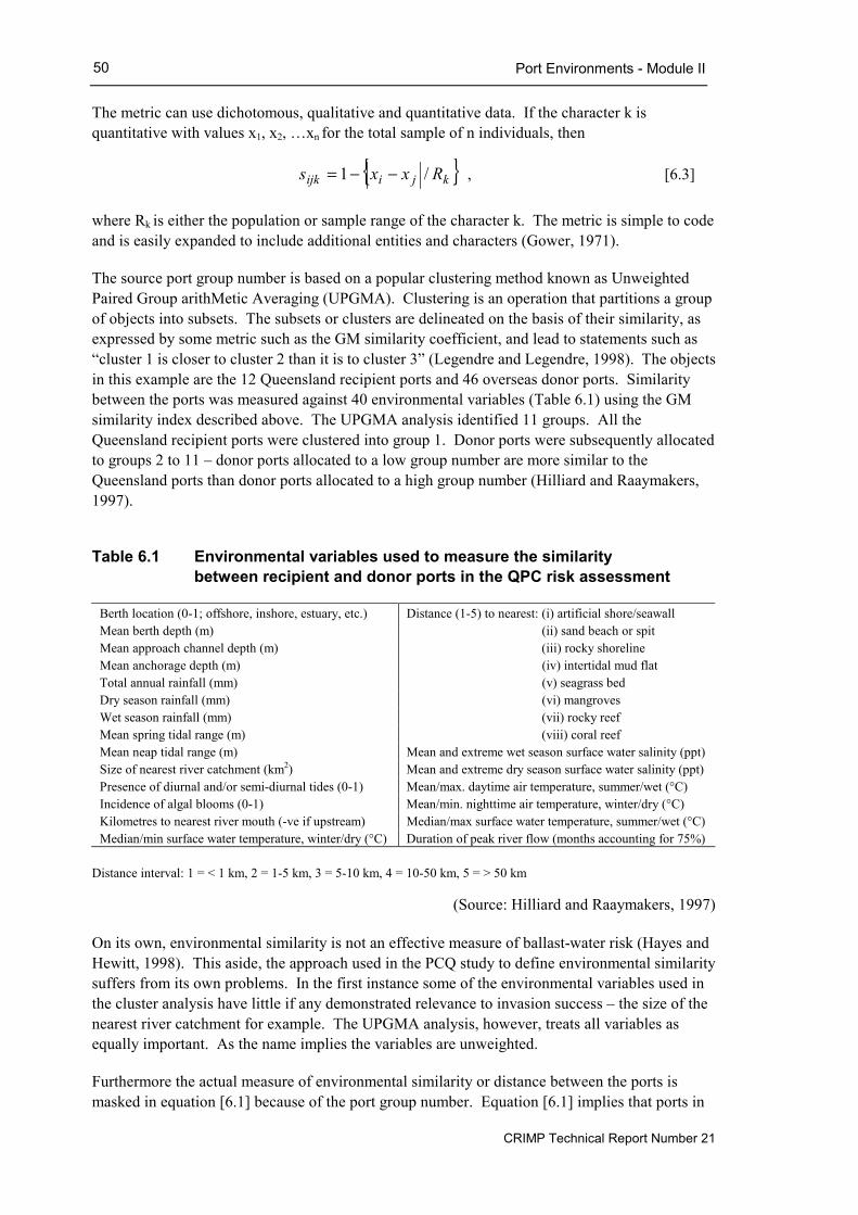
Port Environments - Module II
CRIMP Technical Report Number 21
50
The metric can use dichotomous, qualitative and quantitative data. If the character k is quantitative with values x1, x2, …xn for the total sample of n individuals, then
{ }kjiijk Rxxs /1 −−= , [6.3] where Rk is either the population or sample range of the character k. The metric is simple to code and is easily expanded to include additional entities and characters (Gower, 1971).
The source port group number is based on a popular clustering method known as Unweighted Paired Group arithMetic Averaging (UPGMA). Clustering is an operation that partitions a group of objects into subsets. The subsets or clusters are delineated on the basis of their similarity, as expressed by some metric such as the GM similarity coefficient, and lead to statements such as “cluster 1 is closer to cluster 2 than it is to cluster 3” (Legendre and Legendre, 1998). The objects in this example are the 12 Queensland recipient ports and 46 overseas donor ports. Similarity between the ports was measured against 40 environmental variables (Table 6.1) using the GM similarity index described above. The UPGMA analysis identified 11 groups. All the Queensland recipient ports were clustered into group 1. Donor ports were subsequently allocated to groups 2 to 11 – donor ports allocated to a low group number are more similar to the Queensland ports than donor ports allocated to a high group number (Hilliard and Raaymakers, 1997).
Table 6.1 Environmental variables used to measure the similarity
between recipient and donor ports in the QPC risk assessment
Berth location (0-1; offshore, inshore, estuary, etc.) Distance (1-5) to nearest: (i) artificial shore/seawall Mean berth depth (m) (ii) sand beach or spit Mean approach channel depth (m) (iii) rocky shoreline Mean anchorage depth (m) (iv) intertidal mud flat Total annual rainfall (mm) (v) seagrass bed Dry season rainfall (mm) (vi) mangroves Wet season rainfall (mm) (vii) rocky reef Mean spring tidal range (m) (viii) coral reef Mean neap tidal range (m) Mean and extreme wet season surface water salinity (ppt) Size of nearest river catchment (km2) Mean and extreme dry season surface water salinity (ppt) Presence of diurnal and/or semi-diurnal tides (0-1) Mean/max. daytime air temperature, summer/wet (°C) Incidence of algal blooms (0-1) Mean/min. nighttime air temperature, winter/dry (°C) Kilometres to nearest river mouth (-ve if upstream) Median/max surface water temperature, summer/wet (°C) Median/min surface water temperature, winter/dry (°C) Duration of peak river flow (months accounting for 75%)
Distance interval: 1 = < 1 km, 2 = 1-5 km, 3 = 5-10 km, 4 = 10-50 km, 5 = > 50 km
(Source: Hilliard and Raaymakers, 1997) On its own, environmental similarity is not an effective measure of ballast-water risk (Hayes and Hewitt, 1998). This aside, the approach used in the PCQ study to define environmental similarity suffers from its own problems. In the first instance some of the environmental variables used in the cluster analysis have little if any demonstrated relevance to invasion success – the size of the nearest river catchment for example. The UPGMA analysis, however, treats all variables as equally important. As the name implies the variables are unweighted.
Furthermore the actual measure of environmental similarity or distance between the ports is masked in equation [6.1] because of the port group number. Equation [6.1] implies that ports in

Port Environments - Module II
CRIMP Technical Report Number 21
51
group 11 are five and half times less similar, and therefore less risky, than those in group 2. This is not an objective measure, however, because the number of clusters, or port groups, is arbitrarily determined by the level of similarity that the analyst chooses when distinguishing the groups. A lower level of environmental similarity would have identified say 5 or 6 port groups resulting in a very different measure of risk.
The CRIMP risk assessment framework adopts a simpler and more conservatibve approach that avoids these problems. Here environmental similarity is measured by the GM similarity coefficient based on the monthly temperature and salinity extremes in the donor bioprovince and recipient ports, where bioprovince is defined as the broad biogeographic provincial delineations described as representing large changeovers in species. These bioprovinces thus represent surrogates for the environmental tolerances of a majority of species within the province. In practical application, bioprovinces are identified as suites of contigous bioregions. Monthly temperature and salinity extremes, for each port and their bioprovinces, are held in the port-environment database. Module II calculates the GM similarity coefficient using a weighted average of the temperature extremes for the assessment month, and the month immediately before or after this month, as follows:
( ) ( )( )
( ) ( )( )
>−+
≤−+
15date ifmonthnext max. tempq1month thismax. tempq
15 date ifmonthlast max. tempq1month thismax. tempq TWmax
where TWmax is the weighted maximum temperature and
>
−+
≤
+
=
15date if31
date315.0
15edat fi31
date5.0
q
The same algorithm is used to calculate the weighted minimum temperature, and weighted salinity extremes. The GM similarity score is used as a direct measure of environmental similarity in levels 0 and 1.
6.2 Tolerance test Level 0 conducts a simple tolerance test for each target species. This is based on the most extreme temperature and salinity tolerances taken across all life-stages, and the weighted temperature and salinity of the recipient port, as calculated above. Equivalent data for the bioregion are used if temperature and salinity data for the recipient port are unavailable.
The tolerance test is scored 1 if the temperature or salinity tolerance of the species overlaps with the expected temperature or salinity range in the donor port, and 0 otherwise. These scores are then used in the hazard algorithm of level 0 and level 1. Note that the first two levels of the framework make no judgement regarding where in the recipient port the target pest will be discharged or ultimately end up. If environmental sub-units have been defined for the recipient port, and temperature and salinity data are available for each of these units, then the most conservative (ie extreme) temperature and salinity limits should be employed in the tolerance test described above.

Port Environments - Module II
CRIMP Technical Report Number 21
52
6.3 Probability of survival The probability p(υ) that a non-native organism will survive in a recipient port is a function of:
1. the organism’s tolerance to environmental variables such as temperature and salinity; and,
2. the environmental characteristics of the recipient port.
Organism tolerances The tolerance of an organism to any environmental variable is a complex function of the magnitude of the variable, the duration of exposure, the proportion of organisms that elicit an effect and the magnitude of this effect (Suter, 1993). This function is often further complicated by various recovery and adaptation dynamics. Drake (1994), for example, notes that the physical environment (salinity, temperature, substrate, etc.) is the first filter that invading organisms meet, but warns that this is not just a physiological tolerance test. Plastic behaviour and phenotypic responses may permit invaders to survive in environments from which they would ‘normally’ have been excluded.
Risk analysts usually simplify this problem by ‘collapsing’ it along one or more dimensions. For example, by stipulating a survival endpoint, the risk assessment framework collapses the species response along the axis of effect magnitude. In other words the magnitude of effect is only expressed in terms of mortality, as opposed to reduced growth or fecundity, etc. The probability of survival thus becomes a function of the magnitude of the variable, the duration of exposure and the proportion of individuals that die. There are three ways to calculate this probability:
• calculate the stress accumulation over a finite period;
• compare published tolerance limits or dose-mortality curves against the appropriate statistical distribution function; or,
• calculate the return period of a pre-specified limit and compare this to the time needed to complete the life-stage.
To use the first approach, the analyst must fit a curve to the daily variation of the parameter in question. For temperature, the daily stress accumulation (measured in degree-days) equals the area under the curve outside the normal development thresholds of the life-stage. The analyst can calculate the probability of survival by summing the number of degree-days outside the development threshold, over the period required by the species to complete each life-stage. Furthermore, the analyst can distinguish between ‘sensitive’ and ‘hardy’ species by varying the rate at which stress accumulates and therefore the degree-days (outside the development threshold) needed to kill the life-stage.
This approach is used by CLIMEX to predict the potential geographic distribution of terrestrial plant and insect pests (Skarratt et al, 1995). It can be applied to terrestrial systems because the area under a sine curve, the amplitude of which has been adjusted to the daily maximum and minimum temperature, is a good approximation of the area under the temperature curve (see Baskerville and Emin, 1969). In marine systems current speeds and pressure changes often fit a sinusoidal model because they are predominantly driven by the tide, which is inherently regular. Temperature and salinity fluctuations, however, are much less predictable because they are driven by a variety of factors, particularly meteorological events (see for example DeVries et al, 1994). This first approach is therefore unlikely to be suitable in a marine context.

Port Environments - Module II
CRIMP Technical Report Number 21
53
In the second approach the analyst must choose a tolerance limit, such as upper lethal temperature limit, or derive a dose-mortality curve, and compare this to the appropriate statistical distribution function for the port (as discussed below). The simplest way to do this is to use published information on the tolerances of the species concerned, see for example AMBS (1997), Jansson (1994) or Pechenik (1987). Alternatively the analyst can describe a species’ tolerance through life-stage specific dose-mortality curves. The extent to which the tolerance or dose-mortality curves ‘overlaps’ with the statistical distribution function of the environmental parameter in question, provides an estimate of the probability of survival (Figure 6.1).
This approach was first applied to the geographic distribution and abundance of terrestrial populations (Andrewartha and Birch, 1954), and is similar to that used in ecotoxicological risk assessments to determine the effects of chemical contaminants (see for example Schobben and Scholten, 1993). Indeed the approach would be identical if survival probability were calculated with respect to the toxic effects of pollutants in the recipient port. In practice, however, this approach is complicated by a number of issues, notably:
• the duration of exposure;
• diet;
• pre-conditioning and acclimatisation;
• cyclic conditions and the stress rate of change; and,
• synergistic and antagonistic interactions between stressors.
At a given level of stress, mortality increases as the duration of exposure increases so that the effects of any particular stress will depend the exposure period – eg the duration of the experiment. Put another way, the time required for fatal exposure increases, as the stress becomes less extreme in relation to the species favoured range (Andrewartha and Birch, 1954). It is not immediately obvious, however, which exposure period is the most appropriate when plotting a dose-mortality curve, or what exposure period was used when a tolerance limit is published. To use published limits the analyst must check that the mortality proportion is high (at least 95%), and that the exposure period is a) less than the life-span of the life-stage concerned; and b) less than the expected residence in the recipient port. The analyst should use the same guidelines when specifying the exposure period of a dose-mortality experiment.
Food and diet history also influence an organisms tolerance to stress (Pechenik, 1987). This is an important issue for ballast-water risk assessment because the organisms diet history will be intimately linked to the duration of the voyage, ie how long it has been in the ballast tank. The analyst should be aware that organisms are often deprived of food during dose-mortality experiments to avoid the confounding influence of diet. This may lower the organism’s tolerance during the experiment.
The temperature and salinity tolerances of early larval life-stages of some species are also known to vary with the salinity and temperature experienced by the adults during gametogenesis and spawning. Similarly larvae of some species are able to acclimatise to adverse temperature and salinity regimes.

Port Environments - Module II
CRIMP Technical Report Number 21
54
Figure 6.1 Calculating the probability of survival
a b
Sample% mortality
Temperature
100
a b 50th percentile
95th percentile
For a given exposure, the % mortality varies with themagnitude of the stressor (and vice versa) - in thisexample temperature is used. The analyst mustestablish upper and lower temperature limits thatensure, for example, 100% mortality within a specifiedtime period for each life-stage of the speciesconcerned.
Variation around the LT100 is likely tooccur because of measurement error,
inter-specific variation, diet,acclimatisation and the effects of other
confounding variables
Histogram (with kernel density estimate) ofdaily minimum temperature at location x inport y for a given month
Sea temperature (0C)
95 th percentile of the LT100
A probability distribution expresses the natural variationin temperature at the recipient port. The extent to whicha specified quantile of the dose-mortality functionoverlaps with this distribution provides an estimate ofthe probability of survival. The availability of datadetermines the type of probability distribution used.Ideally a conservative approach is employed, egminimum daily temperature compared against the uppertemperature limits of the species
Area under curve givesprobability of survivalp(υ)
Probability
Port Environments - Module II
CRIMP Technical Report Number 21
55
Survival under conditions of cycling temperature can also be different to that observed experimentally under constant conditions at either end of the extreme cycle. Similarly mortality is often reduced when for example salinity is applied gradually as opposed to instances it changes abruptly. Organisms discharged from a ballast-tank are likely to be subject to an abrupt change in environmental conditions, which helps maintain a conservative stance on this issue. The issue of cyclical stress, however, is more problematic. To address this issue the analyst must examine the exposure period relative to the sampling frequency of the environmental data. Uncertainty regarding the intervening values of a parameter increases as the sampling frequency decreases. With high-frequency samples the analyst is able to check whether a tolerance limit is continually exceeded for the whole duration of the exposure period. With low frequency sampling, however, this cannot be assured, thereby compromising the accuracy of the survival probability
A synergistic interaction between stressors is another important complicating factor. A species response to a parameter such as temperature may be conditional upon the value of one or more other parameters. Sutton and Bruce (1996), for example, reported a weak dependence on temperature when investigating the effect of salinity on the development of Asterias amurensis larvae. If the mortality response of a life-stage is conditional, then it should properly be described by a multi-variate probability distribution or dose-mortality ‘surface’ in three or more dimensions. In practice, however, the mortality response is only likely to be conditional away from the limits of the species’ preferred range. Under relatively extreme conditions, causing mortality under a short exposure, the influence of other variables is likely to be small or negligible.
The third and final approach uses the EV distribution function G(x) of a parameter, to calculate the probability that the lethal limits of the life-stage will be met or exceeded over any specified period. The distribution function G(x) describes the probability of an extreme event x occurring during the sample interval from which the extreme values were originally taken - for example the daily or monthly temperature maximum. The inverse of G(x) therefore measures the expected number of intervals between successive occurrences of the event x – commonly referred to as the return time τ(x). Thus for any upper lethal-limit xul
( ) ( )ulul xG1
1x−
=τ
is the expected median number of time intervals needed to record a value > xul. A similar approach can be adopted for a lower lethal-limit xll where
( ) ( )llll xG
1x =τ
is the expected median number of time intervals needed to record a value < xll (Gaines and Denny, 1993). In both instances, the probability of survival during any period t is then given by
( ) ( )t
d.xp lτ
=υ , [6.4]
where d is the sample interval, in the same units as t. By setting t in equation [6.4] equal to the life-span of the life-stage concerned, the analyst is able to measure of the probability of survival without having to choose some arbitrary analysis period for the assessment endpoint (eg survival over a 24 hour period). The issues related to the tolerance limits of species (discussed above), however, still apply. The analyst should therefore use tolerance limits based on an exposure

Port Environments - Module II
CRIMP Technical Report Number 21
56
period that is a) less than the life-span of the life-stage concerned; and b) less than the sample interval from which the extreme values were originally taken.
In summary the stress tolerance of any given life-stage of any given species, is conditional on a whole host of factors. Indeed some authors suggest that, for this reason, laboratory data on survival under different regimes of temperature and salinity etc., may have little predictive value in the field (Pechenik, 1987). Despite this it seems reasonable to suggest that carefully researched tolerance limits, that are relatively extreme, are useful for ecological risk assessment. It is important, however, that the analyst is aware of the issues discussed above and therefore wary of single-value tolerance limits. Ultimately the analyst can allow for the effect of confounding variables by specifying mortality in probabilistic terms (Figure 6.1).
Environmental characteristics Environmental parameters are inherently variable. Probability statements therefore best describe the values that these parameters take. These probability statements are based on two sources of information – models of the environmental system in question, and observations of the parameters themselves (Ott, 1995). Environmental systems, however, are usually complex and difficult to model. Thus it is generally easier to observe the parameters of the system, and characterise its behaviour empirically, rather than attempt to model it.
Probability statements based on these observations will be accurate so long as the observations are representative of the system. To be representative there must be enough observations in space and time to record the complete range of the system’s behaviour, including any trends and seasonal variations. Probability statements based on historical observations must also assume that the system’s current or future behaviour is not radically different.
The analyst can use a number of statistical techniques to capture the variability in environmental observations (data). Each of these techniques allows the analyst to estimate the probability that a parameter will lie above or below a certain value. The quality and quantity of data, however, usually determines which of these techniques is the most appropriate on any occasion. These techniques include, in roughly increasing order of complexity:
• univariate and bivariate histograms;
• sample distribution functions;
• non-parametric kernel density estimators;
• parametric probability density functions; and,
• parametric extreme-value distributions.
Histograms are simple but effective ways of portraying data. They are also well suited to larger data sets, particularly for discrete data. Given a sample x1, x2, ... xn, an origin x0 and a bin width h, the bins of the histogram are defined as the intervals [x0 + mh, x0 + (m + 1) h) for positive and negative integers m. The histogram is then given as
( ) ( )nh
xasbin same in the xof #xf in = . [6.5]

Port Environments - Module II
CRIMP Technical Report Number 21
57
Histograms of Sydney’s sea surface temperature (SST), measured at Balmoral Beach, during June and December 1994 are plotted in Figure 6.2. The same histograms for Hobart (SST measured at mid-day just North of the Tasman Bridge) are plotted in Figure 6.3. The original data and descriptive statistics are detailed in Table 6.2.
As n becomes large, and the bin width small, a histogram approaches the density function f(x). Thus a histogram can provide an estimate of the density function, from which the analyst can draw probability estimates. The size of the data set and the choice of bin width, however, are crucial to the performance of a histogram in this regard. The choice of bin width is important because it controls the degree of ‘smoothing’, but unless the data are naturally grouped, the choice of bin width is entirely at the analyst’ discretion. This will have an important (subjective) bearing on the probability estimates drawn from a histogram, particularly for small data sets.
A sample distribution function is a much better way to represent a small data set. For any discrete or continuous random sample x1, x2, ... xn, with unknown distribution function F(x), the sample distribution function ( )xFn is the relative number of xi that are smaller or equal to x. Thus
( ) ( )∑=
≤=n
iin xxI
nxF
1
1 , [6.6]
where the indicator function ( )xxI i ≤ = 1 if xi ≤ x and 0 otherwise. A graph of the sample distribution function is constructed by arranging the sample in ascending order
( ) ( ) ( )nx........xx ≤≤ 21 and plotting
( )( )1n
ixF in += . [6.7]
The analyst, however, must subjectively determine the maximum and minimum values of the distribution function. For continuous variables these values are usually outside the observed range of the data (for example plus or minus two standard deviations). The sample distribution functions for the Hobart and Sydney SST data are shown in Figures 6.4 and 6.5 respectively. The maximum and minimum values are two standard deviations outside the observed values.
Notice that the sample distribution function ( )xFn is the frequency in n trials of the event that the variable X is less than or equal to x. As n increases ( )xFn is expected to approach the probability of the event {X ≤ x}, namely F(x) = Pr(X ≤ x). Thus, in this sense, the sample distribution function is an estimate of the underlying distribution function F(x). The analyst can draw probability estimates directly from the sample distribution function by summing the number of observations ≤ x, and dividing by n.
Sample distribution functions are popular because the analyst can use them when data is scarce. Furthermore it is easy to quantify the uncertainty surrounding the distribution function. The probability of the first order statistic (P1) is given by
),1(1 nBetaP = , [6.8] whilst the remaining order statistics (Pi; i = 2,3….n) are distributed
)P1.()]1,0(U[1P iin
1
1i −−= −+ . [6.9]

Port Environments - Module II
CRIMP Technical Report Number 21
58
Table 6.2 Sea surface temperature ( 0C ) observations for Sydney and Hobart
SYDNEY
HOBART
DATE
June 1994
December 1994
June 1994
December 1994
1
16.7
19.5
12.6
15.8
2 No data 20 12.1 15.5 3 16 18.9 12 15.5 4 16 19.5 12.1 15.8 5 No data 19 12.5 15.3 6 16 18.9 12.9 15.2 7 15.3 19 12.4 15.7 8 15 18.8 12.5 16 9 15 19.8 12.3 16.8
10 14.9 20 12.1 17 11 14.8 20 11.9 17 12 13.8 19 11.3 15.3 13 13.5 19.8 9.1 16.2 14 13 19.5 10.1 15.8 15 13.8 20.2 11 14.9 16 14.3 19.8 11.7 15.3 17 14.3 20 11.5 15.0 18 14.5 20.5 11.3 15.4 19 14.3 20.2 11 16.8 20 14 20 11.6 17.1 21 14 20.1 11.1 17.2 22 14.2 20 10.1 16.1 23 13.9 19.9 10 15.9 24 14.1 19.9 9 16.8 25 14.2 20 8.8 15.7 26 14.3 20.8 9.4 16.2 27 14.1 20 8.5 15.4 28 14.5 19 8.7 14.8 29 14.2 19.5 9.9 14.4 30 14.5 20 10.7 15.5 31
20.8 15.4
DESCRIPTIVE STATISTICS Mean Standard error Median Mode Standard deviation Range Maximum Minimum Count
14.54 0.16
14.30 14.30 0.83 3.70
13.00 16.70
28
19.75 0.10
19.90 20.00 0.54 2.00
18.80 20.80
31
11.01 0.24
11.30 12.10 1.33 4.40 8.50
12.90 30
15.83 0.13
15.70 15.80 0.74 2.80
14.40 17.20
31

Port Environments - Module II
CRIMP Technical Report Number 21
59
Figure 6.2 Histogram – Sydney SST June and December 1994
Figure 6.3 Histogram – Hobart SST June and December 1994
0
2
4
6
8
10
12
14
16
18
20
10 11 12 13 14 15 16 17 18 19 20 21 22 23 24
Sea Surface Temperature (deg C)
Freq
uenc
y
June December
0
2
4
6
8
10
12
14
16
18
6 7 8 9 10 11 12 13 14 15 16 17 18 19 20
Sea Surface Temperature (deg C)
Freq
uenc
y
June December

Port Environments - Module II
CRIMP Technical Report Number 21
60
Figure 6.4 Sample distribution functions – Sydney SST June and December 1994
Figure 6.5 Sample distribution functions – Hobart SST June and December 1994
0.0
0.1
0.2
0.3
0.4
0.5
0.6
0.7
0.8
0.9
1.0
10 12 14 16 18 20 22 24
Sea Surface Temperature (deg C)
Empi
rical
den
sity
est
imat
e F(
x
June December
0.000
0.100
0.200
0.300
0.400
0.500
0.600
0.700
0.800
0.900
1.000
6 8 10 12 14 16 18 20
Sea Surface Temperature (deg C)
Den
sity
est
imat
e
June December

Port Environments - Module II
CRIMP Technical Report Number 21
61
Appendix B describes the derivation of equation [6.8] and [6.9]. Figure 6.6 shows 100 simulations of the sample distribution function for Sydney’s sea surface temperature in December. The analyst can use these simulations to investigate some of the uncertainty surrounding the probability of survival p(υ). Figure 6.7 for example plots the frequency distribution of the probability that Sydney’s sea surface temperature will exceed 200C based on the simulations shown in Figure 6.6. Note that the mean probability estimate of the 100 simulations, 0.813, is equal to the point estimate from the original data (Figure 6.4).
An alternative way to represent data is through a kernel density estimate, defined as
( ) ∑=
−
=n
i
ihXx
Knh
xf1
1ˆ , [6.10]
where the kernel K(t) is some function which satisfies the condition
( )∫∞
∞−
= 1dttK , [6.11]
and h is the window width, smoothing parameter or bandwidth (Silverman, 1986).
The kernel estimator is essentially a series of bumps centred at each observation x1, x2…xn. The kernel function K determines the shape of the bumps, while the bandwidth h determines their width. If h is too small then the fine detail of the data masks the overall shape of the density estimate ( )xf . Conversely if h is too large the data is ‘over-smoothed’ and any detail in the density function is lost.
Placing ‘bumps’ on each observation eliminates the bin width problems encountered with histograms. Furthermore, the analyst can choose optimal versions of the kernel function K based on objective measures of discrepancy between the density estimator ( )xf and the true density f(x). In particular the mean integrated square error (MISE) defined by
( ) ( ) ( )[ ]∫ −= dxxfxfEf MISE2
, is minimised by using the Epanechnikov kernel
( )
<
−
=
otherwise0
5t5t1
543
tK
2
.
In practise, however, the kernel density function is of secondary importance because almost any reasonable kernel function gives close to optimal results (Epanechnikov, 1969). By contrast very small changes in the bandwidth can cause dramatic changes in the density estimate. Furthermore the optimal bandwidth for a kernel density cannot be calculated precisely without a priori knowledge of the distribution function f(x).

Port Environments - Module II
CRIMP Technical Report Number 21
62
Figure 6.6 Simulated sample density functions – Sydney SST December 1994
Figure 6.7 Frequency distribution for Pr (SST > 200C) in Sydney December 1994
0
10
20
30
40
50
60
70
80
90
100
0.00 0.05 0.10 0.15 0.20 0.25 0.30 0.35 0.40 0.45 0.50 0.55 0.60
Probability SST > 20 deg C
Freq
uenc
y in
100
sim
ulat
ions
0.000
0.100
0.200
0.300
0.400
0.500
0.600
0.700
0.800
0.900
1.000
17.7
18.9
19.0
19.0
19.5
19.5
19.8
19.8
19.9
20.0
20.0
20.0
20.0
20.1
20.2
20.8
21.9
Sea Surface Temperature (deg C)
Den
sity
est
imat
e F(
x)

Port Environments - Module II
CRIMP Technical Report Number 21
63
Silverman (1978) recommends plotting a test function based on the second derivative of the kernel function
( ) ( )∑=
′′=′′n
in tK
nhxf
13
1ˆ ,
for various values of the bandwidth h. The optimum bandwidth leads to a test graph that has fluctuations that are quite marked but do not obscure any systematic variation. This approach, however, is quite subjective and impossible to automate. Silverman (1986) recognises this problem and suggests an “automatic” bandwidth
51
An9.0h−
= , [6.12] where
( )34.1/range ileinterquart,min σ=A , [6.13] that provides a good fit for most unimodal and moderately bimodal probability densities. This calculation is trivial and easy to automate, although it would be wise to visually check the resulting density estimate.
From a risk assessment perspective, kernel density estimates have a number of advantages. In the first instance they can be applied to small7 and large data sets. Furthermore, provided the kernel K is everywhere non-negative and satisfies the condition [6.11] – ie is a probability density function – then it follows by definition that ( )xf will itself be a probability density. Thus, by using numerical integration, the analyst can draw probability estimates directly from a kernel density estimate. Figures 6.8 and 6.9 show the kernel density estimates, using the Epanechnikov kernel in conjunction with equation [6.12] and [6.13], for the same Hobart and Sydney SST data portrayed above. The Visual Basic code used to produce these estimates is reproduced in Appendix C.
Kernel density estimates are the most sophisticated, non-parametric, technique for displaying sample data. Beyond this, the analyst must employ parametric techniques, ie the sample data is used to estimate the parameters of a theoretical distribution. The most obvious parametric approach is to find the probability distribution that best describes or ‘fits’ the sample data. This approach assumes that the data represent a random sample drawn from the population distribution, and in practise involves finding the most likely population distribution, because it is virtually impossible to find a distribution that exactly fits the data. The first problem with a parametric approach is the large number of theoretical distributions that could describe the sample data8. Furthermore, for most distributions, testing the fit to sample data involves a computationally intensive procedure. The analyst will therefore require a software package that can perform goodness-of-fit tests quickly, for a variety of distributions, unless there is clear prior evidence to suggest a particular distribution for the parameter in question.
7 The analyst only needs 22 observations to achieve a good density estimate of a symmetrical, unimodal distribution such as the standard normal distribution (Epanechnikov, 1969). 8 Patil et al (1984a) list 62 classes of univariate and multivariate distributions for discrete data. The same authors list 108 classes of univariate distributions for continuous data (Patil et al, 1984b).

Port Environments - Module II
CRIMP Technical Report Number 21
64
Figure 6.8 Kernel density estimates – Sydney SST June and December 1994
Figure 6.9 Kernel density estimates – Hobart SST June and December 1994
0.0
0.1
0.2
0.3
0.4
0.5
0.6
0.7
0.8
0.9
1.0
10.0 12.0 14.0 16.0 18.0 20.0 22.0 24.0
Sea Surface Temperature (deg C)
Den
sity
est
imat
e
June December
0.0
0.1
0.2
0.3
0.4
0.5
0.6
0.7
0.8
0.9
1.0
6.0 8.0 10.0 12.0 14.0 16.0 18.0 20.0
Sea Surface Temperature (deg C)
Den
sity
est
imat
e
June December

Port Environments - Module II
CRIMP Technical Report Number 21
65
Figures 6.10 and 6.11 show the two most likely population distributions for Sydney and Hobart SST in June and December. The kernel density estimates are also shown for comparative purposes. These distributions were fitted to the sample data using BestFit software. BestFit uses the sample data to calculate the maximum-likelihood-estimate (MLE) of the parameters of 26 univariate distributions. There is no guarantee that the population distribution belongs to one of these – they are simply the most commonly employed statistical distributions. The software then calculates the goodness-of-fit between each of these distributions and the sample data using three tests; chi-squared, Kolmogrov-Smirnov and Anderson-Darling, and ranks each distribution according to how well it fits the data, (Palisade Corporation, 1996).
The next potential problem with the parametric approach is that the ‘best-fit’ may not necessarily be a ‘good-fit’. A poor fit often occurs in the tails of the distribution, as is clearly evident in Figure 6.11. Thus a parametric distribution may allocate finite probability estimates to values that were not actually observed, or worse, are nonsensical. The domain of the normal distribution, for example, is (−∞, ∞). This is clearly inappropriate for a variable such as sea surface temperature, although in practice it may have a negligible impact on the risk assessment. (Note that the kernel density estimator and the sample distribution function can also allocate probability to values that are not actually observed).
Cox and Hinkley (1974) suggest inter alia that a probability distribution should establish a link with any theoretical knowledge about the system in question, and should be consistent with the systems’ limiting behaviour. This type of information, however, is unlikely to be available for environmental systems without a long history of observation. Indeed, the parametric approach is generally unsuited to small data sets. This is particularly evident from Figure 6.11 – even with thirty observations the best fitting distribution is quite different from the kernel density estimate.
The tails of a parametric distribution usually over or underestimate the actual sample extremes – compare for example the tails of the parametric and kernel density estimates for SST in June in Hobart and Sydney. These extreme values, however, are often the most interesting from a risk assessment perspective. For example, Gaines and Denny (1993) note that environmental extremes are often the most ecologically significant events – particularly in relation to the survival of species. It is often better, therefore, to explicitly model the sample extremes using an extreme-value distribution.
There are three families of extreme value (EV) distributions, known as Type I, II and III, but Type I is the most common. The family of type I EV distributions, with location parameter a and shape parameter b, are given by
( )
−−−=
baxxG expexp , [6.14]
with density function
( )
−−−
−−=
bax
bax
bxg expexp.exp1
. [6.15]

Port Environments - Module II
CRIMP Technical Report Number 21
66
Figure 6.10 Probability distribution functions – Sydney SST June and December 1994
Figure 6.11 Probability distribution functions – Hobart SST June and December 1994
0.0
0.1
0.2
0.3
0.4
0.5
0.6
0.7
0.8
0.9
1.0
10.0 12.0 14.0 16.0 18.0 20.0 22.0 24.0
Sea Surface Temperature (deg C)
Prob
abilit
y de
nsity
Jun kernel T(12.9, 13.9, 16.8) Dec kernel N(19.75, 0.54)
0.0
0.1
0.2
0.3
0.4
0.5
0.6
0.7
0.8
0.9
1.0
6.0 8.0 10.0 12.0 14.0 16.0 18.0 20.0
Sea Surface Temperature (deg C)
Prob
abilit
y de
nsity
Jun kernel L(11.2, 0.94) Dec kernel I(15.8, 7659)

Port Environments - Module II
CRIMP Technical Report Number 21
67
All three families, however, can be re-stated in a single generalised EV distribution with three parameters, α, β and ε
( )β
βεαβα
1
exp
−−−= xxG . [6.16]
When applied to SST data, the ratio α/β is the maximum (or minimum) temperature achievable, ε is the most frequently occurring extreme (mode), and α represents approximately the rate of increase (decrease) of the temperature extremes with the natural logarithm of time (Jacocks and Kneile, 1974).
The term ‘extreme value’ is attached to these distributions because they can be obtained as the limiting distributions, as n approaches ∞, of the greatest value among n independent random variables, each having the same continuous distribution (Johnson et al, 1995). Although these distributions are called extreme value, it is important to note that they need not necessarily represent distributions of all kinds of extreme values, for example the extremes from small samples. They can also be used without recourse to an extreme model in the same way as any other probability distribution.
From a risk assessment perspective, EV distributions have three important advantages over other probability distributions:
• theoretically they need only be specified once because they represent the limiting distribution as the sample size increases to infinity. Thus if the environmental system does not change, then neither should the extreme value model;
• they will provide the most conservative estimate of survival probability because they describe the distribution of extreme events; and,
• a bivariate EV distribution is simply the product of the marginal EV distributions (Gumbel, 1962). Thus, the analyst does not need multivariate probability theory to simultaneously test a species’ tolerance against two or more parameters such as salinity and temperature (see below).
In practise, however, relatively large amounts of data (long time-series) are usually required to obtain an EV distribution that fits the data well. Furthermore the asymptotic theory of extreme values assumes that the data are independent and identically distributed, and therefore stationary. Long term trends (non-stationary) and autocorrelation (non-independent) within a time series are common violations of these assumptions. Trends within the data are easily removed by analysing the residuals from a regression analysis. The dependency issue, however, remains. Fortunately if the dependency between samples decreases with increasing time intervals (ie if the autocorrelation declines with increasing time lag – as in Figure 6.13), the asymptotic distribution of the extremes is the same as in the case of independent and identically distributed samples. The practical constraint is that the sampling interval should be longer than the interval between essentially independent samples (Gaines and Denny, 1993).
Figure 6.12 plots the time series of the daily maximum (and minimum) SST in the Derwent Estuary in December from 1987 to 1994. Note that data from 1988 and 1991 are missing. Regression analysis highlights a slight but significant trend: x = 15.54 + 0.007y, SP < 0.000, and the data are autocorrelated over approximately 4 or 5 days (Figure 6.13).

Port Environments - Module II
CRIMP Technical Report Number 21
68
Figure 6.12 Daily maximum and minimum SST in the Derwent, December 1987-1994
Figure 6.13 Correlogram – daily maximum SST in the Derwent, December 1987-1994
10.0
12.0
14.0
16.0
18.0
20.0
22.0
0 50 100
150
200
Date reference
Sea
surfa
ce te
mpe
ratu
re (d
egC
)
Dec max Dec min
-1.00
-0.80
-0.60
-0.40
-0.20
0.00
0.20
0.40
0.60
0.80
1.00
0 5 10 15 20 25 30 35 40 45
Time lag (days)
Auto
corre
latio
n co
effic
ient
rK

Port Environments - Module II
CRIMP Technical Report Number 21
69
Figure 6.14 compares the EVI model and the generalised EV model against the Derwent data set. The data represent the residuals of the five-day maximum temperature, with long term trend removed via regression analysis: x = 16.3 + 0.046y; SP = 0.0023. The reduced variate t is given by
( )
−=
xGt 1lnln ,
such that the inverse of the Type I distribution function is the linear function
btax += , [6.17]
whilst the inverse of the generalised function is given by
( )tx βεβα
βα −
−−= exp . [6.18]
In each case the parameters a, b, α, β and ε were estimated by optimisation – minimising the difference between the distribution functions [6.14] and [6.16] and the sample distribution function. The optimisation was performed using Evolver from Palisade Corporation because this gives better results than Excel’s Solver for non-linear functions such as [6.18]. (Note: Appendix D discusses other parameter estimation techniques and correlograms). The corresponding probability density functions are plotted on Figure 6.15 with the kernel density estimate shown for comparative purposes.
The Derwent SST data clearly deviate from the straight line described by EV I model, whilst the generalised model provides a much better fit to the data. A potential outlier, however, is evident in the data with a residual of 3.4. This corresponds to a maximum SST of 19.80C measured on December 14th 1987. This value is significantly higher than that predicted by the EV model. The model predicts an upper limit residual of 2.20 that corresponds to a temperature of 18.60C. This is clearly evident in Figure 6.15 – the upper tail of the generalised EV model falls well short of the kernel density. Indeed the EVI model provides a better fit to the upper tail of the data (but not the lower). It is not possible to be confident of the validity or otherwise of the potential outlier because of the relatively short time series available. This point does, however, underline the importance of good data and highlights how data intensive EV models can be. Jacocks and Kneile (1978) suggest 50 nominally independent samples are needed to fit an EV model. This analysis used 49 data samples taken from 6 years of data, but still remains uncertain as to the most appropriate EV model.
The amount of environmental data available to the analyst will clearly vary from port to port. The risk assessment framework accommodates this by allowing different levels of assessment depending on how much data is available. At the lower levels of analysis, the extreme temperature and salinity for each month is sufficient to characterise the port environment. Before proceeding to level 3, however, the analyst must decide whether or not there is sufficient data to allow a reasonable estimate of survival probability. There are no hard and fast rules in this context – each port is different and must be considered on a case-by-case basis.

Port Environments - Module II
CRIMP Technical Report Number 21
70
Figure 6.14 EV models – 5 day maximum SST in the Derwent, December 1987-1994
Figure 6.15 EV probability density functions - 5 day maximum SST, Derwent
-5.00
-4.00
-3.00
-2.00
-1.00
0.00
1.00
2.00
3.00
4.00
5.00
-1.50 -0.50 0.50 1.50 2.50 3.50
Reduced variate t
Res
idua
l (5
day
max
imum
)
Residual EVI General EV
0.0
0.1
0.2
0.3
0.4
0.5
0.6
0.7
0.8
0.9
1.0
-6.0
-5.3
-4.6
-3.9
-3.2
-2.5
-1.8
-1.1
-0.4 0.3
1.0
1.7
2.4
3.1
3.8
4.5
5.2
5.9
6.6
7.3
8.0
8.7
9.4
Residual 5 day maximum (deg C)
Prob
abilit
y de
nsity
kernel EVI (-0.47, 1.08) General EV (1.13, 0.34, -0.40)
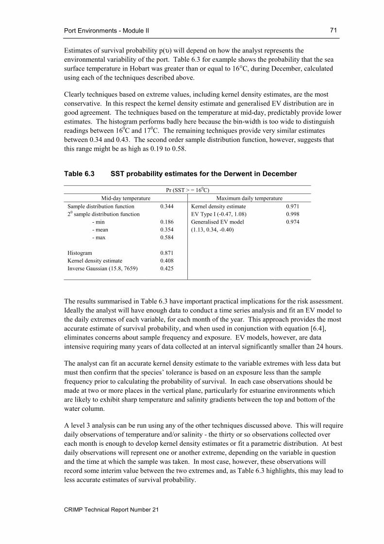
Port Environments - Module II
CRIMP Technical Report Number 21
71
Estimates of survival probability p(υ) will depend on how the analyst represents the environmental variability of the port. Table 6.3 for example shows the probability that the sea surface temperature in Hobart was greater than or equal to 16°C, during December, calculated using each of the techniques described above.
Clearly techniques based on extreme values, including kernel density estimates, are the most conservative. In this respect the kernel density estimate and generalised EV distribution are in good agreement. The techniques based on the temperature at mid-day, predictably provide lower estimates. The histogram performs badly here because the bin-width is too wide to distinguish readings between 160C and 170C. The remaining techniques provide very similar estimates between 0.34 and 0.43. The second order sample distribution function, however, suggests that this range might be as high as 0.19 to 0.58.
Table 6.3 SST probability estimates for the Derwent in December
Pr (SST > = 160C) Mid-day temperature Maximum daily temperature
Sample distribution function 20 sample distribution function - min
- mean - max
Histogram Kernel density estimate Inverse Gaussian (15.8, 7659)
0.344
0.186 0.354 0.584
0.871 0.408 0.425
Kernel density estimate EV Type I (-0.47, 1.08) Generalised EV model (1.13, 0.34, -0.40)
0.971 0.998 0.974
The results summarised in Table 6.3 have important practical implications for the risk assessment. Ideally the analyst will have enough data to conduct a time series analysis and fit an EV model to the daily extremes of each variable, for each month of the year. This approach provides the most accurate estimate of survival probability, and when used in conjunction with equation [6.4], eliminates concerns about sample frequency and exposure. EV models, however, are data intensive requiring many years of data collected at an interval significantly smaller than 24 hours.
The analyst can fit an accurate kernel density estimate to the variable extremes with less data but must then confirm that the species’ tolerance is based on an exposure less than the sample frequency prior to calculating the probability of survival. In each case observations should be made at two or more places in the vertical plane, particularly for estuarine environments which are likely to exhibit sharp temperature and salinity gradients between the top and bottom of the water column.
A level 3 analysis can be run using any of the other techniques discussed above. This will require daily observations of temperature and/or salinity - the thirty or so observations collected over each month is enough to develop kernel density estimates or fit a parametric distribution. At best daily observations will represent one or another extreme, depending on the variable in question and the time at which the sample was taken. In most case, however, these observations will record some interim value between the two extremes and, as Table 6.3 highlights, this may lead to less accurate estimates of survival probability.

Port Environments - Module II
CRIMP Technical Report Number 21
72
Weekly observations of temperature or salinity are insufficient for a level 3 analysis – the sample size per month (n = 4) is too small for any of the techniques described above. These techniques could only be employed if data over a number of years was available, aggregated over at least 4 - 5 years, to provide 20 or so observations.
For a level 0 analysis, the minimum monthly sample size is n = 2. With only two observations, however, the highest and lowest values are stipulated by default, thereby undermining the efficacy of the analysis. As the sample size increases, the range between the highest and lowest values should also increase, allowing a much more effective analysis at level 0. Again the point at which the sample size is sufficient to warrant a level 3 analysis should be decided on a case-by-case basis, but n = 30 per month, can be used as a rough guide.
Parameter considerations Having chosen how to measure the probability of survival, the analyst must choose which environmental parameters to test the species against. The parameter(s) to which the species is most sensitive is the obvious choice, but in practise this may be difficult to identify. Morgan (1995) for example suggests that at least six sources of physiological stress affect invertebrate larvae: extreme or variable temperature and salinity, low dissolved oxygen, pollution, ultraviolet radiation and poor nutrition. Generally speaking larvae are more sensitive to temperature than salinity (Pechenik, 1987) but salinity may fluctuate more extremely, particularly in estuarine environments.
The risk assessment framework advocates the use of temperature and salinity because these are important determinants of survival, and are more likely to be routinely recorded than any of the other parameters listed by Morgan (1995). The survival analysis could be extended to other parameters such as dissolved oxygen, however, if this type of data were available. Upper and lower tolerable limits are required in each case, for each life-stage of the species concerned.
The environmental extremes experienced by an organism are also dependent on its habitat and behaviour. For example, Laprise and Dodson (1993) demonstrate that in an estuarine environment sessile benthic organisms experience much greater variations in temperature and salinity than pelagic organisms. Furthermore the environmental variability experienced by pelagic animals changes according to their migratory behaviour, with tide-induced vertical migrations causing the highest short-term variability.
The risk assessment framework allows for this by defining environmental sub-units within each port (see below), and recommends that environmental data be collected for each of these. For each unit, measurements should be taken from at least two points in the water column, eg within 1m of the top and bottom, particularly for estuarine sub-units.
Multi-variate considerations At level 3 the risk assessment framework advocates calculating survival probability in relation to temperature and salinity, although it is possible to calculate the probability of survival using just one of these variables by simply assuming that the other lies within the tolerable limits of the species concerned. At levels 4 and 5 module II may also be used to extend the survival analysis to include a wider set of environmental parameters such as dissolved oxygen or pH, depending on the availability of data.

Port Environments - Module II
CRIMP Technical Report Number 21
73
Extending the survival analysis to two or more variables is simple if the variables are independent. In particular for independent variables X and Y
)Pr()Pr(),Pr( yYxXyYxX >⋅>=>> . [6.19] Thus if X represented temperature and Y salinity, the probability of survival is simply the product of the probability that these variables lie above (or below) the tolerable limits, x and y in this example, of the species concerned. If the variables concerned are correlated however, ie not independent, then this equation will lead to an inaccurate estimate of survival probability.
Salinity and temperature may be correlated within an estuarine environment because they are both influenced by cold, freshwater flows. In this instance lower temperatures are associated with lower salinity (positive correlation) such that the probability of survival is likely to be lower, for say a tropical marine species, than the estimate provided via equation [6.19]. The converse might be true, however, if two variables were negatively correlated, as might be the case for temperature and dissolved oxygen in effluent outfall of an industrial plant.
If any of the environmental parameters used in the survival analysis are dependent then their distribution function should properly be represented with a bivariate or multi-variate distribution function, and the probability of survival calculated accordingly. Kernel density estimates and parametric distribution functions can be defined for these variables, and probability estimates drawn from these using numerical integration. Mathematically this is more demanding, however, and therefore is usually accomplished using an appropriate software package.
The degree of dependence between two random variables X, Y can be measured using a variety of correlation coefficients. If two variables are independent then the correlation coefficient is 09. Pearson’s product-moment correlation coefficient, denoted r, is one of the most common methods (although most correlation coefficients give similar results with reasonable data sets).
Other useful measures of monotonic (that is always moving in a consistent direction) association, which are distribution-free, include the Spearman rank correlation coefficient, denoted rS, and Kendell’s tau correlation coefficient, denoted tτ. The latter is particularly useful as the basis for the hypothesis that the variables are uncorrelated, without having to make any assumptions about the underlying population distribution (see McPherson, 1990 for details). It is also possible to test for independence amongst three or more variables using an equivalent multi-variate technique based on the correlation matrix. This approach, however, assumes that the observations are drawn from a population with a multi-variate normal distribution, which may not always be the case (see Legendre and Legendre, 1998 for more details).
Note that the analyst does not need to test for independence if he or she is able to specify EV distribution functions for the environmental parameters concerned. This is because a bivariate EV distribution function G(x, y) is simply the product of the marginal EV distributions G(x) and G(y). The analyst can therefore treat probability estimates drawn from these distributions as independent and can therefore calculate the probability of survival as per equation [6.19].
9 Strictly speaking, however, the inverse implication is not true – ie if the correlation coefficient is 0 the variables are independent. In practise, however, the correlation coefficient is used as a measure of dependence or independence between variables.

Port Environments - Module II
CRIMP Technical Report Number 21
74
Environmental sub-units Most port-environment data is collected at discrete sampling stations. It is possible to ‘map’ some environmental variables in a continuous fashion (see for example Miller et al, 1998) but this technology is not widely available. The area which discrete data represents must (to some reasonable extent) be vertically and horizontally homogenous. The administrative boundaries of most ports, however, encompass areas that are not homogenous, and cannot therefore be represented by a single sample site. Freemantle for example has berths within the mouth of the Swan River, an estuarine environment, and in Cockburn Sound, a coastal environment. The salinity characteristics of these two areas are likely to be quite different.
The CRIMP framework accommodates this by defining environmental sub-units within each recipient port. These sub-units delineate areas within the port that are environmentally similar, and are analogous to the delineation of eco-regions based largely on climatic similarity (Bailey, 1983). Environmental sub-units may reflect natural distinctions, for example between estuarine and coastal habitats, or man-made distinctions, such as micro-habitats caused by power station outfalls. In general terms, environmental data should be collected for each environmental sub-unit in a port. This data should be collected from at least two points (top and bottom) in the water column, particularly for estuarine sub-units.
Small ports may encompass a single environmental sub-unit. Burnie for example, has an open coastal environment. A single sampling station could therefore represent the whole port. Larger ports may comprise of two or more sub-units - Newcastle for example could have five distinct sub-units (Figure 6.16):
• harbour entrance/offshore – an open, coastal environment;
• the Hunter river & Throsby Creek – a brackish/fresh riverine environment;
• the horse-shoe – an intermediate, estuarine environment;
• the steel-works channel – an artificially maintained, deep-water basin, with unrestricted circulation, that receives effluent input from the BHP steel-works; and,
• the west basin – an artificial shallow-water basin with restricted circulation.
Important commercial berths are located in three of these – the horse-shoe, steel-works channel and west basin. Vessels may also de-ballast offshore and in the harbour entrance, on approach to these berths. Newcastle may therefore need four sampling stations to properly characterise the port environment.
Maps, aerial photographs, existing data and the results of port surveys will indicate where the boundaries between environmental units lie. In many instances, the distribution of species within a port will reflect these distinctions (Hewitt, unpub data). Drawing the boundaries between sub-units, however, is ultimately a subjective process and should be done by persons who are familiar with the port. The environmental sub-units need only be defined once, unless substantial modifications are made to the port.

Port Environments - Module II
CRIMP Technical Report Number 21
75
Figure 6.16 Possible environmental sub-units within the port of Newcastle
Harbour entrance/offshore
Hunter river/Throsby creek
Horseshoe
Steelworks channel
The Basin

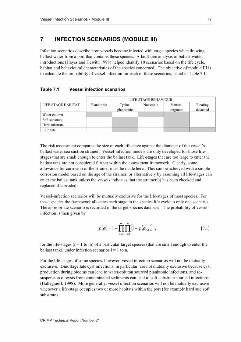
Vessel Infection Scenarios - Module III
CRIMP Technical Report Number 21
77
7 INFECTION SCENARIOS (MODULE III)
Infection scenarios describe how vessels become infected with target species when drawing ballast-water from a port that contains these species. A fault-tree analysis of ballast-water introductions (Hayes and Hewitt, 1998) helped identify 10 scenarios based on the life cycle, habitat and behavioural characteristics of the species concerned. The objective of module III is to calculate the probability of vessel infection for each of these scenarios, listed in Table 7.1.
Table 7.1 Vessel infection scenarios
LIFE-STAGE BEHAVIOUR LIFE-STAGE HABITAT Planktonic Tycho-
planktonic Nuestonic Vertical
migrator Floating detached
Water column Soft substrate Hard substrate Epiphyte
The risk assessment compares the size of each life-stage against the diameter of the vessel’s ballast water sea suction strainer. Vessel-infection models are only developed for those life-stages that are small enough to enter the ballast tank. Life-stages that are too large to enter the ballast tank are not considered further within the assessment framework. Clearly, some allowance for corrosion of the strainer must be made here. This can be achieved with a simple corrosion model based on the age of the strainer, or alternatively by assuming all life-stages can enter the ballast tank unless the vessels indicates that the strainer(s) has been checked and replaced if corroded.
Vessel-infection scenarios will be mutually exclusive for the life-stages of most species. For these species the framework allocates each stage in the species life cycle to only one scenario. The appropriate scenario is recorded in the target-species database. The probability of vessel-infection is then given by
( ) ( )[ ]∏∏= =
−−=m
r
n
iirpp
1 1,11 φφ , [7.1]
for the life-stages (r = 1 to m) of a particular target species (that are small enough to enter the ballast tank), under infection scenarios i = 1 to n.
For the life-stages of some species, however, vessel infection scenarios will not be mutually exclusive. Dinoflagellate cyst infections, in particular, are not mutually exclusive because cyst production during blooms can lead to water-column sourced planktonic infections, and re-suspension of cysts from contaminated sediments can lead to soft-substrate sourced infections (Hallegraeff, 1998). More generally, vessel infection scenarios will not be mutually exclusive whenever a life-stage occupies two or more habitats within the port (for example hard and soft substrate).

Vessel Infection Scenarios - Module III
CRIMP Technical Report Number 21
78
7.1 Water column Holoplanktonic and meroplanktonic species complete all or part of their life cycle in the water column. The target-species database records which life-stage(s) live in the water column, whilst Module III determines when these life-stages are actually available to ballasting vessels.
Planktonic Level 1 uses a simple approach to model planktonic water-column infections. The target-species database records the presence or absence of each life-stage during each month of the year – all vessels that ballast during those months when the life-stages(s) are recorded as present, are assumed to be infected, ie p(φ) = 1. The presence or absence of life-stages can be inferred from the published life-cycle characteristics, vessel-infection history or port surveys.
Asterias amurensis for example has five life-stages: egg/gastrula, bipinnaria, brachiolaria, juvenile and adult. Vessel-infection scenarios for each life-stage are mutually exclusive. The larval life-stages, egg/gastrula, bipinnaria and brachiolaria, can cause water-column sourced, planktonic infections. Like many echinoderms, the larvae spend a relatively long time in the plankton. In the Derwent estuary larvae are likely to be in the water column from July to January (Byrne et al, 1997; CSIRO unpublished data). In a level 1 analysis, vessels ballasting in Hobart during this period would be classified as infected p(φi, r) = 1.0 where i = 1 = water-column/plankton and r = 1 to 3 = the three larval life-stages.
At levels 4 and 5, the presence of a life-stage could be determined inductively on the basis of spawning/blooming cues and environmental triggers, and expected residence time. For example, Blackburn et al (1989) indicates that in southern Tasmania, Gymnodinium catenatum blooms when water temperatures range from 12-180C and salinity range from 28-34‰. Blooms are also possibly triggered by heavy rainfall events that contribute nutrients to the water column from land run-off. Furthermore at level 5, Module III is expected to model the horizontal and vertical distribution of planktonic life-stages based on the behavioural characteristics of the life-stage, the port-distribution of the species and the circulation patterns of the donor port.
Nuestonic Nuestonic organisms live at or near the air-sea interface, and may not therefore be available to vessels drawing ballast at some depth below this. At level 1 no allowance is made for the vertical distribution of planktonic organisms, and thus Module III simply treats neustonic infections as planktonic water-column infections. At higher levels of analysis, however, neustonic infections only occur if the ballast-water envelope intersects or approaches the air-sea interface.
The ballast-water envelope refers to the ‘parcel’ of water that is sucked into a vessel when ballast is pumped onboard. Hunter (1997) develops a simple model for a hydrodynamic sink that describes the shape and dimensions of this parcel, as a function of the pump rate, duration, ambient current and initial boundary conditions. The solution for the velocity field due to the combined effects of the sink (ballast inlet) and any ambient current is
( )23
2224 ZYX
XcU++
−=π
Vessel Infection Scenarios - Module III
CRIMP Technical Report Number 21
79
( )23
2224 ZYX
YV++
−=π
[7.2]
( )23
2224 ZYX
ZW++
−=π
.
X, Y and Z are non-dimensional spatial coordinates given by
zqpZ
yqpY
xqpX
21
21
21
=
=
=
, [7.3]
where (x, y, z) are the spatial coordinates (in metres), p is the ambient current rate (in ms-1) and q is the flow rate into the sink – ie the rate at which ballast is pumped on board (in m3s-1). From equation [7.3] dimensionless water velocities are defined
pwW
pvV
puU
=
=
=
, [7.4]
where (u, v, w) are the water velocity components (in ms-1). Equations [7.1] – [7.4] define the horizontal and vertical dimensions of the ballast-water envelope for any non-dimensional pumping time P given by
tqpP
21
3
= . [7.5]
In practise, however, the dimensions of the ballast envelope may also be influenced by other extrinsic factors, notably port structures, and the activity of other vessel traffic. Thus whilst the theory is relatively well developed, the data requirements preclude an analysis of the ballast envelope at the lower levels of the framework.

Vessel Infection Scenarios - Module III
CRIMP Technical Report Number 21
80
Vertical Migrator Many of the larval life-stages, of a wide variety of species, control their horizontal distribution and dispersal by navigating vertically in the water column. In estuaries, for example, the net transport of plankton depends upon their depth distribution because the net flow is landward low in the water column, and seaward at the surface. Thus estuarine larvae can control both the speed and direction of transport by regulating how long they spend at each depth (Cronin and Forward, 1982).
Vertical migration may be initiated or restricted by at least nine environmental cues, including salinity, temperature, water currents, gravity and light (Young, 1995). In some cases the larval response to these cues is complex, involving the interplay of endogenetic and exogenetic factors, and may change ontogenetically10. It is important, however, that the life-stage response can be approximated by simple “bio-rules” that describe the vertical distribution of larvae, in order to estimate whether or not the distribution overlaps with the vertical dimensions of the ballast-water envelope.
The most common patterns of vertical migration are diel and tidal. Diel migrations occur on a daily basis and can be broadly classified into one of three types (Forward, 1988) that could form the basis of a simple bio-rule:
• nocturnal – a single daily ascent starting at sunset, minimum depth reached during the night. Descent occurs at sunrise, maximum depth attained during the day;
• twilight – a rise to minimum depth occurs at sunset, followed by a descent later in the night (the ‘midnight sink’). Another ascent occurs at sunrise followed by a descent to the daytime depth; and,
• reverse – a single daily ascent starting at sunrise, minimum depth reached during the day. Descent occurs at sunset, maximum depth attained during the day.
Tidal migrations can be similarly classified according to whether ascent to minimum depth occurs on a flood or ebb tide. Vertical migration can impose a distinct day/night or flood/ebb differential on the depth distribution of many species. Vertical migrations of several hundred metres have been observed in open ocean systems (Rudyakov, 1979), but the displacement is presumably much smaller in estuarine and coastal systems. Furthermore a range of exogenous factors may influence the minimum depth attained during ascent. Thorson (1964) for example suggests that light intensity, temperature and salinity often act in unison to keep larvae away from the uppermost layers of the water column. Bruce (1998) notes that the larval life-stages of Asterias amurensis exhibit a low-kinetic response (eg cessation of swimming) to low-salinity water that keeps them out of the surface layers of the upper Derwent estuary. Similar halokinetic and thermokinetic responses are summarised by Young (1995).
It is important, however, not to confuse random movement in the absence of a stimulus, with vertical migration. For example if the behavioural repertoire of a species is limited to negative phototaxis, then by day virtually all members of a population will be driven into deeper water. By night, however, random movement will cause the population centre to shift upwards. In essence vertical migration requires at least two different behaviours – one to move organisms up, the other to direct them down (Young and Chia, 1987).
10 As the organism develops or grows.

Vessel Infection Scenarios - Module III
CRIMP Technical Report Number 21
81
For the purposes of the risk assessment framework three criteria must be met in order to model vertical migration patterns:
• the vertical migration pattern must be predictable;
• the maximum and minimum depth limits attained on descent and ascent must be defined; and,
• the population must have a reasonably discrete depth distribution.
In a shallow port environment, however, it is unlikely that any of the criteria will be met. The water column in a port is routinely disturbed by vessel traffic and propeller induced turbulence (Section 7.2). This may increase turbidity, reduce light penetration, periodically eliminate pycnoclines and physically eliminate the ‘natural’ depth profile of a population. Furthermore harbour lighting may alter the natural light/dark cycle which induces most diel migration patterns.
The vertical extent of the ballast-water envelope will typically be of the order of 2.5 metres above and below the level of the intake (Hunter, 1997). The species distribution must lie outside of this envelope for the duration of the ballast operation in order to influence the probability of infection. For this reason, and those above, vertical migration may only influence the probability of vessel infection in deep-water ports, under very specific conditions.
The effect of vertical migration on the probability of vessel infection cannot be determined without a model of the ballast envelope, as described above. Again, whilst the theory for such a model is well developed, the additional data requirements, including the salinity and temperature profile of the water column and the activity of third-party vessels, precludes such an analysis at the lower levels of the framework. At levels 1 to 3 it is only safe therefore to assume that water-column sourced species are uniformly distributed through-out the water column.
The modelling approach used in the higher levels of the framework (4 and 5) must be species-specific, and will depend on whether migration is controlled by endogenetic or exogenetic factors. Tidal migration patterns can be controlled by both endogenetic and exogenetic factors (compare for example Queiroga et al, 1997 and DeVries et al, 1994), whilst diel migration is usually controlled by exogenetic factors – predominantly light (see the review in Forward, 1988).
Migration patterns that are controlled by light or endogenetic rhythms are quite predictable, allowing for possible complications caused by artificial lights. In many instances then the first modelling criteria will be met quite easily. The remaining criteria, however, are much more problematic and in most cases will require a detailed survey of the species’ behaviour in the port environment. This type of analysis will only be cost-effective in very specific “high-risk’ situations, where substantial risk reductions cannot be achieved in the journey survival or port survival components of the framework.

Vessel Infection Scenarios - Module III
CRIMP Technical Report Number 21
82
7.2 Soft-substrate sources Soft-substrate (sediment) sourced life-stages are only available to ballasting vessels if:
1. they are passively re-suspended into the water column; or,
2. they actively migrate into water column.
Tychoplankton Life-stages that are passively re-suspended into the water column are categorised as tychoplankton and treated as particulates, with some allowance for motile behaviour where appropriate. Life-stages that periodically migrate into the water column are categorised as vertical migrators, irrespective of their habitat.
Particulates can be suspended into the water column of a port through natural events, vessel induced events or by other port-based engineering activity. In this context, the objective of Module III is to distinguish between donor ports that are ‘shallow’ – re-suspension could or is occurring, and those that are ‘deep’ – re-suspension does not occur.
At level 1 a port can be classified as ‘shallow’ or ‘deep’ on the operating experience of the harbour master or port manager. For a deep port p(φ) = 0.05 for soft-substrate tychoplankton organisms because re-suspension is not occurring and thus these organisms cannot be entrained within the ballast tank. For a shallow port, however, p(φ) is assumed to be 1. If there is any doubt, the port should be classified as ‘shallow’.
At levels 4 and 5 the environmental units of a port are classified as ‘shallow’ or ‘deep’ according to the ‘natural’ vertical concentration-profile of particulates, vessel or engineering induced re-suspension and the ballast envelope of the vessel. Thus whilst some ports may clearly fall into the category of ‘deep’, for others their status may be a function of vessel activity, tidal state and particle characteristics such as size, shape and density.
In particular, the analyst must determine at least four components of this function in order to model tychoplankton infections:
• the critical bed velocity for the particle;
• the particle’s sinking velocity;
• the natural flow characteristics of the environmental sub-unit in question; and,
• the vessel-induced flow characteristics of the sub-unit.
When water flows over a bed of loose particles there is a certain velocity at which the combined drag and lift forces on the uppermost particles are sufficient to dislodge them from their rest position. Particles will start to move when the flow exerts a sheer-stress at the bed τ0 that exceeds the critical sheer-stress τcr for the particles in question. For a flat bed, in the absence of waves, flow velocity and bed sheer-stress are related by the quadratic stress law (Dyer, 1985)
20D0 uCρ=τ , [7.6]

Vessel Infection Scenarios - Module III
CRIMP Technical Report Number 21
83
where CD is a drag coefficient, ρ is the fluid density and u0 is the near-bed flow velocity. In practise, however, is difficult to define near bed flow velocities and thus it is common to express this relationship in terms of currents measured at one metre above the bed, such that
21001000 uCρ=τ . [7.7]
The drag coefficient at this height (C100) has been determined experimentally for a variety of bed types, ie 2.2 x 10⁻³ for mud, 2.6 x 10⁻³ for unrippled sand and 4.7 x 10⁻³ for gravel. The drag coefficient is also influenced by bed-forms, rising for example to 6.1 x 10⁻³ for rippled sandy beds (see Dyer, 1985 for details).
The critical bed shear-stress τcr can be determined from van Rijn’s interpretation of the Shield’s entrainment function (van Rijn, 1993). By defining a dimensionless particle parameter d*
31
250*g)1s(dd
υ−= , [7.8]
the critical Shield’s parameter θcr can be represented as
150dfor 055.0150d20for d013.0
20d10for d04.0
10d4for d14.0
4d1for d24.0
*cr
*29.0
*cr
*10.0
*cr
*64.0
*cr
*0.1
*cr
>=θ≤<=θ
≤<=θ
≤<=θ
≤<=θ
−
−
−
The critical Shield’s parameter is related to the critical shear stress according to the equation
( ) 50crcr gd1s ρ−θ=τ . [7.9] As the bed-shear velocity reaches values defined by equations [7.6] to [7.9], particles at the surface of the bed begin to jump and roll along the bed (saltation) forming the ‘bed-load’ layer. Unless the ballast envelope extends into the bed-load, tychoplankton infections cannot occur until the particles are actually suspended into the water column. Suspension occurs when the value of the bed shear velocity becomes comparable to the particles’ fall velocity (ws) in still water. Van Rijn (1993) suggests that suspension begins to occur when
( )( )
( )( )
( ) 10dfor gd1s
w16.0
10d1for gd1s
wd16
*50
2s
cr
*50
2s
2*
cr
>−
=θ
≤<−
=θ , [7.10]
whilst a fully developed concentration profile starts to develop when
( )( ) 50
2s
cr gd1sw
−=θ . [7.11]

Vessel Infection Scenarios - Module III
CRIMP Technical Report Number 21
84
A concentration profile starts to develop when the surrounding fluid supports the particle’s weight. However, since inert particles continuously settle at a rate determined by their settling velocity (ws) relative to the surrounding fluid, a continuous or equilibrium suspension is only possible if the fluid flow provides a countermotion which raises the particles with an equal velocity (Chow, 1964). This upward countermotion is provided by turbulent exchange within the fluid – rising fluid originates from layers closer to the sediment/water interface with a higher particle concentration, whilst descending fluid originates from higher layers with a lower concentration. As a result, a surplus of upward moving particles over the downward moving particles occurs. This surplus provides the upward motion of particles that counterbalances the general settling (Figure 7.1a). The vertical concentration profile that results can be described by the Rouse equation
( )( )
−−=
*
s
a
z
u4.0w
expahzzha
cc
, [7.12]
where cz is the particle concentration at a distance z above the bed, h is the total water depth, ca is the particle concentration at a reference distance a above the bed and u* is the friction velocity at the bed given by
( )2*0 uρ=τ . [7.13]
Taking the natural logarithm simplifies the Rouse equation such that the particle concentration profile is linear. Thus for large particles in a relatively slow flow (ie large ws/u*) the upper layers of the water column are clear, whilst for small particles in a fast flow (ie small ws/u*) there will be a relatively high concentration of particles throughout the water column (Figure 7.1b). Figure 7.1c shows the vertical concentration profile for different values of the exponent in the Rouse equation.
The height of the reference layer a in the Rouse equation is usually taken to be upper edge of the bed load layer (Figure 7.1b). The reference concentration ca is defined to be equal to the average sediment concentration in the bed-load layer cb. Van Rijn (1993) provides the following equations for the height of the bed-load layer, and the average bed-load concentration
( ) ( ) 5.07.0*50 Tdd3.0a = , [7.14]
and
*0b d
Tc18.0c = , [7.15]
where c0 is the static bed concentration11 of the particles, and T is the ‘excess’ bed shear-stress parameter given by
( )cr
cr0Tτ
τ−τ= . [7.16]
11 This must be multiplied by the particle density to provide an estimate of the concentration by weight (kg/m3).

Vessel Infection Scenarios - Module III
CRIMP Technical Report Number 21
85
Figure 7.1 The concentration profile and Rouse equation
b) The vertical concentration profile is linear when plotted on logarithmicscales
loge depth
a
loge particle concentration
A
B
Ca
A = downward settling/upward diffusion = largeB = downward settling/upward diffusion = smallCa= particle concentration at reference depth a
a) The vertical concentration profile is determined by the ratio of the particles settlingvelocity (ws) and turbulent exchange between horizontal layers of different particleconcentration
Sea bed with particle concentration C0
Turbulent exchange ofmomentum andparticles betweenhorizontal layers providesurplus upwardtransport
Direction of flow
Waterdepth
(z)
Z/h
c/ca
0.2
0.4
0.6
0.8
1.0
0.2 0.4 0.6 0.8 1.0
Reference height a
Bed load occursbelow referenceheight
A: Ws/κu* = 2.5
B: Ws/κu* = 1.0
C: Ws/κu* = 0.1
A
B
C
c) Relative concentration profiles for different values of the exponent in the Rouseequation

Vessel Infection Scenarios - Module III
CRIMP Technical Report Number 21
86
A particle’s sinking velocity is principally a function of its shape and size (expressed in terms of the ratio of surface area to volume) and its density relative to that of the fluid through which it is moving. The sinking velocity of a particle can be estimated theoretically on this basis. For example Sarjeant et al (1987) derive a modified version of Stokes Law to describe the sinking velocity (ws) of dinoflagellate cysts
µ3/2 1grmws = [7.17] where r is the radius of the particle (in cm), and µ is the absolute viscosity of the fluid. m1 is the excess mass per unit area of the phragma given by
( )ερρ −= sm1 [7.18] where ρs is the density of the sporopollenin and ε is the wall thickness.
For most biological particles, however, the relationship between cell density, size, shape and sinking velocity is considerably more complex because it is influenced by numerous additional factors including cell viability and physiology, growth rate, protuberances, motile behaviour and (possibly) structural viscosity (Smayda, 1970). As a result, the settling velocity of individual organisms is usually estimated empirically either in laboratory settling chambers or by comparing changes in population density with depth in the field (although the latter is complicated by natural phenomena such as losses due to zooplankton grazing and advection). Table 7.2 provides some examples of sinking rates available in the literature for phytoplankton as compared to zooplankton and fish eggs, demonstrating the considerable variability that is often observed in these types of studies.
Table 7.2 Sinking rates12 of phytoplankton, zooplankton and fish eggs
GROUP SINKING RATE (cm s-1)
NO. OF SPECIES
REFERENCE
Phytoplankton Living Dead (intact) Dinoflagellate cysts
0 - 0.035
0.001 - 0.590 0.008 - 0.015
∼ 25 10 4
Smayda (1970) Anderson et al, (1985)
Zooplankton Amphipoda Chaetognatha Cladocera Copepoda
∼ 1.013 ∼ 0.503
∼ 0.139 - 0.185 0.042 - 0.833
1 1 2
14
Quoted in Smayda, (1970)
Faecal pellets 0.042 - 0.435 na Quoted in Smayda, (1970)
Fish eggs 0.249 - 0.463 2 Quoted in Smayda, (1970)
12 Note that these values are only good for the test conditions under which they were determined. For example Anderson et al (1985) suggest that a 100C drop in temperature would reduce the sinking rates they quote by 22%.

Vessel Infection Scenarios - Module III
CRIMP Technical Report Number 21
87
There are a number of mechanisms that can give rise to accelerated sinking rates well in excess of those quoted above including coagulation and/or formation of chains, and the attachment of phytoplankton cells to abandoned larvacean houses or ‘marine snow’, (Kiorboe et al, 1996; Sarjeant et al, 1987). Processes which increase a particle’s sinking velocity will tend to reduce the probability of tychoplankton infection, leading to conservative risk estimates if ignored.
Smith (1982) notes that under turbulent flows, the amount of algal material in suspension declines exponentially with time, but during periods of calm algae settle at an enhanced rate described by Stokes Law. Condie and Bormans (1997), however, suggest that turbulence is often suppressed in stratified regions of flow, such that settling velocity alone controls transport in this region. Again, these processes will tend to decrease the probability of tychoplankton infection.
There may also be a number of other factors that influence the vertical concentration profile of pest organisms such as deposited dinoflagellate cysts. For example Sarjeant et al (1987) report that dinoflagellate cysts may concentrate in the unconsolidated or flocculative upper layer of the bottom sediment, and would therefore be readily resuspended. However, Anderson et al (1985) note that cysts usually become well buried in the sediments by biological activity (thereby decreasing the particle concentration in the bed-load cb) and may also adhere to other particles in the sediment due to mucilage production and entanglement (thereby increasing the critical bed shear-stress τcr). For the purposes of the risk assessment it is safer to assume that all sediment-sourced pests occur in the unconsolidated upper layer of the sediment.
At levels 4 and 5, Module III could use equations [7.6] to [7.18], and estimates of the life-stage sinking velocity, to calculate the life-stage concentration at various heights above the bed. It is important to emphasise, however, that:
• these equations were not developed for organic particles; and,
• erosion and suspension are not deterministic phenomena.
Equations [7.6] to [7.18] were developed for inorganic sediment particles – the extent to which they can be applied to organic particles remains unclear. For example, van Rijn (1993) notes considerable uncertainty surrounding various estimates of the bed load height and reference concentration. Dyer (1985) suggests that this represents the weakest point in sediment transport prediction. For organic particles this link may be weaker still.
Erosion and suspension are not deterministic phenomena because most natural fluid flows are turbulent, meaning that eddies develop within the flow that operate on a larger scale than the molecular movement of the fluid. The instantaneous velocity vectors within turbulent flow are complex and constantly changing. Measurements of these vectors over sufficiently long periods reveal a steady background flow upon which turbulence is superimposed. The velocity vector can be separated into three orthogonal components (u, w, and v). If a single component of the velocity in the dominant direction of flow (u) is measured, a time series plot, such as that illustrated in Figure 7.2, is typically produced. Thus the longitudinal velocity at any point can be considered as being composed on a time mean flow u and a turbulent deviation ú (ie, u = u + ú). Data collected in the field demonstrate that the maximum instantaneous deviation can be from 2 to 3 rimes greater than the mean (Bhowmik et al, 1990). The standard deviation of these turbulent fluxes provides a statistical measure of the magnitude or intensity of turbulence.

Vessel Infection Scenarios - Module III
CRIMP Technical Report Number 21
88
Figure 7.3 shows a time-series plot of the near-bed velocity13 in the Derwent estuary, measured just north of the Tasman Bridge, in January 1994. Here the mean current velocity is 0.14 ms-1 but the maximum velocity is 0.36 ms-1. The standard deviation is 0.07. Figure 7.4 shows a histogram of this data, which suggests that the current velocity is approximately normally distributed, but with an exaggerated upper tail. In fact a normal distribution N(0.14, 0.07) allocates substantial probability to current velocities less than zero – the Weibull distribution W(2.24, 0.17) provides a much better fit to the data (Figure 7.5).
Thus in turbulent flow conditions, water velocity fluctuates in time and space, whilst further randomness is introduced by differences in a particles size, shape and position. The probability of suspension is therefore a function of two distributions: the probability distribution of the critical bed velocity and the probability distribution of the shear stress exerted by the flow (Grass, 1970). Van Rijn suggests that a normal distribution can represent both of these, although Figure 7.5 suggests that a Weibull distribution may provide a better representation of the sheer-stress at certain locations. Figure 7.6 shows the results of a Monte-Carlo simulation (n = 100) of excess bed shear-stress (T) based on the Weibull velocity distribution W(2.24, 0.17), and a Normal distribution N(1140, 40.25) for the density of Gyrodinium uncatenatum cysts (species parameters taken from Anderson et al, 1985). Here the excess bed shear stress follows an exponential model, and the probability of re-suspension (T > 0) is approximately 0.70 for these cysts in the Derwent in January.
The example above demonstrates how the probability of tychoplankton infection is determined under ‘natural’ conditions. In port environments, the magnitude of ‘natural’ currents are typically of the order 0.1 – 1.0 ms-1 (J. Hunter pers comm), although bathymetric features which restrict the flow, such as narrow harbour entrances or the mouths of tidal inlets, can cause higher velocities (see for example Bell et al, 1998). In practically all cases, however, the magnitude of natural currents is small compared to those generated by large ships - the propellers and bow thrusters of a large ship can easily produce velocities of the order 6.0 to 8.0ms-1 at several propeller-jet diameters from the source (Prosser, 1986).
In the context of infection scenarios, propeller wash and bow thrusters have important implications for the physical and biological profile of the water column, and the erosion and suspension of particulate material from the seabed. The influence of a propeller on the surrounding fluid can be divided into three zones (Figure 7.7). In the first zone fluid is drawn into the propeller and accelerated into a jet whose initial width D0 is slightly less than diameter of the propeller DP. The velocity of the flow in this region is commonly assumed to be constant and equal to the velocity at the face of the propeller – the efflux velocity u0.
The second zone, called the zone of flow establishment, extends for approximately 2 – 3 propeller diameters downstream of the propeller (Hamill et al, 1995, Prosser, 1986). The fluid flow in this zone is very non-uniform, rotating about a low velocity core caused by the propeller hub. The turbulent eddies in this region result in a lateral mixing process that extends both inward and outward, with distance from the first zone. As a result the jet expands whilst the central core narrows and accelerates with the surrounding fluid. The zone of flow establishment ends at the point at which the mixing process penetrates to the centreline of the jet.
13 For the main part the velocity vector lies approximately North South reflecting tidal currents up and down the estuary.

Vessel Infection Scenarios - Module III
CRIMP Technical Report Number 21
89
Figure 7.2 Typical time-series of velocity measured continuously at a point
mean velocity
Turbulent deviationσ = standarddeviation
Velocity
Time
Figure 7.3 Time-series of bottom-current velocity in the Derwent, January 1994
0.00
0.05
0.10
0.15
0.20
0.25
0.30
0.35
0.40
0 50 100 150 200 250 300 350 400
Reading (per hour)
Velo
city
(m/s
)
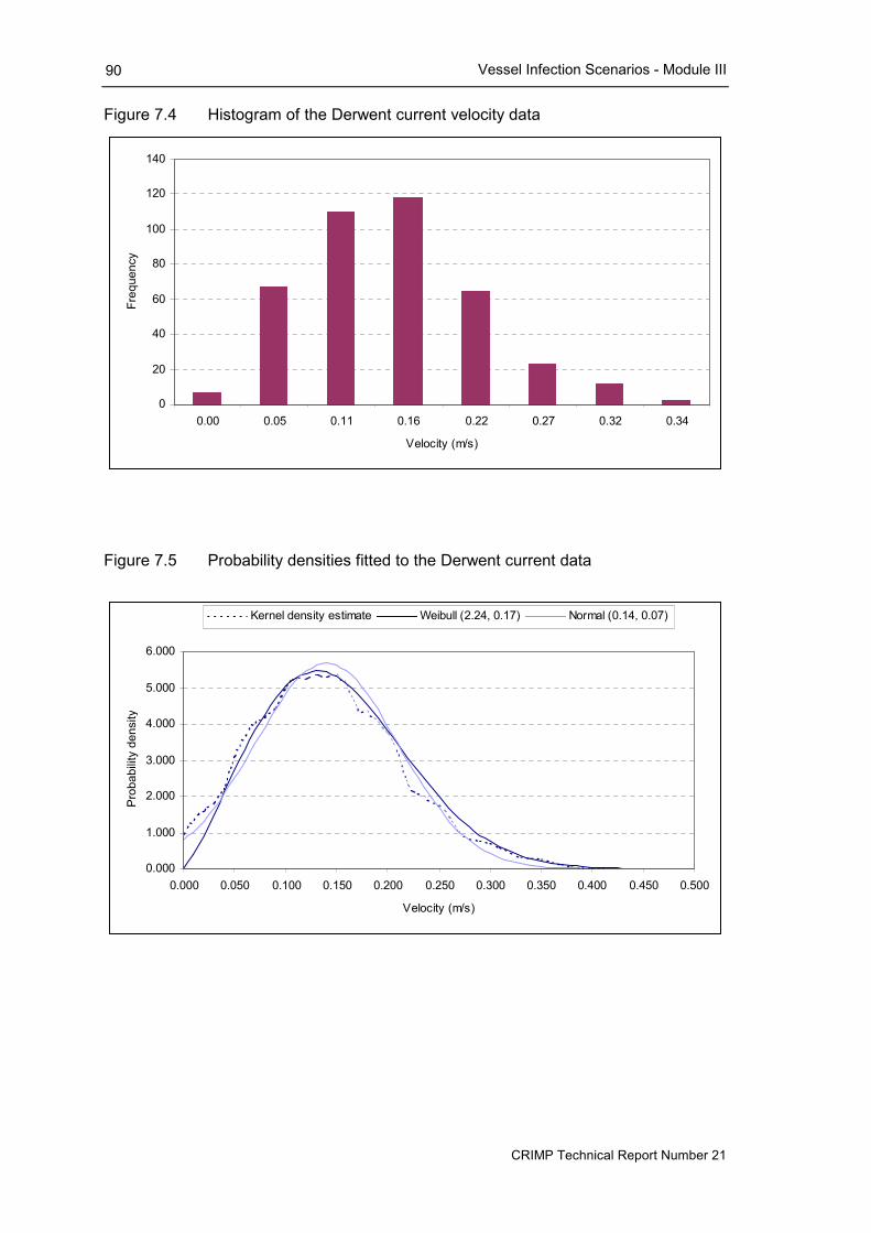
Vessel Infection Scenarios - Module III
CRIMP Technical Report Number 21
90
Figure 7.4 Histogram of the Derwent current velocity data
Figure 7.5 Probability densities fitted to the Derwent current data
0
20
40
60
80
100
120
140
0.00 0.05 0.11 0.16 0.22 0.27 0.32 0.34
Velocity (m/s)
Freq
uenc
y
0.000
1.000
2.000
3.000
4.000
5.000
6.000
0.000 0.050 0.100 0.150 0.200 0.250 0.300 0.350 0.400 0.450 0.500
Velocity (m/s)
Prob
abilit
y de
nsity
Kernel density estimate Weibull (2.24, 0.17) Normal (0.14, 0.07)

Vessel Infection Scenarios - Module III
CRIMP Technical Report Number 21
91
Figure 7.6 T values, 100 iterations of Gyrodinium uncatenatum cyst re-suspension simulation, Derwent
Figure 7.7 Propeller wash – definition sketch
Surface
Bed
1: U0 2: Zone of Flow Establishment 3: Zone of Established Flow
Hp
UxD0
θ
Dp
C 0.5Dp
0
5
10
15
20
25
30
35
40
-1 0 1 2 3 4 5 6 7 8 9 More
T value
Freq
uenc
y

Vessel Infection Scenarios - Module III
CRIMP Technical Report Number 21
92
The third zone is called the zone of established flow. The fluid flow in this region is more uniform and can be approximately described by a normal distribution whose mean decays exponentially with distance downstream. The jet velocity decreases as it entrains the surrounding fluid, causing it to spread laterally and eventually impinge on the bed.
All three zones of the propeller wash involve substantial vertical mixing which will tend to homogenise the water column, both physically and biologically, such that the probability of vessel infection is no longer a function of depth. Physical stratification and the vertical distribution of organisms will presumably re-establish at some point following the passage of a vessel. The time at which this occurs, however, remains to be determined.
The third zone of the propeller wash, and to a lesser extent the first, can cause considerable flow velocities at the seabed, thereby increasing the probability of tychoplankton infection. In contrast to its effect on a stratified water-column, the velocity profile of a propeller jet in relation to the erosion and suspension of bed material has been studied at length.
In an excellent review of the literature, Murphy (1998) notes considerable variability in the approach and results of the studies to date. Many of these studies, however, cannot be applied to real situations because they ignore the effects of the vessel’s rudder and/or the presence of quay walls and the ship’s hull. The discussion that follows is therefore largely based on the approach of Prosser (1986) who includes a number of simplifying assumptions in order to make the theory more generally applicable to real situations.
The velocity profile of a propeller wash has been variously described by many authors (see for example Verhey, 1983; Fuerher et al, 1987; Hamill and Johnston, 1993 and Ebbesmeyer et al, 1995), but essentially reduces to three equations. The axial velocity ux,r at a point x aft, and r below, the propeller is given by
( )
θ
−
=
− 2
2
a
00
r,x
xr
tan21exp
DxA
uu
, [7.19]
where A is a coefficient related to the effect of the rudder on the jet, θ is the angle at which the velocity field expands, u0 is the velocity at the face of the propeller (the efflux velocity), a is a coefficient to allow for boundary conditions and D0 is the contraction diameter. For a ducted propeller the contraction diameter is equal to the propeller diameter Dp, whereas for a non-ducted propeller it is given by
p0 D71.0D = . [7.20]
Finally, the efflux velocity is given by
Tp0 KnD6.1u = , [7.21] where n is the propeller speed (revolutions per second) and KT the thrust coefficient, a non-dimensional measure of the delivered thrust of the propeller. Prosser (1986) adopts conservative values of A = 2.8, θ = 10.20 and a = 1 (but see below), and provides typical values of KT for various values of the pitch/diameter ratio of the propeller14. Using these values the
14 Fuehrer et al (1987) provides alternative expressions for u0 if information on the thrust coefficient is unavailable.

Vessel Infection Scenarios - Module III
CRIMP Technical Report Number 21
93
zone of maximum velocity occurs between Hp/x = 0.1 – 0.25 where Hp is the height of the propeller axis over the bed.
The efflux velocity and thrust coefficients are sensitive to the velocity of the ship. However, they are also both maximised when the ship is stationary – which is assumed to be the case for vessels manoeuvring in port, with little loss of accuracy. Similarly all other currents generated by a slowly moving vessel will be small relative to the propeller wash and can therefore be ignored.
A normally positioned rudder (zero angle) has two effects on the propeller jet - it reduces the flow velocity slightly, and splits the initial propeller jet into two separate jets one of which is deflected sideways and upwards, the other sideways and downwards. Both Verhey (1983) and Fuehrer et al (1987) prescribe modifications to the coefficient A in equation [7.19] to account for the velocity loss, but the overall decrease in magnitude is small and simply ignored by Prosser (1986).
The jet deflection is caused by tangential velocity components in the initial jet, but since these are ignored in equation [7.19] it cannot provide an accurate description of the subsequent flow. Measurements made by Fuerher and Romisch (1977), however, suggest that the two jets are deflected by 120 from the propeller axis. Furthermore a rudder angle of ϕ will horizontally deflect the axis of maximum velocity by about ϕ/2, but the velocity profile is otherwise unchanged.
The presence of a solid boundary, such as a quay or berth, near a propeller jet also has a significant effect on the velocity profile of the wash. Boundaries inhibit the entrainment of fluid that ultimately ‘slows’ down the jet leading to higher velocities along the propeller axis. This can be accounted for in equation [7.19] by reducing the value of the coefficient a to 0.3 (Fuehrer and Romisch 1977). Figure 7.8, for example, shows the expected velocity at the seabed, at three berths - Risdon in Hobart Tasmania, BHP #5 in Newcastle New South Wales, and Berth # 2 at Hay Point Queensland – if the MV Iron Sturt15 berthed at these locations with a draught aft of 7m. The velocity curves are based on equations [7.19] to [7.21] with a = 1 and maximum propeller revolutions (n = 2.28). Figure 7.9 shows the same analysis with a = 0.3 to allow for the presence of a lateral boundary. The increase in predicted velocity is clearly evident.
Equations [7.19] to [7.21] were originally developed to predict propeller-induced velocities at the sea-bed. Omni-directional propellers such as ‘z’ tug-propellers or transverse bow thrusters can also be treated in this manner, allowing for the change in co-ordinate system where necessary. The same equations can also be applied to transverse stern and bow thrusters, treated as ducted propellers, such that Dp = D0. If a vessel runs its propeller astern the resulting jet will significantly influenced by the hull of the vessel – it is not clear, however, what effect this might have on subsequent seabed velocities. The combined effect of tug and vessel propeller wash could also create a very complex velocity profile. It is rare, however, for tugs to be employed along the propeller axis of a vessel whilst that vessel is berthing. The maximum seabed velocity, due to either source, should not therefore be affected.
15 Propeller diameter = 5.27m, vertical distance between keel and propeller axis = 3.37m.

Vessel Infection Scenarios - Module III
CRIMP Technical Report Number 21
94
Figure 7.8 Expected bed velocity - propeller wash of MV Iron Sturt
Figure 7.9 Expected bed velocity - propeller wash of MV Iron Sturt (lateral
boundary)
0.00
0.50
1.00
1.50
2.00
2.50
3.00
3.50
0 10 20 30 40 50 60 70
Propeller axis - x (m)
Velo
city
Ux
(m/s
)
Hobart Risdon (10m) New castle BHP #5 (13m) Hay Point Berth #2 (17m)
0.00
2.00
4.00
6.00
8.00
10.00
12.00
14.00
0 10 20 30 40 50 60 70
Propeller axis - x (m)
Velo
city
Ux
(m/s
)
Hobart Risdon (10m) New castle BHP #5 (13m) Hay Point Berth #2 (17m)
Vessel Infection Scenarios - Module III
CRIMP Technical Report Number 21
95
At level 4, Module III could use equations [7.19] to [7.21] to distinguish between ‘shallow’ and ‘deep’ ports with respect to vessel-induced tychoplankton infections. In order to achieve this, however, the assessment must access information on third-party shipping activity in the donor port, or more particularly the inter-arrival/departure times of other vessels, and their drafts. Alternatively a one-off characterisation of a port could be made on the basis of the largest vessel (at its deepest draft) that is capable of entering the port. This type of information is frequently recorded, for example in the Fairplay Ports Guide, and could provide a more objective measure of tychoplankton risk at level 1, assuming of course that technical data for this vessel was also available.
An important consideration here is the value assigned to n in equation [7.21]. The most conservative approach is to simply assign n the maximum value for the vessel concerned. However, this implies a vessel’s engines are at ‘full-ahead’ whilst berthing or entering/departing the port – which is not usually the case. An alternative approach is to define a probability distribution for n based on empirical records (easy to collect but tedious) or probability elicitation techniques (see for example Hampton et al, 1973). This would allow a more effective analysis of vessel-induced tychoplankton infections based on a distribution of propeller-induced seabed velocities, similar to that portrayed in Figure 7.4.
Finally, it is unclear to what extent the Rouse equation might be modified to allow for the effect of propeller wash. The Rouse equation was developed for ‘natural’ fluid flows in rivers, and in particular assumes that the vertical velocity-profile of the flow is parabolic due to friction with the seabed. Clearly this will not be the case if a jet is introduced at some intermediate height in the water column. The propeller wash of vessels and tugs operating in a port will also influence the ballast withdrawal envelope of other vessels in their vicinity by altering the ambient current-profile. The analyst can use the models described above to calculate the return-time of ‘still’ conditions, but what remains unclear is the time needed for the natural Rouse-type concentration profile to become re-established.
Vertical Migrator A number of benthic infauna, such as various copepods, cumaceans and ostracods, exhibit vertical migration behaviour (Brusca and Brusca, 1990). This behaviour is controlled by the same diel and tidal factors discussed in section 7.1, only in this case the organisms return to soft-sediment habitat.
The effect of vertical migration on the probability of vessel infection is much easier to model for this category of organisms because at least two of the three modeling criteria (section 7.1) are more likely to be met. By definition benthic infauna have a discrete depth-distribution, which is easily defined during periods when they are not migrating. Thus, if the migration pattern is predictable, it is possible to define periods when these organisms are unavailable to ballasting vessels, ie p(φ) = 0.05.
Clearly, this approach assumes that the seabed habitat provides a depth ‘refuge’ for benthic infauna. This may not be the case, however, in ‘shallow’ ports where the sea bed is subject to propeller-induced scour. Once the bed shear stress increases above the critical value for sediment erosion, scour will develop until the shear stress in the resulting hole falls below the threshold value. During this period benthic infauna will be introduced in the water column and thereby become available to ballasting vessels. Again the depth to which these organisms might
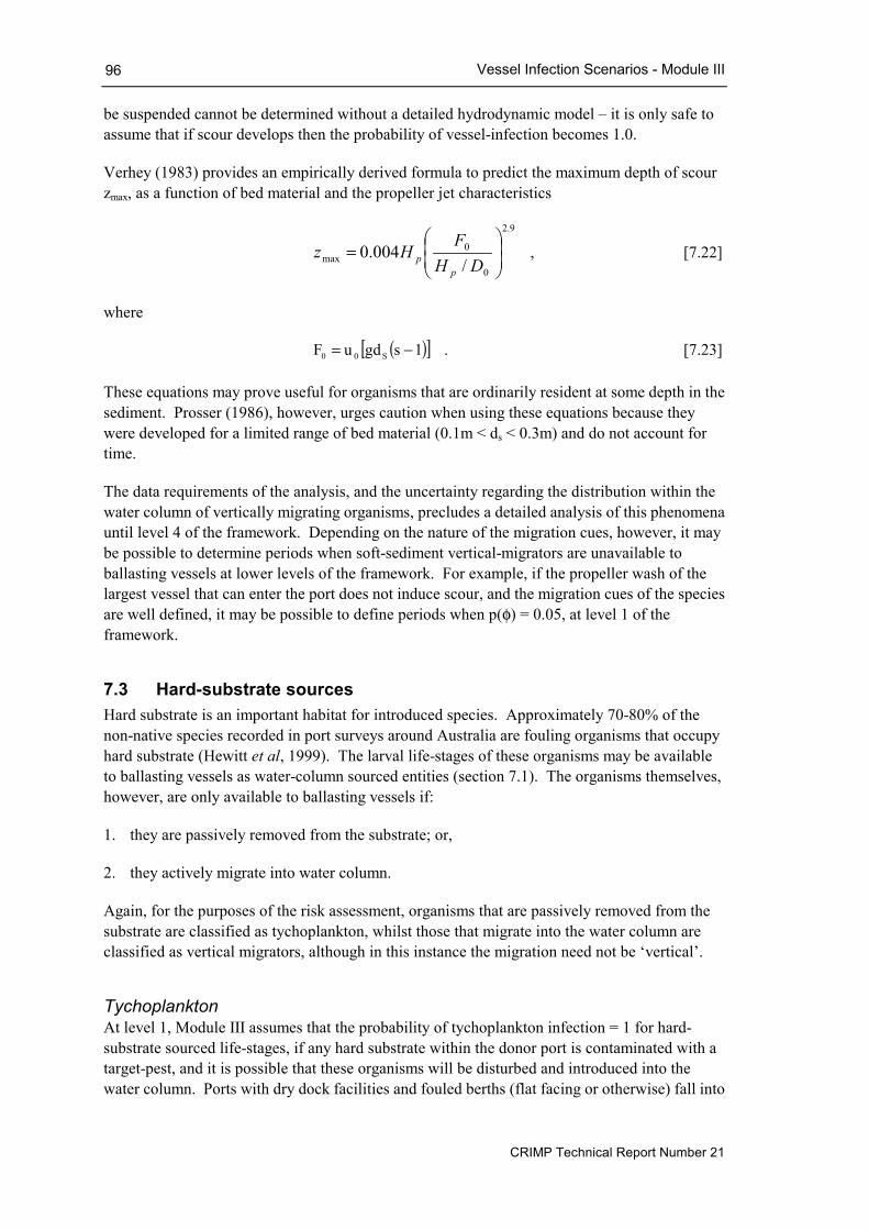
Vessel Infection Scenarios - Module III
CRIMP Technical Report Number 21
96
be suspended cannot be determined without a detailed hydrodynamic model – it is only safe to assume that if scour develops then the probability of vessel-infection becomes 1.0.
Verhey (1983) provides an empirically derived formula to predict the maximum depth of scour zmax, as a function of bed material and the propeller jet characteristics
9.2
0
0max /
004.0
=
DHF
Hzp
p , [7.22]
where
( )[ ]1sgduF S00 −= . [7.23] These equations may prove useful for organisms that are ordinarily resident at some depth in the sediment. Prosser (1986), however, urges caution when using these equations because they were developed for a limited range of bed material (0.1m < ds < 0.3m) and do not account for time.
The data requirements of the analysis, and the uncertainty regarding the distribution within the water column of vertically migrating organisms, precludes a detailed analysis of this phenomena until level 4 of the framework. Depending on the nature of the migration cues, however, it may be possible to determine periods when soft-sediment vertical-migrators are unavailable to ballasting vessels at lower levels of the framework. For example, if the propeller wash of the largest vessel that can enter the port does not induce scour, and the migration cues of the species are well defined, it may be possible to define periods when p(φ) = 0.05, at level 1 of the framework.
7.3 Hard-substrate sources Hard substrate is an important habitat for introduced species. Approximately 70-80% of the non-native species recorded in port surveys around Australia are fouling organisms that occupy hard substrate (Hewitt et al, 1999). The larval life-stages of these organisms may be available to ballasting vessels as water-column sourced entities (section 7.1). The organisms themselves, however, are only available to ballasting vessels if:
1. they are passively removed from the substrate; or,
2. they actively migrate into water column.
Again, for the purposes of the risk assessment, organisms that are passively removed from the substrate are classified as tychoplankton, whilst those that migrate into the water column are classified as vertical migrators, although in this instance the migration need not be ‘vertical’.
Tychoplankton At level 1, Module III assumes that the probability of tychoplankton infection = 1 for hard-substrate sourced life-stages, if any hard substrate within the donor port is contaminated with a target-pest, and it is possible that these organisms will be disturbed and introduced into the water column. Ports with dry dock facilities and fouled berths (flat facing or otherwise) fall into

Vessel Infection Scenarios - Module III
CRIMP Technical Report Number 21
97
this category, as would ports currently undertaking engineering activity involving fouled structures. In reality tychoplankton infections occur because fouling organisms are removed:
• mechanically through collision, abrasion or engineering activity; or
• hydraulically because of high water velocity.
In a port, mechanical removal of fouling organisms will predominantly occur due to abrasion with a hard surface. This can occur naturally, for example the effect of wave action on berth fenders, but in most case will be caused by anthropogenic activity such berthing vessels. This process is very difficult to predict, but in hindsight is unlikely to be an important infection scenario, except in cases where disused structures are subject to anthropogenic activity. All other exposed surfaces in the port that are subject to abrasion by berthing vessels are, by the routine nature of port operations, unlikely to be heavily fouled in the first place. Hull fouling is this obvious exception here, but the risk assessment framework does not currently cover this.
Disused structures which are heavily fouled and subject to periodic, but unpredictable disturbance, cannot be addressed by the risk assessment framework, except in so far as placing a minimum value (eg 0.05) on the probability of vessel infection. If structures such as these are present in a donor port, then activity around them should be carefully managed to avoid these types of infections.
In areas of a port that are routinely used, fouling organisms are more likely to be removed by hydraulic action. Furthermore since most port environments are sheltered from significant wave activity, the largest source of hydrodynamic energy will probably be the propeller wash of vessels. Fouling organisms caught in the wash of a propeller, or indeed any fluid flow, will experience three forces: drag, lift and acceleration. The lift and drag forces experienced by an organism are proportional to a representative area of the organism, whilst the acceleration force is proportional to the volume of the organism. The relative importance of each of these forces therefore depends on the size, shape and flexibility of the organism in question.
Drag is a force that tends to push objects in the direction of flow, and in high velocity flows such as a propeller wash, is due largely to the difference in pressure between the upstream and downstream ends of the organism. Drag can be modelled by the relationship
prpr,dd
d ASu21F βρ= , [7.24]
where the coefficient βd is the velocity exponent of drag, and Sd, pr is the shape coefficient of drag, defined using the profile area Apr – the organism’s area projected onto a plane perpendicular to the direction of flow (Denny, 1995).
Lift is similar to drag in that it is caused by a pressure difference between two sides of an object, but through Bernoulli’s principle, it acts in a direction perpendicular to the surface to which the organism is attached. The model for lift is similar to that of drag
plpl,ll
l ASu21F βρ= , [7.25]

Vessel Infection Scenarios - Module III
CRIMP Technical Report Number 21
98
where ρ is the density of seawater, u is velocity, βl is the velocity exponent of lift and Sl, pl is the shape coefficient of lift, calculated on the basis of the planform area Apl – the organism’s area projected onto the surface to which it is attached.
Lift is often larger than drag because for most fouling organisms the planform area is much larger than the profile area. Lift however, only occurs when the material beneath an organism is capable of transmitting a hydrostatic pressure. Thus a mussel bed in a fluid flow will experience lift because of the difference in hydrostatic pressure between the fluid under the bed and that over it, whereas an acorn barnacle will not because it attaches to surface using a solid glue (Denny, 1995).
The force of acceleration acts along the direction of flow and is proportional to the volume of water displaced by an organism. For a stationary, inflexible object, situated in an accelerating flow, the acceleration force is typically given by
VaCVaF aa ρ+ρ= , [7.26] where V is the volume of fluid displaced by the organism, a is the acceleration of the fluid and Ca is the dimensionless added mass coefficient. For an object with a constant added mass coefficient, equation [7.26] is commonly simplified to
VaCF ma ρ= , [7.27] where Cm = (1 + Ca) is the inertia coefficient (Gaylord et al, 1994). Bluff-shaped fouling invertebrates generally displace very small volumes of fluid and have a small added mass coefficient. The acceleration force they experience is therefore negligible compared to the drag and lift forces, and are commonly ignored (Denny, 1995). Thus for these organisms the total force they experience is approximately the vector sum of lift and drag
( )21
2l
2d FFF += . [7.28]
By contrast algae tend to displace much higher volumes of water, have higher added mass coefficients and deform under a velocity field thereby minimising lift (Gaylord et al, 1994). Thus in flows capable of deforming algae, lift is negligible compared to drag and acceleration. Thus for algae the total force they experience is approximately the sum of drag and acceleration
ad FFF += , [7.29] an expression known as the Morison equation. In this context, however, the calculation of Fd is complicated because the organism is capable of deforming and becoming more streamlined, such that its drag coefficient decreases, with increasing velocity. Under high flows (10–20 m/s), however, the drag coefficient reaches an asymptotic minimum which is effectively constant for the species concerned.
In order to calculate the probability of tychoplankton infection, the analyst must compare the maximum hydrodynamic force that a fouling organism will experience, based for example on the efflux velocity of the propeller, with the dislodgment force Fp needed to remove the organism from the hard-substrate. Dislodgment force is commonly modelled as a function of the size of the organism

Vessel Infection Scenarios - Module III
CRIMP Technical Report Number 21
99
3AF 21pαα+α= . [7.30]
where A is the characteristic area of organism – typically the planform area for a fouling invertebrate or the projected area for algae. The coefficients α in this relationship must be determined empirically by measuring the dislodgment force and fitting the results to the model. Gaylord et al (1994) fits a modified Weibull distribution to describe interspecies variation in the coefficient α2 and α3, whereas Denny (1995) uses an extreme-value distribution to model this variation.
The velocity exponent, shape coefficients and added mass coefficients employed in equations [7.26] to [7.29] can be easily measured in a flow tank or wind tunnel. Denny (1995) provides values of these coefficients for a wide variety of inter and sub-tidal fauna. In virtually all cases the velocity exponents of lift and drag are very close to 2.00. Furthermore because the shape coefficients are similar for organisms that are similar in size and shape, the values provided by Denny (1995) can be used as look-up tables for other organisms using basic information on the size and shape, or even a simple photograph.
Gaylord et al (1994) provide added mass coefficients for only three species of intertidal algae, and note that this parameter is very sensitive to the size, morphology and deformation properties of the species concerned. This parameter is clearly very species-specific and must therefore be determined by laboratory measurements on a case-by-case basis. Similarly the coefficients in equation [7.30] cannot be reliably predicted on the basis of prior knowledge of the species characteristic area – the average ‘strength’ of individuals are known to vary dramatically between species, as does the shape of the distribution that describes the variation within the species.
The ‘strength’ of a fouling organism may also vary according to a variety of other factors including:
• seasonality (see for example Price, 1980);
• physio-chemical stress;
• the substrate to which the organism is attached, see for example tychoplankton risk for epiphytes; and,
• for algae at least, nicks or surface flaws on the organism.
From a risk assessment perspective, this last factor is particularly significant because portions of a plant, containing spores or gametes, may be broken-off with energy much lower than that required to remove the whole plant16. Furthermore these portions will be much smaller than the whole plant and therefore much more likely to pass through the ballast water sea suction strainer. Without a much more detailed examination of this process, the tychoplankton risk of adult/juvenile algae must by considered to be 1.0 for those species where this infection scenario is plausible.
16 Denny et al (1989) note that macro-algae are biologically ‘brittle’ but can avoid catastrophic fracture at sites where they are damaged, up to a point, by deforming, lowering the aspect ratio of the flaw and thereby reducing the concentration of stress in this area.

Vessel Infection Scenarios - Module III
CRIMP Technical Report Number 21
100
So again, whilst the theory of tychoplankton risk for hard-substrate sourced life-stages is relatively well developed, the data requirements preclude a quantitative assessment of this risk at the lower levels of the risk assessment framework. Accordingly module III will not model tychoplankton risk for hard-substrate sourced life-stages until level 4.
Vertical Migrator A few organisms that inhabit hard substrate are known to undertake ‘vertical’ migrations. Carlton et al (1995) for example describes the behaviour of the wood-boring gribble, Limnoria spp. that inhabits wooden structures in ports but undergoes nocturnal ‘migrations’ by swimming between structures.
Each of the criteria in identified in section 7.1 must be met in order to model this phenomenon. In these circumstances, however, the hard-substrate may have a vertical and horizontal distribution and the migrations themselves need not be ‘vertical’. Despite these complications the modelling process could be simpler because hard-substrate usually provides a distinct ‘refuge’ similar to, but more immutable than, the sediment ‘refuge’ noted in section 7.2.
At level 1, module III will simply assume that hard-substrate vertical-migrators are uniformly available to ballasting vessels, ie p(φ) = 1.0. At level 4 a more detailed analysis will be performed if the criteria stipulated in section 7.1 can be met.
7.4 Epiphyte sources Epiphytic organisms (organisms that are attached to another organism) are only available to ballasting vessels if:
1. they are passively removed from the host;
2. they actively migrate from the host; or
3. the host to which they are attached is entrained into the ballast tank.
Again, for the purposes of the risk assessment framework, epiphytic organisms that are passively removed from their origin are referred to as tychoplankton. Epiphytic organisms that migrate into the water column are referred to as vertical migrators, but the migration need not necessarily be ‘vertical’. Finally epiphytes that are entrained into the ballast tank as ‘hitch-hikers’ on another organism are referred to as ‘floating detached’ after Carlton et al (1995).
Tychoplankton The mechanics of epiphyte tychoplankton-infections are essentially identical to those described in sections 7.2 and 7.3. As a first approximation, the likelihood of infection is a function of the forces acting to remove the organism from its host, and the ‘strength’ of the organisms to withstand these forces. In this context, however, the assessment must verify whether the dislodgment force needed to remove the organism from its host is greater than that needed to remove the host from its substrate, leading to a ‘floating-detached’ infection scenario (see below). At level 1, Module III will simply assume that the probability of vessel-infection for epiphyte target-species is 1.0, if these species are present in the donor port. At level 4, however, a detailed analysis of tychoplankton risk will be undertaken using the equations developed in

Vessel Infection Scenarios - Module III
CRIMP Technical Report Number 21
101
sections 7.2 and 7.3. Again this level of analysis requires large amounts of species, and vessel specific information, some of which can only be determined empirically.
Vertical Migrator At level 1, Module III will assume that epiphyte life-stages that ‘vertically’ migrate are uniformly available to ballasting vessels, ie p(φ) = 1.0. If the data requirements and modelling criteria listed in section 7.1 are met, then a more sophisticated level of analysis will be conducted at level 4.
Floating Detached A floating detached infection scenario occurs when the dislodgment force of the epiphyte exceeds that of the host. In these circumstances the probability of epiphyte infection is calculated using the host as the target organism, with some important provisos:
• fracture of the host may occur before the flow velocity is sufficient to remove the host from its substrate;
• some allowance must be made for the influence of the epiphyte on the physical properties of the host, particularly its sinking velocity and drag coefficient; and,
• the target organism size becomes size plus host, fractured or otherwise.
Again this type of analysis cannot be conducted until level 4 of the assessment framework.
7.5 Other infection scenarios The fault-tree analysis identified four less tractable infection scenarios:
• ballast tank populations – species that reside and reproduce in the ballast tank, such that the vessel becomes an infectious unit;
• ballast water carry-over – caused by multiple ballast sources in a tank or because of unpumpable ballast;
• crevicolous species – species which actively shelter in crevices and holes; and,
• third-party infection scenarios – vessel infections in ports that are themselves uninfected because of the ballast-water discharge or hull fouling of another infected vessel.
At level 1, the risk assessment framework can flag vessels that may contain ballast tank populations. Beyond this an assessment of risk could be made for those life-stages that are small enough to leave the ballast tank. This type of analysis would be conducted at level 3 by calculating p(υ), but assuming p(ψ) = 1.0. By archiving the ballast report forms, the framework is able to determine the age of unpumpable ballast and therefore the risk associated with ballast water carry-over, using a journey-survival model, at level 2 (see next section). The framework does not currently cater for crevicolous species – none of the species on the current target list exhibit this type of behaviour. Finally, the framework may be able to estimate the probability of third-party infections, but only with a very sophisticated analysis such as that envisaged at level 5.

.
Journey Survival - Module IV
CRIMP Technical Report Number 21
103
8 JOURNEY SURVIVAL (MODULE IV)
Module IV has four objectives:
1. to undertake a simple journey-competency test;
2. to model the survival of target-species as a function of journey time;
3. to model the effect of the ballast pump on journey survivorship; and,
4. to model the effect of ballast management strategies on journey survivorship.
8.1 Competency test The journey-competency test is conducted on those life-stages that are small enough to enter the ballast tank. The test allocates a score to those species that are capable of creating ballast tank populations, eg fouling species or benthic species. The score provides a simple measure of the likelihood of a ballast-tank population, given by
1score0period competency
durationjourney score ≤≤= ,
where the competency period is defined as
∑=
−=j
1ii stagelifedurationperiod competency . [8.1]
where j is the number of life-stages that are small enough to enter the ballast tank, up to and including the life-stage that normally settles out of the water column. If the species score is greater than 1.0 then a warning is issued to the analyst about the possibility of a ballast-tank population. This cut-off value is arbitrary and can be easily altered to flag-up more or less vessels.
The competency test assumes that the probability of the species commencing its life-stage is uniformly distributed throughout the period that it is available to ballasting vessels. It is only intended to be a simple hazard score to flag vessels that may have ballast-tank populations. The score is not incorporated into the hazard ranking of the vessel, and plays no further part in the risk assessment calculations.
For most dinoflagellate species, the competency test will always return a very low score. This is because the competency period for most cysts is very long in relation to a typical journey. However, this is consistent with evidence to date that suggests that dinoflagellates will not establishing reproducing populations within a vessel because the motile life-stages rapidly perish in the ballast tank (Hallegraeff, 1998).

Journey Survival - Module IV
CRIMP Technical Report Number 21
104
8.2 Journey survivorship To date relatively few studies of journey survival have been completed. This is probably because such studies are time consuming, particularly in terms of sorting and counting samples, and are often costly to conduct. The results of some studies that have been completed (Table 8.1), however, suggest that most organisms in a ballast tank will eventually die.
Carlton et al (1995) suggest that mortality in the ballast tank occurs because of:
• biological alterations – including predation by other organisms and decreased food supply;
• physiological limitations – particularly the absence of light or suitable substrate to settle on; and,
• physical-chemical conditions – temperature changes, oxygen decline and water contamination due to pollutants or shipboard contaminants.
A variety of taxa, however, are well adapted to survival in a ballast-tank environment. These may include taxa which produce cysts or ‘resting’ stages or eggs, taxa with larvae that do not feed or are lecithotrophic17, or taxa with larvae that are capable of delaying metamorphosis in the absence of a suitable settlement site (Carlton, 1985).
The second objective of Module IV is to model the mortality that occurs in the ballast tank during the vessel’s voyage. These models are employed at level 2 of the framework to provide the first quantitative measure of ballast-water risk. The most immediate problem in this context is the absence of information on size of the initial inoculum. Without this information the analyst is unable to specify the problem in terms of traditional birth/death population dynamics. Furthermore this type of information is unlikely to be available without a very detailed analysis, such as that envisaged at level 5 of the risk assessment framework. This problem can be avoided by modelling the mortality process in terms of the survival of individuals in a population. In this approach the length of time that an individual is expected to survive in the ballast tank (its ballast life expectancy - L) is viewed as a random variable. The aim of the model is to then estimate the probability that L exceeds the journey duration, implying that some proportion of the original inoculum is still alive at the end of the vessel’s journey. Hayes (1998) provides an example of this approach for Asterias amurensis. However, this approach cannot be adopted for species that actually increase in abundance, as noted on one occasion for the benthic harpacticoid copepod Tisbe graciloides (Table 8.1).
Having specified the problem in terms of a random variable L, the analyst needs to determine the type of distribution that best describes this variable, and the parameters of this distribution. At this stage the framework assumes that the distribution is species-specific, meaning the same distribution describes all intra-species variation associated with different voyages. It is clear from Table 8.1 that most of the taxa studied to date decline during the vessel’s voyage, and in some cases the rate of decline is rapid. For these taxa L might be modelled as an exponential random variable. In many other cases, however, particularly over shorter voyages, the rate of decline varies, with no clear overall pattern.
17 Non-feeding larvae that utilise yolk as a source of nutrition.

Journey Survival - Module IV
CRIMP Technical Report Number 21
105
Table 8.1 The results of some journey survival studies
AUTHOR
VOYAGE DETAILS
BIOLOGICAL GROUP
MODEL TYPE
Wonham et al, (1996)
Vessel = MV Leon Start = Hadera, Israel End = Baltimore, Maryland Duration = 18 days
Zooplankton Phytoplankton Copepods Gastropods Bivalves Polycheates
Exponential decline Exponential decline Exponential decline Linear decline Unclear but declined Unclear but declined
Gollasch et al, (1998)
Vessel = DSR America Start = Singapore End = Bremerhaven, Germany Duration = 23 days
Copepods Diatoms Tisbe graciloides
Exponential decline Exponential decline Unclear but increased
Rigby et al, (1997)
Vessel = MV Iron Whyalla Start = Port Kembla, Australia End = Port Hedland, Australia Duration = 11 days
Copepods Chaetognaths Polychaetes Ostracods
Exponential decline Exponential decline Unclear but declined Unclear but declined
Murphy, (1997)
Vessel = MV Iron Sturt Start = Hobart, Australia End = Geelong/Port Pirie, Australia Duration = 4 – 6 days
Bivalve larvae Crab zoea Crab megalope
Exponential decline Exponential decline Unclear but constant
Sutton (unpub data)
Vessel = MV Iron Sturt Start = Hobart, Australia End = Newcastle, Australia Duration = 5 days a
Bivalve larvae Polychaetes Crab zoea Gastropods Asterias larvae
Exponential decline Unclear but declined Unclear but declined Unclear but declined Unclear but constant
Sutton (unpub data)
Vessel = MV Iron Sturt Start = Hobart, Australia End = Port Pirie, Australia Duration = 9 days
Bivalve larvae Polychaetes
Unclear but declined Unclear but declined
a = refers to the period over which samples were taken, actual journey duration exceeds 5 days.

Journey Survival - Module IV
CRIMP Technical Report Number 21
106
Having specified an appropriate model for L, the next problem is to estimate the value of the parameters of the distribution, for example the death rate in an exponential model. En-route sampling studies are the only way to achieve this - taking ballast samples during the voyage, plotting the change in abundance and then fitting a Bayesian or classical statistical model to the results. The sample size for these models, however, is likely to be low because of the time needed to complete survival studies. This can be partially offset by:
• treating individual ballast tanks, such as port and starboard, as statistically independent during a study;
• using rapid identification techniques, using genetic markers for example, to reduce the time and cost of survival studies18; and,
• using Bayesian statistical models that can be easily updated as more information is made available.
Bayesian statistical models can also be updated by taking ballast samples at the end of the voyage and recording those species that are still alive, ie their life-expectancy is at least equal to the age of ballast water concerned (see Hayes, 1998 for further details). Ballast samples taken at the end of a voyage, however, do not provide any information on those species that perished during the voyage. Thus these types of samples can only be used to ground-truth survival models in one direction.
Ideally the journey survival analysis should be conducted for each life-stage of the species that is small enough to enter the tank. This would entail a separate survival model and/or parameters for each life-stage. The overall probability of journey survival for the species is then given by
( ) ( )[ ]∏=
−−=m
rrpp
1
11 ψψ , [8.2]
for the life-stages (r = 1 to m) of the target species that can enter the ballast tank. In reality, however, journey survival data may only be available for a limited set of the life-stage of a species, for example all the larval life-stages. Indeed the mortality rates measured in the field will probably represent a mixed distribution of all life-stages of the species that were present in the ballast tank at the start of the journey. This does not present any problems to the risk assessment process, so long as the analyst is able to identify the life-stages that belong to the distribution.
8.3 Ballast pump effects During survival studies onboard the MV Iron Sturt, Murphy (1997) recorded very high mortality of zooplankton at the start of the journey, and suggested that this may be attributable to the effect of the ballast pump, or the hypochlorite treatment at the sea chest. Similarly Gollasch et al (1998) suggest that the effects of the ballast pump might have caused the initially high mortality they witnessed.
18 A number of such techniques are currently available (eg Evans et al, 1998; Murphy and Goggin, 1997).

Journey Survival - Module IV
CRIMP Technical Report Number 21
107
The effect of the ballast pump on the subsequent survival of organisms is currently unclear. Carlton et al (1995) note that ship’s ballast pumps are usually high volume, low pressure systems that are not designed to achieve very high velocities, and are therefore unlikely to have a significant effect on the subsequent survival of organisms in the ballast tank. Rigby et al (1997) note that phytoplankton retrieved from fire hose outlets onboard the MV Iron Whyalla, were in poor condition relative to those collected by bucket. The pressure developed within a fire hose pump, however, are normally much higher than those developed in the ballast system.
Despite this there is other evidence to suggest that the turbulence generated by the ballast pump has an adverse effect on the survival of plankton. For example, Thomas and Gibson (1990) note that some species of dinoflagellates are very sensitive to turbulence, to the extent that growth is inhibited if culture flasks are shaken. Similarly Pearson et al (1989) demonstrated increased mortality of paddlefish at current velocities as low as 1.5 ms1, and that mortality was a direct exponential function of current velocity. Similar results were also observed for fish eggs.
The importance of the ballast pump on the subsequent survival of organisms is clearly species-specific. This phenomenon has not been investigated, however, in a controlled and quantitative manner. Initial studies undertaken by CRIMP are as yet inconclusive (pers comm C. Sutton). Module IV will incorporate any differential mortality rate between gravity fed and pumped organisms, as and when there is sufficient information to do so. Prior to this, problems may arise if a ballast tank is filled using gravity feed, but the journey survival model is based on a mortality rate measured in a tank filled by the pump. In practise, however, most tanks are filled using both gravity and pump feeds. Thus again, most field measurements will record a mixed mortality distribution that is quite sufficient for the purposes of the risk assessment.
8.4 Management strategies Carlton et al (1995) lists a variety of active and passive ballast-management techniques that vessels might employ whilst en-route. Module IV will ultimately aim to incorporate the effects of these techniques into the analysis of journey survival. In order to do this, however, the effectiveness of these techniques must be expressed in a manner that is compatible with the survival model. For example the efficacy of ballast exchange is often cited in terms of the reduction in number of species, or number of individuals (see for example Locke et al, 1993). Unfortunately this type of information sheds no light on the change in death rate of individual species, and cannot therefore be used by a model based on the expected value of L.
If the efficacy of alternative ballast management strategies is expressed in a suitable format, such as an increased death rate, then this can be readily incorporated into Module IV as an additional component of the journey survival analysis. This type of analysis will lay the necessary foundation of a risk-benefit analysis of ballast-management options. As it currently stands, however, Module IV (and indeed the framework) conservatively assumes that the vessel does no implement any ballast management strategies.

.

Inductive Hazard Assessment
CRIMP Technical Report Number 21
109
9 INDUCTIVE HAZARD ASSESSMENT
The sequence of events that lead to a successful ballast-water invasion, like all bio-invasion processes, are complex and difficult to predict. The fault-tree analysis described in Hayes and Hewitt (1998) decomposes this complexity into a series of logical steps. The modules described in the three previous sections of this report are designed to measure the probability of success at each of these steps. It is important to emphasise, however, that bio-invasion processes are not time invariant. Carlton (1996) makes this point well, listing six scenarios that can lead to a successful invasion, including:
• environmental changes in existing donor region, including the introduction of new species into existing regions, eg donor ports;
• environmental changes in the recipient region, eg recipient ports;
• an invasion window opens as the proper combination of conditions happens to coincide; and,
• dispersal vector changes, including the emergence of new vector.
In light of this, the risk assessment framework must be able to continually monitor the processes and conditions that occur in the donor port, the vessel and the recipient port. This on-going hazard assessment is best implemented by on-site measurement of these conditions and processes. It is clearly impractical, however, to continually monitor all anthropogenic and natural processes that occur in a port or the vessels that operate in them. The objective of this section of the report is to describe techniques that will help identify bio-invasion hazards in advance, so that they can be flagged for regular or continual assessment.
The domain of this analysis includes all processes and operations within the port that could potentially influence the port environment, the distribution of pest species within that environment, and the vessel-infection scenarios described in section 7. In particular the analysis focuses on:
• variation in natural environmental parameters such as tidal current flows, wind and wave induced shear stress, salinity and temperature;
• the ballasting and berthing processes of vessels; and,
• the effects of any other anthropogenic activity such as dredging, berth construction or hull cleaning operations.
These processes can be addressed through environmental distribution functions, inductive HAZOP analysis or both.

Inductive Hazard Assessment
CRIMP Technical Report Number 21
110
9.1 Environmental distribution functions Section 6 of the report discussed a variety of statistical techniques that will capture the environmental variation in a donor or recipient port. It was noted, however, that the utility of these techniques is dependent on the quantity and quality of data relative to the spatial and temporal variability of the port environment.
Ideally each of the natural parameters that influence the probability of invasion will be completely described by probability density (or mass) functions over monthly intervals. This description should extend to the physical and biological characteristics of the port, and also allow the potential influence of the extremes of these distributions to be investigated. For example, under extreme tides the induced shear stress at the sediment/water column interface may be significantly altered, thereby influencing the availability of pest species that reside in the benthos. If this is deemed significant the analysis should strive to determine return periods for these tidal currents. Similar considerations can be applied to temperature, salinity, or even wind and wave conditions.
This approach, however, pre-supposes high resolution time series data are available for each environmental parameter within each port. Furthermore it requires that these time series extend back many years in order that events of a low return period are captured. Furthermore if a fundamental change of conditions is not recorded within the data set, the distribution function will not adequately reflect the true environmental variability. For example, Gaines and Denny (1993) note that EV distributions developed for wind speed in areas prone to hurricanes will underestimate maximum velocity if the original time-series data do not include hurricane events. In this example hurricanes represent the ‘fundamental change in conditions’.
An alternative qualitative approach, facilitated by the fault tree analysis, is to identify the necessary conditions for a bio-hazard within a particular port, and ask whether these conditions are actually feasible in the environment concerned. This process can be formalised in a HAZOP type analysis that aims to investigate the effects of deviations from ‘average’ or ‘normal’ conditions in relation to the transport and survival of specific marine pests.
9.2 Port and vessel based HAZOP analysis
What is HAZOP? There are essentially four ways to identify hazards. In the first instance the assessor can simply list the obvious hazards. Alternatively one can wait and observe what happens, an effective but hardly precautionary approach. The third option is to develop a series of checklists based on the experience of the assessor perhaps in conjunction with a fault tree analysis. Checklists of this type are usually most effective for systems which are well understood but have the disadvantage that items not on the list are not brought forward for consideration and thus checklists are not well suited to novel systems and processes. Under these circumstances Kletz (1986) recommends a more creative and open-ended approach, described in industrial systems as hazard and operability or HAZOP analysis.
HAZOP is a technique that encourages a group of assessors familiar with the system in question to apply foresight and imagination, in an inductive but formalised and rigorous way, to identify potentially hazardous situations. In an industrial context the procedure takes as its starting point the line, flow and control diagrams that represent the intended operating system of the plant.

Inductive Hazard Assessment
CRIMP Technical Report Number 21
111
The technique then systematically works through each item of plant, for example a pipeline leading from a feed vessel to a reactor, and applies guide words such as more, less, other than, etc. to focus attention on possible deviations from the planned intention. When studying batch plant the guide words are applied to the instructions as well as to the individual components of the plant. Each application of the guide word usually generates a number of potential deviations from intent, from which possible causes and consequences are identified and recorded, as illustrated in Figure 9.1.
HAZOP is successful because it is systematic and also because it makes no prior assumptions as to the potential likelihood of hazard scenarios. It is therefore an excellent means to identify plausible, but low probability, events that may ordinarily be overlooked simply because they do no form part of the assessors established operating experience.
Despite its success, HAZOP has not been widely adopted outside of an industrial context. Indeed for risks associated with environmental issues its use has only been advocated in one other context, namely for the manufacture and release of genetically modified organisms (refer to Hayes, 1997). It seems apparent, however, that unexpected interactions and processes are equally as likely to give rise to hazards in complex environmental systems as in complex industrial plants. This would therefore seem to warrant the extension of HAZOP techniques to these systems.
In this context, the objective of a HAZOP analysis is to identify hazards in relation to the survival and uptake (by vessels) of target-species in a port, as indicated by the fault tree analysis (Hayes and Hewitt, 1998). A suggested set of guide words specifically designed to address ballast water risks is provided in Table 9.1. Having applied the guide words to each of the relevant procedures and processes a series of deviations are generated. In certain instances these deviations may need to be considered in conjunction with other events, particularly in relation to the interaction between anthropogenic activities and natural processes, and a specific guide word is provided to trigger this.
Having applied the guide words the assessment goes on to consider the potential consequences of the deviations and potential combinations elicited by the approach, and decides whether they are likely to alter the hazard status of a port, in relation to the survival of pest species or their entrainment. If the extent of the alteration is significant then further assessment is needed in terms of expected frequency or specific action to prevent the hazard occurring. This process is anticipated to be quite labour intensive in the first instance, but if performed properly need only be undertaken once for each port and each of the vessel categories identified in Table 9.2. The analysis should be repeated, however, in the event that the port undergoes a significant modification such as the building of a new berth. The application of HAZOP techniques to ballast water risk assessment is entirely new and untested. It is recommended therefore that a test run of a port based HAZOP analysis be held to confirm its efficacy.
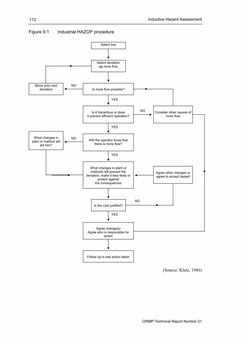
Inductive Hazard Assessment
CRIMP Technical Report Number 21
112
Figure 9.1 Industrial HAZOP procedure
Select line
Select deviationeg more flow
Is more flow possible?
Is it hazardous or doesit prevent efficient operation?
Consider other causes ofmore flow
Move onto nextdeviation
Will the operator know thatthere is more flow?
What changes in plant ormethods will prevent the
deviation, make it less likely orprotect against
the consequences
What changes inplant or method will
tell him?
Is the cost justified?
Agree change(s)Agree who is responsible for
action
Follow up to see action taken
Agree other changes oragree to accept hazard
NO
YES
NO
YES
NO
NO
YES
YES
(Source: Kletz, 1986)

Inductive Hazard Assessment
CRIMP Technical Report Number 21
113
Table 9.1 Suggested HAZOP guide words for ballast-water risk-assessment
GUIDE WORD MEANING None A complete negation of the intent - the process or procedure simply does not take place; eg
freshwater input to port environment ceases.
More of A quantitative increase in any relevant physical or biological property; can also be applied to time to express an increase in the duration of a process or its frequency; eg pest spawning population higher than expected
Less of A quantitative decrease in any relevant physical or biological property; can also be applied to time to express a decrease in the duration of a process or its frequency; eg seabed tidal current lower than anticipated
As well as Something additional to the process under consideration occurs - used to investigate the effect of possible combinations of environmental and/or anthropogenic processes; eg pier extension occurs during a period of high seabed current conditions
Part of Something less than expected occurs - used to investigate the effect when only part of a planned combination of events occurs; eg only part of a vessels intended loading and ballasting plan is completed
Other than Something quite different to the planned or anticipated process takes place; eg a periodic dredging operation does not take place
Where else
An intended event or process takes place in a location other than anticipated or expected; eg a vessel berths at a different location within the port
When else
An intended event or process takes place at a different time to that anticipated or expected; eg a vessel berths at a different time to that anticipated.
Table 9.2 Suggested vessel categories for HAZOP analysis
VESSEL RELATED VESSEL TYPES 1. General cargo 2. Container ship 3. Tanker 4. Bulk carrier 5. Passenger ship 6. Vehicles carrier
Refrigerated cargo Oil tanker, chemical, tanker, liquefied gas/chemical tanker (LPG or LNG), other tankers (water, wine, fruit juice etc.) Wood chip carrier, cement carrier, ore carrier, ore/bulk/oil carrier, ore/oil carrier Ferry, Passenger/RORO cargo

Inductive Hazard Assessment
CRIMP Technical Report Number 21
114
HAZOP for natural port processes A HAZOP analysis for the natural processes that occur in a port environment is predicated on being able to identify the environmental equivalent of the industrial process of intent, in other words the environmental parameters and biological processes that influence the survival, dispersal and entrainment of pest species. The models used in the higher levels of the framework, for example the survival and vessel-infection models, should identify the relevant processes. The HAZOP should not be applied therefore until these levels are reached, ie from level 2 or 3 onwards. The hazard identification procedure is formalised by considering the biological and physical parameters designated in these models and applying the guide words to them. Some consideration should also be given to the potential effects of interaction between deviated biological and physical conditions. The guide words ‘as well as’ is provided to specifically trigger this.
Table 9.3 provides a tentative example of the type of outputs a HAZOP analysis for port environment conditions might develop. Guide words are applied to model parameters to identify possible ‘deviations’. In each instance the significance of the deviations is gauged in light of the tolerance criteria identified for survival of the species and the entrainment criteria developed through the fault tree analysis. The scope of the analysis can be made more manageable, in the first instance, by only applying the process to ports which have been designated as nominally ‘safe’ because the species in question fails either the survival criteria or entrainment criteria. Clearly in these circumstances the assessor is particularly interested in those criteria which the species failed on, and possible deviations within the port and species itself which could lead to a ‘pass’ on these criteria.
HAZOP for berthing and ballasting processes Shipping operations within ports are usually governed by Standard Operating Procedures (SOP’s). The port of Newcastle for example has published Ship Handling Safety Guidelines that detail the tug requirements and berthing/removal procedures for various categories of vessel at various times. Within the bounds of these procedures, however, the actual berthing and ballasting procedures are characterised by a high degree of uncertainty - the operation that takes place is ultimately at the discretion of the pilot or master.
This uncertainty makes it very difficult to identify a specific ‘process of intent’ for HAZOP purposes beyond descriptions such as vessel berths, deballasts and loads. This same uncertainty, however, makes it all the more important that the assessment is able to test for conditions under which potential hazards may arise. Furthermore the uncertainty in the process is largely due to the individual behaviour of the skipper or pilot responding to a multitude of factors such as the weather conditions, tide, vessel draft, trim and cargo, and as such is much less amenable to statistical treatment.
These comments notwithstanding, it is possible to identify a minimum set of actions that completely describe the behaviour of a vessel within a port and thereby provide the basis for a HAZOP type analysis. Any SOP’s that are practiced in the port will help to identify this set, which should include the following elements:
• ENTRANCE - used to designate the vessels entry into the port environment, at which point the vessel usually picks up a pilot;

Inductive Hazard Assessment
CRIMP Technical Report Number 21
115
Table 9.3 Example of HAZOP analysis for natural processes
GUIDE WORD
DEVIATION POSSIBLE CAUSE CONSEQUENCE & SIGNIFICANCE ASSESSMENT
None Salinity – no freshwater
Drought Consider likelihood and effects of drought conditions on port environment in relation to species tolerance for salinity, temperature, etc. and port circulation patterns
More of Temperature – increased
Simply a warm year Test derivation of EV distribution for SST – time-series length relative to other meteorological records, presence of trend
Localised warming, eg industrial outfall
Check for presence of industrial outfalls at temperatures significantly higher than ambient
Localised warming due to lagoon effect
Check for presence of partially enclosed habitats with restricted water circulation
Oxygen – increased
Reduction in detritus input
Check for evidence of reduction in detritus loads and variation in oxygen minima at the freshwater-brackish water interface, relative to species tolerance
Less of Salinity – reduced
Increased freshwater input into areas of restricted circulation
Check for presence of partially enclosed habitats with restricted circulation and freshwater input, together with extremes in freshwater discharge history
Stratified flow regime within estuary
Check for evidence of salt wedge and freshwater lens, variation in relation to freshwater input, and the extent to which this is captured in port data
As well as
Bed shear stress – increase
Sympathetic effect of extreme tidal current and wind induced shear stress
Hypothesise potential maximum shear bed stress conditions (and likely return period) on basis of sympathetic extremes of tide and wind, highlighting likelihood distribution in time
Target species presence – altered behaviour
Predation avoidance responses between target species
Consider any evidence for behavioural interactions between target species and implications for vessel infection models – eg altered vertical migration patterns
Where else
Salinity – altered circulation
Flood events change pattern of freshwater sources
Consider likelihood of new freshwater (or storm drain) inputs into port environment and likely significance with respect to circulation and salinity/temperature regime
Target species – altered distribution
Settlement or colonisation of new areas in port
Consider availability of existing and new habitats within port and potential implications for pest distribution
When else
Altered reproductive season
Species hypothetical niche is broader than realised niche
Consider any evidence for species reproductive season extending either side of documented season in native or introduced range

Inductive Hazard Assessment
CRIMP Technical Report Number 21
116
• TRANSIT - the vessel’s route and usual behaviour from the entrance of the port to its allocated berth;
• BERTHING - the actual berthing process often entailing the use of tugs to assist the vessel in manoeuvring or to maintain its position in relation to the berth;
• (UN)LOAD & (DE)BALLAST - the majority of the ballasting or de-ballasting process occurs at the berth but can also occur on entrance to the port (‘pressing up’) or whilst in transit (vessels sometimes discharge water on approach to a berth in order to get ahead on their de-ballast time and thereby minimise the time spent at the berth);
• DEPARTURE - having completed its loading or unloading the vessel departs the berth and exits the port; and
• REMOVAL - a vessel may load some cargo at one berth and then move on to another berth to load a different cargo prior to leaving the port itself.
Each of these elements could provide a basis for the application of the guide words developed for the ballast water risk assessment. This exercise aims to identify deviations from the usual pattern of events that may significantly alter the likelihood of vessel-infection. Again, however, the application of HAZOP analysis in this manner is novel and it is recommended that the approach be trialed to test its practicality.
Table 9.4 provides a first pass at a HAZOP analysis for a vessel’s berthing procedure. In this example the vessels cargo and ballast plan, if available, could be used to define the ‘process of intent’. It is anticipated that this type of analysis need only be completed once for each vessel category (bulk carrier, ore carrier, tanker, etc.) in each port, but particularly those infected with target-species but designated as low risk on the grounds that the species is unavailable to the vessel. Also note that at this stage the assessment is primarily concerned with hazards arising from operational processes, but could be extended to consider the potential affects of accidental events, such as the breakdown of a mechanical loader.
HAZOP for port engineering activity Engineering activity within a port environment can consist of periodic maintenance activity such as channel dredging and sludge disposal, or occasional activity such as the extension of a pier or construction of a breakwater. Occasional engineering activity that significantly alters the basic port morphology would likely warrant a complete re-assessment of vessel-infection and pest-survival via a dedicated HAZOP assessment. Periodic activity by contrast need only be considered once.
Again the objective of the HAZOP assessment is to identify deviations from the intent of the operation and consider the vessel-infections implications, if any, that these entail. In this instance the process of intent should be more tractable, consisting simply of a description of the activity in question. The analysis could also consider the potential for stress-induced spawning events, or mechanical tychoplankton hazards for fouled structures following engineering activity.

Inductive Hazard Assessment
CRIMP Technical Report Number 21
117
Table 9.4 Example of HAZOP analysis for berthing process
GUIDE WORD
DEVIATION POSSIBLE CAUSE CONSEQUENCE & SIGNIFICANCE ASSESSMENT
None No berth available
Vessel late, misses its allocated spot
Consider holding patterns and procedures for vessels in the port
No tugs available
Tug(s) out of commission
Check if vessel is capable of berthing without tug assistance and the effects on the berthing procedure that this may entail
Vessel activity
Industrial action halts all vessel activity in the port
Consider biological and physical implications of cessation of vessel activity.
More of Additional engine power used
Extreme oceanographic or meteorological events
Consider process under extreme environment conditions and the possible entrainment effects of engine full astern or full ahead for vessel and associated tugs
More tugs used than usual
Extreme oceanographic or meteorological events
Consider likelihood and effects of using more tugs than usual
More time taken to berth
Difficulties encountered during the berthing process
Define realistic bounds on duration of berthing process and consider entrainment implications.
Less of
Less draft available at berth
Extreme low water events and/or heavily laden vessel
Establish extreme low water and available depth at berth in relation to vessel draft and consider implications of berthing under these conditions
Less space available at berth
Presence of other vessel(s) and/or engineering activity
Consider implications of restricted access at the berth and variations required of usual procedure
As well as
Additional engine power used under low depth conditions
Extreme oceanographic conditions coincide with extreme low water
Consider implications of combined propeller/vessel wash extreme and low water extremes in relation to sediment concentration profile and dispersion
Additional engine power used under high wind conditions
Extreme meteorological conditions necessitate additional vessel or tug activity
Consider implications of combined propeller/vessel wash extreme with additional wind induced shear-stress in relation to particulate concentration profile and dispersal
Additional vessel activity
Delayed third party vessel
Consider implications of additional vessel activity in the vicinity of the berth
Where else
Alternative berth
Restricted berth access or availability
Identify all berthing locations within port and consider entrainment implications of using alternative berths

.

Discussion and Recommendations
CRIMP Technical Report Number 21
119
10 DISCUSSION AND RECOMMENDATIONS
The risk assessment framework described in this document aims to provide a quantitative estimate of ballast water risk by breaking-up the ballast invasion cycle into its constituent parts, namely:
• donor port infection;
• vessel infection;
• journey survival; and,
• survival in the recipient port.
The probability of donor port infection is arguably the most important component of this assessment. Unfortunately it is also one of the most difficult to quantify in a probabilistic sense. The probability of infection can be estimated via a port survey, carefully planned around LT and LIS theory. In practise, however, logistical and safety constraints may prevent the survey being conducted in a manner that is consistent with the assumptions of this theory. In these circumstances the analyst is unable to objectively determine the probability of Type II error – ie the probability that the port is infected with a target species that was not detected by the survey.
Having said this, species-area curves (see Figure 5.2) would seem to indicate that a survey that follows the protocols developed by Hewitt and Martin (1996) is unlikely to miss a well established invasive species. The analyst is therefore quite justified in assigning a low probability of Type II error (eg 0.05) to target species in ports which have conducted these surveys. It is important to emphasis, however, that this estimate is ultimately subjective, carries no measure of uncertainty and will make an important contribution to the final risk estimate.
Much of this document is dedicated to the theory and models that underpin the ‘mechanics’ of vessel infection. Clearly it is theoretically possible to estimate the probability of vessel infection – the models needed to achieve this are well developed and readily applicable. The activity of third-party vessels, specifically their influence on the vertical and horizontal distribution of target pests, and the ballast withdrawal envelope of the target vessel, however, remains an important confounding factor. For relatively small donor ports, this is probably not a problem. For large busy donor ports, however, the activity of third party vessels is likely to make an important contribution to the probability of vessel infection. It will be difficult to gather data on the activity of these vessels, and therefore develop the type of sophisticated vessel-infection analysis envisaged for the higher levels of the assessment framework. Without this analysis, however, it is not possible to achieve significant infection-risk reductions for vessels that draw ballast water from contaminated donor ports.
Studies to date indicate that most species do not thrive for extended periods of time in the ballast tank environment. Clearly journey survival is an important hurdle in the ballast invasion cycle. Indeed mortality in the ballast tank, on long international journeys, is probably the most important risk-reducing factor in this cycle. Whilst it is easy to model the probability of journey survival, it is expensive and time consuming to collect the necessary field data to fit these models to individual target pests. Collecting this type of data, however, will undoubtedly provide very cost-effective risk reduction models for international vessels that draw ballast

Discussion and Recommendations
CRIMP Technical Report Number 21
120
water from contaminated donor ports, particularly in light of the difficulties associated with vessel infection.
The probability of survival in the recipient port is the most tractable part of the risk assessment framework. For most vessels this part of the analysis will probably provide the cheapest way to achieve significant risk reductions. It is important to note, however, that none of the available approaches (section 6) will provide appreciable risk reductions if the species exhibits resistant, diapause or dormant stages within its life cycle. For example the resting cysts (hypnozygote) of Gymnodinium catenatum or Alexandrium minutum can tolerate extremely unfavourable environmental conditions, for many years, awaiting the onset of locally suitable conditions, or transport to areas of more generally favourable conditions, prior to completing their life cycle. Thus for most, if not all, Australian ports the probability of cyst survival for G. catenatum and A. minutum is likely to be 100% (pers comm G. Hallegraeff).
Significant risk reductions for these types of species will only be achieved by:
• extending the risk-assessment endpoint to include the probability of germination and establishment; and/or,
• focussing on the circumstances by which cyst forming species are entrained into ballast tanks, and thereby identify procedures that help minimise this occurrence in contaminated donor ports.
Given our current understanding of invasion dynamics, it is likely to be more cost effective to focus on the probability of vessel infection, at least in the first instance. Having said this the probability of establishment remains an important component of the invasion cycle that the framework does not currently address. The framework does, however, represent a suitable platform that could be extended to address the probability of establishment, as and when required.
The framework described in this report represents a significant step towards quantified estimates of ballast water risk. The framework should, however, be considered as ‘work-in-progress’. There is considerable scope for continued development of the framework, particularly in the vessel infection and journey survival components. In this context we recommend:
• journey survival models are specifically developed for each target species;
• vessel infection models are specified and tested in port environments to ascertain the accuracy of the techniques described in this report, and the significance of third-party vessel activity;
• port infection models are developed that acknowledge the probability of Type II error and allow the probability of infection to vary as a function of time elapsed since the last port survey;
• a pilot analysis of the efficacy of the environment HAZOP techniques described in this report; and,
• that the predictions of the risk assessment framework are routinely checked as part of an on-going program of testing and improvement.

Discussion and Recommendations
CRIMP Technical Report Number 21
121
We also make the following recommendations to assist in the continued development of an international risk-assessed ballast management regime:
• national and international species-reporting systems should be developed that emulate the OIE and FAO pest-reporting system, including the assignation of Pest Free Areas. A national approach for aquaculture disease is currently being developed in Australia via AQUAPLAN. This approach should be extended to include marine pests;
• uniform ballast reporting forms be adopted internationally, and archived, to assist in the assessment of the risks associated with ballast water carry over; and,
• gene probes are developed for target species in order to reduce the time and cost of identifying target species in ballast water samples.

.

References
CRIMP Technical Report Number 21
123
REFERENCES
AMBS, (1997), Ability of target organisms to survive in ballast water. Report to the Australian Quarantine and Inspection Service, Australian Museum Business Services, Sydney, Australia.
Anderson D. M., Lively J. J. , Reardon E. M. and Price C. A., (1985), Sinking characteristics of dinoflagellates cysts. Limnology and Oceanography, 30 (5): 1000-1009.
Andrewartha H. G. and Birch L. C., (1954), The distribution and abundance of animals. The University of Chicago Press, Chicago, Illinois, USA.
Anscombe F. J., (1973), Graphs in statistical analysis. American Statistician, 27: 17-21.
AQIS, (1993), Ballast water management study. Report No. 4 of the Ballast Water Research Series, Australian Government Publishing Service, Canberra, Australia.
Bailey R. G., (1983), Delineation of ecosystem regions. Environmental Management 7 (4): 365-373.
Baskerville G. L. and Emin P., (1969), Rapid estimation of heat accumulation from maximum and minimum temperatures. Ecology, 50 (3): 514-517.
Bell R. G., Dumnov S. V., Williams B. L. and Greig M. J. N., (1998), Hydrodynamics of Manukau Harbour, New Zealand. New Zealand Journal of Marine and Freshwater Research, 32: 81-100.
Bhowmik N. G., Miller A. C. and Payne B. S., (1990), Techniques for Studying the Physical Effects of Commercial Navigation Traffic on Aquatic Habitats. Technical Report EL-90-10, US Army Engineer Waterways Experiment Station, Vicksburg, MS, USA.
Blackburn S. I., Hallegraeff G. M. and Bolch C. J., (1989), vegetative reproduction and sexual life cycle of the toxic dinoflagellate Gymnodinium catenatum from Tasmania, Australia. Journal of Phycology, 25: 577-590.
Bohnsack J. A., (1979), Photographic quantitative sampling of hard-bottom benthic communities. Bulletin of Marine Science, 29(2): 242-252.
Bruce B., (1998), A Summary of CSIRO studies on the larval ecology of Asterias amurensis, pp. 36-41. In: Goggin C. L. (ed) Proceedings of a Meeting on the Biology and Management of the Introduced Seastar Asterias amurensis in Australian Waters. CRIMP Technical Report Number 15, CSIRO Division of Marine Research, Hobart, Australia.
Brusca R. C. and Brusca G. J., (1990), Invertebrates. Sinauer Associates Inc., Massachusetts, USA.
Byrne M., Morrice M. G. and Wolf B., (1997), Introduction of the Northern Pacific asteroid Asterias amurensis to Tasmania: Reproduction and current distribution. Marine Biology, 127: 673-685.
Carlton J. T., (1985), Transoceanic and interoceanic dispersal of coastal marine organisms: the biology of ballast water. Oceanography and Marine Biology: An Annual Review, 23: 313-371.
References
CRIMP Technical Report Number 21
124
Carlton J. T., (1996), Pattern, process and prediction in marine invasion ecology. Biological Conservation, 78: 97-106.
Carlton J. T., Reid D. M. and van Leeuwen H., (1995), The Role of Shipping in the Introduction of Nonindigenous Aquatic Organisms to the Coastal Waters of the United States (Other Than the Great Lakes) and an Analysis of Control Options. Report CG-D-11-95, National Technical Information Service, United States Department of Commerce, Washington D.C., USA,
Chatfield C., (1996), The Analysis of Time Series: An Introduction. Chapman & Hall, London, UK.
Chow V. T., (1964), Handbook of Applied Hydrology. McGraw-Hill Book Company, New York, USA.
Cohen A., Mills C., Berry H., Wonham M., Bingham B., Bookheim B., Carlton J., Chapman J., Cordell J., Harris L., Klinger T., Kohn A., Lambert C., Li K., Secord D. and Torft J., (1998), Puget Sound Expedition: A Rapid Assessment Survey of Non-Indigenous Species in the Shallow Waters of Puget Sound. Washington State Department of Natural Resources, Washington, USA.
Coles S. L., DeFelice R. C., Eldredge L. G. and Carlton J. T., (1997), Biodiversity of Marine Communities in Pearl Harbour, Oahu, Hawaii with Observations on Introduced Exotic Species. Bishop Museum Technical Report Number 10, Bernice Pauahi Bishop Museum, Honolulu, Hawaii.
Condie S. A. and Bormans M., (1997), The influence of density stratification on particle settling, dispersion and population growth. Journal of Theoretical Biology, 187: 65-75.
Cox D. R. and Hinkley D. V., (1974), Theoretical Statistics. Chapman and Hall, London, UK.
Cronin T. W. and Forward R. B., (1982), Tidally timed behaviour: Effects on larval distributions in estuaries, pp. 505-520. In: Kennedy V. S. (ed), Estuarine Comparisons. Academic Press, New York, USA.
Denny M., (1995), Predicting physical disturbance: mechanistic approaches to the study of survivorship on wave-swept shores. Ecological Monographs, 65 (4): 371-418.
Denny M., Brown V., Carrington E., Kraemer G. and Miller A., (1989), Fracture mechanics and the survival of wave-swept macro-algae. Journal of Experimental Marine Biology and Ecology, 127: 211-228.
Department of Primary Industries and Energy, (1988), Quarantine and Risk, Australian Quarantine Requirements for the Future. A Report by the Quarantine Review Committee, Australian Government Publishing Service, Canberra, Australia.
DeVries M. C., Tankersley R. A., Forward R. B., Kirkby-Smith W. W. and Luettich R. A., (1994), Abundance of estuarine crab larvae is associated with tidal hydrological variables. Marine Biology, 118: 403-413.
DeVries P. G., (1979), Line intersect sampling-statistical theory, applications, and suggestions for extended use in ecological inventory, pp. 1–70. In: Cormack R. M., Patil G. P. and Robson D. S. (eds), Sampling Biological Populations. International Co-operative Publishing House, Fairland, Maryland, USA.

References
CRIMP Technical Report Number 21
125
Drake J. A., (1994), Some thoughts on biological invasions: towards a new invasion ecology, Proceedings of the Conference and Workshop, Nonindigenous Estuarine & Marine Organisms (NEMO), Seattle, Washington, April 1993. National Oceanic and Atmospheric Administration, US Department of Commerce, Washington D. C., USA.
Dyer K. R., (1985), Coastal and Estuarine Sediment Dynamics. John Wiley & Sons, New York, USA.
Ebbesmeyer C. C., Francisco M. D., Boatman C. D., Norton D. and Michelsen T., (1995), Currents generated by vessel traffic along seattle's waterfront, in Oceans 95 MTS/IEEE, Vol. 1:26-41. Proceedings of the Conference held October 9-12, 1995, San Diego, California, USA.
Elliot J. M., (1983), Some Methods for the Statistical Analysis of Samples of Benthic Invertebrates. Scientific Publication 25, Freshwater Biological Association, Ambleside, Cumbria, England.
Epanechnikov V. A., (1969), Non-parametric estimation of a multivariate probability density. Theory of Probability and its Applications, 14: 153-158.
Evans M., Hastings N. and Peacock B., (1993), Statistical Distributions. John Wiley & Sons Inc., New York, USA.
Fairbrother A. and Bennet R. S., (1999) Ecological risk assessment and the precautionary principle. Human and Ecological Risk Assessment, 5(5): 943-949.
Fairplay, (1998), Fairplay Ports Guide. Fairplay Publications Ltd., Coulsdon, Surrey, England.
Food and Agricultural Organisation, (1996), International Standards for Phytosanitary Measures: Part 1 Import Regulations - Guidelines for Pest Risk Analysis. Publication No. 2, Secretariat of the International Plant Protection Convention, Food and Agriculture Organisation, Rome, Italy.
Food and Agricultural Organisation, (1998a), International Standards for Phytosanitary Measures: Determination of Pest Status in an Area. ISPM Publication No. 8, Secretariat of the International Plant Protection Convention, Rome, Italy.
Food and Agricultural Organisation, (1998b), International Standards for Phytosanitary Measures: Guidelines for Surveillance. ISPM Publication No. 6, Secretariat of the International Plant Protection Convention, Rome, Italy.
Forward R. B., (1988), Diel vertical migration: Zooplankton photobiology and behaviour. Oceanography and Marine Biology: An Annual Review, 26: 361-393.
Fuehrer M. and Romisch K., (1977), Effects of modern ship traffic on inland- and ocean-waterways and their structures. Section 1 Inland Navigation, 24th International Navigation Congress, Leningrad 1977, Permanent International Association of Navigation Congresses (PIANC), Brussels, Belgium.
Fuehrer M., Pohl H. and Romisch K., (1987), Propeller jet erosion and stability criteria for bottom protections of various constructions. Bulletin of the Permanent International Association of Navigation Congresses, 58: 45-56.

References
CRIMP Technical Report Number 21
126
Gaines S. D. and Denny M. W., (1993), The largest, smallest, highest, lowest, longest, and shortest: extremes in ecology. Ecology, 74(6): 1677-1692.
Gates C. E., (1979), Line transect and related issues, pp. 71 – 154. In: Cormack R. M., Patil G. P. and Robson D. S., (eds), Sampling Biological Populations. International Co-operative Publishing House, Fairland, Maryland, USA.
Gaylord B., Blanchette C. A. and Denny M. W., (1994), Mechanical consequence of size in wave-swept algae. Ecological Monographs, 64 (3): 287-313.
Gollasch S., Dammer M., Lenz J. and Andres H. G., (1998), Non-indigenous organisms introduced via ships into German waters, in Carlton J. T., (ed), ICES Cooperative Research Report No. 224 - Ballast Water; Ecological and Fisheries Implications. International Council for the Exploration of the Sea, Copenhagen, Denmark.
Gower J. C., (1971), A general coefficient of similarity and some of its properties. Biometrics, 27: 857-874.
Grass A. J., (1970), Initial instability of fine bed sand. Journal of the Hydraulics Division, Proceeding of the American Society of Civil Engineers, 96 (HY3): 619-632.
Gumbel E. J., (1962), Statistical theory of extreme values (main results), pp. 57-93. In: Sarhan A. E. and Greenberg B. G., (eds) Contributions to Order Statistics. John Wiley & Sons, New York, USA.
Hallegraeff G. M., (1998), Transport of toxic dinoflagellates via ship’s ballast water: bioeconomic risk assessment and efficacy of possible ballast water management strategies. Marine Ecology Progress Series, 168: 297-309.
Hamill G. A. and Johnston H. T., (1993), The decay of maximum velocity within the initial stages of a propeller wash. Journal of Hydraulic Research, 31 (5): 605-613.
Hamill G. A., Johnston H. T. and Stewart D. P. J., (1995), Estimating the velocities in a ship's propeller wash. Bulletin of the Permanent International Association of Navigation Congresses, 89: 46-54.
Hampton J. M., Moore P. G. and Thomas H., (1973), Subjective probability and its measurement. Journal of the Royal Statistical Society A, 136 (Part 1): 21-42.
Hayden B. P., Ray G. C. and Dolan R., (1984), Classification of coastal and marine environments. Environmental Conservation, 11 (3): 199-207.
Hayes K. R., (1997), A Review of Ecological Risk Assessment Methodologies. CRIMP Technical Report No. 13, CSIRO Division of Marine Research, Hobart, Australia.
Hayes K. R., (1998), Bayesian Statistical Inference in Ecological Risk Assessment. CRIMP Technical Report No. 17, CSIRO Division of Marine Research, Hobart, Australia.
Hayes K. R. and Hewitt C. L., (1998), Risk Assessment Framework for Ballast Water Introductions. CRIMP Technical Report No. 14, CSIRO Division of Marine Research, Hobart, Australia.
Hayes K. R., Moore K. M., Parker N. and Hewitt C. L., (1998), Ballast Water Risk Assessment - Data Availability Study. Confidential CRIMP Technical Report, CSIRO Marine Laboratories, Hobart, Australia.
References
CRIMP Technical Report Number 21
127
Hewitt C. L., (2000), Baseline Port Sampling for Introduced Marine Species. Proceedings of Sea Australia 2000 Conference, Sydney, Australia.
Hewitt C. L. and Martin R. B., (1996), Port Surveys for Introduced Marine Pests. CRIMP Technical Report No. 4, CSIRO Marine Laboratories, Hobart, Australia.
Hewitt C. L., Campbell M. L., Thresher R. E. and Martin R. B., (1999) Marine Biological Invasions of Port Phillip Bay, Victoria. CRIMP Technical Report No. 20, CSIRO Division of Marine Research, Hobart, Australia.
Hilliard R. W. and Raaymakers S., (1997), Ballast Water Risk Assessment - 12 Queensland Ports: Stage 5 Report - Executive Summary & Synthesis of Stages 1 – 4. EcoPorts Monograph Series No. 14, Ports Corporation of Queensland, Brisbane, Australia.
Hunter J. R., (1997), Simple Modelling of the Withdrawal of Ballast Water by Ships. Report OMR-94/111, CSIRO Division of Marine Research, Hobart, Australia.
Hutchings P. A., van der Velde J. T. and Keable S. J., (1987), Guideline for the Conduct of Surveys for Detecting Introductions of Non-Indigenous Marine Species by Ballast Water and Other Vectors – And a Review of Marine Introductions to Australia. Occasional Reports of the Australian Museum No. 3, The Australian Museum, Sydney, Australia.
IMCRA Technical Group, (1997), Interim Marine and Coastal Regionalisation for Australia: An Ecosystem-Based Classification for Marine and Coastal Environments. Version 3.2, Environment Australia, Commonwealth Department of the Environment, Canberra, Australia.
Jacocks J. L. and Kneile K. R., (1974), Statistical Prediction of Maximum Time-Variant Inlet Distortion Level. Arnold Engineering Development Centre Technical Report AD/A-004, National Technical Information Service, United States Department of Commerce, Washington D.C., USA.
Jansson K., (1994), Alien Species in the Marine Environment: Introductions to the Baltic Sea and the Swedish West Coast. Report No. 4357, Swedish Environmental Protection Agency, Solna, Sweden.
Johnson N. L., Kotz S. and Balakrishnan N., (1995), Continuous Univariate Distributions – Volume 2. John Wiley and Sons Inc., New York, USA.
Kiorboe T., Hansen J. L. S., Alldredge A. L., Jackson G. A., Passow U. , Dam H. G., Drapeau D. T., Waite A. and Garcia C. M., (1996), Sedimentation of phytoplankton during a diatom bloom: rates and mechanisms. Journal of Marine Research, 54: 1123-1148.
Kelleher G., Bleakley C. and Wells S., (1995), A Global Representative System of Marine Protected Areas. Volumes 1-4, The International Union for the Conservation of Nature, Washington D.C., USA.
Kletz T. A., (1986), HAZOP & HAZAN: Notes on the Identification and Assessment of Hazards. The Institution of Chemical Engineers, Warwickshire, England.
Laprise R. and Dodson J. J., (1993), Nature of environmental variability experienced by benthic and pelagic animals in the St. Lawrence estuary, Canada. Marine Ecology Progress Series, 94: 129-139.

References
CRIMP Technical Report Number 21
128
Legendre P. and Legendre L., (1998), Numerical Ecology. Elsevier, Amsterdam, The Netherlands.
Locke A., Reid D. M., van Leeuwen H. C., Sprules W. G. and Carlton J. T., (1993), Ballast water exchange as a means of controlling dispersal of freshwater organisms by ships. Canadian Journal of Fisheries and Aquatic Science, 50: 2086-2093.
Matsouka K. and Fukuyo Y., (1994), Geographical distribution of the toxic dinoflagellate gymnodinium catenatum graham in japanese coastal waters. Botanica Marina, 37: 495-503.
McPherson G., (1990), Statistics in Scientific Investigation: Its Basis, Application and Interpretation. Springer-Verlag, New York, USA.
Miller J. L., Goodberlet M. A. and Zaitzeff J. B., (1998), Airborne salinity mapper makes debut in coastal zone. EOS, Transactions, American Geophysical Union, 79(14): 173.
Morgan S. G., (1995), Life and death in the plankton: Larval mortality and adaptation, pp. 279-322. In: McEdward L. (ed), Ecology of Marine Invertebrate Larvae. CRC Press, Boca Raton, USA.
Murphy K. R., (1997), The Survival and Sampling of Zooplankton in Ballast Water. Bachelor of Science (Honours) thesis, Department of Zoology, University of Tasmania, Hobart, Australia.
Murphy K. R., (1998), Predicting Currents Due to Shipping Operations for Ballast Water Risk Assessment. Bachelor of Engineering (Honours) thesis, Faculty of Engineering and Mathematical Sciences, University of Western Australia, Perth, Australia.
Murphy N. E. and Goggin C. L., (1997), Molecular discrimination of Sacculina carcini, pp. 81-82. In: In Thresher R. E. (ed), Proceedings of the First International Workshop on the Demography, Impacts and Management of Introduced Populations of the European Crab Carcinus maenas. CRIMP Technical Report No. 11, CSIRO Division of Marine Research, Hobart, Australia.
Ott W. R., (1995), Environmental Statistics and Data Analysis. CRC Press, Boca Raton, USA.
Palisade Corporation, (1996), Best Fit Users Guide. Palisade Corporation, Newfield, New York, USA.
Patil G. P., Boswell M. T., Joshi S. W. and Ratnaparkhi M. V., (1984a), Dictionary and Classified Bibliography of Statistical Distributions in Scientific Work – Volume 1: Discrete Models. International Co-operative Publishing House, Maryland, USA.
Patil G. P., Boswell M. T., Joshi S. W. and Ratnaparkhi M. V., (1984b), Dictionary and Classified Bibliography of Statistical Distributions in Scientific Work – Volume 2: Continuous Univariate Models. International Co-operative Publishing House, Maryland, USA.
Pearson W. D., Killgore J. K., Payne B. S. and Miller A. C., (1989), Environmental Effects of Navigation Traffic: Studies on Fish Eggs and Larvae. Technical report EL-89-15, US Army Engineer Waterways Experiment Station, Vicksburg, Massachusetts, USA.

References
CRIMP Technical Report Number 21
129
Pechenik J. A., (1987), Environmental influences on larval survival and development, pp. 551-608 in Giese A. C., Pearse J. S. and Pearse V. B., (eds), Reproduction of Marine Invertebrates, Volume IX, General Aspects: Seeking Unity in Diversity. Blackwell Scientific Publications, Palo Alto, California, USA.
Price H. A., (1980), Seasonal variation in the strength of byssal attachment of the common mussel Mytilus edulis L. Journal of the Marine Biological Association of the United Kingdom, 60: 1035-1037.
Prosser M. J., (1986), Propeller Induced Scour. Report reference 2570, BHRA, The Fluid Engineering Centre, Cranfield, Bedford, England.
Queiroga H., Costlow J. D. and Moreira M. H., (1997), Vertical migration of the crab Carcinus maenas first zoea in an estuary: Implications for tidal stream transport. Marine Ecology Progress Series, 149: 121-132.
Rigby G., Hallegraeff G. and Sutton C., (1997), Ballast Water Heating and Sampling Trials on the BHP Ship M. V. Iron Whyalla in Port Kembla and En-Route to Port Hedland. Report prepared for the Australian Quarantine and Inspection Service, BHP Research, Newcastle Laboratories, Newcastle, Australia.
Rudyakov Y. A., (1979), Diurnal vertical migrations of pelagic animals in the Canary Islands areas. Oceanology, 19 (2): 196-199.
Sarjeant W. S., Lacalli T. and Gaines G., (1987), The cysts and skeletal elements of dinoflagellates: Speculations on the ecological causes for their morphology and development. Micropaleontology, 33(1): 1 – 36.
Schobben H. P. M. and Scholten M. C. Th., (1993), Probabilistic methods for marine ecological risk assessment. ICES Journal of Marine Science, 50: 349-358.
Silverman B. W., (1978), Choosing the window width when estimating density. Biometrika, 65(1): 1-11.
Silverman B. W., (1986), Density Estimation for Statistics and Data Analysis. Chapman and Hall, London, England.
Skarratt D. B., Sutherst R. W. and Maywald G. F., (1995), CLIMEX: Computer Software for Predicting the Effects of Climate on Plants and Animals - User's Guide. Climex for Windows Version 1.0, CRC for Tropical Pest Management, Gehrmann Laboratories, Brisbane, Australia.
Smayda T. J., (1970), The suspension and sinking of phytoplankton in the sea. Oceanography and Marine Biology: An Annual Review, 8: 353-414.
Smith I. R., (1982), A simple theory of algal deposition. Freshwater Biology, 12: 445-449.
Suter G., (1993), Ecological Risk Assessment. Lewis Publishers, Michigan, USA.
Sutton C. A. and Bruce B. D., (1996), Temperature and Salinity Tolerance of the Larvae of the Northern Pacific Seastar, Asterias amurensis. CRIMP Technical Report No. 6, CSIRO Division of Marine Research, Hobart, Australia.
References
CRIMP Technical Report Number 21
130
Thomas W. H. and Gibson C. H., (1990), Effects of small scale turbulence on microalgae. Journal of Applied Phycology, 2: 71-77.
Thorson G., (1964), Light as an ecological factor in the dispersal and settlement of larvae of marine bottom invertebrates. Ophelia, 1 (1): 167-208.
Van Rijn L. C., (1993), Principles of Sediment Transport in Rivers, Estuaries and Coastal Seas. Aqua Publications, Amsterdam, The Netherlands.
Verhey H. J., (1983), The Stability of Bottom and Banks Subjected to the Velocities in the Propeller Jet Behind Ships. Delft Hydraulics Laboratory Publication No. 303, Delft Hydraulics Laboratory, The Netherlands.
Vose D., (2000), Risk Analysis: A Quantitative Guide. John Wiley and Sons, London, UK.
Wonham J., Walton W. C., Frese A. M. and Ruiz G. M., (1996), Transoceanic Transport of Ballast Water: Biological and Physical Dynamics of Ballasted Communities and the Effectiveness of Mid-Ocean Exchange. Final report submitted to US Fish & Wildlife Service and the Compton Foundation, Smithsonian Environmental Research Centre, Edgewater, MD 21037, USA.
Young C. M., (1995), Behaviour and locomotion during the dispersal phase of larval life, pp. 249-277. In: McEdward L. (ed), Ecology of Marine Invertebrate Larvae. CRC Press, Boca Raton, USA.
Young C. M. and Chia F. S., (1987), Abundance and distribution of pelagic larvae as influenced by predation, behaviour and hydrographic factors, pp. 385-463 in Giese A. C., Pearse J. S. and Pearse V. B., (eds), Reproduction of Marine Invertebrates, Volume IX, General Aspects: Seeking Unity in Diversity. Blackwell Scientific Publications, Palo Alto, California, USA.
Young L. J. and Young J. H., (1998), Statistical Ecology: A Population Perspective. Kluwer Academic Publishers, Boston, USA.

Appendix A
CRIMP Technical Report Number 21
131
APPENDIX A SAMPLE INCLUSION PROBABILITY
Three survey techniques are commonly employed during port surveys:
1. visual surveys along transect lines under conditions of good visibility;
2. visual surveys along transect lines under conditions of low, or near nil, visibility; and,
3. sampling techniques that do not rely on visual recognition in the field, eg quadrats, benthic trawls, cores and plankton tows.
The sample inclusion probabilities for each of these techniques can be estimated using the theories of transect sampling, notably Line Intersect Sampling (LIS) and Line Transect (LT) methods.
LIS theory belongs to a family of sampling techniques where sample inclusion probability is proportional to a measure of sample size in relation to the area being surveyed. In LIS this measure of size is the so-called needle length. The word needle in this context stems from a well-known geometric probability problem - Buffon’s Needle Theorem, named after the French naturalist George Louis Leclerc, Comte de Buffon (1707-1788). The basic problem is this: with what probability will a needle of length l intersect a line if the needle is randomly thrown onto an infinite plane on which equidistant lines at mutual distance W are drawn? (de Vries, 1979).
This approach is easily extended to cases where a finite area is completely sampled such that the probability of detecting the organisms within this area is, or approaches, unity. Benthic trawls, cores and quadrats where all the material within the sample is removed from the field for identification are good examples of these cases.
LT methods have been applied to terrestrial systems since the turn of the century (Gates, 1979). These methods require an observer to walk (or swim) along a transect and record the radial or perpendicular distance between the transect and the position of organisms that are sighted in the process. These methods allow for the fact that the observer is less likely to recognise organisms as the distance between their position and the transect line increases.
Each of these techniques makes the following assumptions:
• the transect, quadrat or core is randomly distributed in an area A;
• the sample inclusion probability of one organism is independent of any other; and,
• the probability of detecting an organism that lies on the path or within the quadrat/core is 1.

Appendix A
CRIMP Technical Report Number 21
132
A1 Visual survey in low visibility Poor, or near nil, visibility conditions are often encountered during port surveys (pers comm M. Campbell, pers obs). A diver swimming along a transect line in poor visibility is unlikely to detect a target organism19 unless the organism actually ‘crosses’ the line. A similar situation may arise if the diver’s view of the bottom is obscured by macro-algae (assuming of course that the algae do not represent the target organism) or excessive debris. Under these circumstances the probability of sighting the organism reduces to the probability that the organism and transect line intersect.
Consider a rectangular area of dimensions W and L, contained within a plane of arbitrary shape and area A (Figure A1). A line L-L runs through the centre of this rectangle, parallel to the side of length L and therefore of equal length. A thin needle e-e of length lI is randomly dropped into A such that:
• l1 ≤ W;
• the needle’s centre M is always within A;
• irrespective of the position of M, the needle may point in any direction; and,
• L is sufficiently large relative to l1 such that intersections of the type S between L-L and l1 can be neglected (Figure A1).
What is the probability that the needle will intersect the centre line? After a random drop the probability that the centre of the needle M will lie in the rectangle WL is given by
AWLin WL) (MPr = [A1]
where A is in the same units (squared) as W and L.
Figure A1 Buffon’s Needle Theorem
19 For the purposes of this discussion a cluster of organisms can be considered as a single larger organism.
Centre Line L-L
M
e
e
S'
θ
L
W
x
T
1/2 l i
A

Appendix A
CRIMP Technical Report Number 21
133
When M lies within WL, the position of the needle relative to the centre line L-L is given by the orthogonal distance x = MT of M to the centre line, and the acute angle θ made between the needle and the centre line (Figure A1).
Since we are only interested in the alternatives ‘intersection’ and ‘non intersection’ it is irrelevant whether the needle points left or right or whether M is above or below the line. Thus within ML 0 ≤ x ≤ ½ W and 0 ≤ θ ≤ ½ π. Furthermore all possible combinations of x and θ are equally probable, ie x and θ are independent and uniformly distributed on the interval [0, ½ W] and [0, ½ π] respectively.
In those events where the needle and centre line intersect, the condition x ≤ ½ li must be fulfilled such that
ilsinx
21≤
θ ,
and thus
θ≤ sinlx i21 . [A2]
Conversely if M is within WL, all pairs (θ, x) that satisfy equation [A2] imply intersection. Such pairs comprise the region below the line x = ½ li sin θ (refer to Figure A2). The area of this region is
[ ] iii lcosld.sinl21
21
21 2
1
0
21
0
=θ−=θθππ
∫ .
Under the condition that M is within WL, the probability of intersection is the quotient of the area under the line m = ½ li sin θ and the area of the entire rectangle in Figure A2
π=
π=
Wl
.W
lp i
i 2
21
21
21
2 , [A3]
where li is in the same units as used for W.
The probability that the needle will intersect the centre line L-L is randomly dropped into the area A is simply the product of p1 and p2
π=
π=
ALl
Wl.
AWL)(intersectPr ii 22 , [A4]
where A is in the same units (squared) as L and li. Thus the probability of detecting an organism in nil or near nil visibility can be estimated by simply defining a needle length on the organism. For asteroids such as Asterias amurensis this might be twice the ray length.

Appendix A
CRIMP Technical Report Number 21
134
Figure A2 Intersection graph
The probability of not spotting an organism if they are actually present, ie the probability of a Type II error, is simply
ALl
π21error) II (TypePr −= . [A5]
If i = 1…n transect lines are run through A, such that it is not possible to see the same organism from two different transects, and they are sufficiently distance from the edge of A to avoid edge effects, the probability of a Type II error becomes
∏=
−=n
i
i
ALl
1
21error) II (TypePr
π , [A6]
assuming a constant needle length for organisms within A.
A2 Benthic trawls and quadrats This approach is easily extended to two-dimensional objects within the plane A, and therefore to plot or strip surveys techniques that do not require visual recognition in the field. If we now associate the needle e-e with the diameter of a circle of length di such that li = di, we can define the probability of intersection of a randomly dropped circle with the centre line. Note that in this case it is no longer necessary to define a unique needle. Intersection occurs if 0 ≤ m ≤ ½ di – the angle of intersection is no longer pertinent to the problem. The probability of intersection therefore becomes
ALd
W
d.
AWL)(intersectPr i
i==
2121
. [A7]
For benthic trawls and cores, di represents the effective width of the trawl or diameter of the corer. If organisms are clustered, the effective width of the trawl becomes (2di + w), where w is the cluster pathwidth.
x = 1/2 l i sin θ
0 1/2 pi
θ
x1/2 li
1/2 W
x < 1/2 li sin θ

Appendix A
CRIMP Technical Report Number 21
135
Thus for benthic trawls the sample inclusion probability becomes
ALd
inclusion) (samplePr = , [A8]
where L represents the length of the trawl and d represents its effective width. For i = 1 … n non-intersecting trawls the probability of a Type II error becomes
∏=
−=n
i
i
ALd
1
1error) II (TypePr , [A9]
assuming the same trawl, ie constant d, is used on each occasion. In three dimensions the approach can be extended to cores and vertical plankton tows where L represents the depth of the core/tow and d its diameter. In this case, however, the study are A represents the volume of sediment or water, and it may be difficult to accurately quantify this.
For quadrats the sample-inclusion probability is simply the area of the quadrat divided by the total area A, such that the probability of a Type II area for i = 1 to n, non-overlapping quadrats within A becomes
∏=
−=n
i
i
Aa
1
1error) II (TypePr , [A10]
where ai represents the area of each quadrat.
The analyst can extend each of these approaches to provide an estimate of the overall population density or biomass in the area A. This is achieved by assigning a property x, of known magnitude (eg number of individuals or mass of an individual), to each organism sighted or collected in the survey. De Vries (1979) and Young and Young (1998) provide details of the methodology.
A3 Visual survey in good visibility If visibility is good, divers swimming transect lines are much more likely to spot target organisms, thereby reducing the probability of a Type II error. Studies in terrestrial systems have shown that the number of organisms sighted by observers walking a transect, decreases with perpendicular distances from the transect (Gates, 1979). This implies that the probability of an organism being seen decreases as a function of the perpendicular distance between the organism and the transect.
Consider a transect of length L in a study area of A, and a truncation distance W beyond which it is impossible to see the organism from the transect. A diver swims along this transect and records the perpendicular distance x between the transect and the position of organisms that are sighted, subject to the additional conditions:
• the probability of seeing an organism, given that it is a perpendicular distance x from the transect (irrespective of what side it is on) is some function of x, say h(x);
• all organisms on the transect are sighted with certainty, ie h(0) = 1; and,

Appendix A
CRIMP Technical Report Number 21
136
• organisms are sighted at their initial location.
Given these conditions we can say
ALdx2dx) xin x, (organismPr =+ ,
)(dx)xin x, organism(sighting/Pr xh=+ .
From the definition of conditional probability it follows that
)(2dx) xin x, organism(sightingPr xhALdx=+∩ .
The sample inclusion probability following the survey is therefore given by
∫=W
dxxhAL
0
)(2sighting) (transect Pr .
If h(x) is linear function of x; h(x) = (1-x/W), then the probability of sighting an organism from the transect becomes
∫ =
−
W
AWLdx
Wx
AL
0
12 . [A11]
If h(x) is negative exponential; h(x) = exp(-x), then the sample inclusion probability becomes
( )[ ]WALdxx
AL W
−−=−∫ exp12)exp(2
0
. [A12]
Thus for i = 1…n transect lines run through A such that the distance between them and the edge of A is greater than W, the probability of a Type II error becomes
∏=
−=n
i
i
AWL
1
1error) II (TypePr , [A13]
for linear h(x) and
( )[ ]∏=
−−−=
n
i
i WAL
1
exp12
1error) II (TypePr , [A14]
for negative exponential h(x).

Appendix B
CRIMP Technical Report Number 21
137
APPENDIX B 2O DISTRIBUTION FUNCTIONS
This appendix contains a slightly modified description of the technique first given by Vose (2000) to quantify the uncertainty surrounding an empirical distribution function. Consider a series of n observations xi drawn randomly from a parent distribution F(x), and ranked in order such that xi < xi + 1. Data ranked in this manner are known as the order statistics of x.
Of the n values observed xi ranks ith such that (i-1) data values are less than or equal to xi and (n-i) are greater than xi. By considering the properties of an empirical distribution function it is apparent that the number of data values less than or equal to an order statistic xi is a binomial random variable, designated Ai, with parameters n and pi = F(xi) the probability of a success, where success is defined as an observation xj that is less than or equal to xi
( ) ( ) ini
iii ppA −− −∝ 11 . [B1]
A binomial random variable with parameters n and pi and a beta variate with parameters i, n – i +1 are related such that
( ) ( ) ( ) ( ) ini
iii ppiniBetapf −− −∝+−= 11, 1 [B2]
Note that the mean of the beta distribution (i, n-i +1) equals i/(n+1) – the same formula used in equation [6.7] to plot the sample distribution function. The analyst cannot, however, use this information alone to simulate the uncertainty surrounding the parent distribution function F(x) because the Beta distributions of pi and pi+1 are not independent.
The conditional distribution function f(pi+1/pi) is given by
( ) ( )( )i
iiii pf
ppfppf
,/ 1
1+
+ = .
By using the same reasoning behind equation B1, it is apparent that the joint distribution function for any two pi and pj (i < j < n) is a trinomial distribution function such that
( ) ( ) ( ) ( ) jnj
ijij
iiij ppppppf −−−− −−∝ 1, 11 .
Thus for j = i +1
( ) ( ) 11
11 1, −−
+−
+ −∝ ini
iiii ppppf .
The conditional distribution f(pi+1/pi) is therefore given by
( ) ( )( ) in
i
ini
ii pp
kppf −
−−+
+ −−
=1
1/
11
1 , [B3]
where k is some constant.

Appendix B
CRIMP Technical Report Number 21
138
The corresponding cumulative distribution function F(pi+1/pi) is given by
( ) ( )( )
( )
−
−−
−=
−−=
−
+
−
−−
+ ∫+
ini
p
p ini
in
ii
pp
ink
dypykppF i
i
1
1
1
1
11
1
11/ 1
. [B4]
Since F(pi+1/pi) = 1 when pi+1 = 1, k = (n-i) such that equation [B4] reduces to
( )in
i
iii p
pppF
−
++
−
−−=
11
1/ 11 . [B5]
Since F(pi+1/pi) is a cumulative distribution function, it is distributed U(0,1). By rewriting equation [B5] and using the identity 1- U(0,1) = U(0,1) we obtain
( ) ( )[ ]
−−= −+ in
1
i1i 1,0Up11p . [B6]
Equations [B2] and [B6] provide a means to simulate uncertainty about the parent distribution function F(x).

Appendix C
CRIMP Technical Report Number 21
139
APPENDIX C KERNEL DENSITY ESTIMATORS
The Visual Basic code used to produce the kernel density estimates illustrated in Figures 6.8 and 6.9 is reproduced below. The SST data are held in an Excel spreadsheet called ‘kernel’ that starts in cell A8, and works down the rows. The ordinate start (xstart) is set at 0, and end (xend) at 30. The step size (s) is 0.1. The bandwidth (h) is given by equation [6.12].
Option Explicit 'Kernal density estimator - uses the Epanechnikov kernel, for details refer to 'Silverman B. W. (1986) "Density Estimation for Statistics and Data Analysis" 'Chapman and Hall, London. 'Created by Keith Hayes 13th April 1999 Option Base 1 Private Sub CommandButton1_Click() Dim dataArray() As Single Dim i As Integer Dim n As Integer Dim s As Single Dim h As Single Dim x As Single Dim t As Single Dim c As Integer Dim xCount As Integer Dim denEst As Single Dim kernalSum As Single Dim xStart As Single Dim xEnd As Single Dim rowRef As Integer Application.ScreenUpdating = False Worksheets("Kernel").Activate Range("B8:C10000").Select Selection.ClearContents Range("A8").Select Selection.End(xlDown).Activate rowRef = ActiveCell.Row n = rowRef - 7 ReDim dataArray(n) Range("A8").Select For i = 1 To n dataArray(i) = ActiveCell.Value ActiveCell.Offset(1, 0).Select

Appendix C
CRIMP Technical Report Number 21
140
Next i Range("I2").Select xStart = ActiveCell.Value xEnd = ActiveCell.Offset(1, 0).Value s = ActiveCell.Offset(2, 0).Value h = ActiveCell.Offset(3, 0).Value If s <> 0 Then Range("B8").Select ActiveCell.Value = xStart x = xStart xCount = 1 Do While x <= (xEnd - s) ActiveCell.Offset(1, 0).Select ActiveCell.Value = x + s x = x + s xCount = xCount + 1 Loop Range("C7").Select For c = 1 To xCount denEst = 0 kernalSum = 0 x = ActiveCell.Offset(c, -1).Value For i = 1 To n t = (x - dataArray(i)) / h If Abs(t) < 2.236067977 Then kernalSum = kernalSum + ((0.75 * (1 - 0.2 * t ^ 2)) / 2.236067977) Else End If Next i denEst = (1 / (n * h)) * kernalSum ActiveCell.Offset(c, 0).Value = denEst Next c Else MsgBox ("ERROR: Step size must be greater than 0") Range("I4").Select End If Application.ScreenUpdating = True End Sub

Appendix D
CRIMP Technical Report Number 21
141
APPENDIX D FITTING EXTREME VALUE DISTRIBUTIONS
D1 Non-Parametric techniques All of the non-parametric techniques discussed in section 6 will indicate (qualitatively) the extent to which an EV distribution may fit the data in question. A probability plot, however, is a simple and better alternative. Probability plots have two advantages over the other non-parametric techniques; they provide a quantitative measure of fit, and can also be used to estimate the location and scale parameters of the EV distribution.
The objective of a probability plot is to investigate whether n observations y1, y2, … yn could plausibly have arisen from a specific continuous distribution, in this case a Type I EV distribution. The probability plot is constructed by arranging the observations into ascending order so that
( ) ( ) ( )n21 y...yy ≤≤ ,
and then plotting the order data points y(i) against the corresponding quantiles of the standard distribution in question. If the distribution fits the data, then the ordered data points will lie along a straight line. The slope of the regression line fitted to these points provides a simple estimate of b, the population standard deviation, whilst the intercept provides an estimate of the population mean a. The correlation coefficient r provides a crude estimate of the goodness-of-fit20.
For a Type I EV model, with distribution function
( )
−−−=
baxxG expexp ,
the procedure proceeds as follows: by letting y = (x - a)/b we obtain the standard EV distribution function
( ) ( ){ }yexpexpyG −−= . The quantiles of this distribution yi are the solution to the equation
( ) ( ){ }1n
iyexpexpyG ii +=−−= ,
which is given by
( ) ( )[ ]iln1nlnlnyi −+−= . [D1] Plotting the ordered data points y(i) against the right hand side of equation [D1] produces the probability plot. Plotting the data points against reduced variate t (section 6) gives the same result.
20 The analyst must, however, exercise caution in this regard– the correlation coefficient can be misleading. Refer to Anscombe (1973) for good examples of way in which the correlation coefficient can misrepresent data.

Appendix D
CRIMP Technical Report Number 21
142
Figure D1 shows a probability plot for n = 31 type I EV variates, generated using the following algorithm
( )Rlnln0yi −−= , where R is a standard rectangular variate. Note how random variation prevents a perfect straight line, and causes errors in both the estimate of the population mean (true value = 0), and standard deviation (true value = 1). Similarly the correlation coefficient indicates a good fit, but not a perfect one.
Figure D1 Probability plot of n = 31 standard type I EV variates
D2 Parameter estimates There are a number of ways to estimate the parameters a and b of a Type I EV distribution. The common approaches are:
• draw estimates from the slope and intercept of the probability plot;
• method of moments estimates from sample data; and,
• maximum likelihood estimates
As noted in section D1, the slope of the regression line fitted to a probability plot provides a simple estimate of the shape parameter b, whilst the intercept provides an estimate of the location parameter a.
If nx and sn denote the sample mean and standard deviation, the moment estimates of a and b are given by
λbxa nˆˆ −= ,
y = 1.5463x + 0.0524R2 = 0.9566
-3.000
-2.000
-1.000
0.000
1.000
2.000
3.000
4.000
5.000
6.000
7.000
-2.000 -1.000 0.000 1.000 2.000 3.000 4.000
Yi
Type
I EV
var
iate
s (s
orte
d as
cend
ing)

Appendix D
CRIMP Technical Report Number 21
143
and
nsbπ6ˆ = ,
where λ is Euler’s constant –0577216.
The maximum likelihood estimates of a and b are the solutions of the simultaneous equations
−−=
−
−
−=
∑
∑
∑
=
=
=
n
i
i
n
i
i
n
i
ii
bx
nba
bxbx
xxb
1
1
1
ˆexp1logˆˆ
ˆexp
ˆexpˆ
.
To solve these equations find a value for b , by using an iterative method to solve the first equation, and then substitute this into the second equation to give a .
D3 Correlograms Correlograms are constructed by plotting the autocorrelation coefficient rk against the lag time k. In practise the autocorrelation coefficients are usually calculated by computing the autocovariance coefficients ck, defined by analogy with the usual covariance formula as
( )( )∑−
=+ −−=
kn
1tkttk xxxx
n1c ,
and then computing
0
kk c
cr = ,
for k = 1, 2, …m where m < n. In practise there is no point in calculating rk for value of k > n/4.
Correlograms are a useful aid when interpreting a set of autocorrelation coefficients rk. If a time series is completely random then for large n, rk will approach zero for all value of k. More precisely, for a random time series rk is approximately normally distributed with mean 0 and variance 1/n. Thus about 19 out of 20 of the values of rk can be expected to lie between ± 2/√n (Chatfield, 1996). The correlogram for a random time series drops to a value close to zero after the first point and fluctuates about zero thereafter.
Stationary time series that exhibit short-term correlation between successive readings are characterised by fairly large values of rk followed by values which, while greater than zero, tend to get progressively smaller. In this instance the correlogram drops to zero much more gradually than in the case of a random time series.

Appendix E
CRIMP Technical Report Number 21
144
APPENDIX E DEMONSTRATION PROJECT CODE
Option Explicit 'Created by Keith Hayes 'Started 19th August 1998 'Level 0 Analysis determines port contamination status - it looks at the origin 'of a vessel's ballast water (one of the outputs from Module 0) and decides 'whether or not these ports are contaminated with the target species of interest. 'It should also estimate the ballast water carry-over hazard using the archived ballast 'log forms from Module 0 'Modified 18.02.00 to make environmental comparison between recipient port and donor 'port or bioregion using Gower's similarity index as per re-drafted Vol. II report 'Modified 25.05.00 to correct error in getmintemp, maxtemp, minsal, maxsal functions 'so that bioregion data is apportioned depending on how far into the month the 'assessment date is, as well port data. 'Modified 14.07.00 to allow port survey for individual species in a port (eg a port is 'surveyed for toxic dinoflagellates but nothing else) Option Base 1 Public rPortMaxTemp As Variant Public rPortMinTemp As Variant Public rPortMaxSal As Variant Public rPortMinSal As Variant Public dPortPestStatus As Variant Public rPortPestStatus As Variant Public dBioPestStatus As Double Public whichBioregion As String Public whichBioprovince As String Public whichPort As String Public portCount As Integer Public target As Integer Public speciesHazRank As Variant Public wordSpeciesHazRank As Variant Public hazRank As Variant Public wordHazRank As Variant Public riskLevel As Integer Public myMonth As Integer Public myDay As Integer Public vessInfect As Double Public mthRef As String Public dPortArray() As String Public pestTempTol As Integer Public pestSalTol As Integer Public tempSim As Single Public salSim As Single Public tempRange As Single Public salRange As Single

Appendix E
CRIMP Technical Report Number 21
145
Public envSim As Single Public minTemp As Single Public maxTemp As Single Public minSal As Single Public maxSal As Single Public minTempTol As Double Public maxTempTol As Double Public minSalTol As Double Public maxSalTol As Double Sub Level0() Dim dportmaxtemp As Variant Dim dportmintemp As Variant Dim dportmaxsal As Variant Dim dportminsal As Variant Dim q As Double Dim rowEnd As Integer Dim totalPorts As Integer Dim b As Integer Application.ScreenUpdating = False Workbooks.Open "D:\Data\AQIS BWRA\RiskDemoVer1.8\SpeciesDbase\PestDemo1.xls" riskLevel = 0 ouchout = 0 speciesArray(1) = "Asterias amurensis" speciesArray(2) = "Gymnodinium catenatum" myDay = Day(myDate) myMonth = Month(myDate) mthRef = Choose(myMonth, "Jan", "Feb", "Mar", "Apr", "May", "Jun", _ "Jul", "Aug", "Sep", "Oct", "Nov", "Dec") If rPortName = "" Then MsgBox ("ERROR: Recipient port name is undefined") Exit Sub ElseIf myDay = 0 Then MsgBox ("ERROR: Assessment day is undefined") Exit Sub ElseIf mthRef = "" Then MsgBox ("ERROR: Assessment month is undefined") Exit Sub Else End If If myDay <= 15 Then q = 0.5 + (myDay / 31) Else q = 0.5 + ((31 - myDay) / 31) End If dPortName = "undefined" rPortMinTemp = "undefined" rPortMaxTemp = "undefined" rPortMinSal = "undefined"

Appendix E
CRIMP Technical Report Number 21
146
rPortMaxSal = "undefined" whichPort = rPortName rPortMinTemp = ModuleII.GetMinTemp(myDay, mthRef, q, whichPort, ouchout) rPortMaxTemp = ModuleII.GetMaxTemp(myDay, mthRef, q, whichPort, ouchout) rPortMinSal = ModuleII.GetMinSal(myDay, mthRef, q, whichPort, ouchout) rPortMaxSal = ModuleII.GetMaxSal(myDay, mthRef, q, whichPort, ouchout) If ouchout = 1 Then Exit Sub Else End If Workbooks(vesselName & " " & myDate & ".xls").Activate range("A5:K50").Select Selection.Sort key1:=range("B5:B50"), order2:=xlAscending, header:=xlYes range("B5").Select Selection.End(xlDown).Select rowEnd = Selection.Row portCount = 0 p = 1 ReDim dPortArray(20) range("B6").Select Do Until Selection.Row = rowEnd + 1 If ActiveCell.Value = "EMPTY" Or ActiveCell.Value = dPortName Then ActiveCell.Offset(1, 0).Select Else dPortName = ActiveCell.Value dPortArray(p) = dPortName portCount = portCount + 1 p = p + 1 End If Loop ReDim Preserve dPortArray(portCount) For s = 1 To 2 rPortPestStatus = "undefined" hazRank = "undefined" speciesHazRank = "undefined" targetPest = speciesArray(s) whichPort = rPortName Workbooks("PestDemo1.xls").Worksheets("Species").Activate range("Pests1").Select Selection.Find(what:=targetPest).Select minTempTol = ActiveCell.Offset(0, 2).Value maxTempTol = ActiveCell.Offset(0, 3).Value minSalTol = ActiveCell.Offset(0, 4).Value maxSalTol = ActiveCell.Offset(0, 5).Value rPortPestStatus = ModuleI.rPortPest(whichPort, targetPest, s, ouchout, _ rPortMaxTemp, rPortMinTemp, rPortMaxSal, rPortMinSal, minTempTol, _ maxTempTol, minSalTol, maxSalTol) If ouchout = 1 Then Exit Sub

Appendix E
CRIMP Technical Report Number 21
147
Else Workbooks("DemoMainball.xls").Worksheets("Results - 0").Activate range("B12").Value = rPortSurvey range("A13").Select ActiveCell.Offset(s, 0).Value = targetPest ActiveCell.Offset(s, 1).Value = rPortPestStatus End If For p = 1 To portCount dportmintemp = "undefined" dportmaxtemp = "undefined" dportminsal = "undefined" dportmaxsal = "undefined" dPortPestStatus = "undefined" dPortName = dPortArray(p) whichPort = dPortName dportmintemp = ModuleII.GetMinTemp(myDay, mthRef, q, whichPort, ouchout) dportmaxtemp = ModuleII.GetMaxTemp(myDay, mthRef, q, whichPort, ouchout) dportminsal = ModuleII.GetMinSal(myDay, mthRef, q, whichPort, ouchout) dportmaxsal = ModuleII.GetMaxSal(myDay, mthRef, q, whichPort, ouchout) If ouchout = 1 Then Exit Sub Else End If dPortPestStatus = ModuleI.dPortPest(whichPort, whichBioregion, targetPest, _ minTempTol, maxTempTol, minSalTol, maxSalTol, dportmintemp, dportmaxtemp, _ dportminsal, dportmaxsal, ouchout) If ouchout = 1 Then Exit Sub Else End If envSim = ModuleII.envSimAnal(rPortMinTemp, rPortMaxTemp, rPortMaxSal, _ rPortMinSal, dportmintemp, dportmaxtemp, dportminsal, dportmaxsal, ouchout) hazRank = envSim If maxTempTol < rPortMinTemp Or minTempTol > rPortMaxTemp Then pestTempTol = 0 Else pestTempTol = 1 End If If maxSalTol < rPortMinSal Or minSalTol > rPortMaxSal Then pestSalTol = 0 Else pestSalTol = 1 End If vessInfect = 1 speciesHazRank = 1 + (dPortPestStatus - rPortPestStatus _ + vessInfect + pestTempTol + pestSalTol) Workbooks("DemoMainball.xls").Worksheets("Results - 0").Activate

Appendix E
CRIMP Technical Report Number 21
148
Cells(9, 3 + p).Value = dPortName Cells(10, 3 + p).Value = hazRank ' wordHazRank = switch( _ ' hazRank = 1, "Low", _ ' hazRank = 2, "Med", _ ' hazRank = 3, "High") ' Cells(12, 3 + p).Value = wordHazRank target = switch(s = 1, 18, s = 2, 27, s = 3, 36, s = 4, 45) range("C" & target).Select ActiveCell.Offset(0, 1) = targetPest ActiveCell.Offset(1, p).Value = dPortName ActiveCell.Offset(2, p).Value = dPortSurvey ActiveCell.Offset(3, p).Value = dPortPestStatus ActiveCell.Offset(4, p).Value = pestTempTol ActiveCell.Offset(5, p).Value = pestSalTol ActiveCell.Offset(6, p).Value = vessInfect ActiveCell.Offset(7, p).Value = speciesHazRank ' wordSpeciesHazRank = switch( _ ' speciesHazRank <= 1.05, "Low", _ ' speciesHazRank <= 2.05, "Low/Med", _ ' speciesHazRank <= 3.05, "Med", _ ' speciesHazRank <= 4.05, "Med/High", _ ' speciesHazRank <= 5, "High") ' ActiveCell.Offset(7, p).Value = wordSpeciesHazRank ActiveSheet.range("B1:B30").Copy Workbooks("DemoMainball.xls").Worksheets("Results - 1").Activate ActiveSheet.Paste Destination:=range("B1") Cells(9, 3 + s).Value = targetPest If p = 1 Then Cells(10, 3 + s).Value = speciesHazRank ElseIf speciesHazRank > Cells(10, 3 + s).Value Then Cells(10, 3 + s).Value = speciesHazRank Else End If range("C" & target).Select ActiveCell.Offset(0, 1) = targetPest ActiveCell.Offset(1, p).Value = dPortName ActiveCell.Offset(2, p).Value = dPortSurvey ActiveCell.Offset(3, p).Value = dPortPestStatus Workbooks("DemoMainball.xls").Worksheets("Mainframe").Activate range("F7").Select ActiveCell.Offset(0, s).Value = targetPest If p = 1 Then ActiveCell.Offset(1, s).Value = speciesHazRank ElseIf speciesHazRank > ActiveCell.Offset(1, s).Value Then ActiveCell.Offset(1, s).Value = speciesHazRank Else End If Next p

Appendix E
CRIMP Technical Report Number 21
149
Next s ' For s = 1 To 2 ' Workbooks("DemoMainball.xls").Worksheets("Results - 1").Activate ' Cells(10, 3 + s).Value = switch( _ ' Cells(10, 3 + s).Value <= 1.05, "Low", _ ' Cells(10, 3 + s).Value <= 2.05, "Low/Med", _ ' Cells(10, 3 + s).Value <= 3.05, "Med", _ ' Cells(10, 3 + s).Value <= 4.05, "Med/High", _ ' Cells(10, 3 + s).Value <= 5, "High") ' ' Workbooks("DemoMainball.xls").Worksheets("Mainframe").Activate ' range("F7").Select ' ActiveCell.Offset(1, s).Value = switch( _ ' ActiveCell.Offset(1, s).Value <= 1.05, "Low", _ ' ActiveCell.Offset(1, s).Value <= 2.05, "Low/Med", _ ' ActiveCell.Offset(1, s).Value <= 3.05, "Med", _ ' ActiveCell.Offset(1, s).Value <= 4.05, "Med/High", _ ' ActiveCell.Offset(1, s).Value <= 5, "High") ' Next s Application.ScreenUpdating = True End Sub

Appendix E
CRIMP Technical Report Number 21
150
Option Explicit 'Created by Keith Hayes 'Started 9th November 1998 'This module first checks which of the species lifestages can actually pass 'into the ballast tank. It then checks each of the subsequent lifestages 'against 10 potential infection scenarios. Finally the module checks the lifestage 'duration against the journey duration to test ballast competency. 'Modified 7th July 1999 to allow for multiple ballast events in the same donor 'port, different ballast sieves and to correct hazard algorithm in line with 'Vol. II. 'Modified 31st January 2000 to correct the vessel infection probability 'calculation so that vessInfect = 1 -(probability complement multiple) in line 'with the re-drafted Vol. II 'Modified 4th February 2000 to adjust the lifestage array - new arrays defined for each 'level of the risk assessment reflecting those lifestages that can make it in to 'the tank, survive the journey and then survive in the recipient port Option Base 1 Public lifeStageName As String Public journeyDuration As Double Public latestBallastDate As Date Public journeyEnd As Date Public survLike As Variant Public lifeStageArray2(2, 10, 20) As String Public m As Integer Public nullcount(2, 20) As Integer Public lifeStageCount(2, 20) As Integer Public berthref As String Sub Level1() Dim lifeStageArray1(2, 10, 20) As String Dim viCompProb As Single Dim minLSDia As Double Dim sieveDiameter As Variant Dim sieveServiceP As Variant Dim sieveServiceS As Variant Dim k As Integer Dim ballInPortCount As Integer Dim compPeriod As Double Dim soft As Integer Dim epiphytic As Integer Dim hard As Integer Dim water As Integer Dim neustonic As Integer Dim planktonic As Integer Dim vertMig As Integer Dim tychoPlank As Integer Dim floatDet As Integer

Appendix E
CRIMP Technical Report Number 21
151
Dim myRange As Object Application.ScreenUpdating = False riskLevel = 1 speciesArray(1) = "Asterias amurensis" speciesArray(2) = "Gymnodinium catenatum" Worksheets("Results - 1").Activate range("B1:B30").Copy Worksheets("Results - 2").Activate ActiveSheet.Paste Destination:=range("B1") Worksheets("Results - 1").Activate range("D8:J11").Copy Worksheets("Results - 2").Activate ActiveSheet.Paste Destination:=range("D8") For s = 1 To 2 sieveDiameter = "undefined" sieveServiceP = "undefined" sieveServiceS = "undefined" targetPest = speciesArray(s) Workbooks("DemoMainball.xls").Worksheets("Results - 0").Activate range("A13").Select rPortPestStatus = ActiveCell.Offset(s, 1).Value For p = 1 To portCount dPortName = dPortArray(p) Workbooks("DemoMainball.xls").Worksheets("Results - 1").Activate target = switch(s = 1, 18, s = 2, 27, s = 3, 36, s = 4, 45) range("C" & target).Select dPortSurvey = ActiveCell.Offset(2, p).Value dPortPestStatus = ActiveCell.Offset(3, p).Value Workbooks(vesselName & " " & myDate & ".xls").Activate range("Ports").Select Selection.Find(what:=dPortName).Select rowRef = ActiveCell.Row ballInPortCount = 0 Do While ActiveCell.Value = dPortName ballInPortCount = ballInPortCount + 1 ActiveCell.Offset(1, 0).Select Loop viCompProb = 1 For k = 1 To ballInPortCount Workbooks(vesselName & " " & myDate & ".xls").Activate range("Ports").Select Selection.Find(what:=dPortName).Select rowRef = ActiveCell.Row berthref = range("C" & rowRef - 1 + k).Value ballastVolume = range("D" & rowRef - 1 + k).Value ballastDate = range("E" & rowRef - 1 + k).Value ballastStart = range("F" & rowRef - 1 + k).Value ballastEnd = range("G" & rowRef - 1 + k).Value

Appendix E
CRIMP Technical Report Number 21
152
draftStart = range("H" & rowRef - 1 + k).Value draftEnd = range("I" & rowRef - 1 + k).Value ballMethod = range("J" & rowRef - 1 + k).Value whichSieve = range("K" & rowRef - 1 + k).Value Workbooks(vesselName & ".xls").Worksheets("Specs").Activate Select Case whichSieve Case Is = "Port" sieveServiceP = CDate(range("E26").Value) If CDate(myDate) - sieveServiceP > 365 Then sieveDiameter = 0.5 'replace with a corrosion function based on age Else sieveDiameter = range("E24").Value End If Case Is = "Starboard" sieveServiceS = CDate(range("E27").Value) If CDate(myDate) - sieveServiceS > 365 Then sieveDiameter = 0.5 'replace with a corrosion function based on age Else sieveDiameter = range("E25").Value End If Case Is = "Both" sieveServiceP = CDate(range("E26")) sieveServiceS = CDate(range("E27")) If CDate(myDate) - sieveServiceP > 365 _ Or CDate(myDate) - sieveServiceS > 365 Then sieveDiameter = 0.5 'replace with corrosion function based on age Else sieveDiameter = Application.WorksheetFunction.Max(range("E24:E25")) End If End Select Workbooks("PestDemo1.xls").Worksheets("LifeStages").Activate range("Pests2").Select Selection.Find(what:=targetPest).Select rowstart = ActiveCell.Row m = 0 nullcount(s, p) = 0 Do While ActiveCell.Value = targetPest minLSDia = ActiveCell.Offset(0, 6).Value If minLSDia < sieveDiameter Then lifeStageArray1(s, m + 1, p) = ActiveCell.Offset(0, 1).Value Else lifeStageArray1(s, m + 1, p) = "null" nullcount(s, p) = nullcount(s, p) + 1 End If ActiveCell.Offset(1, 0).Select m = m + 1 Loop lifeStageCount(s, p) = m rowEnd = rowstart + m - 1

Appendix E
CRIMP Technical Report Number 21
153
If lifeStageCount(s, p) = nullcount(s, p) Then viCompProb = 0.95 Else Workbooks("PestDemo1.xls").Worksheets("Lifestages").Activate range("Pests2").Select Selection.Find(what:=targetPest).Select rowRef = ActiveCell.Row Set myRange = range(Cells(rowRef, 13), Cells(rowRef + lifeStageCount(s, p) _ - (nullcount(s, p) + 1), 13)) minTempTol = Application.WorksheetFunction.Min(myRange) Set myRange = range(Cells(rowRef, 14), Cells(rowRef + lifeStageCount(s, p) _ - (nullcount(s, p) + 1), 14)) maxTempTol = Application.WorksheetFunction.Max(myRange) Set myRange = range(Cells(rowRef, 15), Cells(rowRef + lifeStageCount(s, p) _ - (nullcount(s, p) + 1), 15)) minSalTol = Application.WorksheetFunction.Min(myRange) Set myRange = range(Cells(rowRef, 16), Cells(rowRef + lifeStageCount(s, p) _ - (nullcount(s, p) + 1), 16)) maxSalTol = Application.WorksheetFunction.Max(myRange) If maxTempTol < rPortMinTemp Or minTempTol > rPortMaxTemp Then pestTempTol = 0 Else pestTempTol = 1 End If If maxSalTol < rPortMinSal Or minSalTol > rPortMaxSal Then pestSalTol = 0 Else pestSalTol = 1 End If For m = 1 To lifeStageCount(s, p) vessInfect = 0 lifeStageName = lifeStageArray1(s, m, p) If lifeStageName = "null" Then lifeStageArray2(s, m, p) = "null" Else Workbooks("PestDemo1.xls").Worksheets("Lifestages").Activate range(Cells(rowstart, 3), Cells(rowEnd, 3)).Select Selection.Find(what:=lifeStageName).Select rowRef = ActiveCell.Row soft = ActiveCell.Offset(0, 14).Value epiphytic = ActiveCell.Offset(0, 15).Value hard = ActiveCell.Offset(0, 16).Value water = ActiveCell.Offset(0, 17).Value neustonic = ActiveCell.Offset(0, 18).Value planktonic = ActiveCell.Offset(0, 19).Value vertMig = ActiveCell.Offset(0, 20).Value tychoPlank = ActiveCell.Offset(0, 21).Value floatDet = ActiveCell.Offset(0, 22).Value If soft = 1 And vertMig = 1 Then vessInfect = ModuleIII.SoftVMPEP(dPortName, _ vesselName, myDate, ballastStart, ballastEnd, rowRef, ouchout) _ + vessInfect

Appendix E
CRIMP Technical Report Number 21
154
viCompProb = viCompProb * (1 - vessInfect) End If If soft = 1 And tychoPlank = 1 Then vessInfect = ModuleIII.SoftTychoPEP(dPortName, ouchout) + vessInfect viCompProb = viCompProb * (1 - vessInfect) End If If epiphytic = 1 And vertMig = 1 Then 'epiphytic vertical migrator function 'vessInfect =moduleIII.EpiVMPEP()+ vessInfect 'viCompProb = viCompProb * (1 - vessInfect) End If If epiphytic = 1 And tychoPlank = 1 Then 'epiphytic tychoplank function 'vessInfect = moduleIII.EpiTychoPEP() + vessInfect 'viCompProb = viCompProb * (1 - vessInfect) End If If epiphytic = 1 And floatDet = 1 Then 'epiphytic floating detached function 'vessInfect=moduleIII.EpiFloatPEP() 'viCompProb = viCompProb * (1 - vessInfect) End If If hard = 1 And vertMig = 1 Then vessInfect = ModuleIII.HardVMPEP(dPortName, _ vesselName, myDate, ballastStart, ballastEnd, rowRef, ouchout) _ + vessInfect viCompProb = viCompProb * (1 - vessInfect) End If If hard = 1 And tychoPlank = 1 Then 'hard horizontal tychoplank function 'vessInfect=moduleIII.HardTychoPEP() 'viCompProb = viCompProb * (1 - vessInfect) End If If water = 1 And neustonic = 1 Then vessInfect = ModuleIII.WatNeusPEP(dPortName, mthRef, rowRef, _ ouchout) + vessInfect viCompProb = viCompProb * (1 - vessInfect) End If If water = 1 And planktonic = 1 Then vessInfect = ModuleIII.WatPlankPEP(dPortName, mthRef, rowRef, _ ballastDate, ouchout) + vessInfect viCompProb = viCompProb * (1 - vessInfect) End If If water = 1 And vertMig = 1 Then vessInfect = ModuleIII.WatVMPEP(dPortName, mthRef, rowRef, _ vesselName, myDate, ballastStart, ballastEnd, ouchout) + vessInfect viCompProb = viCompProb * (1 - vessInfect)

Appendix E
CRIMP Technical Report Number 21
155
End If If ouchout = 1 Then Exit Sub Else End If If vessInfect > 0 Then lifeStageArray2(s, m, p) = lifeStageArray1(s, m, p) ElseIf lifeStageArray2(s, m, p) = "" Then lifeStageArray2(s, m, p) = "null" nullcount(s, p) = nullcount(s, p) + 1 Else lifeStageArray2(s, m, p) = "null" nullcount(s, p) = nullcount(s, p) + 1 End If End If Next m End If Next k If viCompProb > 0.949 Then vessInfect = 0.05 Else vessInfect = 1 - viCompProb End If survLike = ModuleIV.JCAnalysis(dPortName, ballastDate, myDate, s, compPeriod) If survLike > 1 Then MsgBox ("WARNING: " & targetPest & " may complete life-cycle in this vessel") Else End If speciesHazRank = 1 + (dPortPestStatus - rPortPestStatus _ + pestTempTol + pestSalTol + vessInfect) Workbooks("DemoMainball.xls").Worksheets("Results - 1").Activate range("C" & target).Select ActiveCell.Offset(4, p).Value = pestTempTol ActiveCell.Offset(5, p).Value = pestSalTol ActiveCell.Offset(6, p).Value = vessInfect ' wordSpeciesHazRank = switch( _ ' speciesHazRank <= 1.05, "Low", _ ' speciesHazRank <= 2.05, "Low/Med", _ ' speciesHazRank <= 3.05, "Med", _ ' speciesHazRank <= 4.05, "Med/High", _ ' speciesHazRank <= 5, "High") ' ActiveCell.Offset(7, p).Value = wordSpeciesHazRank ActiveCell.Offset(7, p).Value = speciesHazRank Worksheets("Results - 2").Activate If p = 1 Then Cells(11, 3 + s).Value = speciesHazRank ElseIf speciesHazRank > Cells(11, 3 + s).Value Then Cells(11, 3 + s).Value = speciesHazRank Else

Appendix E
CRIMP Technical Report Number 21
156
End If range("C" & target).Select ActiveCell.Offset(0, 1) = targetPest ActiveCell.Offset(1, p).Value = dPortName ActiveCell.Offset(2, p).Value = dPortSurvey ActiveCell.Offset(3, p).Value = dPortPestStatus ActiveCell.Offset(4, p).Value = vessInfect Workbooks("DemoMainball.xls").Worksheets("Mainframe").Activate range("F10").Select If p = 1 Then ActiveCell.Offset(1, s).Value = speciesHazRank ElseIf speciesHazRank > ActiveCell.Offset(1, s).Value Then ActiveCell.Offset(1, s).Value = speciesHazRank Else End If Next p Next s ' For s = 1 To 2 ' Workbooks("DemoMainball.xls").Worksheets("Results - 2").Activate ' Cells(11, 3 + s).Value = switch( _ ' Cells(11, 3 + s).Value <= 1.05, "Low", _ ' Cells(11, 3 + s).Value <= 2.05, "Low/Med", _ ' Cells(11, 3 + s).Value <= 3.05, "Med", _ ' Cells(11, 3 + s).Value <= 4.05, "Med/High", _ ' Cells(11, 3 + s).Value <= 5, "High") ' ' Workbooks("DemoMainball.xls").Worksheets("Mainframe").Activate ' range("F10").Select ' ActiveCell.Offset(1, s).Value = switch( _ ' ActiveCell.Offset(1, s).Value <= 1.05, "Low", _ ' ActiveCell.Offset(1, s).Value <= 2.05, "Low/Med", _ ' ActiveCell.Offset(1, s).Value <= 3.05, "Med", _ ' ActiveCell.Offset(1, s).Value <= 4.05, "Med/High", _ ' ActiveCell.Offset(1, s).Value <= 5, "High") ' Next s End Sub

Appendix E
CRIMP Technical Report Number 21
157
Option Explicit ‘This code calculates the probability that the life-stages in the ballast tank can survive the ‘vessel journey Public lifeStageArray3(2, 10, 20) Public cumMuData() As Double Public risk As Double Public probJSurv As Double Sub Level2() Dim jSurvModel As String Dim P1 As Double Dim P2 As Double Dim P3 As Double Dim P4 As Double Dim goJSModel As String Application.ScreenUpdating = False riskLevel = 2 speciesArray(1) = "Asterias amurensis" speciesArray(2) = "Gymnodinium catenatum" Worksheets("Results - 2").Activate range("B1:B30").Copy Worksheets("Results - 3").Activate ActiveSheet.Paste Destination:=range("B1") Worksheets("Results - 2").Activate range("D8:J11").Copy Worksheets("Results - 3").Activate ActiveSheet.Paste Destination:=range("D8") For s = 1 To 2 targetPest = speciesArray(s) Workbooks("PestDemo1.xls").Worksheets("Species").Activate range("Pests1").Select Selection.Find(what:=targetPest).Select rowRef = ActiveCell.Row jSurvModel = range("H" & rowRef).Text P1 = range("I" & rowRef).Value P2 = range("J" & rowRef).Value P3 = range("K" & rowRef).Value P4 = range("L" & rowRef).Value If jSurvModel = "Unknown" Then MsgBox ("Insufficient data to conduct journey survival analysis for " _ & targetPest) goJSModel = "no" Else goJSModel = "yes" Select Case jSurvModel Case Is = "Trunc InvGamma" If P1 = 0 Or P2 = 0 Or P3 = 0 Then MsgBox ("ERROR: One or more parameters unspecified for" _ & jSurvModel)

Appendix E
CRIMP Technical Report Number 21
158
'also ensure that P3 is even for Simp Integration Else ouchout = ModuleIV.SurvModInvGamma(P1, P2, P3) If ouchout = 1 Then MsgBox ("WARNING: CDF for Inverse Gamma distribution does not total 1") Else End If End If 'case is = "other models here End Select End If For p = 1 To portCount If goJSModel = "yes" Then dPortName = dPortArray(p) Workbooks(vesselName & " " & myDate & ".xls").Activate range("B5:B50").Select Selection.Find(what:=dPortName).Select latestBallastDate = ActiveCell.Offset(0, 3).Value ActiveCell.Offset(1, 0).Select Do While ActiveCell.Value = dPortName ballastDate = ActiveCell.Offset(0, 3).Value If ballastDate > latestBallastDate Then latestBallastDate = ballastDate Else End If ActiveCell.Offset(1, 0).Select Loop journeyEnd = CDate(myDate) journeyDuration = journeyEnd - latestBallastDate If journeyDuration > P3 Then journeyDuration = P3 Else End If probJSurv = 1 - cumMuData(journeyDuration) ElseIf goJSModel = "no" Then probJSurv = 1 End If If lifeStageCount(s, p) = nullcount(s, p) Then 'OK as is - no change is vessel uninfected Else Workbooks("PestDemo1.xls").Worksheets("Lifestages").Activate range("Pests2").Select Selection.Find(what:=targetPest).Select For m = 1 To lifeStageCount(s, p) If ActiveCell.Offset(0, 1).Value = lifeStageArray2(s, m, p) Then If ActiveCell.Offset(0, 3) < journeyDuration Then lifeStageArray3(s, m, p) = lifeStageArray2(s, m + 1, p) Else lifeStageArray3(s, m, p) = lifeStageArray2(s, m, p) End If Else lifeStageArray3(s, m, p) = "null" End If

Appendix E
CRIMP Technical Report Number 21
159
ActiveCell.Offset(1, 0).Select Next m For m = 1 To lifeStageCount(s, p) If lifeStageArray3(s, m, p) = lifeStageArray3(s, m + 1, p) Then lifeStageArray3(s, m, p) = "null" Else End If Next m End If Workbooks("DemoMainball.xls").Worksheets("Results - 2").Activate target = switch(s = 1, 18, s = 2, 27, s = 3, 36, s = 4, 45) range("C" & target).Select dPortName = ActiveCell.Offset(1, p).Value dPortSurvey = ActiveCell.Offset(2, p).Value dPortPestStatus = ActiveCell.Offset(3, p).Value vessInfect = ActiveCell.Offset(4, p).Value risk = dPortPestStatus * vessInfect * probJSurv * 1 ActiveCell.Offset(5, p).Value = probJSurv ActiveCell.Offset(6, p).Value = 1 ActiveCell.Offset(7, p).Value = risk Worksheets("Results - 3").Activate If p = 1 Then Cells(12, 3 + s).Value = risk ElseIf risk > Cells(12, 3 + s).Value Then Cells(12, 3 + s).Value = risk Else End If range("C" & target).Select ActiveCell.Offset(0, 1) = targetPest ActiveCell.Offset(1, p).Value = dPortName ActiveCell.Offset(2, p).Value = dPortSurvey ActiveCell.Offset(3, p).Value = dPortPestStatus ActiveCell.Offset(4, p).Value = vessInfect ActiveCell.Offset(5, p).Value = probJSurv Workbooks("DemoMainball.xls").Worksheets("Mainframe").Activate range("F13").Select If p = 1 Then ActiveCell.Offset(1, s).Value = risk ElseIf risk > ActiveCell.Offset(1, s).Value Then ActiveCell.Offset(1, s).Value = risk Else End If Next p Next s End Sub

Appendix E
CRIMP Technical Report Number 21
160
Option Explicit 'Created by Keith Hayes 'Started 13th October 1999 'This code checks which of the species lifestages passed 'into the ballast tank when it was filled. It then calculates the probability 'that the species will survive in the environmental sub-unit of the 'recipient port that the vessel discharges its ballast into. The code currently 'assumes that all ballast is discharged at the recipient berth. 'The calculation of survival probability also assumes that the environmental variables 'are uncorrelated 'Note also that no allowance is made for statified water columns - place the most 'extreme readings in the portdbase to provide the most conservative calculation 'Modified 31st January 2000 to correct survival probability calculation such that 'probability of survival = 1-(complement probability multiple) as per re-drafted 'Vol. II report Public cycles As Integer Option Base 1 Sub Level3() Dim probMinTempSurv As Variant Dim probMaxTempSurv As Variant Dim probMinSalSurv As Variant Dim probMaxSalSurv As Variant Dim P1 As Double Dim P2 As Double Dim envSubUnitCode As Variant Dim envVarCount As Integer Dim v As Integer Dim i As Integer Dim colStart As Integer Dim distrType As String Dim probRPSurv As Variant Dim variableName As String Dim survArray(2, 4) As Double Dim minTempCompProb As Single Dim maxTempCompProb As Single Dim minSalCompProb As Single Dim maxSalCompProb As Single Dim esuMark As Integer Application.ScreenUpdating = False riskLevel = 3 speciesArray(1) = "Asterias amurensis" speciesArray(2) = "Gymnodinium catenatum" envSubUnitCode = "undefined" Workbooks("PortDemo1.xls").Worksheets("BerthInfo").Activate range("Ports2").Select

Appendix E
CRIMP Technical Report Number 21
161
Selection.Find(what:=rPortName).Select Do While ActiveCell.Value = rPortName If ActiveCell.Offset(0, 1).Value = rBerthName Then envSubUnitCode = ActiveCell.Offset(0, 4).Value envVarCount = ActiveCell.Offset(0, 5).Value Else End If ActiveCell.Offset(1, 0).Select Loop If envSubUnitCode = "undefined" Then MsgBox ("ERROR: Environmental sub-unit for " & rPortName & " undefined") Exit Sub Else End If rowEnd = switch(envVarCount = 2, 23, envVarCount = 4, 47) Workbooks("PortDemo1.xls").Worksheets("EnvSubUnits").Activate range("Months1").Select Selection.Find(what:=mthRef).Select colStart = ActiveCell.Column range("Ports3").Select Selection.Find(what:=rPortName).Select esuMark = 0 Do Until esuMark <> 0 If ActiveCell.Offset(0, 2).Value = envSubUnitCode Then esuMark = ActiveCell.Row Else End If ActiveCell.Offset(1, 0).Select Loop For s = 1 To 2 For i = 1 To 4 survArray(s, i) = 1 Next i Next s For s = 1 To 2 For p = 1 To portCount dPortName = dPortArray(p) For v = 1 To envVarCount ouchout = 0 Workbooks("PortDemo1.xls").Worksheets("EnvSubUnits").Activate variableName = Cells(esuMark - 1 + v, 6) distrType = Cells(esuMark - 1 + v, colStart + 1) cycles = Cells(esuMark - 1 + v, colStart) target = switch(v = 1, 1, v = 2, 6, v = 3, 11, v = 4, 16) Select Case distrType Case Is = "" MsgBox ("ERROR: database " & variableName & " " & rPortName) Exit Sub Case Is = "no data" MsgBox ("Insufficient data to conduct " & variableName _ & " survival analysis for " & rPortName) ouchout = 1

Appendix E
CRIMP Technical Report Number 21
162
Case Is = "EDF" If cycles = 0 Then MsgBox ("ERROR: Insufficient data for " & rPortName _ & " empirical distribution function") ouchout = 1 ElseIf cycles < 2 Then MsgBox ("ERROR: Insufficient data for " & rPortName _ & " empirical distribution function") ouchout = 1 Else ouchout = ModuleII.survEDF(rPortName, envSubUnitCode, _ variableName, cycles, rowEnd, mthRef, target) End If Case Is = "kernel" If cycles = 0 Then MsgBox ("ERROR: Insufficient data for " & rPortName _ & " to calculate kernel density") ouchout = 1 ElseIf cycles < 30 Then MsgBox ("ERROR: Insufficient data for " & rPortName _ & " to calculate kernel density") ouchout = 1 Else ouchout = ModuleII.survKernel(rPortName, envSubUnitCode, _ variableName, cycles, rowEnd, mthRef, target) End If Case Is = "EV1" P1 = Cells(rowRef, colRef + 1) P2 = Cells(rowRef, colRef + 2) If P1 = "" Or P2 = "" Then MsgBox ("ERROR: Parameters of EV model undefined for " & rPortName) Exit Sub Else 'ouchOut = ModuleII.survEV1(variableName, P1, P2) End If End Select targetPest = speciesArray(s) minTempCompProb = 1 maxTempCompProb = 1 minSalCompProb = 1 maxSalCompProb = 1 If variableName = "MinTemp" Then If ouchout = 1 Then MsgBox ("Insufficient data to run Level 3 analysis for " & variableName) survArray(s, 1) = 1 s = 2 Else For m = 1 To lifeStageCount(s, p) lifeStageName = lifeStageArray3(s, m, p) If lifeStageName = "null" Then Else Workbooks("PestDemo1.xls").Worksheets("Lifestages").Activate range("LifeStages").Select Selection.Find(what:=lifeStageName).Select

Appendix E
CRIMP Technical Report Number 21
163
rowRef = ActiveCell.Row minTempTol = Cells(rowRef, 13).Value Workbooks("DemoMainball.xls").Worksheets("Debug (level 3)").Activate target = switch(s = 1, 4, s = 2, 10, s = 3, 16) range("J" & target).Select ActiveCell.Value = targetPest ActiveCell.Offset(0, m).Value = lifeStageName ActiveCell.Offset(1, m).Value = minTempTol Workbooks("DemoMainball.xls").Worksheets("Calculations").Activate range("A8:IV8").Select Selection.Find(what:=variableName).Select If v = 1 Then colRef = ActiveCell.Column - 1 Else colRef = ActiveCell.Column End If If distrType = "EDF" Then Cells(9, colRef + 1).Select If ActiveCell.Value >= minTempTol Then minTempCompProb = 0 Else Do While ActiveCell.Value <> "" If minTempTol > ActiveCell.Value Then minTempCompProb = (minTempCompProb * _ ActiveCell.Offset(0, 1).Value) Else End If ActiveCell.Offset(1, 0).Select Loop End If ElseIf distrType = "kernel" Then range(Cells(8, colRef + 2), Cells(609, colRef + 2)).Select Selection.Find(what:=minTempTol).Select minTempCompProb = (minTempCompProb * _ (ActiveCell.Offset(0, 2).Value * 0.1)) Else 'EV code End If End If Next m survArray(s, 1) = (1 - minTempCompProb) End If ElseIf variableName = "MaxTemp" Then If ouchout = 1 Then MsgBox ("Insufficient data to run Level 3 analysis for " & variableName) survArray(s, 2) = 1 s = 2 Else For m = 1 To lifeStageCount(s, p) lifeStageName = lifeStageArray3(s, m, p) If lifeStageName = "null" Then Else Workbooks("PestDemo1.xls").Worksheets("Lifestages").Activate range("LifeStages").Select Selection.Find(what:=lifeStageName).Select

Appendix E
CRIMP Technical Report Number 21
164
rowRef = ActiveCell.Row maxTempTol = Cells(rowRef, 14).Value Workbooks("DemoMainball.xls").Worksheets("Debug (level 3)").Activate target = switch(s = 1, 4, s = 2, 10, s = 3, 16) range("J" & target).Select ActiveCell.Value = targetPest ActiveCell.Offset(0, m).Value = lifeStageName ActiveCell.Offset(2, m).Value = maxTempTol Workbooks("DemoMainball.xls").Worksheets("Calculations").Activate range("A8:IV8").Select Selection.Find(what:=variableName).Select If v = 1 Then colRef = ActiveCell.Column - 1 Else colRef = ActiveCell.Column End If If distrType = "EDF" Then Cells(9, colRef + 1).Select If ActiveCell.Offset(cycles - 1, 0).Value <= maxTempTol Then maxTempCompProb = 0 Else Do While ActiveCell.Value <> "" If maxTempTol < ActiveCell.Value Then maxTempCompProb = (maxTempCompProb * _ (1 - ActiveCell.Offset(0, 1).Value)) Exit Do Else End If ActiveCell.Offset(1, 0).Select Loop End If ElseIf distrType = "kernel" Then range(Cells(8, colRef + 2), Cells(609, colRef + 2)).Select Selection.Find(what:=maxTempTol).Select maxTempCompProb = (maxTempCompProb * _ (1 - (ActiveCell.Offset(0, 2).Value * 0.1))) Else 'EV code End If End If Next m survArray(s, 2) = (1 - maxTempCompProb) End If ElseIf variableName = "MinSal" Then If ouchout = 1 Then MsgBox ("Insufficient data to run Level 3 analysis for " & variableName) survArray(s, 3) = 1 s = 2 Else For m = 1 To lifeStageCount(s, p) lifeStageName = lifeStageArray3(s, m, p) If lifeStageName = "null" Then Else Workbooks("PestDemo1.xls").Worksheets("Lifestages").Activate range("LifeStages").Select

Appendix E
CRIMP Technical Report Number 21
165
Selection.Find(what:=lifeStageName).Select rowRef = ActiveCell.Row minSalTol = Cells(rowRef, 15).Value Workbooks("DemoMainball.xls").Worksheets("Debug (level 3)").Activate target = switch(s = 1, 4, s = 2, 10, s = 3, 16) range("J" & target).Select ActiveCell.Value = targetPest ActiveCell.Offset(0, m).Value = lifeStageName ActiveCell.Offset(3, m).Value = minSalTol Workbooks("DemoMainball.xls").Worksheets("Calculations").Activate range("A8:IV8").Select Selection.Find(what:=variableName).Select If v = 1 Then colRef = ActiveCell.Column - 1 Else colRef = ActiveCell.Column End If If distrType = "EDF" Then Cells(9, colRef + 1).Select If ActiveCell.Value >= minSalTol Then minSalCompProb = 0 Else Do While ActiveCell.Value <> "" If minSalTol > ActiveCell.Value Then minSalCompProb = (minSalCompProb * _ ActiveCell.Offset(0, 1).Value) Exit Do Else End If ActiveCell.Offset(1, 0).Select Loop End If ElseIf distrType = "kernel" Then range(Cells(8, colRef + 2), Cells(609, colRef + 2)).Select Selection.Find(what:=minSalTol).Select minSalCompProb = (minSalCompProb * _ (ActiveCell.Offset(0, 2).Value * 0.1)) Else 'EV code End If End If Next m survArray(s, 3) = (1 - minSalCompProb) End If ElseIf variableName = "MaxSal" Then If ouchout = 1 Then MsgBox ("Insufficient data to run Level 3 analysis for " & variableName) survArray(s, 4) = 1 s = 2 Else For m = 1 To lifeStageCount(s, p) lifeStageName = lifeStageArray3(s, m, p) If lifeStageName = "null" Then Else Workbooks("PestDemo1.xls").Worksheets("Lifestages").Activate

Appendix E
CRIMP Technical Report Number 21
166
range("LifeStages").Select Selection.Find(what:=lifeStageName).Select rowRef = ActiveCell.Row maxSalTol = Cells(rowRef, 16).Value Workbooks("DemoMainball.xls").Worksheets("Debug (level 3)").Activate target = switch(s = 1, 4, s = 2, 10, s = 3, 16) range("J" & target).Select ActiveCell.Value = targetPest ActiveCell.Offset(0, m).Value = lifeStageName ActiveCell.Offset(4, m).Value = maxSalTol Workbooks("DemoMainball.xls").Worksheets("Calculations").Activate range("A8:IV8").Select Selection.Find(what:=variableName).Select If v = 1 Then colRef = ActiveCell.Column - 1 Else colRef = ActiveCell.Column End If If distrType = "EDF" Then Cells(9, colRef + 1).Select If ActiveCell.Offset(cycles - 1, 0).Value <= maxSalTol Then maxSalCompProb = 0 Else Do While ActiveCell.Value <> "" If maxSalTol < ActiveCell.Value Then maxSalCompProb = (maxSalCompProb * _ (1 - ActiveCell.Offset(0, 1).Value)) Exit Do Else End If ActiveCell.Offset(1, 0).Select Loop End If ElseIf distrType = "kernel" Then range(Cells(8, colRef + 2), Cells(609, colRef + 2)).Select Selection.Find(what:=maxSalTol).Select maxSalCompProb = (maxSalCompProb * _ (1 - (ActiveCell.Offset(0, 2).Value * 0.1))) Else 'EV code End If End If Next m survArray(s, 4) = (1 - maxSalCompProb) End If End If Next v For i = 1 To 4 If nullcount(s, p) = lifeStageCount(s, p) And survArray(s, i) = 0 Then survArray(s, i) = 1 ElseIf survArray(s, i) = 0 Then survArray(s, i) = 0.05 End If Next i

Appendix E
CRIMP Technical Report Number 21
167
Workbooks("DemoMainball.xls").Worksheets("Debug (level 3)").Activate range("B4").Value = mthRef Cells(4, 3 + s).Select ActiveCell.Value = targetPest target = switch(p = 1, 4, p = 2, 10, p = 3, 16) range("C" & target).Select ActiveCell.Value = dPortName ActiveCell.Offset(1, s).Value = survArray(s, 1) ActiveCell.Offset(2, s).Value = survArray(s, 2) ActiveCell.Offset(3, s).Value = survArray(s, 3) ActiveCell.Offset(4, s).Value = survArray(s, 4) probRPSurv = survArray(s, 1) * survArray(s, 2) * survArray(s, 3) * survArray(s, 4) Workbooks("DemoMainball.xls").Worksheets("Results - 3").Activate target = switch(s = 1, 18, s = 2, 27, s = 3, 36, s = 4, 45) range("C" & target).Select dPortPestStatus = ActiveCell.Offset(3, p).Value vessInfect = ActiveCell.Offset(4, p).Value probJSurv = ActiveCell.Offset(5, p).Value risk = dPortPestStatus * vessInfect * probJSurv * probRPSurv ActiveCell.Offset(6, p).Value = probRPSurv ActiveCell.Offset(7, p).Value = risk Workbooks("DemoMainball.xls").Worksheets("Mainframe").Activate range("F16").Select If p = 1 Then ActiveCell.Offset(1, s).Value = risk ElseIf risk > ActiveCell.Offset(1, s).Value Then ActiveCell.Offset(1, s).Value = risk Else End If Next p Next s Workbooks(vesselName & " " & myDate & ".xls").Close SaveChanges:=True Workbooks("DemoMainball.xls").Worksheets("Mainframe").Activate Application.ScreenUpdating = True End Sub

Appendix E
CRIMP Technical Report Number 21
168
Option Explicit Function rPortPest(whichPort, targetPest, s, ouchout, rPortMaxTemp, _ rPortMinTemp, rPortMaxSal, rPortMinSal, minTempTol, maxTempTol, _ minSalTol, maxSalTol) Workbooks("PortDemo1.xls").Worksheets("PortInfo").Activate range("ports1").Select Selection.Find(what:=whichPort).Activate rowRef = ActiveCell.Row range("PortSpecies").Select Selection.Find(what:=targetPest).Select colRef = ActiveCell.Column rPortSurvey = Cells(rowRef, colRef).Value If rPortSurvey = "Y" Then If Cells(rowRef, colRef + 1).Value = 0 Then If maxTempTol < rPortMinTemp Or minTempTol > rPortMaxTemp Then rPortPest = 0 ElseIf maxSalTol < rPortMinSal Or minSalTol > rPortMaxSal Then rPortPest = 0 Else If Cells(rowRef, colRef + 2) = "" Then rPortPest = 0 Else rPortPest = Cells(rowRef, colRef + 2).Value End If End If ElseIf Cells(rowRef, colRef + 1).Value = 1 Then rPortPest = 1 Else MsgBox ("ERROR: Data base error - " & whichPort) ouchout = 1 Exit Function End If ElseIf rPortSurvey = "N" Then rPortPest = 0 Else MsgBox ("ERROR: Data base error - " & whichPort) ouchout = 1 Exit Function End If End Function Function dPortPest(whichPort, whichBioregion, targetPest, _ minTempTol, maxTempTol, minSalTol, maxSalTol, _ dportmintemp, dportmaxtemp, dportminsal, dportmaxsal, ouchout) Workbooks("PortDemo1.xls").Worksheets("PortInfo").Activate range("ports1").Select Selection.Find(what:=whichPort).Select rowRef = Selection.Row range("PortSpecies").Select Selection.Find(what:=targetPest).Select

Appendix E
CRIMP Technical Report Number 21
169
colRef = Selection.Column dPortSurvey = Cells(rowRef, colRef).Value If dPortSurvey = "Y" Then If Cells(rowRef, colRef + 1).Value = 0 Then dPortPest = Cells(rowRef, colRef + 2).Value 'Alter code here if there is environmental info for the port allowing 'Pr(survival)calculation ElseIf Cells(rowRef, colRef + 1).Value = 1 Then dPortPest = 1 Else MsgBox ("ERROR: Data base error - " & whichPort) ouchout = 1 Exit Function End If Else whichBioregion = ActiveSheet.Cells(rowRef, 4).Value Worksheets("Bioregions").Activate range("Subregion1").Select Selection.Find(what:=whichBioregion).Select rowRef = Selection.Row range("BioregionSpecies").Select Selection.Find(what:=targetPest).Select colRef = Selection.Column dBioPestStatus = ActiveSheet.Cells(rowRef, colRef).Value If dBioPestStatus = 0 Then dPortPest = 0.1 'Alter code here if there is environmental info for the port allowing 'Pr(survival)calculation if the species can tolerate the donor port ElseIf dBioPestStatus = 1 Then dPortPest = 1 'Alter code here if there is environmental info for the port allowing 'Pr(survival)calculation Else MsgBox ("ERROR: Donor port pest status incorrectly defined") ouchout = 1 Exit Function End If End If End Function

Appendix E
CRIMP Technical Report Number 21
170
Option Explicit Function GetMinTemp(myDay, mthRef, q, whichPort, ouchout) Workbooks("PortDemo1.xls").Worksheets("PortInfo").Activate range("Ports1").Select Selection.Find(what:=whichPort).Select rowRef = Selection.Row range("tempDataCode").Select colRef = Selection.Column Cells(rowRef, colRef).Select If ActiveCell.Value = "Number" Then range("MinTemp1").Select Selection.Find(what:=mthRef).Select colRef = Selection.Column Cells(rowRef, colRef).Select ElseIf ActiveCell.Value = "No data" Then whichBioregion = range("D" & rowRef).Value Workbooks("PortDemo1.xls").Worksheets("Bioregions").Activate range("Subregion1").Select Selection.Find(what:=whichBioregion).Select rowRef = Selection.Row range("MinTemp3").Select Selection.Find(what:=mthRef).Select colRef = Selection.Column Cells(rowRef, colRef).Select Else MsgBox ("ERROR:" & whichPort & " temperture minimum undefined") ouchout = 1 Exit Function End If If mthRef = "Jan" Then If myDay <= 15 Then GetMinTemp = q * ActiveCell.Value _ + (1 - q) * ActiveCell.Offset(0, 11).Value Else GetMinTemp = q * ActiveCell.Value _ + (1 - q) * ActiveCell.Offset(0, 1).Value End If ElseIf mthRef = "Dec" Then If myDay <= 15 Then GetMinTemp = q * ActiveCell.Value _ + (1 - q) * ActiveCell.Offset(0, -1).Value Else GetMinTemp = q * ActiveCell.Value _ + (1 - q) * ActiveCell.Offset(0, -11).Value End If Else If myDay <= 15 Then GetMinTemp = q * ActiveCell.Value _ + (1 - q) * ActiveCell.Offset(0, -1).Value Else GetMinTemp = q * ActiveCell.Value _ + (1 - q) * ActiveCell.Offset(0, 1).Value End If End If End Function

Appendix E
CRIMP Technical Report Number 21
171
Function GetMaxTemp(myDay, mthRef, q, whichPort, ouchout) Workbooks("PortDemo1.xls").Worksheets("PortInfo").Activate range("Ports1").Select Selection.Find(what:=whichPort).Select rowRef = Selection.Row range("tempDataCode").Select colRef = Selection.Column Cells(rowRef, colRef).Select If ActiveCell.Value = "Number" Then range("MaxTemp1").Select Selection.Find(what:=mthRef).Select colRef = Selection.Column Cells(rowRef, colRef).Select ElseIf ActiveCell.Value = "No data" Then rBioregion = range("D" & rowRef).Value Workbooks("PortDemo1.xls").Worksheets("Bioregions").Activate range("Subregion1").Select Selection.Find(what:=whichBioregion).Select rowRef = Selection.Row range("MaxTemp3").Select Selection.Find(what:=mthRef).Select colRef = Selection.Column Cells(rowRef, colRef).Select Else MsgBox ("ERROR:" & whichPort & " port temperture maximum undefined") ouchout = 1 Exit Function End If If mthRef = "Jan" Then If myDay <= 15 Then GetMaxTemp = q * ActiveCell.Value _ + (1 - q) * ActiveCell.Offset(0, 11).Value Else GetMaxTemp = q * ActiveCell.Value _ + (1 - q) * ActiveCell.Offset(0, 1).Value End If ElseIf mthRef = "Dec" Then If myDay <= 15 Then GetMaxTemp = q * ActiveCell.Value _ + (1 - q) * ActiveCell.Offset(0, -1).Value Else GetMaxTemp = q * ActiveCell.Value _ + (1 - q) * ActiveCell.Offset(0, -11).Value End If Else If myDay <= 15 Then GetMaxTemp = q * ActiveCell.Value _ + (1 - q) * ActiveCell.Offset(0, -1).Value Else GetMaxTemp = q * ActiveCell.Value _ + (1 - q) * ActiveCell.Offset(0, 1).Value End If End If End Function

Appendix E
CRIMP Technical Report Number 21
172
Function GetMinSal(myDay, mthRef, q, whichPort, ouchout) Workbooks("PortDemo1.xls").Worksheets("PortInfo").Activate range("Ports1").Select Selection.Find(what:=whichPort).Select rowRef = Selection.Row range("salDataCode").Select colRef = Selection.Column Cells(rowRef, colRef).Select If ActiveCell.Value = "Number" Then range("MinSal1").Select Selection.Find(what:=mthRef).Select colRef = Selection.Column Cells(rowRef, colRef).Select ElseIf ActiveCell.Value = "No data" Then rBioregion = range("D" & rowRef).Value Workbooks("PortDemo1.xls").Worksheets("Bioregions").Activate range("Subregion1").Select Selection.Find(what:=whichBioregion).Select rowRef = Selection.Row range("MinSal3").Select Selection.Find(what:=mthRef).Select colRef = Selection.Column Cells(rowRef, colRef).Select Else MsgBox ("ERROR:" & whichPort & " port salinity minimum undefined") ouchout = 1 Exit Function End If If mthRef = "Jan" Then If myDay <= 15 Then GetMinSal = q * ActiveCell.Value _ + (1 - q) * ActiveCell.Offset(0, 11).Value Else GetMinSal = q * ActiveCell.Value _ + (1 - q) * ActiveCell.Offset(0, 1).Value End If ElseIf mthRef = "Dec" Then If myDay <= 15 Then GetMinSal = q * ActiveCell.Value _ + (1 - q) * ActiveCell.Offset(0, -1).Value Else GetMinSal = q * ActiveCell.Value _ + (1 - q) * ActiveCell.Offset(0, -11).Value End If Else If myDay <= 15 Then GetMinSal = q * ActiveCell.Value _ + (1 - q) * ActiveCell.Offset(0, -1).Value Else GetMinSal = q * ActiveCell.Value _ + (1 - q) * ActiveCell.Offset(0, 1).Value End If End If End Function

Appendix E
CRIMP Technical Report Number 21
173
Function GetMaxSal(myDay, mthRef, q, whichPort, ouchout) Workbooks("PortDemo1.xls").Worksheets("PortInfo").Activate range("Ports1").Select Selection.Find(what:=whichPort).Select rowRef = Selection.Row range("salDataCode").Select colRef = Selection.Column Cells(rowRef, colRef).Select If ActiveCell.Value = "Number" Then range("MaxSal1").Select Selection.Find(what:=mthRef).Select colRef = Selection.Column Cells(rowRef, colRef).Select ElseIf ActiveCell.Value = "No data" Then whichBioregion = range("D" & rowRef).Value Workbooks("PortDemo1.xls").Worksheets("Bioregions").Activate range("Subregion1").Select Selection.Find(what:=whichBioregion).Select rowRef = Selection.Row range("MaxSal3").Select Selection.Find(what:=mthRef).Select colRef = Selection.Column Cells(rowRef, colRef).Select Else MsgBox ("ERROR:" & whichPort & " port salinity maximum undefined") ouchout = 1 Exit Function End If If mthRef = "Jan" Then If myDay <= 15 Then GetMaxSal = q * ActiveCell.Value _ + (1 - q) * ActiveCell.Offset(0, 11).Value Else GetMaxSal = q * ActiveCell.Value _ + (1 - q) * ActiveCell.Offset(0, 1).Value End If ElseIf mthRef = "Dec" Then If myDay <= 15 Then GetMaxSal = q * ActiveCell.Value _ + (1 - q) * ActiveCell.Offset(0, -1).Value Else GetMaxSal = q * ActiveCell.Value _ + (1 - q) * ActiveCell.Offset(0, -11).Value End If Else If myDay <= 15 Then GetMaxSal = q * ActiveCell.Value _ + (1 - q) * ActiveCell.Offset(0, -1).Value Else GetMaxSal = q * ActiveCell.Value _ + (1 - q) * ActiveCell.Offset(0, 1).Value End If End If End Function

Appendix E
CRIMP Technical Report Number 21
174
Function envSimAnal(rPortMinTemp, rPortMaxTemp, rPortMaxSal, rPortMinSal, _ dportmintemp, dportmaxtemp, dportminsal, dportmaxsal, ouchout) minTemp = Application.WorksheetFunction.Min(rPortMinTemp, rPortMaxTemp, _ dportmintemp, dportmaxtemp) maxTemp = Application.WorksheetFunction.Max(rPortMinTemp, rPortMaxTemp, _ dportmintemp, dportmaxtemp) tempRange = maxTemp - minTemp tempSim = ((1 - ((Abs(dportmaxtemp - rPortMaxTemp)) / tempRange)) + _ (1 - ((Abs(dportmintemp - rPortMinTemp)) / tempRange))) / 2 minSal = Application.WorksheetFunction.Min(rPortMinSal, rPortMaxSal, _ dportminsal, dportmaxsal) maxSal = Application.WorksheetFunction.Max(rPortMinSal, rPortMaxSal, _ dportminsal, dportmaxsal) salRange = maxSal - minSal salSim = ((1 - ((Abs(dportmaxsal - rPortMaxSal)) / salRange)) + _ (1 - ((Abs(dportminsal - rPortMinSal)) / salRange))) / 2 envSimAnal = (salSim + tempSim) / 2 End Function Function survKernel(rPortName, envSubUnitCode, variableName, cycles, rowEnd, mthRef, target) Dim rowstart As Integer Dim dataArray() As Double Dim j As Integer Dim x As Double Dim fraction As Double Dim whole As Integer Dim lowQuart As Double Dim uppQuart As Double Dim intQuartRange As Double Dim bandWidth As Double Dim paraA As Double Dim kernelSum As Double Dim t As Double Dim stanDev As Double Workbooks("PortDemo1.xls").Worksheets("EnvData").Select range("Ports4").Select Selection.Find(what:=rPortName).Select rowstart = 0 Do Until rowstart <> 0 If ActiveCell.Offset(0, 1) = envSubUnitCode Then rowstart = ActiveCell.Row Else ActiveCell.Offset(1, 0).Select End If Loop range(Cells(rowstart - 1, 4), Cells(rowstart + rowEnd, 4)).Select Selection.Find(what:=variableName).Select rowstart = ActiveCell.Row

Appendix E
CRIMP Technical Report Number 21
175
range(Cells(rowstart, 5), Cells(rowstart + 11, 5)).Select Selection.Find(what:=mthRef).Select ActiveCell.Offset(0, 1).Select If ActiveCell.Value = "" Then MsgBox ("ERROR: Data for " & rPortName & " " & variableName & " " _ & mthRef & " missing") survKernel = 1 Exit Function Else ReDim dataArray(cycles) For j = 1 To cycles If ActiveCell.Value = 0 Then MsgBox ("ERROR: Data for " & rPortName & " " & variableName _ & " " & mthRef & " contains zeros") survKernel = 1 Exit Function Else End If dataArray(j) = ActiveCell.Value ActiveCell.Offset(0, 1).Select Next j Workbooks("DemoMainball.xls").Worksheets("Calculations").Activate Cells(8, target).Select ActiveCell.Value = variableName For j = 1 To cycles ActiveCell.Offset(j, 0).Value = dataArray(j) Next j End If range(Cells(8, target), Cells(cycles + 8, target)).Select Selection.Copy Cells(8, target + 1).Select ActiveSheet.Paste Selection.Sort key1:=Cells(8, target + 1), order1:=xlAscending, header:=xlYes Cells(8, target + 1).Value = variableName & " sorted" whole = Int(cycles * (1 / 4)) fraction = (cycles * 1 / 4) - whole Cells(whole + 8, target + 1).Select lowQuart = (ActiveCell.Value) + ((ActiveCell.Offset(1, 0).Value _ - ActiveCell.Value) * fraction) whole = Int(cycles * (3 / 4)) fraction = (cycles * 3 / 4) - whole Cells(whole + 8, target + 1).Select uppQuart = (ActiveCell.Value) + ((ActiveCell.Offset(1, 0).Value _ - ActiveCell.Value) * fraction) intQuartRange = uppQuart - lowQuart stanDev = Cells(4, target + 1).Value If intQuartRange = 0 Then paraA = stanDev Else paraA = Application.WorksheetFunction.Min(stanDev, (intQuartRange / 1.34)) End If bandWidth = 0.9 * paraA * (cycles ^ -0.2)

Appendix E
CRIMP Technical Report Number 21
176
Cells(5, target + 1).Value = bandWidth Cells(9, target + 1).Select For j = 1 To cycles dataArray(j) = ActiveCell.Value ActiveCell.Offset(1, 0).Select Next j Cells(9, target + 2).Select For x = 0 To 60 Step 0.1 ActiveCell.Value = x kernelSum = 0 For j = 1 To cycles t = (x - dataArray(j)) / bandWidth If Abs(t) < 2.236067977 Then kernelSum = kernelSum + ((0.75 * (1 - 0.2 * t ^ 2)) / 2.236067977) Else End If Next j ActiveCell.Offset(0, 1).Value = (1 / (cycles * bandWidth)) * kernelSum ActiveCell.Offset(0, 2).Value = (ActiveCell.Offset(0, 1).Value) _ + (ActiveCell.Offset(-1, 2).Value) ActiveCell.Offset(1, 0).Select Next x End Function Function survEDF(rPortName, envSubUnitCode, variableName, cycles, rowEnd, mthRef, target) Dim rowstart As Integer Dim dataArray() As Double Dim j As Integer Workbooks("PortDemo1.xls").Worksheets("EnvData").Select range("Ports4").Select Selection.Find(what:=rPortName).Select rowstart = 0 Do Until rowstart <> 0 If ActiveCell.Offset(0, 1) = envSubUnitCode Then rowstart = ActiveCell.Row Else ActiveCell.Offset(1, 0).Select End If Loop range(Cells(rowstart - 1, 4), Cells(rowstart + rowEnd, 4)).Select Selection.Find(what:=variableName).Select rowstart = ActiveCell.Row range(Cells(rowstart, 5), Cells(rowstart + 11, 5)).Select Selection.Find(what:=mthRef).Select ActiveCell.Offset(0, 1).Select If ActiveCell.Value = "" Then MsgBox ("ERROR: Data for " & rPortName & " " & variableName & " " _ & mthRef & " missing")

Appendix E
CRIMP Technical Report Number 21
177
survEDF = 1 Exit Function Else ReDim dataArray(cycles) For j = 1 To cycles If ActiveCell.Value = 0 Then MsgBox ("ERROR: Data for " & rPortName & " " & _ variableName & " " & mthRef & " contains zeros") survEDF = 1 Exit Function Else End If dataArray(j) = ActiveCell.Value ActiveCell.Offset(0, 1).Select Next j Workbooks("DemoMainball.xls").Worksheets("Calculations").Activate Cells(8, target).Select ActiveCell.Value = variableName For j = 1 To cycles ActiveCell.Offset(j, 0).Value = dataArray(j) Next j End If range(Cells(8, target), Cells(cycles + 8, target)).Select Selection.Copy Cells(8, target + 1).Select ActiveSheet.Paste Selection.Sort key1:=Cells(8, target + 1), order1:=xlAscending, header:=xlYes Cells(8, target + 1).Value = variableName & " sorted" Cells(8, target + 2).Select For j = 1 To cycles Cells(8 + j, target + 2).Value = j / cycles Next j End Function

Appendix E
CRIMP Technical Report Number 21
178
Option Explicit Function SoftVMPEP(dPortName, vesselName, myDate, ballastStart, ballastEnd, _ rowRef, ouchout) If riskLevel = 1 Then Workbooks("PortDemo1.xls").Worksheets("PortInfo").Activate range("Ports1").Select Selection.Find(what:=dPortName).Select If ActiveCell.Offset(0, 19).Value = "Shallow" Then SoftVertMPEP = 1 ElseIf ActiveCell.Offset(0, 19).Value = "Deep" Then Workbooks("PestDemo1.xls").Worksheets("LifeStages").Activate range("BA" & rowRef).Select If ActiveCell.Text = "0" Then SoftVertMPEP = 0 ElseIf ActiveCell.Value = "neg" Then Workbooks(vesselName & " " & myDate & ".xls").Activate range("Ports").Select Selection.Find(what:=dPortName).Select Do While ActiveCell.Value = dPortName ballastStart = Hour(ActiveCell.Offset(0, 4).Value) ballastEnd = Hour(ActiveCell.Offset(0, 5).Value) If ballastEnd > 18 Or ballastStart < 8 Then SoftVertMPEP = 1 Else End If ActiveCell.Offset(1, 0).Select Loop ElseIf ActiveCell.Value = "pos" Then Workbooks(vesselName & " " & myDate & ".xls").Activate range("Ports").Select Selection.Find(what:=dPortName).Select Do While ActiveCell.Value = dPortName ballastStart = Hour(ActiveCell.Offset(0, 4).Value) ballastEnd = Hour(ActiveCell.Offset(0, 5).Value) If ballastEnd > 4 Or ballastStart < 10 Then SoftVertMPEP = 1 Else End If ActiveCell.Offset(1, 0).Select Loop End If Else MsgBox ("ERROR: in PortInfo worksheet for " & rPortName) ouchout = 1 Exit Function End If Else 'higher level code End If End Function

Appendix E
CRIMP Technical Report Number 21
179
Function SoftTychoPEP(dPortName, ouchout) As Integer If riskLevel = 1 Then Workbooks("PortDemo1.xls").Worksheets("PortInfo").Activate range("Ports1").Select Selection.Find(what:=dPortName).Select If ActiveCell.Offset(0, 19).Value = "Shallow" Then SoftTychoPEP = 1 ElseIf ActiveCell.Offset(0, 19).Value = "Deep" Then SoftTychoPEP = 0 Else MsgBox ("ERROR: Donor port depth re-suspension character undefined") ouchout = 1 Exit Function End If ElseIf riskLevel = 4 Then 'higher level code in trashed code folder End If End Function Function HardVMPEP(dPortName, vesselName, myDate, ballastStart, ballastEnd, _ rowRef, ouchout) If riskLevel = 1 Then Workbooks("PortDemo1.xls").Worksheets("PortInfo").Activate range("Ports1").Select Selection.Find(what:=dPortName).Select If ActiveCell.Offset(0, 19).Value = "Shallow" Then HardHVMPEP = 1 ElseIf ActiveCell.Offset(0, 19).Value = "Deep" Then Workbooks("PestDemo1.xls").Worksheets("LifeStages").Activate range("BA" & rowRef).Select If ActiveCell.Value = "neg" Then Workbooks(vesselName & " " & myDate & ".xls").Activate range("Ports").Select Selection.Find(what:=dPortName).Select Do While ActiveCell.Value = dPortName ballastStart = Hour(ActiveCell.Offset(0, 4).Value) ballastEnd = Hour(ActiveCell.Offset(0, 5).Value) If ballastEnd > 18 Or ballastStart < 8 Then HardHVMPEP = 1 Else End If ActiveCell.Offset(1, 0).Select Loop ElseIf ActiveCell.Value = "pos" Then Workbooks(vesselName & " " & myDate & ".xls").Activate range("Ports").Select Selection.Find(what:=dPortName).Select Do While ActiveCell.Value = dPortName ballastStart = Hour(ActiveCell.Offset(0, 4).Value) ballastEnd = Hour(ActiveCell.Offset(0, 5).Value) If ballastEnd > 4 Or ballastStart < 10 Then HardHVMPEP = 1 Else End If

Appendix E
CRIMP Technical Report Number 21
180
ActiveCell.Offset(1, 0).Select Loop 'ElseIf ActiveCell.Text = "0" Then 'Test for other environmental cues? End If Else MsgBox ("ERROR: In portInfo worksheet for " & rPortName) ouchout = 1 Exit Function End If Else 'higher level code End If End Function Function WatPlankPEP(dPortName, mthRef, rowRef, ballastDate, ouchout) Dim hemiCode As String If riskLevel = 1 Then Workbooks("PortDemo1.xls").Worksheets("PortInfo").Activate range("Ports1").Select Selection.Find(what:=dPortName).Select hemiCode = ActiveCell.Offset(0, 8).Value mthRef = Choose(Month(ballastDate), "Jan", "Feb", "Mar", "Apr", "May", "Jun", _ "Jul", "Aug", "Sep", "Oct", "Nov", "Dec") If hemiCode = "N" Then Workbooks("PestDemo1.xls").Worksheets("LifeStages").Activate range("NormResCodes_North").Select Selection.Find(what:=mthRef).Select colRef = ActiveCell.Column WatPlankPEP = Cells(rowRef, colRef).Value ElseIf hemiCode = "S" Then Workbooks("PestDemo1.xls").Worksheets("LifeStages").Activate range("NormResCodes_South").Select Selection.Find(what:=mthRef).Select colRef = ActiveCell.Column WatPlankPEP = Cells(rowRef, colRef).Value Else MsgBox ("ERROR:" & dPortName & "hemisphere code incorrect") ouchout = 1 Exit Function End If Else 'higher risk level code End If End Function

Appendix E
CRIMP Technical Report Number 21
181
Function WatNeusPEP(dPortName, mthRef, rowRef, ouchout) Dim hemiCode As String If riskLevel = 1 Then Workbooks("PortDemo1.xls").Worksheets("PortInfo").Activate range("Ports1").Select Selection.Find(what:=dPortName).Select hemiCode = ActiveCell.Offset(0, 8).Value Workbooks(vesselName & " " & myDate & ".xls").Worksheets(1).Activate range("Ports").Select Selection.Find(what:=dPortName).Select ballastDate = ActiveCell.Offset(d - 1, 3).Value mthRef = Choose(Month(ballastDate), "Jan", "Feb", "Mar", "Apr", "May", "Jun", _ "Jul", "Aug", "Sep", "Oct", "Nov", "Dec") If hemiCode = "N" Then Workbooks("PestDemo1.xls").Worksheets("LifeStages").Activate range("NormResCodes_North").Select Selection.Find(what:=mthRef).Select colRef = ActiveCell.Column WatNeusPEP = Cells(rowRef, colRef).Value ElseIf hemiCode = "S" Then Workbooks("PestDemo1.xls").Worksheets("LifeStages").Activate range("NormResCodes_South").Select Selection.Find(what:=mthRef).Select colRef = ActiveCell.Column WatNeusPEP = Cells(rowRef, colRef).Value Else MsgBox ("ERROR:" & dPortName & "hemisphere code incorrect") ouchout = 1 Exit Function End If ElseIf riskLevel = 4 Then 'higher risk level code in trashed code folder End If End Function

Appendix E
CRIMP Technical Report Number 21
182
Function WatVMPEP(dPortName, mthRef, rowRef, vesselName, myDate, ballastStart, _ ballastEnd, ouchout) Dim hemiCode As String If riskLevel = 1 Then Workbooks("PortDemo1.xls").Worksheets("PortInfo").Activate range("Ports1").Select Selection.Find(what:=dPortName).Select hemiCode = ActiveCell.Offset(0, 8).Value If hemiCode = "N" Then Workbooks("PestDemo1.xls").Worksheets("LifeStages").Activate range("NormResCodes_North").Select Selection.Find(what:=mthRef).Select colRef = ActiveCell.Column If Cells(rowRef, colRef).Value = 0 Then WatVertMPEP = 0 Else Workbooks("PortDemo1.xls").Worksheets("PortInfo").Activate range("Ports1").Select Selection.Find(what:=dPortName).Select If ActiveCell.Offset(0, 19).Value = "Shallow" Then WatVertMPEP = 1 ElseIf ActiveCell.Offset(0, 19).Value = "Deep" Then Workbooks("PestDemo1.xls").Worksheets("LifeStages").Activate range("BA" & rowRef).Select If ActiveCell.Value = "neg" Then Workbooks(vesselName & " " & myDate & ".xls").Activate range("Ports").Select Selection.Find(what:=dPortName).Select Do While ActiveCell.Value = dPortName ballastStart = Hour(ActiveCell.Offset(0, 4).Value) ballastEnd = Hour(ActiveCell.Offset(0, 5).Value) If ballastEnd > 18 Or ballastStart < 8 Then WatVertMPEP = 1 Else End If ActiveCell.Offset(1, 0).Select Loop ElseIf ActiveCell.Value = "pos" Then Workbooks(vesselName & " " & myDate & ".xls").Activate range("Ports").Select Selection.Find(what:=dPortName).Select Do While ActiveCell.Value = dPortName ballastStart = Hour(ActiveCell.Offset(0, 4).Value) ballastEnd = Hour(ActiveCell.Offset(0, 5).Value) If ballastEnd > 4 Or ballastStart < 10 Then WatVertMPEP = 1 Else End If ActiveCell.Offset(1, 0).Select Loop 'ElseIf ActiveCell.Text = "0" Then 'Test for other environmental cues? End If End If End If

Appendix E
CRIMP Technical Report Number 21
183
ElseIf hemiCode = "S" Then Workbooks("PestDemo1.xls").Worksheets("LifeStages").Activate range("NormResCodes_South").Select Selection.Find(what:=mthRef).Select colRef = ActiveCell.Column If Cells(rowRef, colRef).Value = 0 Then WatVertMPEP = 0 Else Workbooks("PortDemo1.xls").Worksheets("PortInfo").Activate range("Ports1").Select Selection.Find(what:=dPortName).Select If ActiveCell.Offset(0, 19).Value = "Shallow" Then WatVertMPEP = 1 ElseIf ActiveCell.Offset(0, 19).Value = "Deep" Then Workbooks("PestDemo1.xls").Worksheets("LifeStages").Activate range("BA" & rowRef).Select If ActiveCell.Value = "neg" Then Workbooks(vesselName & " " & myDate & ".xls").Activate range("Ports").Select Selection.Find(what:=dPortName).Select Do While ActiveCell.Value = dPortName ballastStart = Hour(ActiveCell.Offset(0, 4).Value) ballastEnd = Hour(ActiveCell.Offset(0, 5).Value) If ballastEnd > 18 Or ballastStart < 8 Then WatVertMPEP = 1 Else End If ActiveCell.Offset(1, 0).Select Loop ElseIf ActiveCell.Value = "pos" Then Workbooks(vesselName & " " & myDate & ".xls").Activate range("Ports").Select Selection.Find(what:=dPortName).Select Do While ActiveCell.Value = dPortName ballastStart = Hour(ActiveCell.Offset(0, 4).Value) ballastEnd = Hour(ActiveCell.Offset(0, 5).Value) If ballastEnd > 4 Or ballastStart < 10 Then WatVertMPEP = 1 Else End If ActiveCell.Offset(1, 0).Select Loop 'ElseIf ActiveCell.Text = "0" Then 'Test for other environmental cues? End If End If End If Else MsgBox ("ERROR:" & dPortName & "hemisphere code incorrect") ouchout = 1 Exit Function End If Else 'higher risk level code End If End Function

Appendix E
CRIMP Technical Report Number 21
184
Option Explicit Option Base 1 Function JCAnalysis(dPortName, ballastDate, myDate, s, compPeriod) Dim rangeObject As Object Dim rowstart As Integer Dim totalRows As Integer Dim k As Integer compPeriod = 0 Workbooks("PestDemo1.xls").Worksheets("LifeStages").Activate Set rangeObject = range("PreSettle" & s) With rangeObject totalRows = .Rows.count rowstart = rangeObject.Rows(1).Row End With For k = 0 To totalRows - 1 Cells(rowstart + k, 5).Select compPeriod = compPeriod + ActiveCell.Value Next k journeyEnd = CDate(myDate) journeyDuration = journeyEnd - ballastDate JCAnalysis = journeyDuration / compPeriod End Function Function SurvModInvGamma(P1, P2, P3) Dim total As Double Dim product As Double Dim integral As Double Dim simpCoeff As Double Dim fMuData() As Double Dim pMuData() As Double Dim mu As Double Dim mutest As Double total = 0 product = 0 ReDim fMuData(P3) ReDim pMuData(P3) ReDim cumMuData(P3) For mu = 1 To P3 fMuData(mu) = ((1 / mu) ^ (P1 + 1)) * Exp((-1 / mu) * P2) mutest = mu Mod 2 If mu = 1 Or mu = P3 Then simpCoeff = 1 ElseIf mutest = 0 Then simpCoeff = 4 ElseIf mutest > 0 Then simpCoeff = 2 End If product = simpCoeff * fMuData(mu) total = total + product Next mu integral = total * (1 / 3) For mu = 1 To P3 pMuData(mu) = fMuData(mu) / integral If mu = 1 Then cumMuData(mu) = pMuData(mu)

Appendix E
CRIMP Technical Report Number 21
185
Else cumMuData(mu) = cumMuData(mu - 1) + pMuData(mu) End If Next mu If cumMuData(P3) > 1.005 Then ouchout = 1 Else ouchout = 0 End If End Function

Appendix E
CRIMP Technical Report Number 21
186
Option Explicit 'Created by Keith Hayes 'Started on 20th August 1998 'This module records the assessment date, recipient port, vessel name and 'ballast details required by the the risk demonstration project 'Modified on 5th July 1999 to record which ballast strainer is used Option Base 1 Public rPortName As String Public rBerthName As String Public rBioregion As String Public rPortSurvey As String Public dPortName As String Public dBerthName As String Public dBioregion As String Public dPortSurvey As String Public speciesArray(2) As String Public targetPest As String Public vesselName As String Public imoNum As Integer Public tankCap As Double Public maxDraft As Double Public tankRef As String Public whichSieve As String Public ballastTankCount As Integer Public myDate As Variant Public assessmentDate As Variant Public ballastDate As Variant Public ballastVolume As Variant Public ballastStart As Variant Public ballastEnd As Variant Public draftStart As Variant Public draftEnd As Variant Public ballMethod As String Public colRef As Integer Public rowRef As Integer Public rowstart As Integer Public rowEnd As Integer Public ouchout As Integer Public s As Integer Public p As Integer Public i As Integer

Appendix E
CRIMP Technical Report Number 21
187
Sub DataEntry() Dim k As Integer Dim n As Integer Application.ScreenUpdating = False Workbooks.Open filename:="D:\Data\AQIS BWRA\RiskDemoVer1.8\PortDbase\PortDemo1.xls" Workbooks.Open filename:="D:\Data\AQIS BWRA\RiskDemoVer1.8\Archives\ArchTemp.xls" ouchout = 0 Workbooks("demomainball.xls").Worksheets("Results - 0").Activate range("B1:B100").Select Selection.ClearContents Columns("D:I").Select Selection.ClearContents Workbooks("demomainball.xls").Worksheets("Results - 1").Activate range("B1:B100").Select Selection.ClearContents Columns("D:I").Select Selection.ClearContents Workbooks("demomainball.xls").Worksheets("Results - 2").Activate range("B1:B100").Select Selection.ClearContents Columns("D:I").Select Selection.ClearContents Workbooks("demomainball.xls").Worksheets("Results - 3").Activate range("B1:B100").Select Selection.ClearContents Columns("D:I").Select Selection.ClearContents Workbooks("demomainball.xls").Worksheets("Calculations").Activate range("A8:T700").Select Selection.ClearContents Workbooks("demomainball.xls").Worksheets("Debug (level 3)").Activate range("K1:O50").Select Selection.ClearContents range("D4:E20").Select Selection.ClearContents Workbooks("DemoMainball.xls").Worksheets("MainFrame").Activate range("G1:M44").Select Selection.ClearContents Load frmAssessmentDate frmAssessmentDate.Show If ouchout = 1 Then Exit Sub Else

Appendix E
CRIMP Technical Report Number 21
188
End If Load frmRecipientPort frmRecipientPort.Show Set frmRecipientPort = Nothing If ouchout = 1 Then Exit Sub Else End If Load frmVesselName frmVesselName.Show Set frmVesselName = Nothing If ouchout = 1 Then Exit Sub Else End If For i = 1 To ballastTankCount Workbooks(vesselName & ".xls").Worksheets("Ballast").Activate range("A2").Select tankRef = ActiveCell.Offset(i + 1, 0).Value tankCap = ActiveCell.Offset(i + 1, 1).Value frmBallastData.Caption = vesselName & ": " & tankRef & " (" & i & " of " _ & ballastTankCount & ")" frmBallastData.Show If ouchout = 1 Then Exit Sub Else End If Set frmBallastData = Nothing Next i Workbooks("ArchTemp.xls").SaveAs ("D:\Data\AQIS BWRA" & _ "\RiskDemoVer1.8\Archives\" & vesselName & " " & myDate & ".xls") Workbooks("DemoMainball.xls").Worksheets("Mainframe").Activate Application.ScreenUpdating = True End Sub