risk-neutral pricing and hedging of in-play football bets

November 12, 2018 . Football˙HEAD

. 2018, 1–21

Risk-Neutral Pricing and Hedging of In-PlayFootball Bets

Peter Divos∗† , Sebastian del Bano Rollin‡, Zsolt Bihari§ & Tomaso Aste∗†

∗Department of Computer Science, University College London, Gower Street, London W1C 6BT, UnitedKingdom, †Systemic Risk Centre, London School of Economics and Political Sciences, London WC2A2AE, United Kingdom, ‡School of Mathematical Sciences, Queen Mary University of London, Mile EndRoad, London E1 4NS, United Kingdom §Department of Finance, Corvinus University of Budapest, 1093Budapest, Fovam ter 8, Hungary

(.)

Abstract A risk-neutral valuation framework is developed for pricing and hedging in-play footballbets based on modelling scores by independent Poisson processes with constant intensities. TheFundamental Theorems of Asset Pricing are applied to this set-up which enables us to derive novelarbitrage-free valuation formulæ for contracts currently traded in the market. We also describe howto calibrate the model to the market and how trades can be replicated and hedged.

Key Words: Asset pricing, hedging, football, betting

1. Introduction

In-play football bets are traded live during a football game. The prices of these betsare driven by the goals scored in the underlying game in a way such that prices movesmoothly between goals and jump to a new level at times when goals are scored.This is similar to financial markets where the price of an option changes accordingto the price changes of the underlying instrument. We show that the FundamentalTheorems of Asset Pricing can be applied to the in-play football betting marketand that these bets can be priced in the risk-neutral framework.

Distribution of final scores of football games has been studied by several authors.In particular, Maher (1982) found that an independent Poisson distribution givesa reasonably accurate description of football scores and achieved further improve-ments by applying a bivariate Poisson distribution. This was further developed byDixon and Coles (1997) who proposed a model in which the final scores of the twoteams are not independent, but the marginal distributions of each team’s scores stillfollow standard Poisson distributions.

Distribution of in-play goal times has been studied by Dixon and Robinson (1998)who applied a state-dependent Poisson model where the goal intensities of the teamsdepend on the current score and time. The model also accounts for other factorssuch as home effect and injury time. The standard Poisson model has been applied

Correspondence Address: Department of Computer Science, University College London, Gower Street, Lon-

don W1C 6BT, United Kingdom

arX

iv:1

811.

0393

1v1

[q-

fin.

TR

] 2

9 O

ct 2

018


by Fitt, Howls, and Kabelka (2005) to develop analytical valuation formulae forin-play spread bets on goals and also on corners. A stochastic intensity model hasbeen suggested by Jottreau (2009) where the goals are driven by Poisson processeswith intensities that are stochastic, in particular driven by a Cox-Ingerson-Rossprocess. Vecer, Kopriva, and Ichiba (2009) have shown that in-play football betsmay have additional sensitivities on the top of the standard Poisson model, forinstance sensitivities to red cards.

The Fundamental Theorems of Asset Pricing form the basis of the risk-neutralframework of financial mathematics and derivative pricing and have been developedby several authors, including Cox and Ross (1976), Harrison and Kreps (1979),Harrison and Pliska (1981), Harrison and Pliska (1983), Huang (1985), Duffie (1988)and Back and Pliska (1991). The first fundamental theorem states that a marketis arbitrage free if and only if there exists a probability measure under which theunderlying asset prices are martingales. The second fundamental theorem states thatthe market is complete, (that is, any derivative product of the underlying assets canbe dynamically replicated) if and only if the martingale measure is unique.

In this paper we use independent standard time-homogeneous Poisson processesto model the scores of the two teams. We construct a market of three underlyingassets and show that within this model a unique martingale measure exists andtherefore the market of in-play football bets is arbitrage-free and complete. Thenwe demonstrate calibration and replication performance using market data.

The structure of this paper is the following. Section 2 contains a general overviewof in-play football betting and an overview of the data set. Section 3 defines theformal model and contains pricing formulae for Arrow-Debreu securities amongothers. In Section 4 we calibrate the model to historical market quotes of in-playbets and in Section 5 we use the same data to show that Next Goal bets are naturalhedging instruments that can be used to build a replicating portfolio to matchthe values of other bets, in particular the liquidly traded Match Odds bets. TheAppendix reports analytical pricing formulae for some of the most liquidly tradedbets.

2. In-Play Football Betting

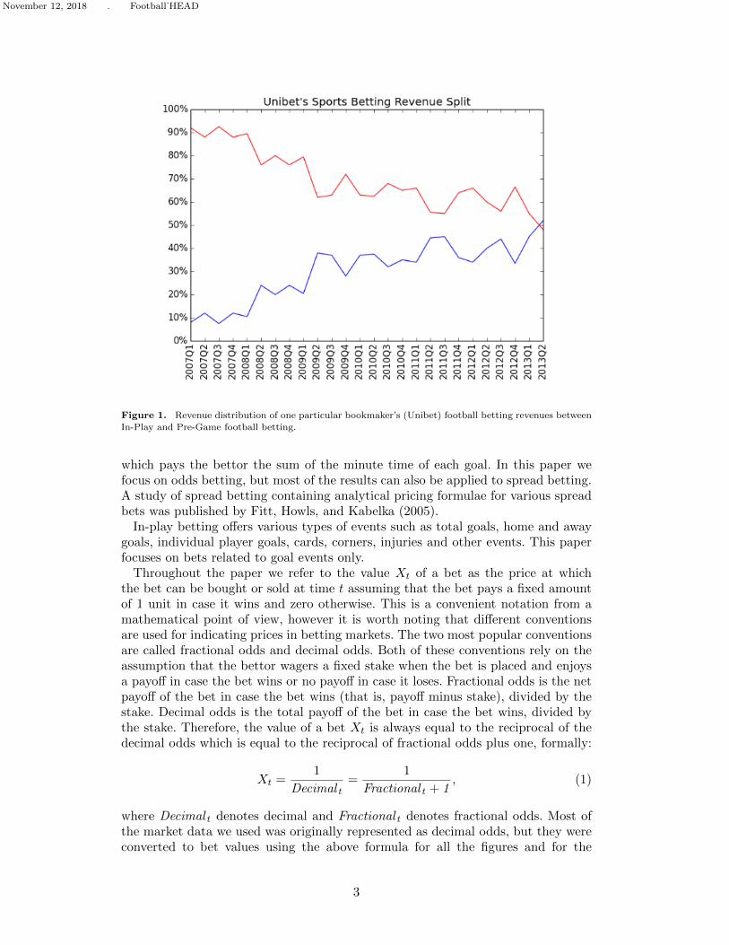
In traditional football betting, also known as pre-game or fixed odds betting, betsare placed before the beginning of the game. In-play football betting enables bettorsto place bets on the outcome of a game after it started. The main difference isthat during in-play betting, as the game progresses and as the teams score goals,the chances of certain outcomes jump to new levels and so do the odds of thebets. Prices move smoothly between goals and jump once a goal is scored. In-play betting became increasingly popular in recent years. For instance, Compliance(2013) recently reported that for one particular bookmaker (Unibet) in-play bettingrevenues exceeded pre-game betting revenues by 2013Q2 as shown in Figure 1.

There are two main styles of in-play betting: odds betting and spread betting.In odds betting, the events offered are similar to digital options in the sense thatthe bettor wins a certain amount if the event happens and loses a certain amountotherwise. Typical odds bets are whether one team wins the game, whether the totalnumber of goals is above a certain number or whether the next goal is scored bythe home team. In spread betting, the bets offered are such that the bettor can winor lose an arbitrary amount. A typical example is a bet called “total goal minutes”

2


Figure 1. Revenue distribution of one particular bookmaker’s (Unibet) football betting revenues betweenIn-Play and Pre-Game football betting.

which pays the bettor the sum of the minute time of each goal. In this paper wefocus on odds betting, but most of the results can also be applied to spread betting.A study of spread betting containing analytical pricing formulae for various spreadbets was published by Fitt, Howls, and Kabelka (2005).

In-play betting offers various types of events such as total goals, home and awaygoals, individual player goals, cards, corners, injuries and other events. This paperfocuses on bets related to goal events only.

Throughout the paper we refer to the value Xt of a bet as the price at whichthe bet can be bought or sold at time t assuming that the bet pays a fixed amountof 1 unit in case it wins and zero otherwise. This is a convenient notation from amathematical point of view, however it is worth noting that different conventionsare used for indicating prices in betting markets. The two most popular conventionsare called fractional odds and decimal odds. Both of these conventions rely on theassumption that the bettor wagers a fixed stake when the bet is placed and enjoysa payoff in case the bet wins or no payoff in case it loses. Fractional odds is the netpayoff of the bet in case the bet wins (that is, payoff minus stake), divided by thestake. Decimal odds is the total payoff of the bet in case the bet wins, divided bythe stake. Therefore, the value of a bet Xt is always equal to the reciprocal of thedecimal odds which is equal to the reciprocal of fractional odds plus one, formally:

Xt =1

Decimal t=

1

Fractional t + 1, (1)

where Decimal t denotes decimal and Fractional t denotes fractional odds. Most ofthe market data we used was originally represented as decimal odds, but they wereconverted to bet values using the above formula for all the figures and for the

3


underlying calculations in this paper.It is also worth noting that bets can be bought or sold freely during the game.

This includes going short which is referred to as lay betting. Mathematically thismeans that the amount held can be a negative number.

In-play bets can be purchased from retail bookmakers at a price offered by thebookmaker, but can also be traded on centralized marketplaces where the exchangemerely matches orders of participants trading with each other through a limit orderbook and keeps a deposit from each party to cover potential losses.

2.1 An example game

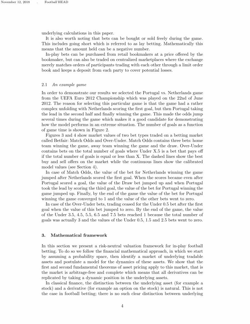
In order to demonstrate our results we selected the Portugal vs. Netherlands gamefrom the UEFA Euro 2012 Championship which was played on the 22nd of June2012. The reason for selecting this particular game is that the game had a rathercomplex unfolding with Netherlands scoring the first goal, but then Portugal takingthe lead in the second half and finally winning the game. This made the odds jumpseveral times during the game which makes it a good candidate for demonstratinghow the model performs in an extreme situation. The number of goals as a functionof game time is shown in Figure 2.

Figures 3 and 4 show market values of two bet types traded on a betting marketcalled Betfair: Match Odds and Over-Under. Match Odds contains three bets: hometeam winning the game, away team winning the game and the draw. Over-Undercontains bets on the total number of goals where Under X.5 is a bet that pays offif the total number of goals is equal or less than X. The dashed lines show the bestbuy and sell offers on the market while the continuous lines show the calibratedmodel values (see Section 4).

In case of Match Odds, the value of the bet for Netherlands winning the gamejumped after Netherlands scored the first goal. When the scores became even afterPortugal scored a goal, the value of the Draw bet jumped up and when Portugaltook the lead by scoring the third goal, the value of the bet for Portugal winning thegame jumped up. Finally, by the end of the game the value of the bet for Portugalwinning the game converged to 1 and the value of the other bets went to zero.

In case of the Over-Under bets, trading ceased for the Under 0.5 bet after the firstgoal when the value of this bet jumped to zero. By the end of the game, the valueof the Under 3.5, 4.5, 5.5, 6.5 and 7.5 bets reached 1 because the total number ofgoals was actually 3 and the values of the Under 0.5, 1.5 and 2.5 bets went to zero.

3. Mathematical framework

In this section we present a risk-neutral valuation framework for in-play footballbetting. To do so we follow the financial mathematical approach, in which we startby assuming a probability space, then identify a market of underlying tradableassets and postulate a model for the dynamics of these assets. We show that thefirst and second fundamental theorems of asset pricing apply to this market, that isthe market is arbitrage-free and complete which means that all derivatives can bereplicated by taking a dynamic position in the underlying assets.

In classical finance, the distinction between the underlying asset (for example astock) and a derivative (for example an option on the stock) is natural. This is notthe case in football betting; there is no such clear distinction between underlying

4


Figure 2. Scores of the two teams during the Portugal vs. Netherlands game on the 22nd of June, 2012.

The half time result was 1-1 and the final result was a 2-1 win for Portugal.

and derivative assets because all bets are made on the scores, and the score processitself is not a tradable asset. In order to be able to apply the Fundamental Theoremsof Asset Pricing we need to artificially introduce underlying assets and define themodel by postulating a price dynamics for these assets in the physical measure. It isalso desirable to chose underlying assets that have a simple enough price dynamicsso that developing the replicating portfolio becomes as straightforward as possible.For these reasons, the two underlying assets of our choice are assets that at theend of the game pay out the number of goals scored by the home and away teams,respectively. It is important to note that these assets are not traded in practiceand the choice therefore seems unnatural. However, these underlying assets can bestatically replicated from Arrow-Debreu securities that are referred to as CorrectScore bets in football betting and are traded in practice. Furthermore, towards theend of the Section 3.2 we arrive at Proposition 3.12 which states that any twolinearly independent bets can be used as hedging instruments. Therefore the choiceof the underlying assets is practically irrelevant and only serves a technical purpose.This result is applied in Section 5 where Next Goal bets are used as natural hedginginstruments.

3.1 Setup

Let us consider a probability space (Ω,F ,P) that carries two independent Poissonprocesses N1

t , N2t with respective intensities µ1, µ2 and the filtration (Ft)t∈[0,T ]

generated by these processes. Let time t = 0 denote the beginning and t = T theend of the game. The Poisson processes represent the number of goals scored by

5


Figure 3. Values of the three Match Odds bets during the game: Draw (black), Portugal Win (red),Netherlands Win (blue). Dashed lines represent the best market buy and sell offers while the continuous

lines represent the calibrated model values. Note that the value of the Netherlands Win bet jumps up afterthe first goal because the chance for Netherlands winning the game suddenly increased. It jumped down for

similar reasons when Portugal scored it’s first goal and at the same time the value of the Portugal Win and

Draw bets jumped up. By the end of the game, because Portugal actually won the game, the value of thePortugal Win bet reached 1 while both other bets became worthless.

the teams, the superscript 1 refers to the home and 2 refers to the away team. Thisnotation is used throughout, the distinction between superscripts and exponentswill always be clear from the context. The probability measure P is the real-worldor physical probability measure.

We assume that there exists a liquid market where three assets can be tradedcontinuously with no transaction costs or any restrictions on short selling or bor-rowing. The first asset Bt is a risk-free bond that bears no interests, an assumptionthat is motivated by the relatively short time frame of a football game. The secondand third assets S1

t and S2t are such that their values at the end of the game are

equal to the number of goals scored by the home and away teams, respectively.

Definition 3.1 (model). The model is defined by the following price dynamics ofthe assets:

Bt = 1

S1t = N1

t + λ1 (T − t) (2)

S2t = N2

t + λ2 (T − t)

where λ1 and λ2 are known real constants.

Essentially, the underlying asset prices are compensated Poisson processes, but the

6


Figure 4. Values of Over/Under bets during the game. Under X.5 is a bet that pays off in case the totalnumber of goals by the end of the game is below or equal to X. Marked lines represent the calibrated model

prices while the grey bands show the best market buy and sell offers. Note that after the first goal tradingin the Under 0.5 bet ceased and it became worthless. By the end of the game when the total number of

goals was 3, all the bets up until Under 2.5 became worthless while the Under 3.5 and higher bets reached

a value of 1.

compensators λ1, λ2 are not necessarily equal to the intensities µ1, µ2 and thereforethe prices are not necessarilty martingales in the physical measure P. This is similarto the Black-Scholes model where the stock’s drift in the physical measure is notnecessarily equal to the risk-free rate.

We are now closely following Harrison and Pliska (1981) in defining the necessaryconcepts.

3.2 Risk-neutral pricing of bets

Definition 3.2 (trading strategy). A trading strategy is an Ft-predictable vec-

tor process φt =(φ0t , φ

1t , φ

2t

)that satisfies

∫ t0

∣∣φis∣∣ ds < ∞ for i ∈ 0, 1, 2. Theassociated value process is denoted by

V φt = φ0

tBt + φ1tS

1t + φ2

tS2t . (3)

The trading strategy is self-financing if

V φt = V φ

0 +

∫ t

0φ1sdS

1s +

∫ t

0φ2sdS

2s . (4)

where∫ t

0 φisdS

is, i ∈ 1, 2 is a Lebesgue Stieltjes integral which is well defined

according to Proposition 2.3.2 on p17 of Bremaud (1981).

7


Definition 3.3 (arbitrage-freeness). The model is arbitrage-free if no self-

financing trading strategy φt exist such that P[V φt − V

φ0 ≥ 0

]= 1 and

P[V φt − V

φ0 > 0

]> 0.

Definition 3.4 (bet). A bet (also referred to as a contingent claim or derivative)is an FT -measurable random variable XT .

In practical terms this means that the value of a bet is revealed at the end of thegame.

Definition 3.5 (completeness). The model is complete if for every bet XT there

exists a self-financing trading strategy φt such that XT = V φT . In this case we say

that the bet XT is replicated by the trading strategy φt.

Theorem 3.6 (risk-neutral measure). There exists a probability measure Q re-ferred to as the risk-neutral equivalent martingale measure such that:

(a) The asset processes Bt, S1t , S2

t are Q-martingales.(b) The goal processes N1

t and N2t in measure Q are standard Poisson processes

with intensities λ1 and λ2 respectively (which are in general different from theP-intensities of µ1 and µ2).

(c) Q is an equivalent measure to P, that is the set of events having zero probabilityis the same for both measures.

(d) Q is unique.

Proof. The proof relies on Girsanov’s theorem for point processes (see Theorem 2on p.165 and Theorem 3 on page 166 in Bremaud (1981)) which states that N1

t andN2t are Poisson processes with intensities λ1 and λ2 under the probability measure

Q which is defined by the Radon-Nikodym-derivative

dQdP

= Lt, (5)

where

Lt =

2∏i=1

(λiµi

)N it

exp [(µi − λi) t] . (6)

Then uniqueness follows from Theorem 8 on p.64 in Bremaud (1981) which statesthat if two measures have the same set of intensities, then the two measures mustcoincide. The Integration Theorem on p.27 of Bremaud (1981) states that N i

t − λitare Q-martingales, therefore the assets Sit are also Q-martingales for i ∈ 1, 2.Proposition 9.5 of Tankov (2004) claims that P and Q are equivalent probabilitymeasures. The process of the bond asset Bt is a trivial martingale in every measurebecause it’s a deterministic constant which therefore doesn’t depend on the measure.

Remark 3.7. Changing the measure of a Poisson process changes the intensity andleaves the drift unchanged. This is in contrast with the case of a Wiener processwhere change of measure changes the drift and leaves the volatility unchanged.

8


Theorem 3.8. (arbitrage-free) The model is arbitrage-free and complete.

Proof. This follows directly from the first and second fundamental theorems of fi-nance. To be more specific, arbitrage-freeness follows from theorem 1.1 of Delbaenand Schachermayer (1994) which states that the existence of a risk-neutral mea-sure implies a so-called condition “no free lunch with vanishing risk” which impliesarbitrage-freeness. Completeness follows from theorem 3.36 of Harrison and Pliska(1981) which states that the model is complete if the risk-neutral measure is unique.Alternatively it also follows from theorem 3.35 which states that the model is com-plete if the martingale representation theorem holds for all martingales which is thecase according to Theorem 17, p.76 of Bremaud (1981).

Corollary 3.9. The time-t value of a bet is equal to the risk-neutral expectationof it’s value at the end of the game, formally:

Xt = EQ [XT |Ft] . (7)

Proof. This follows directly from Proposition 3.31 of Harrison and Pliska (1981).

Corollary 3.10. The time-t value of a bet is also equal to the value of the associ-ated self-financing trading strategy φt, formally:

Xt = V φt = V φ

0 +

∫ t

0φ1sdS

1s +

∫ t

0φ2sdS

2s . (8)

Proof. This follows directly from Proposition 3.32 of Harrison and Pliska (1981).

Definition 3.11 (linear independence). The bets Z1T and Z2

T are linearly in-dependent if the self-financing trading strategy φ1

t =(φ10t , φ

11t , φ

12t

)that replicates

Z1T is P-almost surely linearly independent from the self-financing trading strategy

φ2t =

(φ20t , φ

21t , φ

22t

)that replicates Z2

T . Formally, at any time t ∈ [0, T ] and for anyconstants c1, c2 ∈ R

c1φ1t 6= c2φ

2t P a.s. (9)

Proposition 3.12 (replication). Any bet XT can be replicated by taking a dynamicposition in any two linearly independent bets Z1

T and Z2T , formally:

Xt = X0 +

∫ t

0ψ1sdZ

1s +

∫ t

0ψ2sdZ

2s , (10)

where the weights ψ1t , ψ

2t are equal to the solution of the following equation:(

φ11t φ12

t

φ21t φ22

t

)(ψ1t

ψ2t

)=

(φ1t

φ2t

)(11)

where(φ11t , φ

12t

),(φ21t , φ

22t

)and

(φ1t , φ

2t

)are the components of the trading strat-

egy that replicates Z1T , Z2

T and XT , respectively. The integral∫ t

0 ψ1sdZ

1s is to be

9


interpreted in the following sense:∫ t

0ψ1sdZ

1s =

∫ t

0ψ1sφ

11s dS

1s +

∫ t

0ψ1sφ

12s dS

2s (12)

and similarly for∫ t

0 ψ2sdZ

2s .

Proof. Substituting dZ1t = φ11

t dS1t + φ21

t dS2t , dZ2

t = φ12t dS

1t + φ22

t dS2t and Equation

8 into Equation 10 verifies the proposition.

3.3 European bets

Definition 3.13 (European bet). A European bet is a bet with a value dependingonly on the final number of goals N1

T , N2T , that is one of the form

XT = Π(N1T , N

2T

)(13)

where Π is a known scalar function N × N → R which is referred to as the payofffunction.

Example 3.14. A typical example is a bet that pays out 1 if the home teamscores more goals than the away team (home wins) and pays nothing otherwise,that is Π

(N1T , N

2T

)= 1

(N1T > N2

T

)where the function 1 (A) takes the value of 1

if A is true and zero otherwise. Another example is a bet that pays out 1 if thetotal number of goals is strictly higher than 2 and pays nothing otherwise, that isΠ(N1T , N

2T

)= 1

(N1T +N2

T > 2).

Proposition 3.15 (pricing formula). The time-t value of a European bet withpayoff function Π is given by the explicit formula

Xt =

∞∑n1=N t

1

∞∑n2=N t

2

Π (n1, n2)P(n1 −N1

t , λ1 (T − t))P(n2 −N2

t , λ2 (T − t)), (14)

where P (N,Λ) is the Poisson probability, that is P (N,Λ) = e−Λ

N ! ΛN if N ≥ 0 andP (N,Λ) = 0 otherwise.

Proof. This follows directly form Proposition 3.9 and Definition 3.13.

As we have seen, the price of a European bet is a function of the time t and thenumber of goals

(N1t , N

2t

)and intensities (λ1, λ2). Therefore, from now on we will

denote this function by Xt = Xt

(N1t , N

2t

)or Xt = Xt

(t,N1

t , N2t , λ1, λ2

), depending

on whether the context requires the explicit dependence on intensities or not.It is important to note that Arrow-Debreu bets do exist in in-play football betting

and are referred to as Correct Score bets.

Definition 3.16 (Arrow-Debreu bets). Arrow-Debreu bets, also known as Cor-rect Score bets are European bets with a payoff function ΠAD(K1,K2) equal to 1 if

the final score(N1T , N

2T

)is equal to a specified result (K1,K2) and 0 otherwise:

ΠAD(K1,K2) = 1(N1T = K1, N

2T = K2

)(15)

10


According to the following proposition, Arrow-Debreu bets can be used to stati-cally replicate any European bet:

Proposition 3.17 (static replication). The time-t value of a European bet withpayoff function Π in terms of time-t values of Arrow-Debreu bets is given by:

Xt =

∞∑K1=N t

1

∞∑K2=N t

2

Π (K1,K2)Xt,AD(K1,K2), (16)

where Xt,AD(K1,K2) denotes the time-t value of an Arrow-Debreu bet that pays outif the final scores are equal to (K1,K2).

Proof. This follows directly form Proposition 3.15 and Definition 3.16.

Let us now define the partial derivatives of the bet values with respect to changein time and the number goals scored. These are required for hedging and serve thesame purpose as the greeks in the Black-Scholes framework.

Definition 3.18 (Greeks). The greeks are the values of the following forward dif-ference operators (δ1, δ2) and partial derivative operator applied to the bet value:

δ1Xt

(N1t , N

2t

)= Xt

(N1t + 1, N2

t

)−Xt

(N1t , N

2t

)(17)

δ2Xt

(N1t , N

2t

)= Xt

(N1t , N

2t + 1

)−Xt

(N1t , N

2t

)(18)

∂tXt

(N1t , N

2t

)= lim

dt→0

1

dt

[Xt+dt

(N1t , N

2t

)−Xt

(N1t , N

2t

)](19)

Remark. The forward difference operators δ1, δ2 play the role of Delta and thepartial derivative operator ∂t plays the role of Theta in the Black-Scholes framework.

Theorem 3.19 (Kolmogorov forward equation). The value of a European betX(t,N1

t , N2t

)with a payoff function Π(N1

T , N2T ) satisfies the following Feynman-Kac

representation on the time interval t ∈ [0, T ] which is also known as the Kolmogorovforward equation:

∂tX(t,N1

t , N2t

)= −λ1δ1X

(t,N1

t , N2t

)− λ2δ2X

(t,N1

t , N2t

)(20)

with boundary condition:

XT

(T,N1

T , N2T

)= Π

(N1T , N

2T

).

Proof. The proposition can be easily verified using the closed form formula fromProposition 3.15. Furthermore, several proofs are available in the literature, see forexample Proposition 12.6 in Tankov (2004), Theorem 6.2 in Ross (2006) or Equation13 in Feller (1940).

Remark 3.20. Equation 20 also has the consequence that any portfolio of Euro-pean bets that changes no value if either team scores a goal (Delta-neutral) doesnot change value between goals either (Theta-neutral). We note without a proof,that this holds for all bets in general.

11


Corollary 3.21. The value of a European bet X(t,N1

t , N2t , λ1, λ2

)satisfies the

following:

∂

∂λiXt = (T − t) δiXt (21)

where i ∈ 1, 2.

Proof. This follows directly from Proposition 3.15.

Proposition 3.22 (portfolio weights). The components(φ1t , φ

2t

)of the trading

strategy that replicates a European bet XT are equal to the forward differenceoperators (δ1, δ2) of the bet, formally:

φ1t = δ1X

(t,N1

t , N2t

)(22)

φ2t = δ2X

(t,N1

t , N2t

). (23)

Proof. Recall that according to Proposition 3.10, the time-t value of a bet is equalto Xt = X0 +

∑2i=1

∫ t0 φ

isdS

is, which after substituting dSit = dN i

t − λidt becomes

Xt = X0 +

∫ t

0

(φ1sλ1 + φ2

sλ2

)ds

+

N1t∑

k=0

φ1t1k

+

N2t∑

k=0

φ2t2k, (24)

where we used∫ t

0 φisdN

is =

∑N it

k=0 φit1k

where 0 ≤ tik ≤ t is the time of the k.th jump

(goal) of the process N it for i ∈ 1, 2.

On the other hand, using Ito’s formula for jump processes (Proposition 8.15,Tankov (2004)), which applies because the closed form formula in Proposition 3.15is infinitely differentiable, the value of a European bet is equal to

Xt = X0 +

∫ t

0∂sX

(s,N1

s , N2s

)ds

+

N1t∑

k=0

δ1X(t1k, N

1t1k−, N

2t1k−

)+

N2t∑

k=0

δ2X(t2k, N

1t2k−, N

2t2k−

), (25)

where tik− refers to the fact that the value of the processes is to be taken before thejump.

Because the equality between Equations 24 and 25 hold for every possible jumptimes, the terms behind the sums are equal which proves the proposition.

4. Model Calibration

In this section we discuss how to calibrate the model parameters to historical marketprices. We demonstrate that a unique equivalent martingale measure Q exists, thatis, a set of intensities λ1, λ2 exist that are consistent with the prices of all betsobserved on the market (see Propositions 3.6 and 3.8).

12


We apply a least squares approach in which we consider market prices of a setof bets and find model intensities that deliver model prices for these bets that areas close as possible to the market prices. Specifically, we minimize the sum of thesquare of the weighted differences between the model and market mid prices as afunction of model intensities, using market bid-ask spreads as weights. The reasonfor choosing a bid-ask spread weighting is that we would like to take into accountbets with a lower bid-ask spread with a higher weight because the price of thesebets is assumed to be more certain. Formally, we minimize the following expression:

R(λ1t , λ

2t

)=

√√√√√ 1

n

n∑i=1

Xi,MIDt −Xi

t

(λ1t , λ

2t , N

1t , N

2t

)12

(Xi,SELLt −Xi,BUY

t

)2

, (26)

where n is the total number of bets used, Xi,BUYt and Xi,SELL

t are the best market

buy and sell quotes of the i.th type of bet at time t, Xi,MIDt is the market mid price

which is the average of the best buy and sell quotes, Xit

(N1t , N

2t , λ

1t , λ

2t

)is the model

price of the i.th bet at time t, given the current number of goals N1t , N

2t and model

intensity parameters λ1t , λ

2t , see Proposition 3.15. This minimization procedure is

referred to as model calibration.Calibration has been performed using a time step of 1 minute during the game,

independently at each time step. We used the three most liquid groups of bets whichin our case were Match Odds, Over / Under and Correct Score with a total of 31bet types in these three categories. Appendix A describes these bet types in detail.

The continuous lines in Figures 3 and 4 show the calibrated model prices whilethe dashed lines are the market buy and sell offers. It can be seen that the calibratedvalues are close to the market quotes, although they are not always within the bid-ask spread. As the measures of the goodness of the fit we use the optimal value ofthe cost function of Equation 26, which is the average distance of the calibratedvalues from the market mid prices in units of bid-ask spread, the calibration erroris shown in Figure 5. We performed calibration for multiple games of the Euro 2012Championship, the time average of the calibration errors for each game is shown inTable 1. The mean and standard deviation of the calibration errors across gamesis 1.57 ± 0.27 which is to be interpreted in units of bid-ask spread because of theweighting of the error function in Equation 26. This means, that on average, thecalibrated values are outside of the bid-ask spread, but not significantly. Given thata model of only 2 parameters has been calibrated to a total of 31 independentmarket quotes, this is a reasonably good result.

Finally, the implied intensities, along with the estimated uncertainties of the cal-ibration using the bid-ask spreads are shown in Figure 6. Contrary to our initialassumption of constant intensities, the actual intensities fluctuate over time andthere also seems to be an increasing trend in the implied goal intensities of bothteams.

In order to better understand the nature of the implied intensity process, weestimated the drift and volatility of the log total intensity, that is we assumed thefollowing:

d ln(λ1t + λ2

t

)= µdt+ σdWt (27)

13


Figure 5. Calibration error during the game. Calibration error is defined as the average distance of all

31 calibrated bet values from the market mid prices in units of bid-ask spread. A formal definition is given

by Equation 26. Note that the calibration error for this particular game is usually between 1 and 2 bid-askspreads which is a reasonably good result, given that the model has only 2 free parameters to explain all

31 bet values.

where µ and σ are the drift and volatility of the process. Table 2 shows the resultsof the estimation for multiple games. The mean and standard deviation of the driftterms are µ = 0.55 ± 0.16 1/90min while the mean and standard deviation of thevolatility terms are σ = 0.51±0.19 1/

√90min. The fact that implied goal intensities

are increasing during the game is consistent with findings of Dixon and Robinson(1998) who found gradual increase of scoring rates by analysing goal times of 4012matches between 1993 and 1996.

5. Hedging with Next Goal bets

In this section we demonstrate market completeness and we show that Next Goalbets are natural hedging instruments that can be used to dynamically replicate andhedge other bets.

Recall that according to Proposition 3.12 any European bet Xt can be replicatedby dynamically trading in two linearly independent instruments Z1

t and Z2t :

Xt = X0 +

∫ t

0ψ1sdZ

1s +

∫ t

0ψ2sdZ

2s (28)

14


Figure 6. Calibrated model parameters, also referred to as implied intensities during the game. Formally,

this is equal to the minimizer λ1t , λ

2t of Equation 26. The bands show the parameter uncertainties estimated

from the bid-ask spreads of the market values of the bets. Note that the intensities appear to have an

increasing trend and also fluctuate over time.

Game Calibration ErrorDenmark v Germany 1.65Portugal v Netherlands 1.18Spain v Italy 2.21Sweden v England 1.58Italy v Croatia 1.45Germany v Italy 1.50Germany v Greece 1.34Netherlands v Germany 1.78Spain v Rep of Ireland 1.64Spain v France 1.40

Average 1.57Standard deviation 0.27

Table 1. Average calibration errors in units of bid-ask spread as shown in Figure 5 have been calculatedfor multiple games of the UEFA Euro 2012 Championship and are shown in this table. Note that the mean

of the averages is just 1.57 bid-ask spreads with a standard deviation of 0.27 which shows that the modelfit is reasonably good for the games analysed.

where the portfolio weights ψ1t , ψ

2t are equal to the solution of the equation(

δ1Z1t δ1Z

2t

δ2Z1t δ2Z

2t

)(ψ1t

ψ2t

)=

(δ1Xt

δ2Xt

), (29)

where the values of the finite difference operators δ (Definition 3.18) can be com-

15


Game Drift [1/90min] Vol [1/√

90min]Denmark v Germany 0.36 0.28Portugal v Netherlands 0.49 0.44Spain v Italy 0.60 0.76Sweden v England 0.58 0.59Italy v Croatia 0.82 0.60Germany v Italy 0.76 0.39Germany v Greece 0.65 0.66Netherlands v Germany 0.43 0.32Spain v Rep of Ireland 0.32 0.78Spain v France 0.48 0.25

Average 0.55 0.51Standard deviation 0.16 0.19

Table 2. Average drift and volatility of total log-intensities estimated for multiple games of the UEFA

Euro 2012 Championship. Note that the drift term is positive for all games which is consistent with theempirical observation of increasing goal frequencies as the game progresses.

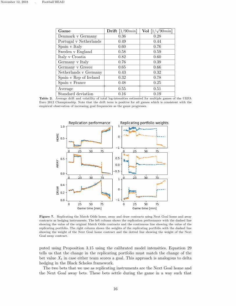
Figure 7. Replicating the Match Odds home, away and draw contracts using Next Goal home and awaycontracts as hedging instruments. The left column shows the replication performance with the dashed lineshowing the value of the original Match Odds contracts and the continuous line showing the value of the

replicating portfolio. The right column shows the weights of the replicating portfolio with the dashed lineshowing the weight of the Next Goal home contract and the dotted line showing the weight of the Next

Goal away contract.

puted using Proposition 3.15 using the calibrated model intensities. Equation 29tells us that the change in the replicating portfolio must match the change of thebet value Xt in case either team scores a goal. This approach is analogous to deltahedging in the Black Scholes framework.

The two bets that we use as replicating instruments are the Next Goal home andthe Next Goal away bets. These bets settle during the game in a way such that

16


when the home team scores a goal the price of the Next Goal home bet jumps to 1and the price of the Next Goal away bet jumps to zero and vice versa for the awayteam. After the goal the bets reset and trade again at their regular market price.The values of the bets are:

ZNG1

t =λ1

λ1 + λ2

[1− e−(λ1+λ2)(T−t)

](30)

ZNG2

t =λ2

λ1 + λ2

[1− e−(λ1+λ2)(T−t)

]. (31)

The matrix of deltas, that is the changes of contract values in case of a goal asdefined in 3.18 are:

(δ1Z

NG1

t δ1ZNG2

t

δ2ZNG1

t δ2ZNG2

t

)=

(1− ZNG1

t −ZNG2

t

−ZNG1

t 1− ZNG2

t

)(32)

The reason for choosing Next Goal bets as hedging instruments is that thesebets are linearly independent (see Definition 3.11), that is the delta matrix is non-singular even if there is a large goal difference between the two teams. Note that thisis an advantage compared to using the Match Odds bets as hedging instruments: incase one team leads by several goals, it is almost certain that the team will win. Inthat case the value of the Match Odds bets goes close to 1 for the given team and0 for the other team. An additional goal does not change the values significantly,therefore the delta matrix becomes singular and the bets are not suitable for hedgingbecause the portfolio weights go to infinity. This is never the case with Next Goalbets which can therefore be used as natural hedging instruments.

We used the Portugal vs. Netherlands game from Section 2.1 to replicate the valuesof the three Match Odds bets, using the Next Goal bets as hedging instruments.Figure 7 shows the values of the original Match Odds bets along with the values ofthe replicating portfolios (left column) and the replicating portfolio weights (rightcolumn).

Figure 8 shows the jumps of contract values against the jumps of replicating port-folio values at times when a goal was scored. This figure contains several differenttypes of bets, that is not only Match Odds bets, but also Over/Under and Cor-rect Score bets. The figure also contains all 3 goals scored during the Portugal vs.Netherlands game. It can be seen that the jumps of the original contract valuesare in line with the jumps of the replicating portfolio values with a correlation of89%. Table 3 shows these correlations for multiple games of the UEFA Euro 2012Championship. It can be seen that the correlations are reasonably high for all gameswith an average of 80% and a standard deviation of 19%.

6. Conclusions

In this paper we have shown that the Fundamental Theorems of Asset Pricing applyto the market of in-play football bets if the scores are assumed to follow independentPoisson processes of constant intensities. We developed general formulae for pricingand replication. We have shown that the model of only 2 parameters calibrates

17


Figure 8. Jumps of actual contract values (horizontal axis) versus jumps of replicating portfolio values(vertical axis) at times of goals scored during the Portugal vs. Netherlands game. The changes are computed

between the last traded price before a goal and the first traded price after a goal, for all goals. The figure

contains Match Odds, Over/Under and Correct Score bets. Next Goal home and away bets were usedas hedging instruments to build the replicating portfolios. Note that the value changes of the replicating

portfolios corresponds reasonably well to the value changes of the original contracts with a correlation of

89%.

Game CorrelationDenmark vs. Germany 79%Portugal vs. Netherlands 89%Spain vs. Italy 97%Italy vs. Croatia 47%Spain vs. France 86%Germany vs. Italy 99%Germany vs. Greece 60%Netherlands vs. Germany 93%Spain vs. Rep of Ireland 98%Sweden vs. England 50%

Average 80%Standard deviation 19%

Table 3. Correlation between the jumps of bet values and jumps of replicating portfolios at times of goalsfor all bets of a game.

to 31 different bets with an error of less than 2 bid-ask spreads. Furthermore, wehave shown that the model can also be used for replication and hedging. Overallwe obtained good agreement between actual contract values and the values of thecorresponding replicating portfolios, however we point out that hedging errors cansometimes be significant due to the fact the implied intensities are in practice notconstant.

18


Funding

PD and TA acknowledge support of the Economic and Social Research Council(ESRC) in funding the Systemic Risk Centre (ES/K002309/1).

References

Back, Kerry, and Stanley R Pliska. 1991. “On the fundamental theorem of asset pricing with aninfinite state space.” Journal of Mathematical Economics 20 (1): 1–18.

Bremaud, Pierre. 1981. Point processes and queues. Vol. 30. Springer, New York.Compliance, Gambling. 2013. “In-Play Tracker - Summer 2013.” .Cox, John C, and Stephen A Ross. 1976. “The valuation of options for alternative stochastic

processes.” Journal of Financial Economics 3 (1): 145–166.Delbaen, Freddy, and Walter Schachermayer. 1994. “A general version of the fundamental theorem

of asset pricing.” Mathematische annalen 300 (1): 463–520.Dixon, Mark, and Michael Robinson. 1998. “A birth process model for association football

matches.” Journal of the Royal Statistical Society: Series D (The Statistician) 47 (3): 523–538.Dixon, Mark J, and Stuart G Coles. 1997. “Modelling association football scores and inefficien-

cies in the football betting market.” Journal of the Royal Statistical Society: Series C (AppliedStatistics) 46 (2): 265–280.

Duffie, Darrell. 1988. Security markets: Stochastic models. Vol. 19821. Academic Press New York.Feller, Willy. 1940. “On the integro-differential equations of purely discontinuous Markoff pro-

cesses.” Transactions of the American Mathematical Society 48 (3): 488–515.Fitt, AD, CJ Howls, and M Kabelka. 2005. “Valuation of soccer spread bets.” Journal of the

Operational Research Society 57 (8): 975–985.Harrison, J Michael, and David M Kreps. 1979. “Martingales and arbitrage in multiperiod securities

markets.” Journal of Economic Theory 20 (3): 381–408.Harrison, J Michael, and Stanley R Pliska. 1981. “Martingales and stochastic integrals in the theory

of continuous trading.” Stochastic processes and their applications 11 (3): 215–260.Harrison, J Michael, and Stanley R Pliska. 1983. “A stochastic calculus model of continuous trading:

complete markets.” Stochastic processes and their applications 15 (3): 313–316.Huang, Chi-Fu. 1985. “Information structure and equilibrium asset prices.” Journal of Economic

Theory 35 (1): 33–71.Jottreau, Benoit. 2009. “How do markets play soccer?.” .Maher, MJ. 1982. “Modelling association football scores.” Statistica Neerlandica 36 (3): 109–118.Ross, Sheldon M. 2006. Introduction to probability models. Academic press, Massachusetts.Tankov, Peter. 2004. Financial modelling with jump processes. CRC Press, London.Vecer, Jan, Frantisek Kopriva, and Tomoyuki Ichiba. 2009. “Estimating the effect of the red card

in soccer: When to commit an offense in exchange for preventing a goal opportunity.” Journalof Quantitative Analysis in Sports 5 (1).

Appendix A. Valuation formulae

This section summarizes a list of analytical formulae for the values of some of themost common in-play football bets. In the first sub-section we consider Europeanbets, while the second sub-section contains non-European bets.

A.1 European Bets

The value of a European bet at the end of the game only depends on the finalscores. The formulae of this section follow directly from Proposition 3.15. Table A1summarizes the payoff functions and the valuation formulae for some of the most

19


Bet type Payoff Π(N1T , N

2T

)Value Xt

(N1t , N

2t , λ1, λ2

)Match Odds Home 1

(N1T > N2

T

) ∑k1>k2

∏2i=1 P

(ki −N i

t ,Λi)

Match Odds Away 1(N1T < N2

T

) ∑k1<k2

∏2i=1 P

(ki −N i

t ,Λi)

Match Odds Draw 1(N1T = N2

T

) ∑k1=k2

∏2i=1 P

(ki −N i

t ,Λi)

Arrow-Debreu K1,K2 1(N1T = K1, N

2T = K2

) ∏2i=1 P

(Ki −N i

t ,Λi)

Over K 1(N1T +N2

T > K) ∑∞

k=K+1 P(k −N1

t −N2t , (Λ1 + Λ2)

)Under K 1

(N1T +N2

T < K) ∑K−1

k=0 P(k −N1

t −N2t , (Λ1 + Λ2)

)Odd 1

(N1T +N2

T = 1 mod 2)

exp [− (Λ1 + Λ2)] cosh [(Λ1 + Λ2)]Even 1

(N1T +N2

T = 0 mod 2)

exp [− (Λ1 + Λ2)] sinh [(Λ1 + Λ2)]

Winning Margin K 1(N1T −N2

T = K) exp [− (Λ1 + Λ2)]

(Λ1

Λ2

)K−N1t +N2

t2

·B|K−N1t +N2

t |(2√

Λ1Λ2

)Table A1. Valuation formulae for some of the most common types of in-play football bets. Π

(N1

T , N2T

)denotes the payoff function, that is the value of the European bet at the end of the game. P (k,Λ) denotesthe Poisson distribution, that is P (k,Λ) = 1

k!e−ΛΛk and Λi = λi (T − t) with i ∈ 1, 2 for the home and

the away team, respectively.

common types of European bets.Match Odds Home, Away and Draw bets pay out depending on the final result

of the game. The Arrow-Debreu K1,K2 bets pay out if the final scores are equal toK1,K2. Over K and Under K bets pay out if the total number of goals is over orunder K. Odd and Even bets pay out if the total number of goals is an odd or aneven number.

The Winning Margin K bet wins if the difference between the home and awayscores is equal to K. The value of this bet follows the Skellam distribution, Bk (z)denotes the modified Bessel function of the first kind.

A.2 Non-European Bets

Bets in this category have a value at the end of the game that depends not onlyon the final score, but also on the score before the end of the game or the order ofscores. We consider two popular bets in this category: Next Goal and Half Time /Full Time bets. Valuation of these bets follows from Corollary 3.9.

A.2.1 Next Goal. The Next Goal Home bet wins if the home team scores the nextgoal. The value of this bet is

Xt =λ1

λ1 + λ2

[1− e−(λ1+λ2)(T−t)

]. (A1)

Similarly, the value of the Next Goal Away bet is equal to

Xt =λ2

λ1 + λ2

[1− e−(λ1+λ2)(T−t)

]. (A2)

A.2.2 Half Time / Full Time. Half Time / Full Time bets win if the half timeand the full time is won by the predicted team or is a draw. Given that there are 3

20


outcomes in each halves, there are 9 bets in this category. For example, the value ofthe Half Time Home / Full Time Draw bet before the end of the first half is equalto:

Xt =∑

k1>k2

∑l1=l2

P(k1 −N1

t , λ1

(T 1

2− t))

P(k2 −N2

t , λ2

(T 1

2− t))

×P(l1 − k1, λ1

(T − T 1

2

))P(l2 − k2, λ2

(T − T 1

2

)).(A3)

In the second half, this bet either becomes worthless if the first half was not wonby the home team or otherwise becomes equal to the Draw bet.

21

risk-neutral pricing and hedging of in-play football bets

Documents