risk-parity portfolio 10/slides_risk... · the expected return wtµ and the risk of the portfolio...

Risk-Parity Portfolio

Prof. Daniel P. PalomarThe Hong Kong University of Science and Technology (HKUST)

MAFS6010R- Portfolio Optimization with RMSc in Financial Mathematics

Fall 2018-19, HKUST, Hong Kong

Outline

1 Introduction

2 Warm-Up: Markowitz Portfolio

Signal modelMarkowitz formulationDrawbacks of Markowitz portfolio

3 Risk-Parity Portfolio

Problem formulationAlgorithms via SCA

4 Conclusions

Motivation

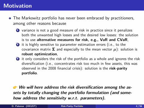
The Markowitz portfolio has never been embraced by practitioners,among other reasons because

1 variance is not a good measure of risk in practice since it penalizesboth the unwanted high losses and the desired low losses: the solutionis to use alternative measures for risk, e.g., VaR and CVaR,

2 it is highly sensitive to parameter estimation errors (i.e., to thecovariance matrix Σ and especially to the mean vector µ): solution isrobust optimization,

3 it only considers the risk of the portfolio as a whole and ignores the riskdiversification (i.e., concentrates risk too much in few assets, this wasobserved in the 2008 financial crisis): solution is the risk-parityportfolio.

We will here address the risk diversification among the as-sets by totally changing the portfolio formulation (and some-how address the sensitivity w.r.t. parameters).

D. Palomar (HKUST) Risk-Parity Portfolio 4 / 56

Outline

1 Introduction





4 Conclusions

Returns

Let us denote the log-returns of N assets at time t with the vectorrt ∈ RN.The time index t can denote any arbitrary period such as days, weeks,months, 5-min intervals, etc.Ft−1 denotes the previous historical data.Econometrics aims at modeling rt conditional on Ft−1.rt is a multivariate stochastic process with conditional mean andcovariance matrix denoted as1

µt ≜ E [rt | Ft−1]

Σt ≜ Cov [rt | Ft−1] = E[(rt − µt)(rt − µt)T | Ft−1

].

1Y. Feng and D. P. Palomar, A Signal Processing Perspective on FinancialEngineering. Foundations and Trends in Signal Processing, Now Publishers, 2016.


I.I.D. Model

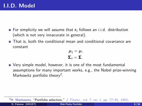
For simplicity we will assume that rt follows an i.i.d. distribution(which is not very innacurate in general).That is, both the conditional mean and conditional covariance areconstant

µt = µ,

Σt = Σ.

Very simple model, however, it is one of the most fundamentalassumptions for many important works, e.g., the Nobel prize-winningMarkowitz portfolio theory2.

2H. Markowitz, “Portfolio selection,” J. Financ., vol. 7, no. 1, pp. 77–91, 1952.D. Palomar (HKUST) Risk-Parity Portfolio 8 / 56

Parameter Estimation

Consider the i.i.d. model:

rt = µ + wt,

where µ ∈ RN is the mean and wt ∈ RN is an i.i.d. process with zeromean and constant covariance matrix Σ.The mean vector µ and covariance matrix Σ have to be estimated inpractice based on T observations.The simplest estimator is the sample estimator:

sample mean estimator: µ = 1T

∑Tt=1 rt

sample covariance matrix: Σ = 1T−1

∑Tt=1(rt − µ)(rt − µ)T.

Many more sophisticated estimators exist, namely: shrinkageestimators, Black-Litterman estimators, etc.


Parameter Estimation

The parameter estimates µ and Σ are only good for large T,otherwise the estimation error is unacceptable.For instance, the sample mean is particularly a very inefficientestimator, with very noisy estimates.3

In practice, T cannot be large enough due to either:unavailability of data orlack of stationarity of data.

As a consequence, the estimates contain too much estimation errorand a portfolio design (e.g., Markowitz mean-variance) based onthose estimates can be fatal.Indeed, this is why Markowitz portfolio and other extensions are rarelyused by practitioners.

3A. Meucci, Risk and Asset Allocation. Springer, 2005.D. Palomar (HKUST) Risk-Parity Portfolio 10 / 56

Outline

1 Introduction





4 Conclusions

Portfolio Return

Suppose the budget is B dollars.The portfolio w ∈ RN denotes the normalized weights of the assetssuch that 1Tw = 1 (then Bw denotes dollars invested in the assets).For each asset, the initial wealth is Bwi and the end wealth is

Bwi (pi,t/pi,t−1) = Bwi (Rit + 1) .

Then the portfolio return is

Rpt =

∑Ni=1 Bwi (Rit + 1)− B

B =N∑

i=1wiRit ≈

N∑i=1

wirit = wTrt

The portfolio expected return and variance are wTµ and wTΣw,respectively.4

4G. Cornuejols and R. Tütüncü, Optimization Methods in Finance. CambridgeUniversity Press, 2006.


Performance Measures

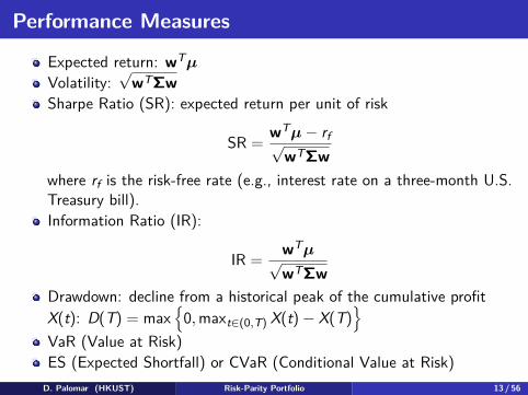
Expected return: wTµ

Volatility:√

wTΣwSharpe Ratio (SR): expected return per unit of risk

SR = wTµ− rf√wTΣw

where rf is the risk-free rate (e.g., interest rate on a three-month U.S.Treasury bill).Information Ratio (IR):

IR = wTµ√wTΣw

Drawdown: decline from a historical peak of the cumulative profitX(t): D(T) = max

{0, maxt∈(0,T) X(t)− X(T)

}VaR (Value at Risk)ES (Expected Shortfall) or CVaR (Conditional Value at Risk)


Practical Constraints

Capital budget constraint:

wT1 = 1.

Long-only constraint:w ≥ 0.

Market-neutral constraint:

wT1 = 0.

Turnover constraint:∥w−w0∥1 ≤ u

where w0 is the currently held portfolio.


Practical Constraints

Holding constraint:l ≤ w ≤ u

where l ∈ RN and u ∈ RN are lower and upper bounds of the assetpositions respectively.

Cardinality constraint:∥w∥0 ≤ K.

Leverage constraint:∥w∥1 ≤ 2.


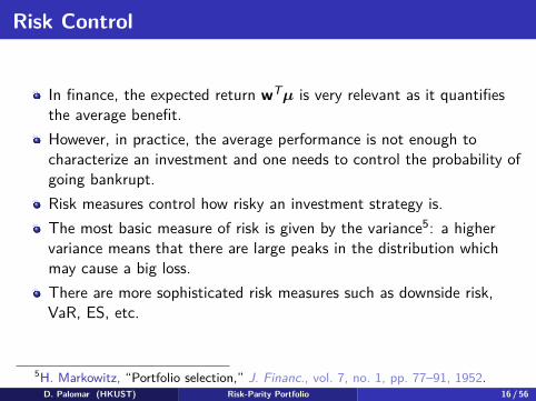
Risk Control

In finance, the expected return wTµ is very relevant as it quantifiesthe average benefit.However, in practice, the average performance is not enough tocharacterize an investment and one needs to control the probability ofgoing bankrupt.Risk measures control how risky an investment strategy is.The most basic measure of risk is given by the variance5: a highervariance means that there are large peaks in the distribution whichmay cause a big loss.There are more sophisticated risk measures such as downside risk,VaR, ES, etc.


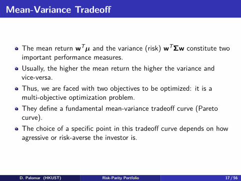
Mean-Variance Tradeoff

The mean return wTµ and the variance (risk) wTΣw constitute twoimportant performance measures.Usually, the higher the mean return the higher the variance andvice-versa.Thus, we are faced with two objectives to be optimized: it is amulti-objective optimization problem.They define a fundamental mean-variance tradeoff curve (Paretocurve).The choice of a specific point in this tradeoff curve depends on howagressive or risk-averse the investor is.


Markowitz mean-variance portfolio (1952)

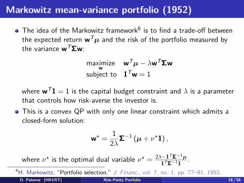
The idea of the Markowitz framework6 is to find a trade-off betweenthe expected return wTµ and the risk of the portfolio measured bythe variance wTΣw:

maximizew

wTµ− λwTΣwsubject to 1Tw = 1

where wT1 = 1 is the capital budget constraint and λ is a parameterthat controls how risk-averse the investor is.This is a convex QP with only one linear constraint which admits aclosed-form solution:

w⋆ = 12λ

Σ−1 (µ + ν⋆1) ,

where ν⋆ is the optimal dual variable ν⋆ = 2λ−1TΣ−1µ1TΣ−11 .


Global Minimum Variance Portfolio (GMVP)

The global minimum variance portfolio (GMVP) ignores the expectedreturn and focuses on the risk only:

minimizew

wTΣwsubject to 1Tw = 1.

It is a simple convex QP with solution

wGMVP = 11TΣ−11

Σ−11.

It is widely used in academic papers for simplicity of evaluation andcomparison of different estimators of the covariance matrix Σ (whileignoring the estimation of µ).


Outline

1 Introduction





4 Conclusions

Drawbacks of Markowitz’s formulation


1 variance is not a good measure of risk in practice since it penalizesboth the unwanted high losses and the desired low losses: the solutionis to use alternative measures for risk, e.g., VaR and CVaR,

2 it is highly sensitive to parameter estimation errors (i.e., to thecovariance matrix Σ and especially to the mean vector µ): solution isrobust optimization,

3 it only considers the risk of the portfolio as a whole and ignores the riskdiversification (i.e., concentrates risk too much in few assets, this wasobserved in the 2008 financial crisis): solution is the risk-parityportfolio.

We will here address the risk diversification among the as-sets by totally changing the portfolio formulation (and some-how address the sensitivity w.r.t. parameters).


Outline

1 Introduction





4 Conclusions

Motivation


it only considers the risk of the portfolio as a whole and ignores the riskdiversification (i.e., concentrates risk too much in few assets, this wasobserved in the 2008 financial crisis)it is highly sensitive to the estimation errors in the parameters (i.e.,small estimation errors in the parameters may change completely thedesigned portfolio)

Recently, the alternative risk parity portfolio design has beenreceiving significant attention from both the theoretical and practicalsides because

diversifies the risk, instead of the capital, among the assetsless sensitive to parameter estimation errors.


Outline

1 Introduction





4 Conclusions

Risk Contribution

Given a portfolio w ∈ RN and the return covariance matrix Σ, theportfolio volatility is:

σ (w) =√

wTΣw.

Following Euler’s theorem, the volatility can be decomposed asfollows:

σ (w) =N∑

i=1wi

∂σ

∂wi=

N∑i=1

wi (Σw)i√wTΣw

Risk contribution from asset i to the total risk σ (w):

wi∂σ

∂wi= wi (Σw)i√

wTΣw

Normalized risk contribution: wi (Σw)i /wTΣw

Other measures of risk f(w) like VAR and CVaR can also bedecomposed following Euler’s theorem.



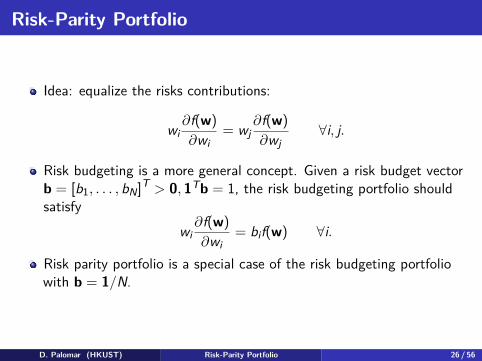
Idea: equalize the risks contributions:

wi∂f(w)∂wi

= wj∂f(w)∂wj

∀i, j.

Risk budgeting is a more general concept. Given a risk budget vectorb = [b1, . . . , bN]T > 0, 1Tb = 1, the risk budgeting portfolio shouldsatisfy

wi∂f(w)∂wi

= bif(w) ∀i.

Risk parity portfolio is a special case of the risk budgeting portfoliowith b = 1/N.



For the volatility we can writerisk parity: wi (Σw)i = wj (Σw)jrisk budgeting: wi (Σw)i = biwTΣw

Assuming that Σ is diagonal and with the constraints 1Tw = 1 andw ≥ 0, the risk budgeting portfolio is

wi =√

bi/√

Σii∑Nk=1√

bk/√

Σkk, i = 1, . . . , N.

However, for non-diagonal Σ or with other additional constraints, aclosed-form solution does not exist in general and some optimizationprocedures have to be constructed.The previous diagonal solution can always be used and is called naiverisk budgeting portfolio.



Consider the risk budgeting equations

wi (Σw)i = bi wTΣw, i = 1, . . . , N

with 1Tw = 1 and w ≥ 0.If we define x = w/

√wTΣw, then we can rewrite the risk budgeting

equations compactly asΣx = b/x

with x ≥ 0 and we can always recover the portfolio by normalizing:w = x/(1Tx).Spinu7 realized that precisely that equation corresponds to thegradient of the function f(x) = 1

2xTΣx− bT log(x) set to zero, whichis the optimality condition.Indeed, ∇f(x) = Σx− b/x.

7F. Spinu, “An algorithm for computing risk parity weights,” SSRN, 2013. [Online].Available: https://ssrn.com/abstract=2297383.


https://ssrn.com/abstract=2297383


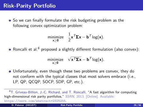
So we can finally formulate the risk budgeting problem as thefollowing convex optimization problem:

minimizex≥0

12xTΣx− bT log(x).

Roncalli et al.8 proposed a slightly different formulation (also convex):

minimizex≥0

√xTΣx− bT log(x).

Unfortunately, even though these two problems are convex, they donot conform with the typical classes that most solvers embrace (i.e.,LP, QP, QCQP, SOCP, SDP, GP, etc.).

8T. Griveau-Billion, J.-C. Richard, and T. Roncalli, “A fast algorithm for computinghigh-dimensional risk parity portfolios,” SSRN, 2013. [Online]. Available:https://ssrn.com/abstract=2325255.


https://ssrn.com/abstract=2325255


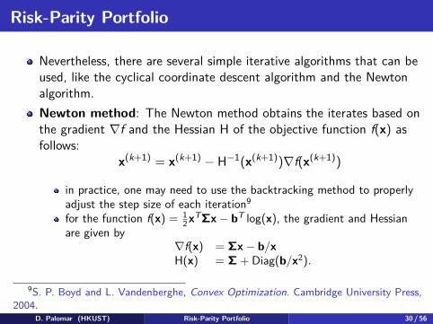
Nevertheless, there are several simple iterative algorithms that can beused, like the cyclical coordinate descent algorithm and the Newtonalgorithm.Newton method: The Newton method obtains the iterates based onthe gradient ∇f and the Hessian H of the objective function f(x) asfollows:

x(k+1) = x(k+1) − H−1(x(k+1))∇f(x(k+1))

in practice, one may need to use the backtracking method to properlyadjust the step size of each iteration9

for the function f(x) = 12 xTΣx− bT log(x), the gradient and Hessian

are given by∇f(x) = Σx− b/xH(x) = Σ + Diag(b/x2).

9S. P. Boyd and L. Vandenberghe, Convex Optimization. Cambridge University Press,2004.



Cyclical coordinate descent algorithm: This method simplyminimizes in a cyclical manner with respect to each element of thevariable x.

the minimization w.r.t. xi is

minimizexi≥0

12x2

i σ2i + xi(xT

−iΣ:,i)− bi log xi

with gradient∇if = xiσ

2i + (xT

−iΣ:,i)− bi/xi

setting the gradient to zero gives us the second order equation

x2i σ2

i + xi(xT−iΣ:,i)− bi = 0

with positive solution given by

x⋆i =−(xT

−iΣ:,i) +√

(xT−iΣ:,i)2 + 4σ2

i bi

2σ2i

.



These methods are very nice and they will converge to the optimalrisk budgeting solution (because the problem formulated was convex).However, they can only be employed for the simplest risk budgetingformulation with a simplex constraint set (i.e., 1Tw = 1 and w ≥ 0).They cannot be used if

we have other constraints like allowing shortselling or box constraints:li ≤ wi ≤ ion top of the risk budgeting constraints wi (Σw)i = bi wTΣw we haveother objectives like maximizing the expected return wTµ orminimizing the overall variance wTΣw.

In those more general cases, we need more sophisticated formulations,which unfortunately will not be convex.In the R programming language there is a package calledriskParityPortfolio that can solve very efficiently all the formulations.


https://github.com/dppalomar/riskParityPortfolio

Risk-Parity Formulation

Maillard et al.10 aimed at solving:

minimizew

∑Ni,j=1

(wi (Σw)i − wj (Σw)j

)2

subject to 1Tw = 1.

The idea is to try to achieve equal risk contributions wi(Σw)i√wTΣw

bypenalizing the differences between the terms wi (Σw)i.This is a simplified formulation:

minimizew,θ

∑Ni=1 (wi (Σw)i − θ)2

subject to 1Tw = 1.

10S. Maillard, T. Roncalli, and J. Teïletche, “The properties of equally weighted riskcontribution portfolios,” Journal of Portfolio Management, vol. 36, no. 4, pp. 60–70,2010.


More Risk-Parity Formulations

Bruder and Roncalli11 proposed to solve:

minimizew

∑Ni=1

(wi(Σw)iwTΣw − bi

)2

subject to wT1 = 1,

where bi = 1N .

More generally, one can equalize the risk contribution by settingarbitrary proportions (as opposed to equal contributions):

b = [b1, . . . , bN]T > 0, 1Tb = 1.

One more formulation:minimize

w∑N

i,j=1

(wi(Σw)i

bi− wj(Σw)j

bj

)2

subject to 1Tw = 1.

11B. Bruder and T. Roncalli, “Managing risk exposures using the risk budgetingapproach,” University Library of Munich, Germany, Tech. Rep., 2012.


And Yet More Risk-Parity Formulations

One more formulation:

minimizew

∑Ni=1

(wi (Σw)i − biwTΣw

)2

subject to 1Tw = 1.

And one more:

minimizew

∑Ni=1

( wi(Σw)i√wTΣw

− bi√

wTΣw)2

subject to 1Tw = 1.


Yet Even More Risk-Parity Formulations

What about this one:

minimizew,θ

∑Ni=1

(wi(Σw)ibi− θ

)2

subject to 1Tw = 1.

More formulations can be found in the book:T. Roncalli, Introduction to Risk Parity and Budgeting. CRC Press,2013.


General Problem Formulation

A more general risk parity formulation is12:

minimizew

U (w) ≜ ∑Ni=1 (gi (w))2 + λF (w)

subject to 1Tw = 1, w ∈ W

where∑Ni=1 (gi (w))2: risk concentration measurement, e.g.,

gi (w) ≜ wi (Σw)iwTΣw − 1

N ,

F (w): preference, e.g., 0, −µTw, −µTw + νwTΣw,λ ≥ 0: trade-off parameter,1Tw = 1, w ∈ W: capital budget & other convex constraints.

Challenge: the problem is highly nonconvex due to ∑Ni=1 (gi (w))2.

12Y. Feng and D. P. Palomar, “SCRIP: Successive convex optimization methods forrisk parity portfolios design,” IEEE Trans. Signal Process., vol. 63, no. 19,pp. 5285–5300, 2015.


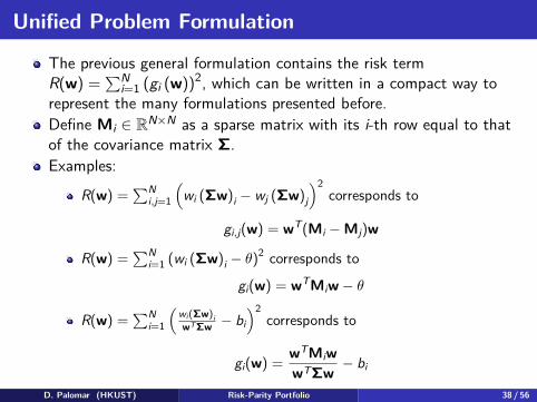
Unified Problem Formulation

The previous general formulation contains the risk termR(w) =

∑Ni=1 (gi (w))2, which can be written in a compact way to

represent the many formulations presented before.Define Mi ∈ RN×N as a sparse matrix with its i-th row equal to thatof the covariance matrix Σ.Examples:

R(w) =∑N

i,j=1

(wi (Σw)i − wj (Σw)j

)2corresponds to

gi,j(w) = wT(Mi −Mj)w

R(w) =∑N

i=1 (wi (Σw)i − θ)2 corresponds to

gi(w) = wTMiw− θ

R(w) =∑N

i=1

(wi(Σw)iwTΣw − bi

)2corresponds to

gi(w) = wTMiwwTΣw − bi


Unified Problem Formulation

More examples:

R(w) =∑N

i,j=1

(wi(Σw)i

bi− wj(Σw)j

bj

)2corresponds to

gi,j(w) = wT(Mi/bi −Mj/bj)w

R(w) =∑N

i=1(wi (Σw)i − biwTΣw

)2 corresponds to

gi(w) = wT(Mi − biΣ)w

R(w) =∑N

i=1

(wi(Σw)i√

wTΣw− bi√

wTΣw)2

corresponds to

gi(w) = wTMiw√wTΣw

− bi√

wTΣw

R(w) =∑N

i=1

(wi(Σw)i

bi− θ

)2corresponds to

gi(w) = wTMiw/bi − θ


Outline

1 Introduction





4 Conclusions

Numerical Solving Approach

Some off-the-shelf nonlinear numerical optimization methods13 aretypically used, e.g.,

Sequential Quadratic Programming (SQP)Interior Point Methods (IPM).

For such risk-parity portfolio problems, theymay be very slow, andget stuck at some unsatisfactory points.

Because the structure of the objective is not explored.

13J. Nocedal and S. J. Wright., Numerical Optimization, Second. Springer Verlag,2006.


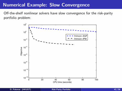
Numerical Example: Slow ConvergenceOff-the-shelf nonlinear solvers have slow convergence for the risk-parityportfolio problem:

0 20 40 60 80 10010

−12

10−10

10−8

10−6

10−4

10−2

100

102

CPU time (seconds)

Obje

ctive

fmincon−SQP

fmincon−IPM


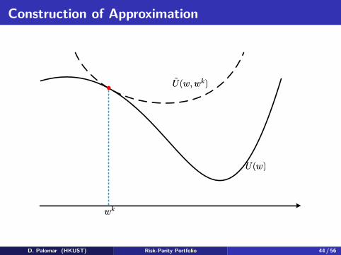
Successive Convex Approximation (SCA)

Basic idea: solving a difficult problem via solving a sequence ofsimpler problems.Minimize U (w) over w ∈ W via SCA method14:

Construction of Approximation: finding U(w; wk)

that approximatesthe function U (w) at the point wk and

U(w; wk): uniformly strongly convex & cont. differentiable

∇U(w; wk): Lipschitz continuous on W

∇U(w; wk) |w=wk = ∇U (w) |w=wk

Minimization: minimizing U(w; wk)

to get the update

wk+1 ≜ arg minw∈W

U(w; wk)

.

14G. Scutari, F. Facchinei, P. Song, D. P. Palomar, and J.-S. Pang, “Decompositionby partial linearization: Parallel optimization of multi-agent systems,” IEEE Trans.Signal Process., vol. 62, no. 3, pp. 641–656, 2014.


Construction of Approximation


Minimization


One More Iteration


Classical Methods as SCA

(Unconstrained) gradient descent: Set

U(w; wk

)= U

(wk

)+∇U

(wk

)T (w−wk

)+ 1

2αk

∥∥∥w−wk∥∥∥2

2.

Setting the derivative w.r.t. w to zero yields:

wk+1 = wk − αk∇U(wk

).

(Unconstrained) Newton’s method: Set

U(w; wk

)= U

(wk

)+∇U

(wk

)T (w−wk

)+ 1

2αk

(w−wk

)T∇2U

(wk

) (w−wk

).

Setting the derivative w.r.t. w to zero yields:

wk+1 = wk − αk(∇2U

(wk

))−1∇U

(wk

).


SCA for Risk Parity Portfolio Design

Recall the objective

U (w) =N∑

i=1(gi (w))2 + λF (w) .

At the k-th iteration wk, set τ > 0 and construct

U(w, wk

)=

P(w;wk)≜︷︸︸︷N∑

i=1

(gi

(wk

)+

(∇gi

(wk

))T (w−wk

))2

+τ

2∥∥∥w−wk

∥∥∥2

2+ λF (w)

IDEA: linearizing nonconvex functions gi (w) inside the least square=⇒ quadratic convex P

(w; wk

)approximates

R(w) =∑N

i=1 (gi (w))2, with ∇P(w, wk

)|w=wk = ∇R (w) |w=wk .


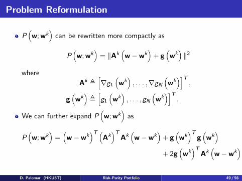
Problem Reformulation

P(w; wk

)can be rewritten more compactly as

P(w; wk

)= ∥Ak

(w−wk

)+ g

(wk

)∥2

whereAk ≜

[∇g1

(wk

), . . . ,∇gN

(wk

)]T,

g(wk

)≜

[g1

(wk

), . . . , gN

(wk

)]T.

We can further expand P(w; wk

)as

P(w; wk

)=

(w−wk

)T (Ak

)TAk

(w−wk

)+ g

(wk

)Tg

(wk

)+ 2g

(wk

)TAk

(w−wk

)D. Palomar (HKUST) Risk-Parity Portfolio 49 / 56

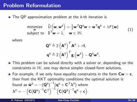
Problem Reformulation

The QP approximation problem at the k-th iteration is

minimizew

U(w, wk

)= 1

2wTQkw + wTqk + λF (w)subject to 1Tw = 1, w ∈ W.

(1)

whereQk ≜ 2

(Ak

)TAk + τ I,

qk ≜ 2(Ak

)Tg

(wk

)−Qkwk,

This problem can be solved direclty with a solver or, depending on theconstraints in W, one may derive simpler closed-form solutions.For example, if we only have equality constraints in the form Cw = c,then from the KKT optimality conditions the optimal solution isfound as wk = −(Qk)−1(qk + CTλk) whereλk = −

(C(Qk)−1CT

)−1 (C(Qk)−1qk + c

).


Sequential Numerical AlgorithmAlgorithm 1: Successive Convex optimization for RIsk Parityportfolio (SCRIP).Set k = 0, w0 ∈ W, τ > 0, {γk} ∈ (0, 1]repeat

Solve QP problem (1) to get the optimal solution wk (globalminimum)wk+1 = wk + γk

(wk −wk

)k← k + 1

until convergencereturn wk

More advanced algorithms can be found inY. Feng and D. P. Palomar, “SCRIP: Successive convex optimizationmethods for risk parity portfolios design,” IEEE Trans. SignalProcess., vol. 63, no. 19, pp. 5285–5300, 2015.


Convergence Analysis

Proposition 1Under some technical conditions, suppose τ > 0, γk ∈ (0, 1], γk → 0,∑

k γk = +∞ and ∑k

(γk

)2< +∞, and let

{wk

}be the sequence

generated by Algorithm 1. Then, either Algorithm 1 converges in a finitenumber of iterations to a stationary point or every limit of

{wk

}(at least

one such point exists) is a stationary point.


Numerical exampleFast algorithms based on successive convex approximation (SCA):

0 20 40 60 80 10010

−12

10−10

10−8

10−6

10−4

10−2

100

102

CPU time (seconds)

Obje

ctive

fmincon−SQP

fmincon−IPM

SCRIP

0 0.2 0.4 0.6 0.8

10−10

10−5

100


Outline

1 Introduction





4 Conclusions

Conclusions

We have reviewed the Markowitz portfolio formulation andunderstood that it has many practical flaws that make it impractical.Indeed, it is not used by practitioners.

We have learned about the risk-parity portfolio formulation.

We have explored the numerical resolution of such problems viasuccessive convex approximation (SCA) methods.

The performance of risk-parity portfolio versus Markowitz portfolio ismuch improved.

Side result: we have learned how to develop efficient numericalalgorithms based on SCA.


Thanks

For more information visit:

https://www.danielppalomar.com

risk-parity portfolio 10/slides_risk... · the expected return wtµ and the risk of the portfolio...

Documents