r/maanova: an extensive r environment for the analysis of...
TRANSCRIPT

R/MAANOVA: An extensive R environment for theAnalysis of Microarray Experiments
Hao Wu, Gary A. Churchill
April 17, 2007
Contents
1 Introduction 2
2 Installation 32.1 System requirements . . . . . . . . . . . . . . . . . . . . . . . . . . . . . 32.2 Obtaining R . . . . . . . . . . . . . . . . . . . . . . . . . . . . . . . . . . 32.3 Installation - Windows(9x/NT/2000) . . . . . . . . . . . . . . . . . . . . 32.4 Installation - Linux/Unix . . . . . . . . . . . . . . . . . . . . . . . . . . . 3
3 Data and function list 5
4 Preparing the input files 74.1 Preparing the data file . . . . . . . . . . . . . . . . . . . . . . . . . . . . 74.2 Preparing the design file . . . . . . . . . . . . . . . . . . . . . . . . . . . 8
5 A quick tour of the functions 95.1 CAMDA kidney experiment . . . . . . . . . . . . . . . . . . . . . . . . . 95.2 Paigen’s 300-gene experiment . . . . . . . . . . . . . . . . . . . . . . . . 205.3 An affymetric experiment . . . . . . . . . . . . . . . . . . . . . . . . . . 22
A Running R/maanova on computer cluster 25A.1 System requirements . . . . . . . . . . . . . . . . . . . . . . . . . . . . . 25A.2 System setup . . . . . . . . . . . . . . . . . . . . . . . . . . . . . . . . . 25A.3 Install and test clusters in R . . . . . . . . . . . . . . . . . . . . . . . . . 26
B Basic Algorithms 27B.1 ANOVA model for microarray experiment . . . . . . . . . . . . . . . . . 27
B.1.1 Model . . . . . . . . . . . . . . . . . . . . . . . . . . . . . . . . . 27B.1.2 Fixed model versus Mixed model . . . . . . . . . . . . . . . . . . 27
1

B.2 Hypothesis tests . . . . . . . . . . . . . . . . . . . . . . . . . . . . . . . . 28B.2.1 F test in matrix notation . . . . . . . . . . . . . . . . . . . . . . . 28B.2.2 Building L matrix . . . . . . . . . . . . . . . . . . . . . . . . . . . 29B.2.3 Four flavors of F-tests . . . . . . . . . . . . . . . . . . . . . . . . 29
B.3 Data shuffling in permutation test . . . . . . . . . . . . . . . . . . . . . . 30
C Frequently Asked Questions 31
1 Introduction
R/maanova is an extensible, interactive environment for the analysis of microarray ex-periments. It is implemented as an add-on package for the freely available statisticallanguage R (www.r-project.org). The engine functions were written in C for betterperformance.
MAANOVA stands for MicroArray ANalysis Of VAriance. It provides a completework flow for microarray data analysis including:
• Data quality checks and visualization
• Data transformation
• ANOVA model fitting for both fixed and mixed effects models
• Statistical tests including permutation
• Cluster analysis with bootstrapping
R/maanova can be applied to any microarray data but it is specially tailored formultiple factor experimental designs. Mixed effects models are implemented to estimatevariance components and perform F and T tests for differential expressions.
2

2 Installation
2.1 System requirements
This package was developed under R 1.8.0 in the Linux Redhat 8.0 operating system.The programs have been observed to work under Windows NT/98/2000. The memoryrequirement depends on the size of the input data but a minimum of 256Mb memory isrecommended.
2.2 Obtaining R
R is available in the Comprehensive R Archive Network (CRAN). Visithttp://cran.r-project.org or a local mirror site. Source code is available for UNIX/LINUX,and binaries are available for Windows, MacOS, and many versions of Linux.
2.3 Installation - Windows(9x/NT/2000)
• Install R/maanova from Rgui
1. Start Rgui
2. Select Menu Packages, click Install package from local zip file. Choosethe filemaanova_*.tar.gz and click ’OK’.
• Install R/maanova outside Rgui
1. Unzip the maanova_*.tar.gz file into the directory $RHOME/library ($RHOMEis something like c:/Program Files/R/rw1081). Note that this should createa directory$RHOME/library/maanova containing the R source code and the compileddlls.
2. Start Rgui.
3. Type link.html.help() to get the help files for the maanova package addedto the help indices.
2.4 Installation - Linux/Unix
1. Go into the directory containing maanova_*.tar.gz.
2. Type R CMD INSTALL maanova to have the package installed in the standard lo-cation such like /usr/lib/R/library. You will have to be the superuser to dothis. As a normal user, you can install the package in your own local directory. Todo this, type R CMD INSTALL -library=$LOCALRLIB maanova_*.tar.gz, where
3

$LOCALRLIB is something like /home/user/Rlib/. Then you will need to create afile .Renviron in your home directory to contain the line R_LIBS=/home/user/Rlibso that R will know to search for packages in that directory.
4

3 Data and function list
The following is a list of the available functions. For more information about the func-tion usage use the online help by typing “?functionname” in R environment or typinghelp.start() to get the html help in a web browser.
1. Sample data available with the package
abf1 A 18-array affymetric experiment. 500 hand picked genes are included in thedata set
kidney A 6-array kidney data set from CAMDA (Critical Assessment of Microar-ray Data Analysis).
paigen A multiple factor 28-array experiment from Bev Paigen’s lab in The Jack-son Lab. Only 300 hand picked genes are included in this data set
2. File I/O
read.madata Read microarray data from TAB delimited simplex text file.
write.madata Write microarray data to a TAB delimited simple text file.
3. Data quality check
arrayview View the layout of the arrays
riplot Ratio intensity plot for arrays
gridcheck Plot grid-by-grid data comparison for arrays
dyeswapfilter Flag the bad spots in dye swap experiment Note that these dataquality check functions only work for 2-dye arrays at this time.
4. Data transformation
createData Create a data object with options to collapse the replicated spots anddo log2 transformation
transform.madata Data transformation with options to use any of several meth-ods
5. ANOVA model fitting
makeModel Make model object to represent the experimental design
fitmaanova Fit ANOVA model
resiplot Residual plot on a given ANOVA model
6. Hypothesis testing
5

matest F-test or T-test with permutation
adjPval Calculate FDR adjusted P values given the result of [matest]
volcano Volcano plot for summarizing F or T test results
7. Clustering
macluster Bootstrap clustering.
consensus Build consensus tree out of bootstrap cluster result
fom Use figure of merit to determine the number of groups in K-means cluster
geneprofile Plot the estimated relative expression for a given list of genes
8. Utility functions
fill.missing Fill in missing data.
summary.madata Summarize the data object.
summary.mamodel Summarize the model object.
subset.madata Subsetting the data objects.
exprSet2Rawdata Convert an object of exprSet to an object of Rawdata.
6

4 Preparing the input files
Before using the package, the user must manually prepare a data file and a design file.
4.1 Preparing the data file
There is only ONE data file for all of the slides in an experiment. Most gridding soft-ware produces one file for each slide. Thus you will have multiple files for a multiplearray experiment and you have to combine these files to one data file as the input forR/maanova.
The data file is a TAB delimited text file. Each rows corresponds to the data for agene. In the first a few columns, you can put some gene information, e.g., the Clone ID,Gene Bank ID, etc. and the grid location of the spot. Note that some gridding soft-wares return Block numbers instead of metarow and metacol. Then you must manuallycompute metarow and metacol from block and put them in the file. After that you needto put the scanned data for all arrays in the rest of the columns. (You need to make thedecision what data you want to use in analysis, e.g., mean versus median, backgroundsubtracted or not, etc.) For N-dye arrays, the N channel intensity data for one arrayneed to be adjacent to each other (in consecutive columns). The order (dye1, dye2, ...)must be consistent across all of the slides. You can put the spot flag as a column afterintensity data for each array. (Note that if you have flag, you will have N+1 columns ofdata for each array. Again, this must be consistent for all arrays in the data set.) If youhave duplicated spots within one array, replicated measurements of the same clone onthe same array should appear in adjacent rows. This can be easily done by sorting oncloneid. The number of replicates must be constant for all genes.
As an example, you have four slides for a 2-dye array experiment scanned by GenePix.Then you will have four output files. Following the steps to create your data file:
1. Open your favorite spread sheet editor, e.g., MS Excel and create a new file;
2. Paste your clone ID, Gene names, Cluster ID and whatever information you wantto keep into the first several columns;
3. Open your first GenePix file in another window, copy the grid location into next4 columns (you only need to do this once because they are all the same for fourslides);
4. Copy the two columns of foreground mean value (if you want to use it) and onecolumn of flag to the file in the order of Cy5, Cy3, flag;
5. Open your other 3 files and repeat step 4;
6. Select the whole file and row sort it according to Clone ID;
7. Save the file as tab delimited text file and you are done.
7

The data file must be “full”, that is, all rows have to have same number of columns.Sometimes leading and trailing TAB in the text file can cause problems, depending onthe operating system. So the user should be careful about that. Sometimes the specialcharacters in gene description can cause reading problem. I don’t encourage you toput the gene description in the data file. If you have to do that, you must be careful(sometimes you need to remove the special characters manually).
4.2 Preparing the design file
The design file is another TAB delimited text file. The number of rows in this file equalsthe number of arrays times N(the number of dyes) plus one (for the column headers).The number of columns in this file depends on the experimental design. For example,you can have“Strain”, “Diet”, “Sex”, etc. in your design file. You must have the followingcolumns in the design file (column headers are case sensitive):
• Array: for array name
• Dye: for dye name
• Sample: Sample ID number
Array and Dye columns are easy to understand. Sample column contains integers usedto identify biological replicates and reference samples. Usually you should assign eachbiological individual a unique Sample number. Reference samples are represented byzero(0). Reference sample are treated differently. They will always be treated as fixedfactor in the model and not involved in statistical tests.
You must not have the following columns in the design file:
• Spot: reserved for spot effect
• Label: reserved for labelling effect
Sample column in design file need to be continuous integer. All other columns canbe either integers or characters.
You don’t have to USE all factors in design file. When making the model object inmakeModel, the experimental design will be determined by the design and a formula.You can put all factors in design file but turn them on/off in formula.
8

5 A quick tour of the functions
This section will go through a few demo scripts distributed with the package to help theusers understand the function syntax and capabilities. The binary data are distributedwith the software. The original data file can be downloaded from:http://www.jax.org/staff/churchill/labsite/software/
5.1 CAMDA kidney experiment
This is the kidney data from CAMDA (Critical Assessment of Microarray Data Analysis)originally described by Pritchard et al.
The website for CAMDA is http://www.camda.duke.edu. It is a 24-array doublereference design. Six samples are compared to a reference with dye swapped and allarrays are duplicated. Flag for bad spots is included in the data.
Note that because BioConductor requires all contributed packages to be less than1Mb in size, the binary data distributed with the package is only a small part of the realdata set (first 300 genes). So you cannot reproduce the figures presented in followingsections. The package with full data set, can be download from Gary Churchill’s websiteat http://www.jax.org/staff/churchill/labsite/software/. You can also find theoriginal data file (in text format) there.
1. First load data into the workspace
R> data(kidney)
2. Then we do some data quality check
R> gridcheck(kidney.raw)
gridcheck is used to check the hybridization and gridding quality within and crossarrays. You should see near linear scatter plots in all grid for all arrays. This oneis not great but acceptable. The grid check plot for the first array is shown infigure 1. The red dots are for the spots with flags.
R> riplot(kidney.raw)
riplot stands for ratio-intensity plot. It is also called MA plot. The riplot for thefirst array is shown in figure 2.
R> arrayview(kidney.raw)
arrayview is used to view the spatial pattern of the arrays. The standardized logratios for all spots are shown in different colors. The arrayview for the first arrayis shown in figure 3.
You will generate a lot of figures by doing gridcheck, riplot and arrayview. Usegraphics.off to close all figures.
9

Figure 1: Grid check plot for the first array in kidney data
10
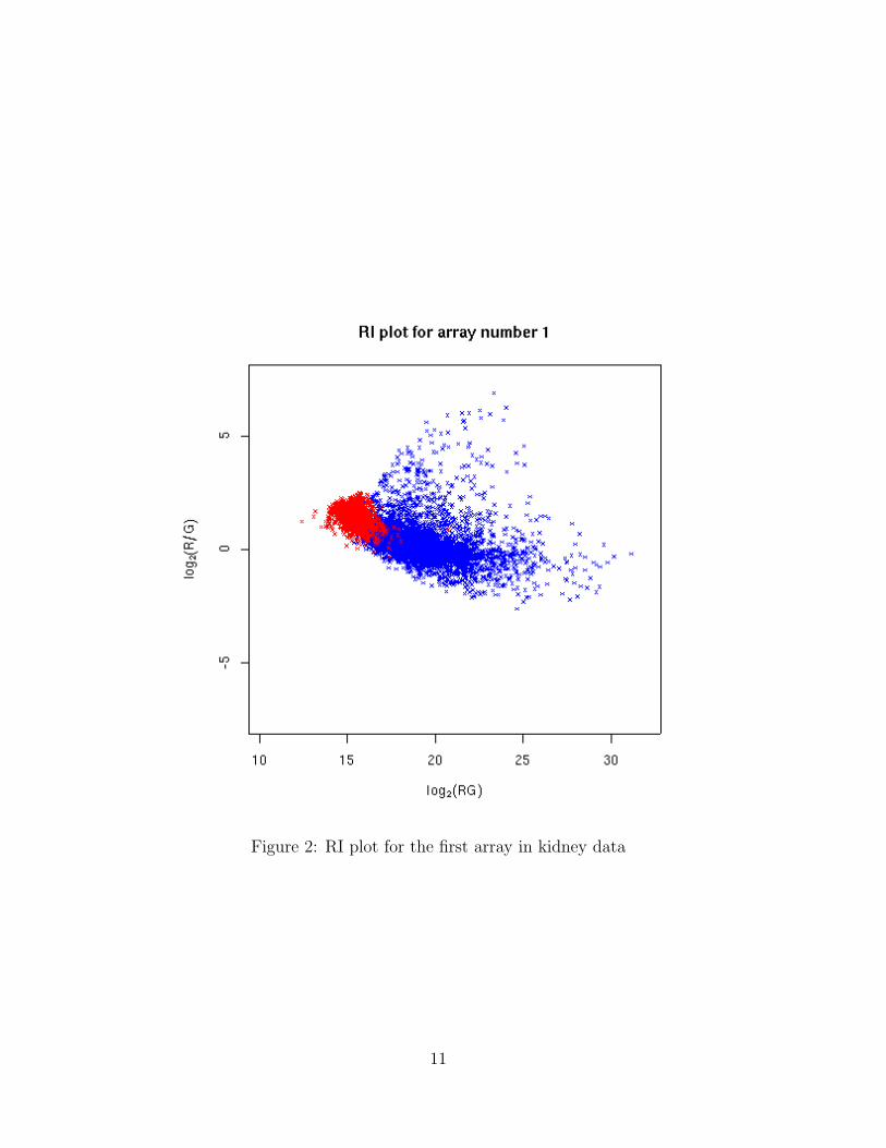
Figure 2: RI plot for the first array in kidney data
11
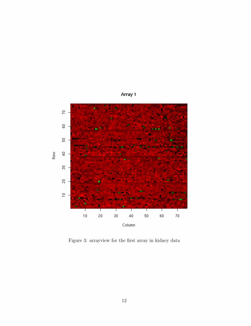
Figure 3: arrayview for the first array in kidney data
12

3. Now make an object of class madata. madata and mamodel are the key objectsin R/maanova. Most of the functions work on them. A madata object stores theexperimental data. It derived from the raw data. The mamodel object stores theexperimental design information. We will discuss it a little later.
R> kidney <- createData(kidney.raw)
R> summary(kidney)
4. Transform the data using spatial-intensity joint loess.
R> kidney <- transform.madata(kidney, method="rlowess")
There are several data transformation method. Which method to use depends onthe data. Read Cui et al.(2002) for detail. The transformation plot for the firstarray is shown in figure 4.
Figure 4: Joint lowess transformation on the first array for the kidney data
13

5. Make model object for fixed model
R> model.fix <- makeModel(data=kidney, formula=~Dye+Array+Sample)
R> summary(model.fix)
A mamodel object store the experimental design information. makeModel functiontakes a data object and a R formula as the ANOVA model and make the designmatrices. The input formula is an object of formula. It represents the ANOVAmodel. In the formula, you can put any combination of the factors in your design.Interaction between any two terms are allowed. At this point, 3 or higher wayinteractions are not taken by the program. makeModel takes another argumentrandom for the random terms. random must be another formula. All terms inrandom must be included in formula as well.
6. Fit ANOVA model and do residual plot
R> anova.fix <- fitmaanova(kidney, model.fix)
R> resiplot(kidney, anova.fix)
7. Permutation F test. F-test function can test one or multiple terms in a given modelobject. User can do residual shuffling or sample shuffling for fixed effect models.For mixed effects models, only sample shuffling is available. Permutation test couldbe very time consuming, especially for mixed effects models. The permutationtest function can run on linux clusters through message passing interface (MPI).For detailed information about F test and using computer cluster, please readappendix.
Here we want to test Sample effect in the model:
R> test.fix <- matest(kidney, model=model.fix, term="Sample",
n.perm=500)
Now test.fix contains the tabulated P values and permutaion P values. Some-times we want to calculate FDR adjusted P values for the test result.
R> test.fix <- adjPval(test.fix)
After getting the F-test result, We can do volcano plot to visualize it. volcano
function has options to choose the P-values to use and set up thresholds. We willuse tabulated P values for F1 and FDR adjusted permutation P values for othertests here. In the plot, the orange dots above the horizontal line represent thesignificant genes. Note that the the flagged spot can be highlighted in the plot.You can turn if on by providing highlight.flag=TRUE.
R> idx.fix <- volcano(test.fix,method=c("unadj", rep("fdrperm",3)),
highlight.flag=FALSE)
14

Figure 5: Volcano plot for kidney data - fixed effect model
15

The volcano plot is shown in figure 5. Note that the return variable of volcanocontains the indices for significant genes.
8. Now we can do cluster bootstrapping and build consensus trees. Currently twocluster methods are implemented, hierarchical clustering and K-means. Hierar-chical cluster could be very sensitive to bootstrap if you have too many leaveson the cluster. Some small disturbance on the data could change the whole treestructure. So if you have many genes, say, more than 50, and you want to build aconsensus tree from 100 bootstrapped hierarchical trees. It is very likely that youget a comb, that is, all leaves are directly under root. But if you only have a fewgenes to cluster, it is working fine. So I suggest user use K-means to cluster thegenes and use hierarchical to cluster the samples.
macluster is the function to do cluster bootstrapping and consensus is used tobuild consensus trees (groups for K-means) from the bootstrap results.
R> cluster.kmean <- macluster(anova.fix, ,term="Sample",
idx.gene=idx.fix$idx.all,what="gene", method="kmean"
kmean.ngroups=5, n.perm=100)
R> con.kmean <- consensus(cluster.kmean, 0.7)
An expression profile plot will be generated for the consensus K-means result. Theplot is shown in figure 6.
Now we can do hierarchical cluster on the samples. The consensus tree is shownin figure 7.
R> cluster.hc <- macluster(anova.fix, term="Sample",
idx.gene=idx.fix$idx.all,what="sample", method="hc", n.perm=100)
R> con.hc <- consensus(cluster.hc)
9. Now we are going to analyze the data using mixed effect model. First we make amodel object with Array effect as random factor. Note that normally Array effect,Spot effect and Labeling effect should be treated as random. Since we don’t havetechnical replicate here, Spot and Label cannot be fitted.
R> model.mix <- makeModel(data=kidney, formula=~Dye+Array+Sample,
random=~Array)
R> summary(model.mix)
10. Then we can fit the ANOVA model. This will take quite a while to finish. EMalgorithm is implemented in the engine function for solving MME. For detailsabout MME and the EM algorithms, read Searle et al..
R> anova.mix <- fitmaanova(kidney, model.mix)
16

1 2 3 4 5 6
−0.5
0.5
1.5
Expression profile for group 1 (9 genes)
Sample index
Exp
ress
ion
leve
l
1 2 3 4 5 6
−1.0
0.0
1.0
Expression profile for group 2 (10 genes)
Sample indexE
xpre
ssio
n le
vel
1 2 3 4 5 6
−0.5
0.5
Expression profile for group 3 (19 genes)
Sample index
Exp
ress
ion
leve
l
1 2 3 4 5 6
−1.0
0.0
1.0
Expression profile for group 4 (19 genes)
Sample index
Exp
ress
ion
leve
l
1 2 3 4 5 6
−0.5
0.5
Expression profile for group 5 (41 genes)
Sample index
Exp
ress
ion
leve
l
1 2 3 4 5 6
−1.0
0.0
1.0
Not in any group (32 genes)
Sample index
Exp
ress
ion
leve
l
Figure 6: Expression profile plot for bootstrap K-means result, kidney data
17

0.0 0.5 1.0 1.5 2.0 2.5 3.0
HC
samples (kidney data) − 80%
Consensus tree
depth
sample1
sample2
sample3
sample4
sample5
sample6
1.000.84
0.890.84
Figure 7: 80% Consensus tree for bootstrapping hierarchical cluster on the samples,kidney data
18

11. Now we test the sample effect. Again, permutation test for mixed effects model isvery slow. You have better run it on computer clusters if possible.
R> ftest.mix <- matest(data=kidney, model=model.mix, term="Sample",
n.perm=100)
We can do volcano plot for the mixed model result.
R> idx.mix <- volcano(anova.mix, ftest.mix)
The rest of the analysis (clustering and consensus trees) are skipped here.
19

5.2 Paigen’s 300-gene experiment
This is a multiple factor 28-array experiment. The experiment is done in Beverly Paigen’sLab in The Jackson Lab. They took three strains of mice and feed them with two kindof diets. In that way you get six kind of mice. They picked two individuals in eachgroup then you have totally 12 distinct mice. So in this experiment, you have strain,diet and biological replicates as the factors. You can test the effects from any factor orany combination of them. The experimental deign in shown in table 1 and figure 8.
Hi fat diet Low fat dietStrain:Pera A1, A2 E1, E2Strain:I B1, B2 F1, F2Strain:DBA C1, C2 D1, D2
Table 1: Mice used in Paigen’s 28-array experiment
F1
C1
D1
A1
B1
E1
F2
C2
D2
A2
B2
E2
Figure 8: Array assignment in Paigen’s 28-array experiment
We will skip the data quality check and transformation steps in this example. Wewill show you how to test different terms in the model in a multiple factor design. In thisdesign, there are strain effect, diet effect, strain by diet interaction effect and biologicalreplicate effect. The interaction effect is nested within the biological replicate effect.
1. Load in data
R> data(paigen)
2. Make data object with replicates collapsed. Note that if we donot collapse repli-cates, we need to put Spot in the model as a random terms. That will make thecalculation even slower. Based on our experience, collapsing replicates gives similarresults as not collapsing and fit Spot effect as random.
R> paigen <- createData(rawdata, 2, 1)
20

3. Make several model object and fit ANOVA. First make full model object withStrain, Diet, interaction and biological replicate effects.
R> model.full.mix <- makeModel(data=paigen,
formula=~Dye+Array+Strain+Diet+Strain:Diet,
random=~Array+Sample)
R> anova.full.mix <- fitmaanova(paigen, model.full.mix)
We can do a variance component plot on ANOVA result.
R> varplot(anova.full.mix)
Then make a model object without interaction effect and fit ANOVA model
R> model.noint.mix <- makeModel(data=paigen,
formula=~Dye+Array+Strain+Diet+Sample, random=~Array+Sample)
R> anova.noint.mix <- fitmaanova(paigen, model.noint.mix)
4. F test on different effects. First we want to test the interaction effect. The interac-tion effect must be tested in the full model. Note that because the interaction effectis nested within biological replicates, we have to use biorep to test the interaction.
R> ftest.int.mix <- matest(data=paigen, model=model.full.mix,
term="Strain:Diet")
R> idx.int.mix <- volcano(anova.full.mix, ftest.int.mix)
Then we want to test the Strain and Diet effect. We use the model withoutinteraction to test the main effect.
R> ftest.strain.mix <- matest(data=paigen, model=model.noint.mix,
term="Strain")
R> ftest.diet.mix <- matest(data=paigen, model=model.noint.mix,
term="Diet")
We can do volcano plot to visualize the F-test results and pick significant genes.That step is skipped here.
5. Now we can do T-test on any comparison on a given term. The result still containsthe F values (with numerator’s degree of freedom equals 1). To to do all pairwisecomparison on Strain, first make a comparison matrix:
R> C <- matrix(c(1,-1,0,1,0,-1, 0,1,-1), nrow=3, byrow=T)
Users need to be careful about specifing comparsion matrix. The comparison needto be the linear combination of the rows of the design matrix for fixed terms.Otherwise the comparision will be non-estimable.
To do the test:
21
R> ttest.strain <- matest(paigen, model.noint.mix, term="Strain",
Contrast=C, n.perm=500)
Because we have three comparisons here, doing volcano will generate three plots.
R> volcano(ttest.strain)
Again, the clustering analysis is skipped here.
5.3 An affymetric experiment
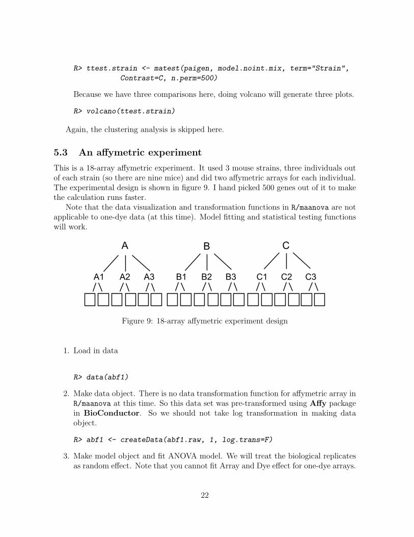
This is a 18-array affymetric experiment. It used 3 mouse strains, three individuals outof each strain (so there are nine mice) and did two affymetric arrays for each individual.The experimental design is shown in figure 9. I hand picked 500 genes out of it to makethe calculation runs faster.
Note that the data visualization and transformation functions in R/maanova are notapplicable to one-dye data (at this time). Model fitting and statistical testing functionswill work.
A B C
A1 A2 A3 B1 B2 B3 C1 C2 C3
Figure 9: 18-array affymetric experiment design
1. Load in data
R> data(abf1)
2. Make data object. There is no data transformation function for affymetric array inR/maanova at this time. So this data set was pre-transformed using Affy packagein BioConductor. So we should not take log transformation in making dataobject.
R> abf1 <- createData(abf1.raw, 1, log.trans=F)
3. Make model object and fit ANOVA model. We will treat the biological replicatesas random effect. Note that you cannot fit Array and Dye effect for one-dye arrays.
22

R> model.full.mix <- makeModel(data=abf1, formula=~Strain+Sample,
random=~Sample)
R> anova.full.mix <- fitmaanova(abf1, model.full.mix)
4. Do F-test on strain and generate volcano plot
R> test.Strain.mix <- matest(abf1, model.full.mix, term="Strain",
n.perm=100)
R> idx.mix <- volcano(test.Strain.mix)
References
Y. Benjamin and Y. Hochberg. The control of the false discovery rate in multiple tesingunder dependency. Ann. Stat., 29:1665–8, 2001.
G.A. Churchill. Fundamentals of experimental design for cDNA microarrays. Nat Genet,32(Suppl 2):490–5, 2002.
XQ Cui and G.A. Churchill. Statistical Tests for Differential Expression in cDNA Mi-croarray Experiments. Genome Biology, 4:201, 2003.
XQ Cui, M.K. Kerr, and G.A. Churchill. Transformation for cDNA Microarray Data.Statistical Applications in Genetics and Molecular Biology, 2(1, article 4), 2003.
XQ Cui, G. Hwang, J. Qiu, N. Blades, and G.A. Churchill. Improved Statistical Testsfor Differential Gene Expression by Shrinking Variance Components. Biostatistics, 6:59–75, 2005.
J. Felsenstein. Confidence limits on phylogenies - An approach using the bootstrap.Evolution, 39:783, 1985.
SAS institute Inc. SAS/STAT User’s Guide. SAS institute Inc., 1999.
M.K. Kerr and G.A. Churchill. Experimental design for gene expression microarrays.Biostatistics, 2:183, 2001a.
M.K. Kerr and G.A. Churchill. Bootstrapping cluster analysis: Assessing the reliabilityof conclusion from microarray experiments. PNAS, 98:8961, 2001b.
M.K. Kerr, M. Martin, and G.A. Churchill. Analysis of variance for gene expressionmicroarray data. J Computational Biology, 7:819, 2000.
M.K. Kerr, C.A. Afshari, L. Bennett, P. Bushel, J. Martinez, N. Walker, and G.A.Churchill. Statistical analysis of a gene expression microarray experiment with repli-cation. Statistica Sinica, 12:203, 2001.
23
M.K. Kerr, E.H. Leiter, L. Picard, and G.A. Churchill. Computational and StatisticalApproaches to Genomics, chapter Sources of Variation in Microarray Experiments.Kluwer Academic Publishers, 2002.
R.C. Littell, G.A. Milliken, W.W. Stroup, and R.D. Wolfinger. SAS system for mixedmodels. SAS institute Inc., 1996.
T Margush and F.R. McMorris. Consensus n-trees. Bulletin of Mathematical Biology,43:239, 1981.
R.A. McLean, W.L. Sanders, and W.W. Stroup. A Unified Approach to Mixed LinearModels. The American Statistician, 45:54–64, 1991.
C.C. Prichard, L. Hsu, J. Delrow, and P.S. Nelson. Project normal: defining normalvariance in mouse gene expression. PNAS, 98:13266, 2001.
S.R. Searle, G. Casella, and C.E. McCulloch. Variance Components. John Wiley andsons, Inc., 1992.
V. Witkovsky. MATLAB algorithm mixed.m for solving Henderson’s mixed model equa-tions. Technical Report, Inst. of Measurement Science, Slovak Academy of Science,2001.
R.D. Wolfinger, G. Gibson, E.D. Wolfinger, L. Bennett, H. Hamadeh, P. Bushel, C. Ash-fari, and R.S. Paules. Assessing gene significance from cDNA microarray expressiondata via mixed models. J Comp Biol, 8:625, 2001.
Benjamin Y. and Hochberg Y. Controlling the false discovery rate: a practical andpowerful approach to multiple testing. J Royal Statistical Society, Series B(57):289,1995.
Y.H. Yang, S. Dudoit, P. Luu, D.M. Lin, V. Peng, J. Ngai, and T.P. Speed. Normalizationfor cDNA microarray data: a robust composite method addressing single and multipleslide systematic variation. Nucleic Acids Research, 30:e15, 2002.
24

APPENDIX
A Running R/maanova on computer cluster
Due to the intensive computation needed by the permutation test (especially for mixedeffects models), parallel computing is implemented in R/maanova. The permutationtests can run on multiple computer nodes at the same time and the toal computationaltime will be greatly reduced.
Here I provide some tips for system and software configurations for running R/maanovaon clusters. My system is a 32-node beowulf cluster running Redhat linux 8.0 and R1.8.0. You might encounter problems on different system following the steps.
A.1 System requirements
The computer cluster need to be Unix/Linux cluster with LAM/MPI installed. LAM/MPIcan be download from http://www.lam-mpi.org. R and R/maanova need to be installedon all nodes (or they can be exported from a network file system).
The following R packages are required (you can obtain them from http://cran.r-
project.org:
• SNOW (Simple Network Of Workstations). Obtain this one fromhttp://www.stat.uiowa.edu/~luke/R/cluster/cluster.html.
• Rmpi
• serialize (this is required by Rmpi)
A.2 System setup
You might need to ask your system administrator to do this. But basically, you needto install LAM/MPI software in your system with correct configuration. Here are sometips for using rsh as remote shell program. If you want to use ssh, things will be slightlydifferent. I assume LAM/MPI has been installed on your system.
1. First thing to do is to check if you can “rsh” to other machine without being askedfor a password. If it does, add a file called “.rhosts” in your home directory. Eachline of the file should be mahine names and your user name. For a 2-node system,that file could look like (assume my account name is hao):node1 haonode2 haoThen set the mode of this file to be 644 by doing “chmod 644 .rhosts”. Aftersetting it up, do “rsh node1”. If it still asks for password, contact your systemadministrator.
25

2. Configurate LAM to use rsh as the remote shell program by adding the followinglines in your startup script (.bashrc, .cshrc, etc.)LAMRSH=”rsh”export LAMRSH(I found it’s okay if you don’t do this!)
3. Start LAM/MPI by typing ”lamboot -v”. You should see something like:LAM 6.5.6/MPI 2 C++/ROMIO - University of Notre DameExecuting hboot on n0 (node1 - 1 CPU)...Executing hboot on n1 (node2 - 1 CPU)...topology done
If you see some error messages, contact your system administrator.
A.3 Install and test clusters in R
Here are the steps to install and use clusters in R.
1. Install all required package in R.
2. Start R, load in snow by doing ”library(snow)”.
3. To test if cluster is working, do the following:
R> library(snow)
R> cl <- makeCluster(2) # to make a cluster with two nodes
R> # to see if your cluster is correct
R> clusterCall(cl, function() Sys.info()[c("nodename","machine")])
You’re supposed to see the node names and machine types like what I got here:
[[1]]
nodename machine
"node1" "i686"
[[2]]
nodename machine
"node2" "i686"
4. Check the random number generations by running
clusterCall(cl, runif, 3)
If there is correlation problem, you must install rsprng.
That’s it! Now you can start to enjoy the parallel computing.
26

B Basic Algorithms
I will briefly introduce the core algorithms implemented in R/maanova. For the detailsplease read related references.
B.1 ANOVA model for microarray experiment
B.1.1 Model
The ANOVA model for microarray experiment was first proposed in Kerr et al (2000).Wolfinger et al (2001) proposed the 2-stage ANOVA model, which is the one used inR/maanova.
Basically an ANOVA model for microarray experiment can be specified in two stages.The first stage is the normalization model
yijkgr = µ + Ai + Dj + ADij + rijkgr (1)
The term µ captures the overall mean. The rest of the terms capture the overall effectsdue to arrays, dyes, and labeling reactions. The residual of the first stage will be usedas the inputs for the second stage.
The second stage models gene-specific effects:
rijkr = G + AGi + DGj + V Gk + εijkr (2)
Here G captures the average effect of the gene. AG captures the array by gene variation.DG captures the dye by gene variation. For one dye system there will be no DG effect inthe model. V G captures the effects for the experimental varieties. In the multiple factorexperiment such like Paigen’s 28-array experiment, V G should be further decoupled intoseveral factors.
B.1.2 Fixed model versus Mixed model
The fixed effect model assumes independence among all observations and only one sourceof random variation. Although it is applicable to many microarray experiments, thefixed effects model does not allow for multiple sources of variation nor does it accountfor correlation among the observations that arise as a consequence of different layers ofvariation.
The mixed model treats some of the factors in an experimental design as randomsamples from a population. In other words, we assume that if the experiment were tobe repeated, the same effects would not be exactly reproduced, but that similar effectswould be drawn from a hypothetical population of effects. Therefore, we model thesefactors as sources of variance. Usually Array effect (AG) should be treated as randomfactor in ANOVA model. If you have biological replicates, it should be treated as randomas well.
27

B.2 Hypothesis tests
For statistical test in the fixed ANOVA model, there is only one variance term and allfactors in the model are tested against this variance. In mixed model ANOVA, thereare multiple levels of variances (biological, array, residual, etc.). The test statistics needto be constructed based on the proper variations. I will skip the details here and theinterested reader can read Searle et al.
B.2.1 F test in matrix notation
Mathematically speaking, a Microarray ANOVA model for a gene can be expressed asthe following mixed effect linear model (without losing generality):
y = Xβ + Zu + e (3)
Here, β and u are vectors for fixed-effects and random-effects parameters. X and Z aredesign matrices. Note that fixed effects model is a special case for mixed effects modelwith Z and u empty. An assumption is that u and e are normally distributed with
E
[ue
]=
[00
](4)
V ar
[ue
]=
[G 00 R
](5)
G and R are unknown variance components and are estimated using restricted maximumliklihood (REML) method. The estimated β and u are called best linear unbiasedestimator (BLUE) and best linear unbiased predictor (BLUP) respectively. Usingestimated G and R, the variance-covariance matrix of β and u can be expressed as
C =
[X ′R−1X X ′R−1Z
Z ′R−1X Z ′R−1Z + G−1
]−(6)
where − denotes generalized inverse. After getting C, test statistics can be obtainedthrough the following formula. For a given hypothesis
H : L
[βu
]= 0 (7)
F-statistic is:
F =
[βu
]′L′(LCL′)−L
[βu
]q
(8)
Here q is the rank of L matrix.
28

Notice that for a fixed effect model where Z and u are empty, equation 8 will become
F =(Lβ)′(L(X ′X)−L′)−1Lβ
qσ2e
(9)
Here σ2e is the error variance.
F approximately follows F-distribution with q numerator degrees of freedom. Thecalculation of denominator degrees of freedom can be tricky and I will skip it here. Ifthere is not enough degree of freedom, rely on tabulated P-values can be risky and apermutation test is recommended.
B.2.2 Building L matrix
In equation 8, L must be a matrix that Lβ is estimable. Estimability requires that therows of L must be the linear combinations of the rows of X. In R/maanova, the programwill automatically build L matrix for the term(s) to be tested. Normally in a mixedeffects model, only the fixed effect terms can be tested so the u portion of L contains all0s.
Building L matrix can be difficult. If the term to be tested is orthogonal to all otherterms, L should contain all pairwise comparision for this term. That is, if the term hasN levels, L should be a (N − 1) by N matrix. If the tested term is confounded with anyother term, things will become complicated. R/maanova does the following to computeL matrix:
1. calculate a generalized inverse of X ′X in such a way that the dependent columnsin X for the tested term are set to zero.
2. calculate (X ′X)−(X ′X). The result matrix span the same linear space as X andit contains a lot of zeros.
3. Take the part of (X ′X)−(X ′X) corresponding to the tested term, remove the rowswith all zeros and the left part is L.
B.2.3 Four flavors of F-tests
R/maanova offers four F statistics (called F1, F2, F3 and Fs). Users have the option toturn on or off any of them. The difference among them is the calculation of C matrix inequation 8. Or in another word, the way to estimate the variance components R and G.
Briefly speaking, F1 computes C matrix based on the variance components of asingle gene. It does not assume the common variance among the genes. F3 assumesthe common variance among the genes. The C matrix will be calculated based on theglobal variance (mean variance of all genes). F2 test is a hybrid of F1 and F3. It uses aweighted combination of global and gene-specific variance to compute the C matrix. Fs
uses the James-Stein estimator for R and G and computes C matrix. For details aboutfour F-tests, please read Cui (2003b) and Cui (2003c).
29

B.3 Data shuffling in permutation test
Choosing proper data shuffling method is crucial to permutation test. R/maanova offerstwo types of data shuffling, residual shuffling and sample shuffling.
Residual shuffling works only for fixed effects models. It is based on the assumptionof homogeneous error variance. It does the following:
1. Fit a null hypothesis ANOVA model and get the residuals
2. Shuffle residuals globally and make a new data set
3. Compute test statistics on the new data set
4. Repeat step 2 and 3 for a certain times
Residual shuffling is incorrect for mixed effect models, where you have multiple ran-dom terms. For a mixed effects model, R/maanova will automatically choose sampleshuffling, which does the following:
1. For the given tested term, check if it is nested within any random term. If not, goto step 4.
2. Choose the lowest random term (among the ones nesting with the tested term) asthe base for shuffling. If there is only one random term nesting with the testedterm, this random term will be the shuffle base.
3. Shuffle the sample names for the tested term in such a way that the same shufflebase will corresponds to the same sample name.
4. If there is no nesting, shuffle the sample names for the tested term freely, keepingall other terms unchanged. For multiple dye arrays, if Array and/or Dye effects areincluded in the model, the array structure should be perserved, e.g., the samplenames on the same array should be shuffled together.
5. repeat step 3 or 4 for a certain times
Note that if the experiment size is small, the number of possible permutations willnot be sufficient. In that case, users will have to rely on the tabulated values.
30

C Frequently Asked Questions
1. Can R/maanova run on Windows XP?R/maanova runs under R. So if there is a version of R for your operating system,you can run R/maanova.
2. Can R/maanova handle missing data?No. R/maanova does not tolerant missing, zero or negative intensity data. Missingdata will bring many problems. A gene with missing data will have a differentexperimental design from others. That will cause problem in permutation tests.So if you have any data missing, you must manually remove all data associated withthat gene and all its replicates. We suggest you use non-background subtracteddata as input.
3. Can R/maanova handle affymetric arrays?Yes. The newest version of R/maanova (0.97) works for N-dye system. But thedata visualization and transformation functions are only working for 2-dye arraysat this time. So for affymetric data, I suggest you to use some other packages (suchlike affy package in BioConduction) to do the data transformation before loadinginto R/maanova.
4. Can R/maanova handle unbalanced design?Yes.
5. Can R/maanova output an ANOVA table for a model fitting?Not at this time. We used to output an ANOVA table in the older version ofR/maanova. But as things getting complicated (with multiple factor design, mixedeffects models, etc.), it becomes more and more difficult to build an ANOVA table.We might think about it in the future.
6. What does R/maanova do with flagged genes?We did not do anything special to the flagged genes. They will be involved in datatransformation and analysis. We just keep the flag in there so that if some of yoursignificant genes were flagged, you need to put a question mark on it because thesignificance could be from a scratch on the slide.
7. Why I have problems reading in data?First of all data reading could behave differently in different operating system.Your data file need to be simple (ANSI) text file. Sometimes special characters(such like #, TAB, etc.) in the data file will cause problems. If you encounterthat problem, remove the columns contains a lot of special characters (usually genedescription) and try again. If you still have problem, contact the software author.
8. Why the estimated effects for a term don’t sum to zero?When we build the design matrices we didn’t put sum to zero constraints so that
31

the estimated effects for a term will not sum to zero. But the relative values ofthe estimates (which is the one we care about) will be correct.
9. Is there a graphical user interface for R/maanova?Yes. We are developing a GUI for R/maanova using Java. It will be available inthe near future.
32