RMCA

2

1. Introduction

One of the major problems in the analysis of diffraction data on disordered systems has been the lack ofany general method for producing structural models that agree quantitatively with the data. Most analysis isextremely qualitative and based on a few features of the data, for example peak positions and coordinationnumbers derived from radial distribution functions. Monte Carlo and Molecular Dynamics simulations basedon an interatomic potential sometimes agree well with experiment (though comparison is normally madewith radial distribution functions rather than structure factors), but usually the agreement is only qualitativeand occasionally there are major differences. It is not obvious in most cases how the potential should bealtered to improve the level of agreement; an iterative procedure is computationally extremely expensive andhas only been applied in one or two instances.

The reverse Monte Carlo (RMC) method [4] overcomes these problems. It is a method for producingthree dimensional models of the structure of disordered materials that agree quantitatively with the availablediffraction data. No interatomic potential is required and data from different sources (neutrons, X-rays,EXAFS) may be combined. The structural model is actually fitted to the data and so there must be goodagreement (given that the data do not contain significant systematic errors).

RMCA is a general purpose Fortran code for reverse Monte Carlo (RMC) modelling. This manual firstdescribes the RMC method and then goes on to describe the RMCA program.

2. Metropolis Monte Carlo (MMC)

RMC is a variation of the standard MMC procedure [1]. For those unfamiliar with such Monte Carlomethods it is useful to first introduce MMC. The principle is that we wish to produce a statistical ensembleof atoms (configuration) with a Boltzmann distribution of energies. Rather than simply generating andsampling configurations completely at random, which would be a very inefficient procedure, we make use ofa weighted sampling procedure (Markov chain) that satisfies certain requirements.

(a) variables x(n) are generated following a rule that requires the (n + 1)nt element to have a probability

distribution x(n+1) that is only dependent on the distribution x(n) of the nth element.(b) If P(x => y) is the probability of reaching state y from state x, then P(x => y) must permit movement toevery state in the ensemble.(c) Microreversibility must be satisfied, that is xP(x => y) = yP(y => x) when the system is in equilibrium.

For an ensemble in which the number of particles, volume and temperature are fixed (NVT) this may beachieved by the following algorithm.

1. N atoms are placed in a cell with periodic boundary conditions, by which we mean that the cell issurrounded by images of itself. Normally a cubic cell is used, although other geometries may be chosen. For

a cube of side L the atom number density r = N/L3 must equal the required density of the system. Theprobability of this particular configuration (old = o) is given by

(1)

where Uo is the total potential energy, which may be calculated on the basis of a specified form of theinteratomic potential, and T is the specified temperature.2. One atom is moved at random. The probability of the new (n) configuration is

(2)

and hence

( )kTUP oo /exp −∝

( )kTUP nn /exp −∝

( )( ) ( )kTUkTUUPP onon /exp/exp/ ∆−=−−=

3

(3)

3. If DU < 0 the new configuration is accepted and becomes the next starting point.

If DU > 0 it is accepted with probability Pn/Po otherwise it is rejected and we return to the previousconfiguration.4. The procedure is repeated from step 2.

As atoms are moved U will decrease until it reaches an equilibrium value about which it will thenoscillate. The maximum size of the random move is normally adjusted so that the ratio of accepted torejected moves in equilibrium is approximately unity. Configurations are considered to be statisticallyindependent when separated by at least N accepted moves and are then saved. In this way an appropriateensemble is generated.

3. RMC - the basic method

In RMC we assume that an experimentally measured structure factor AE(Qi,) contains only statisticalerrors that have a normal distribution (this will be discussed in more detail later). The difference between thereal structure factor, AC(Qi), which can be calculated from a model of the real structure, and that measuredexperimentally is then

(4)

and has probability

(5)

where s(Qi) is the standard deviation of the normal distribution.

( ) ( )iE

iC

i QAQAe −=

( ) ( ) ( )

−= 2

2

2exp

2

1

i

i

i

iQ

e

Qep

σσπ

4

( ) ( )ρπ rr

rnrg

CoC

o ∆=

24

The total probability of AC is

(6)

where m is the number of Qj points in AE and

(7)

In order to model the structure of a system using AE we therefore wish to create a statistical ensemble ofatoms whose structure factor satisfies the above probability distribution. Writing the exponent as

(8)

then P � exp(-c2/2) and it can immediately be seen that c2/2 in RMC is equivalent to U/kT in MMC. Thealgorithm for RMC is therefore as follows.

1. Start with an initial configuration with periodic boundary conditions. The positions of the N atoms may bechosen randomly, they may have a known crystal structure, or they may be a configuration from a differentsimulation or model.2. Calculate the radial distribution function for this old configuration

(9)

where noC(r) is the number of atoms at a distance between r and r + Dr from

a central atom, averaged over all atoms as centres and r is the number density. The configuration size Lshould in principle be sufficiently large that there are no correlations across the cell, so that g(r > L/2) = 1.The radial distribution function g(r) is only calculated for r < L/2 and the nearest image convention is used todetermine the atomic separations.3. Transform to the total structure factor

(10)

where Q is the momentum transfer.4. Calculate the difference between the measured total structure factor AE(Q) and that determined from theconfiguration AC(Q)

(11)

( )

( )

−

=

∏=

=

∑=

m

i i

i

m

Q

e

m

ii

epP

12

2

2exp

2

1

1

σσπ

( )mm

iiQ

/1

1

= ∏

=

σσ

( ) ( )( ) ( )∑=

−=m

iii

Ei

C QQAQA1

222 /σχ

( ) ( )( )∫∞

−=−0

02 sin1

41 drQrrgr

QQA C

o

πρ

( ) ( )( ) ( )∑ −=i

iiE

iCoo QQAQA 222 /σχ

5

where the sum is over the m experimental points and s(Qi) is the experimental error. In practice a uniform sis normally used, since the distribution of systematic errors is unknown.5. Move one atom at random. Calculate the new radial distribution function, gn

C(r)and total structure factor An

C(Q), and

(12)

6. If cn2 < co

2 the move is accepted and the new configuration becomes the old configuration. If cn2 > co

2

then the move is accepted with probability exp(-(cn2-co

2)/2). Otherwise it is rejected.7. Repeat from step 5.

As this process is iterated c2 will initially decrease until it reaches an equilibrium value about which itwill fluctuate. The resulting configuration should be a three dimensional structure that is consistent with theexperimental total structure factor within the experimental error. Statistically independent configurationsmay then be collected. In MMC configurations are normally assumed to be independent if separated by Naccepted moves but in RMC we usually use at least 5N.

The algorithm used here is not strictly statistically correct, since we are actually sampling c2 (by varyingAC) and not the data (by multiple measurements of AE).We should therefore use

(13)

in place of exp(-(cn2-co

2)/2). However, given that most experimental data do not contain only statisticalerrors, and the loss of direct analogy with MMC, the former algorithm has been preferred.

The distinction between RMC and MMC is simply that in RMC the difference between calculated and

measured total structure factors (c2)is sampled, while in MMC the potential energy U is sampled. Otherwisethe two algorithms are identical. It is particularly important that RMC uses a proper Markov chain, so thatthe final structure should be independent of the initial configuration. This makes the method an ab initiostructural determination, rather than a refinement. However in some circumstances the method is

deliberately used as a refinement. This involves only accepting moves that decrease c2 (i.e. s � 0)andcorresponds to setting T = 0 in MMC.

Similar algorithms have been tried by others. The earliest examples are the work of Averbach andcolleagues [2,3] who used models of only a few hundred atoms (all that could then be managed on the

computers available), modelled g(r), and used converging moves only (i.e. c2 must always decrease). Thismakes the results entirely dependent on the starting configuration and so the method did not find generalapplicability. In a later example Bertagnolli and colleagues [7] used an algorithm very similar to that forRMC, but only modelled the inter-molecular part of g(r) for a series of molecular liquids.

4. Multiple data sets

The algorithm described in the previous section is specifically for modelling a single set of diffractiondata, which could be obtained, using either X-rays, neutrons, or electrons. The fit may be either to thestructure factor or to the radial distribution function, though the former is to be preferred because thedistribution of errors in the latter may be highly non-uniform. In practice a fit may be made first to the radial

( ) ( )( ) ( )∑ −= 222 / iiE

iCnn QQAQA σχ

( )( )2/exp 22

1

2

2 2

ono

n

m

χχχχ

−−

−

6

distribution function, then to a subset of the total structure factor points, before being made finally to all thestructure factor points. This considerably reduces the time required.

The RMC method is more general than this simple algorithm in that any set or sets of data which can bedirectly calculated from the structure can be modelled. It can be applied to isotopic substitution in neutrondiffraction, or equivalently to anomalous scattering in X-ray diffraction, to EXAFS and possibly to NMR

data. All data sets can be modelled simultaneously by adding the respective c2 values.For a multicomponent system where the fit is to several different total structure factors (indicated by

index k) we have

(14)

For neutron diffraction

(15)

where ca is the concentration and bak the coherent scattering length for species a in sample k. Aab(Qi) are thepartial structure factors. For X-ray diffraction

(16)

where

(17)

fak(Qi) is the Q dependent form factor for X-rays of wavelength lk. The normalised value f*ak(Qi) is used inthe definition of FE

k(Qi) for the usual case of the scattered intensity being measured with constant statisticalerror. For EXAFS data

(18)

where we have replaced k with a in FE(Qi) because the spectrum is measured at the absorption edge of

species a. Here fb(Qi,r) is the contribution to the EXAFS spectrum of a single atom of type b at a distance rwhich is calculated by one of the standard EXAFS data analysis packages such as the SERC Daresburyprogram EXCURV92. When fitting EXAFS data it is possible to Q-weight the spectra.

For simultaneous fitting of data sets obtained by different experimental techniques the separate c2 valuesare simply summed to give one value. The relative weighting of the different data sets is determined by thechoice of the various a values. Clearly the required computer time increases significantly if multiple data setsare fitted.

5. Constraints

( ) ( )( ) ( )∑∑∑=

−==k

m

iiki

Eki

Ck

kk QQFQF

1

2222 /σχχ

( ) ( )( )∑∑ −=α β

αββαβα 1ikkiE

k QAbbccQF

( ) ( ) ( ) ( )( )∑ −=αβ

αββαβα 1**iikiki

Ek QAQfQfccQF

( ) ( )( )∑

=α αα

αα 2

*

ik

ikik

Qfc

QfQf

( ) ( )( ) ( )∑ ∫ −=β

βαβα ρπ drrQfrgrQF iiE ,14 2

7

Other information that cannot be used directly can be made use of in the form of constraints; this mayinclude NMR, EPR, Raman scattering and chemical knowledge. The most commonly used constraint is onthe closest distance of approach of two atoms. Because of systematic errors in the experimental data, andoften because of the limited data range, the data would not forbid some atoms from coming very closetogether. However we know that this is physically unrealistic so an excluded volume is defined. Oftenrealistic values for the closest approach distances can be determined from direct Fourier transformation ofthe measured total structure factors. It is usually obvious if an unsuitable choice has been made as spurioussharp spikes occur in g(r) at low r.

While the closest distance of approach constraint is very simple, it is very powerful when used inconjunction with a fixed density. For many materials the dominant effect determining the structure ispacking, and hence to implicitly include information on atomic sizes in the model (these are minimum sizesrather than, for example, ionic radii) severely limits the number of structures that are consistent with thedata.

The second most commonly used constraint is on the coordination of the atoms. A coordination number

nab is defined as being the number of atoms of type b between two fixed distances of one of type a.Normally the lower fixed distance is the closest distance of approach of the two types of atom (or

equivalently zero). If we define the proportion of atoms of type a in the configuration with a particularcoordination as fRMC and the desired proportion with such a coordination as freq then we can add an additional

term to c2:

(19)

Obviously multiple coordination constraints can be applied by adding additional terms. The parameter sc, in

this case simply acts as a weighting of the coordination constraint relative to the data. If sc ≈ 0 it iseffectively impossible for atoms with the constrained coordination to change it; this can be used to mimic theeffect of covalent bonding. In many cases hard sphere Monte Carlo simulation with such coordinationconstraints, that is RMC with no data, can be used to produce structures with suitable topology prior tofitting the data.

This is a constraint on coordination numbers of individual (although unspecified) atoms. It is alsopossible to constrain average coordination numbers in the same way. Average coordination numbers can beobtained from EXAFS data, and using these as constraints rather than fitting directly to the spectra is analternative way of using such data.

6. RMC - why use it?

There are numerous methods of structural modelling, from the simplest ’hand built’ or ’hand drawn’models to conventional MC or MD simulations. However RMC has several advantages.

1. RMC uses all the available structural data, not just particular features, in a quantitative rather thanqualitative manner. Many models that use particular features, for example peak positions and coordinationnumbers from radial distribution functions, can be misleading.2. RMC is potential independent. If a potential exists that, when used in an MC or MD simulation, alsoproduces quantitative agreement with experimental structure factors, then this is obviously equally as goodas RMC (and one would hope that the results were similar!). However few potentials provide suchquantitative agreement, and in some cases it has not yet proved possible to produce potentials that providequalitative agreement. Also most simulations are compared to experiment at g(r) stage because theconfigurations are too small to allow transformation to A(Q). For the reasons discussed above it is importantfor good structural modelling that comparison be made at the A(Q) stage.

( ) 222 / cRMCreq ff σχ −+=K

8

3. Because RMC models a three dimensional structure gC(r) and AC(Q) must correspond to a possiblephysical structure; the model is subject to the simple but powerful constraints of fixed density and excludedvolume (minimum atomic sizes). However gE(r) derived by conventional methods may contain errors whichmean that it could not correspond to a possible physical structure; that is, it is internally inconsistent. In thecase of multicomponent, systems there is no requirement that the partial radial distribution functions derivedby conventional methods are consistent with one another, while in RMC they must be consistent andphysically possible. This constraint improves the separation of partials in cases where the separation matrixis poorly conditioned. It also means that some information on partials can be obtained for underdeterminedcases, where none can be obtained by conventional methods.4. Different types of data, for example neutron and X-ray diffraction, can be modelled. The different datasets can have different Q ranges, spacings, resolutions etc. It is also easy to include additional constraints onthe structure; these could be from other experimental information (e.g. NMR) or could be some otherknowledge of, or assumptions about, the system (e.g. chemical bonding ideas).5. RMC is easily adapted to different physical problems.

7. Uniqueness

The three dimensional structure produced by RMC is not unique, it is simply a model that is consistentwith the data and any additional constraints. Other methods that produce structures which are equallyconsistent with the data are equally valid and there is no way of determining which is ’correct’ in the absenceof any additional information. One possible disadvantage of RMC is that it tends to produce the mostdisordered structure that is consistent with the data and constraints, that is the configurational entropy ismaximised. However this is counteracted by the ability to include additional constraints, which means thatadditional ordering can be imposed and a range of consistent structures investigated; those that are found tobe inconsistent can then be discounted.

In the special case of a system for which the interatomic potential is purely pairwise additive there is atheoretical justification for the determination of the three dimensional structure from a one dimensional g(r)or A(Q) [11]. Given that the potential uniquely determines the structure

(20)

where g(2)(r1,r2) = g(r) and g(n)( ... ) are the n-body correlation functions, then for a pairwise additive

potential there is a functional relationship between f(r) and g(r) such that

(21)

that is that g(r) uniquely determines f(r). (This is not to say that we can write down the relationship, but

merely that one exists.) If g(r) determines f(r) and f(r) determines the structure, then g(r) determines thestructure

(22)

( ) ( ) ( ) ( )K4321)4(

321)3(

21)2( ,,,,,,,, rrrrgrrrgrrgr ⇒φ

( ) ( )rrrg φ⇒21)2( ,

( ) ( ) ( )K4321)4(

321)3( ,,,,,, rrrrgrrrgrg ⇒

9

Theoretical tests have shown that in cases where the potential is purely pairwise additive the RMC methodworks satisfactorily [21].

The potentials in real systems are never purely pairwise additive (though such potentials are used in themajority of MC and MD simulations). However the above result does indicate that a precisely measured g(r)or A(Q) does contain a great deal of information about the three dimensional structure. RMC is one possibleway of attempting to extract this information. Where there are significant three-body terms in the potentialthen constraints may be used to take account of them. In the case of molecular liquids, for example,molecules can be included explicitly in the model.

8. Applications of RMC

There are now numerous different applications of RMC modelling. Here they are summarised, withreferences, both by subject and technique.

1. RMC method [4,8,11,17,18,21,27,28,33-35,37].

2. Neutron diffraction [4-6,8-16, 18-20,22-29,31-34,36-38,40-43,46,47].

3. X-ray diffraction [8,9,14,24,28,33,39,44,45].

4. EXAFS [17].

5. Use of constraints [19,22,28,33,34,49].

6. Combination of experimental techniques [8,14,24,28,33,34,36].

7. Elemental liquids: condensed inert, gases [4,23,32], liquid metals [20,32], liquid semiconductors [32],molecular liquids [9,32].

8. Binary liquids: liquid metal alloys [19,42,43], liquid semiconductors [6], molten salts [5,151.

9. Aqueous solutions [10].

10. Covalent glasses: silicates [141, Ag+ fast ion conducting glasses [25,31,36], amorphous carbon [24].

11. Metallic glasses [38-41,44-46].

12. Magnetism in metallic glasses [22].

13. Structural disorder in crystals: Ag+ fast ion conductors [12,13,26,29], C70 [30].

14. Polymers [47].

9. RMC - simulation details

9.1. Configuration size and shape

10

When starting from the initial configuration g(r) must be calculated. This involves a summation of orderN 2. However for each particle move it is only necessary to calculate the change in g(r) corresponding to themoved particle, which is a summation of order N. This is the same in MMC, but not in Molecular Dynamics(MD) where all moves are of order N 2 (unless the potential is truncated). For this reason MC simulationsmay involve much larger configurations than are used in MD. Generally we use N > 1500, and have used N≈ 30000. The size of simulation is important when modelling AE(Q) since gC(r) may only be calculated up tor = L/2. In order to be able to transform gC(r) directly to AC(Q) we require that gC (r > L/2) = 1. Anysignificant deviations from this, either due to long range correlations or statistical fluctuations, will causetruncation ripples at low Q in AC(Q). Size is also relevant when modelling gE(r), because this determines the

statistical fluctuations in gC(r) and hence the effective value of s(r).If there are long range correlations, such as in crystalline materials, it is not possible to make the box

large enough for gC(r > L/2) = 1 to be a good approximation. However, there is a way around this problem.The effect of the finite box size on the calculated structure factor is that, in the sine Fourier transform thatcalculates FC(Q), the argument g(r) - 1 is multiplied by a step function that is unity for r < L/2 and zero for r> L/2. Using the convolution theorem for Fourier transforms it is possible to show that this is equivalent toconvolution of FC(Q) to give

(23)

In order to compare with the experimental data we should therefore perform the same convolution beforeusing it as input to the RMC program. A program CONVOL is available for this purpose.

An alternative approach for crystals is to model the radial distribution function using the programMCGR, and then fit this. The g(r) can be modelled out to a large enough r value, typically 150-200 Å, sothat the experimental Q resolution is matched and there is no truncation in the r to Q Fourier transform. Onlythe lower r part of this, i.e. r < L/2, is fitted by RMC.

9.2. Closest approach distance of two atoms

For perfect data the distances of closest approach of pairs of atoms are determined by the low r cut-off ingE(r). However for imperfect data, particularly when AE(Q) is significantly truncated at the maximum Qvalue, the closest approach may not be well defined. For this reason it is usually sensible to specify alloweddistances of closest approach, in other words to define an excluded volume. This also saves considerabletime since moves which would result in atoms being too close together can be rejected before calculation ofthe change in gC(r). For good data the specified closest approaches may be somewhat lower than realisticvalues but for poor data they need to be more carefully chosen. If the values are too large then this is usuallyapparent because the resulting gC(r) has a sharp cut-off instead of decreasing more gradually to zero. If theyare too low gC(r) may have a sharp spike in the low r region.While this is a very simple constraint on the structure it is also very powerful, since the imposition of both anexcluded volume and a fixed density restricts possible configurations. One could also view it as theimposition of a hard sphere repulsive potential. In the case of, for example, a two component system wherethe hard sphere radii are sufficiently different this constraint allows one to obtain some information on allthree partial radial distribution functions or structure factors from one or two total structure factors, whilethree are required for a conventional solution. This is valuable in cases where suitable isotopes are notavailable for neutron diffraction. Since the resulting structure is then dependent on the choice of radii one

( ) ( )∫

∞

∞−′

′−′−′ Qd

QQ

QQLQF C 2/sin1

π

( ) ( ) ( )∫

∞′

′+

′+−′−

′−′=0

2/sin2/sin1Qd

QQ

QQL

QQ

QQLQF C

π

11

should, if possible,make a choice based on other experimental information rather than treating them as freeparameters.

9.3. Maximum size of random move

The maximum size, d, of the random move determines the ratio of accepted to rejected moves, but also

determines the amount that the structure may change with each move. If d is too small then nearly all moveswill be accepted but the structure will change little, while if it is too large then few moves will be accepted

and the average structural change will also be small. If we attempt to choose d such that the ratio of accepted

to rejected moves is approximately one, as is often done in MMC, this usually leads to a value d < 0.1Å. The

average structural change per move is usually maximised for 0.1 < d < 0.3A with an acceptance/rejectionratio approximately 0.5, so this range is normally used.

When starting from a structure that is significantly different from the 'real' structure it is possible thatcertain atoms become 'trapped' in some local arrangement. This is a local minimum in the minimisationprocedure, rather than the required global minimum. One way around this problem is to run the simulation

for a while with a large value of d, for instance up to 10Å. While hardly any moves will be accepted thosethat are may be sufficient to get the configuration out of the local minimum. (The terms 'local' and 'global'are used here in an unconventional manner; 'global' refers to any minimum that satisfies the required fittingcriterion and 'local' to any minimum that does not. We specifically do not wish to attain the conventionalglobal minimum, the single structure that is closest to the data, since the data contain errors.)

If the packing fraction (ratio of excluded volume to total volume) is high, as with many metallic glasses,then it is necessary to use small moves so that a sufficient number are accepted. The convergence of theRMC procedure may then be very slow. One way to 'speed up' the process is to artificially decrease thecut-offs for some time, i.e. to decrease the packing fraction, and then to increase them again later when abetter fit to the data has been achieved.

See subsection 9.8 for a discussion of move sizes in relation to the use of coordination constraints.

9.4. r spacing and Q range

When modelling AE(Q) the minimum r spacing is determined by the maximum Q value, Qm The real

space resolution is then 2p/Qm; one requires approximately five points over this range so an r sparing of

2p/(5Qm) is appropriate. For simple liquids where structure in AE(Q) extends out to Q ≈ 10Å-1 this makes a

spacing of approximately 0.1Å suitable, whereas for molecular liquids or glasses with structure out to Q ~40Å-1 a spacing of 0.025 - 0.05Å is suitable. However it should be noted that decreasing the r spacing for afixed number of particles increases the statistical error in gC(rj), so it may be necessary to increase the modelsize. Having a large number of r points also increases the transform time if structure factors are beingmodelled, and increases the size of the coefficients file if EXAFS data are being modelled. Somecompromise may be necessary if all of these factors are taken into account.

The minimum Q value that can be modelled is given by Qmin = 2p/L If you try to fit to smaller Q valuesthen the effects are unpredictable. For example, if a much smaller Qmin is used then this can lead to distinct

density fluctuations of period 2p/Lin the configuration.Note that weak fluctuations of this period can be seen in many simulations, not just in RMC.

9.5. experimental error: s

12

The RMC algorithm assumes that we have only statistical errors. In practice this is not true, but thewhole procedure is not thereby invalidated. A three dimensional structure that is consistent with theexperimental data within some measure of the error can still be produced, though this measure is now lesswell defined.

A real experimental structure factor AE(Q) will contain both statistical and systematic errors. While onemight expect statistical errors to be small where AE(Q) is large, and vice-versa, in practice the requirement toperform container and background corrections in many experiments means that statistical errors are oftenquite uniformly distributed. In many X-ray experiments counting times are chosen to deliberately produce auniform distribution. Since we often have no knowledge of the likely distribution of systematic errors it is

usually simplest to assume a constant value of s at all Q, though s may differ between different data sets.

However there have been cases in which large values of s have been used in particular Q ranges where it is

known that there were errors in the data. By setting s(Q) at an extremely large value these data points caneffectively be ignored.

When AE(Q) is transformed to gE(r) the errors are redistributed. There are also statistical errors inherentin gC(r). Comparison at the g(r) stage will therefore not produce precisely the same result as comparison atthe A(Q) stage. This is of course more exaggerated when additional errors are introduced in gE(r) bytruncation of AE(Q). It is also worth noting that certain features of AE(Q), in particular ’prepeaks’ or ’firstsharp diffraction peaks’ in some glasses and liquids at Q ≈1Å-1, correspond to small, long period modulationsof gE(r). It is possible that such real space structure can be 'ignored' to a great extent if the modulation

amplitude is comparable to the chosen value of s(r). For these reasons it is strongly recommended that RMCis used for modelling AE(Q) wherever possible. However it is also possible that in cases where there are welldefined peaks in g(r), for instance covalent bonding, and correspondingly oscillations in AE(Q) out to largeQ, the high Q structure factor is not fitted as well as the low Q part. The peaks in gC(r) will then be lower andbroader. To overcome this both AE(Q) and gE(r) (preferably obtained by an inverse method such as theMCGR program) can be fitted simultaneously.From the above discussion it is clear that the precise value of a is not known in any particular case; it maytherefore be considered as a parameter of the simulation.

If we make the analogy with MMC that c2 = U/kT then a corresponds to kT. Under normalcircumstances we would use a value of a that was approximately 1% of the amplitude of the input data (atypical value of experimental error). However, if it is believed that the simulation has run into a local

minimum then, as is common procedure in other simulations, we would increase the value of s (analogous

to increasing the temperature). After running the simulation for a while s would then be decreased to itsoriginal value. Alternatively if we deliberately wished to find a local minimum closest to a particular starting

configuration we can effectively set s = 0 by only accepting moves which decrease c2.

We have generally found for disordered structures that the global minimum in c2 is relatively broad and

little manipulation of s or d is required to reach it. However for more ordered structures, such as crystals,

this is not the case and global minimisation of c2 can only be achieved by simulated annealing with s as thecontrol parameter.

9.6. Renormalisation

Experimental data will normally contain small normalisation errors in the form of multiplicative andadditive constants. It is possible to take account of such errors within the RMC algorithm. This can beparticularly important when dealing with isotopic substitution neutron diffraction data when the relativenormalisation of different structure factors must be correct. The required multiplicative factor which

minimises c2 is

13

(24)

It is recommended that such renormalisation only be performed as a refinement when a reasonable fithas already been achieved and the renormalisation factor is close to 1. If the required value differssignificantly from 1 then the experimental data should obviously be checked.

The additive factor which minimises c2 is

(25)

It is generally safe to use this factor for all data though again if the value is very different from thatexpected the original data should be checked.

When both factors are used simultaneously the formulae are more complex [6].

9.7. Definitions of structure factors etc.

For the purposes of RMCA the input data, or structure factors, are defined in the following way. Datawhich are not defined in this way should be modified accordingly.

(26)

Where gab are coefficients which are specified. G(r) is the function output by the program MCGR, so this canbe used directly as input to RMCA if required. If you wish to model a partial radial distribution function, e.g.

g12(r), then all coefficients except g12 must be set to zero and 1 must be subtracted from the data. It is notpossible to subtract an offset value from G(r) within the program since it must by definition tend to zero atlarge r.

(27)

Where gab are coefficients which are specified. Partial structure factors can be modelled in the same way aspartial radial distribution functions. Note that G(r) is the direct transform of S(Q).

(28)

Where gab(Q) are Q dependent coefficients which are given in the same file as F(Q). Note that the directtransform of F(Q) is not G(r), because of the Q dependence of the coefficients. Normally for X-ray data wedefine

(29)

( ) ( )( )∑

∑i i

E

i iC

iE

QA

QAQA2

( ) ( )( )∑ −i

iC

iE QAQA

m

21

( ) ( )( )∑ ∑= =

−=n n

rgrG1

1α αβ

αβαβγ

( ) ( )( )∑ ∑= =

−=n n

QAQS1 1

1α β

αβαβγ

( ) ( ) ( )( )∑ ∑= =

−=n n

QAQQF1 1

1α β

αβαβγ

( ) ( ) ( )( )∑

=α αα

βαβααβγ

2Qfc

QfQfccQ

14

Where fa(Q) is the form factor for species a. F(Q) then tends to a constant value at high Q and the offset andrenormalisation options can be used.

For EXAFS data the coefficients are both Q and r dependent, and the structure factor is defined as

(30)

The values of fb(Q,r) are given in a separate file from the data.

9.8. Use of coordination constraints

Coordination constraints are one of the most valuable and instructive ’tools’ in the RMCA program. Adescription of how they may be used is best given by some examples.

9.8. 1. Molecular liquids.

A model of water can be constructed as follows. The H-O-H molecule can be contained in a sphere of radius1.6 Å centred on the O atom; the inter-molecular H-H distances are then larger than the intra-moleculardistance. We start with a random arrangement of O atoms at a density of 0.03333 atoms Å-3 and run a hardsphere simulation (RMC with no data), with a constraint on the closest approach of 3.2 Å, until no atoms aretoo close together. Two H atoms are then added to each O atom with relative positions (x, y) and (-x, y)where x = 0.7572 Å and y = 0.5868 Å. The resulting configuration is now a set of aligned H-O-H moleculesat a density of 0.09999 atoms Å-3. The hard sphere simulation is run again, with the constraints that each O iscoordinated to two H between 0.0 and 1.0 Å and each O is coordinated to no H between 1.0 Å and 1.05 Å.This destroys the molecular alignment, the second constraint ensuring that the inter- and intra- molecularH-H distances are distinctly separate. The constraints are maintained and the data fitted. The molecules willremain 'bonded' but are flexible; the H-O-H bond angle should be determined by the data. If a bond angleconstraint is required then this can be done by requiring each H to have one H neighbour (that in themolecule) within appropriate distances, for instance 1.1 Å and 1.2 Å. Because the constraint on the O-Hbond length is severe only small move sizes (of order 0.05Å) can be used and convergence is slow.

9.8.2. Network glasses.

Si in silicate glasses are coordinated to four O. The SiO4 tetrahedra share O at each comer (bridgingoxygens) with other tetrahedra. In pure SiO2 all oxygens are bridging; when alkali oxide is added somecomer O are no longer shared and these are known as non-bridging. Tetrahedra with n bridging O are knownas Qn species, and their relative proportions can be found from MAS NMR data.

To model (K2O)0.15(SiO2)0.85 glass, for example, we make an initial configuration of random Si at adensity of 0.0174 atoms A'. Two coordination constraints are applied, corresponding to 16% 3-foldcoordination and 84% 4-fold coordination between 2.9Å and 3.4Å, and a hard sphere simulation is run untilthe constraints are satisfied. In the later stages of this process it may be necessary to move over- andunder-coordinated atoms around the configuration by hand, otherwise the process may take a very long time.O atoms are added at the mid-point of each Si-Si bond, and single O atoms are added close (e.g. at a distanceof 1.0 Å) to all Si atoms which are then coordinated to less than four O, unless 100% Si-O 4-foldcoordination within 2.0 Å is obtained. The density is now 0.0553 atoms Å-3. Another hard sphere simulationis run until all atoms obey the correct cut-off constraints. K atoms are added at random, the densityincreasing to 0.0614 atoms Å-3, and a final hard sphere simulation is run until they satisfy the cut-off

( ) ( )( ) ( )∑ ∫ −=β

βαβα ρπ drrQfrgrQE ,14 2

15

constraints. The resulting configuration now has the correct topology. The data can then be fitted with thesingle coordination constraint of 100% Si-O 4-fold coordination within 2 Å. Because this constraint ensuresthat the toplogy of the whole network remains unchanged it is extremely severe, so only small move sizes (oforder 0.05Å) can be used and convergence will be slow.

9.9. Metropolis Monte Carlo

The RMCA program may also be used for conventional MMC simulation with either hard spheres or apotential. Since the imposition of closest approach distances for atoms is equivalent to having hard spheres,for a hard sphere simulation these distances should be chosen as appropriate and no experimental dataspecified, i.e. the number of experimental data sets is zero. In most cases it would be recommended that asuitable hard sphere simulation be run before any attempt is made to fit to the data.

When a potential is used it is defined in a table at the same r interval as used to define g(r). This makesthe calculation of the energy very fast, but is not a suitable method for a 'proper' MMC simulation. In thiscase it is only intended that the potential be used to produce an initial configuration, or as an additionalconstraint for the RMC procedure.

9.10. Efficient use of RMC

The time taken by the RMCA program depends on the number of atoms in the configuration, the numberof r points used and the number of data points and data sets. For any particular application the time requiredcan vary from hours to months, so it is sensible to have a strategy which will reduce this as much as possible.The general approach should be as follows.

1. Use parameters appropriate for the problem, i.e. do not use enormous configurations (though always morethan 1000 atoms) etc.

2. Create an initial configuration which satisfies all constraints. If only closest approach constraints are beingused then this may be possible using the MOVEOUT program. Otherwise RMCA must be run with noexperimental data. If coordination constraints are being used then this first step may take a long time.

3. If using diffraction data only then initially fit to G(r) or gab(r) (preferably obtained using MCGR). This isbetter than fitting directly to the structure factor as the transform from r to Q is expensive. Fit to all sets ofdiffraction data available. Fitting to single sets and then adding others does not generally save time, unlessthe data sets contain very similar information anyway. This can be assessed using the program PARTIALS.

4. Fit to a subset of Q points in the structure factors, e.g. at 0.1 Å-1 intervals, unless you are fitting todiffraction data from crystals when the resolution provided by the experimental Q spacing is required.

5. Add in EXAFS data if it is being used. Since EXAFS only provides information on short range order it isgenerally safe to obtain a good fit to diffraction data first. However this will not always be the case and itmay then be necessary to relax the fit to the diffraction data before the EXAFS data can be fittedsatisfactorily.

6. Finally fit to all the experimental data points, though do not use more than are justified by theexperimental resolution.

16

10. The RMCA program

10.1. Running the program

The current version of RMCA (version 3) is written as a general purpose program for modellingmulti-component systems using experimental diffraction data as a constraint. When RMCA is run it must besupplied with a name used for all its data files. This is usually done on the command line, depending on thecomputer on which the program is installed. For example

rmca cscl

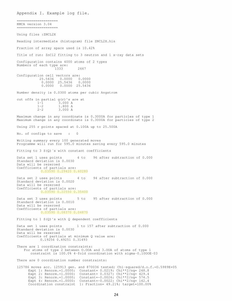
would run the RMCA program with files called cscl with various extensions. This name is given to anumber of files used by the program. The general program parameters are supplied in name.dat. The firsttime that the prograni is run there must be a file name.cfg containing the positions, or configuration, of theatoms. It is only necessary to calculate g(r) once at the beginning of the run, thereafter only the change ing(r) needs to be calculated. To facilitate this the histograms representing g(r), as well as a binaryrepresentation of the atomic coordinates, are written out to a file name.his when the program terminates;the new configuration is also written separately to name.cfg. On the next run the histograms and theatomic coordinates will be read from name.his, rather than from name.cfg, unless any parameters havebeen changed which require the histograms to be recalculated. Saved configurations will be written toname.sav and the output results will be written to name.out. Information on the status of the program iswritten to name.log. An example log file is shown in Appendix I.

10.2. The confguration file

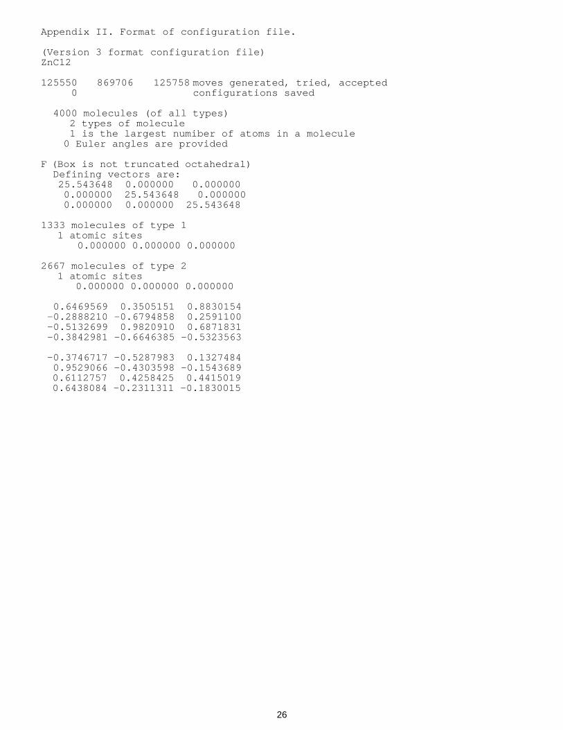
The configuration is normally cubic, but in general any parallelepiped can be used. If a crystalline systemis being modelled then obviously the box dimensions must be chosen to accomodate an integral number ofunit cells in each direction, with the numbers being chosen to make the dimensions as equal as possible. Theatomic coordinates are defined in terms of the box coordinates and are normalised to limits of ±1.0. The boxcoordinates are then defined in terms of the laboratory coordinates by the matrix given in the top of theconfiguration file. The values in this matrix are strictly only required to be relative; their absolute values arerecalculated from the density every time the program is run and these are then written into the newconfiguration file. However some programs for analysis of configurations do not check the density (and mayproduce erroneous results) so it is sensible to always use absolute values. For a cubic box the diagonal termsin the matrix are equal to half the box length (L/2) in Å.

The numbers of different types of atoms and the order of their coordinates are given in the top of theconfiguration file. The atomic coordinates then follow in a single list. The choice of a format in which thesystem is not explicitly identified in the configuration file (other than by the title) is made deliberately;configurations can then be easily modified or used as starting configurations for different systems with aminimal amount of editing. The same format of configuration file is also used for molecular systems, whereboth coordinates and Euler angles define the molecules. For this reason atoms are defined as molecules witha single atomic site. An example configuration file is shown in Appendix II.

10.3. The data file

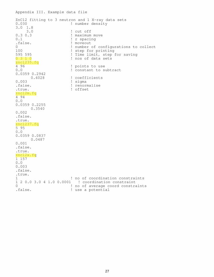
The RMCA data file name.dat can be thought of as being divided into various sections. Thedescription that follows is given section by section. An example data file is shown in Appendix III.

17

10. 3. 1. General parameters.

title character*80 A title for the run.rho real Number density of system in atoms Å-3.

rcut real array The closest allowed approach of two particles. There should be avalue for each partial g(r). There are thus n(n + 1)/2 values for an-component system. As in all other parts of the program thepartials are given in the order 1-1, 1-2, ..., 1-n, 2-2, ..., 2-n, ... n-n.See section 9.2 for a description of the use of this parameter.

delta real array The maximum move for each type of particle. Recommendedvalues are in the range 0.05-0.5. A value of zero is allowable, inwhich case the program will not attempt to move those particles.See section 9.3 for a description of the use of this parameter.

dr real The spacing for calculating g(r). See section 9.4 for a descriptionof the use of this parameter.

moveout logical This should be set .true. if, and only if, there are some particlesthat do not satisfy the cut-off restrictions and you want topreferentially choose these to be moved. 10% of the time one ofthese particles will be chosen, and 10% of the time any particlewill be chosen.

ncoll integer The number of configurations to collect after convergence. Theprogram will stop when ncoll configurations have beencollected.

iprint integer Determines how often a summary will be written to the standardoutput. It will be written after every iprint moves generated,except that this will only occur when a move is accepted.iprint should not be too small or otherwise time will be wastedin continually writing to the .log file and this will become verylarge.

timelim real The time the program should run for, in minutes.

timesav real The interval at which the results should be saved to the outputfiles (they are always saved when the program ends anyway). Ifthe program is left running for a very long time it is best to savethe results every now and then, perhaps once an hour. The resultsshould not be saved too often as this simply wastes time writinglarge files.

10.3.2. Parameters referring to all data sets.

nexpt integer array Four values, being the number of experimental data sets ofdifferent types. The first is the number of G(r) constraints, thesecond the number of S(Q)’s, the third the number of F(Q)’s, (forthe purpose of this program the difference between S(Q) and F(Q)

18

is that the former has constant coefficients of partial structurefactors whereas the latter has Q dependent coefficients as may bethe case with x-ray data), and the fourth the number of EXAFSdata sets. Definitions of these quantities in terms of partialstructure factors and radial distribution functions are given insection 9.7.

10.3.3. Parameters for each G(r) constraint.

file character*80 File containing the experimental data.nxl,nx2 integers The indices of the first and last data point to be used. If nx2 is

larger than the number of data points the last data point to be usedwill be the last data point given. If the r value corresponding tonx2 is larger than L/2 then nx2 will be reduced appropriately

c real A constant to be subtracted from the data on input.coeff real array The coefficients of each of the partial g(r)’s.sigma real The standard deviation to be used.renorm logical .true. if data renormalisation is required.

19

10.3.4. Parameters for each S(Q) constraint.

file character*80 File containing the experimental data.nx1,nx2 integers The indices of the first and last data points in the experimental

data file. If nx2 is larger than the number of data points the lastdata point used will be the last data point given.

c real A constant to be subtracted from the data on input.coeff real array The coefficients of each of the partial structure factors.sigma real The standard deviation to be used.renorm logical .true. if data renormalisation is required.offset logical .true. to subtract a constant from the data.

10.3.5. Parameters for each F(Q) constraint.

file character*80 File containing the experimental data and the coefficients of thepartial structure factors.

nx1,nx2 integers The indices of the first and last data point to be used. If nx2 islarger than the number of data points the last data point to be usedwill be the last data point given.

c real A constant to be subtracted from the data on input.sigma real The standard deviation to be used.renorm logical .true. if data renormalisation is required.offset logical .true. to subtract a constant from the data.

10.3.6. Parameters for afl EXAFS data (only present if there is some).

rmax real Maximum r value to be used.weight integer Data are to be weighted by Qweight. The experimental data should

be supplied unweighted, as weighting is done within the program.Data and fits written in the .out file will have the required Qweighting.

10.3.7. Parameters for each EXAFS constraint.

file character*80 File containing the experimental data.nx1,nx2 integers The indices of the first and last data point to be used. If nx2 is

larger than the number of data points the last data point to be usedwill be the last data point given. When EXAFS data is modelledtogether with diffraction data the values of nx1 and nx2 mustcorrespond to Q values which are a subset of the same Q values asin the data files for the diffraction data, and similarly in the file ofEXAFS coefficients, as the Q values will be taken from thediffraction, data files.

nx3,nx4 integers The indices of the first and last data points to be used in

calculation of c2 for the EXAFS data. nx3 and nx4 must liewithin the range of nx1 and nx2. These additional parameters aregiven for EXAFS data so that different ranges of the EXAFS data

20

can be modelled without having to recalculate the EXAFScoefficients.

edge integer Index number of the particle type corresponding to the absorptionedge being used.

file character*80 File containing the EXAFS coefficients.sigma real The standard deviation to be used.renorm logical .true. if data renormalisation is required. It is not

recommended that this option be used with EXAFS data sincerenormalisation by a negative number, corresponding to a phase

shift of p, may occur.offset logical .true. to subtract a constant from the data.

10.3.8. Parameters for coordination constraints.

ncoord integer The number of coordination constraints.

10.3.9. Parameters for each coordination constraint (one line per constraint).

typec integer The type of the central particle.typen integer The type of the neighbour particles.rcoord 2*real The two distances between which to calculate the coordination

number.coordno real The desired coordination number.coordfrac real The fraction of the central particles desired to have this

coordination number.sigmac real Effectively a parameter weighting this constraint relative to others

and the fit to the data.

10.3.10. Parameters for average coordination constraints..

ncoord integer The number of average coordination constraints.

10.3.11. Parameters for each average coordination constraint (one line per constraint)..

typec integer The type of the central particle.typen integer The type of the neighbour particles. Note that for the average

coordination number constraints, unlike the constraints oncoordination number distribution, there is no difference in theconstraint obtained by swapping neighbour and central particlesexcept in the value of coordination number required, as theconstraint is simply obtained by integration of gij(r) and gij(r) =gji(r).

rcoord 2*real The two distances between which to calculate the coordinationnumber.

coordno real The desired average coordination number.sigmac real Effectively a parameter weighting this constraint relative to others

and the fit to the data.

21

10.3.12. Parameters concerning a potential.

usepot logical .true. if using a potential. The remaining parameters in thissection are only present if we are.

temp real The absolute temperature.eunits real The energy units the potential is supplied in (in other words the

conversion factor to Joules).weight real The weighting factor for the potential. To use the program. for a

conventional Metropolis Monte Carlo simulation this should be 1.file character*80 The data file containing the potential tabulated at intervals of dr.

11. The experimental data files

The files containing the experimental data are in the DATA format as defined for the NDP series ofprograms. The number of points is given on the first line, the second line contains a title or otherinformation, and the subsequent lines contain the Q, S(Q) or r, G(r) values in two columns. An example fileis shown in Appendix III.

If the coefficients of the partial structure factors are to be included in the files, i.e. for F(Q) data asdefined in subsection 9.7, then they come after the F(Q) values in the order 11,12,...1n,22,23,...2n,...nn. ForX-ray data files in this format can be produced from files in the DATA format using the program XCOEFF.This has the option to normalise the form factors in three different ways, depending on how the original datahave been defined. An example file is shown in Appendix IV.

Note that if more than one set of diffraction data is supplied they must all be defined at the same Q, or r,points. You only need to use a subset of these points for fitting so it is possible to use data sets that coverdifferent ranges provided they are defined (for instance set to zero) at the points where data are not available.In the examples given in Appendix IV the second data set covers the range 0.3 to 15.9 at 157 points. Thefirst data set only covers the range 0.6 to 9.8, so it is defined to be zero at the other points. Points 4 to 96 areused for fitting to the first file (zncl235.fq in Appendix III) and points 1 to 157 for fitting to the second(zncl2x.fq in Appendix IV). The NDP program REBIN can be used to produce data sets satsifying thisrequirement.

If both EXAFS and diffraction data are supplied then the EXAFS data must be defined at a subset of thesame Q values as the diffraction data, since the Q values will be taken from the diffraction data files. It ispermitted to use only a subset of the values since there is no point in calculating the EXAFS coefficients at Qpoints where no data is available; this only makes the coefficient file larger. A subset of this subset can

actually be used for calculating c2, so the data fitted can be changed without recalculating the coefficient file.If only EXAFS data are supplied then the Q values are taken from this data file.

12. Other programs available

There are three other RMC codes available. RMCX fits to single crystal diffuse scattering data,RMCMuses semi-rigid molecules and RMCMAG models magnetic diffuse scattering. RMCPOW,for crystal structurerefinement based on powder diffraction data (Bragg scattering), is under development.

There are many programs available in the USEFUL suite for display and analysis of the results producedby RMCA, and for the creation and modification of configurations. Programs in the EXAFS suite can be usedfor preparing EXAFS data for RMC modelling. Some of the NDP suite of programs are convenient forpreparing experimental data sets in the correct format for input to RMCA. The MCGR program can be used

22

to create G(r) from a structure factor for initial RMC modelling. All of these programs are documentedseparately.

13. Installing the RMC programs

13.1. Source code

The program is written in a slightly extended Fortran-77 and compiles under VAX Fortran as well assome other versions of the language. Non-standard features used are names longer than 6 characters, use ofunderscore character, use of DO WHILE and DO ... ENDDO constructs. Most of the code is containedin one file. The configuration file reading and writing routines and some machine- dependent timing routinesare found in two other files.

The configuration of atoms is stored in a file with a standard format suitable for systems containing anynumber of components and for molecular systems. As this file will need to be read by analysis programs it isconvenient to keep the subroutines for reading and writing it separate from the main program. So that theidentical code for the main program can be used on any of the machines on which we wish to run it all themachine dependent parts are contained in separate subroutines. A random number generator must besupplied. In VAX Fortran the function ran(seed) generates a random number in the interval 0 to 1. Otherversions of Fortran may have equivalents. If not code for such a function is included.

The program is written to be general purpose and allocate array space when it runs. The total array spaceavailable is specified by a parameter statement near the beginning of the code and this may need to bechanged according to the computer system being used.

13.2. Compiling and running the program

The code is contained in the following files:

rmca.for - The main programrmc_cfg.for - The configuration reading and writing routinesrmc_vax.for - The machine dependent routines, VAX versionran.for - A random number generator (not needed for VAXes)

all of which should be compiled and linked (after any necessary alterations) in whatever manner isappropriate for your computing system. It is intended that the program be run in such a way that the data filename can be supplied on the command line. The Unix version of the machine dependent routines allows thiswith no further ado. On VAX/VMS systems it is necessary to define a symbol to run the program in thefollowing way:

rmca:== $user$disk:[user.rmc]rmca.exe

and then the program can be run by saying, for example

rmca ybco

13.3. Example files:

There are some example files available which demonstrate the use of the program and which can be usedfor testing. The example is molten copper. The configuration is small, only 250 atoms, partly so that the

23

program runs quickly and partly because larger files can be delayed during transfer by E-mail. The exampleconsists of the following files:

cu.dat - input datacusq.dat - experimental structure factorcu.cfg - configuration of 250 atomscuconv.cfg - converged configuration

The file cu.cfg contains a suitable starting configuration which can be used to run the program.Convergence is rapid for such a small configuration. An example configuration after convergence is incuconv.cfg. Note that the agreement with the experimental data is not exceptionally good atconvergence because of the small size of the configuration; this is because the oscillations in g(r) have notdied out by the largest distance at which g(r) can be calculated, i.e. half the box size. However this sufficesas a quick example. You will find that if you use a larger configuration (say 1000-2000 atoms) it is possibleto fit the experimental data very well indeed.

14. Using RMCA

RMCA is not a ’black box’ program. It will not tell you the ’correct’ structure of any material and it will notproduce wonderful results from poor data. What RMCA will do is allow you to explore, in a controlledmanner, what information on the three dimensional structure can actually be obtained from the experimentaldata provided. To do this it must be used in a sensible and thoughtful manner. The information obtainedmust also be used in an unbiased fashion. If the RMC model does not agree with a preferred theory then thisshould not simply be ignored. If RMC modelling produces significantly different structures that agree withthe same data then this is not a fault of the method, but rather it illustrates the inadequacy of the data. Thedifferent RMC models should then be used to predict whether different, or more accurate, experiments mightdistinguish between the model. In this way progress can be made.

24

Appendix I. Example log file.

====================RMCA version 3.04====================

Using files :ZNCL2X

Reading intermediate (histogram) file ZNCL2X.his

Fraction of array space used is 10.42%

Title of run: ZnCl2 fitting to 3 neutron and 1 x-ray data sets

Configuration contains 4000 atoms of 2 typesNumbers of each type are:

1333 2667

Configuration cell vectors are: 25.5436 0.0000 0.0000 0.0000 25.5436 0.0000 0.0000 0.0000 25.5436

Number density is 0.0300 atoms per cubic Angstrom

cut offs in partial g(r)’s are at1-1 3.000 A1-2 1.800 A2-2 3.000 A

Maximum change in any coordinate is 0.3000A for particles of type 1Maximum change in any coordinate is 0.3000A for particles of type 2

Using 255 r points spaced at 0.100A up to 25.500A

No. of configs to save : 0

Writing summary every 100 generated movesProgramme will run for 595.0 minutes saving every 595.0 minutes

Fitting to 3 S(Q)´s with constant coefficients

Data set 1 uses points 4 to 96 after subtraction of 0.000Standard deviation is 0.0030Data will be rezeroedCoefficients of partials are:

0.03590 0.29420 0.60280

Data set 2 uses points 4 to 94 after subtraction of 0.000Standard deviation is 0.0020Data will be rezeroedCoefficients of partials are:

0.03590 0.22550 0.35400

Data set 3 uses points 5 to 95 after subtraction of 0.000Standard deviation is 0.0010Data will be rezeroedCoefficients of partials are:

0.03590 0.08370 0.04870

Fitting to 1 S(Q)'s with Q dependent coefficients

Data set 1 uses points 1 to 157 after subtraction of 0.000Standard deviation is 0.0030Data will be rezeroedCoefficients of partials at minimum Q value are:

0.19256 0.49251 0.31493

There are 1 coordination constraints:For atoms of type 2 between O.OOA and 3.OOA of atoms of type 1

constraint is 100.0% 4-fold coordination with sigma-0.10OOE-03

There are 0 coordination number constraints:

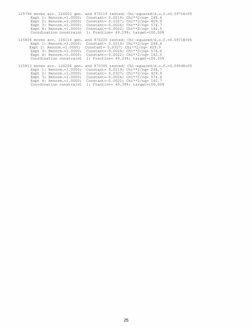
125786 moves acc. 125913 gen. and 870036 tested; Chi-squared/d.o.f.=O.5989E+05Expt 1: Renorm.=1.0000; Constant= 0.0219; Chi**2/nq= 248.8Expt 2: Renorm.=1.0000; Constant= 0.0327; Chi**2/nq= 429.4Expt 3: Renorm.=1.0000; Constant=-0.0026; Chi**2/nq= 574.5Expt 4: Renorm.=1.0000; Constant=-0.0022; Chi**2/nq= 142.4Coordination constraint 1: Fraction= 49.21%; target=100.00%

25

125796 moves acc. 126003 gen. and 870119 tested; Chi-squared/d.o.f.=O.5971E+05Expt 1: Renorm.=1.0000; Constant= 0.0219; Chi**2/nq= 248.6Expt 2: Renorm.=1.0000; Constant= 0.0327; Chi**2/nq= 429.9Expt 3: Renorm.=1.0000; Constant=-0.0026; Chi**2/nq= 574.7Expt 4: Renorm.=1.0000; Constant=-0.0022; Chi**2/nq= 142.5Coordination constraint 1: Fraction= 49.29%; target=100.00%

125806 moves acc. 126116 gen. and 870220 tested; Chi-squared/d.o.f.=0.5971E+05Expt 1: Renorm.=1.0000; Constant= 0.0219; Chi**2/nq= 248.6

Expt 2: Renorm.=l.0000; Constant= 0.0327; Chi**2/nq= 429.9Expt 3: Renorm.=1.0000; Constant=-0.0026; Chi**2/nq= 574.6Expt 4: Renorm.=1.0000; Constant=-0.0022; Chi**2/nq= 142.5Coordination constraint 1: Fraction= 49.29%; target=100.00%

125813 moves acc. 126206 gen. and 870300 tested; Chi-squared/d.o.f.=O.5954E+05Expt 1: Renorm.=1.0000; Constant= 0.0219; Chi**2/nq= 248.7Expt 2: Renorm.=1.0000; Constant= 0.0327; Chi**2/nq= 429.9Expt 3: Renorm.=1.0000; Constant=-0.0026; Chi**2/nq= 574.6Expt 4: Renorm.=1.0000; Constant=-0.0022; Chi**2/nq= 142.7Coordination constraint 1: Fraction= 49.36%; target=100.00%

26

Appendix II. Format of configuration file.

(Version 3 format configuration file)ZnC12

125550 869706 125758 moves generated, tried, accepted 0 configurations saved

4000 molecules (of all types) 2 types of molecule 1 is the largest numiber of atoms in a molecule 0 Euler angles are provided

F (Box is not truncated octahedral) Defining vectors are:

25.543648 0.000000 0.0000000.000000 25.543648 0.0000000.000000 0.000000 25.543648

1333 molecules of type 11 atomic sites

0.000000 0.000000 0.000000

2667 molecules of type 21 atomic sites 0.000000 0.000000 0.000000

0.6469569 0.3505151 0.8830154-0.2888210 -0.6794858 0.2591100-0.5132699 0.9820910 0.6871831-0.3842981 -0.6646385 -0.5323563

-0.3746717 -0.5287983 0.1327484 0.9529066 -0.4303598 -0.1543689 0.6112757 0.4258425 0.4415019 0.6438084 -0.2311311 -0.1830015

27

Appendix III. Example data file

ZnC12 fitting to 3 neutron and 1 X-ray data sets0.030 ! number density3.0 1.8

3.0 ! cut off0.3 0.3 ! maximum move0.1 ! r spacing.false. ! moveout0 ! number of configurations to collect100 ! step for printing595 595 ! Time limit, step for saving0 3 1 0 ! nos of data setszncl235.fq4 96 ! points to use0.0 ! constant to subtract0.0359 0.2942

0.6028 ! coefficients0.003 ! sigma.false. ! renormalise.true. ! offsetzncl2m.fq4 940.00.0359 0.2255

0.35400.002.false..true.zncl237.fq5 950.00.0359 0.0837

0.04870.001.false..true.zncl2x.fq1 1570.00.003.false..true.1 ! no of coordination constraints1 2 0.0 3.0 4 1.0 0.0001 ! coordination constraint0 ! no of average coord constraints.false. ! use a potential

28

Appendix IV. Format of experimental data files.

(a) S(Q) file

157ZnCl(35)2 neutron data

0.3000000 0.0000000E+000.4000000 0.0000000E+000.5000000 0.0000000E+000.6000000 -0.81164380.7000000 -0.76340960.8000000 -0.70734780.9000000 -0.5942892 . . .9.500000 -6.0869232E-029.600000 -3.5594340E-029.700001 -3.7083361E-029.800000 -6.2068522E-029.900001 0.0000000E+0010.00000 0.0000000E+0010.10000 0.0000000E+00 . . .15.60000 0.0000000E+0015.70000 0.0000000E+0015.80000 0.0000000E+0015.90000 0.0000000E+00

(b) F(Q) file

157ZnC12 X-ray data0.3000000 -0.7132038 0.1925575 0.4925125 0.31493010.4000000 -0.6189207 0.1936396 0.4928108 0.31354970.5000000 -0.6391176 0.1950143 0.4931799 0.31180580.6000000 -0.6021546 0.1966695 0.4936098 0.30972080.7000000 -0.5377059 0.1985902 0.4940888 0.30732110.8000000 -0.4991220 0.2007589 0.4946047 0.30463630.9000000 -0.4558854 0.2031563 0.4951446 0.3016990 . . .15.60000 -3.1411961E-02 0.2695458 0.4992644 0.231189815.70000 -3.8649879E-02 0.2710147 0.4991521 0.229833315.80000 -3.9273359E-02 0.2724817 0.4990322 0.228486115.90000 -3.6237735E-02 0.2739459 0.4989051 0.2271491

29

RMC bibliography.

1 N. Metropolis, A.W. Rosenbluth, M.N. Rosenbluth, A.H. Teller and E. TellerJ. Phys. Chem. 21 1087

2 Atomic arrangement in vitreous selenium. R. Kaplow, T.A. Rowe and B.L. Averbach.1968 Phys. Rev. 168 1068

3 Monte Carlo models of atomic arrangements in arsenic-selenium glass. A.L. Renninger, M.D. Rechtin andB.L. Averbach. 1974 J. Non-Cryst. Solids 16 1

4 Reverse Monte Carlo simulation: a new technique for the determination of disordered structures. R LMcGreevy and L Pusztai. 1988 Mol. Simulation. 1 359-367

5 The structure of molten LiCl. R L McGreevy and M A Howe.1989 J. Phys: Condensed Matter 1 9957-62

6 The structure of liquid copper selenide. M.A. Howe.1989 Physica B160 170

7 Structure modelling of Molecular liquids for the systems Benzene, Hexafluorobenzene and theirequimolar mixture. M. Ostheimer and H. Bertagnolli. 1989.

Z. Phys. Chem. Neue Folge 162 1718 Reverse Monte Carlo simulation techniques for combining X-ray and neutron diffraction data. R L

McGreevy. 1989 IOP conference series 101 41-509 Orientational correlations in the liquid halogens. M.A. Howe.

1990 Mol. Phys. 69 16110 The hydration of ions in aqueous solution: reverse Monte Carlo analysis of neutron diffraction data. M.A.

Howe. 1990 J. Phys: Condensed Matter 2 24111 Comments on reverse Monte Carlo simulation. R.A. Evans.

1990 Mol. Sim. 4 40912 Structural disorder in AgBr at the approach to melting. D A Keen, R L McGreevy and W Hayes. 1990 J.

Phys: Condensed Matter 2 2773-278613 Structural disorder in AgBr: RMC analysis of powder neutron diffraction data. D A Keen, W Hayes, R L

McGreevy and K N Clausen. 1990 Phil. Mag. Lett. 61349-357

14 Structural modelling of glasses using reverse Monte Carlo simulation. D A Keen and R L McGreevy.1990 Nature 344 423-42

15 The structures of molten salts. R L McGreevy and L Pusztai.1990 Proc. Roy. Soc. A 430 241-261

16 The structure of glassy Zinc Chloride: A reverse Monte Carlo study. L Pusztai and R L McGreevy. 1990J. Non-Cryst. Solids 117-118 627-628

17 Reverse Monte Carlo simulation for the analysis of EXAFS data. S J Gurman and R L McGreevy 1990 J.Phys: Condensed Matter 2 9463-9474

18 Reverse Monte Carlo (RMC) simulation: modelling structural disorder in crystals, glasses and liquidsfrom diffraction data. R L McGreevy, M A Howe, D A Keen and K N Clausen. 1990 IOPconference series 107 165-184

19 The structure of molten K-Pb, Rb-Pb and Cs-Pb alloys. M A Howe and R L McGreevy. 1991 J. Phys:Condensed Matter 3 577-591

20 The metal-non metal transition in expanded caesium. V M Nield, M A Howe and R L McGreevy. 1991 J.Phys: Condensed Matter 3 7519-7525

21 Determination of three body correlations in liquids by RMC modelling of diffraction data. I. Theoreticaltests. M A Howe and R L McGreevy. 1991 Phys. Chem. Liq. 24 1-12

22 Determination of disordered magnetic structures by RMC modelling of neutron diffraction data. D AKeen and R L McGreevy. 1991 J. Phys: Condensed Matter 3 7383- 7394

23 The structure of liquid "He across the A-point. L Pusztai and R L McGreevy. 1991

30

Phys. Chem. Liq. 24 119-12524 The structure of a-C:H by neutron and X-ray scattering. R.J. Newport, P.J.R. Honeybone, S.P. Cottrell, J.

Franks, P. Revell, R.J. Cernik and W.S. Howells. 1991 Surf. Coat. and Tech. 47 60825 Fractal aspects of superionic glasses from Reverse Monte Carlo simulations. L Börjesson, R L McGreevy

and W S Howells. 1992 Phil. Mag. B 65 261-27126 Neutron scattering studies of disorder and melting in Ag and Cu halides. D A Keen, V M Nield, R L

McGreevy and W Hayes. 1992 Physica B 180-181 798-80127 Determining the structures of disordered materials by diffuse neutron scattering and RMC modelling. R L

McGreevy, M A Howe, V M Nield, J D Wicks and D A Keen. 1992 Physica, B 180-181 801-80428 RMC: modelling disordered structures. R L McGreevy and M A Howe. 1992

Annual Review of Materials Science 22 217-24229 Structural disorder in AgBr at the approach to melting. IL V M Nield, D A Keen, W Hayes and R L

McGreevy. 1992 J. Phys: Condensed Matter 4 6703-671430 The structure of the C70 molecule. D.R. McKenzie, C.A. Davis, D.J.H. Cockayne, D.A. Muller and A.M.

Vassallo. 1992 Nature 355 62231 The structure of superionic glasses from neutron diffraction and reverse Monte Carlo modelling. L.

Börjesson, R.L. McGreevy and J.D. Wicks. 1992 J. de Phys. IV C2 10732 Determination of three body correlations in liquids by RMC modelling of diffraction data. IL Elemental

liquids. M A Howe, R L McGreevy, L Pusztai and I Borzsak. 1993 Phys. Chem. Liq. 25 20433 RMC techniques for structural modelling. R L McGreevy.

1993 Adv. Solid State Chem. in press34 Neutron diffraction and RMC modelling: complementary techniques for the determination of disordered

structures. R L McGreevy. 1993 Int. J. Mod. Phys. B 7 296535 RMC: fact and fiction. R.L. McGreevy.

1993 J. Non-Czyst. Solids 156-158 94936 The determination of the structure of (AgI)x(AgPO3)1-x glass by a combination of X-ray and neutron

diffraction data. J.D. Wicks, R.L. McGreevy and L. Börjesson. 1993 Int. J. Mod. Phys. B in press37 RMC techniques for the determination of partial structure factors. R.L. McGreevy. 1993 Int. J. Mod.

Phys. B in press38 A reverse Monte Carlo study of amorphous Ti67Ni33. E.W. Iparraguirre, J. Sietsma and B.J. Thijsse. 1993

J. Non-Cryst. Solids 156-158 96939 The performance of the Reverse Monte Carlo method applied to the metallic glasses Ni81B19 and Ti67Ni33.

E.W. Iparraguirre, J. Sietsma and B.J. Thijsse. 1993 Int. J. Mod. Phys. B in press40 A reverse Monte Carlo study of amorphous Ni81B19. E.W. Iparraguirre, J. Sietsma and B.J. Thijsse. 1993

Comp. Phys. Comm. in press41 C. Back, J.M. Dubois and R. Bellissent. RMC simulation of a metallic glass.

1993 Int. J. Mod. Phys. B in press42 RMC modelling of the structure of liquid lithium-silicon alloys.

P.H.K. de Jong, P. Verkerk and L.A. de Graaf. 1993 Int. J. Mod. Phys. B in press43 The structure of liquid lithium-silicon alloys. P.H.K. de Jong, P.Verkerk. W. van der Lugt, W.S. Howells

and L.A. P. de Jong 1993 J. Non-Cryst. Solids 156-158 97844 RMC experimentation on a metal-meta-I amorphous alloy. M. Bionducci. F. Buffa, G. Licheri and G.

Navarra. 1993 Int. J. Mod. Phys. B in press45 Amorphous CuZr alloy investigated by anomalous X-ray scattering. M. Bionducci, F. Buffa, G. Licheri

and G. Navarra. 1993 Int. J. Mod. Phys. B in press46 Structure study of Ni62Nb38 metallic glass using reverse Monte Carlo simulation. L. Pusztai and E. Svib.

1993 J. Non-Czyst. Solids 156-158 97347 A complete atomistic model of molten poly(ethylene) from neutron scattering data: a new methodologyfor polymer structures. B. Rosi-Schwaxtz and G.R. Mitchell. 1993 submitted to Makromol. Chemie - Theoryand Simulation

31

The structure of liquid sulphur: an RMC case study

L Karlsson and R L McGreevy

October 1993

Introduction

The aim of this paper is to describe, in considerable detail, how the reverse Monte Carlo method and theRMCA (version 3) program (and related programs) can be applied to the results of a particular diffractionexperiment. Hopefully the reader will then understand how to apply the program(s) to their own data in alogical and efficient manner.

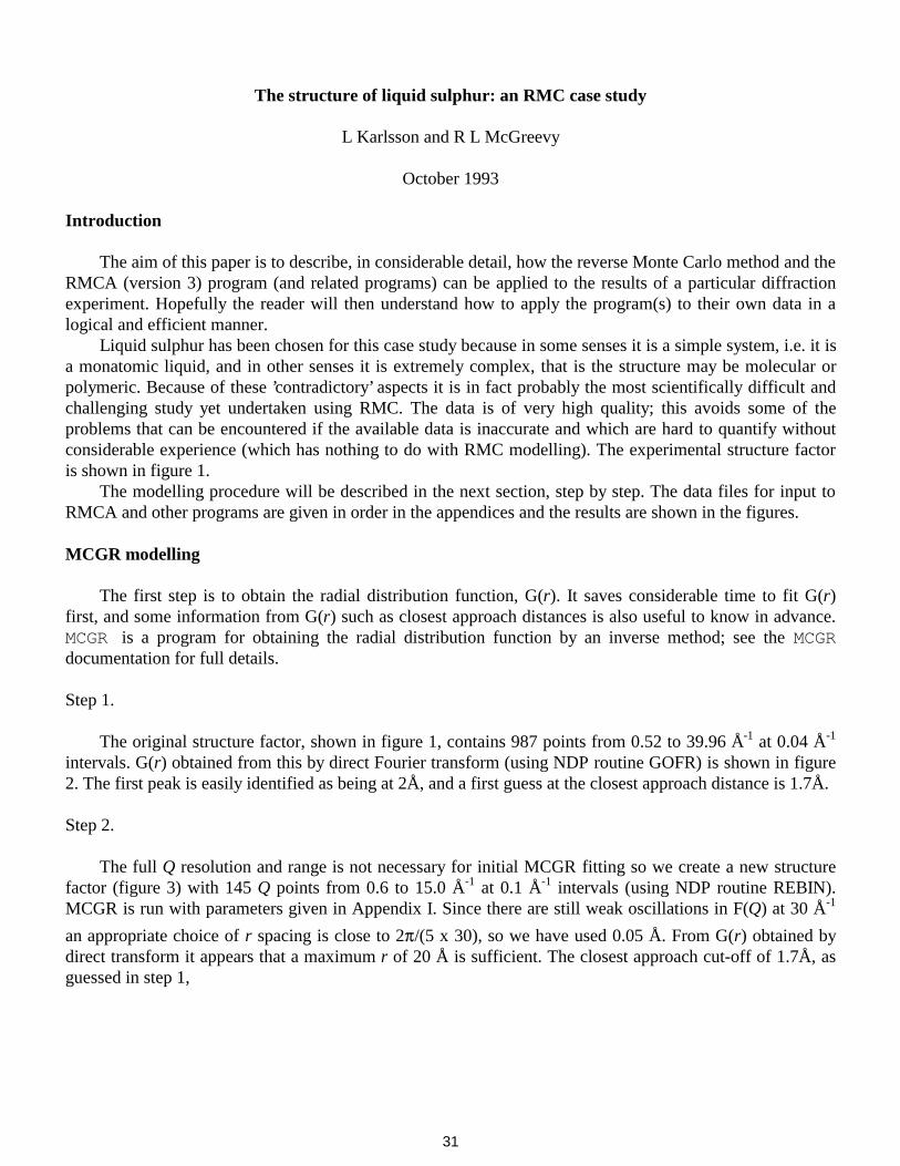
Liquid sulphur has been chosen for this case study because in some senses it is a simple system, i.e. it isa monatomic liquid, and in other senses it is extremely complex, that is the structure may be molecular orpolymeric. Because of these ’contradictory’ aspects it is in fact probably the most scientifically difficult andchallenging study yet undertaken using RMC. The data is of very high quality; this avoids some of theproblems that can be encountered if the available data is inaccurate and which are hard to quantify withoutconsiderable experience (which has nothing to do with RMC modelling). The experimental structure factoris shown in figure 1.

The modelling procedure will be described in the next section, step by step. The data files for input toRMCA and other programs are given in order in the appendices and the results are shown in the figures.

MCGR modelling

The first step is to obtain the radial distribution function, G(r). It saves considerable time to fit G(r)first, and some information from G(r) such as closest approach distances is also useful to know in advance.MCGR is a program for obtaining the radial distribution function by an inverse method; see the MCGRdocumentation for full details.

Step 1.

The original structure factor, shown in figure 1, contains 987 points from 0.52 to 39.96 Å-1 at 0.04 Å-1

intervals. G(r) obtained from this by direct Fourier transform (using NDP routine GOFR) is shown in figure2. The first peak is easily identified as being at 2Å, and a first guess at the closest approach distance is 1.7Å.

Step 2.

The full Q resolution and range is not necessary for initial MCGR fitting so we create a new structurefactor (figure 3) with 145 Q points from 0.6 to 15.0 Å-1 at 0.1 Å-1 intervals (using NDP routine REBIN).MCGR is run with parameters given in Appendix I. Since there are still weak oscillations in F(Q) at 30 Å-1

an appropriate choice of r spacing is close to 2p/(5 x 30), so we have used 0.05 Å. From G(r) obtained bydirect transform it appears that a maximum r of 20 Å is sufficient. The closest approach cut-off of 1.7Å, asguessed in step 1,

32

is used. The resulting fit to the structure factor is shown in figure 4 and the corresponding G(r) in figure 5.

The final c2 is 1.5. The G(r) suggests a new closest approach value of 1.9Å. The r spacing and maximum rused seem to be appropriate.

Step 3.

A new structure factor with 300 Q points from 0.6 to 30.5 Å-1 is created. MCGR is run again with acut-off of 1.9Å (parameters in Appendix II). The fit is shown in figure 6 and the resulting G(r) in figure 7.

The final c2 is 1.5. The first peak in G(r) is asymmetric so the cut-off used is probably too high.

Step 4.

Run MCGR again, this time with cut-off 1.85Å (Appendix III). The fit is shown in figure 8 and G(r) in

figure 9. The final c2 is 1.2. The first peak in G(r) is now more symmetric.

Step 5.

Now run MCGR with the same parameters, but saving 20 sets of G(r) to average over. The target c2 forsaving is 1.2 (Appendix IV). The resulting G(r) (average and standard deviation) is shown in figure 10. Thisaverage will initially be modelled by RMC.

RMC modelling (no constraints)

Step 6.

First the initial configuration must be created for the RMC model. Since the material studied is a liquid,and we are using no prior information (i.e. no constraints) the initial configuration chosen is random. Firstrun the program RMC:RANDOM (Appendix V) to create a random set of 4000 atomic positions. 4000atoms is typically found to be a reasonable number unless there are particular requirements for largerconfigurations.

Step 7.

To save time the random model should be made consistent with the atomic closest approach that isgoing to be used. This can be acheived most quickly, though not always completely if the packing fraction ishigh, using the program RMC:MOVEOUT. The best way to run this program is by moving the atoms apartin small steps. In this case we can start at 1.05Å and increase this to 1.85Å in 0.1Å steps, allowing 0.2Åmoves (see Appendix VI). G(r) for the resulting configuration (not the same as an equilibrated hard spheresimulation, though close) is shown in figure 11, in comparison to the target G(r) created by MCGR in step 5.

Step 8.

Now we run RMC, starting from the random configuration generated in step 7. The parameters are

given in Appendix VII The initial c2 is 1430. After 24 hours (VAX4000) it is 11.8. The fit is shown in figure

12.

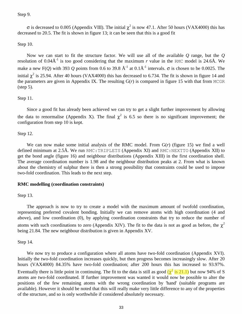
33

Step 9.

s is decreased to 0.005 (Appendix VIII). The initial c2 is now 47.1. After 50 hours (VAX4000) this hasdecreased to 20.5. The fit is shown in figure 13; it can be seen that this is a good fit

Step 10.

Now we can start to fit the structure factor. We will use all of the available Q range, but the Qresolution of 0.04Å-1 is too good considering that the maximum r value in the RMC model is 24.6Å. We

make a new F(Q) with 393 Q points from 0.6 to 39.8 Å-1 at 0.1Å-1 intervals. s is chosen to be 0.0025. The

initial c2 is 25.94. After 40 hours (VAX4000) this has decreased to 6.734. The fit is shown in figure 14 andthe parameters are given in Appendix IX. The resulting G(r) is compared in figure 15 with that from MCGR(step 5).

Step 11.

Since a good fit has already been achieved we can try to get a slight further improvement by allowing

the data to renormalise (Appendix X). The final c2 is 6.5 so there is no significant improvement; theconfiguration from step 10 is kept.

Step 12.

We can now make some initial analysis of the RMC model. From G(r) (figure 15) we find a welldefined minimum at 2.5Å. We run RMC:TRIPLETS (Appendix XI) and RMC:NEXTTO (Appendix XII) toget the bond angle (figure 16) and neighbour distributions (Appendix XIII) in the first coordination shell.The average coordination number is 1.98 and the neighbour distribution peaks at 2. From what is knownabout the chemistry of sulphur there is then a strong possibility that constraints could be used to imposetwo-fold coordination. This leads to the next step.

RMC modelling (coordination constraints)

Step 13.

The approach is now to try to create a model with the maximum amount of twofold coordination,representing preferred covalent bonding. Initially we can remove atoms with high coordination (4 andabove), and low coordination (0), by applying coordination constraints that try to reduce the number of

atoms with such coordinations to zero (Appendix XIV). The fit to the data is not as good as before, the c2

being 21.84. The new neighbour distribution is given in Appendix XV.

Step 14.

We now try to produce a configuration where all atoms have two-fold coordination (Appendix XVI).Initially the two-fold coordination increases quickly, but then progress becomes increasingly slow. After 20hours (VAX4000) 84.35% have two-fold coordination; after 200 hours this has increased to 93.97%.

Eventually there is little point in continuing. The fit to the data is still as good (c2 is 21.1) but now 94% of Satoms are two-fold coordinated. If further improvement was wanted it would now be possible to alter thepositions of the few remaining atoms with the wrong coordination by 'hand' (suitable programs areavailable). However it should be noted that this will really make very little difference to any of the propertiesof the structure, and so is only worthwhile if considered absolutely necessary.

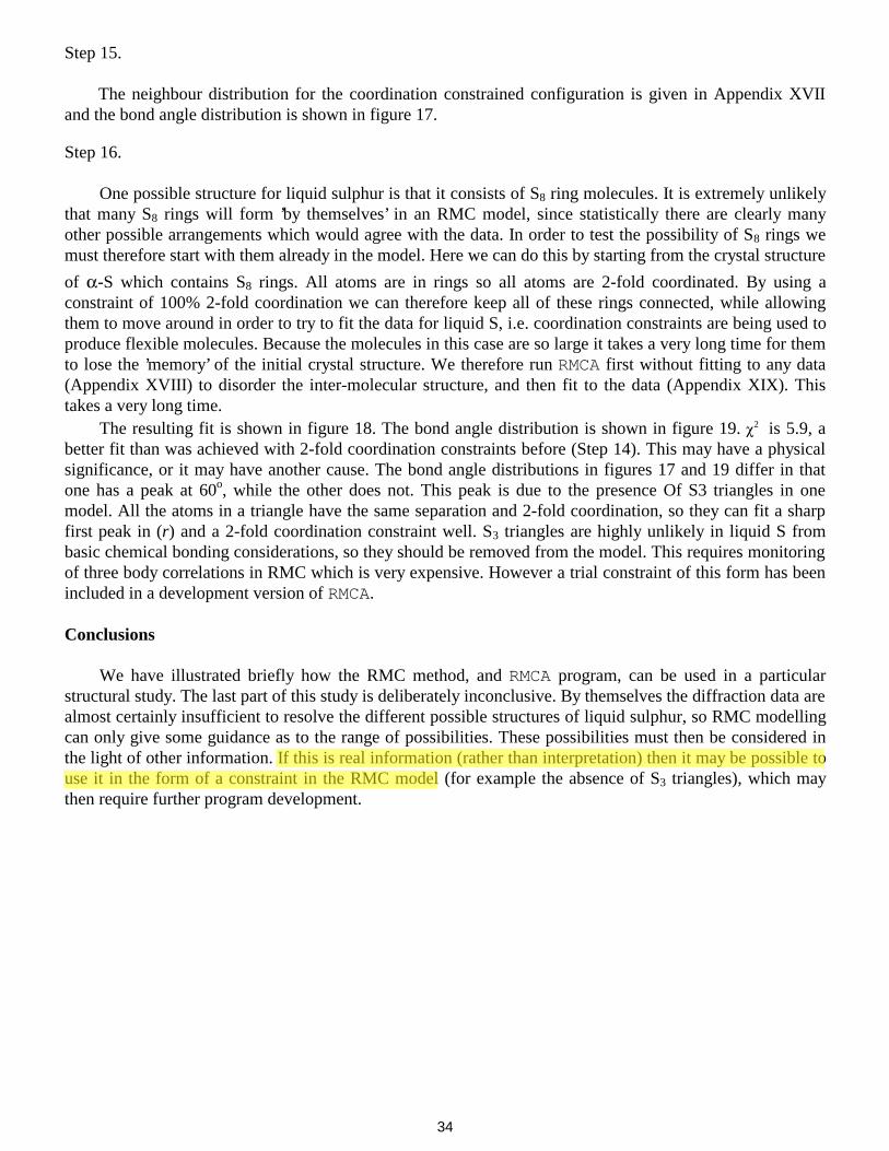
34

Step 15.

The neighbour distribution for the coordination constrained configuration is given in Appendix XVIIand the bond angle distribution is shown in figure 17.

Step 16.

One possible structure for liquid sulphur is that it consists of S8 ring molecules. It is extremely unlikelythat many S8 rings will form ’by themselves’ in an RMC model, since statistically there are clearly manyother possible arrangements which would agree with the data. In order to test the possibility of S8 rings wemust therefore start with them already in the model. Here we can do this by starting from the crystal structure

of a-S which contains S8 rings. All atoms are in rings so all atoms are 2-fold coordinated. By using aconstraint of 100% 2-fold coordination we can therefore keep all of these rings connected, while allowingthem to move around in order to try to fit the data for liquid S, i.e. coordination constraints are being used toproduce flexible molecules. Because the molecules in this case are so large it takes a very long time for themto lose the ’memory’ of the initial crystal structure. We therefore run RMCA first without fitting to any data(Appendix XVIII) to disorder the inter-molecular structure, and then fit to the data (Appendix XIX). Thistakes a very long time.

The resulting fit is shown in figure 18. The bond angle distribution is shown in figure 19. c2 is 5.9, abetter fit than was achieved with 2-fold coordination constraints before (Step 14). This may have a physicalsignificance, or it may have another cause. The bond angle distributions in figures 17 and 19 differ in thatone has a peak at 60o, while the other does not. This peak is due to the presence Of S3 triangles in onemodel. All the atoms in a triangle have the same separation and 2-fold coordination, so they can fit a sharpfirst peak in (r) and a 2-fold coordination constraint well. S3 triangles are highly unlikely in liquid S frombasic chemical bonding considerations, so they should be removed from the model. This requires monitoringof three body correlations in RMC which is very expensive. However a trial constraint of this form has beenincluded in a development version of RMCA.

Conclusions

We have illustrated briefly how the RMC method, and RMCA program, can be used in a particularstructural study. The last part of this study is deliberately inconclusive. By themselves the diffraction data arealmost certainly insufficient to resolve the different possible structures of liquid sulphur, so RMC modellingcan only give some guidance as to the range of possibilities. These possibilities must then be considered inthe light of other information. If this is real information (rather than interpretation) then it may be possible touse it in the form of a constraint in the RMC model (for example the absence of S3 triangles), which maythen require further program development.

35

Figure 1. The experimental structure factor for liquid sulphur at 140oC.

Figure 2. G(r) obtained from the experimental structure factor by direct Fourier transform. (Step 1)

Figure 3. Rebinned structure factor used for inital MCGR fitting. (Step 2)

Figure 4. Initial MCGR fit (broken line) compared to the experimental data (solid line). (Step 2)

Figure 5. G(r) corresponding to the initial MCGR fit. (Step 2)

Figure 6. MCGR fit (broken line) to the experimental structure factor (solid line) with the G(r) cut-off at 1.9Å. (Step 3)

Figure 7. G(r) corresponding to the MCGR fit with the cut-off at 1.9 Å. (Step 3)

Figure 8. Final MCGR fit (broken line) to the experimental structure factor (solid line) with the G(r) cut-offat 1.85 Å. (Step 4)

Figure 9. G(r) corresponding to the MCGR fit with the cut-off at 1.85 Å. (Step 4)

Figure 10. Average and standard deviation of G(r) from the final MCGR fit. (Step 5)

Figure 11. G(r) for the initial random RMC configuration (solid line) compared to the MCGR result (brokenline). (Step 7)

Figure 12. Initial RMC fit (broken line) to the G(r) from MCGR (solid line). (Step 8)

Figure 13. Final RMC fit (broken line) to the G(r) from MCGR (solid line). (Step 9)

Figure 14. Final RMC fit (broken line) to the experimental structure factor (solid line), with no coordinationconstraints. (Step 10)

Figure 15. G(r) from the RMC model with no coordination constraints (solid line) compared to the MCGRresult (broken line). (Step 10)

Figure 16. Bond angle distribution for the RMC model with no coordination constraints. (Step 12)

Figure 17. Bond angle distribution for the RMC model with 2-fold coordination constraint. (Step 15)

Figure 18. RMC fit (broken line) to the experimental structure factor (solid line) for a flexible S8 ringmolecule model. (Step 16)

Figure 19. Bond angle distribution for the RMC model with flexible S8 ring molecules. (Step 16)

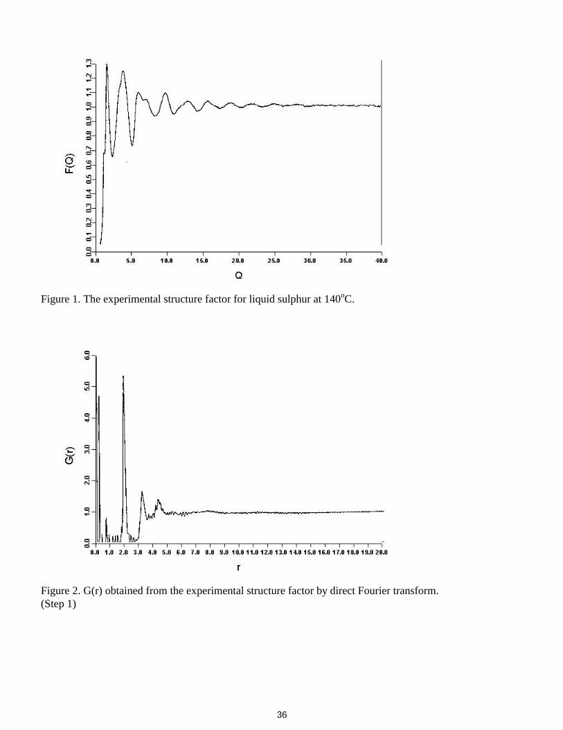
36

Figure 1. The experimental structure factor for liquid sulphur at 140oC.

Figure 2. G(r) obtained from the experimental structure factor by direct Fourier transform.(Step 1)

37

Figure 3. Rebinned structure factor used for initial MCGR fitting. (Step 2)

Figure 4. Initial MCGR fit (broken line) compared to the experimental data (solid line). (Step 2)

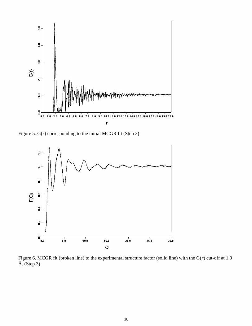
38

Figure 5. G(r) corresponding to the initial MCGR fit (Step 2)

Figure 6. MCGR fit (broken line) to the experimental structure factor (solid line) with the G(r) cut-off at 1.9Å. (Step 3)

39

Figure 7. G(r) corresponding to the MCGR fit with the cut-off at 1.9 Å. (Step 3)

Figure 8. Final MCGR fit (broken line) to the experimental structure factor (solid line) with the G(r) cut-offat 1.85 Å. (Step 4)

40

Figure 9. G(r) corresponding to the MCGR fit with the cut-off at 1.85Å. (Step 4)

Figure 10. Average and standard deviation of G(r) from the final MCGR fit (Step 5)

41

Figure 11. G(r) for the initial random RMC configuration (solid line) compared to the MCGR result (brokenline). (Step 7)

Figure 12. Initial RMC fit (broken line) to the G(r) from MCGR (solid line). (Step 8)

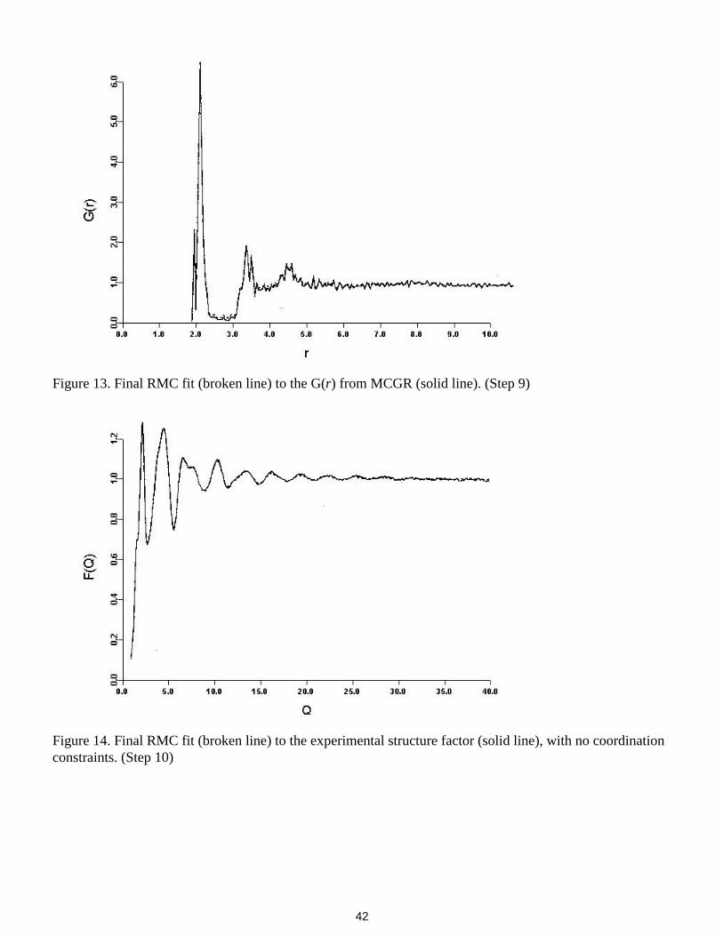
42

Figure 13. Final RMC fit (broken line) to the G(r) from MCGR (solid line). (Step 9)

Figure 14. Final RMC fit (broken line) to the experimental structure factor (solid line), with no coordinationconstraints. (Step 10)

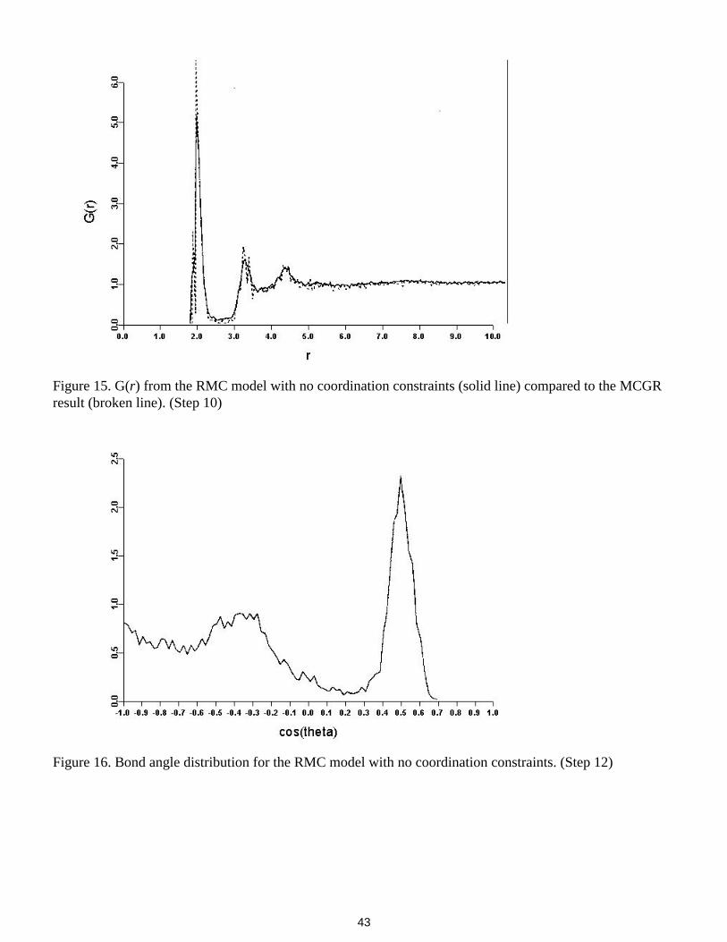
43

Figure 15. G(r) from the RMC model with no coordination constraints (solid line) compared to the MCGRresult (broken line). (Step 10)

Figure 16. Bond angle distribution for the RMC model with no coordination constraints. (Step 12)

44

Figure 17. Bond angle distribution for the RMC model with 2-fold coordination constraint. (Step 15)

Figure 18. RMC fit (broken line) to the experimental structure factor (solid line) for a flexible S8 ringmolecule model. (Step 16)

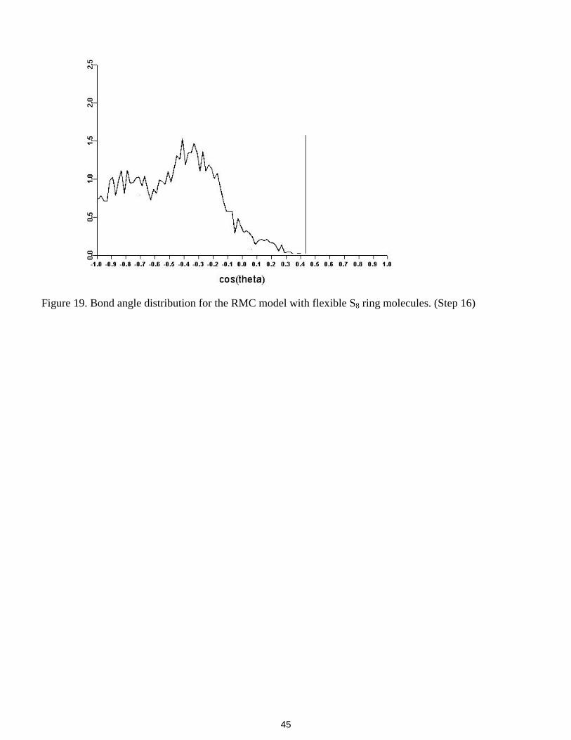
45

Figure 19. Bond angle distribution for the RMC model with flexible S8 ring molecules. (Step 16)

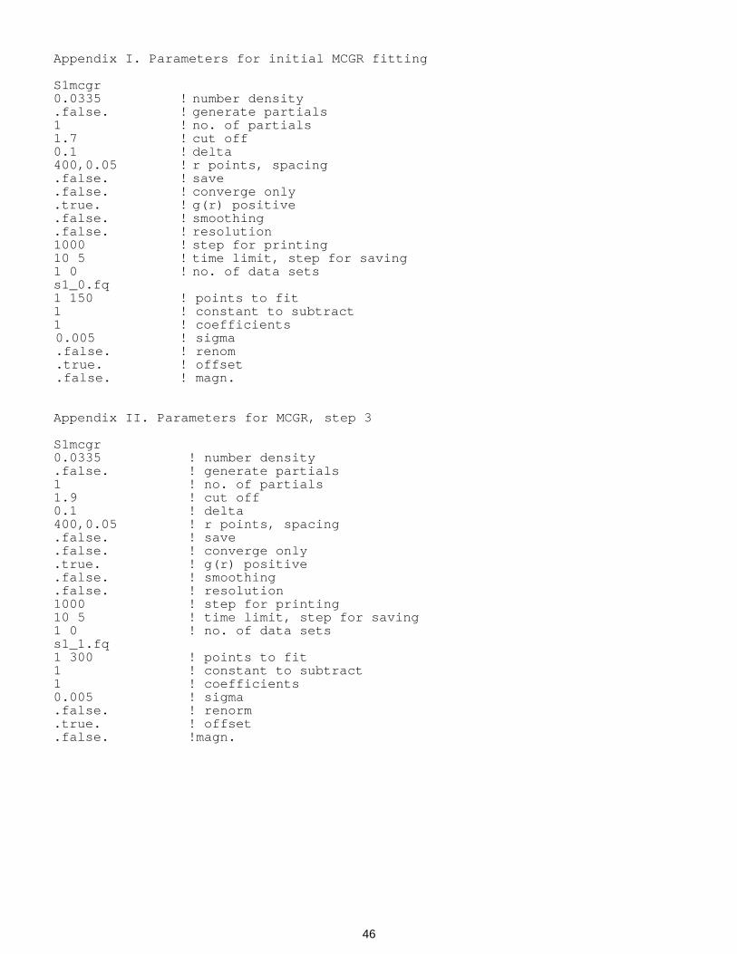
46

Appendix I. Parameters for initial MCGR fitting

S1mcgr0.0335.false.11.70.1400,0.05.false..false..true..false..false.100010 51 0s1_0.fq1 150110.005.false..true..false.

! number density! generate partials! no. of partials! cut off! delta! r points, spacing! save! converge only! g(r) positive! smoothing! resolution! step for printing! time limit, step for saving! no. of data sets

! points to fit! constant to subtract! coefficients! sigma! renom! offset! magn.

Appendix II. Parameters for MCGR, step 3

S1mcgr0.0335.false.11.90.1400,0.05.false..false..true..false..false.100010 51 0s1_1.fq1 300110.005.false..true..false.

! number density! generate partials! no. of partials! cut off! delta! r points, spacing! save! converge only! g(r) positive! smoothing! resolution! step for printing! time limit, step for saving! no. of data sets

! points to fit! constant to subtract! coefficients! sigma! renorm! offset!magn.

47

Appendix III. Parameters for MCGR, step 4

S1mcgr0.0335.false.11.850.1400,0.05.false..false..true..false..false.100020 101 0s1_1.fq1 300110.005.false..true..false.

! number density! generate partials! no. of partials! cut off! delta! r points, spacing! save! converge only! g(r) positive! smoothing! resolution! step for printing! time limit, step for saving! no. of data sets

! points to fit! constant to subtract! coefficients! sigma! renom! offset! magn.

Appendix IV. Parameters for final MCGR run, saving 20 sets of G(r)

S1mcgr0.0335.false.11.850.1400,0.05.true.1.2, 20.false..true..false..false.100060 101 0s1_1.fq1 300110.005.false..true..false.

! number density! generate partials! no. of partials! cut off! delta! r points, spacing! save

! converge only! g(r) positive! smoothing! resolution! step for printing! time limit, step for saving! no. of data sets

! points to fit! constant to subtract! coefficients! sigma! renorm! offset! magn.

48

Appendix V. A RMC:RANDOM run for creation of a random configuration

r rmc:randomTruncated octahedral ? (t/f) >fNumber of Euler angles >0Number of particle types >1Density >0.0335Number of particles of type 1>4000Output file >rand.cfgFORTRAN STOP

Appendix VII. Parameters for RMC, fitting G(r)

S10.0335 1.850.20.05.false.0100060 601 0 0 0slmcgr30.gr1 400010.01.false.00.false.

! number density! cut offs! maximum move! r spacing! whether to use moveout option! number of configurations to collect! step for printing! Time limit, step for saving! No. of g(r), neutron, X-ray, EXAFS expts

! Range of points! Constant to subtract! Coefficients! Standard deviation! Renormalise! no. of coordination constraints! no. of average coordination constraints! whether to use a potential

49

Appendix VI. A RMC:MOVEOUT run

r rmc:moveoutStarting configuration>rand.cfgClosest approaches >1.05592 atoms have too close neighbours

maximum move >1max. no. of iterations>1000591 atoms too crowded; 1 failed moves590 atoms too crowded; 1 failed moves589 atoms too crowded; 1 failed moves

. . .

2 atoms too crowded; 415 failed moves1 atoms too crowded; 416 failed moves0 atoms too crowded; 418 failed moves

Change cut-offs ? >tClosest approaches >1.15238 atoms have too close neighbours

Maximum move >0.2max. no. of iterations>1000 237 atoms too crowded; 1 failed moves 236 atoms too crowded; 4 failed moves . . . . .Change cut-offs ? >tClosest approaches >1.851533 atoms have too close neighboursMaximum move >0.2max. no. of iterations>60001532 atoms too crowded; 0 failed moves1531 atoms too crowded; 1 failed moves . . .

1 atoms too crowded; 5461 failed moves0 atoms too crowded; 5468 failed moves

Change cut-offs >fOutput file >moveout.cfgFORTRAN STOP

50

Appendix VIII. Parameters for RMC, fitting G(r) with decreased sigma

S10.0335 1.850.20.05.false.0100060 601 0 0 0s1mcgr30.gr1 400010.005.false.00.false.

! number density! cut offs! maximum move! r spacing! whether to use moveout option! number of configurations to collect! step for printing! Time limit, step for saving! No. of g(r), neutron, X-ray, EXAFS expts

! Range of points! Constant to subtract! Coefficients! Standard deviation! Renormalise! no. of coordination constraints! no. of average coordination constraints! whether to use a potential

Appendix IX. Parameters for RMC, fitting F(Q)

S10.03351.85

0.10.05.false.0100060 600 1 0 0S1_2.fq1 500010.0025.false..true.00.false.

! number density! cut offs! maximum move! r spacing! whether to use moveout option! number of configurations to collect! step for printing! Time limit, step for saving! No. of g(r), neutron, X-ray, EXAFS expts

! Range of points! Constant to subtract! Coefficients! Standard deviation! Renormalise! Offset! no. of coordination constraints! no. of average coordination constraints! whether to use a potential

51

Appendix X. RMC parameters, allowing data to renormalise

S10.03351.85

0.10.05.false.0100060 600 1 0 0s1_2.fq1 500010.0025.true..true.00.false.

! number density! cut offs! maximum move! r spacing! whether to use moveout option! number of configurations to collect! step for printing! Time limit, step for saving! No. of g(r), neutron, X-ray, EXAFS expts

! Range of points! Constant to subtract! Coefficients! Standard deviation! Renormalise! Offset! no. of coordination constraints! no. of average coordination constraints! whether to use a potential

Appendix XI. A RMC:TRIPLETS run, to get bond angle distribution

r rmc:tripletsNo. of theta pts >100No. of neighbours for bond ang (0 for all) >0Number of configurations >1Configuration file >S1_4.cfgMaximum r values >2.5Output file >s1.tripFORTRAN STOP

Appendix XII. A RMC:NEXTTO run, to get neighbour distribution

r rmc:nexttoConfiguration file >S1_4.cfgDistances from central particle >2.5Output fileS1.nexFORTRAN STOP

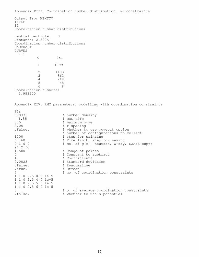
52

Appendix XIII. Coordination number distribution, no constraints

Output from NEXTTOTITLES1Coordination number distributions

central particle: 1Distance: 2.500ACoordination number distributionsBARCHARTCURVES7 1

0 251

1 1099

2 1483 3 863 4 248 5 48 6 8Coordination numbers:1.983500

Appendix XIV. RMC parameters, modelling with coordination constraints

S1r0.03351.85

0.50.05.false.0100060 600 1 0 0s1_2.fq1 500010.0025.false..true.41 1 0 2.5 0 0 le-51 1 0 2.5 4 0 le-51 1 0 2.5 5 0 le-51 1 0 2.5 6 0 le-50.false.

! number density! cut offs! maximum move! r spacing! whether to use moveout option! number of configurations to collect! step for printing! Time limit, step for saving! No. of g(r), neutron, X-ray, EXAFS expts

! Range of points! Constant to subtract! Coefficients! Standard deviation! Renormalise! Offset! no. of coordination constraints

!no. of average coordination constraints! whether to use a potential

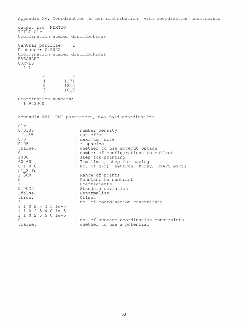
53

Appendix XV. Coordination number distribution, with coordination constraints

output from NEXTTOTITLE S1rCoordination number distributions

Central particle: 1Distance: 2.500ACoordination number distributionsBARCHARTCURVES4 1

0 01 11712 18103 1019

Coordination numbers:1.962000

Appendix XVI. RMC parameters, two-fold coordination

S1r0.03351.85

0.30.05.false.0100060 600 1 0 0s1_2.fq1 500010.0025.false..true.31 1 0 2.5 2 1 le-51 1 0 2.5 4 0 le-51 1 0 2.5 5 0 le-50.false.

! number density! cut offs! maximum. move! r spacing! whether to use moveout option! number of configurations to collect! step for printing! Tim limit, step for saving! No. of g(r), neutron, X-ray, EXAFS expts

! Range of points! Constant to subtract! Coefficients! Standard deviation! Renormalise! Offset! no. of coordination constraints

! no. of average coordination constraints! whether to use a potential

54

Appendix XVII. Coordination number distribution, two-fold coordination

output from NEXTTOTITLEs1rCoordination number distributions

Central particle: 1Distance: 2.500ACoordination number distributionsBARCHARTCURVES6 1

0 39 1 126 2 3759 3 38 4 36 5 2Coordination numbers:1.978000

Appendix XVIII. RMC parameters, to disorder the ring molecules

s1ring0.03351.85

0.30.05.false.0100060 600 0 0 011 1 0 2.5 2 1le-60.false.

! number density! cut offs! maximum move! r spacing! whether to use moveout option! number of configurations to collect! step for printing! Time limit, step for saving! No. of g(r), neutron, X-ray, EXAFS expts! no. of coordination constraints

! no. of average coordination constraints! whether to use a potential

55

Appendix XIX. RMC parameters, fitting data with ring molecule constraint

s1ring0.03351.85

0.30.05.false.0100060 600 1 0 0s1_2.fq1 500110.0025.false..true.11 1 0 2. 5 2 1 le-60.false.

! number density! cut offs! maximum move! r spacing! whether to use moveout option! number of configurations to collect! step for printing! Time limit, step for saving! No. of g(r), neutron, X-ray, EXAFS expts

! Range of points! Constant to subtract! Coefficients! Standard deviation! Renormalise! Offset! no. of coordination constraints

! no. of average coordination constraints! whether to use a potential