rmmc.eas.asu.edu j.-p. michel, p. somberg and j. silhan of overdetermined partial differential...
TRANSCRIPT

ROCKY MOUNTAINJOURNAL OF MATHEMATICSVolume 47, Number 2, 2017
PROLONGATION OF SYMMETRIC KILLINGTENSORS AND COMMUTING SYMMETRIES
OF THE LAPLACE OPERATOR
JEAN-PHILIPPE MICHEL, PETR SOMBERG AND JOSEF SILHAN
ABSTRACT. We determine the space of commuting sym-metries of the Laplace operator on pseudo-Riemannian man-ifolds of constant curvature and derive its algebra structure.Our construction is based on Riemannian tractor calculus,allowing us to construct a prolongation of the differentialsystem for symmetric Killing tensors. We also discuss someaspects of its relation to projective differential geometry.
1. Introduction. The Laplace operator is one of the cornerstonesof geometrical analysis on pseudo-Riemannian manifolds. There existsa close relationship between spectral properties of the Laplace oper-ator and local as well as global invariants of the underlying pseudo-Riemannian manifold.
The question of conformal symmetries of the Yamabe-Laplace oper-ator ∆Y on conformally flat spaces has been solved [8]. A differentialoperator D is a conformal symmetry of ∆Y , provided [∆Y , D] ∈ (∆Y ),where (∆Y ) is the left ideal generated by ∆Y in the algebra of differ-ential operators. These D operators are called conformal symmetriesbecause they preserve the kernel of ∆Y . On a given flat conformalmanifoldM , there is a bijection between the vector space of symmetricconformal Killing tensors and the quotient of the space of conformalsymmetries by (∆Y ). Note that the space of symmetric conformalKilling tensors is the solution space of a conformally invariant system
2010 AMS Mathematics subject classification. Primary 35J05, 35R01, 53A20,58J70.
Keywords and phrases. Killing tensors, prolongation of PDEs, commuting sym-metries of Laplace operator.
The first author was supported by the Belgian Interuniversity Attraction Pole(IAP) within the “Dynamics, Geometry and Statistical Physics” (DYGEST) frame-work. The second and third authors were supported by the grant agency of theCzech Republic, grant No. P201/12/G028.
Received by the editors on April 23, 2015.DOI:10.1216/RMJ-2017-47-2-587 Copyright c⃝2017 Rocky Mountain Mathematics Consortium
587

588 J.-P. MICHEL, P. SOMBERG AND J. SILHAN
of overdetermined partial differential equations, which is locally finite-dimensional.
In the present paper, we classify the commuting symmetries ofthe Laplace operator ∆ on pseudo-Riemannian manifolds of constantcurvature, i.e., manifolds locally isometric to a space form. In fact,the Laplace operator differs from the Yamabe-Laplace operator by amultiple of the identity operator; therefore, both operators share thesame commuting symmetries. The eigenspaces of the Laplace operatorare preserved by commuting symmetries, i.e., by linear differentialoperators D commuting with the Laplace operator:
[∆, D] = 0.
The vector space of commuting symmetries is generated by Killingvector fields and their far reaching generalization called symmetricKilling tensors, or Killing tensors for short. Their composition asdifferential operators provides an algebraic structure that we shalldetermine.
Killing 2-tensors on pseudo-Riemannian manifolds are the moststudied among Killing tensors, and they play a key role in the sep-aration of variables of the Laplace equation. The construction of com-muting symmetries out of Killing 2-tensors is well known in a numberof geometrical situations [7], particularly on constant curvature man-ifolds. Higher Killing tensors give integrals of motion for the geodesicequation and contribute to its integrability. They can be regardedas hidden symmetries of the underlying pseudo-Riemannian manifold.Killing tensors themselves are solutions of an invariant system of PDEs,and trace-free Killing tensors are special examples of conformal Killingtensors.
As a technical tool, we introduce, and to a certain extent develop, theRiemannian tractor calculus, focusing mainly on manifolds of constantcurvature. This allows a uniform description of the prolongation of theinvariant system of PDEs for Killing tensors and plays a key role inour analysis of the correspondence between commuting symmetries ofthe Laplace operator and Killing tensors. In particular, we obtain anexplicit version of the identification in [15], see also [17], of the space offixed valence Killing tensors with a representation of the general lineargroup.

PROLONGATION OF SYMMETRIC KILLING TENSORS 589
The Riemannian tractor calculus can be interpreted as the tractorcalculus for projective parabolic geometry in a scale correspondingto a metric connection in the projective class of affine connections.Restricting to locally flat special affine connections, Einstein metricconnections in the projective class correspond to manifolds of constantcurvature [11]. Since the Killing equations on symmetric tensor fieldsare projectively invariant [9], we may use invariant tractor calculusin projective parabolic geometry to construct commuting symmetries.Projective invariance explains that the space of Killing tensors carriesa representation of the general linear group.
As for the style of presentation and exposition, we have attemptedto make the paper accessible to a broad audience with basic knowledgein Riemannian geometry. Following this perspective, the structure ofour paper follows. After setting the conventions in Section 2, we intro-duce the rudiments of Riemannian tractor calculus in Section 3. Thecore of the article is in Section 4, where we construct the prolonga-tion of the differential system for Killing tensors and derive the spaceof differential operators preserving the spectrum of the Laplace opera-tor. Afterwards, we determine the underlying structure of associativealgebra on this space, induced by the composition of differential opera-tors. We compute explicit formulas for commuting symmetries of orderat most 3. In special cases, we compare commuting symmetries withconformal symmetries constructed in [8]. In Section 5, we interpretour results in terms of the holonomy reduction of a Cartan connectionin projective parabolic geometry and its restriction on a curved orbitequipped with an Einstein metric.
2. Notation and conventions. Let (M, g) be a smooth pseudo-Riemannian manifold. Throughout the paper, we employ Penrose’sabstract index notation and use Ea to denote the space of smoothsections of the tangent bundle TM on M , and Ea for the space ofsmooth sections of the cotangent bundle T ∗M . We also use E for thespace of smooth functions. All tensors considered are assumed to besmooth. With abuse of notation, we will often use the same symbolsfor the bundles and their spaces of sections. The metric gab will beused to identify TM with T ∗M . We shall assume that the manifold Mhas dimension n ≥ 2.

590 J.-P. MICHEL, P. SOMBERG AND J. SILHAN
An index which appears twice, once raised and once lowered, in-dicates the contraction. Square brackets [· · · ] will denote skew-symmetrization of enclosed indices, while round brackets (· · · ) will in-dicate symmetrization.
We set ∇ for the Levi-Civita connection corresponding to gab. Then,the Laplacian ∆ is given by
∆ = gab∇a∇b = ∇b∇b.
Since the Levi-Civita connection is torsion-free, the Riemannian cur-vature Rab
cd is given by
[∇a,∇b]vc = Rab
cdv
d,
where [·, ·] indicates the commutator bracket. The Riemannian curva-ture can be decomposed in terms of the totally trace-free Weyl curva-ture Cabcd, and the symmetric Schouten tensor Pab,
(2.1) Rabcd = Cabcd + 2gc[aPb]d + 2gd[bPa]c.
We will refer to Pab as a Riemannian Schouten tensor to distinguishfrom the projective Schouten tensor which will be introduced later inthis paper. We define J := Pa
a, such that
J =Sc
2(n− 1),
with Sc the scalar curvature.
Throughout the paper, we work (if not stated otherwise) on mani-folds of constant curvature, i.e., locally symmetric spaces with parallelcurvature
Rabcd =4
nJgc[agb] d,
cf., [18]. Thus, the function J is constant. In signature (p, q),M is thenlocally isomorphic to G/H, where G = SO(p+1, q) andH = SO(p, q) ifJ > 0, G = SO(p, q+1), H = SO(p−1, q+1) if J < 0, G = E(p, q) andH = SO(p, q) if J = 0. Here, we denote the group of pseudo-Euclideanmotions on Rp,q by E(p, q).
3. Tractor calculus in Riemannian geometry. The notion ofassociated tractor bundles is well known in the category of parabolicgeometries. We refer to [5] for a review with many applications. In

PROLONGATION OF SYMMETRIC KILLING TENSORS 591
this section, we introduce and develop rudiments of a class of tractorbundles in the category of pseudo-Riemannian manifolds, in closeanalogy with tractor calculi in parabolic geometries.
We assume M has constant curvature, i.e.,
Rabcd =4
nJgc[agb]d,
with J constant. We define the Riemannian standard tractor bundle orstandard tractor bundle, for short,
T := L ⊕ TM
where L denotes the trivial bundle over M .
The Levi-Civita connection ∇a induces a connection on T , which istrivial on L. The tractor connection is another connection on T , alsodenoted (with an abuse of notation) by ∇a, and defined by
∇a
(fµb
)=
(∇af − µa
∇aµb + 2
nJfδba
),(3.1)
where f ∈ E , µb ∈ Eb. In the first line, we use the isomorphismTM ∼= T ∗M . The dual connection on the dual bundle:
T ∗ := T ∗M ⊕ L,
also denoted by ∇a, is given by
∇a
(νbf
)=
(∇aνb + fgab∇af − 2
nJνa
),(3.2)
where νb ∈ Eb and f ∈ E . Direct computation shows that the curvatureof the tractor connection ∇ is trivial, i.e., the tractor connection ∇ isflat. Note that this connection differs from that induced by the Cartanconnection [5, subsection 1.5].
The bundle T is equipped with the symmetric bilinear form ⟨ , ⟩,
(3.3)⟨( f
µb
),
(fµ b
)⟩=
2
nJff + µb µb
which is invariant with respect to the tractor connection ∇. For J = 0,this form is non-degenerate and called the tractor metric. Then, ityields an isomorphism T ∼= T ∗.
592 J.-P. MICHEL, P. SOMBERG AND J. SILHAN
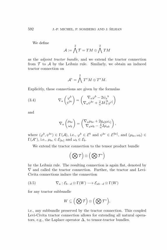
We define
A :=2∧T = TM ⊕
2∧TM
as the adjoint tractor bundle, and we extend the tractor connectionfrom T to A by the Leibniz rule. Similarly, we obtain an inducedtractor connection on
A∗ =2∧T ∗M ⊕ T ∗M.
Explicitly, these connections are given by the formulas
∇a
(φb
ψbc
)=
(∇aφ
b − 2ψab
∇aψbc + 2
nJδ[baφc]
)(3.4)
and
∇a
(µbc
ωb
)=
(∇aµbc + 2ga[bωc]
∇aωb − 4nJµab
),
where (φb, ψbc) ∈ Γ(A), i.e., φb ∈ Eb and ψbc ∈ E [bc], and (µbc, ωb) ∈Γ(A∗), i.e., µbc ∈ E[bc] and ωb ∈ Eb.
We extend the tractor connection to the tensor product bundle(⊗T)⊗(⊗
T ∗)
by the Leibniz rule. The resulting connection is again flat, denoted by∇ and called the tractor connection. Further, the tractor and Levi-Civita connections induce the connection
(3.5) ∇a : Eb···d ⊗ Γ(W ) −→ Eab···d ⊗ Γ(W )
for any tractor subbundle
W ⊆(⊗
T)⊗(⊗
T ∗),
i.e., any subbundle preserved by the tractor connection. This coupledLevi-Civita tractor connection allows for extending all natural opera-tors, e.g., the Laplace operator ∆, to tensor-tractor bundles.

PROLONGATION OF SYMMETRIC KILLING TENSORS 593
The invariant pairing on A induced by equation (3.3) is given by theformula
(3.6)⟨(φb
ψbc
),
(φ b
ψ bc
)⟩=
1
nJφaφa + ψabψab.
For J = 0, this defines a metric on A and A ∼= A∗. Moreover, there isa Lie algebra structure
[·, ·] : A⊗A −→ A,
given by
(3.7)
[(φb
ψbc
),
(φ b
ψ bc
)]=
(φrψ
ra − φrψra
−2ψr[bψrc] − 1
nJφ[bφc]
),
which is also invariant under the tractor connection.
Remark 3.1. Tractor connections can be defined on any Riemannianmanifold. For example, we can define ∇ on A by
∇a
(φb
ψbc
)=
(∇aφ
b − 2ψab
∇aψbc + 1
2Rbc
asφs
)for φb ∈ Eb and ψbc ∈ E [bc]. This definition originates in the work ofKostant [14]. We observe that, for a Killing vector field ka ∈ Ea, itsprolongation
(3.8) K =
(ka
12∇
[akb]
)∈ Γ(A)
is parallel for the tractor connection. Hence, any isometry is locallydetermined by its first jet.
We shall use abstract index notation for the adjoint tractor bundleas follows: Γ(T ) will be denoted by EA and Γ(A) will be denoted byEA where A = [A1A2]. Similarly, EA = Γ(A∗) and EA = Γ(A∗), thatis, we use boldface capital indices for an adjoint tractor bundle and itsdual.
There is a convenient way to treat the bundles T and T ∗, basedon the so-called injectors, or tensor-tractor frame, denoted by Y A, ZA
a

594 J.-P. MICHEL, P. SOMBERG AND J. SILHAN
for T and denoted by YA, ZaA for T ∗. These are defined by
(3.9)
(fµb
)= Y Af + ZA
b µb ,
(νbf
)= Zb
Aνb + YAf,
and their contractions are
Y AYA = 1, ZAa Z
bA = δ b
a and Y AZbA = ZA
a YA = 0.
The covariant derivatives in equations (3.1) and (3.2) are then encodedin covariant derivatives of these injectors:
∇cYA =
2
nJZA
a δac , ∇cZ
Aa = −Y Agac,
∇cZaA = − 2
nJYAδ
ac , ∇cYA = Za
Agca.
(3.10)
We denote tractor pairing equation (3.3) by hAB ∈ E(AB), which hasthe explicit form:
(3.11) hAB =2
nJYAYB + Za
AZbBgab.
Injectors for the adjoint tractor bundle EA are
YAa = Y [A1
ZA2]a and ZA
a = Z[A1
a1 ZA2]a2 ;
injectors for the dual bundle EA are
YaA = Y[A1Za
A2] and Z aA = Za1
[A1Z a2
A2],
that is,
(3.12)
(φb
ψa
)= φbYA
b + ψaZAa ,
(µa
ωb
)= µaZ a
A + ωbY bA,
where a = [a1a2]. The only nonzero contractions are
YAa Yb
A =1
2δ ba and ZA
aZ cA = δ c1
[a1 δ c2
a2].
The covariant derivatives (3.4) are then equivalent to
∇cYAb =
2J
nZAab δ
ac , ∇cZA
a = −2YA[a2ga1]c,
∇cZ aA = −4J
nY[a2
A δ a1]c , ∇cYb
A = ZabA gca,
(3.13)

PROLONGATION OF SYMMETRIC KILLING TENSORS 595
and the pairing (3.6) on EA can be written:
(3.14) hAB =4
nJYa
AYbBgab + Z a
AZbBga1b1ga2b2 .
A crucial component of our construction is the differential operator
(3.15) DA : Eb1···bs ⊗ Γ(W ) −→ Eb1···bs ⊗ Γ(A∗ ⊗W
)for a tractor subbundle
W ⊆(⊗
T)⊗(⊗
T ∗).
This operator is closely related to the so-called fundamental deriva-tive [5]. It is defined as follows: for f ∈ Γ(W ), we set
(3.16) DAf =
(0
2∇af
)∈ Γ(A∗ ⊗W ),
and, for φb ∈ Eb, we set
(3.17) DAφb =
(2gb[a1φa2]
2∇aφb
)∈ Eb ⊗ Γ(A∗).
Then, we extend DA to all tensor-tractor bundles by the Leibniz rule.Using injectors (3.12), formulas (3.16) and (3.17) are given by
DAf = 2YaA∇af,(3.18)
DAφb = 2YaA∇aφb + Z a
A2gb[a0φa1]
where a = [a1a2].
Theorem 3.2. Let M be a manifold of constant curvature. The oper-ator DA commutes with the coupled Levi-Civita tractor connection ∇c,
∇cDA = DA∇c : Eb1···bs ⊗ Γ(W ) −→ Ecb1···bsA ⊗ Γ(W ).
Proof. Since the tractor connection is flat, it is sufficient to provethe statement for W equal to the trivial line bundle. We present twoversions of the proof.
First, one can easily show by direct computation using equations(3.13) and (3.18) that the explicit formulas for the compositions ∇cDA
and DA∇c are the same when acting on f ∈ E and φb ∈ Eb. Hence, theformulas agree on any tensor bundle.

596 J.-P. MICHEL, P. SOMBERG AND J. SILHAN
Alternatively, recall that, for a Killing vector field ka ∈ Ea, itsprolongation KA ∈ Γ(A) is parallel, see equation (3.8). We furtherobserve that Lk = KADA is the Lie derivative along ka when acting ontensor bundles. Since Lk commutes with the covariant derivative, andthe space of Killing vector fields on manifolds with constant curvaturehas dimension equal to
dim(A) = n+1
2n(n− 1),
the statement follows. �
As a consequence of Theorem 3.2, DA also commutes with Laplaceoperator ∆ on functions, forms, etc. We will now make this result moregeneral and precise. Assume that
F : Γ(U1) −→ Γ(U2)
is a Riemannian invariant linear differential operator, acting betweentensor bundles U1 and U2. It can be written in terms of the metric,the Levi-Civita connection ∇ and the curvature J. Replacing ∇ in theformula for F by the coupled Levi-Civita tractor connection, we obtainthe operator
F∇ : Γ(U1 ⊗W ) −→ Γ(U2 ⊗W )
for any tractor subbundle
W ⊆(⊗
T)⊗(⊗
T ∗).
Note that, since the tractor connection is flat, the curvature of thecoupled Levi-Civita tractor connection agrees with the curvature ofthe Levi-Civita connection. Using Theorem 3.2 and ∇aJ = ∇ag = 0,we obtain the following.
Corollary 3.3. LetF : Γ(U1) −→ Γ(U2)
be a Riemannian invariant linear differential operator on the mani-fold M . Then, DA commutes with F∇, i.e.,
DA ◦ F∇ = F∇ ◦ DA : Γ(U1 ⊗W ) −→ Γ(U2 ⊗A∗ ⊗W ).

PROLONGATION OF SYMMETRIC KILLING TENSORS 597
4. Commuting symmetries of the Laplace operator.
Definition 4.1. Let U be a tensor bundle, and let
F : Γ(U) −→ Γ(U)
be a linear differential operator on M . A commuting symmetry ofoperator F is a linear differential operator D fulfilling DF = FD.
We are interested in commuting symmetries of the Laplace operatorF = ∆ on functions. They form a subalgebra of the associative algebraof linear differential operators acting on E . The exposition in the rest ofthis section closely follows that given in [8] for conformal symmetries.For a comparison of both types of symmetries, see Remark 4.16.
Let ℓ be a non-negative integer. A linear ℓth order differentialoperator acting on functions can be written:
(4.1) D = V a1···aℓ∇a1 · · ·∇aℓ+ LOTS,
where LOTS stands for lower order terms in D, and its principal symbolV a1···aℓ is symmetric in its indices V a1···aℓ = V (a1···aℓ).
Definition 4.2. A Killing tensor on M is a symmetric tensor fieldV a1···aℓ , fulfilling the first order differential equation
(4.2) ∇(a0V a1···aℓ) = 0.
The vector space of all Killing tensors of valence ℓ will be denotedby Kℓ.
Since differential equation (4.2) is overdetermined, the space Kℓ isfinite-dimensional. Note that the symmetric product of two Killingtensors is again a Killing tensor, such that
⊕ℓ≤0Kℓ is a commutative
graded algebra.
Theorem 4.3. Let D be an ℓth order commuting symmetry of theLaplace operator. Then, the principal symbol V a1···aℓ of D is a Killingtensor of valence ℓ.

598 J.-P. MICHEL, P. SOMBERG AND J. SILHAN
Proof. When D is of the form (4.1), we compute
(4.3) ∆D −D∆ = 2(∇bV a1···aℓ)∇b∇a1 · · ·∇aℓ+ LOTS,
and the claim follows. �
The converse of this statement is covered in the next theorem.
Theorem 4.4. There exists a linear map:
V a1···aℓ 7−→ DV ,
from symmetric tensor fields to differential operators, such that theprincipal symbol of DV is V a1···aℓ and DV ∆ = ∆DV if V is a Killingtensor.
The proof of Theorem 4.4 is postponed to the next section, wherethe Riemannian prolongation connection for symmetric powers of theadjoint tractor bundle is constructed. This allows explicit computationof the symmetry operators DV .
Combining both theorems, we deduce a linear bijection betweenthe space of Killing tensors and the space of commuting symmetriesof ∆. More explicitly, the space of 0th order commuting symmetries isthe space of constants, the space of first order commuting symmetriescontains in addition the Killing vector fields, and by induction, thespace of ℓth order commuting symmetries contains the space of (ℓ−1)thorder commuting symmetries together with a copy of the space Kℓ ofKilling tensors of valence ℓ. In particular, the dimension of the vectorspace of ℓth order symmetry operators is finite and equal to
dimK0 + dimK1 + · · ·+ dimKℓ.
4.1. Prolongation for Killing tensors. Let ka ∈ Ea be a Killingvector field. In Remark 3.1, we observed that its prolongation
K =(ka,
1
2∇[akb]
)∈ Γ(A)
is parallel for the tractor connection. Our aim is to construct analogousprolongation for Killing tensors.

PROLONGATION OF SYMMETRIC KILLING TENSORS 599
Lemma 4.5. If ka1···aℓ ∈ E(a1···aℓ) is a Killing tensor, then
(4.4) ∇(a1∇|[ckd]|a2···aℓ) = −2(ℓ+ 1)
nJ g(a1|[ckd]|a2···aℓ),
where the notation | · · · | means that the enclosed indices c, d areexcluded from the symmetrization.
Proof. Straightforward computation. �
The prolongation of ka1···aℓ is a section K ∈ Γ(⊗ℓA). First, weobserve the following:
Lemma 4.6. The differential operator
Π : E(a1···aℓ) −→ E(a1···aℓ−1) ⊗ Γ(A),(4.5)
(Πσ)a1···aℓ−1B =
(σca1···aℓ−1
1ℓ+1∇
[cσd]a1···aℓ−1
)∈ E(a1···aℓ−1) ⊗ Γ(A)
satisfies, for all σa1···aℓ ∈ E(a1···aℓ),
(4.6) ∇(a0σa1···aℓ) = 0⇐⇒ ∇(a0(Πσ)a1···aℓ−1)B = 0.
Proof. Using equation (3.4), we compute
∇b(Πσ)a1···aℓ−1B =
(∇bσca1···aℓ−1 − 2
ℓ+1∇[bσc]a1···aℓ−1
1ℓ+1∇
b∇[cσd]a1···aℓ−1 + 2nJ g
b[cσd]a1···aℓ−1
).
Observe the “top slot” on the right side is equal to
ℓ
ℓ+ 1∇bσca1···aℓ−1 +
1
ℓ+ 1∇cσba1···aℓ−1 ,
which, after symmetrization (ba1 · · · aℓ−1), yields exactly∇(cσba1···aℓ−1).This proves implication ⇐ of equation (4.6), and also that if
∇(a0σa1···aℓ) = 0,
then the “top slot” of ∇(a0(Πσ)a1···aℓ−1) vanishes. Since the bottomslot vanishes by Lemma 4.5, implication ⇒ in equation (4.6) follows aswell. �

600 J.-P. MICHEL, P. SOMBERG AND J. SILHAN
Considering ∇ in formula (4.5) as the coupled Levi-Civita tractorconnection, we obtain the operator
Π : E(a1···aℓ) ⊗ Γ(W ) −→ E(a1···aℓ−1) ⊗ Γ(A⊗W ),
whereW ⊆
(⊗T)⊗
(⊗T ∗
)is a tractor subbundle. Its iteration
(4.7) Π(ℓ) : E(a1···aℓ) −→ Γ(⊗ℓA),
yields the prolongation for Killing tensors.
Proposition 4.7. Let σa1···aℓ ∈ E(a1···aℓ). The operator Π(ℓ) satisfies
∇(a0σa1···aℓ) = 0⇐⇒ ∇(Π(ℓ)σ) = 0.(4.8)
Proof. Since the tractor connection is flat, we have the analogue ofequation (4.6):
∇(a0σa1···aℓ)• = 0⇐⇒ ∇(a0(Πσ)a1···aℓ−1)• = 0,
for allσa1···aℓ• ∈ E(a1···aℓ) ⊗ Γ(W ),
where • denotes an unspecified tractor index. By iteration, we obtainequation (4.8). �
The symmetries of tractor Π(ℓ)σ are best understood in the language
of Young diagrams. Setting T = , we have A = and we set
(4.9) �ℓA :=
ℓ︷ ︸︸ ︷· · ·· · · ⊆ SℓA,
where SℓA ⊂⊗ℓA is the subspace of symmetric tensors. For instance,
we have
S2A =⊕
,

PROLONGATION OF SYMMETRIC KILLING TENSORS 601
or in other words,
(4.10)1
2
(V ⊗W +W ⊗ V
)= V �W + V ∧W,
for any V,W ∈ A, with ∧ the wedge product in∧T .
Proposition 4.8. The map Π(ℓ), defined in equation (4.7), is valuedin Γ(�ℓA).
Proof. Let σa1···aℓ ∈ E(a1···aℓ). Using abstract indices Bi = [B1iB
2i ],
we have(Π(ℓ)σ)B
11B
21 ···B
1ℓB
2ℓ ∈ EB1···Bℓ = Γ(⊗ℓA).
First, we prove that (Π(ℓ)σ)B1···Bℓ is symmetric in indices B1, . . . ,Bℓ, i.e, Π
(ℓ)σ ∈ Γ(SℓA). In fact, it is sufficient to show the symmetryin two neighboring indices Bi and Bi+1. To do this, we show that, forall σa1···aℓ• ∈ E(a1···aℓ)• with ℓ ≥ 2, (Π(2)σ)a1···aℓ−2B1B2• is symmetricin B1 and B2 . This follows from the explicit formula
(Π(2)σ)a1···aℓ−2BC• = YBb YC
c σa1···aℓ−2bc•
(4.11)
+1
ℓ+ 1
[YB
b ZCc∇c1σa1···aℓ−2bc
2• + ZBbYC
c ∇b1σa1···aℓ−2b2c•
]+
1
ℓZB
bZCc
[1
ℓ+ 1∇b1∇c1σa1···aℓ−2b
2c2• +2
nJgb
1c1σa1···aℓ−2b2c2•
],
obtained from equation (4.5) after short computation. Here,
B = [B1B2], C = [C1C2],
b = [b1b2] and c = [c1c2].
It suffices to prove that
(Π(ℓ)σ)B11B
21 ···B
1ℓB
2ℓ ∈ EB1···Bℓ
vanishes after skew-symmetrization over any triple of indices Bji . Since
(Π(ℓ)σ)B1···Bℓ is symmetric in tractor form indices Bi, it is sufficientto consider only two triples of indices: either B1
1 , B21 , B
12 or B1
1 , B12 ,
B13 . Elementary representation theory shows that the third symmetric

602 J.-P. MICHEL, P. SOMBERG AND J. SILHAN
power of A has the decomposition
(4.12) S3
( )= ⊕ 2 ⊕ .
Hence, if we skew over three factors of the standard tractor bundle inS3EA, the result will in fact be skew symmetric in at least four factorsof the standard tractor bundle. As a result, it is sufficient to consideronly skew symmetrization over indices B1
1 , B21 , B
12 of
(Π(ℓ)σ)B11B
21 ···B
1ℓB
2ℓ .
Using equation (4.11) with ℓ = 2, straightforward computation showsthat
(Π(ℓ)σ)[B11B
21B
12 ]B
22 ···B
1ℓB
2ℓ = 0. �
The proposition can also be proved using invariant techniques inparabolic geometries, known as “BGG machinery,” applied to the caseof projective parabolic geometry. We refer to the next section forfurther discussion on this relation.
Next, we obtain the main result of this section.
Theorem 4.9. The map Π(ℓ) induces a bijective correspondence be-tween the space Kℓ of Killing ℓ-tensors and the space of parallel sectionsof the tractor bundle �ℓA.
Proof. If σℓ is a Killing ℓ-tensor, then Π(ℓ)σℓ is a parallel section of�ℓA, by Propositions 4.7 and 4.8. It remains to prove that, if F is anon-vanishing parallel section of �ℓA, then F = Π(ℓ)σℓ for some Killingℓ-tensor σℓ.
As a section of Γ(SℓA), F has the form
(4.13) FA1···Aℓ =
ℓ∑i=0
Y(A1a1· · ·YAi
aiZAi+1
ci+1· · ·ZAℓ)
cℓ(σi)
a1···aici+1···cℓ ,
where (A1 · · ·Aℓ) denotes the symmetrization over the form tractorindices, and not over the standard tractor indices. Here,
(σi)a1···aici+1···cℓ ∈ Ea1···aici+1···cℓ ,

PROLONGATION OF SYMMETRIC KILLING TENSORS 603
where ai are indices of the tangent bundle whereas ci = [c1i c2i ] are form
indices. Since F ∈ Γ(�ℓA), the skew symmetrization over any triple ofindices of
(σi)a1···ai[c
1i+1c
2i+1]···[c
1ℓc
2ℓ ]
vanishes.
First, we show that σℓ = 0 implies F = 0. To do this, we assumethat
σi0+1 = · · · = σℓ = 0,
and prove that σi0 = 0, with 0 ≤ i0 < ℓ. The tractor form ∇bFA1···Aℓ
can be written as in equation (4.13), and it follows from equation (3.13)that
∇bFA1···Aℓ = 2(ℓ− i0)Y(A1a1· · ·YAi0+1
ai0+1 ZAi0+2ci0+2 · · ·ZAℓ)
cℓ
· (σi0)(a1···ai0ai0+1)bci0+2···cℓ
+ terms with at most i0 of Y’s.
Thus,(σi0)
(a1···ai0ai0+1)bci0+2···cℓ = 0.
On the other hand, symmetries of F imply that symmetries of(σi0)
a1···ai0ci0+1···cℓ correspond to the Young diagram:
i0︷ ︸︸ ︷· · ·· · ·
ℓ−i0︷ ︸︸ ︷· · · .
Hence,(σi0)
(a1···ai0ai0+1)bci0+2···cℓ = 0
means(σi0)
a1···ai0ci0+1···cℓ = 0,
as intended.
Next, we show that the tensor field (σℓ)a1···aℓ is Killing. Similarly
as above, computing the Y(A1a1 · · ·Y
Aℓ)aℓ -summand of ∇bFA1···Aℓ (which
is 0), one easily concludes that ∇(b(σℓ)a1···aℓ) = 0. Details are left to
the reader. Finally, since the difference F −Π(ℓ)σℓ ∈ Γ(�ℓA) is parallel

604 J.-P. MICHEL, P. SOMBERG AND J. SILHAN
and the Y(A1a1 · · ·Y
Aℓ)aℓ -summand of F −Π(ℓ)σℓ vanishes, it follows from
the first part of the proof that F −Π(ℓ)σℓ = 0. �
4.2. Construction of commuting symmetries. Let
V a1···aℓ ∈ E(a1···aℓ)
be a symmetric tensor and let Π(ℓ) be the map defined in equation (4.7).We define the differential operator DV of order ℓ by
(4.14) DV := ⟨Π(ℓ)V,D(ℓ)⟩ : Γ(U) −→ Γ(U),
where
D(ℓ) : Γ(U) −→ℓ⊗
Γ(A∗)⊗ Γ(U)
is the ℓth iteration of operator (3.15).
Lemma 4.10. Differential operator DV has principal symbol V a1···aℓ .
Proof. Extending vertical notation for elements in
Γ(A) =Ea⊕E [ab]
and Γ(A∗) =E[ab]⊕Ea
to sections in the tensor products SℓA and SℓA∗, we obtain
Π(ℓ)V =
V a1...aℓ⊕...
∈Ea1...aℓ⊕
...
and
D(ℓ)u =
...⊕∇a1 . . .∇aℓ
u
∈...⊕
Ea1...aℓ
⊗Γ(U).
Thus, the contraction ⟨Π(ℓ)V,D(ℓ)u⟩ has the leading term
V a1···aℓ∇a1 · · · ∇aℓu. �

PROLONGATION OF SYMMETRIC KILLING TENSORS 605
We consider a Riemannian invariant linear differential operator
F : Γ(U) −→ Γ(U),
acting on a tensor bundle U .
Theorem 4.11. Let ka1···aℓ ∈ E(a1···aℓ) be a Killing tensor. Then, thedifferential operator Dk is a commuting symmetry of F with principalsymbol ka1···aℓ .
Proof. By Lemma 4.10, Dk has principal symbol ka1···aℓ .
Let u ∈ Γ(U), and let
K := Π(ℓ)k ∈ Γ( ℓ⊗
A)
be the prolongation of the Killing ℓ-tensor k. Then, we obtain
F D ku = F ⟨K,D(ℓ)u⟩ = ⟨K,F∇D(ℓ)u⟩ = ⟨K,D(ℓ)Fu⟩ = D kFu,
where we have used Proposition 4.7 (which implies ∇K = 0) in thesecond equality and Corollary 3.3 in the third equality. Recall that theoperator F∇ is given by the same formula as F , but ∇ is interpretedas the coupled Levi-Civita tractor connection in F∇. �
Corollary 4.12. Assume that ka1···aℓ ∈ E(a1···aℓ) is a Killing tensor.Then, Dk is a commuting symmetry of the Laplacian ∆ : E → E withprincipal symbol ka1···aℓ .
4.3. Algebraic structure on the space of commuting symme-tries of the Laplace operator ∆ : E → E. Let B be the algebra ofcommuting symmetries of ∆. Theorems 4.3 and 4.4 allow us to identifythe vector space of commuting symmetries of ∆,
(4.15) B ≃∞⊕ℓ=0
Kℓ.
In order to study the algebra structure on B, some basic notationis needed. Depending on the curvature, the Lie group of isometriesis G = SO(p + 1, q), G = SO(p, q + 1) or G = E(p, q). For all
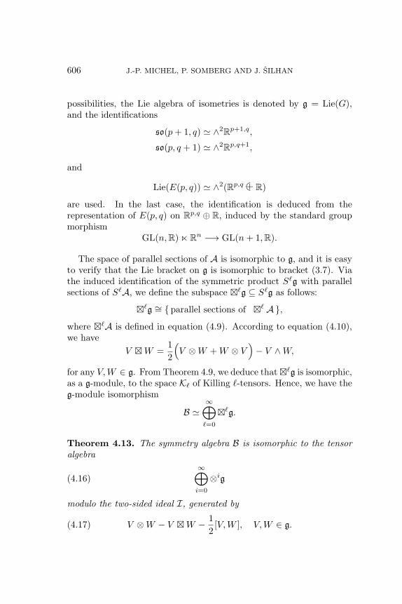
606 J.-P. MICHEL, P. SOMBERG AND J. SILHAN
possibilities, the Lie algebra of isometries is denoted by g = Lie(G),and the identifications
so(p+ 1, q) ≃ ∧2Rp+1,q,
so(p, q + 1) ≃ ∧2Rp,q+1,
and
Lie(E(p, q)) ≃ ∧2(Rp,q +�� R)
are used. In the last case, the identification is deduced from therepresentation of E(p, q) on Rp,q ⊕ R, induced by the standard groupmorphism
GL(n,R)nRn −→ GL(n+ 1,R).
The space of parallel sections of A is isomorphic to g, and it is easyto verify that the Lie bracket on g is isomorphic to bracket (3.7). Viathe induced identification of the symmetric product Sℓg with parallelsections of SℓA, we define the subspace �ℓg ⊆ Sℓg as follows:
�ℓg ∼= {parallel sections of �ℓ A},
where �ℓA is defined in equation (4.9). According to equation (4.10),we have
V �W =1
2
(V ⊗W +W ⊗ V
)− V ∧W,
for any V,W ∈ g. From Theorem 4.9, we deduce that�ℓg is isomorphic,as a g-module, to the space Kℓ of Killing ℓ-tensors. Hence, we have theg-module isomorphism
B ≃∞⊕ℓ=0
�ℓg.
Theorem 4.13. The symmetry algebra B is isomorphic to the tensoralgebra
(4.16)∞⊕i=0
⊗ig
modulo the two-sided ideal I, generated by
(4.17) V ⊗W − V �W − 1
2[V,W ], V,W ∈ g.

PROLONGATION OF SYMMETRIC KILLING TENSORS 607
Proof. First we compute the compositions DkDk, where ka, ka ∈Γ(TM) are Killing vector fields. Set K = Πka and K = Πka whereK, K ∈ g. Since ∇K = 0, definition (3.18) of DB acting on functionsyields
DkDk = KBDBKCDC
=
[1
2(KBKC +KCKB) +
1
2(KBKC −KCKB)
]DBDC
= (K � K)BCDBDC +1
2[K, K]BDB.
In the last equality, to deal with the symmetrized term, we use de-composition (4.10) and the identity D[B1B2DC1C2] = 0, which can beeasily verified. To deal with the skew-symmetrized term, we use equa-tion (3.7).
The computation of DkDk shows that all elements of the form (4.17)are in the ideal. Since there is a vector space isomorphism( ∞⊕
ℓ=0
⊗ℓg
)/I ∼=
∞⊕ℓ=0
�ℓg,
it remains to show that elements in �ℓg ∼= Kℓ indeed give rise to non-zero ℓth order symmetries. This follows from Corollary 4.12. The proofis complete. �
Passage from tensor algebra to the universal enveloping algebra U(g)means to substitute
V ⊗W =1
2
(V ⊗W +W ⊗ V
)− 1
2
(V ⊗W −W ⊗ V
)and quotient through the two-sided ideal generated by
V ⊗W −W ⊗ V = [V,W ], V,W ∈ g.
Accordingly, we obtain the following.
Corollary 4.14. The symmetry algebra B is isomorphic to the uni-versal enveloping algebra U(g) modulo the two-sided ideal generated byV ∧W for V,W ∈ g, or equivalently, by
(4.18) V ⊗W +W ⊗ V − 2V �W, V,W ∈ g.

608 J.-P. MICHEL, P. SOMBERG AND J. SILHAN
4.4. Examples of commuting symmetries. The recursion tractorformula (4.14) for commuting symmetries Dk can be transformed intoan explicit formula for Dk, expressed in terms of the Levi-Civitaconnection ∇ and the curvature J, by equations (3.18) and (4.6). Inwhat follows, we compute the explicit commuting symmetries up toorder 3 acting on E .
We use tractor form indices
A = [A1A2], B = [B1B2], C = [C1C2],
and form indices
a = [a1a2], b = [b1b2], c = [c1c2].
For a Killing vector field ka ∈ Ea, we have
(4.19) KA = (Πk)A = YAa k
a +1
2ZA
a∇[a1
ka2], DAf = 2Ya
A∇af.
Hence, the symmetry Dkf = KADAf = ka∇af coincides with the Liederivative along the Killing vector field ka.
For a Killing 2-tensor kbc ∈ E(bc), we obtain from equation (4.11),
KAB = (Π(2)k)BC = YBb YC
c kbc +
1
3
(YB
b ZCc + YC
b ZBc
)∇c1kc
2b(4.20)
+1
2ZB
bZCc
[1
3∇b1∇c1kb
2c2 +2
nJgb
1c1kb2c2
].
SinceDBDCf = 4Yb
BZ cCgbc0∇c1f + 4Yb
BYcC∇b∇cf,
by equation (3.18), we obtain
Dk = KBCDBDCf = kbc∇b∇cf + (∇rkrc)∇cf.
Note that KBChBC is a constant, and, using ∇akrr = −2∇rkar, which
follows from3gbc∇(akbc) = ∇akrr + 2∇rk
ar = 0,
a short computation reveals its value
KBChBC =1
4
[−∇r∇sσ
rs +2(n+ 1)
nJkrr
].

PROLONGATION OF SYMMETRIC KILLING TENSORS 609
Thus, the modification of Dk by any multiple of
∇r∇skrs − 2(n+ 1)
nJkrr,
is again a symmetry of ∆. This means that there is no unique formula,written in terms of kab, for a symmetry. This is in contrast with thecase of conformal symmetries [8].
Now, we consider Killing 3-tensors kabc ∈ E(abc). Then,
gcd∇(akbcd) = 3∇rkrab + 3∇akbrr = 0,
and, applying ∇a, we obtain ∇r∇skrsa+∆karr = 0. Summarizing, we
obtain
∇rkrab = −∇akbrr, ∇r∇sk
rsa = −∆karr and ∇rkrs
s = 0,
where the last equality is the trace of ∇rkrab + ∇akbrr = 0. Now,
computing Π(3)k, which requires the application of Π in equation (4.5)to equation (4.11), results in
KABC =(Π(3)k
)ABC= YA
a YBb YC
c kabc
+1
4
(YA
a YBb ZC
c + YCa YA
b ZBc + YB
a YCb ZA
c
)∇c1kc
2ab
+1
3
(YA
a ZBbZC
c + YCa ZA
bZBc + YB
a ZCbZA
c
)×[1
4∇b1∇c1kb
2c2a +2
nJgb
1c1kb2c2a
]+ ZA
aZBbZC
cψabc
for some ψabc, which we do not need to compute. Furthermore,
DADBDCf = 8YaAZb
BZ cCgab1gb2c1∇c2f
+ 16YaAYb
BZ cCgc1(a∇b)∇c2f(4.21)
+ 8YaAZb
BYcCgab1∇c∇b2f
+ 8YaAYb
BYcC
[∇a∇b∇cf −
4
nJgb[a∇c]f
],

610 J.-P. MICHEL, P. SOMBERG AND J. SILHAN
by equation (3.18). Combining the previous two displays yields
Dk = KABCDADBDCf = kabc∇a∇b∇cf(4.22)
+3
2(∇rk
rbc)∇b∇cf
+1
4(∇r∇sk
rsc)∇cf −n− 1
2nJkcrr∇cf.
By construction, the vector field (Π(2)k)aBChBC is Killing. Usingequations (3.14), (4.11) and (4.21), one easily computes
(Π(2)k)aBChBC = − 1
12
[∇r∇sk
rsa − 4(n+ 2)
nJkarr
].
Thus, symmetry Dk can be modified by a multiple of the operator[∇r∇sk
rsa − 4(n+ 2)
nJkarr
]∇af.
Remark 4.15. Let ℓ ∈ N and k ∈ Kℓ. If the curvature of metric gvanishes, i.e., M is locally isomorphic to the pseudo-Euclidean spaceRp,q, straightforward computation shows that
Dk =ℓ∑
i=0
1
2i
(ℓ
i
)(∇a1 · · · ∇aik
a1···aℓ)∇ai+1 · · ·∇aℓ
is a commuting symmetry of ∆. This can also be deduced fromproperties of the Weyl quantization of T ∗Rp,q, namely, Dk coincideswith the Weyl quantization of k, and the symplectic equivariance ofthe Weyl quantization, see, e.g., [10], yields the equalities [∆,Dk] =[g, k]S = 0. Here, [·, ·]S denotes the Schouten bracket of symmetrictensors and D[g,k]S = 0 is equivalent to the Killing equation.
Remark 4.16. Let ℓ ∈ N and k ∈ Kℓ. If k is trace-free, thenstraightforward computation shows that
Dk = ka1···aℓ∇a1 · · · ∇aℓ
is a commuting symmetry of ∆. The trace-free Killing tensors arethose which are also conformal, and this allows for comparison ofour results with the work of Eastwood [8]. Out of conformal Killingtensors V , he explicitly built conformal symmetries of the Laplacian,i.e., differential operators DV
1 and DV2 with principal symbol V such

PROLONGATION OF SYMMETRIC KILLING TENSORS 611
that DV2 ∆ = ∆DV
1 . The lower order terms involve divergences andcontractions of V with the trace-free Ricci tensor. On a space ofconstant curvature, with V = k a trace-free Killing tensor, bothdivergences and contractions vanish, see, e.g., equation (4.21), and weobtain Dk
1 = Dk2 = Dk. In [8], the symmetries built out of trace-
free Killing tensors are commuting symmetries of the Laplacian andcoincide with the symmetries constructed in our article. Note thattrace components correspond to trivial conformal symmetries in thesense of [8]. This prevents comparison of our results with those of [8]for general Killing tensors.
5. Riemannian geometry via projective geometry. Overdeter-mined equations for Killing tensors are projectively invariant [9], so itis natural to consider their prolongation within the framework of pro-jective geometry. As this is an example of parabolic geometry, we canemploy the general invariant theory for this class of structures, [5]. Weshall observe that several results obtained in the previous section thenfollow immediately.
Recall that we are interested in manifolds of constant curvature.These are conformally flat, and thus, projectively flat as well, seeequation (5.1), that is, we will consider locally flat projective structures.
5.1. Tractor calculus in projective geometry. We shall brieflyrecall invariant calculus on projective manifolds, see [1] for moredetails. A projective structure on a manifoldM is given by a class [∇] ofspecial affine connections with the same geodesics as unparametrizedcurves, where special indicates that there is a parallel volume formfor every connection in [∇]. These connections are parametrized bynowhere vanishing sections of projective density bundles E(1). We shallalso assume orientability, characterized by a compatible volume form
ϵa1···an ∈ E[a1···an](n+ 1) ∼= E ,
parallel for every affine connection in [∇]. The decomposition of thecurvature of ∇ is
(5.1) Rabcd = Cab
cd + 2δ c
[aPb]d,
where Pab is the projective Schouten tensor and Cabcd = Cab
cd, that
is, conformal and projective Weyl tensors coincide. Note that, for the

612 J.-P. MICHEL, P. SOMBERG AND J. SILHAN
Levi-Civita connection ∇ of an Einstein metric g, the curvature is alsoof the form (2.1), and the relation between projective and RiemannianSchouten tensors is Pab = 2Pab, see [11].
We define the standard tractor bundle and its dual by their spaces
of sections EA and EA, respectively, as
EA =Ea(−1)
+��E(−1)
and EA =E(1)+��Ea(1)
;
see [1] for the meaning of the semi-direct product +��
. The choice ofa connection in the class [∇] turns the previous display into the directsum decomposition. These bundles are equipped with the projectivelyinvariant tractor connection which we denote by ∇. Choosing ∇ in theprojective class, ∇ is explicitly given by the formulas
∇a
(νb
ρ
)=
(∇aν
b + δ baρ
∇aρ− Pabνb
)and ∇a
(σµb
)=
(∇aσ − µa
∇aµb + Pabσ
);
(5.2)
see [1] for details. Here, νa ∈ Ea(−1), ρ ∈ E(−1), σ ∈ E(1) and
µa ∈ Ea(1). We extend the connection ∇ to the tensor products of EA
by the Leibniz rule. Also note that the structure of the tractor bundle
E [AB]and of its dual is given by
(5.3) E [AB]=E [ab](−2)
+��
Ea(−2)and E [AB] =
Ea(2)+��
E[ab](2).
In what follows, we shall use the tractor bundle
E B
A = EA ⊗ EB=
Ea+��
E ba ⊕ E+��Ea
,(5.4)
where the trace-free part of E B
A is isomorphic to the projective adjointtractor bundle. Analogously to equation (3.15), we define the projec-
PROLONGATION OF SYMMETRIC KILLING TENSORS 613
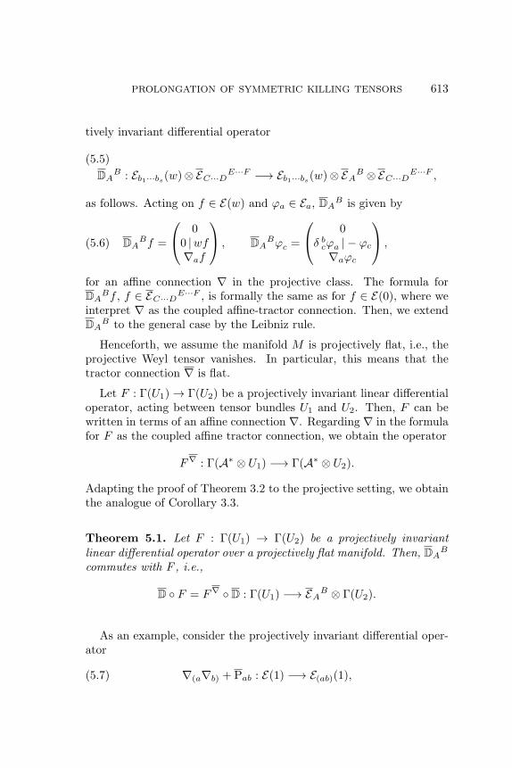
tively invariant differential operator
(5.5)
DAB : Eb1···bs(w)⊗EC···D
E···F −→ Eb1···bs(w)⊗EAB ⊗EC···DE···F ,
as follows. Acting on f ∈ E(w) and φa ∈ Ea, DAB is given by
DABf =
00 |wf∇af
, DABφc =
0δ bcφa | − φc
∇aφc
,(5.6)
for an affine connection ∇ in the projective class. The formula forDA
Bf , f ∈ EC···DE···F , is formally the same as for f ∈ E(0), where we
interpret ∇ as the coupled affine-tractor connection. Then, we extendDA
B to the general case by the Leibniz rule.
Henceforth, we assume the manifold M is projectively flat, i.e., theprojective Weyl tensor vanishes. In particular, this means that thetractor connection ∇ is flat.
Let F : Γ(U1)→ Γ(U2) be a projectively invariant linear differentialoperator, acting between tensor bundles U1 and U2. Then, F can bewritten in terms of an affine connection ∇. Regarding ∇ in the formulafor F as the coupled affine tractor connection, we obtain the operator
F∇ : Γ(A∗ ⊗ U1) −→ Γ(A∗ ⊗ U2).
Adapting the proof of Theorem 3.2 to the projective setting, we obtainthe analogue of Corollary 3.3.
Theorem 5.1. Let F : Γ(U1) → Γ(U2) be a projectively invariantlinear differential operator over a projectively flat manifold. Then, DA
B
commutes with F , i.e.,
D ◦ F = F∇ ◦ D : Γ(U1) −→ EAB ⊗ Γ(U2).
As an example, consider the projectively invariant differential oper-ator
(5.7) ∇(a∇b) + Pab : E(1) −→ E(ab)(1),

614 J.-P. MICHEL, P. SOMBERG AND J. SILHAN
see e.g., [4]. Projective invariance and Theorem 5.1 imply
D B1
A1· · ·D Bℓ
Aℓ
(∇(a∇b) + Pab
)(5.8)
=(∇(a∇b) + Pab
)D B1
A1· · ·D Bℓ
Aℓ,
where ∇ on the right side denotes the coupled affine tractor connection.
5.2. Killing tensors in projective geometry. Let ℓ ∈ N. We shallfocus on the PDE
∇(a0ka1···aℓ) = 0, ka1···aℓ
∈ E(a1···aℓ)(2ℓ),(5.9)
which is projectively invariant [9].
Setting EA = , we have E [AB] = , and we set
�ℓE [AB] :=
ℓ︷ ︸︸ ︷· · ·· · · SℓE [AB].
There exists a linear map
Π(ℓ)
: Ea1···aℓ(2ℓ) −→ �ℓ E [AB],
characterized by curved Casimir operators, see [6], which takes theform
(5.10) Π(ℓ)
: ka1···aℓ7−→ K [A1B1]···[AℓBℓ] =
ka1···aℓ
+��...
∈Ea1···aℓ
(2ℓ)+��...
and such that ka1···aℓis a solution of equation (5.9) if and only if
K [A1B1]···[AℓBℓ] is ∇-parallel. Note that the unspecified terms (indi-
cated by vertical dots) of K [A1B1]···[AℓBℓ] are differential in ka1···aℓ, i.e.,
the map Π(ℓ)
is given by a differential operator. In fact, this is anexample of a splitting operator, see e.g., [6] for details. It yields ananalog of Theorem 4.9.
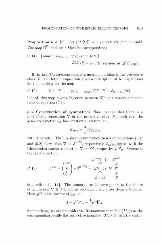
PROLONGATION OF SYMMETRIC KILLING TENSORS 615
Proposition 5.2. [2]. Let (M, [∇]) be a projectively flat manifold.
The map Π(ℓ)
induces a bijective correspondence
(5.11) {solutions ka1···aℓof equation (5.9)}1−1←→ {∇− parallel sections of �ℓ E [AB]}.
If the Levi-Civita connection of a metric g pertains to the projectiveclass [∇], the latter proposition gives a description of Killing tensorsfor the metric g via the map
(5.12) V (a1···aℓ) 7−→ ga1b1 · · · ga1b1V(a1···aℓ) ∈ E(b1···bℓ)(2ℓ).
Indeed, this map gives a bijection between Killing ℓ-tensors and solu-tions of equation (5.9).
5.3. Construction of symmetries. Now, assume that there is aLevi-Civita connection ∇ in the projective class [∇], such that theassociated metric gab has constant curvature, i.e.,
Rabcd =4
nJgc[agb]d
with J parallel. Then, a short computation based on equations (3.4)
and (5.2) shows that ∇ on E [AB], respectively, E [AB], agrees with the
Riemannian tractor connection ∇ on EA, respectively, EA. Moreover,the tractor section
(5.13) hAB =
gab02nJ
∈ E(AB)=
E(ab)(−2)+��
Ea(−2)+��E(−2)
∼=
E(ab)⊕Ea⊕E
is parallel, cf., [11]. The isomorphism ∼= corresponds to the choiceof connection ∇ ∈ [∇], and in particular, trivializes density bundles.Here, gab is the inverse of gab and
J = gabPab =1
2gabPab.
Summarizing, we shall consider the Riemannian manifold (M, g) as thecorresponding locally flat projective manifold (M, [∇]) with the distin-
616 J.-P. MICHEL, P. SOMBERG AND J. SILHAN
guished parallel section hAB . This is an example of holonomy reductionof Cartan connections [3] for the projective Cartan connection associ-ated to (M, [∇]).
For J = 0, note that hAB is non-degenerate, hence, a tractor metric.A direct computation gives the next display and Lemma 5.3:
(5.14) hP [ADPB]gab = hP [ADP
B]gab = 0.
Lemma 5.3. The explicit formula for the differential operator
hP [ADPB] : E(w) −→ E [AB](w),
written in terms of the Levi-Civita connection ∇, does not depend onw ∈ R.
We are now ready to construct the commuting symmetries of theLaplace operator. The metric g allows for identification of a tensorV a1···aℓ ∈ E(a1···aℓ) with an element in E(a1···aℓ)(2ℓ), see equation (5.12),
and we denote by V ∈ �ℓ E [AB] the corresponding tractor, obtained via
the map Π ℓ, see equation (5.10). We consider the operators
DV:= hA1C1 · · ·hAℓCℓV A1B1···AℓBℓ
DC1
B1 · · ·DCℓ
Bℓ ,(5.15)
acting on any tensor-tractor bundle U .
Lemma 5.4. The principal symbol of the differential operator D Vis
the symmetric ℓ-tensor V .
Proof. The proof is analogous to the proof of Theorem 4.11. Writingtractor sections in vertical notation, see equation (5.3), we can referto their “top” or “bottom” parts. The “top” part of V A1B1···AℓBℓ
isga1b1 · · · ga1b1V
(a1···aℓ), cf., equations (5.10) and (5.12). On the otherhand, elementary computation using equations (5.6) and (5.13) showsthat the bottom part (and the leading term) of hC[ADC
B]f is equal togab∇bf for any section f of a tensor bundle. Therefore, the bottompart of the composition
hC1[A1DC1
B1] · · ·hCℓ[AℓDCℓ
Bℓ]f
is equal to
PROLONGATION OF SYMMETRIC KILLING TENSORS 617
ga1b1∇b1 · · · gaℓbℓ∇bℓf.
This completes the proof of Lemma 5.4. �
Theorem 5.5. Let (M, g) be a pseudo-Riemannian manifold of con-stant curvature, with Levi-Civita connection ∇, and let (M, [∇]) be thecorresponding locally flat projective manifold. Then, if k is a Killingℓ-tensor, the operator
Dk: E −→ E ,
defined by equation (5.15), is a commuting symmetry of the Laplaceoperator ∆ = gab∇a∇b.
Proof. Let K ∈ �ℓE [AB] be the parallel tractor associated to k viathe composition of maps (5.11) and (5.12). Since the tractor metric his also parallel with respect to the projective tractor connection ∇, itfollows from equations (5.8) and (5.14) that
Dk(gab(∇(a∇b) + Pab)
)=
(gab(∇(a∇b) + Pab)
)Dk
: E(+1) −→ E(−1),
where we consider gab ∈ E(ab)(−2). The operator
Dk: E(w) −→ E(w),
expressed in terms of ∇, does not depend on w ∈ R by Lemma 5.3.Observing that gabPab is parallel for ∇, the theorem follows. �
Remark 5.6. Projectively invariant overdetermined operators, as theoperator defined in equation (5.7), are discussed in [9]. They allowfor analogous construction of symmetries for other Riemannian lineardifferential operators
F : Γ(U) −→ Γ(U).
Acknowledgments. The authors are grateful to A. Cap, M.G.Eastwood and A.R. Gover for their suggestion on the interpretationof our results in the framework of projective parabolic geometry.

618 J.-P. MICHEL, P. SOMBERG AND J. SILHAN
REFERENCES
1. T.N. Bailey, M.G. Eastwood and A.R. Gover, Thomas’s structure bundle forconformal, projective and related structures, Rocky Mountain J. Math. 24 (1994),1191–1217.
2. T. Branson, A. Cap, M.G. Eastwood and A.R. Gover, Prolongations ofgeometric overdetermined systems, Int. J. Math. 17 (2006), 641–664.
3. A. Cap, A.R. Gover and M. Hammerl, Projective BGG equations, algebraicsets, and compactifications of Einstein geometries, J. Lond. Math. Soc. 86 (2012),433–454.
4. , Holonomy reductions of Cartan geometries and curved orbit decom-positions, preprint, ESI 2308.
5. A. Cap and J. Slovak, Parabolic geometries I: Background and general theory,
Math. Surv. Mono. 154, American Mathematical Society, Providence, RI, 2009.
6. A. Cap and V. Soucek, Curved Casimir operators and the BGG machinery,SIGMA Sym. Int. Geom. Meth. Appl. 3 (2007), 17 pages.
7. B. Carter, Killing tensor quantum numbers and conserved currents in curvedspace, Phys. Rev. 16 (1977), 3395–3414.
8. M.G. Eastwood, Higher symmetries of the Laplacian, Ann. Math. 161 (2005),1645–1665.
9. M.G. Eastwood and A.R. Gover, The BGG complex on projective space,
SIGMA Sym. Int. Geom. Meth. Appl. 7 (2011), 18 pages.
10. G.B. Folland, Harmonic analysis in phase space, Ann. Math. Stud. 122,
Princeton University Press, Princeton, 1989.
11. A.R. Gover and H. Macbeth, Detecting Einstein geodesics: Einstein metricsin projective and conformal geometry, arXiv: http://arxiv.org/abs/1212.6286.
12. A.R. Gover and J. Silhan, Higher symmetries of the conformal powers ofthe Laplacian on conformally flat manifolds, J. Math. Phys. 53 (2012), 26 pages.
13. B. Kostant, Verma modules and the existence of quasi-invariant differentialoperators, in Non-commutative harmonic analysis, Lect. Notes Math. 466, SpringerVerlag, New York, 1975.
14. , Holonomy and the Lie algebra of infinitesimal motions of a Rie-mannian manifold, Trans. Amer. Math. Soc. 80 (1955), 528–542.
15. R.G. McLenaghan, R. Milsan and R.G. Smirnov, Killing tensors as irre-
ducible representations of the general linear group, C.R. Math. Acad. Sci. Paris339 (2004), 621–624.
16. J.-Ph. Michel, Higher symmetries of Laplacian via quantization, Ann. Inst.
Fourier 64 (2014), 1581–1609.
17. M. Takeuchi, Killing tensor fields on spaces of constant curvature, Tsukuba
J. Math. 7 (1983), 233–255.

PROLONGATION OF SYMMETRIC KILLING TENSORS 619
18. J.A. Wolf, Spaces of constant curvature, McGraw-Hill, New York, 1967.
University of Liege, Grande Traverse, 12, Sart-Tilman, B-4000 Liege,BelgiumEmail address: [email protected]
Mathematical Institute, Charles University, Sokolovska 83, 186 75, Prague8, Czech Republic
Email address: [email protected]
Institute of Mathematics and Statistics, Masaryk University, Building 08,
Kotlarska 2, Brno, 611 37 Czech RepublicEmail address: [email protected]