robert stengel, aircraft flight dynamics mae 331, 2016stengel/mae331lecture11.pdf · numerical...
TRANSCRIPT

Linearized Equations of Motion!Robert Stengel, Aircraft Flight Dynamics!
MAE 331, 2016
Copyright 2016 by Robert Stengel. All rights reserved. For educational use only.http://www.princeton.edu/~stengel/MAE331.html
http://www.princeton.edu/~stengel/FlightDynamics.html
Reading:!Flight Dynamics!
234-242, 255-266, 274-297, 321-325, 329-330!
Develop linear equations to describe small perturbational motions
Apply to aircraft dynamic equations
Learning Objectives
1
Assignment #6"due: End of day, Nov. 22, 2016!
•! Code the aerodynamic, thrust, and inertial properties of the HondaJet in AeroModel.m (MATLAB function for FLIGHTver2.m)
2

Review Questions!!! Describe the functions of airplane control systems:!
!! Elevator/Stabilator!!! Ailerons/Elevons!!! Rudder!!! Spoilers!
!! How can you control the yaw dynamics of a flying wing airplane?!
!! What are compensating ailerons?!!! Why aren’t all control surfaces “all moving”?!!! How are the mechanical dynamics of control systems
modeled?!!! What is a horn balance, and how does it work?!!! What are control tabs, and how do they work?!
3
•! Linear and nonlinear, time-varying and time-invariant dynamic models–! Numerical integration ( time domain )
•! Linear, time-invariant (LTI) dynamic models–! Numerical integration ( time domain )–! State transition ( time domain )–! Transfer functions ( frequency domain )
How Is System Response Calculated?
4

Integration Algorithms
•! Rectangular (Euler) Integration
x(tk ) = x(tk!1)+"x(tk!1,tk )# x(tk!1)+ f x(tk!1),u(tk!1),w(tk!1)[ ]" t
" t = tk ! tk!1
•! Trapezoidal (modified Euler) Integration (~MATLAB s ode23)
x(tk ) ! x(tk"1)+12#x1 +#x2[ ]
where#x1 = f x(tk"1),u(tk"1),w(tk"1)[ ]# t
#x2 = f x(tk"1)+#x1,u(tk ),w(tk )[ ]# tSee MATLAB manual for descriptions of ode45 and ode15s
5
•! Exact x T( ) = x 0( ) + f x t( ),u t( ),w t( )!" #$0
T
% dt
Numerical Integration:MATLAB Ordinary Differential Equation
Solvers*
•! Explicit Runge-Kutta Algorithm
•! Numerical Differentiation Formula
* http://www.mathworks.com/access/helpdesk/help/techdoc/index.html?/access/helpdesk/help/techdoc/ref/ode23.html. Shampine, L. F. and M. W. Reichelt, "The MATLAB ODE Suite," SIAM Journal on Scientific Computing, Vol. 18, 1997, pp 1-22.
•! Adams-Bashforth-Moulton Algorithm
•! Modified Rosenbrock Method
•! Trapezoidal Rule
•! Trapezoidal Rule w/Back Differentiation
6

Nominal and Actual Trajectories•! Nominal (or reference) trajectory and
control history
xN (t), uN (t),wN (t){ } for t in [to,t f ]
•! Actual trajectory perturbed by–! Small initial condition variation, !!xo(to)–! Small control variation, !!u(t)
x(t), u(t),w(t){ } for t in [to,t f ]
= xN (t)+ !x(t), uN (t)+ !u(t),wN (t)+ !w(t){ }
x : dynamic stateu : control inputw : disturbance input
7
Both Paths Satisfy the Dynamic Equations
Dynamic models for the actual and the nominal problems are the same
!xN (t) = f[xN (t),uN (t),wN (t)], xN to( ) given
!x(t) = f[x(t),u(t),w(t)], x to( ) given
!x(t) = !xN (t)+ !!x(t)x(t) = xN (t)+ !x(t)
"#$
%$
&'$
($ in to,t f)* +,
!x(to ) = x(to ) " xN (to )
!u(t) = u(t) " uN (t)!w(t) = w(t) " wN (t)
#$%
&%
'(%
)% in to,t f*+ ,-
Differences in initial condition and forcing ...
... perturb rate of change and the state
8

Approximate Neighboring Trajectory as a Linear Perturbation
to the Nominal Trajectory
!x(t) = !xN (t)+ !!x(t)
" f[xN (t),uN (t),wN (t),t]+# f#x
!x(t)+ # f#u
!u(t)+ # f#w
!w(t)
Approximate the new trajectory as the sum of the nominal path plus a linear perturbation
!xN (t) = f[xN (t),uN (t),wN (t),t]!x(t) = !xN (t)+ !!x(t) = f[xN (t)+ !x(t),uN (t)+ !u(t),wN (t)+ !w(t),t]
9
Linearized Equation Approximates Perturbation Dynamics
•! Solve for the nominal and perturbation trajectories separately
!xN (t) = f[xN (t),uN (t),wN (t),t], xN to( ) given
!!x(t) " # f#x x=xN (t )
u=uN (t )w=wN (t )
!x(t)$
%
&&&
'
(
)))+# f#u x=xN (t )
u=uN (t )w=wN (t )
!u(t)$
%
&&&
'
(
)))+# f#w x=xN (t )
u=uN (t )w=wN (t )
!w(t)$
%
&&&
'
(
)))
" F(t)!x(t)+G(t)!u(t)+L(t)!w(t), !x to( ) given
dim(x) = n !1dim(u) = m !1dim(w) = s !1
dim(!x) = n "1dim(!u) = m "1dim(!w) = s "1
Nominal Equation
Perturbation Equation
10

Jacobian Matrices Express Solution Sensitivity to Small Perturbations
Stability matrix, F, is square
F(t) = ! f!x x=xN (t )
u=uN (t )w=wN (t )
=
! f1! x1
!! f1! xn
! ! !! fn! x1
!! fn! xn
"
#
$$$$$$
%
&
''''''x=xN (t )u=uN (t )w=wN (t )
dim(F) = n ! n
11
Sensitivity to Control Perturbations, G
G(t) = ! f!u x=xN (t )
u=uN (t )w=wN (t )
=
! f1!u1
!! f1!um
! ! !! fn!u1
!! fn!um
"
#
$$$$$$
%
&
''''''x=xN (t )u=uN (t )w=wN (t )dim(G) = n ! m
12
L(t) = ! f!w x=xN (t )
u=uN (t )w=wN (t )
=
! f1!w1
!! f1!ws
! ! !! fn!w1
!! fn!ws
"
#
$$$$$$
%
&
''''''x=xN (t )u=uN (t )w=wN (t )
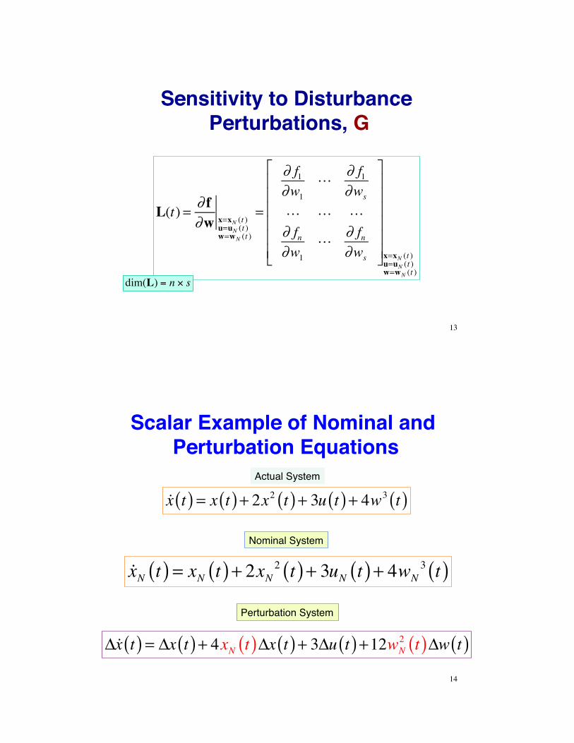
dim(L) = n ! s
13
Sensitivity to Disturbance Perturbations, G
Scalar Example of Nominal and Perturbation Equations
!x t( ) = x t( ) + 2x2 t( ) + 3u t( ) + 4w3 t( )
!!x t( ) = !x t( ) + 4xN t( )!x t( ) + 3!u t( ) +12wN2 t( )!w t( )
14
Actual System
Nominal System
Perturbation System
!xN t( ) = xN t( ) + 2xN 2 t( ) + 3uN t( ) + 4wN3 t( )

Comparison of Damped Linear and Nonlinear Systems
!x1(t) = x2 (t)!x2 (t) = !10x1(t)!10x1
3(t)! x2 (t)
Linear plus Stiffening Cubic Spring
Linear plus Weakening Cubic Spring
!x1(t) = x2 (t)!x2 (t) = !10x1(t)+ 0.8x1
3(t)! x2 (t)
!x1(t) = x2 (t)!x2 (t) = !10x1(t)! x2 (t)
Linear Spring Linear Spring Force vs. Displacement
Spring Damper
Displacement
Rate of Change
15
Cubic Spring Force vs. Displacement
Cubic Spring Force vs. Displacement
MATLAB Simulation of Linear and Nonlinear Dynamic Systems
MATLAB Main Script
% Nonlinear and Linear Examples clear tspan = [0 10]; xo = [0, 10]; [t1,x1 = ode23('NonLin',tspan,xo); xo = [0, 1]; [t2,x2] = ode23('NonLin',tspan,xo); xo = [0, 10]; [t3,x3] = ode23('Lin',tspan,xo); xo = [0, 1]; [t4,x4] = ode23('Lin',tspan,xo); subplot(2,1,1) plot(t1,x1(:,1),'k',t2,x2(:,1),'b',t3,x3(:,1),'r',t4,x4(:,1),'g') ylabel('Position'), grid subplot(2,1,2) plot(t1,x1(:,2),'k',t2,x2(:,2),'b',t3,x3(:,2),'r',t4,x4(:,2),'g') xlabel('Time'), ylabel('Rate'), grid
Linear System
function xdot = Lin(t,x)% Linear Ordinary Differential Equation% x(1) = Position% x(2) = Ratexdot = [x(2) -10*x(1) - x(2)];
Nonlinear System
function xdot = NonLin(t,x)% Nonlinear Ordinary Differential Equation% x(1) = Position% x(2) = Ratexdot = [x(2) -10*x(1) + 0.8*x(1)^3 - x(2)];
˙ x 1(t) = x2(t)˙ x 2(t) = "10x1(t) " x2(t)
˙ x 1(t) = x2(t)˙ x 2(t) = "10x1(t) + 0.8x1
3(t) " x2(t)
16

Linear and Stiffening Cubic Springs: Small and
Large Initial Conditions
Linear and nonlinear responses are indistinguishable with small initial condition17
Cubic term
Linear and Weakening Cubic Springs: Small and Large Initial Conditions
18
Cubic term

Linear, Time-Varying (LTV) Approximation of
Perturbation Dynamics!
19
Stiffening Linear-Cubic Spring Example
Nonlinear, time-invariant (NTI) equation
!x1(t) = f1 = x2 (t)!x2 (t) = f2 = !10x1(t)!10x1
3(t)! x2 (t)Integrate equations to produce nominal path
x1N (0)
x2N (0)
!
"
##
$
%
&&'
f1Nf2N
!
"
##
$
%
&&dt'
0
t f
(x1N (t)
x2N (t)
!
"
##
$
%
&&
in 0,t f!" $%
Analytical evaluation of partial derivatives! f1! x1
= 0; ! f1! x2
= 1
! f2! x1
= "10 " 30x1N2 (t); ! f2
! x2= "1
! f1!u
= 0; ! f1!w
= 0
! f2!u
= 0; ! f2!w
= 020

Nominal (NTI) and Perturbation (LTV) Dynamic Equations
!xN (t) = f[xN (t)], xN (0) given! ! ! ! ! ! ! ! ! ! ! ! ! ! ! !
!x1N (t) = x2N (t)
!x2N (t) = !10x1N (t)!10x1N3(t)! x2N (t)
!!x(t) = F(t)!x(t), !x(0) given" " " " " " " " " " " " " " " "
!!x1(t)!!x2 (t)
#
$%%
&
'((=
0 1" 10 + 30x1N
2 (t)( ) "1
#
$%%
&
'((
!x1(t)!x2 (t)
#
$%%
&
'((
x1N (0)
x2N (0)
!
"
##
$
%
&&= 0
9
!
"#
$
%&
Nonlinear, time-invariant (NTI) nominal equation
Perturbations approximated by linear, time-varying (LTV) equation
!x1(0)!x2 (0)
"
#$$
%
&''= 0
1
"
#$
%
&'
Example
Example
21
Comparison of Approximate and Exact Solutions
xN (t)!x(t)xN (t)+!x(t)x(t)
Initial Conditionsx2N (0)= 9!x2 (0)=1x2N (t)+!x2 (t)=10x2 (t)=10
!xN (t)!!x(t)!xN (t) + !!x(t)!x(t) 22

Suppose Nominal Initial Condition is Zero
!xN (t) = f[xN (t)], xN (0) = 0, xN (t) = 0 in 0,![ ]
Nominal solution remains at equilibrium
Perturbation equation is linear and time-invariant (LTI)
!!x1(t)!!x2 (t)
"
#$$
%
&''=
0 1(10( 30 0( )"# %& (1
"
#
$$
%
&
''
!x1(t)!x2 (t)
"
#$$
%
&''
23
Separation of the !Equations of Motion into Longitudinal and Lateral-
Directional Sets!
24
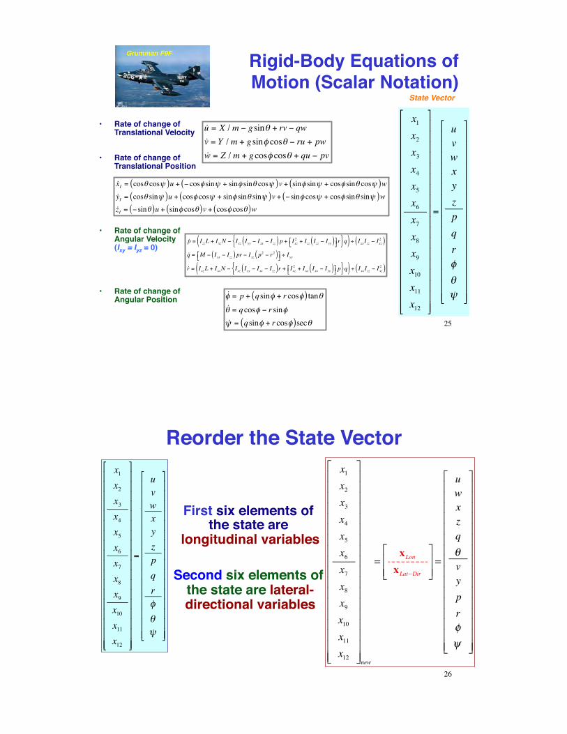
Rigid-Body Equations of Motion (Scalar Notation)
•! Rate of change of Translational Position
•! Rate of change of Angular Position
•! Rate of change of Translational Velocity
•! Rate of change of Angular Velocity (Ixy = Iyz = 0)
x1x2x3x4x5x6x7x8x9x10x11x12
!
"
##################
$
%
&&&&&&&&&&&&&&&&&&
=
uvwxyzpqr'
()
!
"
################
$
%
&&&&&&&&&&&&&&&&
State Vector
!u = X / m ! gsin" + rv ! qw!v = Y / m + gsin# cos" ! ru + pw!w = Z / m + gcos# cos" + qu ! pv
!xI = cos! cos"( )u + # cos$ sin" + sin$ sin! cos"( )v + sin$ sin" + cos$ sin! cos"( )w!yI = cos! sin"( )u + cos$ cos" + sin$ sin! sin"( )v + # sin$ cos" + cos$ sin! sin"( )w!zI = # sin!( )u + sin$ cos!( )v + cos$ cos!( )w
!! = p + qsin! + r cos!( ) tan"!" = qcos! # r sin!!$ = qsin! + r cos!( )sec"
Grumman F9F
!p = IzzL + IxzN ! Ixz Iyy ! Ixx ! Izz( ) p + Ixz2 + Izz Izz ! Iyy( )"# $%r{ }q( ) ÷ Ixx Izz ! Ixz
2( )!q = M ! Ixx ! Izz( ) pr ! Ixz p2 ! r2( )"# $% ÷ Iyy
!r = IxzL + IxxN ! Ixz Iyy ! Ixx ! Izz( )r + Ixz2 + Ixx Ixx ! Iyy( )"# $% p{ }q( ) ÷ Ixx Izz ! Ixz
2( )
25
Reorder the State Vector
x1x2x3x4x5x6x7x8x9x10x11x12
!
"
##################
$
%
&&&&&&&&&&&&&&&&&&new
=xLonxLat'Dir
!
"##
$
%&&=
uwxzq(vypr)*
!
"
################
$
%
&&&&&&&&&&&&&&&&
First six elements of the state are
longitudinal variables
Second six elements of the state are lateral-directional variables
x1x2x3x4x5x6x7x8x9x10x11x12
!
"
##################
$
%
&&&&&&&&&&&&&&&&&&
=
uvwxyzpqr'
()
!
"
################
$
%
&&&&&&&&&&&&&&&&
26

Longitudinal Equations of Motion Dynamics of velocity, position, angular rate,
and angle primarily in the vertical plane
!u = X /m ! gsin" + rv ! qw " !x1 = f1!w = Z /m + gcos# cos" + qu ! pv " !x2 = f2
!xLon (t) = f[xLon (t),uLon (t),wLon (t)]
!xI = cos! cos"( )u +#cos$ sin" + sin$ sin! cos"( )v + sin$ sin" + cos$ sin! cos"( )w " !x3 = f3!zI = #sin!( )u + sin$ cos!( )v + cos$ cos!( )w " !x4 = f4
!q = M ! Ixx ! Izz( ) pr ! Ixz p2 ! r2( )"# $% ÷ Iyy " !x5 = f5!& = qcos' ! r sin' " !x6 = f6
27
!v = Y /m + gsin! cos" # ru + pw " !x7 = f7!yI = cos" sin$( )u + cos! cos$ + sin! sin" sin$( )v +
#sin! cos$ + cos! sin" sin$( )w " !x8 = f8
Lateral-Directional Equations of Motion
!xLD (t) = f[xLD (t),uLD (t),wLD (t)]
!p = IzzL + IxzN ! Ixz Iyy ! Ixx ! Izz( ) p + Ixz2 + Izz Izz ! Iyy( )"# $%r{ }q( ) ÷ Ixx Izz ! Ixz
2( ) " !x9 = f9
!r = IxzL + IxxN ! Ixz Iyy ! Ixx ! Izz( )r + Ixz2 + Ixx Ixx ! Iyy( )"# $% p{ }q( ) ÷ Ixx Izz ! Ixz
2( ) " !x10 = f10
!! = p + qsin! + r cos!( ) tan" " !x11 = f11!# = qsin! + r cos!( )sec" " !x12 = f12
Dynamics of velocity, position, angular rate, and angle primarily out of the vertical plane
28
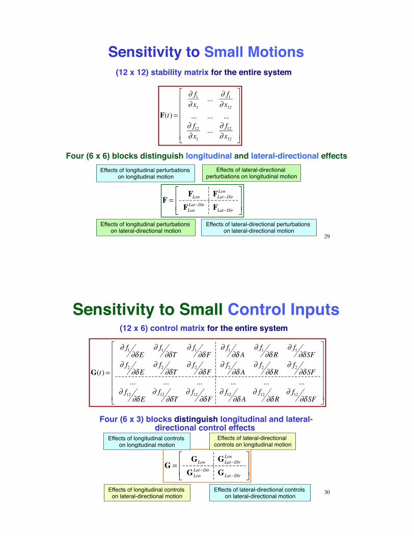
Sensitivity to Small Motions(12 x 12) stability matrix for the entire system
F(t) =
! f1! x1
... ! f1! x12
... ... ...! f12! x1
... ! f12! x12
"
#
$$$$$$
%
&
''''''
Four (6 x 6) blocks distinguish longitudinal and lateral-directional effects
F =FLon FLat!Dir
Lon
FLonLat!Dir FLat!Dir
"
#$$
%
&''
Effects of longitudinal perturbations on longitudinal motion
Effects of longitudinal perturbations on lateral-directional motion
Effects of lateral-directional perturbations on longitudinal motion
Effects of lateral-directional perturbations on lateral-directional motion
29
Sensitivity to Small Control Inputs
Four (6 x 3) blocks distinguish longitudinal and lateral-directional control effects
G =GLon GLat!Dir
Lon
GLonLat!Dir GLat!Dir
"
#$$
%
&''
Effects of longitudinal controls on longitudinal motion
Effects of longitudinal controls on lateral-directional motion
Effects of lateral-directional controls on longitudinal motion
Effects of lateral-directional controls on lateral-directional motion 30
(12 x 6) control matrix for the entire system
G(t) =
! f1!"E
! f1!"T
! f1!"F
! f1!"A
! f1!"R
! f1!"SF
! f2!"E
! f2!"T
! f2!"F
! f2!"A
! f2!"R
! f2!"SF
... ... ... ... ... ...! f12
!"E! f12
!"T! f12
!"F! f12
!"A! f12
!"R! f12
!"SF
#
$
%%%%%%%
&
'
(((((((

Sensitivity to Small Disturbance InputsDisturbance input vector and perturbation
Four (6 x 3) blocks distinguish longitudinal and lateral-directional effects
L =LLon LLat!Dir
Lon
LLonLat!Dir LLat!Dir
"
#$$
%
&''
Effects of longitudinal disturbances on longitudinal motion
Effects of longitudinal disturbances on lateral-directional motion
Effects of lateral-directional disturbances on longitudinal motion
Effects of lateral-directional disturbances on lateral-directional motion
w(t) =
uw (t)ww (t)qw (t)vw (t)pw (t)rw (t)
!
"
########
$
%
&&&&&&&&
Axial wind, m / sNormal wind, m / s
Pitching wind shear, deg / s or rad / sLateral wind, m / s
Rolling wind shear, deg / s or rad / sYawing wind shear, deg / s or rad / s
!w(t) =
!uw (t)!ww (t)!qw (t)!vw (t)!pw (t)!rw (t)
"
#
$$$$$$$$
%
&
''''''''
31
Decoupling Approximation for Small Perturbations from Steady, Level Flight!
32

Restrict the Nominal Flight Path to the Vertical Plane
Nominal longitudinal equations reduce to
Nominal lateral-directional motions are zerox1x2x3x4x5x6x7x8x9x10x11x12
!
"
##################
$
%
&&&&&&&&&&&&&&&&&&N
=xLonxLat'Dir
!
"##
$
%&&N
=
uNwN
xNzNqN(N
000000
!
"
################
$
%
&&&&&&&&&&&&&&&&
!uN = X /m ! gsin"N ! qNwN
!wN = Z /m + gcos"N + qNuN!xIN = cos"N( )uN + sin"N( )wN
!zIN = !sin"N( )uN + cos"N( )wN
!qN = MIyy
!"N = qN
!xLat!DirN = 0xLat!DirN = 0
Nominal State Vector
33
Restrict the Nominal Flight Path to Steady, Level Flight
•! Calculate conditions for trimmed (equilibrium) flight–! See Flight Dynamics and FLIGHT program for a
solution method
0 = X /m ! gsin"N ! qNwN
0 = Z /m + gcos"N + qNuNVN = cos"N( )uN + sin"N( )wN
0 = !sin"N( )uN + cos"N( )wN
0 = MIyy
0 = qN
Trimmed State Vector is constant
•! Specify nominal airspeed (VN) and altitude (hN = –zN)
uwxzq!
"
#
$$$$$$$
%
&
'''''''Trim
=
uTrimwTrim
VN t ( t0( )zN0
!Trim
"
#
$$$$$$$$
%
&
''''''''
34

Small Longitudinal and Lateral-Directional Perturbation Effects•! Assume the airplane is symmetric and its
nominal path is steady, level flight–! Small longitudinal and lateral-directional
perturbations are approximately uncoupled from each other
–! (12 x 12) system is •! block diagonal•! constant, i.e., linear, time-invariant (LTI)•! decoupled into two separate (6 x 6) systems
F =FLon 00 FLat!Dir
"
#$$
%
&''
G =GLon 00 GLat!Dir
"
#$$
%
&''
L =LLon 00 LLat!Dir
"
#$$
%
&''
35
!!xLon (t) = FLon!xLon (t) +GLon!uLon (t) + LLon!wLon (t)
!xLon =
!x1!x2!x3!x4!x5!x6
"
#
$$$$$$$$
%
&
''''''''Lon
=
!u!w!x!z!q!(
"
#
$$$$$$$
%
&
'''''''
(6 x 6) LTI Longitudinal Perturbation Model
!uLon =!"T!"E!"F
#
$
%%%
&
'
(((
!wLon =
!uwind!wwind
!qwind
"
#
$$$
%
&
'''
Dynamic Equation
State VectorControl Vector
DisturbanceVector
36

LTI Longitudinal Response to Initial Pitch Rate
37
(6 x 6) LTI Lateral-Directional Perturbation Model
!!xLat"Dir (t) = FLat"Dir!xLat"Dir (t) +GLat"Dir!uLat"Dir (t) + LLat"Dir!wLat"Dir (t)
!xLat"Dir =
!x1!x2!x3!x4!x5!x6
#
$
%%%%%%%%
&
'
((((((((Lat"Dir
=
!v!y!p!r!)
!*
#
$
%%%%%%%%
&
'
((((((((
!uLat"Dir =!#A!#R!#SF
$
%
&&&
'
(
)))
!wLon =
!vwind!pwind!rwind
"
#
$$$
%
&
'''
Dynamic Equation
State VectorControl Vector
DisturbanceVector
38

LTI Lateral-Directional Response to Initial Yaw Rate
39
Next Time:!Longitudinal Dynamics!
Reading:!Flight Dynamics!
452-464, 482-486!Airplane Stability and Control!
Chapter 7!
40
•! 6th-order -> 4th-order -> hybrid equations•! Dynamic stability derivatives •! Long-period (phugoid) mode•! Short-period mode
Learning Objectives

SSuupppplleemmeennttaall MMaatteerriiaall
41
How Do We Calculate the Partial Derivatives?
•! Numerically–!First differences in f(x,u,w)
•! Analytically–!Symbolic evaluation of analytical
models of F, G, and L
F(t) = !f!x x=xN (t )
u=uN (t )w=wN (t )
G(t) = !f!u x=xN (t )
u=uN (t )w=wN (t )
L(t) = !f!w x=xN (t )
u=uN (t )w=wN (t )
42

Numerical Estimation of the Jacobian Matrix, F(t)
! f1!x1
t( ) "
f1
x1 + #x1( )x2!xn
$
%
&&&&&
'
(
)))))
* f1
x1 * #x1( )x2!xn
$
%
&&&&&
'
(
))))) x=xN (t )u=uN (t )w=wN (t )
2#x1; ! f1
!x2t( ) "
f1
x1x2 + #x2( )!xn
$
%
&&&&&
'
(
)))))
* f1
x1x2 * #x2( )!xn
$
%
&&&&&
'
(
))))) x=xN (t )u=uN (t )w=wN (t )
2#x2
! f2!x1
t( ) "
f2
x1 + #x1( )x2!xn
$
%
&&&&&
'
(
)))))
* f2
x1 * #x1( )x2!xn
$
%
&&&&&
'
(
))))) x=xN (t )u=uN (t )w=wN (t )
2#x1; ! f2
!x2t( ) "
f2
x1x2 + #x2( )!xn
$
%
&&&&&
'
(
)))))
* f2
x1x2 * #x2( )!xn
$
%
&&&&&
'
(
))))) x=xN (t )u=uN (t )w=wN (t )
2#x2
43
Continue for all n x n elements of F(t)
Numerical Estimation of the Jacobian Matrix, G(t)
! f1!u1
t( ) "
f1
u1 + #u1( )u2!um
$
%
&&&&&
'
(
)))))
* f1
u1 * #u1( )u2!um
$
%
&&&&&
'
(
))))) x=xN (t )u=uN (t )w=wN (t )
2#u1; ! f1
!u2t( ) "
f1
u1u2 + #u2( )!um
$
%
&&&&&
'
(
)))))
* f1
u1u2 * #u2( )!um
$
%
&&&&&
'
(
))))) x=xN (t )u=uN (t )w=wN (t )
2#u2
! f2!u1
t( ) "
f2
u1 + #u1( )u2!um
$
%
&&&&&
'
(
)))))
* f2
u1 * #u1( )u2!um
$
%
&&&&&
'
(
))))) x=xN (t )u=uN (t )w=wN (t )
2#u1; ! f2
!u2t( ) "
f2
u1u2 + #u2( )!um
$
%
&&&&&
'
(
)))))
* f2
u1u2 * #u2( )!um
$
%
&&&&&
'
(
))))) x=xN (t )u=uN (t )w=wN (t )
2#u2
44
Continue for all n x m elements of G(t)

Numerical Estimation of the Jacobian Matrix, L(t)
! f1!w1
t( ) "
f1
w1 + #w1( )w2!ws
$
%
&&&&&
'
(
)))))
* f1
w1 * #w1( )w2!ws
$
%
&&&&&
'
(
))))) x=xN (t )u=uN (t )w=wN (t )
2#w1; ! f1
!w2t( ) "
f1
w1w2 + #w2( )!ws
$
%
&&&&&
'
(
)))))
* f1
w1w2 * #w2( )!ws
$
%
&&&&&
'
(
))))) x=xN (t )u=uN (t )w=wN (t )
2#w2
! f2!w1
t( ) "
f2
w1 + #w1( )w2!ws
$
%
&&&&&
'
(
)))))
* f2
w1 * #w1( )w2!ws
$
%
&&&&&
'
(
))))) x=xN (t )u=uN (t )w=wN (t )
2#w1; ! f2
!w2t( ) "
f2
w1w2 + #w2( )!ws
$
%
&&&&&
'
(
)))))
* f2
w1w2 * #w2( )!ws
$
%
&&&&&
'
(
))))) x=xN (t )u=uN (t )w=wN (t )
2#w2
45
Continue for all n x s elements of L(t)