MEAM 520Robot Trajectories

Katherine J. Kuchenbecker, Ph.D.General Robotics, Automation, Sensing, and Perception Lab (GRASP)

MEAM Department, SEAS, University of Pennsylvania

Lecture 14: November 1, 2012

Homework 4:

Velocity Kinematics and Jacobians

MEAM 520, University of PennsylvaniaKatherine J. Kuchenbecker, Ph.D.

October 23, 2012

This assignment is due on Friday, November 2 (updated), by 5:00 p.m. sharp. You should aim toturn the paper part in during class the day before. If you don’t finish until later in the day, you can turnit in to Professor Kuchenbecker’s office, Towne 224. Late submissions will be accepted until 5:00 p.m. onMonday, November 5, but they will be penalized by 25%. After that deadline, no further assignments maybe submitted.

You may talk with other students about this assignment, ask the teaching team questions, use a calculatorand other tools, and consult outside sources such as the Internet. To help you actually learn the material,what you write down should be your own work, not copied from a peer or a solution manual.

Written Problems (60 points)

This entire assignment is written and consists of two significantly adapted problems from the textbook, RobotModeling and Control by Spong, Hutchinson, and Vidyasagar (SHV). Please follow the extra clarifications

and instructions on both questions. Write in pencil, show your work clearly, box your answers , and stapleyour pages together.

1. Adapted SHV 4-20, page 160 – Three-link Cylindrical Manipulator (30 points)The book works out the DH parameters and the transformation matrix T 0

3 for this robot on pages 85and 86; you are welcome to use these results directly without rederiving them.

(a) Use the position of the end-effector in the base frame to calculate the 3 × 3 linear velocity JacobianJv for the three-link cylindrical manipulator of Figure 3.7 on page 85.

(b) Use the positions of the origins oi and the orientations of the z-axes zi to calculate the 3 × 3linear velocity Jacobian Jv for the same robot. You should get the same answer as before.

(c) Find the 3 × 3 angular velocity Jacobian Jω for the same robot.

(d) Find this robot’s 6 × 3 Jacobian J .

(e) Imagine this robot is at θ1 = π/2 rad, d2 = 0.2 m, and d3 = 0.3 m, and its joint velocities areθ1 = 0.1 rad/s, d2 = 0.25 m/s, and d3 = −0.05 m/s. What is v03 , the linear velocity vector of theend-effector with respect to the base frame, expressed in the base frame? Make sure to provideunits with your answer.

(f) For the same situation, what is ω03 , the angular velocity vector of the end-effector with respect to

the base frame, expressed in the base frame? Make sure to provide units with your answer.

(g) Use your answers from above to derive the singular configurations of the arm, if any. Here we areconcerned with the linear velocity of the end-effector, not its angular velocity. Be persistent withthe calculations; they should reduce to something nice.

(h) Sketch the cylindrical manipulator in each singular configuration that you found, and explainwhat effect the singularity has on the robot’s motion in that configuration.

1

2. Adapted SHV 4-18, page 160 – Three-link Spherical Manipulator (30 points)The book does not seem to work out the forward kinematics for this robot anywhere. Please use thediagram on the left side of Figure 1.12 on page 15 in SHV to define the positive joint directions andthe zero configuration for the robot. If we additionally choose the x0 axis to point in the direction therobot arm points in the zero configuration, you can calculate that the tip of the spherical manipulatoris at [x y z]T = [c1c2d3 s1c2d3 d1 − s2d3]T . In this expression θ1, θ2, and d3 are the joint variables;si is sin θi and ci is cos θi; and d1 is a constant.

(a) Calculate the 3 × 3 linear velocity Jacobian Jv for the spherical manipulator with no offsets shownin the left side of Figure 1.12 on page 15 of SHV. You may use any method you choose.

(b) Find the 3 × 3 angular velocity Jacobian Jω for the same robot.

(c) Find this robot’s 6 × 3 Jacobian J .

(d) Imagine this robot is at θ1 = π/4 rad, θ2 = 0 rad, and d3 = 1 m. What is ω03 , the angular

velocity vector of the end-effector with respect to the base frame, expressed in the base frame, asa function of the joint velocities θ1, θ2, and d3? Make sure to provide units for any coefficients inthese equations, if needed.

(e) For the same configuration described in the previous question, what is v03 , the linear velocity vectorof the end-effector with respect to the base frame, expressed in the base frame, as a function ofthe joint velocities θ1, θ2, and d3? Provide units for any coefficients in these equations, if needed.

(f) What instantaneous joint velocities should I choose if the robot is in the configuration describedin the previous questions and I want its tip to move at v03 = [0 m/s 0.5 m/s 0.1 m/s]T ? Makesure to provide units with your answer.

(g) Use your answers from above to derive the singular configurations of the arm, if any. Here we areconcerned with the linear velocity of the end-effector, not its angular velocity. Be persistent withthe calculations; they should reduce to something nice.

(h) Sketch the cylindrical manipulator in each singular configuration that you found, and explainwhat effect the singularity has on the robot’s motion in that configuration.

(i) Would the singular configuration sketches you just drew be any different if we had chosen differentpositive directions for the joint coordinates? What if we had selected a different zero configurationfor this robot? Explain.

3. Optional Extra Credit – Visualizing the Linear Velocity Jacobian (unknown points)

If you have time and interest, feel free to try this optional extra-credit problem. Modify your solutionfor the PUMA robot animation in Homework 3 (puma robot yourpennkey.m) in the following ways:

• Rename the file jacobian yourpennkey.m

• Eliminate the spherical wrist, so that end-effector is at the origin of frame 3 (the wrist center).

• Remove the offsets by setting b and d to zero. This should give you an articulated manipulator.

• Change the zero configuration as follows: when all three angles are zero, the arm should behorizontal and pointing in the direction of the positive x0 axis. Although this is not what isshown in Figure 4.5 on page 145 in SHV, I think this is the zero configuration they used.

• Use the expression for J11 on page 144 in SHV to augment the visualization of the robot withthree lines that go through the tip of the robot and show the direction in which the tip will moveif you have only one non-zero joint velocity. Make the line for θ1 red, the line for θ2 green, andthe line for θ3 blue. Feel free to adjust other plotting parameters as needed.

• Check your solution with the provided motion modes, and feel free to create a new motion modethat showcases the Jacobian augmentation you added.

Submit your code as an attachment to an email to meam520@seas.upenn.edu with the subject JacobianExtra Credit: Your Name, replacing Your Name with your name.

2

Homework 4 due Friday 11/2

Project 1 : PUMA Light Painting

Confirmed Midterm DateThursday, November 8, in class

Covers everything on Homework 1 through 4plus Project 1

Questions ?

Trajectory Planning

Slides created by Jonathan Fiene

ConfigurationComplete specification of the location of

every point on the robot

Configuration SpaceThe set of all possible configurations

Chapter 5 in SHV

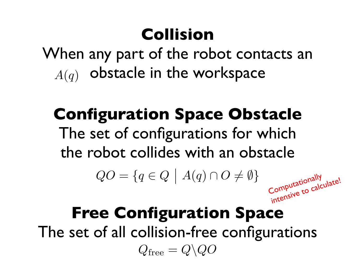
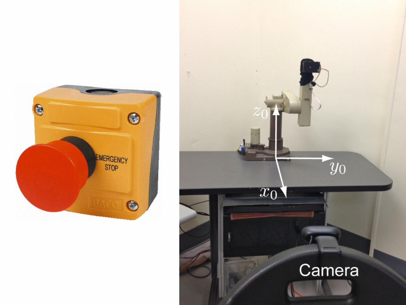
CollisionWhen any part of the robot contacts an

obstacle in the workspace

Configuration Space ObstacleThe set of configurations for whichthe robot collides with an obstacle

Free Configuration SpaceThe set of all collision-free configurations

Computationally

intensive to calculate!

Workspace Obstacles

What does the free configuration space look like for this round

mobile robot (planar PP) with one small obstacle in the workspace?

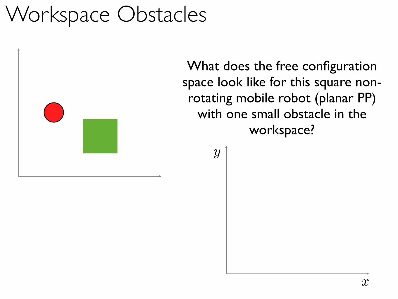
Workspace Obstacles

What does the free configuration space look like for this square non-rotating mobile robot (planar PP)

with one small obstacle in the workspace?

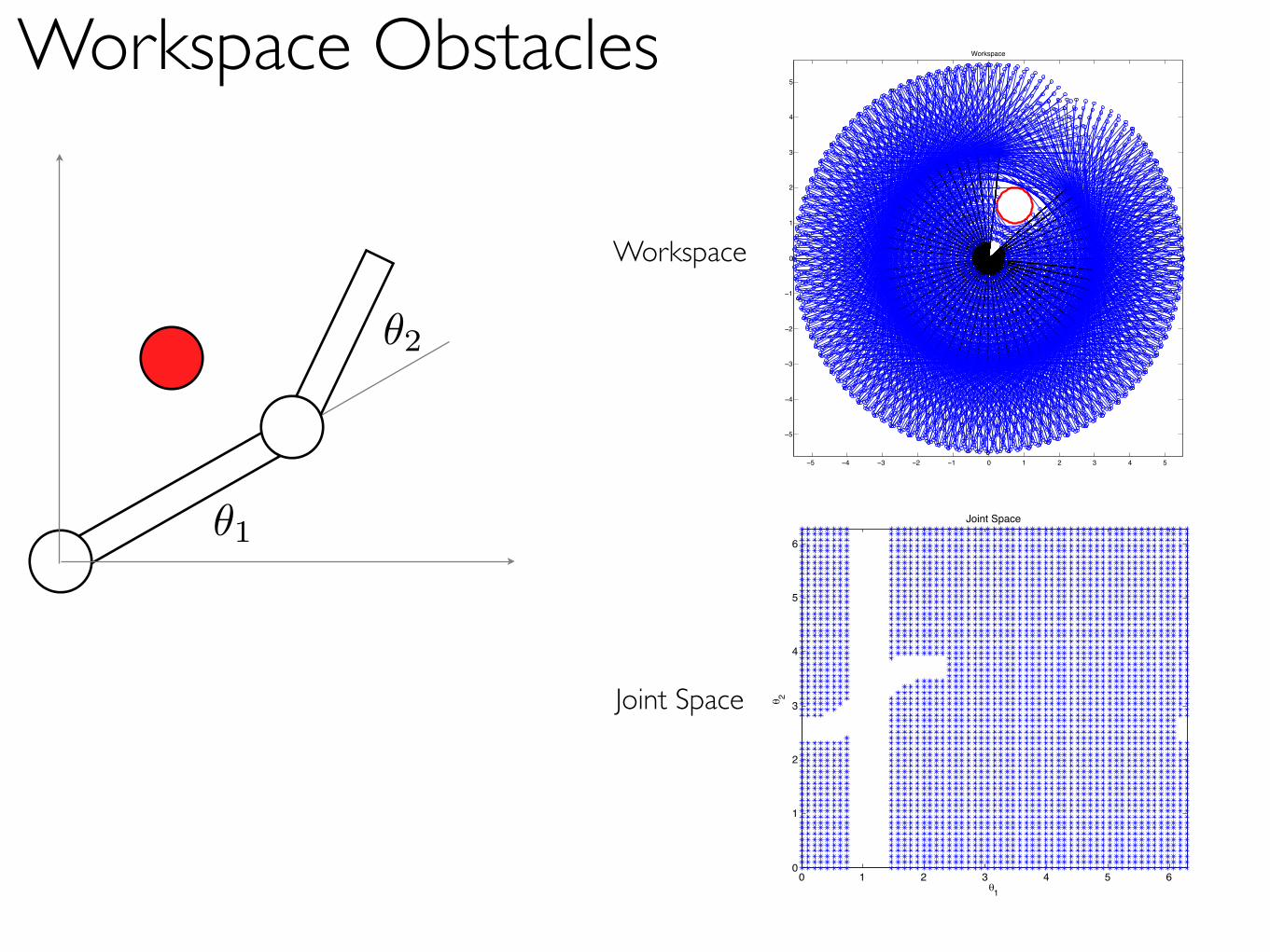
Workspace Obstacles

θ1

θ2

What does the free configuration space look like for this planar RR

manipulator with one small obstacle in the workspace?

MATLAB simulation!

Workspace Obstacles

θ1

θ2

−5 −4 −3 −2 −1 0 1 2 3 4 5

−5

−4

−3

−2

−1

0

1

2

3

4

5

Workspace

Workspace

0 1 2 3 4 5 60

1

2

3

4

5

6

θ1

θ 2

Joint Space

Joint Space

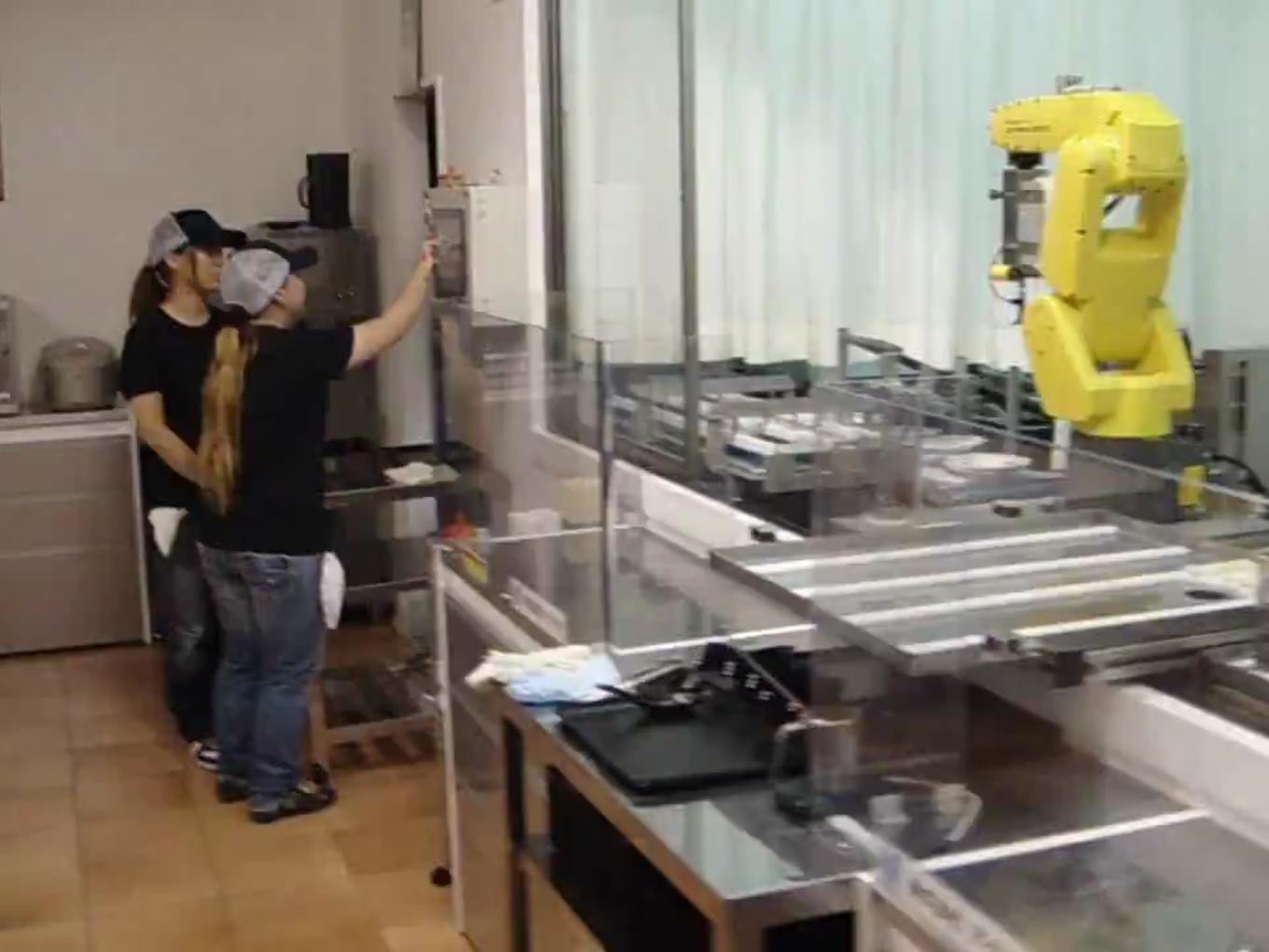
How do we prevent our robotfrom colliding with things?

Artificial Potential Fields

Treat robot as a point particle in the configuration space.

Robot feels forces from an artificial potential field U defined across its configuration space.

We design U to attract the robot to the desired final configuration and repel it from the boundaries

of obstacles.

Want one global minimum at goal with no local minima. This is often really difficult to construct!

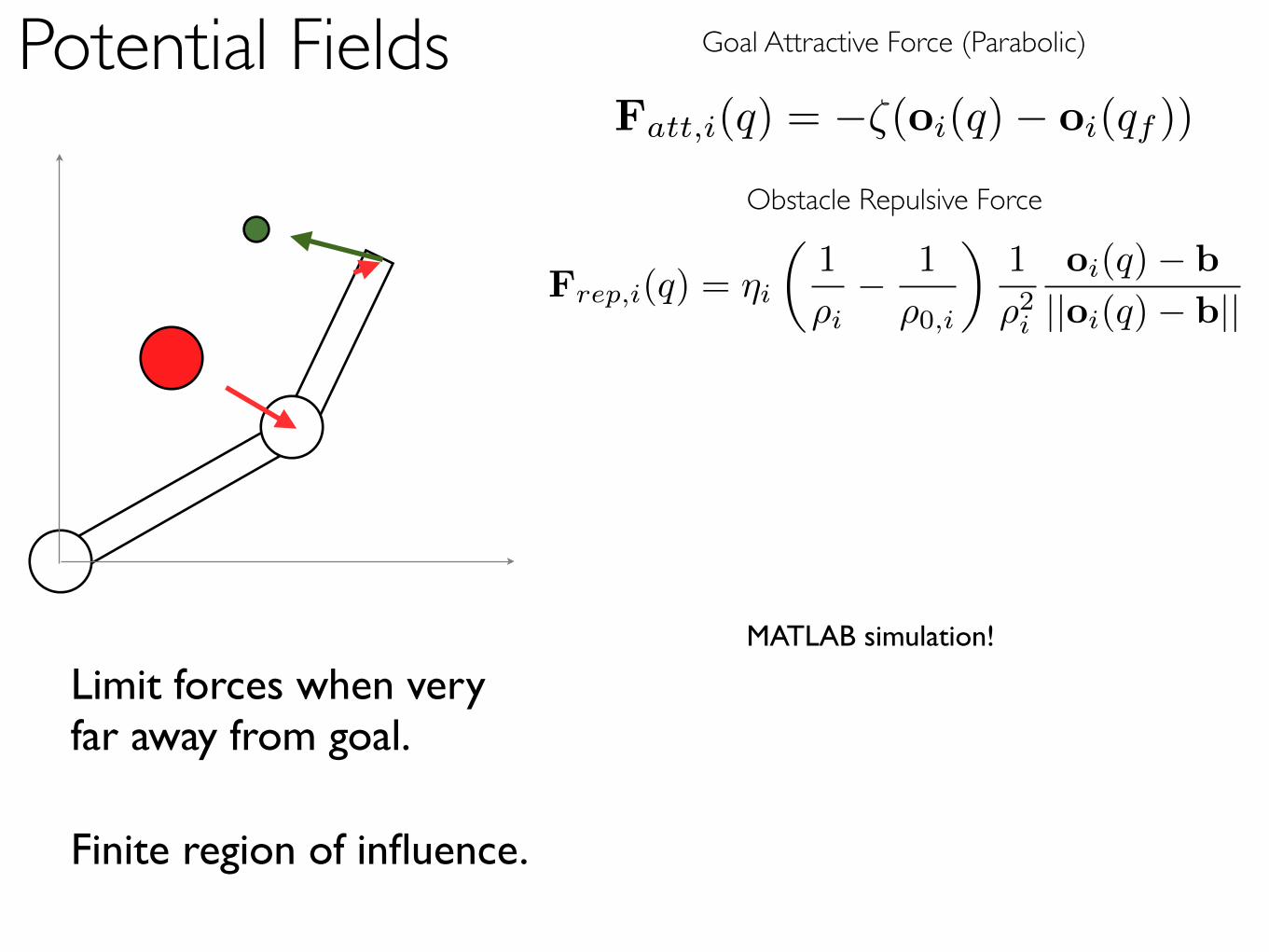
Potential Fields Goal Attractive Force (Parabolic)

Obstacle Repulsive Force

Fatt,i(q) = −ζ(oi(q)− oi(qf ))

Frep,i(q) = ηi

�1

ρi− 1

ρ0,i

�1

ρ2i

oi(q)− b

||oi(q)− b||

Limit forces when very far away from goal.

Finite region of influence.

MATLAB simulation!

Potential Fields Goal Attractive Force (Parabolic)

Obstacle Repulsive Force

Fatt,i(q) = −ζ(oi(q)− oi(qf ))

Frep,i(q) = ηi

�1

ρi− 1

ρ0,i

�1

ρ2i

oi(q)− b

||oi(q)− b||

0 1 2 3 4 5 6 7 8 9

0

1

2

3

4

5

6

7

8

Limit forces when very far away from goal.

Finite region of influence.

How do we apply these forces to the robot?

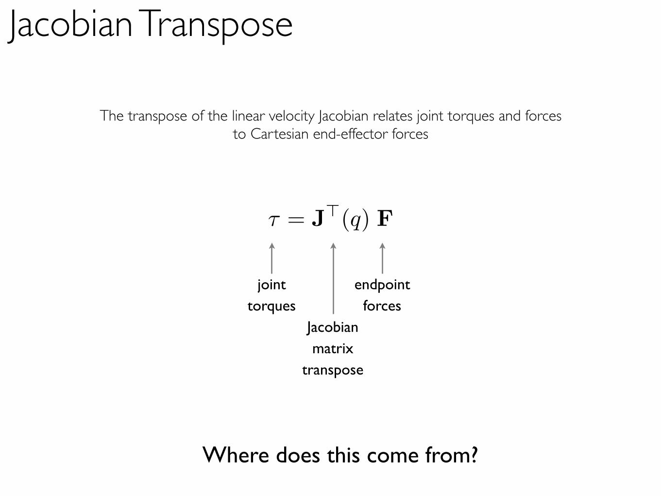
The transpose of the linear velocity Jacobian relates joint torques and forces to Cartesian end-effector forces

τ = J!(q) F

endpointforces

jointtorques

Jacobianmatrix

transpose

Jacobian Transpose

Where does this come from?

Principle of Virtual Work

Beginning with the standard Jacobian

J =

[

−a1s1 − a2s12 −a2s12

a1c1 + a2c12 a2c12

]

[

τ1

τ2

]

=

[

−a1s1 − a2s12 a1c1 + a2c12

−a2s12 a2c12

] [

Fx

Fy

]

τ = J!(q) F

We can solve for the joint torques necessary to exert a desired force at the end effector using

the Jacobian transposea1

a2

θ1

θ2

(x, y)

This is really useful!

Chapter 5 goes into more detail on potential fields and then explainsprobabilistic road maps and

trajectory planning.

Who is interested in these topics?