robotic assembly line design with tool … · robotic assembly line design with tool changes a...
TRANSCRIPT

ROBOTIC ASSEMBLY LINE DESIGN WITHTOOL CHANGES
a thesis
submitted to the department of industrial engineering
and the institute of engineering and science
of bilkent university
in partial fulfillment of the requirements
for the degree of
master of science
By
Adnan Tula
July, 2009
I certify that I have read this thesis and that in my opinion it is fully adequate,
in scope and in quality, as a thesis for the degree of Master of Science.
Prof. Dr. M. Selim Akturk (Advisor)
I certify that I have read this thesis and that in my opinion it is fully adequate,
in scope and in quality, as a thesis for the degree of Master of Science.
Prof. Dr. Erdal Erel
I certify that I have read this thesis and that in my opinion it is fully adequate,
in scope and in quality, as a thesis for the degree of Master of Science.
Assoc. Prof. Dr. Oya Ekin Karasan
Approved for the Institute of Engineering and Science:
Prof. Dr. Mehmet B. BarayDirector of the Institute
ii
ABSTRACT
ROBOTIC ASSEMBLY LINE DESIGN WITH TOOLCHANGES
Adnan Tula
M.S. in Industrial Engineering
Supervisor: Prof. Dr. M. Selim Akturk
July, 2009
This thesis is focused on assembly line design problems in robotic cells. The
mixed-model assembly line design problem that we study has several subprob-
lems such as allocating operations to the stations in the robotic cell and satisfying
the demand and cycle time within a desired interval for each model to be pro-
duced. We also ensure that assignability, precedence and tool life constraints are
met. The existing studies in the literature overlook the limited lives of tools that
are used for production in the assembly lines. Furthermore, the studies in the
literature do not consider the unavailability periods of the assembly lines and
assume that assembly lines work 24 hours a day continuously. In this study, we
consider limited lives for the tools and hence we handle tool change decisions. In
order to reflect a more realistic production environment, we deal with designing
a mixed-model assembly line that works 24 hours a day in three 8-hour shifts
and we consider lunch and tea breaks that are present in each shift. This study
is the first one to propose using such breaks as tool change periods and hence
eliminate tool change related line stoppages. In this setting, we determine the
number of stations, operation allocations and tool change decisions jointly. We
provide a heuristic algorithm for our problem and test the performances of our
heuristic algorithm and DICOPT and CPLEX solvers included in GAMS software
on different instances with varying problem parameters.
Keywords: Robotic cell, assembly line, tool change, heuristic algorithm.
iii

OZET
UC DEGISIMLI ROBOTIK MONTAJ HATTI TASARIMI
Adnan Tula
Endustri Muhendisligi, Yuksek Lisans
Tez Yoneticisi: Prof. Dr. M. Selim Akturk
Temmuz, 2009
Bu tezin konusu robotik hucrelerde montaj hattı tasarım problemleridir.
Calıstıgımız montaj hattı tasarım problemi operasyonların istasyonlara atan-
ması ve uretilecek her model icin talep ve cevrim zamanının belli aralıklar
icinde karsılanması gibi alt problemler icermektedir. Bunun yanı sıra atan-
abilirlik, oncelik ve uc omru kısıtları saglanmaktadır. Literaturde var olan
calısmalarda, montaj hatlarında uretim icin kullanılan ucların kısıtlı omru oldugu
gozardı edilmistir. Ayrıca, literaturde yer alan calısmalar 24 saat kesintisiz
uretimi temel almakta ve montaj hatlarında uretim yapılamayan zamanlar hesaba
katılmamaktadır. Bu tezde, kısıtlı uc omurleri kullanılmakta, dolayısıyla uc
degisim kararları da ele alınmaktadır. Daha gercekci bir uretim ortamı yansıtmak
amacıyla, karma model uretimi yapılan, icinde cay ve yemek molalarının oldugu
8 saatlik uc vardiya duzeniyle gunde 24 saat calısan bir montaj hattı tasarım
problemi ele alınmıstır. Bu calısma, cay ve yemek molalarının uc degistirme
zamanı olarak kullanılmasını ve bunun sonucunda uc degisim zorunlulugundan
kaynaklanan uretim hattı durdurmalarının onlenmesini onermesi acısından ilk-
tir. Bu baglamda, istasyon sayıları, operasyonların istasyonlara atanması ve uc
degisim kararları birlikte ele alınmaktadır. Calısılan problem icin cozum yolu
olarak bir sezgisel algoritma gelistirilmis, degisken degerlerin atandıgı parame-
trelerle olusturulan degisik ornekler uzerinde sezgisel algoritma ile DICOPT ve
CPLEX cozuculerinin performansları karsılastırmalı olarak test edilmistir.
Anahtar sozcukler : Robotik hucre, montaj hattı, uc degisimi, sezgisel algoritma.
iv

To my father...
v

Acknowledgement
First and foremost, I would like to express my gratitude to my advisor, Prof. Dr.
M. Selim Akturk, for his invaluable guidance and helps during my M.S. study.
With his support and advices, he has always been more than an advisor to me.
I am also grateful to Prof. Dr. Erdal Erel and Assoc. Prof. Dr. Oya Ekin
Karasan for accepting to read and review this thesis and for their invaluable
suggestions.
I would like to express my deepest gratitude to my father, Huseyin Tula and
my mother, Necla Tula for their endless love, encouragement and support. I have
always felt very lucky that I am their child, and I will always do my best to keep
them feeling the same for me.
I am indebted to all my friends who were always with me and made my life
more beautiful. I am especially grateful to Ihsan Yanıkoglu, Utku Guruscu, Konul
Bayramoglu, Safa Onur Bingol, Merve Celen, Onur Ozkok, Sibel Alumur, Duygu
Tutal, Ezel Ezgi Budak and Ceyda Kırıkcı for everything they have done for me.
Finally, I would like to express my special thanks to TUBITAK for the schol-
arship provided throughout the thesis study. The research was partially sup-
ported by Tofas Turk Otomobil Fabrikası A.S. (Fiat Turkey) as Bilkent Univer-
sity Project No: 300 189 2 5.
vi

Contents
1 Introduction 1
1.1 Literature Review . . . . . . . . . . . . . . . . . . . . . . . . . . . 2
1.2 Thesis Overview . . . . . . . . . . . . . . . . . . . . . . . . . . . . 5
2 Problem Definition 8
3 Linearization of NLMIP 18
4 Proposed Heuristic Algorithm 23
4.1 Heuristic For Finding Feasible Solutions . . . . . . . . . . . . . . 26
4.2 Improvement Algorithm . . . . . . . . . . . . . . . . . . . . . . . 31
5 Implementation 36
6 Computational Study 42
7 Conclusion 53
A Nomenclature 59
vii

List of Figures
2.1 A spot weld scheme of an automotive body component . . . . . . 9
2.2 Cycle time - revenue contribution relationship . . . . . . . . . . . 11
2.3 A spot welding gun . . . . . . . . . . . . . . . . . . . . . . . . . . 13
4.1 Cost and Profit Values for Example 1 . . . . . . . . . . . . . . . . 26
4.2 Cost and Profit Values for Example 2 . . . . . . . . . . . . . . . . 30
5.1 Tool change schedules for spot welding tools . . . . . . . . . . . . 37
5.2 Tooling Cost Calculations . . . . . . . . . . . . . . . . . . . . . . 39
5.3 Summary of spot welding tool changes . . . . . . . . . . . . . . . 40
5.4 A monitoring of shift-based tool changes . . . . . . . . . . . . . . 41
viii

List of Tables
4.1 Precedence matrix for Example 1 . . . . . . . . . . . . . . . . . . 25
4.2 Precedence matrix for Example 3 . . . . . . . . . . . . . . . . . . 34
6.1 Precedence matrix for computational study runs . . . . . . . . . . 44
6.2 Total Profit Values for Algorithm 1 and Algorithm 2 . . . . . . . 45
6.3 Calculation of Total Profit Values for Algorithm 1 and Algorithm 2 46
6.4 Total Profit Values for DICOPT 1 and MIP 1 . . . . . . . . . . . 47
6.5 Total Profit Values for DICOPT 2 and MIP 2 . . . . . . . . . . . 48
6.6 Gap values for MIP 1 and MIP 2 . . . . . . . . . . . . . . . . . . 49
6.7 Total Profit Values and CPU Times for CPLEX and Algorithm 2 50
6.8 Solution Analysis for Problem Clusters . . . . . . . . . . . . . . . 51
ix

Chapter 1
Introduction
An important application of robots in the automotive industry is their use for
spot welding operations in robotic cells. Once an automotive component of a
vehicle is designed and the required spot welds to assemble the pieces on this
component are determined, the problem of allocating the welding operations to
robotic cell stations arises. Different allocations result in different production
quantities (e.g., cycle times), station investment costs and tooling costs that
are incurred by replacing the tools with new ones. Each station consists of a
single robot in a fully automated production line. In order to perform welding
operations, the robots use spot welding guns that we refer to as welding tools
throughout this study. A welding tool has a limited life time that is represented
by the total number of spot welds that it can process.
This study focuses on a robotic cell mixed-model assembly line design problem
in which multiple models can be produced in any order. Our objective is to maxi-
mize the total profit that will be gained from the assembly line by manufacturing
automotive body components. The problem has several subproblems which in-
clude allocation of welding operations to the stations, satisfying the demand and
cycle time within a desired interval for the parts to be produced. While defining
the problem and constraints, we were inspired by a real-life assembly line problem
we faced in a project that we formerly conducted at one of the leading companies
in the automotive industry in Turkey.
1

CHAPTER 1. INTRODUCTION 2
Today, improvements in technology and automation and large investment
costs incurred for building assembly lines have increased the importance of studies
on designing efficient assembly lines. Assembly line designing problems attract
much attention from the academic world. Therefore, numerous studies have been
conducted by the researchers, in which some aspects such as equipment selection
and balancing of the lines are considered.
1.1 Literature Review
As described by Baybars [3], there are two main groups of assembly line studies.
Simple assembly line balancing problems (SALBP) consider a single product to
be produced in the assembly lines. In the literature, the widely used objectives
for these studies include minimizing the number of workstations or the cost for
building assembly lines for a given cycle time and minimizing the cycle time for a
given number of workstations. There are many studies in the field of SALB, some
of which are Baybars [2], McMullen and Tarasewich [16], Fleszar and Hindi [10],
Rekiek et al. [19], Scholl and Klein [22] and Levitin et al. [14]. For a review of
studies in the SALB field, we can refer to the review paper of Scholl and Becker
[21].
In general assembly line balancing problems (GALBP), SALB problems are
extended by introducing other aspects such as mixed-model or multi-model cases,
zoning constraints and parallel stations. As described by Becker and Scholl [4],
in a mixed-model line, different models are produced in the assembly line in an
arbitrary inter-mixed sequence. There are several studies in the literature for the
version of assembly line balancing problem with mixed-model lines. Bukchin et
al. [5] address the problem of designing mixed-model assembly lines in which a
make-to-order policy is followed. By separating the assembly tasks into two sets,
they propose a three-stage heuristic in order to find a solution with the minimum
number of stations for a given cycle time: in the first stage, they assign the first
set of tasks that should be assigned to the same station for each model requiring
these tasks. Then, they assign the second set of tasks that can be assigned to

CHAPTER 1. INTRODUCTION 3
different stations for different models to balance each model in the assembly line,
subject to the constraints resulting from the assignment of the first set of tasks.
The final stage is to improve the solution by a neighborhood search. Erel and
Gokcen [7] use a shortest-route formulation to solve a mixed-model assembly
line problem. Common assembly tasks between different models are assigned to
the same station. They transform the problem into a single-model version by
constructing a combined precedence diagram from the precedence diagrams of
all models. Bukchin and Rabinowitch [6] relax the assumption of restricting a
task that is common for several models to a particular station and allow such a
task to be assigned to different stations for different models. They provide an
integer formulation for their model and give a lower bound for the total station
cost and task assignment costs, which they aim to minimize. In order to find
optimal or near-optimal solutions, they propose a heuristic algorithm based on
branch-and-bound. Haq et al. [12] present a hybrid genetic algorithm for the
mixed-model assembly line balancing problem. They use the modified ranked
positional weight method to obtain an initial assignment of tasks to stations.
They reduce the search space and search time of their hybrid genetic algorithm
by providing this initial solution to their algorithm. Different from the studies
that adapt a single station at each stage of the assembly line, Askin and Zhou [1]
proposed a nonlinear integer program for assigning tasks to stations in a serial
line in which the stages of the assembly line consist of an arbitrary number of
identical, parallel workstations. While considering precedence relations between
tasks, they allow tooling selections for workstations and each task requires a
certain type of tool. Their objective is to minimize the sum of the total fixed
cost for operating stations and the total equipment/tooling cost. Because of the
complexity of the problem, they provide an assignment heuristic for finding good
initial solutions.
To address the problem of handling model changes in mixed-model lines,
Matanachai and Yano [15] approach the mixed-model line problem with the ob-
jective of facilitating the construction of good sequences and short-term workload
stability while assigning tasks to stations. They assume predetermined cycle times
and number of stations and include additional terms in their objective function

CHAPTER 1. INTRODUCTION 4
to minimize within- and between-station processing time diversity. Maintain-
ing short-term workload stability provides robustness for daily model changes in
mixed-model lines. Merengo et al. [17] present balancing and sequencing method-
ologies for mixed-model assembly lines to minimize the number of workstations for
predetermined model cycle times, reduce work-in-process and minimize the rate of
incomplete jobs. By presenting integer programming formulations and providing
numerical results, Sawik [20] compared monolithic and hierarchical balancing and
sequencing approaches in which balancing and sequencing of mixed-model lines
are determined simultaneously and sequencing of models proceeds the balancing
of the line, respectively.
Sparling and Miltenburg [23] were the first to study the mixed-model U-line
balancing problem to minimize the number of stations in the assembly line. For
this problem, they presented a four-step approximate solution algorithm: the first
two steps transform the mixed-model problem into an equivalent single-model
problem, the third step finds the optimal workload balance for the equivalent
single-model problem and the final step transforms the balance found in the third
step into a feasible balance for the original mixed-model problem. Miltenburg [18]
extended balancing and sequencing problem to U-shape mixed-model lines in a
just-in-time environment. A nonlinear mixed-integer programming formulation
is presented to solve the balancing and sequencing problem simultaneously. Erel
et al. [8] developed a simulated annealing-based algorithm to minimize the num-
ber of stations in a U-type assembly line and tested the performance of their
proposed algorithm against optimum seeking DP and IP-based algorithms and
other heuristic procedures. In contrast to deterministic processing times, Erel et
al. [9] studied U-line balancing problem with stochastic task times. Their study
was the first one to propose a beam search-based method to minimize total ex-
pected cost, which consists of total labor cost and total expected incompletion
cost. Van Hop [13] addressed the mixed-model assembly line problem with fuzzy
processing times for the first time. A heuristic to aggregate fuzzy processing
times is proposed and the problem is transformed into a a single-model version
by using a combined precedence diagram. A heuristic is also developed to find a
solution for the fuzzy assembly line problem. Vilarinho and Simaria [24] address

CHAPTER 1. INTRODUCTION 5
some additional zoning constraints in their study for the assignment of tasks to
stations. They assume a subset of tasks that are linked and must be assigned
to the same station and subsets of incompatible tasks that should be assigned
to different stations. They also assume that some tasks can only be assigned to
particular stations. They allow parallel stations in the assembly line and present
an ant colony optimization algorithm for minimizing the number workstations for
a given cycle time. Wilhelm and Gadidov [25] devised a branch-and-cut approach
to minimize the total assembly line cost that includes station activating, machin-
ing and tooling costs considering machine capacities and available tool spaces in
the stations. Each operation requires a set of tools to be performed so tooling
requirements constitute an important part of the problem. Machine capacity is
used as an analog of cycle time restriction that appears in single-model assembly
lines.
The studies in the literature present different model formulations and propose
different solution techniques for assembly line problems with different objective
functions. However, these studies do not consider the unavailability periods of
the assembly lines and hence are based on continuous production. In addition to
this, they overlook the limited lives of the tools that are used in production. As
we will further discuss in Chapter 5, assembly lines may suffer from tool change
related line stoppages unless the limited tool lives are taken into consideration
while allocating the operations to the stations. Therefore, we consider these two
important attributes of the robotic assembly lines in addition to other well-known
constraints of the assembly line balancing problem.
1.2 Thesis Overview
Traditional assembly line design studies are generally based on the objectives
of minimizing the cycle time, the number of stations and costs for building as-
sembly lines or maximizing the efficiency of the assembly lines. In this study,
different from the studies in the literature, we address a mixed-model assembly
line problem with a profit maximization objective. We maximize the total profit

CHAPTER 1. INTRODUCTION 6
function, which is the difference between the revenue gained by manufacturing
components of the final products and the sum of the station investment costs
and tooling costs. Station investment costs include robot cost, fixture cost and
space cost and tooling costs are incurred by replacing the tools with new ones.
In addition to this, the studies in the literature do not consider the unavailability
periods of the assembly lines and assume that assembly lines work 24 hours a day
continuously. However, we deal with designing a mixed-model assembly line that
works 24 hours a day in three 8-hour shifts. We consider lunch and tea breaks to
reflect a more realistic production environment. In the literature, there are many
studies regarding tool selection and tool costs, but these studies ignore limited
tool life and incorporate the assumption that tool change is omitted throughout
the planning horizon and tooling costs are incurred once at the beginning of the
production stage. Tool life has two implications. First, tools must be changed
at the end of their tool lives and this will increase the tooling cost. Second, tool
changes may correspond to a time when the assembly line is supposed to be op-
erating and therefore may result in line stoppages. In our study, we consider that
tools have limited lives that are represented by the total number of spot welds
that they can perform. We use the lunch and tea breaks as tool change periods
by which we aim to eliminate tool change related line stoppages. At each break,
if there exist welding tools that have a remaining number of spots less than the
total number of spots that they have to perform until the next break, they should
be changed with new ones. Therefore, the tooling cost term that appears in our
objective function is a function of the total number of tools used throughout the
planning horizon.
The organization of this study is as follows: In the next chapter we will present
a nonlinear mixed-integer formulation of our assembly line design problem. In
Chapter 3, we will provide the linearized mixed-integer version of the same prob-
lem. In Chapter 4, a heuristic algorithm for finding good feasible solutions will be
developed and this heuristic algorithm will be improved by a surrogate problem.
An implementation of our study to a leading automotive company in Turkey will
be provided in Chapter 5. Numerical results and several comparisons between
our heuristic algorithm and GAMS software are given in Chapter 6. Concluding

CHAPTER 1. INTRODUCTION 7
remarks are given in Chapter 7. A summary of all the problem parameters and
decision variables is provided in the appendix.
Chapter 2
Problem Definition
In this chapter, we give the definition of our problem and introduce the parame-
ters, variables and the mathematical model we will use to solve our problem.
We consider a robotic cell that contains at most m stations: S1, S2, . . . , Sm.
Let M={1, 2,. . . , m} be the set of indices of these stations. Space restrictions
in the production area and a limited budget for investment costs are among the
reasons of such a restriction on the number of stations. We use the parameter
Vj to denote the cost of setting up station j, j ∈ M . The cost of setting up a
station consists of robot cost, fixture cost and space cost. There are g different
models of parts to be produced in this robotic cell and G={1, 2,. . . , g} is the
index set of part models. Ohi represents operation i of model h, i ∈ Nh, h ∈ G,
where Nh={1, 2,. . . , nh} is the index set of welding operations of model h to
be allocated to stations and nh is the number of operations to be performed to
produce a part of model h. Welding operations consist of a number of spot welds.
Let Whi be the number of spot welds required to perform operation i of model
h, i ∈ Nh, h ∈ G. An operation may require a single spot weld. However, some
operations require more than one spot weld in order to assemble the part at its
proper geometry. In general, the spot welds that are close to each other with
respect to their locations on the component are grouped together as operations.
A welding tool has a limited lifetime that is represented by the total number of
spot welds it can process. We define Bj as the total number of spot welds such
8

CHAPTER 2. PROBLEM DEFINITION 9
that the welding tool in station j ∈M can process.
Figure 2.1: A spot weld scheme of an automotive body component
An example of an automotive body component is given in Figure 2.1. Figure
2.1 shows the spot welds required to perform some of the welding operations on
different locations of a part. The 26 spot welds seen in this figure constitute a
subset of all operations required to produce this body component. As we can see,
a spot weld can be close to some spot welds but can also be distant from some
other spot welds. Therefore, the locations of the spot welds on a part along with
the minimum number of required spot welds to assemble the subcomponents to
maintain their proper geometry during the part transfer between stations play
an important role in grouping these spot welds as operations.

CHAPTER 2. PROBLEM DEFINITION 10
In order to set up a profitable assembly line and determine the number of
stations required in the assembly line, we have to take the expected demand
into consideration. We represent the yearly expected demand for the parts to
be produced as θh, h ∈ G. We use the parameter γh to denote the target cycle
time for model h to meet the yearly expected demand θh. In general, let Th be
the time allocated to production of model h. Let fh be the cycle time of model
h and let θh be the corresponding production amount for model h. Then, the
relationship between fh and θh is as follows:
θh =Th
fh∀h.
We use the parameters γLh and γUh as the lower and upper bounds for the actual
cycle time of model h, respectively. We neither accept to produce an amount of
parts of model h less than the amount that can be produced when the actual cycle
time is equal to γUh nor can make any additional profit if production of model h
exceeds the amount that can be produced when the actual cycle time is equal
to γLh . Up to the production amount of θh we assume a constant profit for each
part of model h produced and denote it by PRh. In case of producing between
θh and the amount that can be produced when the actual cycle time is equal to
γLh , each excess part of model h produced contributes an expected profit denoted
by PRǫh. If the production of model h exceeds the amount that can be produced
when the actual cycle time is equal to γLh , any excess part does not contribute
any additional profit. We represent the relationship between PRh and PRǫh as
the following:
PRǫh = PRh −∆h, ∆h ≥ 0.
Let fh be the cycle time of model h for a particular allocation. Let θh and θLh
be the production amounts of model h when the cycle time of model h is equal
to the decision variable, fh, and the given parameter, γLh , respectively. In this
setting, revenue contribution of each model h, which is the sum of the individual
profits that each product of model h contributes, is calculated as in the following:
Total Revenue =
θh · PRh if γh ≤ fh ≤ γUh ,
θh · PRh + (θh − θh) · PRǫh if γLh ≤ fh ≤ γh,
θh · PRh + (θLh − θh) · PRǫh if fh < γLh .

CHAPTER 2. PROBLEM DEFINITION 11
Figure 2.2 shows an example of the relationship between the revenue contri-
bution such that PRh = $20 and PRǫh = $5 and the cycle time for a particular
model h that is produced in the assembly line, where γUh = 84 seconds, γh = 72
seconds and γLh = 64 seconds.
Figure 2.2: Cycle time - revenue contribution relationship
As we see in Figure 2.2, while the cycle time of model h decreases from γUh
(i.e., 84 seconds) to γh (i.e., 72 seconds), the contribution of model h to the total
revenue increases with a slope of PRh. While the cycle time decreases from γh
to γLh (i.e., 64 seconds), the revenue increases with a slope of PRǫh. The slope
between γh and γLh is lower than the slope between γUh and γh because after the
production amount of the expected demand θh, each excess component of model
h produced contributes an expected profit of PRǫh, which is lower than PRh.
Finally, when the cycle time decreases down from γLh , the revenue contribution of
model h remains constant because after the production amount of θLh , any excess
component of model h does not contribute any profit.
There are several reasons for an assembly line to stop when it is supposed
to be operating. For instance, the tips of the welding tools may cling on the
part during a welding operation and the welding tool then must be replaced
with a new one. Also, the grippers used for transportation of parts through the
assembly line may not close properly and therefore may not hold the part, which
causes the assembly line to stop. Moreover, the censors may not recognize or may
miscognize a part. In addition to these, a welding tool may finish its lifetime at
some time when the assembly line is supposed to be operating. Except in the

CHAPTER 2. PROBLEM DEFINITION 12
last instance, the reasons that cause the assembly line to stop are more technical
and may happen at any time. However, the last instance can be prevented by
making it possible to allow tool changes only in scheduled breaks such as tea or
lunch breaks in which the assembly line does not operate.
In most of the automotive industries (including the one that we have been
collaborating), plants work 24 hours in three 8-hour shifts and there are breaks
in an 8-hour shift. In general, there is a 10-minute break at the beginning of a
shift, a 10-minute tea break, a 30-minute lunch break and a second 10-minute
tea break. The working hours between two breaks are equal and last 1 hour and
45 minutes. Each break corresponds to a possible tool change time period. In
any break, if the remaining number of spots such that a welding tool can perform
is less than the total number of spots it has to perform until the next break, it
needs to be replaced with a new tool in that particular tool change time period
in order to prevent line stoppages due to the tool changes. Let Cj be the cost of
the tool in station j, j ∈ M . We define Dq as the available tool change time in
tool change period q, q = 1, 2, . . . , U , where U is the total number of breaks in
the planning horizon.
We calculate the required tool change time as a function of the number of
tools to be replaced:
K + µ ·
m∑
j=1
zjq ∀q = 1, 2, . . . , U,
where K is a constant that denotes the time to prepare for welding tool changes
and µ is another constant that corresponds to the time required to replace a single
welding tool. Furthermore, zjq is a binary variable to indicate whether tool in
station j ∈ M is changed in tool change period q. Two spot welding tools are
attached to the spot welding gun as shown in Figure 2.3, and both of them are
replaced at the same time.
As we have previously seen in Figure 2.1, the positions of spot welds on a
part are at different locations. It may not be possible for a particular type of
welding tool to reach to every location on a part due to its geometry. Therefore,
it is not possible to process all spot welds by one type of welding tool so there

CHAPTER 2. PROBLEM DEFINITION 13
Figure 2.3: A spot welding gun
are several types of welding tools. As a result, a welding tool cannot perform all
operations so we define an assignability matrix A and use the following parameter:
ahij =
1, if operation i ∈ Nh of model h ∈ G can be assigned
to station j ∈ M ;
0, otherwise.
There may be additional subcomponents to be assembled to a part of model
h inside the robotic cell. The subcomponents may block the positions of some
spot welds required for an operation, i.e., Ohi. Therefore, Ohi must be performed
before this particular subcomponent is assembled to the part. For similar reasons,
we define a precedence matrix P and use the following parameter:
phik =
1, if operation i ∈ Nh of model h ∈ G precedes operation
k ∈ Nh of model h ∈ G;
0, otherwise.
The difference between the processing time of a spot weld by two different
types of welding tools is negligible so the processing time of an operation is
independent of the station at which it is processed. Therefore, we let thi be the
time required to perform operation i ∈ N of model h ∈ G. We calculate thi as a
function of the number of spot welds required to perform operation i of model h

CHAPTER 2. PROBLEM DEFINITION 14
as follows:
thi = α + β ·Whi ∀h ∈ G, i ∈ Nh,
where α is a constant that denotes the time required for the robot to reach to
the position to perform operation i of model h and β is another constant that
corresponds to the time required to process a single spot weld.
In order to calculate the time allocated for production of parts of a particular
model, we need to calculate the proportion of time that should be allocated to
the production of a particular model. Therefore we define the parameter ψh for
h = 1, . . . , g as the following:
ψh =θh · γh∑g
l=1 θl · γl∀h ∈ G.
As mentioned before, the production time between two breaks is 1 hour 45 min-
utes, which is equal to 6300 seconds. Then, the time allocated for the production
of parts of model h between two breaks in the assembly line is calculated as
6300 · ψh seconds.
The decision variables we will use to formulate our model are defined below:
fh: actual cycle time for model h, h ∈ G.
σj =
{1, if station j ∈M is used in the assembly line;
0, otherwise.
xhij =
{1, if operation i ∈ Nh of model h ∈ G is assigned to station j ∈M ;
0, otherwise.
zjq =
1, if tool in station j ∈M is changed in tool change period q,
q = 1, 2, . . . , U ;
0, otherwise.
Rjq: remaining number of spot welds such that the welding tool in station j can
process after tool change period q, j = 1, 2, . . . , m, q = 1, 2, . . . , U .
CHAPTER 2. PROBLEM DEFINITION 15
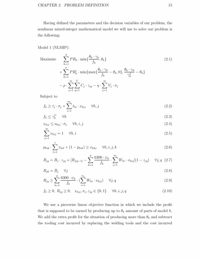
Having defined the parameters and the decision variables of our problem, the
nonlinear mixed-integer mathematical model we will use to solve our problem is
the following:
Model 1 (NLMIP):
Maximize
g∑
h=1
PRh ·min{θh · γhfh
, θh} (2.1)
+
g∑
h=1
PRǫh ·min{max{
θh · γhfh
− θh, 0},θh · γhγLh
− θh}
− ρ ·m∑
j=1
U∑
q=1
Cj · zjq − η ·m∑
j=1
Vj · σj
Subject to
fh ≥ τj · σj +
nh∑
i=1
thi · xhij ∀h, j (2.2)
fh ≤ γUh ∀h (2.3)
xhij ≤ ahij · σj ∀h, i, j (2.4)m∑
j=1
xhij = 1 ∀h, i (2.5)
phik ·
j∑
l=1
xhil + (1− phik) ≥ xhkj ∀h, i, j, k (2.6)
Rjq = Bj · zjq + [Rj(q−1) −
g∑
h=1
6300 · ψhfh
·
nh∑
i=1
Whi · xhij](1− zjq) ∀j, q (2.7)
Rj0 = Bj ∀j (2.8)
Rjq ≥
g∑
h=1
6300 · ψhfh
· (
nh∑
i=1
Whi · xhij) ∀j, q (2.9)
fh ≥ 0, Rjq ≥ 0, xhij , σj , zjq ∈ {0, 1} ∀h, i, j, q (2.10)
We use a piecewise linear objective function in which we include the profit
that is supposed to be earned by producing up to θh amount of parts of model h.
We add the extra profit for the situation of producing more than θh and subtract
the tooling cost incurred by replacing the welding tools and the cost incurred

CHAPTER 2. PROBLEM DEFINITION 16
by setting up required stations. Tooling cost and station cost are converted to
yearly costs by the constants ρ and η, which depend on the selection of U and
the number of months that the production of the selected models will continue,
respectively. Constraint (2.2) ensures that the cycle time is the maximum station
time, which is the sum of the operation times allocated to that station plus a
constant τj required for the robot in station j to begin and finalize processing
the allocated operations. By (2.3), we prevent the actual cycle time for model h
from exceeding γUh . Constraint (2.4) restricts operations to be assigned only to
the stations where they can be performed and to stations which are used in the
assembly line. By (2.5), we ensure that an operation is assigned to exactly one
station and none of the operations remains unassigned. Constraint (2.6) allows
an operation to be assigned to a station if all its predecessor operations are
assigned to the same or to a preceding station. Constraint (2.7) handles updates
for the remaining number of spot welds for welding tools in stations through the
production time. In Constraint (2.8), we define the remaining tool life for each
tool at the beginning of the planning period. In this study, we assume that we
always start the production with new tools. By constraint (2.9), we guarantee
that none of the welding tools finishes its lifetime between two breaks since the
cost of stopping the assembly line except the scheduled breaks is very costly.
In our problem, we assume that we have enough workforce to handle any
number of tool changes in a particular tool change time period. In some cases,
there may be restricted workforce to handle tool changes. Then, the following
constraint, which ensures that we do not spend more than available time for tool
changes in a particular tool change time period, can be added to Model 1:
K + µ ·m∑
j=1
zjq ≤ Dq ∀q = 1, 2, . . . , U.
In this chapter, we have defined our problem, the problem parameters and the
decision variables and formulated our problem as an NLMIP. In order to solve the
NLMIP formulation of our problem, we use DICOPT, a nonlinear solver included
in GAMS software. To work on more realistic instances, we provide data sets that
are close to the data set which we worked on in the project that we had formerly
conducted. However, as we will see in Chapter 6 in more detail, DICOPT fails to

CHAPTER 2. PROBLEM DEFINITION 17
find solutions for the NLMIP instances with the given data sets. Therefore, in the
next chapter of our study, we will convert NLMIP to a mixed integer problem by
doing necessary linearizations for the objective function and nonlinear constraints
and try to solve the equivalent mixed integer problem by using the commercial
CPLEX solver.

Chapter 3
Linearization of NLMIP
NLMIP is a nonlinear mixed integer model that includes products of two or more
variables. We continue our study with linearizing the objective function (e.g.,
equation (2.1)), constraint (2.2), constraint (2.3), constraint (2.7) and constraint
(2.9) of NLMIP with some well-known linearization techniques.
First, we define the variable ωh and replace it with 1fh
, which frequently occurs
in Model 1. Now the nonlinear part
g∑
h=1
PRh ·min{θh · γhfh
, θh}+
g∑
h=1
PRǫh ·min{max{
θh · γhfh
− θh, 0},θh · γhγLh
− θh}
in our piecewise linear objective function becomes
g∑
h=1
PRh ·min{θh · γh · ωh, θh}
+
g∑
h=1
PRǫh ·min{max{θh · γh · ωh − θh, 0},
θh · γhγLh
− θh}. (1∗)
Introducing new positive variables AOh, λ1h, λ
2h, BOh and a binary variable yh,
18

CHAPTER 3. LINEARIZATION OF NLMIP 19
we propose Constraints (3.1)-(3.8) for the linearization of our objective function.
AOh ≤ θh · γh · ωh ∀h ∈ G (3.1)
AOh ≤ θh ∀h ∈ G (3.2)
θh · γh · ωh − θh = λ1h − λ
2h ∀h ∈ G (3.3)
λ1h ≤M · yh ∀h ∈ G (3.4)
λ2h ≤M · (1− yh) ∀h ∈ G (3.5)
BOh ≤ λ1h ∀h ∈ G (3.6)
BOh ≤θh · γhγLh
− θh ∀h ∈ G (3.7)
ωh, AOh, BOh, λ1h, λ
2h ≥ 0, yh ∈ {0, 1} ∀h ∈ G (3.8)
Proposition 3.1. Constraints (3.1)-(3.8) correctly linearize the objective func-
tion introduced in NLMIP in Chapter 2, Equation (2.1).
Proof: First we replace min{θh ·γh ·ωh, θh} with AOh. Since we deal with a max-
imization problem, Constraints (3.1) and (3.2) are sufficient for the linearization
of the first term in (1∗). Then, we replace max{θh · γh · ωh − θh, 0} that appears
in the second term of (1∗) with λ1h. By Constraints (3.3)-(3.5), we ensure that
λ1h is positive if θh · γh · ωh − θh is positive, and 0 otherwise. Finally, we replace
min{λ1h,
θh·γh
γLh
− θh} that appears in the second term of (1∗) with BOh. Similar to
what we did for the linearization of the first term of (1∗), Constraints (3.6) and
(3.7) are sufficient for the linearization of the second term of (1∗). Hence, Con-
straints (3.1)-(3.8) correctly linearize the objective function introduced in NLMIP
in Equation (2.1). 2
The nonlinear part of our objective function now becomes
g∑
h=1
PRh ·AOh +
g∑
h=1
PRǫh · BOh.
The new objective function, which is now linear, is the following:
g∑
h=1
PRh · AOh +
g∑
h=1
PRǫh ·BOh − ρ ·
m∑
j=1
U∑
q=1
Cj · zjq − η ·m∑
j=1
Vj · σj

CHAPTER 3. LINEARIZATION OF NLMIP 20
Using ωh = 1fh
, constraint (2.2) becomes
1 ≥ τj · ωh +
nh∑
i=1
thi · xhij · ωh, ∀h, j. (2.2∗)
We define ehij = xhij · ωh, a very large number F and propose Constraints (3.9)-
(3.13) for the linearization of Constraint (2.2∗).
ehij ≤ ωh ∀h ∈ G, i ∈ Nh, j ∈M (3.9)
ehij ≤ F · xhij ∀h ∈ G, i ∈ Nh, j ∈M (3.10)
ehij ≥ ωh − F · (1− xhij) ∀h ∈ G, i ∈ Nh, j ∈M (3.11)
ehij ≥ 0 ∀h ∈ G, i ∈ Nh, j ∈M (3.12)
1 ≥ τj · ωh +
nh∑
i=1
thi · ehij ∀h ∈ G, j ∈M (3.13)
Proposition 3.2. Constraints (3.9)-(3.13) correctly linearize Constraint (2.2∗).
Proof: First we replace xhij · ωh with ehij . We also know that ωh is strictly
positive for each h ∈ G because cycle time of each model is strictly positive. So,
if xhij is equal to 1, by Constraints (3.9) and (3.11), ehij = ωh. If xhij is equal to
0, then by Constraints (3.10) and (3.12), ehij is equal to 0. So in any case, ehij is
equal to xhij · ωh. Hence, Constraints (3.9)-(3.13) correctly linearize Constraint
(2.2∗). 2
Since ωh = 1fh
, constraint (2.3) becomes
1
ωh≤ γUh , ∀h ∈ G. (2.3∗)
We linearize constraint (2.3∗) by replacing it with the following:
γUh · ωh ≥ 1 ∀h. (3.14)
As we previously defined ωh = 1fh
and ehij = xhij · ωh, constraint (2.7) becomes
Rjq = Bj · zjq +Rj(q−1) −Rj(q−1) · zjq −
g∑
h=1
6300 · ψh · (
nh∑
i=1
Whi · ehij)
+
g∑
h=1
6300 · ψh · (
nh∑
i=1
Whi · ehij · zjq) ∀j, q. (2.7∗)
CHAPTER 3. LINEARIZATION OF NLMIP 21
Now we define Ojq = Rj(q−1) · zjq and πhijq = ehij · zjq, and propose Constraints
(3.15)-(3.23) for the linearization of Constraint (2.7∗).
Ojq ≤ Rj(q−1) ∀j ∈M, q = 1, 2, . . . , U (3.15)
Ojq ≤ F · zjq ∀j ∈M, q = 1, 2, . . . , U (3.16)
Ojq ≥ Rj(q−1) − F · (1− zjq) ∀j ∈M, q = 1, 2, . . . , U (3.17)
Ojq ≥ 0 ∀j ∈M, q = 1, 2, . . . , U (3.18)
πhijq ≤ ehij ∀i ∈ Nh, j ∈M, q = 1, 2, . . . , U (3.19)
πhijq ≤ F · zjq ∀i ∈ Nh, j ∈M, q = 1, 2, . . . , U (3.20)
πhijq ≥ ehij − F · (1− zjq) ∀i ∈ Nh, j ∈M, q = 1, 2, . . . , U (3.21)
πhijq ≥ 0 ∀i ∈ Nh, j ∈M, q = 1, 2, . . . , U (3.22)
Rjq = Bj · zjq +Rj(q−1) −Ojq −
g∑
h=1
6300 · ψh · (
nh∑
i=1
Whi · ehij)+
g∑
h=1
6300 · ψh · (
nh∑
i=1
Whi · πhijq) ∀j ∈M, q = 1, 2, . . . , U (3.23)
Proposition 3.3. Constraints (3.15)-(3.23) correctly linearize Constraint (2.7∗).
Proof: First, we replace Rj(q−1) · zjq with Ojq. Similar to the linearization of
constraint (2.2∗), by constraints (3.15)-(3.18), the third term of the right-hand
side of Constraint (2.7∗), Rj(q−1) · zjq, becomes linear. Then, we replace ehij · zjq
that appears in the fifth term of the right-hand side of Constraint (2.7∗) with
πhijq. Similar to the linearization of Constraint (2.2∗) again, by Constraints
(3.19)-(3.22), ehij · zjq becomes linear. Hence, Constraints (3.15)-(3.23) correctly
linearize Constraint (2.7∗). 2
Using ehij = xhij · ωh again, constraint (2.9) becomes linear:
Rjq ≥
g∑
h=1
6300 · ψh · (
nh∑
i=1
Whi · ehij) ∀j ∈M, q = 1, 2, . . . , U. (3.24)
Having linearized the objective function and the necessary constraints, we finally
have the following mixed integer model:

CHAPTER 3. LINEARIZATION OF NLMIP 22
Model 2 (MIP):
Maximize
g∑
h=1
PRh · AOh +
g∑
h=1
PRǫh · BOh
− ρ ·m∑
j=1
U∑
q=1
Cj · zjq − η ·m∑
j=1
Vj · σj
Subject to Constraints (3.1)-(3.7)
Constraints (3.9)-(3.11), (3.13)
Constraint (3.14)
Constraints (2.4)-(2.6)
Constraints (3.15)-(3.17), (3.19)-(3.21), (3.23)
Constraint (2.8)
Constraint (3.24)
ωh, AOh, BOh, λ1h, λ
2h ≥ 0, yh ∈ {0, 1} ∀h, σj ∈ {0, 1} ∀j
Rjq, Ojq ≥ 0, zjq ∈ {0, 1} ∀j, q
ehij ≥ 0, xhij ∈ {0, 1} ∀h, i ∈ Nh, j, πhijq ≥ 0 ∀h, i ∈ Nh, j, q
In summary, in this chapter, we have linearized our NLMIP model and ob-
tained an MIP model by adding necessary linearization variables and constraints.
As we will see further in Chapter 6, when we try to solve MIP by using CPLEX,
we see that for several instances of MIP, CPLEX fails to find even a feasible
solution to our problem in a time limit of 2 hours. Therefore, in the next chapter
of our study, we will present a heuristic that finds a feasible solution for a given
γUh to instances of our problem. Later on, we will introduce an improvement
procedure to obtain stronger results from the given initial feasible solutions.

Chapter 4
Proposed Heuristic Algorithm
As we have mentioned before, DICOPT and CPLEX fail to solve NLMIP and
MIP instances, respectively and more detailed results for DICOPT and CPLEX
will be given in Chapter 6. Therefore, in this chapter of our study, we will first
present a heuristic algorithm that finds a set of initial feasible solutions for an
instance of our problem. In the latter step, by adding a surrogate problem to our
heuristic, we will improve the initial solutions in terms of the Total Profit value.
The heuristic algorithm that we will use for finding initial feasible solutions
is called Algorithm 1. Algorithm 1 performs several major iterations, which
result in distinct feasible solutions. Each major iteration starts with different
cycle time upper bound (i.e., γUh ) values. Therefore, when we run Algorithm 1,
by performing several major iterations, we perform a search for different initial
solutions corresponding to different cycle time values over the intervals [γLh , γUh ] for
h ∈ G. At each step of a major iteration, one operation is allocated to a station
and at each step, the allocation performed satisfies the assignability, cycle time,
precedence and tool life constraints.
The heuristic algorithm that we will use for improving the initial solutions is
called Algorithm 2. At the end of each major iteration of Algorithm 2, we solve
an additional mixed integer problem to improve the initial solution in terms of
the total profit value. The additional mixed integer problem that we solve in
23
CHAPTER 4. PROPOSED HEURISTIC ALGORITHM 24
Algorithm 2 is a reduced version of the MIP given in Chapter 3, in which we
replace our objective function with a surrogate one and use only the constraints
that are necessary for ensuring the feasibility of an allocation found.
By obtaining a set of feasible solutions rather than a single solution, we gain
more insight about the nonlinearity of our problem and the difficulty in solving
it. Example 1 that will provide us more clear information about these points is
solved by Algorithm 1, which we will soon present in Section 4.1.
Example 1: An automotive company is planning to set up a robotic cell assembly
line to produce body components for two different models of cars (g = 2). Next
year, the company plans to sell 150000 cars of the first model (θ1 = 150000)
and 75000 cars of the second model (θ2 = 75000). To achieve this production
amount, the company sets a target cycle time of 76 seconds for both models
(γh = 76 for h = 1, 2). In order to meet the orders received so far, a cycle
time of at most 80 seconds should be satisfied for both models (γUh = 80 for
h = 1, 2) and market research shows that the company can not sell cars more
than the amount that can be produced when the cycle time is 60 seconds for both
models (γLh = 60 for h = 1, 2). Cost analysis shows that up to the production
amount of 150000 for the first model and 75000 for the second model, each body
component produced will contribute a profit of $10 (PRh = 10 for h = 1, 2). In
case of producing more than the expected demand, each excess body component
produced will contribute an expected profit of $7 for both models (PRǫh = 7 for
h = 1, 2). In the production area, there is available space for at most ten stations
(m = 10). The cost of setting up one station in the assembly line is $192500
(Vj = 192500 for j = 1, 2, . . . , 10). The welding tools have a tool life of 3200 spot
welds (Bj = 3200 for j = 1, 2, . . . , 10) and each welding tool costs $10 (Cj = 10
for j = 1, 2, . . . , 10). Both models require 15 spot welding operations (nh = 15
for h = 1, 2) and the number of spots required to perform these operations are
10, 8, 8, 7, 10, 9, 8, 7, 10, 9, 7, 6, 13, 12 and 10, respectively. The time required
for a robot in a station to reach to the position to perform an operation, the
time required to perform a single spot weld and the time required for a robot
to begin and finalize processing the allocated operations are calculated to be 1,
2 and 3 seconds, respectively (α = 1, β = 2, τj = 3 for j = 1, 2, . . . , 10). An

CHAPTER 4. PROPOSED HEURISTIC ALGORITHM 25
operation can be allocated to any station (ahij = 1 for h = 1, 2, i = 1, 2, . . . , nh,
j = 1, 2, . . . , 10) and precedence relations between the welding operations are
given in the following table.
Table 4.1: Precedence matrix for Example 1
h i\k 1 2 3 4 5 6 7 8 9 10 11 12 13 14 151 1 0 0 0 0 1 1 1 1 0 0 0 0 0 0 01 2 0 0 0 0 1 1 1 1 0 0 0 0 0 0 01 3 0 0 0 0 1 1 1 1 0 0 0 0 0 0 01 4 0 0 0 0 1 1 1 1 0 0 0 0 0 0 01 5 0 0 0 0 0 0 0 0 1 1 1 1 0 0 01 6 0 0 0 0 0 0 0 0 1 1 1 1 0 0 01 7 0 0 0 0 0 0 0 0 1 1 1 1 0 0 01 8 0 0 0 0 0 0 0 0 1 1 1 1 0 0 01 9 0 0 0 0 0 0 0 0 0 0 0 0 1 1 11 10 0 0 0 0 0 0 0 0 0 0 0 0 1 1 11 11 0 0 0 0 0 0 0 0 0 0 0 0 1 1 11 12 0 0 0 0 0 0 0 0 0 0 0 0 1 1 11 13 0 0 0 0 0 0 0 0 0 0 0 0 0 0 01 14 0 0 0 0 0 0 0 0 0 0 0 0 0 0 01 15 0 0 0 0 0 0 0 0 0 0 0 0 0 0 02 1 0 0 0 0 1 1 1 1 0 0 0 0 0 0 02 2 0 0 0 0 1 1 1 1 0 0 0 0 0 0 02 3 0 0 0 0 1 1 1 1 0 0 0 0 0 0 02 4 0 0 0 0 1 1 1 1 0 0 0 0 0 0 02 5 0 0 0 0 0 0 0 0 1 1 1 1 0 0 02 6 0 0 0 0 0 0 0 0 1 1 1 1 0 0 02 7 0 0 0 0 0 0 0 0 1 1 1 1 0 0 02 8 0 0 0 0 0 0 0 0 1 1 1 1 0 0 02 9 0 0 0 0 0 0 0 0 0 0 0 0 1 1 12 10 0 0 0 0 0 0 0 0 0 0 0 0 1 1 12 11 0 0 0 0 0 0 0 0 0 0 0 0 1 1 12 12 0 0 0 0 0 0 0 0 0 0 0 0 1 1 12 13 0 0 0 0 0 0 0 0 0 0 0 0 0 0 02 14 0 0 0 0 0 0 0 0 0 0 0 0 0 0 02 15 0 0 0 0 0 0 0 0 0 0 0 0 0 0 0
When we solve Example 1 with Algorithm 1, we get different solutions and
objective function values corresponding to different cycle times. Figure 4.1 shows
the values for the objective function terms and the objective function value as
Total Profit for the corresponding cycle times.
As seen in Figure 4.1, revenue, which is the sum of the profits that each
product contributes, strictly increases as the cycle times decrease until to γLh

CHAPTER 4. PROPOSED HEURISTIC ALGORITHM 26
Figure 4.1: Cost and Profit Values for Example 1
values. Station cost is a nondecreasing function as long as the cycle times decrease
because lower cycle times require a larger number of stations and it exhibits a
stepping structure due to the breakpoints that correspond to particular cycle
times.
After giving an insight about the solution of our problem and the nonlinearity
of our objective function, we now present our heuristic algorithm that we use for
finding initial solutions.
4.1 Heuristic For Finding Feasible Solutions
The heuristic that we introduce in this section consists of several major iterations.
The only difference between these iterations are the values of parameter γUh , the
upper bound on the cycle time for model h, h ∈ G. Using different γUh values at
each major iteration result in a distinct feasible solution. In each major iteration,

CHAPTER 4. PROPOSED HEURISTIC ALGORITHM 27
we start with creating a list I of unassigned operations, which initially includes
all operations and becomes empty when all of the operations are allocated to the
stations. Then, by using predecessor matrix P , for each operation Ohi we create
pred(h, i), a list that includes all predecessor operations of Ohi. In the further
steps of each iteration, while allocating an operation to a station, we need to
use the original pred(h, i) lists to ensure that the allocation satisfies precedence
constraints, but we also need to update these lists whenever an operation is
allocated to a station. Therefore, for each Ohi, we create another predecessor
list pred(h, i), which is initially a copy of pred(h, i) but is subject to changes
in the further steps. The reason for keeping dynamic pred(h, i) lists is that an
operation becomes assignable when its pred(h, i) list is empty. While assigning
the operations to the stations, for each station, we need to keep information
about the total time spent and total number of spots performed for a particular
model in order to ensure that cycle time and tool life constraints remain satisfied.
Therefore, we use loadhj and spothj, which keep the necessary information about
the total time spent and total number of spots performed for a particular model
in each station and which are initially equal to τj and 0, respectively.
After these initializations, we start allocating the welding operations to sta-
tions. At each step, we allocate only one operation to a station. Therefore, we
perform∑g
h=1 nh steps until there is no operation left to allocate, in other words,
I = Ø. At each step, we choose to allocate the operation Ohi with the largest
operation time and whose predecessor operations have all been allocated before.
Our selection rule resembles using Longest Processing Time (LPT) rule, which is
one of the most popular techniques used in bin packing problems. By allocating
the operation with the largest processing time, we aim to have a solution with as
few stations as possible, in other words, with as low investment costs as possible.
We allocate such a candidate operation to the station with minimum possible
index, while ensuring the feasibility of four important constraints. Firstly, the
candidate operation should be assignable to that station. Secondly, after allocat-
ing the candidate operation, the cycle time for that particular model should not
be exceeded. Thirdly, we check if each predecessor operation of the candidate
operation has been assigned to the same or to a preceding station. Finally, we

CHAPTER 4. PROPOSED HEURISTIC ALGORITHM 28
ensure that after allocating the candidate operation, the total number of spots
that will be performed at that station between two breaks will not exceed the
life of the welding tool at the same station. Once we allocate an operation to
a station, we remove it from I, the list of unassigned operations. We update
loadhj and spothj for the station that the operation is allocated and remove the
operation from the predecessor lists pred(h, i) of those other operations for which
the allocated operation is a predecessor operation. When the allocation of all op-
erations is complete, we calculate objective function value for the corresponding
solution.
As mentioned before, our heuristic consists of several major iterations. We
start the first major iteration with γUh = γUh values for each h ∈ G. At the end of
each major iteration, we obtain cycle time (fh) values and start the next major
iteration with γUh = fh − 1. This setting provides us to obtain different solutions
from each major iteration and we continue this process until γUh < γLh for each
h ∈ G. The reason behind this stopping criterion is that achieving a cycle time
fh lower than γLh for any model does not contribute any additional profit and
therefore the objective function value does not increase.
In Example 1 that was presented at the beginning of this chapter, the largest
objective function value corresponds to the solution in which fh = γh for both
models. But since all objective function terms depend on the values of cycle
times, this may not always be the case. In other words, we may obtain larger
objective function values with arbitrary cycle times. The following example shows
the importance of why we perform a search for different solutions corresponding
to different cycle time values over the intervals [γLh , γUh ] for h ∈ G.
Example 2: Suppose that the company in Example 1 can not sell cars more
than the amount that can be produced when the cycle time is 65 seconds instead
of 60 seconds for both models (γLh = 65 for h = 1, 2). Furthermore, the cost of
setting up one station in the assembly line is decreased to $110000 (Vj = 110000
for j = 1, 2, . . . , 10) instead of $192500 in the previous example. All the data
provided in Example 1 except these two remain the same. For Example 2, Figure
4.2 shows the values for the objective function terms and the objective function

CHAPTER 4. PROPOSED HEURISTIC ALGORITHM 29
Algorithm 1: Heuristic for finding initial feasible solutionsInput: m ∈ IN, g ∈ IN, nh for h = 1, . . . , g, A, P, Whi for h = 1, . . . , g,
i = 1, . . . , nh, Bj and τj for j = 1, . . . ,m, γh, γUh and θh for h = 1, . . . , g.Output: S, a set of feasible solution(s)begin
initialize
γUh = γUh ∀h ∈ G
S = Øwhile ∃ γUh such that γUh ≥ γLh do
Create list I that contains all operations Ohi, h = 1, . . . , g, i = 1, . . . , nhCreate predecessor list pred(h, i) for each Ohi, h ∈ G, i ∈ Nh from P
initialize
pred(h, i) = pred(h, i), loadhj = τj, spothj = 0 for all h = 1, . . . , g,i = 1, . . . , nh, j = 1, . . . ,m
while I 6= Ø do
Find an operation Ohi ∈ I with pred(h, i) = Ø and maximum thiAssign Ohi to station Sj with minimum possible index such that
ahij = 1loadhi + thi ≤ γUhphik ·
∑jl=1 xhil + (1− phik) ≥ xhkj for each k ∈ pred(h, i)
6300·ψh
max{maxk∈M\j{loadhk},loadhj+thi}· (spothj + Whi)
+∑
h∈G\h
6300·ψh
maxk∈M{loadhk}· spothj ≤ Bj
loadhj = loadhj + thispothj = spothj + Whi
I = I \ {Ohi}
pred(c, d) = pred(c, d) \ {Ohi} for all Ocd ∈ I
Let y be the corresponding solutionFind ϕy, the corresponding objective function valueS = S ∪ y
fh ← maxj∈M{loadhj} ∀h ∈ G
γUh ← fh − 1 ∀h ∈ G
end

CHAPTER 4. PROPOSED HEURISTIC ALGORITHM 30
value as Total Profit for the corresponding cycle times.
Figure 4.2: Cost and Profit Values for Example 2
The two different Total Profit value patterns in Figure 4.1 and Figure 4.2 show
that our problem is difficult in the sense that Total Profit is a ‘very nonlinear
function’ according to the DICOPT solutions manual. Also, Figure 4.2 clearly
shows that there may be multiple peak points of Total Profit function, which
means that the global optimum for the objective function value may correspond to
particular cycle times in the intervals [γLh , γUh ] for h ∈ G and even for the instances
of NLMIP that can be solved by DICOPT, there is the fact that DICOPT may get
stuck in one of the local optima. Therefore, we perform a search for alternative
solutions corresponding to different cycle time values over the intervals [γLh , γUh ]
for h ∈ G. In addition to these facts, we still do not know whether we find the
best solution achievable in terms of the objective function value. Hence, in the
following section of our study, we will try to strengthen our search methods in
order to find better solutions than the ones that we can find with Algorithm 1.
CHAPTER 4. PROPOSED HEURISTIC ALGORITHM 31
4.2 Improvement Algorithm
Algorithm 1 presented in Section 4.1 does not necessarily give an optimal alloca-
tion of operations in terms of the objective function value of MIP. In other words,
there may be a better allocation of operations that corresponds to cycle times
different than the ones that correspond to a solution found by Algorithm 1.
As previously defined, let y ∈ S be a feasible solution that is found by Algo-
rithm 1 to our problem. Let my be the number of stations used in the assembly
line in the feasible solution y. As long as the cycle times are larger than the
corresponding γLh values, achieving lower cycle times with less than or equal to
my stations increases the revenue and so the Total Profit, which we aim to max-
imize. Hence, in this section, we present the following problem, in which we use
a surrogate objective function to minimize the cycle time of each model to be
produced in addition to the overall cycle time denoted by MaxCycleTime.
Minimize MaxCycleTime +
g∑
h=1
fh − γLh
Subject to MaxCycleTime ≥ fh ∀h
Constraint (2.2)
(SP)m∑
j=1
σj ≤ my
Constraints (3.9)-(3.11), (3.13), (3.14)
Constraints (2.4)-(2.6)
Bj ≥
g∑
h=1
6300 · ψh · (
nh∑
i=1
Whi · ehij) ∀j
MaxCycleTime ≥ 0, fh, ωh ≥ 0 ∀h,
ehij ≥ 0, xhij ∈ {0, 1} ∀h, i ∈ Nh, j, σj ∈ {0, 1} ∀j
In order to achieve better allocations of operations in terms of the objective
function value, we reduce our problem to SP. The optimal allocation to SP is
still a feasible solution for MIP that is presented in Chapter 3 as shown in the
following lemma.

CHAPTER 4. PROPOSED HEURISTIC ALGORITHM 32
Lemma: Let x be an optimal solution to SP, then x is a feasible solution to MIP.
Proof: In SP, we omit constraints (3.1)-(3.8), (3.15)-(3.17), (3.19)-(3.21), (3.23),
(2.8) and (3.24), which are present in MIP. We need constraints (3.1)-(3.8) for
linearization of the objective function of NLMIP. Since our objective in SP is
different from MIP, omitting these constraints does not affect the feasibility of
x to MIP. We use constraints (3.15)-(3.17), (3.19)-(3.21) and (3.23) in MIP for
linearization of constraint (2.7) in NLMIP. Together with constraints (2.8) and
(3.24), these constraints ensure that the remaining number of spot welds that a
welding tool in station j can perform after tool change time period q is greater
than or equal to the number of spot welds it has to perform until the next tool
change time period. In other words, we need these constraints to determine the
values of zjq variables, which are necessary for calculation of tooling costs in the
objective function. Again, since we have a different objective function and zjq
values are necessary for calculation of tooling costs, omitting constraints (3.15)-
(3.17), (3.19)-(3.21), (3.23), (2.8) and (3.24) does not affect the feasibility of x to
MIP. 2
Let y ∈ S be a feasible solution that is found by Algorithm 1 to our problem
and let my be the number of stations used in the assembly line in the feasible
solution y. We first run SP for my − 1 stations with the same upper bound and
other parameters used in Algorithm 1 that result in the feasible solution y. If the
same cycle times in the feasible solution y can not be met by using less number
of stations, we run SP again for my stations to improve the cycle times and so
the Total Profit that we want to maximize in the original problem.
Let y ∈ S be a feasible solution that is found by Algorithm 1 to our problem
and let y be an optimal SP solution using the same parameters that result in
the feasible solution y in Algorithm 1. Let ϕy and ϕy be the objective function
values that correspond to y and y, respectively. Algorithm 2 is a combination of
Algorithm 1 and SP.
As mentioned in the previous chapter of our study, the difficulty of our problem
results from the fact that our objective function is very nonlinear. In the following
example, we will see how DICOPT fails to find the optimal solution and how we

CHAPTER 4. PROPOSED HEURISTIC ALGORITHM 33
Algorithm 2: Algorithm for improving heuristic solutionsInput: m ∈ IN, g ∈ IN, nh for h = 1, . . . , g, A, P, Whi for h = 1, . . . , g,
i = 1, . . . , nh, Bj and τj for j = 1, . . . ,m, γh, γUh and θh for h = 1, . . . , g.Output: Best solutionbegin
initialize
γUh = γUh ∀h ∈ G
S = Ø, S = Øwhile ∃ γUh such that γUh ≥ γLh do
Create list I that contains all operations Ohi, h = 1, . . . , g, i = 1, . . . , nhCreate predecessor list pred(h, i) for each Ohi, h ∈ G, i ∈ Nh from P
initialize
pred(h, i) = pred(h, i), loadhj = τj, spothj = 0 for all h = 1, . . . , g,i = 1, . . . , nh, j = 1, . . . ,m
while I 6= Ø do
Find an operation Ohi ∈ I with pred(h, i) = Ø and maximum thiAssign Ohi to station Sj with minimum possible index such that
ahij = 1loadhi + thi ≤ γUhphik ·
∑jl=1 xhil + (1− phik) ≥ xhkj for each k ∈ pred(h, i)
6300·ψh
max{maxk∈M\j{loadhk},loadhj+thi}· (spothj + Whi)
+∑
h∈G\h
6300·ψh
maxk∈M{loadhk}· spothj ≤ Bj
loadhj = loadhj + thispothj = spothj + Whi
I = I \ {Ohi}
pred(c, d) = pred(c, d) \ {Ohi} for all Ocd ∈ I
Let y be the corresponding feasible solutionS = S ∪ y
Solve the SP model with the same parameters and find y, thecorresponding SP solutionS = S ∪ y
fh ← maxj∈M{loadhj} ∀h ∈ G
γUh ← fh − 1 ∀h ∈ G
Find ϕy and ϕy for each y ∈ S and y ∈ S
Best← argmaxy∈S,y∈S{max{maxy∈Sϕy,maxy∈Sϕy}}
end

CHAPTER 4. PROPOSED HEURISTIC ALGORITHM 34
improve our heuristic results by adding the surrogate problem.
Example 3: Suppose that the company in Example 1 has an available space
in their production area only for four stations (m = 4). Suppose further that
both models require 10 spot welding operations (nh = 10 for h = 1, 2) and the
number of spot welds required to perform these operations are 10, 8, 8, 7, 10, 9,
8, 7, 10 and 9, respectively. Except precedence relations, all the data provided
in Example 1 remain the same. Precedence relations for operations are given in
Table 4.2.
Table 4.2: Precedence matrix for Example 3
h i\k 1 2 3 4 5 6 7 8 9 101 1 0 0 0 0 1 1 1 1 0 01 2 0 0 0 0 1 1 1 1 0 01 3 0 0 0 0 1 1 1 1 0 01 4 0 0 0 0 1 1 1 1 0 01 5 0 0 0 0 0 0 0 0 1 11 6 0 0 0 0 0 0 0 0 1 11 7 0 0 0 0 0 0 0 0 1 11 8 0 0 0 0 0 0 0 0 1 11 9 0 0 0 0 0 0 0 0 0 01 10 0 0 0 0 0 0 0 0 0 02 1 0 0 0 0 1 1 1 1 0 02 2 0 0 0 0 1 1 1 1 0 02 3 0 0 0 0 1 1 1 1 0 02 4 0 0 0 0 1 1 1 1 0 02 5 0 0 0 0 0 0 0 0 1 12 6 0 0 0 0 0 0 0 0 1 12 7 0 0 0 0 0 0 0 0 1 12 8 0 0 0 0 0 0 0 0 1 12 9 0 0 0 0 0 0 0 0 0 02 10 0 0 0 0 0 0 0 0 0 0
In this example, the best objective function value that is achievable by Al-
gorithm 1 is 1640022 and in this solution, the number of stations used in the
assembly line is equal to 3 and cycle times for both models are equal to 73. How-
ever, when we run SP, we see that with 3 stations, a cycle time of 69 is achievable
for both models. Such a decrease in the cycle time results in more production
and so in more revenue. Hence, the best objective value achievable increases to
1735082 by Algorithm 2. Furthermore, the best solution found for this instance by
DICOPT has an objective function value of 1702947, which means that DICOPT

CHAPTER 4. PROPOSED HEURISTIC ALGORITHM 35
got stuck in one of the local optima of the objective function. Moreover, this
relatively small instance of our problem can be solved to optimality by CPLEX
in approximately 20 minutes and the optimal value is the same with the one that
we find by Algorithm 2. But for this instance, Algorithm 2 finds the optimal
solution just in a few seconds.
In this chapter, we have given our proposed heuristic algorithm together with
some examples and numerical results. In the next chapter, we will see an overview
of the implementation of our tool change decisions to a real-life assembly line
problem. In Chapter 6, we will test the performance of our heuristic on some
instances of our problem and compare the performances of our heuristic and
DICOPT and CPLEX solvers.

Chapter 5
Implementation
In this chapter, we will give some details about the tool change decision policy
that we proposed to solve the real-life assembly line problem that we faced in
the project that we had formerly conducted at one of the leading automotive
companies in Turkey. As mentioned before, while defining our problem and con-
straints in our study, we were inspired by this project. Our aim in the project
was to increase the efficiency of an assembly line that performed spot welding op-
erations and produced body components for different models of cars. The most
important problem of the assembly line was that some tool changes coincided to
the times when the assembly line was supposed to be operating. Therefore, in
order to perform tool changes, the assembly line was stopped and this resulted in
loss of production. In their previous assembly line balancing problems, the com-
pany has allocated almost 10% of their available capacity to the line stoppages
due to the tool changes. To eliminate such tool change related line stoppages,
we developed a decision support system that indicated at which break each of
the welding tools in the assembly line should be replaced with a new one. All
the relevant information about operation allocations, number of spot welds that
each tool must perform and cycle times for each model was provided to us by
the company. However, since the assembly line was operating for a long time,
we did not have a chance to revise the allocation of welding operations to the
stations because it would take a long time to recode the robot operations and
36

CHAPTER 5. IMPLEMENTATION 37
movements and to perform production simulation studies. Therefore, we were
able to apply the results of our tool change analysis only to the current system,
without changing any operation allocation. Figure 5.1 is a screenshot of one of
the modules that we had in our decision support system.
Figure 5.1: Tool change schedules for spot welding tools
Figure 5.1 shows a part of a weekly tool change schedule for spot welding
tools. The four buttons on the left are used for returning back to the tool change
schedule of the previous week, advancing to the next production week and forming
the tool change schedule and generating a tool change report. The dates and the
starting and ending hours of each break are given. The work duration column
shows the production time between the current break and the next break. R1,
R2, R3, R4, R5 and R6 represent the spot welding tools at six different stations.
Under these columns, the remaining life of welding tools after each break is given.
If the number ’1’ occurs in any cell of these columns, it means that the welding
tool has to be changed with a new one at the corresponding break because the
remaining life of the tool is not enough for that tool to be used for production

CHAPTER 5. IMPLEMENTATION 38
until the next break.
If the remaining life of a tool after a particular break is negative and hence
the corresponding cell is highlighted (i.e., filled in red), it means that the life of
such a tool has expired at some time before the break. Although the tool change
decisions are made to eliminate such occurrences and hence tool change related
line stoppages, it did not work for all the spot welding tools in the current sys-
tem. This might occur for two reasons. In initial allocation of the operations,
there might be some spot welding tools with a very frequent usage such that
the tool life might be shorter than the available time period. Another reason
is that our decision support system uses real time data and once it is executed,
it obtains the current time and the remaining number of spot welds that each
tool can perform from Welding Management System (WMS), version 2.94, which
is a software developed for welding operations by Gf Welding S.p.A. company.
Therefore, there might be some deviation between the actual number of compo-
nents being produced and the expected demand information that we have used
in our formulation due to the unexpected events leading to line stoppages such
as the tips of the welding tools may cling on a part during a welding operation,
the grippers used for transportation of parts through the assembly line may not
close properly or the censors may not recognize or may miscognize a part. For
example, although the welding tools R2 and R4 are changed at every break, they
still sometimes cause the assembly line to stop between two particular breaks.
The reason for such stoppages was that the number of spots that the welding
tools R2 and R4 had to perform between two particular breaks as a result of the
predetermined operation allocations sometimes exceeded their tool lives in terms
of the total number of spot welds that they can perform. Therefore, it can be
derived that tool change related stoppages in assembly lines cause from alloca-
tion of operations which are determined without considering the limited lives of
tools that are used for production. Hence, this is the reason why we determine
operation allocations and tool change decisions jointly in our study.
Another useful property of our decision support system is that one can see the
corresponding tooling cost that is incurred for particular tool change schedules.
Figure 5.2 shows the weekly and yearly tooling costs for a particular tool change

CHAPTER 5. IMPLEMENTATION 39
schedule.
Figure 5.2: Tooling Cost Calculations
The tooling cost calculations enable the company to do sensitivity analysis for
tool change decisions. As seen in Figure 5.2, in the current system, there are some
tools that are changed before the end of their tool lives (i.e., earliness > 0) and
some other tools that cause the assembly line to stop (i.e., lateness > 0). As we
have observed in the actual production, if they could have reallocated one or two
operations from station 4 to station 3 (which was feasible due to the cycle time,
precedence and assignability constraints), both the earliness cost of station 3 and
the lateness cost of station 4 could be decreased at the same time. Therefore, the
current allocation could easily be improved in terms of the tooling cost leading
to a higher total profit value since the other parameters in the objective function
remain the same. If the tool change earliness is high and the reallocation is not
possible due to either cycle time or precedence or assignability constraints, the
company may set up automated tool changers in the assembly line. If this option
is realized, there might be some loss in the total available production time due to
decreasing the earliness because the tools that are changed early will be changed
at some time when the assembly line is supposed to be operating, rather than in
breaks. However, there might also be some gain in the total available production
time due to decreasing the lateness because automated tool changers will change
the tool in relatively shorter time with respect to stopping the assembly line and
changing the tools manually. In addition to these, automated tool changers may
decrease the reliability of the tool changes and hence the quality of the products.
Moreover, investment costs will be incurred for setting up tool changers in the
assembly lines. However, increasing the utilization of the spot welding tools would
decrease the total tooling cost. Therefore, sensitivity analysis that can be handled

CHAPTER 5. IMPLEMENTATION 40
via our decision support system is very useful for evaluating such options.
In addition to providing tool change schedules, we provided a summary of
tool changes and the total number of tools to be changed at each break as a tool
change support system. Figure 5.3 shows another module of our decision support
system, which indicates necessary tool changes to be performed at each break.
Figure 5.3: Summary of spot welding tool changes
Figure 5.3 shows only the tool change times for each spot welding tool and the
total number of tools to be changed at each break. The values in the total number
of tool changes column are also used for calculating the total weekly tooling cost.
In order to send the tool change decisions to the production area, we provided
an interface to be monitored in the production area in order for the workers
to obtain necessary information for tool change schedules. Figure 5.4 shows a
shift-based summary of tool changes. Based on the current data obtained at any
time, our module determines and reports the necessary welding tool changes for
each break of the current shift. When monitored in the production area, this

CHAPTER 5. IMPLEMENTATION 41
information also provides the workers an ease for tracing and performing tool
changes.
Figure 5.4: A monitoring of shift-based tool changes

Chapter 6
Computational Study
In this chapter of our study, we will evaluate the performances of our heuris-
tic method and the commercial solvers DICOPT2X-c and CPLEX 10.1 for our
problem and provide some computational results that we obtained by using Al-
gorithm 1 and Algorithm 2 that are coded in C++ environment, and the solvers
mentioned above. We used the modeling interface of GAMS 22.3. A computer
with 1024 MB memory and Pentium Dualcore 1.73 GHZ CPU was used for taking
the runs. First of all, we define the data set that we used in our runs.
There are two important factors that affect the size of our problem and optimal
allocations in the solutions. The first one is the parameter g, the number of
different models that will be produced in the robotic cell assembly line. As this
parameter increases, our problem becomes harder to be solved by the commercial
solvers DICOPT or CPLEX. The second one is the ratio of the profit contribution
of the models to the station investment cost, denoted as PRh
Vj. This ratio is very
important to evaluate the tradeoff between the revenue and the number of stations
that will be used in the assembly line. We set two levels as low and high for both
of these factors. When the number of models is at its low level we use g = 2 and
when it is at its high level, we use g = 4. We use a constant cost of $180000 for
setting up one station in the assembly line, Vj = 180000 for j = 1, 2, . . . , m where
m is an upper bound for the number of stations. When the ratio PRh
Vjis at its
low level, PRh is a uniform random number from the interval [5,7]. When this
42

CHAPTER 6. COMPUTATIONAL STUDY 43
ratio is at its high level, the interval from which we select the values for PRh is
[9,11]. Using the combinations of these two factors at low and high level, we have
four main clusters for our runs in which these two factors have low-low, low-high,
high-low and high-high levels. We take 5 replications for each cluster so a total
of 20 different runs are taken.
The value of the parameter nh, the number of spot welding operations required
for model h, is a uniform random number from the interval [8,15]. The value of
the parameter Whi, the number of spot welds required to perform operation i
of model h, is also a uniform random number from the interval [6,15]. In all
the runs, we used m = 6 for the upper bound on the number of stations that
can be used in the assembly line. We used a constant value of 3 seconds for the
parameter τj , j = 1, . . . , 6 and a constant value of $10 for Cj, j = 1, . . . , 6 for the
cost of welding tools. The values of the parameters Bj , j = 1, . . . , 6 are uniform
random numbers from the interval [3200,4000]. We also used constant values of
1 seconds and 2 seconds for the time required for a robot in a station to reach to
the position to perform an operation and the time required to perform a single
spot weld, respectively (α = 1, β = 2).
When the number of models is at the low level, we use θ1 = 150000 and
θ2 = 75000 and at the high level, we use θ1 = 100000, θ2 = 50000, θ3 = 50000
and θ4 = 25000 for the values of expected demands. We set the value of the
expected profit for each excess production of model h as PRǫh = ⌈PRh · 0.7⌉.
In order to set the values of the cycle time lower bound (γLh ), cycle time upper
bound (γUh ) and target cycle time (γh) parameters for a particular model h, we
use the following procedure. First, we calculate thi, the average time to perform
one spot welding operation of model h. We round 3 · thi to the nearest integer
and use this value for γLh . We round 4 · thi to the nearest integer and use this
value for γUh . The value of the parameter γh is a uniform random number from
the interval [3.3 · γLh , 3.6 · γUh ].
In all of our runs, we assumed that a welding operation can be assigned to
any station (ahij = 1 for h = 1, . . . , g, i = 1, 2, . . . , nh, j = 1, 2, . . . , 6). Generally,
there are additional subcomponents to be assembled to the body components

CHAPTER 6. COMPUTATIONAL STUDY 44
inside the robotic cell. These subcomponents should be assembled in a particular
order. Therefore, assembling subcomponents causes a set of operations to precede
some other sets of operations. Hence, for the precedence relations of welding
operations of a model h, we use the (nhxnh) upper left submatrix of the following
precedence matrix.
Table 6.1: Precedence matrix for computational study runs
i\k 1 2 3 4 5 6 7 8 9 10 11 12 13 14 151 0 0 0 1 1 1 0 0 0 0 0 0 0 0 02 0 0 0 1 1 1 0 0 0 0 0 0 0 0 03 0 0 0 1 1 1 0 0 0 0 0 0 0 0 04 0 0 0 0 0 0 1 1 1 0 0 0 0 0 05 0 0 0 0 0 0 1 1 1 0 0 0 0 0 06 0 0 0 0 0 0 1 1 1 0 0 0 0 0 07 0 0 0 0 0 0 0 0 0 1 1 1 0 0 08 0 0 0 0 0 0 0 0 0 1 1 1 0 0 09 0 0 0 0 0 0 0 0 0 1 1 1 0 0 010 0 0 0 0 0 0 0 0 0 0 0 0 1 1 111 0 0 0 0 0 0 0 0 0 0 0 0 1 1 112 0 0 0 0 0 0 0 0 0 0 0 0 1 1 113 0 0 0 0 0 0 0 0 0 0 0 0 0 0 014 0 0 0 0 0 0 0 0 0 0 0 0 0 0 015 0 0 0 0 0 0 0 0 0 0 0 0 0 0 0
Having defined the data set that we use in our runs, we now continue with
some numerical results of our computational study. First, we solve each run
with Algorithm 1 and Algorithm 2. Then, we run DICOPT and CPLEX for a
maximum time limit of 2 hours (i.e., 7200 seconds) in order to find solutions for
NLMIP and MIP versions of our instances, respectively. We give the solutions for
our original problems under the names DICOPT 1 and MIP 1. Finally, in order
to improve DICOPT and CPLEX performances, we provide the best Algorithm
1 solutions as initial solutions to our instances and give the results for these
problems under the names DICOPT 2 and MIP 2.
We start our analysis with Algorithm 1 and Algorithm 2 solutions. The
objective function values found by Algorithm 1 and Algorithm 2 can be seen
in Table 6.2. The percentage of increase in the Total Profit values is calculated
by the following formula:
IAlg1−Alg2 =(Algorithm 2 value)− (Algorithm 1 value)
(Algorithm 1 value)∗ 100

CHAPTER 6. COMPUTATIONAL STUDY 45
Table 6.2: Total Profit Values for Algorithm 1 and Algorithm 2
Factor
h PRVj
Replication Run # Algorithm 1 Algorithm 2 IAlg1−Alg2
1 1 460055 507430 10.32 2 460200 557526 21.2
L L 3 3 699150 699150 0.04 4 354909 399544 12.65 5 583862 622650 6.61 6 1443553 1493919 3.52 7 1232202 1339032 8.7
L H 3 8 1351146 1509570 11.74 9 1321299 1321299 0.05 10 1882792 1882792 0.01 11 668407 713824 6.82 12 478329 583417 22.0
H L 3 13 401048 453502 13.14 14 586373 634184 8.25 15 657755 723984 10.11 16 1516720 1558088 2.72 17 1663509 1725291 3.7
H H 3 18 1200298 1272524 6.04 19 1042092 1130496 8.55 20 1205923 1210876 0.4
In order to obtain the solutions provided in Table 6.2, we use the following
procedure: First, we start with the original cycle time upper bounds for the
models to be produced in the assembly line and obtain the cycle times, the
Total Profit value and the number of stations required in the solution by using
Algorithm 1. In the second step, by using the surrogate problem, we check
whether the obtained cycle times are achievable with less number of stations.
If they are, we calculate the corresponding Total Profit Value. If they are not,
we run the surrogate problem to obtain a better allocation of operations and
lower cycle times with the same number of stations obtained from the solution
of Algorithm 1. The new allocation of operations is the Algorithm 2 solution
and we calculate the corresponding Total Profit value for the new solution. By
setting γUh = fh− 1, we continue this process until we obtain cycle times that are
less than or equal to the cycle time lower bounds for each model. Table 6.3 is a
summary of this procedure for run #1.
The best Total Profit value found by Algorithm 1 is 460055. In this solution,
the revenue gained as the sum of the individual profits of the parts produced is

CHAPTER 6. COMPUTATIONAL STUDY 46
Table 6.3: Calculation of Total Profit Values for Algorithm 1 and Algorithm 2
Algorithm 1 Number of Achievable Algorithm 2Cycle time Algorithm 1 Total P rofit stations with my − 1 Algorithm 2 Total P rofit
upper bounds cycle times values (my) stations? cycle times values
88 − 88 87 − 86 396069 4 No 76 − 83 507430
86 − 85 81 − 83 453340 4 No 76 − 83 50743080 − 82 76 − 74 378247 5 No 60 − 68 47983975 − 73 74 − 70 411340 5 No 60 − 68 47983973 − 69 68 − 68 460055 5 No 60 − 68 47983967 − 67 64 − 60 308939 6 No 60 − 55 308939
1522055, a total station cost of 900000 for setting up 5 stations and a total tooling
cost of 162000 are incurred. However, the best Algorithm 2 solution requires 4
stations to be set up in the assembly line. In this solution, a revenue of 1357030
is gained but the total station cost and the total tooling cost decrease to 720000
and 129600, respectively. Although less revenue is gained, a larger Total Profit
value is achieved as a result of the decreases in the cost terms.
As we can see in Table 6.2, except for three runs, by the help of the surrogate
problem, we obtain a significant increase by Algorithm 2 in terms of the objective
function value with respect to Algorithm 1 solutions. More importantly, as we
have mentioned before, it is very difficult to find even a feasible solution for our
problem. However, we are able to find good feasible solutions to our instances
by Algorithm 1 and improve these solutions by Algorithm 2. The results for
DICOPT 1 and MIP 1 instances are given in Table 6.4. The best possible values
given in Tables 6.4 and 6.5 are the Total Profit values of the most promising
nodes in the Branch-and-Bound trees of the corresponding runs.
The results shown in Table 6.4 give us insights about the difficulty of our
problem. DICOPT, a nonlinear solver in GAMS, can not find any feasible solution
to any of our instances in a time limit of 2 hours. In Table 6.4 and the rest of
the tables given in this chapter, NS stands for ‘no solution’. CPLEX also fails to
find even a feasible solution to our instances with 4 models to be produced in the
assembly line. In 9 of the runs with 2 models, CPLEX can find feasible solutions.
However, except run # 8, all of these solutions are worse than Algorithm 1
solutions in terms of objective function values. Furthermore, Algorithm 2 finds
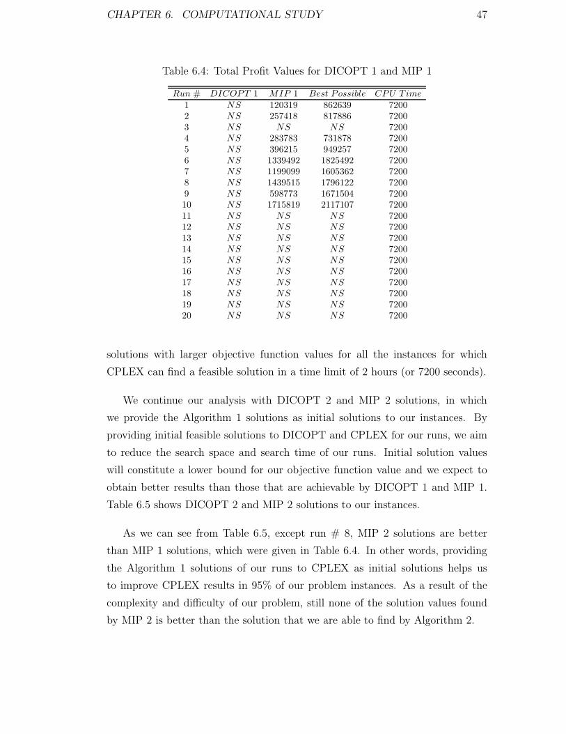
CHAPTER 6. COMPUTATIONAL STUDY 47
Table 6.4: Total Profit Values for DICOPT 1 and MIP 1
Run # DICOPT 1 MIP 1 Best Possible CPU T ime
1 NS 120319 862639 72002 NS 257418 817886 72003 NS NS NS 72004 NS 283783 731878 72005 NS 396215 949257 72006 NS 1339492 1825492 72007 NS 1199099 1605362 72008 NS 1439515 1796122 72009 NS 598773 1671504 720010 NS 1715819 2117107 720011 NS NS NS 720012 NS NS NS 720013 NS NS NS 720014 NS NS NS 720015 NS NS NS 720016 NS NS NS 720017 NS NS NS 720018 NS NS NS 720019 NS NS NS 720020 NS NS NS 7200
solutions with larger objective function values for all the instances for which
CPLEX can find a feasible solution in a time limit of 2 hours (or 7200 seconds).
We continue our analysis with DICOPT 2 and MIP 2 solutions, in which
we provide the Algorithm 1 solutions as initial solutions to our instances. By
providing initial feasible solutions to DICOPT and CPLEX for our runs, we aim
to reduce the search space and search time of our runs. Initial solution values
will constitute a lower bound for our objective function value and we expect to
obtain better results than those that are achievable by DICOPT 1 and MIP 1.
Table 6.5 shows DICOPT 2 and MIP 2 solutions to our instances.
As we can see from Table 6.5, except run # 8, MIP 2 solutions are better
than MIP 1 solutions, which were given in Table 6.4. In other words, providing
the Algorithm 1 solutions of our runs to CPLEX as initial solutions helps us
to improve CPLEX results in 95% of our problem instances. As a result of the
complexity and difficulty of our problem, still none of the solution values found
by MIP 2 is better than the solution that we are able to find by Algorithm 2.

CHAPTER 6. COMPUTATIONAL STUDY 48
Table 6.5: Total Profit Values for DICOPT 2 and MIP 2
Run # DICOPT 2 MIP 2 Best Possible CPU T ime
1 NS 478044 792832 72002 NS 536910 760823 72003 NS 699150 943616 72004 NS 354909 687143 72005 NS 583862 951209 72006 NS 1465125 1754679 72007 NS 1312737 1568786 72008 NS 1401586 1718384 72009 NS 1321299 1615406 720010 NS 1882792 2117928 720011 NS 668407 957151 720012 NS 478329 809448 720013 NS 401048 846789 720014 NS 586373 894127 720015 NS 657755 954369 720016 NS 1516720 1783367 720017 NS 1663509 1999991 720018 NS 1200298 1598373 720019 NS 1042092 1460130 720020 NS 1205923 1549724 7200
Another important improvement that we achieve by providing initial solutions
is that we can significantly reduce the gap between the best possible values and
the solutions that CPLEX find in 2 hours. One of the main reasons for these
improvements is that except one instance, Algorithm 1 solutions are better than
MIP 1 solutions in terms of objective function values. Another reason is that
providing an initial solution help to reduce the search space for our instances.
Table 6.6 shows MIP 1 and MIP 2 gaps, which are the differences between the
best possible values and the Total Profit values of the best integer solutions found
for the corresponding runs. The percentage of decrease in gaps is calculated by
the following formula:
GMIP1−MIP2 =(MIP 1 gap)− (MIP 2 gap)
(MIP 1 gap)∗ 100
Providing initial solutions to CPLEX helps to obtain an average of 42.2%
decrease in the gaps. Such decreases in the gaps between the best possible values
and the solutions found help us to ensure that we get closer to the optimal values
by providing initial solutions to CPLEX.

CHAPTER 6. COMPUTATIONAL STUDY 49
Table 6.6: Gap values for MIP 1 and MIP 2
Run # MIP 1 gap MIP 2 gap GMIP1−MIP2
1 742320 314788 57.62 560468 223913 60.13 − 244466 −4 448095 332234 25.95 553042 367347 33.66 486000 289554 40.47 406263 256049 37.08 356607 316798 11.29 1072731 294107 72.610 401288 235136 41.411 − 288744 −12 − 331119 −13 − 445741 −14 − 307754 −15 − 296614 −16 − 266647 −17 − 336482 −18 − 398075 −19 − 418038 −20 − 343801 −
Up until now, we were able to show that in all of the instances, we can find
better solutions with Algorithm 2 than the ones that can be found by CPLEX
with or without initial solutions. While finding better solutions is still meaningful,
there is also another point that we should take into consideration. This another
important point is the time that we spent to solve our instances. In Table 6.7,
we give a comparison of the objective function values and solution times that we
spent to solve our instances between Algorithm 2 and CPLEX. Although very
few, there may be instances in which MIP 1 can find a solution that is better than
the one that can be found by MIP 2 in terms of Total Profit value. Therefore,
while comparing Algorithm 2 and CPLEX, we take the best of MIP 1 and MIP
2 solutions for the corresponding runs. The percentage of the difference in Total
Profit Values between CPLEX and Algorithm 2 solutions is calculated by the
following formula:
DCPLEX−Alg2 =(Algorithm 2 value)− (Best of MIP 1 and MIP 2 value)
(Best of MIP 1 and MIP 2 value)∗ 100
As we mentioned before, we run DICOPT and CPLEX for 2 hours for each

CHAPTER 6. COMPUTATIONAL STUDY 50
Table 6.7: Total Profit Values and CPU Times for CPLEX and Algorithm 2
Best of MIP Alg 2Run # MIP 1 and MIP 2 CPU T ime Alg 2 CPU T ime DCPLEX−Alg2
1 478044 7200 507430 3.5 6.22 536910 7200 557526 2.7 3.83 699150 7200 699150 5.6 0.04 354909 7200 399544 3.0 12.65 583862 7200 622650 3.8 6.66 1465125 7200 1493919 2.8 2.07 1312737 7200 1339032 2.7 2.08 1439515 7200 1509570 2.3 4.99 1321299 7200 1321299 4.0 0.010 1882792 7200 1882792 2.2 0.011 668407 7200 713824 8.4 6.812 478329 7200 583417 13.4 22.013 401048 7200 453502 263.6 13.114 586373 7200 634184 7.1 8.215 657755 7200 723984 14.6 10.116 1516720 7200 1558088 4.2 2.717 1663509 7200 1725291 8.4 3.718 1200298 7200 1272524 32.9 6.019 1042092 7200 1130496 363.3 8.520 1205923 7200 1210876 214.6 0.4
of the DICOPT 1, MIP 1, DICOPT 2 and MIP 2 versions of our 20 runs. By
Algorithm 2, we are able to find solutions that are on the average 6.0% better
than the corresponding best of MIP 1 and MIP 2 solutions in terms of the Total
Profit value. In addition to finding better solutions to our instances, Table 6.7
shows that Algorithm 2 performs much better in terms of CPU times with respect
to DICOPT or CPLEX. A relatively large number of stations required to obtain
a solution y found by Algorithm 1 increases the search space and search time of
our surrogate problem, resulting in relatively greater CPU times in some of the
runs (i.e., runs 13, 19 and 20).
In order to find the optimal Total Profit values, we abolished the CPU time
restriction and ran CPLEX on a computer with 8 GB memory, Xeon 2.66 GHZ
CPU and Linux operating system for the first MIP 2 runs of the first two clusters,
in which the number of models is equal to 2 and the problems are relatively easier
to be solved by CPLEX. However, after 72660 seconds (20 hours and 11 minutes)

CHAPTER 6. COMPUTATIONAL STUDY 51
and 45840 seconds (12 hours and 44 minutes) for the runs 1 and 6 respectively,
CPLEX terminated due to ’out of memory’ error since the tree sizes grew to 4.5
GB. The best integer solution found for run 1 was 507430, which is also the Total
Profit value that we found by Algorithm 2. The upper bound for the Total Profit
value for run 1 was 536671, which implies a 5.7% of gap between the best solution
found and the best possible solution in terms of the Total Profit value. The best
solution found for run 6 had a Total Profit value of 1509221, which is only 1%
better than the Total Profit value that we found by Algorithm 2. The upper
bound for the Total Profit value for run 6 was 1546606, which implies a 2.5%
of gap between the best solution found and the best possible solution in terms
of the Total Profit value. Looking at these results and Example 3 provided in
section 4.2, we can say that Algorithm 2 is capable of finding very good solutions
to instances of our problem. Also, it would probably take several days to solve
the MIP versions of our runs to optimality by CPLEX.
As we mentioned before, the values of the two factors, the number of differ-
ent models to be produced in the assembly line and the the ratio PRh
Vjplay an
important role for the Total Profit values of our solutions and the Heuristic, DI-
COPT and CPLEX performances. Table 6.8 is a summary of the cluster based
evaluation of Algorithm 1, Algorithm 2 and CPLEX.
Table 6.8: Solution Analysis for Problem Clusters
Factor IAlg1−Alg2 DAlg1−CPLEX DCPLEX−Alg2
h PRVj
Min Ave Max Min Ave Max Min Ave Max
L L 0.0 10.1 21.2 0.0 4.1 16.7 0.0 5.8 12.6L H 0.0 4.9 11.7 0.0 2.9 6.5 0.0 1.8 4.9H L 6.8 12.0 22.0 0.0 0.0 0.0 6.8 12.0 22.0H H 0.4 4.3 8.5 0.0 0.0 0.0 0.4 4.3 8.5
When the number of models is at its low level, Algorithm 1 sometimes works
as well as Algorithm 2. However, in all of the runs with the number of models at
the high level, we obtain better results with Algorithm 2 because as the number of
models increase, the total number of operations increase and hence the probability
of improving Algorithm 1 allocations by the surrogate problem and obtaining
better solutions increase. The improvements are more significant especially in the

CHAPTER 6. COMPUTATIONAL STUDY 52
runs with low PRh
Vjratios because the Total Profit values are relatively smaller
when PRh
Vjratios are at the low level and as a result, improvements on Algorithm
1 solutions in terms of Total Profit values correspond to higher percentages. In
addition to this, CPLEX can improve the initial solutions found by Algorithm 1
in 5 of the 10 runs with low number of models and fails to improve any of the
solutions found by Algorithm 1 for the runs with high number of models. Again,
CPLEX improvements on Algorithm 1 solutions are more significant when the
ratio PRh
Vjis at its low level. Moreover, except for 3 runs, Algorithm 2 finds better
solutions than CPLEX in terms of the Total profit values and the differences
between Algorithm 2 and CPLEX solutions are more significant in the runs with
low PRh
Vjratios. The reason of why Algorithm 2 can not find a better solution
than CPLEX solutions in 3 of the runs is that in these 3 runs, Algorithm 1 and
Algorithm 2 Total Profit values are the same and that CPLEX takes Algorithm
1 solutions as initial feasible solutions.
In summary, in this chapter of our study, we tested the performance of our
heuristic algorithm on some instances of our problem that are created randomly.
The results of the comparison between our heuristic and GAMS solvers DICOPT
and CPLEX showed that our heuristic is very efficient in terms of the CPU time
and the quality of the solutions found. The next chapter of this thesis is devoted
to concluding remarks.

Chapter 7
Conclusion
In this study, we considered a mixed-model assembly line design problem with
the objective of maximizing the total profit that would be gained from the as-
sembly line. In the assembly line, different models are produced in an intermixed
sequence. Due to the similarities between the production processes of different
models, setup times are not present. Instead of assuming continuous production,
we dealt with designing an assembly line that works 24 hours a day in three 8-
hour shifts. We considered a 10-minute break between the shifts and a 30-minute
lunch break and two 10-minute tea breaks in each shift. Considering limited tool
lives for the tools used for production in the assembly line gives rise to the neces-
sity of determining the replacement times of the tools. In many industries, tool
change related assembly line stoppages result in loss of production and so are
very costly. In our study, we eliminate such a problem by restricting tool changes
to be performed only in the aforementioned breaks.
We first formulated our assembly line design problem as a Nonlinear Mixed
Integer Programming (NLMIP) model and tried to solve our problem with DI-
COPT. Due to the size and difficulty of our problem, DICOPT failed to find a
feasible solution to any one of the generated instances, which we think closely
represent real life problems that we have observed during our collaboration with
the automotive industry. Therefore, we linearized our problem and tried to solve
53

CHAPTER 7. CONCLUSION 54
the Mixed Integer Programming (MIP) version of our problem by CPLEX. How-
ever, CPLEX also failed to solve our problem in the preset time limit and could
not find even a feasible solution for several instances.
Upon not obtaining optimal solutions from DICOPT and CPLEX (we may
not even have a feasible solution for larger problem instances), we developed
a heuristic algorithm to obtain a set of feasible solutions. Finding alternative
solutions rather than a single solution allows us to perform a search for the
best solution. In addition to this, we improved our heuristic by incorporating
a surrogate problem and obtained a stronger heuristic, which performed better
in terms of objective function values of the solutions found. We compared the
results of the heuristic algorithms given in Sections 4.1 (Algorithm 1) and 4.2
(Algorithm 2) with commercial solvers DICOPT and CPLEX. We also provided
the best Algorithm 1 solutions as initial solutions to DICOPT and CPLEX in
order to increase their performances. By doing so, we observed that CPLEX
could find better solutions in terms of the objective function value and the gap
between the objective function values of the best integer solution found and the
best possible solution decreased. However, Algorithm 2 outperformed DICOPT
and CPLEX in many instances and proved to be very efficient in terms of the
solution times and the objective function values of the solutions found.
The existing studies in the literature overlook the limited lives of the tools
that are used for production and hence ignore tool change decisions. However,
in most of the industries, the tools that are used for production have limited
tool lives. As we saw in Chapter 5, assembly lines may suffer from tool change
related stoppages unless the tool lives are taken into consideration while allocating
operations to the stations in the assembly line. Moreover, real-life assembly line
problem formulations may take a very long time to be solved by commercial
solvers. Hence, by representing a more realistic production environment and
with the efficient solution techniques provided, we hope that our study will be a
remarkable contribution to the existing literature.
Our study is the first one to consider tool changes in the assembly lines and
to eliminate the tool change related line stoppages. For future research, this

CHAPTER 7. CONCLUSION 55
study can be extended to the cases in which there may be multiple robots in the
stations of the assembly line. Our problem is more applicable on the existing
assembly lines, which are subject to model changes. But, if an assembly line is to
be set up for the first time, tool selection decision can be added to our problem
by incorporating tool selection decision variables. Furthermore, as Gultekin et
al. [11] did, flexibility can be added to the scope of our study by considering
controllable processing times instead of using deterministic processing times for
the assembly line operations. In addition to these, by adding assembly line setup
times for the models to be produced, our problem can be converted to a multi-
model assembly line problem, in which an additional sequencing problem will
arise.

Bibliography
[1] R. G. Askin and M. Zhou. A parallel station heuristic for the mixed-model
production line balancing problem. International Journal of Production Re-
search, 35:3095–3105, 1997.
[2] I. Baybars. An efficient heuristic method for the simple assembly line bal-
ancing problem. International Journal of Production Research, 24:149–166,
1986.
[3] I. Baybars. A survey of exact algorithms for the simple assembly line bal-
ancing problem. Management Science, 32:909–932, 1986.
[4] C. Becker and A. Scholl. A survey on problems and methods in generalized
assembly line balancing. European Journal of Operational Research, 168:694–
715, 2006.
[5] J. Bukchin, E. M. Dar-el, and J. Rubinovitz. Mixed-model assembly line de-
sign in a make-to-order environment. Computers and Industrial Engineering,
41:405–421, 2002.
[6] Y. Bukchin and I. Rabinowitch. A branch-and-bound based solution ap-
proach for the mixed-model assembly line-balancing problem for minimizing
stations and task duplication costs. European Journal of Operational Re-
search, 174:492–508, 2005.
[7] E. Erel and H. Gokcen. Shortest route formulation of mixed-model assembly
line balancing problem. European Journal of Operational Research, 116:194–
204, 1999.
56

BIBLIOGRAPHY 57
[8] E. Erel, I. Sabuncuoglu, and B. A. Aksu. Balancing of U-type assembly
line systems using simulated annealing. International Journal of Production
Research, 39:3003–3015, 2001.
[9] E. Erel, I. Sabuncuoglu, and H. Sekerci. Stochastic assembly line balancing
using beam search. International Journal of Production Research, 43:1411–
1426, 2005.
[10] K. Fleszar and K. S. Hindi. An enumerative heuristic and reduction methods
for the assembly line balancing problem. European Journal of Operational
Research, 145:606–620, 2003.
[11] H. Gultekin, M. S. Akturk, and O. Karasan. Bicriteria robotic cell schedul-
ing. Journal of Scheduling, 11:457–473, 2008.
[12] A. N. Haq, J. Jayaprakash, and K. Rengarajan. A hybrid genetic algorithm
approach to mixed-model assembly line balancing. International Journal of
Advanced Manufacturing Technology, 28:337–341, 2006.
[13] N. V. Hop. A heuristic solution for fuzzy mixed-model line balancing prob-
lem. European Journal of Operational Research, 168:789–810, 2006.
[14] G. Levitin, J. Rubinovitz, and B. Shnits. A genetic algorithm for robotic
assembly line balancing. European Journal of Operations Research, 168:811–
825, 2006.
[15] S. Matanachai and C. A. Yano. Balancing mixed-model assembly lines to
reduce work overload. IIE Transactions, 33:29–42, 2001.
[16] P. R. McMullen and P. Tarasewich. Using ant techniques to solve the as-
sembly line balancing problem. IIE Transactions, 35:605–617, 2003.
[17] C. Merengo, F. Nava, and A. Pozetti. Balancing and sequencing manual
mixed-model assembly lines. International Journal of Production Research,
37:2835–2860, 1999.
[18] J. Miltenburg. Balancing and scheduling mixed-model U-shaped production
lines. International Journal of Flexible Manufacturing Systems, 14:119–151,
2002.

BIBLIOGRAPHY 58
[19] B. Rekiek, P. de Lit, F. Pellichero, T. L’Eglise, P. Fouda, E. Falkenauer,
and A. Delchambre. A multiple objective grouping genetic algorithm for
assembly line balancing. Journal of Intelligent Manufacturing, 12:467–485,
2001.
[20] T. Sawik. Monolithic vs. hierarchical balancing and scheduling of a flexible
assembly line. European Journal of Operational Research, 143:115–124, 2002.
[21] A. Scholl and C. Becker. State-of-the-art exact and heuristic solution pro-
cedures for simple assembly line balancing. European Journal of Operations
Research, 168:666–693, 2006.
[22] A. Scholl and R. Klein. Balancing assembly lines effectively–a computational
comparison. European Journal of Operational Research, 114:50–58, 1999.
[23] D. Sparling and J. Miltenburg. The mixed-model U-line balancing problem.
International Journal of Production Research, 36:485–501, 1998.
[24] P. M. Vilarinho and A. S. Simaria. An ant colony optimization algorithm
for balancing mixed-model assembly lines with parallel workstations. Inter-
national Journal of Production Research, 44:291–303, 2006.
[25] W. E. Wilhelm and R. Gadidov. A branch-and-cut approach for a generic
multiple-product, assembly-system design problem. INFORMS Journal on
Computing, 16:39–55, 2004.

Appendix A
Nomenclature
Problem Parameters
Vj: cost of setting up station j, j ∈M .
nh: number of operations to be performed to produce model h, h ∈ G.
Whi: number of spot welds required to perform operation i of model h, i ∈ Nh,
h ∈ G.
Bj : total number of spot welds such that the welding tool in station j ∈M can
process.
Cj: cost of the welding tool in stationj, j ∈M .
θh: yearly expected demand for model h, h ∈ G.
γh: target cycle time for model h to meet the yearly expected demand θh, h ∈ G.
γLh : lower bound for the actual cycle time of model h, h ∈ G.
γUh : upper bound for the actual cycle time of model h, h ∈ G.
PRh: profit contributed by each component of model h produced, h ∈ G.
PRǫh: profit contributed by each excess component of model h produced, h ∈ G.
ahij = 1, if operation i ∈ Nh of model h ∈ G can be assigned to station j ∈M ;
and 0, otherwise.
phik = 1, if operation i ∈ Nh of model h ∈ G precedes operation k ∈ Nh
of model h ∈ G; and 0, otherwise.
thi: the time required to perform operation i ∈ Nh of model h ∈ G.
Dq: available tool change time in tool change period q, q = 1, 2, . . . , U .
59
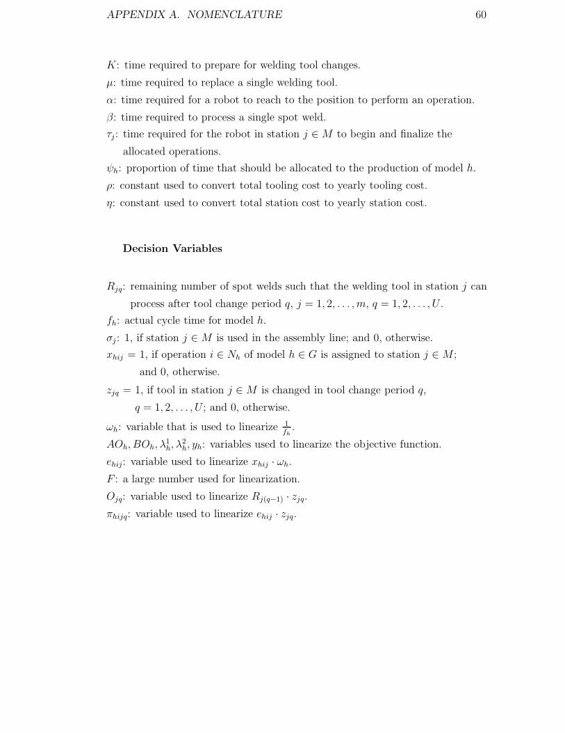
APPENDIX A. NOMENCLATURE 60
K: time required to prepare for welding tool changes.
µ: time required to replace a single welding tool.
α: time required for a robot to reach to the position to perform an operation.
β: time required to process a single spot weld.
τj : time required for the robot in station j ∈M to begin and finalize the
allocated operations.
ψh: proportion of time that should be allocated to the production of model h.
ρ: constant used to convert total tooling cost to yearly tooling cost.
η: constant used to convert total station cost to yearly station cost.
Decision Variables
Rjq: remaining number of spot welds such that the welding tool in station j can
process after tool change period q, j = 1, 2, . . . , m, q = 1, 2, . . . , U .
fh: actual cycle time for model h.
σj : 1, if station j ∈M is used in the assembly line; and 0, otherwise.
xhij = 1, if operation i ∈ Nh of model h ∈ G is assigned to station j ∈M ;
and 0, otherwise.
zjq = 1, if tool in station j ∈M is changed in tool change period q,
q = 1, 2, . . . , U ; and 0, otherwise.
ωh: variable that is used to linearize 1fh
.
AOh, BOh, λ1h, λ
2h, yh: variables used to linearize the objective function.
ehij: variable used to linearize xhij · ωh.
F : a large number used for linearization.
Ojq: variable used to linearize Rj(q−1) · zjq.
πhijq: variable used to linearize ehij · zjq.

VITA
Adnan Tula was born on March 3, 1985 in Isparta, Turkiye. He received his high
school education at Antalya Ozel Mahmut Celal Unal Fen Lisesi, Turkiye. He has
received his B.S. degree from the Department of Industrial Engineering, Bilkent
University in 2007. Since September 2007, he has been working with Prof. Selim
Akturk for his graduate study at the same department.
61