robotic tooling calibration based on...
TRANSCRIPT

Toronto, Ontario, Canada, 2015
© Mohamed Helal, 2015
ROBOTIC TOOLING CALIBRATION BASED ON LINEAR AND
NONLINEAR FORMULATIONS
By
Mohamed Helal, B.Eng
Aerospace Engineering
Ryerson University, 2013
A thesis presented to Ryerson University
in partial fulfillment of the requirement for the degree of
Master of Applied Science
in the Program of
Aerospace Engineering

ii
AUTHOR’S DECLARATION
I hereby declare that I am the sole author of this thesis. This is a true copy of the thesis,
including any required final revisions, as accepted by my examiners.
I authorize Ryerson University to lend this thesis to other institutions or individuals for
the purpose of scholarly research.
I further authorize Ryerson University to reproduce this thesis by photocopying or by
other means, in total or in part, at the request of other institutions or individuals for the purpose
of scholarly research. I understand that my thesis may be made electronically available to the
public.

iii
ABSTRACT
Robotic Tooling Calibration Based on Linear and Nonlinear Formulations
Mohamed Helal
A thesis of the degree of
Masters of Applied Science, 2015
Department of Aerospace Engineering, Ryerson University
Industrial robot calibration packages, such as ABB CalibWare, are developed only for
robot calibration. As a result, the robotic tooling systems designed and fabricated by the user are
often calibrated in an ad-hoc fashion. In this thesis, a systematic way for robotic tooling
calibration is presented in order to overcome this problem. The idea is to include the tooling
system as an extended body in the robot kinematic model, from which two error models are
established. The first error model is associated with the robot, while the second error model is
associated with the tooling. Once the robot is fully calibrated, the first error will be reduced to
the required accuracy. Thus, the method is focused on the second error model. For the tool error
calibration, two formulations were used. The first is a linear formulation based on conventional
calibration as well as self-calibration methods while the second is a nonlinear formulation. The
conventional linear formulation was extensively investigated and implemented while the self-
calibration was proven to be inadequate for the tooling calibration. Moreover, the nonlinear
formulation was demonstrated to be very effective and accurate through experimental result. The
end-effector position estimation as well as the tool pose estimation were obtained using a 3D
vision system as an off-line error measurement technique.

iv
ACKNOWLEDGEMENTS
I would like to express my deepest appreciation to my supervisor Dr. Jeff Xi, for his
extensive guidance, support and encouragement not only during my master’s degree but also
during my undergraduate degree. His great knowledge and patience have been really helpful for
guiding me towards the right path to solve all the problems I faced. It has been a great pleasure
for me to work under his supervision.
I would also like to offer my specials thanks to Mr. Yu Lin for all his help, time and
effort during my research period.
In addition, I would like to express my gratitude to all my co-workers at Amel Group
especially Ms. Johanna Malisani, Mr. Peter Cresnik and Mr. Khalid Saleh for their help and
support.
Last but not least, I would like to thank my family and friends for their support,
encouragement and understanding during the past school years.
v
TABLE OF CONTENTS
Author’s Declaration ....................................................................................................................... ii
Abstract .......................................................................................................................................... iii
Acknowledgements ........................................................................................................................ iv
Table of Contents ............................................................................................................................ v
List of Tables ............................................................................................................................... viii
List of Figures ................................................................................................................................. x
Nomenclature ............................................................................................................................... xiii
Chapter 1: Introduction ................................................................................................................... 1
1.1 Background and Objectives ............................................................................................... 2
1.2 Thesis Organization ........................................................................................................... 8
Chapter 2: Literature Review ........................................................................................................ 10
2.1 Kinematic Modeling for Manipulator Calibration ........................................................... 11
2.2 Measurement Tools.......................................................................................................... 14
2.2.1 Laser Tracking Systems ......................................................................................... 16
2.2.2 Laser Interferometers ............................................................................................. 16
2.2.3 Coordinate Measuring Machines (CMMs) ............................................................ 17
2.2.4 Camera Type Devices ............................................................................................ 19
2.2.5 Theodolites ............................................................................................................ 20
2.2.6 Wire-Draw Encoders ............................................................................................. 21
2.3 Identification .................................................................................................................... 22
2.4 Implementation ................................................................................................................ 26
2.5 Self-Calibration ................................................................................................................ 27

vi
2.6 Tool Center Point (TCP) Localization ............................................................................. 28
2.7 Hand-Eye Calibration ...................................................................................................... 31
Chapter 3: Kinematic and Error Modelling .................................................................................. 34
3.1 System Description .......................................................................................................... 36
3.2 Robot Kinematic Modelling with Tool ............................................................................ 38
3.2.1 Position and Orientation ........................................................................................ 38
3.2.2 Calibration System Kinematic Modeling .............................................................. 40
3.3 Error Modelling ............................................................................................................... 43
Chapter 4: Calibration Algorithm ................................................................................................. 45
4.1 Linear Formulation .......................................................................................................... 45
4.1.1 Eye-to-Hand vs. Eye-in-Hand ............................................................................... 47
4.1.2 Geometric Errors ................................................................................................... 48
4.1.3 Jacobian Matrix ..................................................................................................... 49
4.2 Nonlinear Formulation ..................................................................................................... 53
4.2.1 Genetic Algorithm ................................................................................................. 54
4.3 Calibration Formulation ................................................................................................... 57
4.4 On-line vs. Off-line Error Measurement.......................................................................... 59
4.4.1 On-line Error Measurement for Robots ................................................................. 59
4.4.2 On-line Error Measurement for Robotic Tooling Calibration ............................... 62
4.4.3 Off-line error measurement for Non-linear Tool Calibration formulation ............ 67
Chapter 5: Measurements Simulations ......................................................................................... 68
5.1 Measurement System ....................................................................................................... 68
5.2 End-Effector Position Estimation .................................................................................... 70

vii
5.3 Tool Pose Estimation ....................................................................................................... 75
5.3.1 Fitness Function ..................................................................................................... 77
5.4 End-Effector Simulation .................................................................................................. 80
5.5 Tool Simulation ............................................................................................................... 82
Chapter 6: Experiments................................................................................................................. 87
6.1 End-Effector Pose Estimation .......................................................................................... 87
6.2 Tool Pose Estimation ....................................................................................................... 90
6.3 Linear Full Pose Calibration ............................................................................................ 96
6.4 Nonlinear Position Calibration ........................................................................................ 97
6.5 Nonlinear Orientation Calibration ................................................................................... 98
6.6 Nonlinear Full Pose Calibration .................................................................................... 101
Chapter 7: Conclusion, Contributions and Future Work ............................................................ 106
7.1 Conclusion ..................................................................................................................... 106
7.2 Contributions ................................................................................................................. 106
7.3 Future Work ................................................................................................................... 107
List of Appendices ...................................................................................................................... 109
Appendix A – Plane Fitting ................................................................................................. 109
Appendix B – Kasa Method ................................................................................................ 110
Appendix C– Cylinder Equations ........................................................................................ 111
Appendix D – Robot End-Effector in Base Frame .............................................................. 113
Appendix E – Jacobian Matrix ............................................................................................ 113
Appendix F – 3D Vision System ......................................................................................... 114
References ................................................................................................................................... 116

viii
LIST OF TABLES
Table 5-1: Circle Fitting Methods Results .................................................................................... 73
Table 5-2: Simulated Cylinder Data Points Parameters ............................................................... 79
Table 5-3: Estimated GA Cylinder Parameters ............................................................................ 80
Table 6-1: End-Effector Location with Respect to the Camera Frame ........................................ 88
Table 6-2: Cylinder GA Results with respect to the Intermediate Frame ..................................... 92
Table 6-3: Monte Carlo Simulation Results ................................................................................. 94
Table 6-4: Measured and Nominal Rotation Matrices and Position Vectors ............................... 95
Table 6-5: Linear Formulation Estimated Geometric Errors ........................................................ 97
Table 6-6: Calibrated Tool Pose Rotation Matrix and Position Vector ........................................ 97
Table 6-7: Position Errors ............................................................................................................. 97
Table 6-8: Calibrated Position ...................................................................................................... 98
Table 6-9: Orientation Errors for 500 Generations and 100 Population Size ............................... 99
Table 6-10: Measured, Nominal and Calibrated Rotation Matrices with respect to the Camera
frame ........................................................................................................................................... 100
Table 6-11: Errors with 500 Generations and 300 Population Size............................................ 101
Table 6-12: Position and Orientation Errors Based on 500 Generations and 100 Population Size
..................................................................................................................................................... 102
Table 6-13: Calibrated Rotation Matrix and Position Vector Based on 500 Generations and 100
Population size ............................................................................................................................ 103
Table 6-14: Position and Orientation Errors with 500 Generations and 300 Population Size ... 103
Table 6-15: Calibrated Rotation Matrix and Position Vector Based on 500 Generations and 300
Population Size ........................................................................................................................... 104
Table 6-16: Position and Orientation Errors with 500 Generations and 500 Population Size ... 104

ix
Table 6-17: Calibrated Rotation Matrix and Position Vector Based on 500 Generations and 500
Population Size ........................................................................................................................... 105
Table A-1: End-Effector Parameters with respect to the Base Frame ........................................ 113
Table A-2: Rotation Matrix and Position Vector of the End-Effector with respect to the Base
Frame .......................................................................................................................................... 113

x
LIST OF FIGURES
Figure 2-1: Laser Tracking Concept Diagram [5]. ....................................................................... 16
Figure 2-2: Laser Interferometer Concept Diagram [16] .............................................................. 17
Figure 2-3: Modern CMM Machine [32] ...................................................................................... 18
Figure 3-1: Automated Percussive Riveting System .................................................................... 36
Figure 3-2: Robotic System with Frames ..................................................................................... 37
Figure 3-3: Robot Tool System..................................................................................................... 38
Figure 3-4: Position Vector ........................................................................................................... 38
Figure 3-5: Robot - 3D Vision System Diagram .......................................................................... 41
Figure 4-1: Tool - End-Effector Relation ..................................................................................... 48
Figure 4-2: Genetic Algorithm...................................................................................................... 54
Figure 4-3: Calibration Algorithm ................................................................................................ 58
Figure 4-4: Robot Tool-Camera System CAD Model .................................................................. 63
Figure 4-5: Superimposed Theoretical Robotic Links .................................................................. 63
Figure 4-6: Final Theoretical model diagram. .............................................................................. 64
Figure 5-1: Camera Unit ............................................................................................................... 69
Figure 5-2: Hand-Held Digitizer Gun ........................................................................................... 69
Figure 5-3: Robot's End-Effector .................................................................................................. 70
Figure 5-4: Circle Fitting using Kasa Method vs. Least Square Method ..................................... 73
Figure 5-5: 3D Space Circle Fitting Algorithm ............................................................................ 74
Figure 5-6: Simulated 3D Circle Fitting Algorithm ..................................................................... 75
Figure 5-7: Pneumatic Rivet Gun ................................................................................................. 76
Figure 5-8: Cylinder in General Orientation ................................................................................. 78

xi
Figure 5-9: Generated Point Cloud and Best Fit Cylinder ............................................................ 79
Figure 5-10: Cylinder Fitting GA with 500 Generations and 500 Population Size ...................... 80
Figure 5-11: Circle Simualtion Data Points .................................................................................. 81
Figure 5-12: Circle Center Accuracy vs. Number of Points ......................................................... 82
Figure 5-13: Cylinder Point Cloud with Noise ............................................................................. 83
Figure 5-14: Normal Distribution and Uniform Distribution ....................................................... 84
Figure 5-15: RMSPE vs. Number of Points.................................................................................. 85
Figure 5-16: RMSOE vs. Number of Points ................................................................................. 85
Figure 5-17: Radius Error vs. Number of Points .......................................................................... 86
Figure 6-1: Experimental Circle Data Points (mm) ...................................................................... 88
Figure 6-2: End-Effector Center and Frame Determination ......................................................... 89
Figure 6-3: Experimental Cylinder Data Points (mm) .................................................................. 90
Figure 6-4: Introducing an Intermediate Frame Diagram ............................................................. 91
Figure 6-5: Cylinder Fitting GA with 500 Generations and 500 Population Size. ....................... 93
Figure 6-6: Cylinder Fitting Experimental Point Cloud ............................................................... 94
Figure 6-7: Camera, End-Effector and Gun Set-up Diagram ....................................................... 95
Figure 6-8: Linear Calibration RMSE vs. Number of Iterations .................................................. 96
Figure 6-9: Position Only Calibration with 500 Generations and 100 Population Size ............... 98
Figure 6-10: Orientation Only Calibration with 500 Generations and 100 Population Size ........ 99
Figure 6-11: Orientation Only Calibration with 500 Generations and 300 Population Size ...... 101
Figure 6-12: Full Pose Calibration with 500 Generations and 100 Population Size .................. 102
Figure 6-13: Full Pose Calibration with 500 Generations and 300 Population Size .................. 103
Figure 6-14: Full Pose Calibration with 500 Generations and 500 Population Size .................. 104

xii
Figure A-1: Best Fit Plane Generated for Multiple Points ......................................................... 109
Figure A-2: Cylinder Rotation Sequence .................................................................................... 112

xiii
NOMENCLATURE
Symbols Definition
Center Location Corresponding to X and Y Axes
Radius
Weighting Factors
Augmented Diagonal Matrix of Rotation Matrices
Self-Calibration Measurements Matrix
Robot Geometric Parameters
Nominal Geometric Parameters
Nominal Robot Geometric Parameters
Nominal Tool Geometric Parameters
Calibrated Robot Geometric Parameters
Self-Calibration Jacobian Matrix
Tool Jacobian Matrix in the Base Frame
Jacobian Pseudo Inverse
Jacobian Matrix for Camera Frame
Position Vector
Tool Length Position Vector
Normalized Tool Length Position Vector
Joint Variables
Nominal Joint Variables
Rotation Matrix
Homogeneous Transformation
Robot Tip Pose
Measured Target Position
Actual Target Position
Measured Tool Tip Pose
Nominal Tool Tip Pose
Augmented Tip Errors Vector
Augmented Tip Errors Vector for Self-Calibration
Robot Tip Pose Errors
Robot Geometric Parameters errors

xiv
Robot Joint Variables Compensation
Compensation Errors
Block Diagonal Matrix of Rotation Matrices
Orientation Angles Vector
Sub/Superscripts Definition
C Camera Frame
m Measured
o Nominal
R Robot Frame
r Robot
T Tool Frame
t Tool
Tip Tool Tip Frame
V 3D Vision System Frame

1
CHAPTER 1: INTRODUCTION
Presented in this thesis is a development of a novel method for robotic manipulator tool
center point calibration. This chapter is composed of two main sections that provide a full and
quick overview of the topics discussed in the following thesis.
The first section of this chapter provides a general overview of the thesis background
regarding multiple topics. It starts by a brief history of the industrial automation development
during the last few decades. It also provides a complete description of the robotic manipulators
and their characteristics as well as their advantages and disadvantages. It progresses by
discussing the main disadvantages focusing on the lack of accuracy of its main sources and
potential solutions available. Subsequently, an introduction to the calibration process steps is
discussed. Calibration process is also introduced from a mathematical point of view as an
optimization problem and its possible solutions. The user problem regarding tool center point
determination is also explained. Finally, this section ends by listing all the assumptions taken
into consideration as well as the objectives and contributions of the thesis.
The second section of this chapter includes a full outline of the thesis and a brief
explanation of each of the following chapters.

2
1.1 Background and Objectives
Major industries such as aerospace and automotive industries are mainly focusing on
increasing their productivity rates by increasing the efficiency of their industrial processes. As a
result, the main trend is directed towards the automation of most of these processes. Since the
use of the first automated robotic system in the early 1960s and until the current date, industrial
automation using robotic systems has been rapidly developed and perfected to perform several
production tasks [1]. Spray painting, welding, assembly and material handling are some
examples of the tasks that could be performed by industrial robots today.
The development of industrial robotic systems is a result of the progress in several
disciplines such as mechanical, electrical, programming and control sciences. An industrial robot
is a mechanically actuated mechanism that is controlled by a means of a computer system.
Unfortunately, an exact definition of an industrial robot is not clearly provided as it is
occasionally disputed amongst specialists [2]. In general, an industrial robot is a multipurpose
mechanical system that can be programmed to execute various tasks. They are also characterized
by operating in wide workspace compared to the volume they occupy. For example a computer
numerical controlled (CNC) machine is not considered to be an industrial robot because it is
specifically built for performing particular tasks. Their volumetric space is also much larger than
their workspace field [1].
Industrial robotic manipulator is a mechanical structure that resembles the human arm. It
consists of a series of links connected together with joints. It is fixed at the base on one end and
at the other side it ends with an end-effector or tool. The movement of the robotic manipulator is
being actuated at each axis of motion such as rotational and/or translational axis. The position

3
and the velocity of each of the robot’s joints are being determined by a means of internal sensors
and encoders. The information determined by the sensors and encoders are fed back to the
robot’s controller which in turn calculates the predicted position and orientation of the end-
effector. The controller then commands the actuators to implement the identified program under
the guidance of a human control to drive the end-effector to reach the intended position and
orientation. Due to several sources of inaccuracies, there is always a discrepancy between the
actual end-effector’s pose and the intended pose.
There are two main terms that are considered to be an attribute of the performance of
robotic manipulators; accuracy and repeatability. The understanding of these two terms is mainly
dependent on the understanding of the different error types. Errors can be divided into two main
types; random errors and systematic errors. Random errors are due to unpredictable sources and
they tend to vary the measurements uniformly around a true value. While the systematic errors
sometimes called biases is the deviation of the mean value away from the true value. The
repeatability of a robotic manipulator is the measurement of the precision or randomness of
achieving the same pose of the robot’s end-effector multiples of times under the exact same
conditions. The accuracy of the robot’s end-effector is the measurement of the closeness of the
actual pose to the required pose, which is a direct representation of the system systematic errors
[3]. In general, industrial robotic manipulators are characterized by their high repeatability which
usually varies between the values of 0.1 to 0.03 mm. On the other hand, the accuracy values of
industrial manipulators are considered to be significantly worse than their repeatability values
which usually lie in the order of 1 mm [4].

4
Robotic manipulator’s accuracy is an important factor in various industry applications.
Welding, drilling and machining are some applications that require high accuracy systems to be
performed. The position/pose of the end-effector with respect to the base of the robot or to an
external frame of reference has to be accurate enough for performing these jobs. The
inaccuracies encountered in any robotic manipulator could be divided into two main sources,
geometric and non-geometric. First, geometric errors are a result of the robotic geometric
parameters. Second, the non-geometric sources could be mapped to different factors such as
gears backlash, encoders’ accuracy, links flexibility and errors due to thermal and wear effects
[5].
Any robotic manipulator could be mathematically represented as a non-linear function of
the robot geometric parameters and joint variables. The robot geometric parameters are the
parameters that represent the geometry of the links and their connection together. However, the
joint variables are the representation of the joints displacements, for example, a revolute joint
would be presented by an angle and a prismatic joint would be presented by a length. Hence,
there are two main approaches investigated by researchers and used by industry to significantly
increase the accuracy of robotic manipulators. The first approach is called calibration which is
mainly concerned by adjusting the geometric parameters of the non-linear function to eliminate
the end-effector errors. The second approach is called compensation which focuses on correcting
the tip errors by changing the joint variables of the robot, in other words, controlling the
displacements of joints of the robotic arm.
As a result of the inherent convenience of the calibration approach with respect to the
compensation techniques, calibration became the main focus of researchers for further

5
development during the last few decades. Many techniques and algorithms have been developed
to improve the accuracy of robotic manipulators. Furthermore, many software packages were
created by robotic manufacturers such as ABB CalibWare which provide an easy and quick tool
for calibration.
Calibration process is divided into four main steps which are kinematic modeling,
measurement, identification and finally implementation. Kinematic modeling is the very first
step that is required for the calibration process. Kinematic modeling is basically formulating a
mathematical model that represents the robotic manipulator as a function of its geometric
parameters and joint variables. The second step is the measurement system which provides
sufficient information of the robot’s hand position and orientation corresponding to multiple
configurations of the manipulator. The third step is called the identification step which is mainly
concerned with using the kinematic model and the measurement information to estimate the
parameters that reduces the tip errors. Finally, implementation or correction is the step that
investigates the usage of the estimated robot’s parameters to physically increase the robot’s
accuracy [5, 16].
The main objective of any calibration problem is finding the geometric parameters that
drive the residual errors towards zero. Calibration is an iterative process that starts with an initial
guess which is close to the actual value, where the initial guess is the robot’s nominal geometric
parameters based on the robot’s CAD models. In an essence, any calibration process is
considered to be multivariable nonlinear optimization problem [16]. There are many ways for
solving an optimization problem depending on the nature of the problem. The solutions could be
divided into two main categories, namely linear and non-linear. The first approach is done by

6
approximating the whole system with a linear model and then solving it. The second approach
deals with the system as a non-linear problem using multiple ways for finding good estimates. As
a result of the advancements in computer and computational fields, search methods became a
popular non-linear approach for many researchers. One of the main advantages of the linear
approach is having a fast convergence rate towards parameters estimates. On the other hand,
linear approach exhibits many difficulties in certain conditions such as matrix singularities. This
could be avoided using non-linear approaches which are characterized by a relatively slow
convergence rate.
Robots manufacturers usually provide their customers with software programs or services
as an easy to use calibration packages. Since robotic arms have several applications, users
customize the robot for serving their needs by designing different tools and gadgets which are
mounted on the robot’s end-effector. Due to manufacturing and assembly errors encountered in
attaching an extra tool link to the robot, the overall accuracy of the robot reduces significantly.
This forces users to perform a secondary calibration process to correct the errors of the tool link.
The calibration of the tool link is done in an ad-hoc fashion, in other words, case by case
scenario. It is also usually done for specific axes, which are most relevant to the application and
not for the full pose. This is a tedious, time and money consuming process which also lacks any
systematic approach and heavily depends on the skill level of the technician performing the
calibration.
The main topic presented in the following thesis is focusing on developing a new
systematic calibration method for correcting the geometric parameters errors of the robotic
mounted-tools. The method in this thesis is developed based on the following assumptions:

7
- The geometric parameters errors of the robotic manipulator have to be calibrated to a
sufficient accuracy. In accordance to that condition the robotic manipulator was
considered to be perfectly accurate with zero errors. The following assumption is
important as the transformation vector from the robot’s end-effector flange to the
robot’s base should be perfectly known.
- The intrinsic parameters of the 3D vision system as well as the camera system have to
be determined and calibrated. The vision system and camera have to be calibrated so
they could accurately capture tip errors.
The main objectives of this thesis are summarized and listed below in the following
points:
- Develop a new robotic tool center point (TCP) calibration algorithm based on linear
and nonlinear approaches. There are two linear approaches; the first approach is
based on the conventional calibration technique using least squares while the second
approach is based on the technique developed by Gong et al. [53] for calibrating a
robotic manipulator system. The non-linear approach would be based on a widely
used computer search algorithm called genetic algorithm (GA).
- Investigate both the linear and the nonlinear formulations and determine their
limitations, advantages, disadvantages and effectiveness.
- Use a 3D vision system as well as the camera system for developing multiple
techniques for the robot’s end-effector position estimation and the tool orientation
estimation.

8
- Verify the developed techniques via computer simulations and determine the
limitations and conditions for conducting experiments.
- Finally, conduct an experiment to validate the simulation results and the overall
designed calibration formulation.
1.2 Thesis Organization
This thesis is divided into six main chapters in addition to the introduction. In this section
the organization and a complete outline of the thesis is provided as well as a concise description
of the contents of each section.
Chapter 2 is a complete survey that covers all of the topics introduced in this chapter. The
chapter starts with the four main steps of the calibration process, which are modeling,
measurement, identification and implementation. In addition, a complete section was fully
dedicated to discuss the self-calibration methods and techniques. Finally, the last two sections
provide an overview of the differences between the tool center point (TCP) calibration and the
hand-eye calibration.
Chapter 3 discusses the very first step of building a calibration model which is creating a
forward kinematic model for the given system. The problem of calibration is discussed and the
basis of the kinematic model would be introduced. Then, a full system description is provided.
Finally, an error model is created to describe the relation between the tip pose errors and the
links geometric errors.
Chapter 4 presents the process of building a calibration formulation based on the
system’s kinematics and error models derived in chapter 3. The first calibration model is based

9
on the commonly used approach of linearizing the forward kinematic model of the system using
the conventional calibration as well as the self-calibration algorithms. Afterwards, a nonlinear
formulation is developed using genetic algorithm as a search method for determining the
geometric errors. A comparison between different measurement techniques for the different
calibration formulations is discussed.
Chapter 5 starts with introducing the measurement system used for the calibration process
developed in this thesis. Then multiple techniques of tool pose estimation and end-effector
position estimation will be presented and simulated. The simulations in this chapter provide the
limitations and conditions that must be taken into consideration for performing the experiments.
Chapter 6 provides the experimental set-up for the end-effector position estimation as
well as for the tool pose estimation. The calibration algorithms are then applied and the results
obtained are presented and discussed.
Chapter 7 presents the final conclusion of the thesis, the contributions as well as the
proposed future work.

10
CHAPTER 2: LITERATURE REVIEW
This chapter includes a general coverage of the different topics that were introduced in
this thesis as well as the previous research that was conducted on each of these topics. The
literature review will cover the following topics. The first topic is a brief description of the
kinematic models that were developed specifically for the purpose of calibration procedure. The
second section of this chapter is divided into multiple parts that introduce different measurement
technologies and techniques for the calibration process. The third topic will summarize the
methods developed for solving the calibration formulation using linear and non-linear
approaches. Following this section is an explanation of the implementation methods used for
achieving a complete calibration procedure. Afterwards, a whole section is dedicated for
providing a quick glimpse of the importance of the self-calibration methods and some of the
techniques used by different researchers. This Chapter ends with two sections that are mainly
concerned by clarifying the differences between tooling calibration and hand-eye calibration
techniques. There is also a full coverage of all the techniques developed for tooling calibration
and the most famous hand-eye calibration methods.

11
2.1 Kinematic Modeling for Manipulator Calibration
There are two main types of models for any robotic manipulator which are the forward
model also known as Direct Geometric Model (DGM) and inverse model or Inverse Geometric
Model (IGM). The first is the Direct Geometric Model (DGM), its main purpose is to
mathematically relate the output of the joints movements to the final end-effector position and
orientation. The second is the Inverse Geometric Model (IGM) which aims at using the
knowledge of the end-effector position and orientation to find all the corresponding joints
movements. Any calibration process can be divided into four main steps that start with kinematic
modeling. Kinematic modeling for calibration is mainly concerned with the first type which is
the Direct Geometric Model (DGM).
Any robotic manipulator is composed of a combination of links connected together by
one of two types of joints. These joints are the revolute joint and the prismatic joint. Any other
complex type of joint could be expressed as a compound of these two types of joints with no
links in between [5]. Both joints are characterized by having one degree of freedom as the
revolute joint provides a rotation around a fixed axis, while the prismatic joint provides a
translation along a fixed axis.
There are multiple methods that could be found in literature regarding the development of
kinematic models for calibration purposes. The effectiveness of each of these models can be
described based on three main factors which are completeness, equivalence and proportionality
[6]. First is completeness of the model which denotes the availability of enough variable
parameters that fully describe the motion of the manipulator. Second is the model equivalence
which means the ability of conversion from one complete model to another. The Third and last

12
factor is the model proportionality which means that any variation in the robot should be
proportionally represented by a variation in the model. The lack of model proportionality with
the actual model may lead to a numerical instability during the calibration process.
The robotic system/workspace is composed of multiple objects moving in space in
relation to each other. The basic problem is the ability of expressing the position and orientation
of all the workspace objects and their relation to each other. Kinematics is a field of classical
mechanics that is concerned with describing the relative position, orientation and motion of
different bodies with each other. A robotic manipulator can be described as a series of links
connected with joints and can be expressed mathematically by attaching frames to each link. The
relation between the frames can be described using several techniques and approaches. The most
famous approach is the Denavit-Hartenberg parameters representation [7].
Using the four DH parameters that express the relation between the two links, a
homogeneous transformation matrix can be constructed to transform from one frame to the other.
An expression of the robot manipulator can be attained by combining all the homogeneous
transformations from the base all the way to the robot’s end-effector. The final transformation
form is the relation between the robot’s end-effector as a function of all the robot’s joints which
is known as the Direct Geometric Model (DGM). Many researchers have used the DH
parameters method for kinematic modeling for their calibration problems such as Perriera [9],
Wu [10, 11], Zhen [12] and Payannet et al. [13].
Although being a successful method at the beginning, the Denavit-Hartenberg parameters
approach was discovered later to have some major deficiencies especially for the calibration
purposes. The major drawback of the DH parameters representation was discovered and

13
discussed by Mooring [14] and Hayati [15]. It was discovered that there is a major discrepancy
experienced by the applying the method in the special case of a robot designed with two or
several parallel revolute joints. The general case, where there is a unique common normal
between the two revolute joints. The uniqueness of the common normal does not exist when the
revolute joints are parallel and it could be chosen anywhere. As a result of the calibration
process, if the revolute joints axes were discovered to be slightly off their parallelism, at that
instance the axes must have a unique common normal which might be in a totally different
position from the assumption made at the beginning. Other problems such as the lack of the base
frame location choice and the manipulator “zero position” were also considered as limitations of
the DH parameters method [16].
The limitations and weaknesses of the Denavit-Hartenberg model was determined and
carefully studied by many researchers. Many researchers have introduced some modifications to
the DH parameters representations to avoid the undesirable discontinuity due to parallel revolute
axes. Hayati et al. [17] have proposed a method that replaces the common normal with a plane
perpendicular to the first joint axis and includes the origin of its frame. The point where the plane
intersects with the second joint axis is the origin of the second joint frame. The direction of the
x-axis of the second frame is determined by the direction of the line connecting the origins of the
two frames. Other methods were also developed to solve the DH parameters method such as
Ibarra and Perreira [9] by using an error matrix and Hayati [15] by introducing a method to
describe the error of the axes that are not parallel. The modified DH model was used by a
number of author in different applications is such as Gatla et al. [24] and Ligtca et al. [25].
14
Another model was formulated by Stone et al. [18] is called the S Model. A frame is
attached at each joint and then related to each other using 6 parameters as a modified version of
the DH parameters model. This model is considered to be incomplete since the base frame could
not be arbitrarily located [19]. More complex models were developed later with more sets of
parameters to provide a complete description of the manipulator. As a consequence parameters
identifiablility methods were developed for reducing the number of parameters to avoid the
Jacobian matrix singularity [16].
A method that does not demand the need of the manipulator’s geometry and does not
provide inconsistent results in special cases such as the DH parameters model was discussed by
Mooring [14]. The method uses six parameters to represent the relation between each of the
frames attached to each link. The six-parameter model uses three parameters as a vector to locate
the position of one frame with respect to another one. It also uses three more parameters to
express the orientation of the frames with respect to each other. There are different methods of
describing the orientation of frames such as the Roll, Pitch, Yaw method or Euler angles method
[2]. The six-parameter model was used for robot calibration modeling by several researchers
such as Whitney et al. [21], Hollerbach [22] and Chen et al. [23].
2.2 Measurement Tools
The robotic manipulator is a system that could be described by an input-output
relationship. The robot’s end-effector pose is the output of the combination of several links/joints
geometries and displacements inputs [26]. The kinematic model of the robot manipulator
covered in the previous section relates the end-effector pose output to the joints inputs. By
determining the actual output of the system through measurements and comparing it to the

15
expected output, the errors could be mapped to the corresponding inputs. Mapping techniques to
find the actual inputs is the topic of the third step of the calibration process covered in the
following section.
As mentioned in the introduction of this thesis that the calibration is a process that is
divided into four main steps in which measurement comes as the second step. The measurement
step for the calibration process is mainly concerned by determining the full pose or a partial pose
data of the end-effector given a combination of the joints configurations. Usually multiple
measurements are needed for performing any calibration process for two main reasons. The first
reason is to eliminate the measurement noise or the random errors. The second reason is to find
the best set of parameters that minimizes the errors in, preferably, all the possible configurations
within the workspace. The measurement process is usually done by exciting the robot’s joints to
reach a certain configuration. The joints’ displacements are recorded and the robot’s end-effector
pose is measured. The process is repeated for multiple robot configurations to gather enough
measurement data [16, 27].
The two main elements that affect the measurement process are the chosen measurement
system itself and the measurement technique. There are different measurement-systems that will
be introduced and discussed in brief in this section, in depth knowledge of these systems are
found in [28]. The measurement system should satisfy certain criteria regarding the calibration
process such as accuracy, repeatability, effectiveness and easiness. In this section the six most
famous measurement systems would be introduced, these systems are the laser trackers, laser
interferometers, Coordinate Measuring Machines (CMMs), cameras, theodolites and wire-draw

16
encoders. There are also other systems such as inclinometers, ball-bars, short range and time of
flight devices that will not be discussed.
2.2.1 Laser Tracking Systems
The laser tracking system is considered to be one of the most advanced measurement
tools as it has a high accuracy of 0.1 mm or even less over a range of few meters. Shown in
Figure 2-1 below, is a diagram of the basic concept of the laser tracking system operation. The
system is composed of two receiver units T1 and T2 and a retroreflector target. The receiver
shoots a laser beam at the retroreflector target mounted on the robot’s end-effector. The beam
gets reflected back to the receiver which uses the polar and azimuth angles to calculate the
position of the end-effector. There are more advanced laser tracker systems that use absolute
distance measurements in addition to the two angles such as utilized by Yurtagul [26], Gong et
al. [29] and Meng et al. [31].
2.2.2 Laser Interferometers
Laser interferometers are devices that measure the linear distance of an object with
respect to its position. The basic principle of the laser interferometer operation is based on light
Figure 2-1: Laser Tracking Concept Diagram [5].

17
interference phenomena. The basic structure of a laser interferometer is shown below in Figure
2-2. It is composed of a laser device that emits a laser beam through a beam splitter which splits
it into two beams and then recombines them on the surface of a photodetector. The interference
between the original beam and the reflected one creates a pattern which enables the measurement
of the distance. In some modern devices the laser interferometer is combined with the laser
tracker in one unit that measures the distance and the angles and determines the position of the
target.
A laser interferometer and an optical sensor were used by Majarena et al. [30] to calibrate
a parallel mechanism. The laser interferometer used is considered to be a very accurate linear
displacement device with an accuracy of 0.02 μm. It was used for calibrating non-geometric
errors such as gear backlash of an order 53 μm.
2.2.3 Coordinate Measuring Machines (CMMs)
Coordinate measuring machines (CMMs) are very precise and accurate mechanical
machines that could determine the location of a point in the space. CMMs could reach very low
Figure 2-2: Laser Interferometer Concept Diagram [16]

18
accuracies on the order of 0.01 mm. Usually CMMS are large expensive mechanical machines,
shown in Figure 2-3, which are not considered to be a convenient measurement device in an
industrial environment. Some portable CMMs were developed for higher convenience but with
much lower accuracy. CMMs are usually used in lab experiment set-ups rather than being used
for industrial purposes.
The positioning accuracy of PA10-6CE was significantly reduced from 1.8/2.45 mm to
0.33/0.71 mm by Lightcap et al. [25]. An aluminum frame was attached at the Robot’s end-
effector which ends with three spheres. A CMM machine was used to take multiple
measurements of the surface of each sphere and the least square method was used to determine
the center of the spheres.
Mooring and Padavala [33] used a small CMM machine with a repeatability of 0.1 mm
and accuracy of 0.1 mm to develop a pose measuring system. The system was used to collect
Figure 2-3: Modern CMM Machine [32]

19
data for 90 poses to determine the parameters of five different models for their PUMA 560
robotic manipulator.
2.2.4 Camera Type Devices
Another device of a great interest to researchers for robotic manipulator calibration is the
charged couple device (CCD) camera. The camera system is composed of a lens and a 2D light
sensitive array that is a structure of number of pixels. The more the number of pixels in the array,
the better the resolution of the camera is and hence a better accuracy. A camera with 512 × 480
pixels resolution was used by Zuhuang et al. [34] for developing a kinematic calibration model
for PUMA robotic arm.
There are two main camera setups used by researchers which are the moving camera
setup and the fixed camera setup. The first setup, shown in Figure 2-4, is the moving camera
setup which is done by mounting a single or a stereo camera system on a robotic arm end-
effector. The second setup, shown in Figure 2-5, is the fixed camera setup which is done by
fixing a camera on the workspace of the robot. The second approach has a major disadvantage
which is the need of a high resolution camera with a large field of view. These two conditions
are usually hard to combine since one is complimentary to the other. On the other hand the first
Figure 2-5: Fixed Camera Setup [38] Figure 2-4: Moving Camera Setup [36]

20
approach is considered to be more efficient than the second approach since the camera system
has to only detect the calibration pattern rather than the whole workspace.
A camera feedback system was used by Gatla and Lumia [24] to detect the laser point
controlled by a robot on an arbitrary plane. The system was also used to change the robot
configurations to move the laser point to the required position. The resolution of the camera
system used was 0.05 mm which corresponds to 1 pixel.
A CCD camera system mounted on the robot’s end-effector was used by Motta et al. [37]
to develop a calibration algorithm based on 3D vision based measurement system. The method
developed was proved to achieve an accuracy that ranges from 0.2 mm to 0.4 mm. The
calibration process was experimentally applied on two robotic systems which are the ABB IRB-
2400 and the PUMA-500 robots.
2.2.5 Theodolites
Theodolite, shown in Figure 2-6, is basically a small telescope which is mounted on two
rotary axes as the laser tracker receiver. The line of sight could be determined accurately using
two angles which are the polar and azimuth angles. Using two units such as shown in the
diagram in Figure 2-7, the position of a certain target could be accurately determined. The
accuracy range of the theodolite is very good and has the order of 0.02 mm. Old versions of the
theodolites were operated manually and the data were calculated and stored by the means of a
computer. The modern theodolites were designed to be fully automated to track a lighting object
mounted on the target intended to be measured. A detailed description and explanation of
modern theodolites could be found in Cooper [35].

21
Chen and Chao [23] have used three theodolites with stereo-triangular technique for their
measurements. The three theodolites were operated manually and the data were collected and
calculated by a computer. The accuracy of their measurements was fully verified to be in the
order of 0.02 mm within 1 m. these measurements were used for developing a calibration
algorithm for reducing the position errors of the PUMA 760 robotic arm from 5.9 mm to 0.28
mm.
Whitney et al. [21] have also used theodolites measurements to develop a calibration
algorithm for serial link manipulators. They have used theodolites to measure the tool position in
addition to the robot’s joint encoders. The calibrated technique used was verified to reduce the
manipulator’s error for as low as 0.3 mm.
2.2.6 Wire-Draw Encoders
A robot tracking system called (ROBOTRAK) used by McMaster et al. [71] for robot
calibration and tracking. ROBOTRAK, shown in Figure 2-8 below, is a system that uses three
Figure 2-6: Theodolite [16] Figure 2-7: Theodolite System Diagram [5]

22
wire-draw encoders which are connected to the robot tip via three wires. The system operates
based on triangulation method. The encoders are located in known locations in space and
continuously measure the length of the three wires. The robot tip position could be easily
calculated using the relative positions of the encoders in addition to the wires lengths.
The absolute accuracy of the robot track system was determined to be 0.5 mm in a range
of 2m×2m×0.7m. The system is also capable of performing robot tip path measurements,
dynamic analysis and recording the tip velocity and acceleration.
2.3 Identification
Identification of the robot’s kinematic model parameters is the third step of the
calibration process after modeling the robotic manipulator and gathering a set of measurement
data. The main objective of the identification process is finding a set of geometric parameters
Figure 2-8: ROBOTRAK Measurement System [71]
23
that minimizes the errors between the model’s predicted values and the measured data. The
identification step has three basic requirements; first, a mathematical model of the robotic
manipulator. Second, undetermined variables that requires estimation which are usually the
unknown parameters given in the mathematical model. Third requirement is a set of
measurements that relates the output to the input of the mathematical model [16].
As mentioned in the thesis introduction, the calibration problem is mathematically
considered to be a multivariable nonlinear optimization problem. Identification methods could be
divided into three main categories. First, linear approach and nonlinear approach where linear
approach is mainly determined by linearizing the robot’s mathematical model or leave it as a
nonlinear problem. Second, recursive method or non-recursive method where the first requires a
set of parameters that has to be updated through an iterative process and the second is just a
direct estimation of the set of parameters. Third, deterministic and stochastic techniques which
depend on the treatment approach of the measurement noises in the developed model. [16]
The two main approaches for parameter identification are the linear and the nonlinear
approaches which have their own advantages and disadvantages. As observed by Pathre et al.
[39] that the linear approach leads to convergence of the errors approximately ten times faster
than that of the nonlinear approach. Even though the linear approach leads to a faster
convergence, the nonlinear approach is considered to be more robust than the linear approach in
determining large errors. Linearizing the robot’s kinematic model is essentially done by using
Taylor expansion and ignoring the higher order terms which leads to the determination of the
Jacobian matrix. This is basically what is known as the error model which could be solved using
linear least-square methods. Using a linearized model in addition to an ordinary least squares

24
technique in an iterative approach is known as Gauss-Newton algorithm. Gauss-Newton
algorithm leads to a fast convergence under two main conditions; starting with good initial
values such as the robot’s nominal geometric parameters and the model should not exhibit any
severe nonlinearity [40].
A modified algorithm of the Gauss-Newton technique was introduced by Levenberg [41]
and Marquardt [42] and was named after them as the Levenberg-Marquardt algorithm. This
algorithm was developed to solve Gauss-Newton technique limitations as it does not provide
parameters estimation in case of singular matrices. It was noted that Levenberg-Marquardt
algorithm performs well in all conditions even for large errors but with a slow convergence rate
[16]. This algorithm was used by Chao and Yang [43] to prove the validity of the method by
applying it on the data presented by Chen and Chao [23] and yielding the same results.
Researchers have used different techniques for the parameters identification problem to
improve the efficiency of the calibration processes. A linear Cartesian error model was used by
Wu [10] to generate Cartesian error envelopes which could be minimized. Another method was
proposed by Yahui and Xianzhong [45] which basically depends on representing the rotation
matrices by quaternions and then using Levenberg-Marquardt method to solve the nonlinear
equation. Wand et al. [46] presented a method that uses screw axis identification (SAI) method
based on the product of exponentials (POE) model. It was used for calibrating a robotic
manipulator with a stereo-camera vision system. A two-level nonlinear optimization using
Levenberg-Marqardt approach was used by Lightcap et al. [25] to improve the positioning
accuracy of the PA10-6CE Robot.

25
There are other popular nonlinear approaches that have been widely used as a result of
the advancements in the computation techniques and computers. Search algorithms are
considered to be a reliable and effective type of techniques. Genetic algorithm is a search
algorithm that was used by multiple researchers for calibration purposes. Lin et al. [47] have
used genetic algorithm combined with Monte Carlo simulation for the calibration of modular
reconfigurable robots (MRRs). Even though genetic algorithm is a reliable technique and usually
leads to convergence, one major disadvantage of search methods in general is their relatively
slow rate of convergence.
The main focus that is of a great concern at this stage of the calibration process is the set
of data measurements acquired. The identification process of the parameters could be greatly
affected by the measurement noises in addition to the unmodeled errors. As a result, the
reduction of measurement noises is an important aspect of the parameters identification process.
The main defined problem is determining the minimum set of robot configurations during the
measurement process that reduces the measurement noises. The optimal set of robot
configurations could be easily done by using simulation experiments to perform an observability
analysis as presented in Joubair et al. [27], Zhuang et al. [48] and Sun and Hollerbach [49]. The
observability analysis is usually performed using one of two methods which are singular value
decomposition (SVD) or QR decomposition of the Jacobian matrix. The SVD could be used to
maximize the values of what is known by the observability indices. Joubair et al. [27] used the
SVD approach to compare between two calibration algorithms for six-axis industrial robot.
Another approach is the analysis of the condition number of the Jacobian matrix which was
proved to be related to the observability indices by Driels and Pathre [50]. The condition number
analysis was used by Watanabe et al. [51] to determine the set of required measurements and it

26
was concluded that the condition number is a good indication of the stability and effectiveness of
the identification process. Khalil et al. [52] used the QR decomposition technique for
determining the parameters identifiability and concluded that a random set of robot
configurations provide a good condition number.
2.4 Implementation
Implementation or sometimes called “verification and correction” is considered to be the
last and final step of any calibration process. This step is mainly concerned with using the
calculated information of the robot’s parameters to actually improve the accuracy of the robot
manipulator. There are two basic approaches for correcting the manipulator’s parameters. First
method is the correction of the robotic manipulator’s parameters inside the controller.
Unfortunately, there are two main problems that are of great importance which are the
modifiability of the controller’s software and the type of the model saved in the controller. There
are some controllers that do not allow the adjustment of the model’s nominal parameters. There
are also some controllers that include only a geometric model type of the manipulator and do not
include the non-geometric parameters. So as a solution of the modifiability problem, the second
method is to adjust the targets positions in the controller instead of adjusting the robot’s
parameters. Adjusting the positions of the targets is called creating fake targets. [26]
There are two important robotic applications which are the off-line programming
application and the teaching application. The off-line programming application is a modern
method that uses a simulation of the robotic manipulator from a CAD or CAM program to
control the actual robot on the workshop floor. The teaching application is the method of directly
programming the robot’s joints to do perform a certain moves. Unlike off-line programming
27
application, teaching application does not require the knowledge of the robot’s kinematic model.
For the off-line programming application the inverse kinematic model is an essential requirement
for the calculation of the joint’s angles. Therefore, the implementation step is absolutely
necessary for an accurate inverse model. Implementation is also necessary for teaching
application in case of changing robots which requires an algorithm that adjusts the joints angles
at each instant [16].
2.5 Self-Calibration
As mentioned in the previous sections of the literature review, there are many methods
and techniques that were developed for performing a complete robotic manipulator calibration.
Various measurement techniques were presented in the measurement section such as Coordinate
Measuring Machines (CMMs), Laser trackers, theodolites and Cameras. Unfortunately, most of
the calibration techniques developed and the measurement systems used are difficult and
expensive to be applied on the workshop floor. As a result, researchers have been investigating a
type of manipulator calibration that is easy to be implemented on the manufacturing floor known
as self-calibration. The main advantage of the self-calibration techniques is that they do not
require external measurement devices and systems.
A self-calibration algorithm was developed by Gong at al. [53] for the calibration of
serial manipulators. The method requires a light sensor to be mounted at the robot’s end-effector
which has the ability to find the center a hole. Using a calibration jig with multiple holes, the
sensor is guided using the robot to find the center of each of the holes. Then using an algorithm
that was derived based on the relation of the holes with respect to the robot configuration, the
robot parameters could be identified through an iterative process. Another method was

28
developed by Gatla et al. [24] using only the robot joint sensors and encoders and since there are
no external measurement systems used for this algorithm, it is considered to be a self-calibration
method. In this method a laser pointer mounted at the robot’s end-effector which points to a
constant arbitrary location. Then using the joint encoders the robot parameters could be
effectively determined. There are different types of the self-calibration method which mainly
depend on the constraints. The first method is using location or position constraint. A different
type is using a distance measurement such as used by Gatla et al. [24]. Another type is using a
plane constraint such as the method used by Zhuang et al. [54].
2.6 Tool Center Point (TCP) Localization
As clearly mentioned in the introduction, the main objective presented in this thesis is
developing a systematic calibration algorithm targeting the robot tool center point. A lot of
attention was directed towards the calibration of the robotic manipulator itself without any
concern of the application. As a result, many calibration techniques have been developed to
increase the accuracy of robotic manipulators. In other words, the calibration techniques
developed mainly focused on increasing the accuracy of the robot’s end-effector position with
respect to the robot’s base frame. There are also many calibration software programs that were
developed for facilitating the calibration of these robotic manipulators such as ABB CalibWare.
The main problem manifests itself as the manufacturers of such manipulators ship them to the
users. Each user uses the robotic manipulator for a different application which requires a
different tool to be mounted on the robot’s end-effector. Although the robot could be fully
calibrated by the manufacturer or by any calibration software, the user experiences significant tip
inaccuracies. Manufacturing tolerances and assembly errors of the tool mounted by the user

29
affect the overall accuracy of the system. This problem leads the users to perform a secondary
calibration to correct the errors created by the mounted tool. Users tend to perform this
calibration in an ad-hoc fashion or on an axis by axis basis. This approach is a time and money
consuming method as well as it depends on the skill of the workers performing the calibration. It
is also considered to be an ineffective method in certain cases such as in the case of a tool
exchanger mechanism or in applications that require the calibration of all the axes.
The calibration of the robotic tool center point using a camera system is sometimes
referred to as hand-eye calibration. There are many papers found regarding hand-eye calibration
techniques such as (partial list) [56], [57] and [58]. Only few were found to clearly mention the
distinction between the robot’s hand (end-effector) and the mounted tool such as mentioned by
Dornaika and Horaud [55] and shown in Figure 2-9.
The latest techniques used for robotic tool center point calibration could be divided into
two main approaches. The first approach was presented by Hallenberg [59] for industrial usage
and by Ayadi et al. [60] for medical applications. The second approach was developed by Cheng
[61] for industrial application.
Figure 2-9: Hand-Tool vs. Hand-Eye Diagram [55]

30
Hallenberg [59] proposed a system that is composed of a robotic manipulator with an
industrial tool mounted at its end-effector. A single camera is used for the calibration procedure
in addition to a computer with the developed algorithm. The robotic manipulator was assumed to
be calibrated to a reasonable accuracy, so that the transformation from the robot’s base to the
end-effector is accurately known. The main idea starts by calibrating the camera’s intrinsic
parameters and then taking an image of the tool mounted on the robot’s end-effector. Using a
few image processing techniques and algorithms on the image captured, the tool tip position
could be easily extracted from the image. The next step is formulating the problem as T2X1=X2T1
as shown in Figure 2-10, where T1 is the base - end-effector transformation, T2 is the camera –
tool tip transformation, X1 is the tool tip – end-effector transformation, X2 is the camera – base
transformation. The equation could then be solved for X1 which is the tool-hand transformation.
Ayadi et al. [60] focused on applying the same technique for robotic-assisted puncture on
small animals. The technique was used to find the relative position of a needle mounted on a
robot with respect to the robot’s end-effector. A stereoscopic camera system was used to
Figure 2-10: Tool Center Point Calibration Setup [59]

31
determine the needle tip pose instead of a single camera system. The technique used in this
research was proven to reduce the tool errors to less than 0.35 mm.
Cheng [61] proposed a totally different approach for the calibration of robotic tool tip. He
introduced an external measurement system that uses a cable device that locates the tool tip with
respect to a specific frame. Using multiple robot configurations as shown in Figure 2-11 below
and specifically developed software, the robot’s TCP errors could be significantly reduced.
2.7 Hand-Eye Calibration
Hand-eye calibration is a well-known problem that was completely identified and
considered by researchers since 1989. Hand-eye calibration is mainly concerned by a camera
system which is mounted on the robot’s end-effector and correcting the errors between the
camera frame and the robot’s end-effector frame. Due to assembly and manufacturing errors the
position and orientation of the camera frame cannot be accurately determined with respect to the
robot’s hand (end-effector) frame.
Figure 2-11: Multiple Robot Configurations [61]

32
The calibration nature of this problem is slightly different from the conventional robotic
manipulator calibration. The main difference lies in the fact that the transformation between the
camera frame and the robot’s hand frame is fixed and does not change. In contrast, a traditional
robotic manipulator calibration problem has different transformations from the robot’s base to
the robot’s hand which corresponds to different robot configurations. As a result, it is clearly
noticed from the previous researches that researchers do not approach the hand-eye calibration
using the traditional calibration approach. The traditional calibration approach is divided into
four main steps which were explained in details in the previous sections, these steps are
modeling, measurement, identification and implementation. The Hand-eye calibration is usually
determined as a one-step accurate transformation and not as determining the errors for each
single parameter.
A really well-known formulation that was proposed by Shiu and Ahmad [62] and
developed later by many researches such as Park and Bryan [63], Zhuang and Shiu [64] and
Daniilidis [65] is in the form of AX =XB shown in Figure 2-12., where A is the transformation
between the robot’s end-effector (hand) in two different configurations, B is the transformation
Figure 2-12: Hand-Eye Calibration Diagram [62]

33
between the sensor’s frames (Camera frame) in two different configurations and X is the
transformation between the robot’s hand and the camera’s frame.
In this chapter the basics of the robotic manipulator’s calibration process were
introduced. Multiple measurement techniques and tools for conducting the calibration process
were covered. Finally, different error identification techniques were discussed in addition to
multiple calibration system set-ups.

34
CHAPTER 3: KINEMATIC AND ERROR MODELLING
The very first step of building a calibration model for our system is by laying the basis of
creating a forward kinematic model for the system. There are several approaches for building a
kinematic model for a robotic arm manipulator discussed in different number of papers and texts
such as [11,12] and [15-18]. One of the main approaches that are widely used is the four
Denavit–Hartenberg parameters. Another approach is the six-parameter model that describes any
robotic link in terms of three position vectors and three rotation angles. Since the DH parameters
model was proven to exhibit several problems such as the violation of the proportionality
requirement; the six-parameter model will be used to express the kinematic model in this thesis.
Creating a forward kinematic model for a robotic arm manipulator is essentially
describing the position and orientation of the end-effector link as a function of the robot’s
geometric parameters and joints variable sets as described in Equation 3.1 below,
( ) (3.1)
where is the vector that describes the pose of the end-effect with respect to the base frame. is
composed of two vectors which are and , where is the position vector from
the base frame to the end-effector frame and is the vector of angles defining the
orientation of the end-effector with respect to the base frame. is a vector which expresses the
joints variables set such as rotational angles for revolute joints and translational displacements
for prismatic joints, while is a vector of the geometric parameters set of the links.
The main problem is that the forward kinematic model does not describe the actual pose
of the end-effector accurately due to several error factors such as manufacturing errors, assembly

35
errors and other sources of errors. This means that the nominal kinematic parameters model
predicts that the pose of the end-effector is given by while due to error sources, the pose of
the actual end-effector is given by . Then the difference between the nominal pose and the
actual measured pose shown in Equation 3.2 below is the kinematic parameters errors reflected
at the tip pose.
(3.2)
There are two main methods for correcting the forward kinematic model to provide us
with a better tip pose approximation. The first method is called compensation which is using the
control aspect of the robot to correct the errors; that is correcting the tip pose errors by adjusting
the joints variables as shown in Equation 3.3 below.
( ) (3.3)
where is the set of robot’s nominal joint variables and is the set of the compensation
errors.
The second method which is the topic of this thesis is known as calibration. The
calibration method corrects the robotic manipulator tip pose by correcting the links geometrical
parameters in the kinematic model as shown in Equation 3.4 below.
( ) (3.4)
where is the set of the robot’s nominal geometric parameters and is the set of geometric
errors of the robot.

36
The kinematic modeling basis will be discussed in the following sections of this chapter.
Then a full robotic tooling – vision system description will be provided which will help in
building the final kinematic model for the calibration technique developed in this thesis.
3.1 System Description
A complete description of the system that was utilized for developing the calibration
process is provided in this section. The system that was used as a test bed for verifying the
calibration algorithm developed in this thesis is an automated percussive riveting system
developed at Ryerson University [69]. The system consists of a 6 DOF ABB IRB4400 Robotic
manipulator, a BIG 3D CREATOR vision system, a pneumatic rivet gun mounted on the robot’s
end-effector and finally a riveting jig. The rivet gun tool is mounted on the end-effector via a tool
mount as shown in Figure 3-1 and 3-2 below. The robot system is also equipped with a camera
system which is directly mounted on the robot’s end-effector via a camera mount.
ABB IRB4400
Robotic Arm BIG 3D CREATOR
Vision System
Riveting Jig Rivet Gun
Figure 3-1: Automated Percussive Riveting System
Camera

37
Multiple frames have to be defined to describe the whole riveting system. As shown in
Figure 3-3, there are four frames that describe the main system. The first frame is the frame
associated with the 3D vision system where the positive Y axis points towards the ground and
the positive Z axis points towards the opposite direction of the CCD sensors. The rest of the
frames are associated with the robot system where there is a robot base frame, end-effector
frame, camera frame and tool frame. Both the camera and the tool tip frame have the same
orientation as the end-effector frame.
3D Vision Frame
Base Frame
End-Effector
Frame
Tool Tip Frame
X Z
Y
Z
X
Y
Z
X
Y
X
X
Z
Z
Y
Y
Camera Frame
Figure 3-2: Robotic System with Frames

38
3.2 Robot Kinematic Modelling with Tool
3.2.1 Position and Orientation
Any general point given in space could be described with respect to a predetermined
frame in form of a position vector as shown in Figure 3-4. The position vector is a 3×1 column
vector that has the coordinates’ information of a point with respect to the origin of coordinate
frame.
Figure 3-4: Position Vector
Rivet Gun
Tool Mount
End-Effector
Figure 3-3: Robot Tool System
Camera

39
The position vector does not contain enough information to describe the pose of the body
in space. The missing information is the orientation of the body in space with respect to a
predetermined frame. By attaching a coordinate frame to the body in a known configuration, the
orientation of that frame could be expressed in terms of another frame using a rotation matrix.
Rotation matrix is a 3×3 matrix that has the projection of each of the three axes of one frame on
the three axes of the other frame.
Two of the main methods for explaining the orientation of one frame with respect to
another frame will be explained. The first method using Euler angles which is a sequence of
three successive rotations such that no two successive rotations are about the same axis. The
second method using fixed axis rotation angles which is a sequence of three rotations about a
fixed frame. The method which is going to be used in this thesis is Euler angles in the ZYX
sequence.
The physical rotation of frame 1 to frame 2 is equivalent to the rotational matrix
transformation from frame 2 to frame 1. The following equations show the derivation of the
rotation matrix from frame 2 to frame 1 in details.
( ) [
] (3.5)
( ) [
] (3.6)
( ) [
] (3.7)

40
( ) ( ) ( ) (3.8)
[
] (3.9)
where C and S stand for Cosine and Sine while Z, Y and X stand for θZ, θY, θX respectively.
The position vector describes the position of one frame with respect to another; while, the
rotation matrix describes the orientation of one frame with respect to another. Combined together
we have a full pose description of a body with respect to a predetermined frame. The
homogeneous transformation is a 4×4 matrix that is constructed by combining the rotation matrix
with the position vector as shown in Equation 3.10 below,
[
] (3.10)
3.2.2 Calibration System Kinematic Modeling
The kinematic model could be developed for the described system by relating each of the
of the system’s components to each other as shown in Figure 3-5 below. The first step of creating
the kinematic model is by attaching frames to each component. The next step is determining the
homogeneous transformations between the different components.

41
The pose of the end-effector as well as the pose of the tool (rivet gun) frame will be
measured with respect to the 3D vision system using multiple fitting techniques which will be
discussed in details in the following chapters. The nominal pose of the tool frame with respect to
the end-effector frame could be easily determined from the design CAD models.
The tool (rivet gun) calibration will be the focus of this thesis. The tool could be
described in terms of the robot’s end-effector frame based on Figure 3-5 using Equations 3.11,
3.12.
The homogeneous transformations shown in Figure 3-5 are defined as following,
- : The homogeneous transformation from the tool tip frame to the 3D vision system frame
which can be determined by the 3D vision system.
Figure 3-5: Robot - 3D Vision System Diagram
{Camera
{3D
{Robot Base}
{Tool Tip}
{End-Effector}
𝑇𝐸𝑉
𝑇𝑇𝑖𝑝𝐸
𝑇𝑇𝑖𝑝𝑉
𝑇𝐶𝐸
𝑇𝑉𝐵
𝑇𝐶𝑉
𝑇𝐸𝐵

42
- : The homogeneous transformation from the end-effector frame to the 3D vision system
frame which can be determined by the 3D vision system.
- : The homogeneous transformation from the tool tip frame to the end-effector frame
which can be determined based on the and
transformations.
- : The homogeneous transformation from the 3D vision system frame to the base frame
which can be obtained through alignment.
- : The homogeneous transformation from the end-effector frame to the base frame which
can be determined via the robot’s controller (refer to Appendix D).
(3.11)
(
)
(3.12)
It could be also described in terms of the robot base frame using the following equation,
(3.13)
(3.14)
Combining both Equations 3.13 and 3.14,
(3.15)
where the right-hand side of Equation 3.15 corresponds to the measured tip pose, while the left-
hand side corresponds to the calibrated tip pose.
The transformation from the tool tip frame to the end-effector frame is the transformation
which requires the calibration. The transformation from the end-effector frame to the vision

43
system frame is known using the end-effector position estimation technique as described in
Chapter 5 section 2. The transformation from the tool frame to the end-effector frame is also
known using tool orientation estimation technique as described in Chapter 5 section 3.
3.3 Error Modelling
In this section, a model that relates the tip pose errors to the geometric links errors will be
formulated. The formulated error model will be used in the next chapter to map the errors from
the tip pose back to identifying the geometric links errors. The mapping methods will include
both linear and nonlinear approaches.
As previously discussed, the tip pose could be expressed as a nonlinear function of the
links geometric parameters as well as the joint variables. In case of mounting a tool on the
robot’s end-effector, the tool tip pose is considered as an extension of the robot kinematic model.
The tool tip pose could also be expressed as a nonlinear function of the robot joint variables, the
robot’s geometric parameters and the tool geometric parameters. Since the tool is mounted on the
end-effector via a tool mount which is static, the tool would not include any joint variables. The
following equation presents this relation,
( ) (3.16)
where is the nominal tool tip pose, is the robot’s joint variables, is the nominal robot
geometric parameters and is the nominal tool geometric parameters.
The forward kinematic model of the robot in addition to the mounted tool does not
predict the precise position and orientation of the tool. The discrepancy between the actual tool

44
pose and the kinematic tool pose is due to; first, the robot’s links geometric errors; second, the
tool/tool mount geometric errors as shown in the following equation,
( ) (3.17)
Where is the measured tool tip pose, is the set of robot geometric link errors and is
the set of the tool/tool mount geometric link errors.
Using both Equations 3.16 and 3.17, the tip pose errors could be determined by
subtracting both equations. Equation 3.19 below shows that the tool tip position and orientation
errors are a function of both the robot’s geometric link errors and the tool’s geometric link errors.
(3.18)
( ) ( ) (3.19)
By assuming that the robotic manipulator was calibrated before the user attempts to
mount the tool on the end-effector, the term is replaced by which is the calibrated
robot geometric parameters.

45
CHAPTER 4: CALIBRATION ALGORITHM
In the previous chapter, the system set up including the robotic manipulator, tool and the
measurement system was described in details. Also in the previous chapter, an error model that
describes the tool geometric errors as well as the tool pose errors captured by the measurement
system was provided.
In this chapter, the methods of mapping the tip errors captured by the measurement
system to the tool geometric errors will be presented. There are two approaches for mapping the
tip errors to the tool geometric errors which are the linear approach and the nonlinear approach.
The first section of this chapter discusses the linear approach and its validity for the tool
calibration application. The non-linear formulation is subsequently presented in the second
section of this chapter.
4.1 Linear Formulation
As explained in the previous chapters, the robot’s end-effector position and orientation
could be described as a function of the robotic manipulator geometric parameters as well as the
joint variables as expressed in Equation 3.1.
Multiple methods could be used for producing the forward kinematics model for the
robotic manipulator such as the Denavit-Hartenberg (DH) method or the six-parameter method
as used in this thesis. The next step is the determination of the end-effector or tip infinitesimal
pose change as a function of the infinitesimal change of the geometric parameters. This could be
done by applying Taylor expansion as described by the following equation,

46
( ) ( ) ( )
( ) (4.1)
Ignoring the higher order terms in the previous equation and reordering the terms will lead to
the following,
(4.2)
where is the difference between the actual (measured)
( ) and nominal tip pose ( ) which is the tip pose error.
is the difference between the actual and nominal manipulator geometric
parameters.
( )
is the partial differentiation of the function with respect to the geometric
parameters which is known as the robot’s Jacobian matrix.
Equation 4.2 describes the relation between the tool geometric errors and the tip pose
errors in a linear form. The mapping from the geometric errors to the tip errors is taking place
through the Jacobian matrix. Hence, it is called the error mapping matrix. Furthermore, the
calibration takes place by measuring the tip pose error and then mapping it back to the geometric
tool errors. This could be achieved using the pseudo inverse of the Jacobian matrix also known
as the Moore-Penrose formulation shown in the following equation,
(4.3)
where = ( )
is the Jacobian pseudo inverse for an over-determined case.

47
The calibration process starts by measuring the tip pose errors of the robot in multiple
configurations (greater than the number of unknowns) and then calculating the pseudo inverse of
the Jacobian matrix to determine the geometric tool errors.
4.1.1 Eye-to-Hand vs. Eye-in-Hand
There are two set-ups that could be used for determining the tip errors . The first set-
up is when the measurement device is fixed on the workshop floor (space fixed frame) and
totally separate from the manipulator that requires calibration. The manipulator arm has to be
within the range of the measurement device capability such that the measurement device could
accurately sense the robot tip pose errors. Contrary to the first set-up, the second set-up is when
the measurement device is mounted on the manipulator arm (body fixed frame) which requires
calibration. In this set-up the measurement device is not static but reflects the movement of the
robot. The robot tip pose errors are captured by comparing the errors reflected in the
measurements against an external known element. The first set-up is called eye-to-hand while the
second set-up is called eye-in-hand.
The robotic system presented above includes both set-ups. The camera mounted on the
robotic arm is an example of the second set-up which is the eye-in-hand. The eye-in-hand set-up
is being used in the robotic tooling self-calibration algorithm developed and discussed in section
4.4.2. However, the 3D vision device is an example of the first set-up which is the eye-to-hand.
This set-up is the focus of the technique developed in this thesis.

48
4.1.2 Geometric Errors
There are six geometric errors parameters expressed by in the following equation.
The first three errors , and are the position errors. The last three errors , and
are the orientation (angles) errors.
(4.4)
Referring to Figure 4-1, the actual transformation from the tool frame to the end-effector
frame could be expressed by,
[
] (4.5)
The transformation from the tool tip frame to the end-effector frame could be divided into
two transformations as expressed using the following equations,
End-Effector
Tool
{E}
{T}
𝑻𝑻𝑬
𝑻𝑻𝒊𝒑𝑻
{Tip}
Figure 4-1: Tool - End-Effector Relation

49
(4.6)
[
] [
] [
] (4.7)
By equating Equation 4.5 and Equation 4.7,
(4.8)
where the orientation errors , and are introduced in the rotation matrix while the
position errors , and are introduced in the position vector .
As noticed from Equation 4.8 that the rotation matrix is solely affected by the
orientation errors. On the other hand, the position vector is affected by both the orientation
errors introduced in in addition to the position errors introduced in
.
4.1.3 Jacobian Matrix
The Jacobian matrix is driven from the homogeneous transformation of the tool tip frame
to the end-effector frame as expressed in the following equations,
[
] (4.9)
(4.10)
where are the columns of the rotation matrix. Then the Jacobian matrix for one
link (i.e. two links in the robotic tooling self-calibration algorithm),

50
[ (
) (
) (
)
] (4.11)
Since everything has to be expressed in terms of the robot’s base frame, the tool to end-
effector transformation has to be multiplied by the end-effector to the base transformation as
shown in the following equations,
(4.12)
By expanding and multiplying both transformations,
[
] [
] (4.13)
[
] (4.14)
From Equations 4.12, 4.13, 4.14 above, the Jacobian matrix expressed in terms of the base frame
could be shown as following,
[
(
) (
) (
)
] (4.15)
can be factorized into the following matrices,
[
] (4.16)
( ) (4.17)
For the sake of notation simplification, the following notation is used,

51
(
) (4.18)
By substituting Equation 4.18 in equation 4.2 for n number of measurements,
[
]
[ ]
(4.19)
[
]
(4.20)
where is the augmented tip errors. Since is always constant regardless of the robot pose
because the tool/tool mount are fixed, the following simplification could be done,
[
]
[
]
(4.21)
is a 6x6 matrix and is a 6nx6 matrix of for n measurements. where n is the number of
measurements. Substitute into Equation 4.3,
( )
(4.22)
where .
( ) ( ) (4.23)

52
As shown in Equations 4.23, the Jacobian matrix could be full rank since the size of the
matrix is 6×6. Hence, the whole set of the tool geometric parameters could be identified. The
next analysis step is checking the sensitivity of the Jacobian matrix to the input parameters while
mapping the errors to the output parameters. In other words, a check of how the Jacobian matrix
is prone to the measurement noise for determining the tool link parameters.
The condition number of the Jacobian matrix is a measure of the sensitivity or impact of a
small change in the input parameters on the output parameters. The condition number value is
limited to have a value greater or equal one. A matrix with a small condition number is known as
a well-conditioned matrix where it is more robust and less sensitive to the noise. On the other
hand, a matrix with large condition number is known as an ill-conditioned matrix where it is
more prone to the noise.
From Equation 4.12 above, the Jacobian matrix driven is based on the homogeneous
transformation from the end-effector frame to the tool tip frame. Since the three frames in Figure
4-1 have the same orientation; the Jacobian matrix is expected to be a sparse matrix in which
most of its elements are zero. Moreover, the tool tip frame is merely a translation from the tool
frame by the tool length value in the Z direction. Hence, the cross multiplication portion of the
Jacobian matrix will lead to a Jacobian matrix with most of its elements are zero and few
elements with a large value (tool length) (refer to Appendix E). Given the tool parameters, the
condition number for the given Jacobian matrix is in the order of 105.
A scaling factor is introduced for calculating the Jacobian matrix in order to minimize the
value of the condition number. The scaling factor used is the normalization of the position vector
used for the cross multiplication as shown in the equation below,

53
‖ ‖
(4.24)
By normalizing the position vector, the condition number of the Jacobian matrix was
reduced from the order of 105
to the approximate value of 2.6.
4.2 Nonlinear Formulation
Contrary to the linear formulation, the nonlinear formulation uses the forward kinematics
model for the robot directly. The tool geometric errors are estimated and inserted in the forward
kinematics equation to determine the tip pose. Using the difference between the estimated pose
and the measured pose, the links geometric errors are adjusted for the subsequent iterations to
approach the measured pose as given in the equation below,
( ) (4.25)
The estimation of the geometric link errors is achieved in this thesis using a search
algorithm technique. Genetic Algorithm was used as the search technique for determining the
geometric link errors based on the difference between the estimated pose and the actual
(measured) pose as a fitness function. The GA’s objective is to minimize the fitness function to
approach zero and derive the accuracy of the estimated values below the required value.
‖
‖ (4.26)
Where, ‖
‖ is the Euclidean norm of the pose error and e is the required accuracy.

54
4.2.1 Genetic Algorithm
Genetic Algorithm is an optimization technique which is traced back to the biological
theory of natural evolution. Genetic Algorithm was first introduced by Holland in his book
“Adaptation in natural and artificial systems” [70]. He explained the method of using the natural
selection principals in optimization problems and constructed the first Genetic Algorithm.
Genetic Algorithm is a stochastic search method for optimization of multivariable non-
linear systems. Genetic Algorithm is considered to a very popular search technique due to its
Figure 4-2: Genetic Algorithm

55
robustness in finding an optimal solution. GA is a very simple and effective technique that uses
the concept of “survival of the fittest” to optimize the results obtained at each generation.
The GA is process is shown in the flowchart in Figure 4-2 above. The algorithm starts by
generating a random population for a specific number of individuals set by the user. The
population is evaluated using a fitness function designed by the user to be minimized or
maximized. The next step determines the elimination process of the least fit individuals of the
population by applying the selection operation based on the fitness values. The fitness values act
as a weighting factor for each individual which determines the likelihood of the selection of
individuals for next generation. The following step is applying three operations to the selected
individuals from previous population which are crossover, mutation and inheritance/migration.
The three operations create a new population with better qualities than the previous population.
The evolved population is used as another generation which will be evaluated using the fitness
function. The termination condition of the algorithm depends on the number of generations
determined by the user or by the best fit (optimal solution) value.
Fitness Function 4.2.1.1
Formulating the fitness function is the crucial step which determines the success of the
GA in finding an optimal solution. The fitness function must provide a result or a cost for
comparing between multiple individual. Regarding the calibration problem, the fitness function
should minimize the errors between the full pose of the tool based on the kinematic model and
the measured full pose. The kinematic model provides the nominal pose of the tool which
requires correction to be as close as possible to the measured pose as expressed in the equations,

56
( ( )) (4.27)
( ) ‖
‖ (4.28)
where is the measured tool pose and
is the nominal tool pose. The Euclidean norm of
the difference between the measured pose and the nominal pose is the fitness function which is
required to be minimized. The tool pose could be expressed by the following equation,
‖
‖ ‖
‖ ‖
‖ (4.29)
where ‖
‖ is the Euclidean norm of the difference between the measured and
nominal position vectors, while ‖
‖ is the Euclidean norm of the difference between
the measured and nominal rotation matrices.
There are three main approaches for performing the calibration process which are the
position only calibration, the orientation only calibration and the full pose calibration. The fitness
function was slightly adjusted for being reduced into a position only fitness function or an
orientation only fitness function. This was achieved by adding weighting factors to each part of
the equation as shown below,
‖
‖ ‖
‖ ‖
‖ (4.30)
The weighting factors could either take the value of one or zero. If the weighting factor
is set to one while the weighting factor is set to zero, the fitness function will be reduced
to a position only fitness function and will completely exclude the orientation part. However, if
the is set to zero and is set to one, the fitness function represents an orientation only

57
problem. If both and are set to one, the fitness function incorporates both position and
orientation calibration.
4.3 Calibration Formulation
For each generation in the GA, the nominal position vector and rotation matrix will be
updated by the value of the estimated geometric errors as expressed in the following equation,
( ) (4.31)
The updated nominal pose will then be inserted into the fitness function for
evaluating each individual within the population. A generation of a new population will be
evolved by applying the GA operations.
A tool calibration process has been developed based on the kinematic model developed in
this chapter which is described by the flowchart shown in Figure 4-3 below. The calibration
process starts by obtaining the robot’s end-effector circular shaped data points as well as the tool
(rivet gun) cylinder shaped data points which are described in details in Chapter 5. The second
step is determining the position of the end-effector and the orientation of the rivet gun. The
homogeneous transformation from the end-effector frame to the 3D vision system frame is
calculated. The following step is the calculation of the transformation from the gun frame to the
end-effector frame based on the measurements as well as the nominal parameters. Finally, the
GA will estimate the errors via the fitness function.

58
Figure 4-3: Calibration Algorithm

59
4.4 On-line vs. Off-line Error Measurement
A robotic manipulators job is to repeatedly perform specific tasks on the workshop floor.
There are two main methods for obtaining the tool tip errors . The first is the on-line error
measurement technique while the second is the off-line error measurement.
The on-line error measurement requires the movement of the robot for the formulation of
the error model against pre-measured targets such as holes. In other words, the errors are only
determined when the robot changes its pose via an eye-in-hand set-up. However, the off-line
method does not require the movement of the robot for formulating the error model. The error
could be determined based on a static robot pose via an eye-to-hand set-up.
4.4.1 On-line Error Measurement for Robots
The root idea of the self-calibration formulation in which the robotic tooling calibration is
based on is setting the robot in multiple configurations. By moving the robot to multiple
configurations to measure the distances between holes, the Jacobian matrices will be different.
Different Jacobian matrices used in the formulation will allow the mapping of the distances
errors to the geometric links errors.
For the calibration process to take place, the robot has to be moved such that each hole on
the jig is within the field of vision of the measuring device (i.e. camera). Hence, the errors
measurements have to be obtained while the robot is in operation. In this scenario, the errors
measurements is said to be on-line since the robot is operating/on-line.

60
According to the self-calibration model proposed by Gong et al. [53] the whole model is
based on the concept that the robot should have different configurations for measuring multiple
targets. The purpose behind this idea is having different Jacobian matrices as following,
(4.32)
where is the set of sensor (camera) position errors, is the set of links geometric errors.
By measuring two different targets the equation above could be written as follows,
(4.33)
(4.34)
where
- is the first target measured position
- is the second target measured position
- is the first target actual position
- is the second target actual position
By subtracting Equations 4.33 and 4.34, the following equation could be obtained,
( ) (4.35)
By squaring both sides of the equation,

61
‖
‖
‖
‖
(
)
( )
‖( ) ‖
(4.36)
Assuming is small, and then we could ignore the second order term of ,
‖
‖
‖
‖
(
)
( ) (4.37)
Comparing this to the following form,
(4.38)
where
‖
‖
‖
‖
(4.39)
(
)
( ) (4.40)
where ‖
‖
is the actual distance between the two targets measured accurately using
CMM and ‖
‖
is the calculated distance between the two targets using on-line
measurement technique via the robot-mounted camera.
Solving for the unknowns (links parameters errors),
(4.41)
where
is the pseudo-inverse of ,

62
( ) (4.42)
4.4.2 On-line Error Measurement for Robotic Tooling Calibration
The self-calibration model developed by Gong et al. [53] is the core technique used in the
tooling self-calibration algorithm. The self-calibration system set up is composed of a robotic
arm which requires calibration, an end-effector mounted sensor and a jig with number of holes.
The sensor mounted on the end-effector can determine the center of any hole within its field of
vision. The robotic arm places the sensor in front of the hole where the center’s position is
measured with respect to the robot’s base frame. The process is repeated for all the holes on the
jig. The distances between the holes’ centers are accurately measured using a CMM machine. An
error formulation is developed to compare the distances calculated using the robot – sensor
system and the distances obtained using the CMM machine. The error formulation is used to
calibrate the geometric parameters of the robot’s links.
The same method was implemented in the robotic tooling self-calibration paper [74];
however, it was only used for calibrating the tool mounted on the robot instead of calibrating the
robot itself. A new formulation had to be developed for applying the self-calibration technique
for calibrating the tool. The system used for performing the robotic tooling self-calibration
process is shown in Figure 4-4 below.

63
Figure 4-5: Superimposed Theoretical Robotic Links
The main idea of the new developed formulation is treating the tool as well as the camera
as an extension of the kinematic model of the robotic arm. The theoretical model shown in
Figure 4-5 was converted to the model shown in the diagram in Figure 4-6.
The conversion from the model in Figure 4-5 to the model in Figure 4-6 is based on the
transformation vector diagram of the system. It was concluded that the errors in the camera link
will be eminently reflected through the tool link and the introduced virtual link. That led to the
Figure 4-4: Robot Tool-Camera System CAD Model

64
elimination of the camera link and achieving a two link extension of the robotic arm as shown in
Figure 4-6.
The diagram shown in Figure 4-6 above is an extension of the robotic manipulator model.
By considering that the manipulator was calibrated before the tooling calibration is performed,
the errors at the tip are therefore due to the last two links. The self-calibration algorithm could
then be applied to the robotic manipulator in addition to the tool and camera extension. The
in this case is a 12 x 1 vector since there are two links with six geometric errors for each.
The robotic tooling self-calibration algorithm is a technique where the measurement
device (camera) is being held by the manipulator that requires calibration. This set-up is called
eye-in-hand as discussed in the previous chapter. The errors due to the extension links are
captured in the camera measurements of the holes distances which are compared against the
actual holes distances.
An analysis of the limitations of the robotic tooling self-calibration could be verified and
completely described by combining Equation 4.18 with Equation 4.41,
Figure 4-6: Final Theoretical model diagram.

65
(
)
(
) (4.43)
(
)
(
) (4.44)
For multiple measurements,
[
]
[ (
)
(
)
(
)
(
)
(
)
(
) ]
(4.45)
Since,
(4.46)
Determining the pseudo inverse of by combining the Equation 4.45 and Equation 4.42,
[(
)
( ) (
)
(
) (
)
(
) ]
[ ( )
(
)
( ) (
)
( ) (
) ]
(4.47)
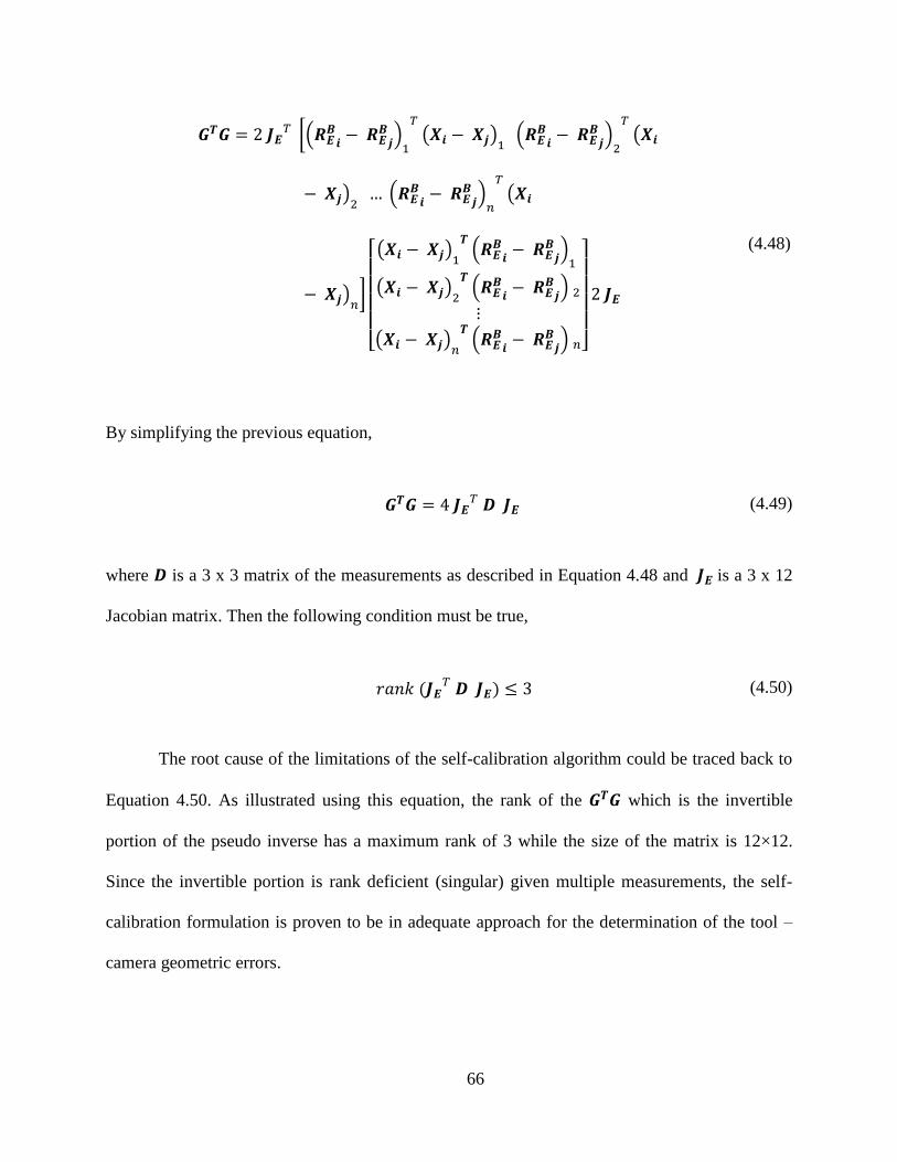
66
[(
)
( ) (
)
(
) (
)
(
) ]
[ ( )
(
)
( ) (
)
( ) (
) ]
(4.48)
By simplifying the previous equation,
(4.49)
where is a 3 x 3 matrix of the measurements as described in Equation 4.48 and is a 3 x 12
Jacobian matrix. Then the following condition must be true,
( ) (4.50)
The root cause of the limitations of the self-calibration algorithm could be traced back to
Equation 4.50. As illustrated using this equation, the rank of the which is the invertible
portion of the pseudo inverse has a maximum rank of 3 while the size of the matrix is 12×12.
Since the invertible portion is rank deficient (singular) given multiple measurements, the self-
calibration formulation is proven to be in adequate approach for the determination of the tool –
camera geometric errors.

67
4.4.3 Off-line Error Measurement for Non-linear Tool Calibration formulation
The robotic tooling self-calibration algorithm is formulated such that the robotic
manipulator has to be moved to different locations in the workspace. The movement is necessary
for the determination of the distances between the holes on the mounted jig. Hence, the robot has
to be operating/on-line during acquiring the measurements for performing the calibration
process.
Contrary to the robotic tooling self-calibration algorithm, the nonlinear tool calibration
formulation developed in section 4.3 has the advantage of being an off-line error measurement
technique. The nonlinear tool calibration algorithm is formulated such that all the measurements
could be acquired using the 3D vision system without moving the robotic manipulator. The
measurements related to the end-effector position as well as the measurements related to the tool
orientation are obtained while the robot is fully static/off-line.
The advantage of the off-line error measurement against the on-line error measurement is
focused in the simplicity of its application. For the tool calibration, the required set-up is limited
to the 3D vision system for digitizing the shapes required in addition to a computer. The data
could be obtained by the user and fed into the calibration algorithm developed for determining
the errors in each axis. The user can then correct the axes that require calibration based on the
tool application. This process could be performed on the workshop floor for multiple robotic
systems with a very short manufacturing down time compared to the current calibration
processes that take a significant time and skill to be performed.

68
CHAPTER 5: MEASUREMENTS SIMULATIONS
This chapter includes all the necessary simulations regarding every aspect of the
measurement process. The simulations in this chapter are not only used to validate the developed
approaches but also for determining the limitations and provide guidance for performing the final
experiments. The first section of this chapter discusses the measurement system which will be
used for obtaining the experimental data. The second and the third sections present the circle
fitting and cylinder fitting methods which will be implemented for performing the tool
calibration. The last two sections of this chapter provide the methodology for determining the
minimum number of data points required during the experiment for achieving the required
accuracy.
5.1 Measurement System
The measurement system used for the experiments is a 3D vision system which is capable
of digitizing any point in the space within its field of vision. The system is 3D Creator FP7000
from Boulder Innovation Group. The system is capable of digitizing any point within 10 meters
field of view with an RMS error of 100 microns. The 3D Creator behaves similar to a Coordinate
Measurement Machine (CMM) but with the advantage of freedom of movement.
The measurement system is composed of two main parts. The first and the main part is
the camera unit, shown in Figure 5-1 below, which includes three line CCD sensors. The second
part accompanied with the system is the hand-held device, shown in Figure 5-2 below. The CCD
line sensors receive infrared light from multiple LED’s located on the hand-held device.

69
\\
The measurement system operates by pointing the red sphere of the hand-held device to
the required point. On pressing the button on the hand-held gun the point is digitized and
captured by the camera unit. The camera unit uses a triangulation method based on the infrared
LEDs and the three CCD sensors for the determination of the point. The point digitized is always
located at the center of the red sphere of the hand-held gun and not at the surface of the sphere.
The 3D vision system specifications are included in Appendix F.
Figure 5-2: Hand-Held Digitizer Gun
Red Sphere
Figure 5-1: Camera Unit
-Z X
Y
CCD
Sensors
3D
vision
frame

70
5.2 End-Effector Position Estimation
The first step of position calibration is the determination of the location of the center of
the robot’s end-effector. The robot’s end-effector shown in Figure 5-3 below is a circular shaped
disk that is designed for mounting the required tool. Using the 3D vision system to determine the
center of the robot’s end-effector, the following process was used.
During the last few decades, there was a need for developing circle fitting methods and
techniques for solving a range of problems in different fields. Physicists use circle fitting
approaches for determining the energy of particles in an accelerator based on diameter of the
circular path of the particles. Recently, in the field of robotics and mobile robotics, it was
necessary to develop algorithms to detect circular objects using the aid of advanced circular laser
systems. The determination of complex curves in computer vision is based on adding multiple
circular arcs together which required developing circle fitting techniques [67].
X
Y
Z
Z
X
Y
End-Effector
Figure 5-3: Robot's End-Effector

71
Many circle fitting techniques were developed which could be mainly divided into two
categories. The first category is the geometric circle fits while the second is the algebraic circle
fits. Unlike the algebraic fits, all the geometric fits use an iterative procedure approach for
improving the fitting accuracy. For complex applications, the normal approach followed for
circle fitting is using an algebraic fit method to determine a good initial guess which is then
followed by using an iterative geometric fit method to improve the accuracy. In general, the
techniques used are mainly dependant on the application and the limitations of the problem.
Algebraic circle fitting techniques are usually simple, reliable and as accurate as
geometric techniques if used under certain conditions. Two algebraic fit techniques were
investigated for determining the center of the robot’s end-effector with respect to the camera
frame. The first technique is a method developed by Bullock [68] called “Least-Squares Circle
Fit”. The method is based on acquiring number of 2D points around the circumference of a circle
in one frame followed by a transformation to different coordinates for solving a minimization
problem. Finally, the solution has to be transformed back into the original coordinates.
The second technique is a simple algebraic fit technique called “Kasa method” [67]. Kasa
method is considered to be the simplest algebraic method for circle fitting. Similar to the
previous method, the Kasa method approach is to minimize the objective function given below,
∑ (5.1)
where
( ) ( ) (5.2)

72
The following step is taking the derivative of the objective function with respect to each
of a, b and r parameters to minimize the errors between the acquired points and the circle
parameters. The derivative of the objective function will lead to nonlinear equations which could
be linearized using simple mathematical manipulation as explained in Appendix B.
The main advantage of the Kasa method in addition to its simplicity and reliability is that
it is capable of determining the exact circle instantly if the measured points lie on the circle.
There are some conditions that need to be taken into consideration for obtaining accurate results
using the Kasa method:
1. The Kasa method was proven to be as accurate as any geometric method if the data
points were taken along the circumference of a full circle. And it was determined to
be significantly inaccurate if the data was taken along a small arc.
2. The data points acquired have to be located very close to the circle. In other words,
the noise in the data points must be very small. The method was proven to provide an
exact geometric results if the noise standard deviation is equal or less than 0.1.
Both methods were tested by generating multiple simulations with different conditions.
The first method was proven to be very sensitive to the location of the data points along the
circle. The second method was proven to be very accurate and adequate for the experiment
conditions. The results for both fitting techniques are shown in the following figures.

73
Table 5-1: Circle Fitting Methods Results
Both of the methods described above require 2D data points for determining the best fit
circle parameters. However, the measurement system described in the previous section provides
the 3D coordinates of any point within its field of vision. As a consequence, an algorithm has to
be developed for fitting a circle in 3D space instead of 2D space.
An algorithm for fitting a circle in 3D space is shown in Figure 5-5. The algorithm starts
by processing 3D data points obtained from the 3D vision system which resemble the shape of a
circle in 3D space. The next step is generating a best fit plane by minimizing the perpendicular
distances between all the points and the plane as explained in Appendix A.
X Y R
Actual Values 3 4 5
Least Square Method 2.9438 4.397 4.988
Kasa Method 2.9999 4.000 4.999
Figure 5-4: Circle Fitting using Kasa Method vs. Least Square Method

74
Afterwards, the 3D points are projected on the best fit plane and an arbitrary frame
attached to the plane is created. The transformation from the camera frame to the plane frame is
determined. Using the transformation, the projected points are transformed from the camera
frame in which the points are 3D to the plane frame in which the points are 2D. The circle fitting
method (Kasa) is used for determining the best fit circle radius and center. Finally, the circle
center is transformed back to the camera frame.
Figure 5-5: 3D Space Circle Fitting Algorithm

75
The 3D circle fitting algorithm developed above along with Kasa method for 2D circle
fitting were verified by simulation. As shown in Figure 5-6 below, circle data point generator
was used to generate multiple data points generally oriented in 3D space. The data points are
shown in Figure 5-6 as blue circular-shaped points. The points were used to generate the best fit
plane which is then used for projecting the points on to it. The projected points are shown as the
blue cross-shaped figures. The circle center was determined and transformed back to the 3D
vision frame as represented by the large red cross-shaped figure.
5.3 Tool Pose Estimation
For performing a full pose tooling calibration, the orientation of the tool must be known.
The tool used in this robot set up as explained in the previous chapters is a pneumatic riveting
Figure 5-6: Simulated 3D Circle Fitting Algorithm

76
gun as shown in Figure 5-7. The main problem is the determination of the orientation of the rivet
gun. The first simple approach that could be used for determining the tool orientation is by
obtaining only two points on the axis of the tool. The two points suggested were the end-effector
center point and the tool center point (TCP). This approach was dismissed because of the
following reasons:
1. The end-effector center point is definitely not on the tool axis due to the position
errors of the tool mount assembly and manufacturing.
2. The tool center point (TCP) is very difficult to be determined accurately since the tool
tip is movable and not rigid.
The second approach which is guaranteed to provide the tool orientation is fitting a
cylinder to the cylindrical shaped rivet gun barrel. Determining the orientation axis of the fitted
cylinder is the same as determining the orientation of the tool. The main idea is to use the 3D
vision system to digitize multiple points on the surface of the rivet gun barrel. Afterwards, an
optimization technique would be used to fit a cylinder shape to the obtained data points. The
Figure 5-7: Pneumatic Rivet Gun

77
orientation of the cylinder axis with respect to the camera represents the orientation of the tool
with respect to the camera.
Cylinder fitting algorithms were researched extensively for determining a simple cylinder
fitting approach. Unfortunately, the problem of fitting a cylinder shape to 3D data points is
considered to be a complicated problem due to the nonlinearity of the cylinder equations in
general orientation in the space. A new method was formulated for cylinder fitting using genetic
algorithm as a search method for determining the best fit cylinder parameters.
5.3.1 Fitness Function
The first step of using genetic algorithm for optimizing the cylinder parameters for
obtaining the best fit cylinder is designing the fitness function. The fitness function is the cost
function which will be minimized by the genetic algorithm by estimating the optimized
parameters.
A generally oriented cylinder in the space could be completely described by seven
parameters. Three parameters of which are used for describing the position of any point on the
cylinder axis. Three more parameters are used for describing the orientation of the axis of the
cylinder. The last parameter is used for describing the radius of the cylinder. The following
assumptions were used for reducing the number of parameters to five,
1. The orientation of the cylinder axis will be described using the spherical coordinates.
The spherical coordinate system uses only two angles which are the polar and
azimuth angles. Using these two angles, the orientation of the cylinder axis could be
easily determined.

78
2. The axis of the cylinder is assumed to be in a general orientation in the space. Hence,
the axis intersects the XY plane as shown in Figure 5-8. As a result, an easy point that
lies on the axis of the cylinder is the intersection point with the XY plane where Z is
equal to zero.
The equations that fully describe a cylinder which is generally oriented in space are given
in Appendix C. The fitness function formulation is based on minimizing the errors between the
radius of the cylinder and the distance from the axis to data points as described by the following
equations,
( ( )) (5.3)
( ) ‖
‖
(5.4)
where is the radius of the cylinder and and are given using the following equations,
( ) ( ) ( ) ( ) ( ) ( ) ( ) (5.5)
( ) ( ) ( ) ( ) (5.6)
X
Y
Z
Cylinder Axis
Intersection Point
Figure 5-8: Cylinder in General Orientation

79
The developed cylinder fitting algorithm was verified by simulating 3D point cloud of a
cylinder generally oriented in space as shown in Figure 5-9 below. The parameters of the
generated data points are given in Table 5-2. The generated data points were used in the GA for
estimating the best fit cylinder parameters. The best fitness value is 1.29647 x 10⁻⁵
, shown in
Figure 5-10, given the GA was set to 500 generations and 500 population size. The GA cylinder
estimated results are tabulated in Table 5-3 below.
Table 5-2: Simulated Cylinder Data Points Parameters
X (mm) Y(mm) Radius (mm) θ (deg) ϕ (deg)
2.60802492 6.12454604 5 30 20
Figure 5-9: Generated Point Cloud and Best Fit Cylinder

80
Table 5-3: Estimated GA Cylinder Parameters
X (mm) Y(mm) Radius (mm) θ (deg) ϕ (deg)
2.60802498 6.12454605 5 30.000012 19.9999937
5.4 End-Effector Simulation
A circular data point generator was created to simulate the measurement data points
around the circumference of the end-effector disk. The simulation requires the number of data
points needed by the user, the circle range which varies from 0 to 2π, the radius of the circle, the
center of the circle before applying any transformation and finally the rotation matrix to
transform the circle to an arbitrary position.
Figure 5-10: Cylinder Fitting GA with 500 Generations and 500 Population
Size

81
The main purpose of this simulation is to test the effect of the number of data points,
obtained randomly around the circumference of the end-effector, on the accuracy of the center
location of the end-effector using the Kasa method for circle fitting. The generator was set to
impose normally distributed noise with a variance of 0.1 to the data points. The variance was
chosen to represent a system with less accuracy than the current used system. The graph in
Figure 5-12 shows the effect of the number of points on the positional accuracy of the circle
center location. The figure clearly shows that the errors drop from approximately 0.24 at 3 points
to less than 0.05 at roughly 15 points.
It is concluded from this simulation that the minimum number of measurement points
required for locating the center of the end-effector disk using the digitizer is 15 points.
Figure 5-11: Circle Simualtion Data Points

82
5.5 Tool Simulation
A cylinder data point generator was created to simulate the 3D point cloud obtained by
the 3D vision system. The generator could simulate a point cloud of a cylinder in a general
orientation in the space. Multiple parameters could be specified using the generator such as the
intersection of the axis of the cylinder with the X and Y plane before rotation. Other parameters
include the radius of the cylinder, the range of the points generated around the cylinder’s
circumference as well as the range along the cylinder’s axis. Also the number of points desired
by the user and the rotation matrix for general placing the cylinder in a general orientation. A
cylinder point cloud shown in Figure 5-13 was generated using 1000 points in a general
orientation, a circumference range of 2π, an axis range from 0 to 5 units and a radius of 5 units.
Normally distributed errors with variance of 0.1 were imposed on the data points to simulate the
inaccuracies of the measurement system.
Figure 5-12: Circle Center Accuracy vs. Number of Points

83
The 3D point was simulated using two different random generators. The first generator is
used to simulate the points around the circumference of the cylinder as well as along its axis.
This random generator must depict the operation of randomly registering points using the 3D
vision system by a user. The generator used for this purpose uses a uniform distribution function.
The second generator is used to create noise for each point of the data cloud. The noise must be
simulated to replicate the accuracy of the 3D vision system. The generator used for creating the
noise uses a normally distributed function. The difference between the two types of generators is
shown in Figure 5-14 below.
The simulation was used to test the number of data points required for acquiring an
accurate cylinder fit using genetic algorithm. The data point generator was used to create a point
cloud for a randomly oriented cylinder. The following step was the execution of genetic
algorithm multiple times for different numbers of data points.
Figure 5-13: Cylinder Point Cloud with Noise

84
The genetic algorithm was tested multiple times before determining the best set of
parameters for the most accurate optimization results. The following results were obtained using
the following set of genetic algorithm parameters which are a population size of 500 and 1000
generations and a stall limit of 1000 generations as well. Three main criteria were used for
verifying the results of the fitting process which are, first the position errors, second is the
orientation errors and finally radius errors. The position errors were determined by computing
the Root Mean Square Position Error (RMSPE) of the point of intersection of the cylinder axis
with the XY plane obtained from the fitting process and from the generated cylinder data points.
The orientation errors were computed by determining the Root Mean Square Orientation Error
(RMSOE) using the two spherical coordinates’ angles θ and ϕ. The radius error was computed
for each set of number of points.
Figure 5-14: Normal Distribution and Uniform Distribution

85
The RMSPE versus the number of points determined from the simulation was plotted as
shown in the Figure 5-15 below,
The RMSPE were noticed to be 0.07 by having only 5 data points. As shown in the
figure, the RMSPE declines to less than 0.01 by increasing the number of data points to about
250 or 300 points and its average stays almost constant up to 1000 points.
Figure 5-15: RMSPE vs. Number of Points
Figure 5-16: RMSOE vs. Number of Points

86
The second criterion which is the RMSOE versus the number of points was plotted as
shown in Figure 5-16.
The RMSOE was noticed to be above 30 with only 5 data points and it dropped sharply
to less than 5 by increasing the data points to 20. It gradually decreases to less than 1 by
increasing the number of points to about 200.
Finally the radius error was plotted versus the number of points as shown in Figure 5-17
below. Similar to the RMSPE trend, the radius sharply reduced from 0.2 to less than 0.02 by
increasing the number of data points from 5 to approximately 250 or 300 points.
The simulation in this section was used to determine the minimum number of data points
required by the user using the 3D vision system to obtain the optimum cylinder fit using genetic
algorithm. A minimum number of 300 data points is required by the user to derive the errors to
zero.
Figure 5-17: Radius Error vs. Number of Points

87
CHAPTER 6: EXPERIMENTS
This chapter is dedicated to present and analyze the experimental application of the
techniques developed in this thesis. The chapter is divided into five sections, two of which
discuss the circle and cylinder fitting techniques while the other three discuss the position,
orientation and full pose calibration respectively. The experiment was conducted based on the
results and conclusions determined from the simulations presented in the previous chapter.
6.1 End-Effector Pose Estimation
The first step performed in the calibration process is locating the robot’s end-effector
position with respect to the camera frame. The process of determining the end-effector’s frame
starts by digitizing the circular end-effector plate. The camera’s hand-held gun was used to
determine multiple data points along the circumference of the end-effector. It was estimated
based on the end-effector position estimation section that the minimum number of points
required for fitting a circle to a number of points uniformly distributed on the circle is 15 points.
For the experiment 58 points were used for ensuring better accuracy circle fitting, hence, better
end-effector position estimation with respect to the camera frame. The data points were plotted
and shown in Figure 6-1 below,

88
The circle fitting algorithm was applied on the experimental data points to determine the
center of the circle. A plane was fitted to the data points; next the points were projected onto the
plane. Finally, a circle that best fits the projected plane points was generated using Kasa method.
The location of the circle center was then transformed back into the camera’s frame. The location
of the end-effector position with respect to the camera frame was tabulated in Table 6-1 below,
Table 6-1: End-Effector Location with Respect to the Camera Frame
X(mm) Y(mm) Z(mm)
0.050797 × 10³
0.006385 × 10³ -1.80183 × 10
3
According to the circle fitting algorithm described in the previous chapter, a frame has to
be randomly constructed on the plane for transforming the data points from the camera frame to
the plane frame. After the fitting process is complete, another frame has to be constructed which
resembles the end-effector’s frame. As explained in chapter 4, the robot’s tool coordinates has its
Figure 6-1: Experimental Circle Data Points (mm)

89
origin at the center of the end-effector plate. The Z axis is perpendicular to the end-effector’s
frame and the X axis is pointing downwards. Since only the center of the end-effector which is
the origin of the frame was determined, an extra point is required for aligning the frame with the
end-effector.
An alignment point located on the X axis of the end-effector’s frame was obtained using
the digitizer. Multiple measurements were taken for the point and an average was obtained. The
X axis was then determined using the origin and the alignment point. Finally, the end-effector
frame was constructed as shown in Figure 6-2 below,
End-Effector Frame Arbitrary Frame
Figure 6-2: End-Effector Center and Frame Determination

90
6.2 Tool Pose Estimation
The following step for performing the calibration process is the determination of the tool
axis orientation and the tool center point location. The tool axis orientation is determined by
obtaining a point cloud of the tool cylinder shape using the digitizer. It was concluded from the
cylinder simulation that the minimum number of points required for obtaining the best cylinder
fit is 300 points. The best cylinder fit was determined based on three criteria which are the
position, orientation and the radius of the cylinder. For the experiment, a point cloud of 549
points, shown in Figure 6-3, were obtained for reducing the effect of noise on the optimization
process.
The next step is using genetic algorithm for optimizing the cylinder parameters for a best
fit to the point cloud. The GA was set to 1000 generations and 500 population size. The results
were obtained and compared to the actual cylinder parameters. The GA did not succeed in
Figure 6-3: Experimental Cylinder Data Points (mm)

91
determining the best fit cylinder for the point cloud. The reason was found to be due to the
position and orientation of the actual cylinder with respect to the camera frame. It was noticed
that the position of the actual cylinder is very far from the camera frame compared to the
simulation. It was also noticed that the cylinder axis orientation with respect to the camera’s XY
plane is close to being parallel. This is contrary to assumptions used for modelling the cylinder
which states that the axis of the cylinder must not be parallel to the XY plane and that axis must
intersect it. It was also verified using the simulation, that the GA does not return acceptable
cylinder parameters values if the position of the cylinder is shifted to beyond 50 mm in any
direction.
A proposed method for solving the given problem is to introduce an intermediate frame
which is close to the data points and creates a better orientation angle with the cylinder axis. As
shown in Figure 6-4, the Intermediate frame is a frame which is closer and better oriented with
respect to the points. The points will be transformed to the intermediate frame where the cylinder
fitting takes place. After the actual frame tool (rivet gun) frame is determined using the best fit
cylinder parameters, the gun frame could be determined with respect to the camera frame using
the following equation,
GP
Figure 6-4: Introducing an Intermediate Frame Diagram
CP
𝑻𝑰𝑪
𝑻𝑮𝑰

92
(5.7)
The intermediate frame position was determined by averaging all the cylinder data points
and using the position of the averaged point as a position vector to the intermediate frame. The
orientation was set to have the same orientation as the end-effector frame with respect to the
camera frame. Genetic Algorithm was used again for fitting a cylinder to the data points with
respect to the intermediate frame. For determining the best fit cylinder, the GA parameters were
experimented with multiple times using 500 generations and different population sizes. The
results could be found in Table 6-2 below,
Table 6-2: Cylinder GA Results with respect to the Intermediate Frame
Population Size X (mm) Y(mm) Radius (mm) θ(deg) ϕ (deg)
100 2.9975 1.7335 17.4392 1.3776 -0.05501
200 2.9976 1.7335 17.4393 0.1932 -0.04609
300 2.9976 1.7334 17.4392 1.9190 -0.06084
400 2.9976 1.7335 17.4393 0.96771 -0.05299
500 2.9976 1.7336 17.4393 -0.11928 -0.04365
The best fitness obtained is 131.784 using 500 Generations and 500 Population size
shown in Figure 6-5. It was noticed that the fitness value does not change using more generations
or bigger population sizes.

93
By observing the results obtained in Table 6-2, it is clearly noticeable that the X and Y
position as well as the Radius are stable and consistent given different population sizes. Unlike
the X, Y and Radius, the angles θ and φ are fluctuating.
For acquiring a stable set of results for the angles, Monte Carlo estimate has to be applied
for stabilizing the angles values. Monte Carlo estimate is a simple averaging method where the
mean value of the estimated parameters is computed over multiple number of GA iterations as
expressed in the following equation,
( )
∑ ( )
(5.8)
Figure 6-5: Cylinder Fitting GA with 500 Generations and 500 Population Size.

94
Table 6-3: Monte Carlo Simulation Results
X Y Radius (mm) θ (deg) ϕ (deg)
2.997638 1.733515 17.439245 1.314285 -0.017301
As shown in Figure 6-6, the obtained values were used to plot the cylinder and the
experimental data points with respect to the intermediate frame.
The cylinder parameters were used to determine the orientation of the tool (rivet gun)
frame with respect to the end-effector. As shown in Figure 6-7, the diagram explains the camera,
end-effector, gun set up with respect to each other. The orientation of the gun frame was
determined with respect to the intermediate frame. The orientation of the end-effector frame was
also determined with respect to the camera frame in the previous section. Using the following set
Figure 6-6: Cylinder Fitting Experimental Point Cloud

95
of equations, the gun frame orientation could be easily determined with respect to the end-
effector frame.
(5.9)
(5.10)
As described previously, the nominal orientation of the rivet gun frame perfectly
matches the orientation of the end-effector frame based on the design CAD models. The
orientation and position of both the measured frame and the nominal frame of the rivet gun with
respect to the end-effector was compared and presented in Table 6-4.
Table 6-4: Measured and Nominal Rotation Matrices and Position Vectors
Rotation Matrix Position Vector (mm)
Measured
0.99973901 0.02287969 0.00313807 50.71440250
0.01369228 -0.49987496 0.86606358 331.20808750
Figure 6-7: Camera, End-Effector and Gun Set-up Diagram
{3D Vision}
{Intermediate}
{End-Effector}
{Gun}
𝑹𝑰𝑪
𝑹𝑬𝑽
𝑹𝑮𝑬
𝑹𝑮𝑰

96
0.01864527 -0.86578654 -0.49992601 -1980.231250
Nominal
0.99963924 0.02683525 0.00171706 51.433657
0.01393145 -0.48241207 0.87586855 330.970868
0.02296312 -0.87552865 -0.48254672 -1980.661388
6.3 Linear Full Pose Calibration
By determining the tip pose errors using the nominal and the measured transformation of
the tool frame with respect to the end-effector frame, the linear formulation for full pose
calibration can be applied. As shown in Figure 6-8, the root mean square error (RMSE)
converges from the value of approximately 3 to 1 × 10⁻⁴
in only 4 iterations. The tool position
and orientation geometric error is presented in Table 6-5. The calibrated rotation matrix and the
position vector is also presented in Table 6-6 below.
Figure 6-8: Linear Calibration RMSE vs. Number of Iterations

97
Table 6-5: Linear Formulation Estimated Geometric Errors
Δx(mm) Δy(mm) Δz(mm) δx(deg) δy (deg) δz(deg)
-0.705815564 -0.510370452 0.000462561 -1.144895889 0.055203477 0.223368453
Table 6-6: Calibrated Tool Pose Rotation Matrix and Position Vector
Rotation Matrix Position Vector (mm)
Calibrated
0.998908940 0.046707348 -0.001020997 51.040929326
0.025909742 -0.481775206 0.875946652 331.237715206
0.039052347 -0.875044604 -0.482390830 -1980.175216802
6.4 Nonlinear Position Calibration
Using the measured and the nominal rivet gun frames results determined in the last
section, the first nonlinear calibration process that will be applied is the position only calibration.
The aim of this calibration is to correct the errors related to the position by excluding the
orientation parameters from the fitness function.
The GA parameters were set to have 500 Generations and 100 Population size. The best
fitness value determined under these conditions as shown in Figure 6-9 is 1.54239 × 10⁻⁷
. The
position errors determined from the calibration process are tabulated in Table 6-7.
Table 6-7: Position Errors
ΔX (mm) ΔY (mm) ΔZ (mm)
-0.705815507 -0.51034175499 0.00097941593

98
The position error was added to the nominal position vector to obtain the calibrated
position vector presented in Table 6-8 below.
Table 6-8: Calibrated Position
X (mm) Y (mm) Z (mm)
50.714403336 331.2080880877 -1980.231250049
6.5 Nonlinear Orientation Calibration
The next calibration process if the orientation only calibration which will be performed
based on the nominal and measured rotation matrices of the rivet gun frame with respect to the
camera’s frame. By setting the weight factor of the position to zero and the weight factor of the
orientation to one, the algorithm excludes the position parameters from the fitness function.
Figure 6-9: Position Only Calibration with 500 Generations and 100 Population
Size

99
The genetic algorithm parameters were set to multiple values for determining the best
performance. The first trial was to assign the GA to run for 500 Generations and use a population
size of 100. The fitness value determined based on these conditions is 0.00141989 as shown in
Figure 6-10 below.
The orientation errors δx, δy and δz values obtained from this calibration process are
presented in Table 6-9 below,
Table 6-9: Orientation Errors for 500 Generations and 100 Population Size
δx (deg) δy(deg) δz(deg)
-1.14584428 -0.02608992 0.22273761
Figure 6-10: Orientation Only Calibration with 500 Generations and 100
Population Size

100
Using the orientation errors in the Table above, the calibrated rotation matrix was
calculated and tabulated in Table 6-10 below along with the measured and the nominal rotation
matrices for comparison.
Table 6-10: Measured, Nominal and Calibrated Rotation Matrices with respect to the Camera frame
Rotation Matrix
Measured
0.99973901 0.02287969 0.00313807
0.01369228 -0.49987496 0.86606358
0.01864527 -0.86578654 -0.49992601
Nominal
0.99963924 0.02683525 0.00171706
0.01393145 -0.48241207 0.87586855
0.02296312 -0.87552865 -0.48254672
Calibrated
0.99973669 0.02291913 0.00172049
0.01245480 -0.49988111 0.86603981
0.01933960 -0.86578634 -0.49996905
Since the rivet gun frame was designed to be perfectly aligned with the end-effector’s
frame with nominal angles of zeros, the calibrated values is the summation of the nominal values
and the orientation errors presented in Table 6-10 above. As a result the calibrated angles are the
same as the orientation errors.
The second trial of the orientation calibration was performed by increasing the number of
the population size to 300 while maintaining the same number of 500 generations. It was
observed that the best fitness value is the same as the previous trial and it stays constant as
shown in Figure 6-11, even in the case of increasing the population size or the number of
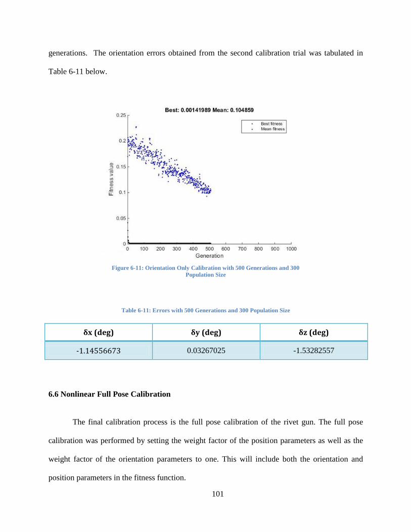
101
generations. The orientation errors obtained from the second calibration trial was tabulated in
Table 6-11 below.
Table 6-11: Errors with 500 Generations and 300 Population Size
δx (deg) δy (deg) δz (deg)
-1.14556673 0.03267025 -1.53282557
6.6 Nonlinear Full Pose Calibration
The final calibration process is the full pose calibration of the rivet gun. The full pose
calibration was performed by setting the weight factor of the position parameters as well as the
weight factor of the orientation parameters to one. This will include both the orientation and
position parameters in the fitness function.
Figure 6-11: Orientation Only Calibration with 500 Generations and 300
Population Size

102
Multiple trials were performed for obtaining the best full pose calibration performance.
The GA parameters were set to 500 Generations and 100, 300 and 500 population sizes. The best
fitness values corresponding to each of the population sizes are 0.00172163, 0.00142031 and
0.00141994 respectively. The results are shown in Figures 6-12, 6-13 and 6-14 below.
The position and orientation errors as well as the calibrated rotation matrix and the
position vector are tabulated in Tables 6-12 and 6-13.
Table 6-12: Position and Orientation Errors Based on 500 Generations and 100 Population Size
Δx(mm) Δy(mm) Δz(mm) δx(deg) δy (deg) δz(deg)
-0.70577135 -0.51034633 0.00101015 -1.11740481 -0.03275695 0.24175341
Figure 6-12: Full Pose Calibration with 500 Generations and 100 Population Size

103
Table 6-13: Calibrated Rotation Matrix and Position Vector Based on 500 Generations and 100 Population size
Rotation Matrix Position Vector
Calibrated
0.99974439 0.02259051 0.00158633 50.71444665
0.01239659 -0.49945512 0.86628639 331.20811731
0.01899284 -0.86604080 -0.49954145 -1980.23125971
Table 6-14: Position and Orientation Errors with 500 Generations and 300 Population Size
Δx(mm) Δy(mm) Δz(mm) δx(deg) δy (deg) δz(deg)
-0.70581548 -0.51034168 0.00097945 -1.14641395 -0.02608559 0.22055166
Figure 6-13: Full Pose Calibration with 500 Generations and 300 Population Size

104
Table 6-15: Calibrated Rotation Matrix and Position Vector Based on 500 Generations and 300 Population Size
Rotation Matrix Position Vector
Calibrated
0.99973581 0.02295725 0.00172156 50.71440262
0.01247314 -0.49988926 0.86603485 331.20808756
0.01937304 -0.86578062 -0.49997766 -1980.23124998
Table 6-16: Position and Orientation Errors with 500 Generations and 500 Population Size
Δx(mm) Δy(mm) Δz(mm) δx(deg) δy (deg) δz(deg)
-0.70581560 -0.51034164 0.00097941 -1.14692394 -0.02608552 0.22104372
Figure 6-14: Full Pose Calibration with 500 Generations and 500 Population Size

105
Table 6-17: Calibrated Rotation Matrix and Position Vector Based on 500 Generations and 500 Population Size
Rotation Matrix Position Vector
Calibrated
0.99973601 0.02294865 0.00172159 50.71440250
0.01246900 -0.49989707 0.86603040 331.20808750
0.01936553 -0.86577634 -0.49998537 -1980.23125000
It was observed that the best fitness does not decrease below 0.00141994 by increasing
the population sizes above 500 neither by increasing the number of generations above 500.

106
CHAPTER 7: CONCLUSION, CONTRIBUTIONS AND FUTURE WORK
7.1 Conclusion
Robotic Tooling Calibration is a very critical step in the automation process of
manufacturing especially during the tasks that require high level of accuracy. Different tool
calibration methods were investigated and developed in this thesis. First, the system required for
the calibration method was designed for considering more than one calibration approach. The
first formulation considered for the tooling calibration is the linear formulation. The linear
formulation was extensively studied by developing two approaches; the first is based on the
conventional calibration using least squares, while the second is based on self-calibration
formulation. The linear method based on self-calibration was analyzed and proven to be an
unsuccessful approach for tool calibration due to Jacobian rank deficiency. The conventional
calibration formulation was analyzed and implemented on the experimental data. The second
formulation for determining the errors as well as calibrating the tool is the nonlinear approach. A
nonlinear formulation was developed in this thesis using genetic algorithm as a search method
for determining the tool errors. The method was simulated and the limitations regarding the end-
effector position and the tool orientation estimation were determined. The method was applied
on the experimental data obtained from the actual robot system set-up and the errors were
identified and the tool geometric parameters were calibrated.
7.2 Contributions
The contributions that were provided in this thesis could be summarized in the following points,

107
1. A robotic tooling calibration approach was developed based on a nonlinear approach
using genetic algorithm. The developed method is robust and simple to apply in a
manufacturing environment. The method uses an off-line error measurement
approach which does not require any robot movements and reduces the down time of
the manufacturing line.
2. The linear formulation based on the self-calibration formulation was analyzed. The
root causes of the ineffectiveness of the linear formulation based on self-calibration
algorithm was determined and discussed. The causes are traced back to the Jacobian
rank deficiency.
3. The Linear formulation based on the conventional calibration, using least squares,
was analyzed and implemented on the experimental data.
4. A tool orientation estimation method was developed in this thesis to accurately
measure the tool orientation. The method was developed by formulating a cylinder
fitting algorithm which uses genetic algorithm for determining all the cylinder’s
parameters.
7.3 Future Work
Robotic tooling calibration is a crucial topic which requires a lot of research for covering
all of its different aspects. Several recommendations are provided below based on the research
conducted in this thesis for future work.

108
First, the tool geometric errors obtained from both the linear formulation approach as
well as the nonlinear formulation should be implemented for tool calibration. In other words, the
errors determined should be inserted into the robot’s controller. Multiple tests have to be
conducted to determine whether the robot can be commanded to successfully insert a rivet into a
predetermined hole.
Second, the robot was considered to be calibrated before tool calibration takes place.
However, the effects of the tool weight on the accuracy of the robotic manipulator are eminent
and should be extensively studied. A tool calibration model should be developed to account for
the robot manipulator errors due to the tool weight.
Third, the method developed in this thesis could be expanded to include the calibration of
the robotic manipulator as well. By locating the tool tip pose and the vision system location with
respect to the base frame, a formulation could be developed for including the robot geometric
parameters errors. Also a study has to be conducted to determine the effects and contribution of
the robot geometric errors to the tool tip errors.
Fourth, the orientation estimation of different tool shapes must be considered. Different
shapes fitting techniques must be developed for determining the location of different types of
tools. Also, a laser scanner measurement tool is considered to be more appropriate for
determining more complex shapes. For accurately determining the shape of a cylinder, around
300 points were required. Using a laser scanner could significantly provide a lot of points in a
short period of time.

109
LIST OF APPENDICES
APPENDIX A – PLANE FITTING
The equation of a plane could be described using the following equations,
(A.A.1)
By reordering the terms,
(A.A.2)
Minimizing the distance between the plane and the points using the following equations,
( ) (A.A.3)
∑( ( )) (A.A.4)
Figure A-1: Best Fit Plane Generated for Multiple Points

110
APPENDIX B – KASA METHOD
A circle in a 2D plane could be expressed using the following equation,
( ) ( )
(A.B.1)
By minimizing the errors between the points and the edge of the circle given the following
equation,
( ) ( )
(A.B.2)
By taking the derivative of the function above and linearizing the parameters using the
following,
(A.B.3)
By expanding Equation A.6 and substituting the values in Equation A.7,
(A.B.4)
(
) (A.B.5)
(A.B.6)
(∑ ) (A.B.7)
Equation (A.B.7) is done by taking the differentiation with respect to B, C and D and then
solving the system of equations. The parameters of the circle could be easily obtained using the
following equations,
√
(A.B.8)

111
APPENDIX C– CYLINDER EQUATIONS
A cylinder that has its axis aligned with the Z-axis of a frame 2 could be expressed using
the following equations,
( ) (A.C.1)
( ) (A.C.2)
(A.C.3)
For expressing a general orientation cylinder the following sequence of rotations must be
applied as shown in Figure A-2 and described in the following equations,
(A.C.4)
where
( ) [
] (A.C.5)
( ) [
] (A.C.6)
( ) ( ) [
] (A.C.7)
The cylinder equations expressed above could be transformed using the following equation,
[ ]
[ ] (A.C.8)

112
[ ] [
] [ ] (A.C.9)
( ) ( ) ( ) ( ) ( ) (A.C.10)
( ) ( ) (A.C.11)
( ) ( ) ( ) ( ) ( ) (A.C.12)
1
2 3
Figure A-2: Cylinder Rotation Sequence

113
APPENDIX D – ROBOT END-EFFECTOR IN BASE FRAME
The robot’s end-effector pose with respect to the base frame could be easily obtained
from the robot’s controller as presented in Table A-1 below. Using the parameters obtained from
the controller, the homogeneous transformation from the end-effector to the base frame could be
calculated as presented in Table A-2 below.
Table A-1: End-Effector Parameters with respect to the Base Frame
X Y Z EZ EY EX
1150.8 28.7 1324.9 0 90 0
Table A-2: Rotation Matrix and Position Vector of the End-Effector with respect to the Base Frame
Rotation Matrix Position Vector
(mm)
0 1 0 1150.8
0 0 1 28.7
-1 0 0 1324.9
APPENDIX E – JACOBIAN MATRIX
The calculated Jacobian Matrix ,
[ ]

114
APPENDIX F – 3D VISION SYSTEM

115

116
REFERENCES
[1] Wallén, J. (2008). The history of the industrial robot. Technical Report from Automatic
Control at Linkopings University, Linkoping, Sweden.
[2] Craig, J. J. (2005). Introduction to robotics: mechanics and control Vol. 3. Upper Saddle
River: Pearson Prentice Hall.
[3] Lin, Y. (2008). Robot calibration based on nonlinear formulation for modular
reconfigurable robots (MRRS) (Master’s Thesis). Ryerson University. School of
Graduate Studies. Program of Mechanical Engineering.
[4] Schneider, U., Ansaloni, M., Drust, M., Leali, F., & Verl, A. (2013). Experimental
Investigation of Sources of Error in Robot Machining. In Robotics in Smart
Manufacturing (pp. 14-26). Berlin: Springer.
[5] Khalil, W., & Dombre, E. (2004). Modeling, identification and control of robots. Oxford:
Butterworth-Heinemann.
[6] Everett, L., Driels, M., & Mooring, B. (1987). Kinematic modelling for robot calibration.
In IEEE International Conference on Robotics and Automation. Proceedings. Vol. 4, pp.
183–189.
[7] Denavit, J. (1955). A kinematic notation for lower-pair mechanisms based on matrices.
Trans. of the ASME. Journal of Applied Mechanics, 22, 215–221.
[8] Paul, R. P., & Shimano, B. (1979). Kinematic control equations for simple manipulators.
In IEEE Conference on Decision and Control including the 17th Symposium on Adaptive
Processes, pp. 1398-1406.
[9] Ibarra, R., & Perreira, N. D. (1985). Determination of Linkage Parameter and Pair
Variable Errors in Open Chain Kinematic Linkages Using a Minimal Set of Position

117
Measurement Data. ASME Paper, 85-DET, 51.
[10] Wu, C. (1984). A Kinematic CAD tool for the design and control of a robot manipulator.
The International Journal of Robotics Research, 3(1), 58–67.
[11] Wu, C. H. (1983). The kinematic error model for the design of robot manipulator.
In IEEE on American Control Conference, pp. 497-502.
[12] Zhen, H. (1985). Error analysis of robot manipulators and error transmission functions.
Proc. of the 15th ISIR, Tokyo, pp. 873–878.
[13] Payannet, D., Aldon, M. J., & Liegeois, A. (1985). Identification and compensation of
mechanical errors for industrial robots. Proc.15th Int.Symp.on Industrial Robots, 857–
864.
[14] Mooring, B. W. (1983). The effect of joint axis misalignment on robot positioning
accuracy. Proceedings of the ASME International Computers in Engineering Conference,
151–156.
[15] Hayati, S. A. (1983). Robot arm geometric link parameter estimation. In The 22nd IEEE
Conference on Decision and Control, 1983. Vol. 22, pp. 1477–1483.
[16] Mooring, B. W., Roth, Z. S., & Driels, M. R. (1991). Fundamentals of manipulator
calibration. Toronto: John Wiley & Sons, Inc.
[17] Hayati, S. A., & Mirmirani, M. (1984). A software for robot geometry parameter
estimation. In Robots West Conference, Anaheim, California.
[18] Stone, H., Sanderson, A., & Neuman, C. (1986). Arm signature identification. In IEEE
International Conference on Robotics and Automation. Proceedings. Vol. 3, pp. 41–48.
[19] Hsu, T. W. (1987). Robot accuracy improvement through kinematic parameter
identification (Doctoral dissertation). ProQuest, UMI Dissertation Publishing.

118
[20] Paul, R. P. (1981). Robot manipulators: mathematics, programming, and control : the
computer control of robot manipulators. Cambridge: MIT Press.
[21] Whitney, D. E., Lozinski, C. A., & Rourke, J. M. (1986). Industrial robot forward
calibration method and results. Journal of Dynamic Systems, Measurement, and Control,
108(1), 1–8.
[22] Hollerbach, J. M. (1989). A survey of kinematic calibration. In The robotics review 1, pp.
207-242. Cambridge: MIT Press.
[23] Chen, J., & Chao, L.-M. (1987). Positioning error analysis for robot manipulators with all
rotary joints. IEEE Journal on Robotics and Automation, 3(6), 539–545.
[24] Gatla, C. S., Lumia, R., Wood, J., & Starr, G. (2007). An automated method to calibrate
industrial robots using a virtual closed kinematic chain. Robotics, IEEE Transactions on
Robotics, 23(6), 1105-1116.
[25] Lightcap, C., Hamner, S., Schmitz, T., & Banks, S. (2008). Improved positioning
accuracy of the PA10-6CE robot with geometric and flexibility calibration. IEEE
Transactions on Robotics, 22(2), 452–456.
[26] Yurttagul, B. (2010). Kinematic calibration of industrial robots using full pose
measurements and optimal pose selection. Ankara, Turkey: METU.
[27] Joubair, A., Nubiola, A., & Bonev, I. (2013). Calibration efficiency analysis based on
five observability indices and two calibration models for a six-axis industrial robot. SAE
International Journal of Aerospace, 6(1), 161–168.
[28] Doebelin, E. O. (2004). Measurement systems: application and design. Boston:
McGraw-Hill.
[29] Gong, C., Yuan, J., & Ni, J. (2000). Nongeometric error identification and compensation

119
for robotic system by inverse calibration. International Journal of Machine Tools and
Manufacture, 40(14), 2119–2137.
[30] Majarena, A. C., Santolaria, J., Samper, D., & Aguilar, J. J. (2011). Modelling and
calibration of parallel mechanisms using linear optical sensors and a coordinate
measuring machine. Measurement Science and Technology, 22(10), 105101.
[31] Meng, G., Tiemin, L., & Wensheng, Y. (2003). Calibration method and experiment of
Stewart platform using a laser tracker. In IEEE International Conference on Systems,
Man and Cybernetics, Vol. 3, pp. 2797-2802.
[32] TP200 co-ordinate measuring machines, photograph (2012), Retrieved 29 May 2015,
http://www.th.all.biz/img/th/catalog/32617.jpeg.
[33] Mooring, B. W., & Padavala, S. S. (1989). The effect of kinematic model complexity on
manipulator accuracy. In IEEE International Conference on Robotics and Automation.
Proceedings, pp. 593-598.
[34] Zhuang, H., Wang, L. K., & Roth, Z. S. (1993). Error-model-based robot calibration
using a modified CPC model. Robotics and Computer Integrated Manufacturing, 10(4),
287–299.
[35] Cooper, M. A. R. (1982). Modern theodolites and levels. Oxford: BSP Professional
Books.
[36] Remy, S., Dhome, M., Lavest, J. M., & Daucher, N. (1997). Hand-eye calibration.
In Proceedings of the IEEE/RSJ International Conference on Intelligent Robots and
Systems, Vol. 2, pp. 1057-1065.
[37] Motta, J. M. S. T., Carvalho, G. C. de, & McMaster, R. S. (2001). Robot calibration using
a 3D vision-based measurement system with a single camera. Robotics and Computer

120
Integrated Manufacturing, 17(6), 487–497.
[38] Visual servoing: uncalibrated hand-eye coordination through differential visual feedback,
photograph, viewed 20 May 2015,
https://www.cs.rochester.edu/u/jag/PercAct/dvfb.html.
[39] Pathre, U. S., & Driels, M. R. (1990). Simulation experiments in parameter identification
for robot calibration. The International Journal of Advanced Manufacturing Technology,
5(1), 13–33.
[40] Siciliano, B., & Khatib, O. (2008). Springer handbook of robotics. Stanford: Springer
Science & Business Media.
[41] Levenberg, K. (1944). A method for the solution of certain non-linear problems in least
squares. Quarterly Journal of Applied Mathmatics, II (2), 164–168.
[42] Marquardt, D. W. (1963). An algorithm for least-squares estimation of nonlinear
parameters. Journal of the Society for Industrial and Applied Mathematics, 11(2), 431–
441.
[43] Chao, L. M., & Yang, J. C. S. (1986). Development and implementation of a kinematic
parameter identification technique to improve the positioning accuracy of robots. Society
of Manufacturing Engineers.
[44] Judd, R. P., & Knasinski, A. B. (1990). A technique to calibrate industrial robots with
experimental verification. IEEE Transactions on Robotics and Automation, 6(1), 20–30.
[45] Gan, Y., & Dai, X. (2011). Base frame calibration for coordinated industrial robots.
Robotics and Autonomous Systems, 59(7), 563–570.
[46] Wang, H., Shen, S., & Lu, X. (2012). A screw axis identification method for serial robot
calibration based on the POE model. Industrial Robot: An International Journal, 39(2),

121
146–153.
[47] Lin, Y., Xi, F., Mohamed, R., & Tu, X. W. (2010). Calibration of modular reconfigurable
robots based on a hybrid search method. Journal of manufacturing science and
engineering, 132(6), 061002.
[48] Zhuang, H., Wang, K., & Roth, Z. S. (1994). Optimal selection of measurement
configurations for robot calibration using simulated annealing. In IEEE International
Conference on Robotics and Automation, pp. 393-398.
[49] Sun, Y., & Hollerbach, J. M. (2008). Observability index selection for robot calibration.
In IEEE International Conference on Robotics and Automation, pp. 831-836.
[50] Driels, M. R., & Pathre, U. S. (1990). Significance of observation strategy on the design
of robot calibration experiments. Journal of Robotic Systems, 7(2), 197–223.
[51] Watanabe, A., Sakakibara, S., Ban, K., Yamada, M., Shen, G., & Arai, T. (2006). A
Kinematic Calibration Method for Industrial Robots Using Autonomous Visual
Measurement. CIRP Annals - Manufacturing Technology, 55(1), 1–6.
[52] Khalil, W., Besnard, S., & Lemoine, P. (2000). Comparison study of the geometric
parameters calibration methods. International Journal of Robotics and
Automation, 15(2), pp-56.
[53] Gong, C., Yuan, J., & Ni, J. (2000). A Self-Calibration Method for Robotic Measurement
System. Journal of Manufacturing Science and Engineering, 122(1), 174.
[54] Zhuang, H., Motaghedi, S. H., & Roth, Z. S. (1999). Robot calibration with planar
constraints. In IEEE International Conference on Robotics and Automation. Vol. 1, pp.
805-810.
[55] Dornaika, F., & Horaud, R. (1998). Simultaneous robot-world and hand-eye calibration.

122
IEEE Transactions on Robotics and Automation, 14(4), 617–622.
[56] Zhan, Q., & Wang, X. (2012). Hand–eye calibration and positioning for a robot drilling
system. The International Journal of Advanced Manufacturing Technology, 61(5), 691–
701.
[57] Wang, H., Fan, X., & Lu, X. (2013). Application of a hand-eye self-calibration technique
in robot vision. In Control and Decision Conference (CCDC), 25th Chinese on pp. 3765-
3769.
[58] Axelrod, B., & Huang, W. H. (2012). Improving hand-eye calibration for robotic
grasping and manipulation. In IEEE International Conference on Technologies for
Practical Robot Applications (TePRA), 2012 pp. 121-126.
[59] Hallenberg, J. (2007). Robot tool center point calibration using computer vision
(Master’s Thesis). Linköping, Sweden: University of Linkoping.
[60] Ayadi, A., Nicolau, S., Bayle, B., Graebling, P., & Gangloff, J. (2007). Fully automatic
needle calibration for robotic-assisted puncture on small animals. In IEEE/NIH on Life
Science Systems and Applications Workshop, pp. 85–88.
[61] Cheng, F. S. (2007). The method of recovering robot TCP positions in industrial robot
application programs. In International Conference on Mechatronics and Automation. pp.
805-810.
[62] Shiu, Y. C., & Ahmad, S. (1989). Calibration of wrist-mounted robotic sensors by
solving homogeneous transform equations of the form AX=XB. IEEE Transactions on
Robotics and Automation, 5(1), 16–29.
[63] Park, F. C., & Martin, B. J. (1994). Robot sensor calibration: solving AX=XB on the
Euclidean group. IEEE Transactions on Robotics and Automation, 10(5), 717–721.

123
[64] Zuang, H., & Shiu, Y. C. (1993). A noise-tolerant algorithm for robotic hand-eye
calibration with or without sensor orientation measurement. IEEE Transactions on
Systems, Man, and Cybernetics, 23(4), 1168–1175.
[65] Daniilidis, K. (1999). Hand-eye calibration using dual quaternions. The International
Journal of Robotics Research, 18(3), 286–298.
[66] Helal, M., Xi, F., & Lin, Y. (2013). Robotic Tooling Self-Calibration. SAE Technical
Paper. (No. 2013-01-2118).
[67] Chernov, N. (2010). Circular and linear regression: fitting circles and lines by least
squares. Florida: CRC Press.
[68] Bullock, R., 2006. Least-Squares Circle Fit. Retrieved 29 May 2015,
http://www.dtcenter.org/met/users/docs/write_ups/circle_fit.pdf.
[69] Xi, F., Lin, Y., Dakdouk, D., Helal, M., & East, B. (2013). Patent No. WO 2013152440
A1. Canada.
[70] Holland, J. H. (1975). Adaptation in natural and artificial systems: an introductory
analysis with applications to biology, control, and artificial intelligence. Oxford,
England: U Michigan Press.
[71] McMaster, R., & Ribeiro, F. M. (1994). Cell calibration and robot tracking. In Next Steps
for Industrial Robotics, IEE Colloquium on pp. 3-1.