Robots Are Us: Some Economics of Human

Replacement∗

Seth G. Benzell1, Laurence J. Kotlikoff1, Guillermo LaGarda1, andJeffrey D. Sachs2

1Department of Economics, Boston University2The Earth Institute, Columbia University

March 29, 2015

Abstract

Will smart machines replace humans like the internal combustion engine replacedhorses? If so, can putting people out of work, or at least out of good work, alsoput the economy out of business? Our model says yes. Under the right conditions,more supply produces, over time, less demand as the smart machines undermine theircustomer base. Highly tailored skill- and generation-specific redistribution policiescan keep smart machines from immiserating humanity. But blunt policies, such asmandating open-source technology, can make matters worse.

∗We would like to thank Dilip Mookherjee, Dietrich Vollrath, and Kevin Cooke for theiruseful comments.

1 Introduction

Whether it’s bombing our enemies, steering our planes, fielding our calls, rub-bing our backs, vacuuming our floors, driving our taxis, or beating us at Jeop-ardy, it’s hard to think of hitherto human tasks that smart machines can’t door won’t soon do. Few smart machines look even remotely human. But theyall combine brains and brawn, namely sophisticated code and physical capital.And they all have one ultimate creator – us.

Will human replacement - the production by ourselves of ever better substitutesfor ourselves - deliver an economic utopia with smart machines satisfying ourevery material need? Or will our self-induced redundancy leave us earning toolittle to purchase the products our smart machines can make?

Ironically, smart machines are invaluable for considering what they might doto us and when they might do it. This paper uses the most versatile of smartmachines – a run-of-the-mill computer – to simulate one particular vision of hu-man replacement. Our simulated economy – an overlapping generations model– is bare bones. It features two types of workers consuming two goods for twoperiods. Yet it admits a large range of dynamic outcomes, some of which arequite unpleasant.

The model’s two types of agents are called high-tech workers and low-tech work-ers. The first group has a comparative advantage at analytical tasks, the sec-ond in empathetic and interpersonal tasks. Both work full time, but only whenyoung. High-tech workers produce new software code, which adds to the ex-isting stock of code. They are compensated by licensing their newly producedcode for immediate use and by selling rights to its future use. The stock of code– new plus old – is combined with the stock of capital to produce automatablegoods and services (hereafter referred to as ‘goods’). Goods can be consumedor used as capital. Unlike high-tech workers, low-tech workers are right brainers– artists, musicians, priests, astrologers, psychologists, etc. They produce themodel’s other good, human services (hereafter referred to as ‘services’). The ser-vice sector does not use capital as an input, just the labor of high and low-techworkers.

Code references not just software but, more generally, rules and instructionsfor generating output from capital. Because of this, code is both created byand is a substitute for the analytical labor provided by high-tech workers inthe good (autmomatable) sector. Code is not to be thought of as accumulatingin a quantitative way (anyone who has worked on a large software project cantestify that fewer lines of code often mean a better program) but rather inefficiency units. Code accumulation may be a result of programmers typing outcode directly, of machine learning systems getting better at a task under thesupervision of human trainers1, or of innovation in designing learning algorithms

1Astro Teller, Google’s ‘Director of Moonshots’, discusses in Madrigal (2014) the impor-tance of this work to Google’s current projects:

Many of Google’s famously computation driven projects—like the creation ofGoogle Maps—employed literally thousands of people to supervise and correctautomatic systems. It is one of Google’s open secrets that they deploy human

1

themselves. In the United States, more than 5 percent of total wages is paid tothose engaged in computer or mathematical occupations2; a much larger shareof compensation is being paid to those engaged in creating code broadly defined.

Code needs to be maintained, retained, and updated. If the cost of doing sodeclines via, for example, the invention of the silicon chip, the model deliversa tech boom, which raises the demand for new code. The higher compensationreceived by high-tech workers to produce this new code engenders more nationalsaving and capital formation, reinforcing the boom. But over time, as the stockof legacy code grows, the demand for new code and, thus for high-tech workers,falls.

The resulting tech bust reflects past humans obsolescing current humans. Thisprocess explains the choice of our title, Robots Are Us. The combination ofcode and capital that produce goods constitutes, in effect, smart machines, akarobots. And these robots contain the stuff of humans – accumulated brain andsaving power. Take Junior – 2013’s World Computer Chess Champion. Juniorcan beat every current and, possibly, every future human on the planet. Con-sequently, his old code has largely put new chess programmers out of business.

Once begun, the boom-bust tech cycle can continue if good producers switchtechnologies a la Zeira (1998) in response to changes over time in the relativecosts of code and capital. But whether or not such Kondratieff waves materi-alize, tech busts can be tough on high-tech workers. In fact, high-tech workerscan start out earning far more than low-tech workers, but end up earning farless.

Furthermore, robots, captured in the model by more code-intensive good pro-duction, can leave all future high-tech workers and, potentially, all future low-tech workers worse off. In other words, technological progress can be immiserat-ing. This finding echoes that of Sachs and Kotlikoff (2012). Although our paperincludes different features from those in Sachs and Kotlikoff (2012), includingtwo sectors, accumulating code stocks, endogenous technological change, prop-erty rights to code, and boom-bust cycle(s), the mechanism by which bettertechnology can undermine the economy is the same. The eventual decline inhigh-tech worker and, potentially, low-tech worker compensation limits whatthe young can save and invest. This means less physical capital available fornext period’s use. It also means that good production can fall over time eventhough the technological capacity to produce goods expands.

The long run in such cases is no techno-utopia. Yes, code is abundant. Butcapital is dear. And yes, everyone is fully employed. But no one is earning verymuch. Consequently, there is too little capacity to buy one of the two things,

intelligence as a catalyst. Instead of programming in that last little bit of relia-bility, the final 1 or 0.1 or 0.01 percent, they can deploy a bit of cheap humanbrainpower. And over time, the humans work themselves out of jobs by teach-ing the machines how to act. “When the human says, ‘Here’s the right thing todo,’ that becomes something we can bake into the system and that will happenslightly less often in the future,” Teller said.

2This figure is the share of wages paid to workers in Computer or Mathematical Occupa-tions in the May 2013 NAICS Occupational Employment and Wage Estimates.

2

in addition to current consumption, that today’s smart machines (our model’snon-human dependent good production process) produce, namely next period’scapital stock. In short, when smart machines replace people, they eventuallybite the hands of those that finance them.

These findings assume that code is excludable and rival in its use. But we alsoconsider cases in which code is non-excludable, non-rival, or both. Doing sorequires additional assumptions but lets us consider the requirement that allcode be open source, i.e., non-excludable. Surprisingly, such freeware policiescan worsen long-run outcomes.

Our paper proceeds with some economic history – Ned Ludd’s quixotic waron machines and the subsequent Luddite movement. As section 2 indicates,Ludd’s instinctive fear of technology, ridiculed for over a century, is now theobject of a serious economic literature. Section 3 places our model within abroader framework of human competition with robots to indicate what we,for parsimony’s sake, exclude. Section 4 presents our model and its solutionmethod. Section 5 illustrates the surprising range of outcomes that even thissimple framework can generate. Section 6 considers how the nature of codeownership and rivalry affects outcomes. Section 7 follows Zeira (1998) in lettingthe choice of production technique respond to relative scarcity of inputs, in ourcase capital and code. Section 8 considers potential extensions of the model toencompass the broader range of factors and frameworks outlined in Section 3.Section 9 concludes.

2 Background and Literature Review

Concern about the downside to new technology dates at least to Ned Ludd’sdestruction of two stocking frames in 1779 near Leichester, England. Ludd,a weaver, was whipped for indolence before taking revenge on the machines.Popular myth has Ludd escaping to Sherwood Forest to organize secret raidson industrial machinery, albeit with no Maid Marian.

More than three decades later – in 1812, 150 armed workers – self-named Lud-dites – marched on a textile mill in Huddersfield, England to smash equipment.The British army promptly killed or executed 19 of their number. Later thatyear the British Parliament passed The Destruction of Stocking Frames, etc.Act, authorizing death for vandalizing machines. Nonetheless, Luddite riotingcontinued for several years, eventuating in 70 hangings.

Sixty-five years later, Marx (1867) echoed Ned Ludd’s warning about machinesreplacing humans.

Within the capitalist system all methods for raising the social produc-tivity of labour are put into effect at the cost of the individual worker;all means for the development of production undergo a dialectical in-version so that they become means of domination and exploitation

3

of the producers; . . . they alienate from him the intellectual poten-tialities of the labour process in the same proportion as science isincorporated in it as an independent power. . .

Keynes (1933) also discussed technology’s potential for job destruction writingin the midst of the Great Depression that

We are being afflicted with a new disease of which some readers maynot yet have heard the name, but of which they will hear a great dealin the years to come – namely, technological unemployment. Thismeans unemployment due to our discovery of means of economizingthe use of labor outrunning the pace at which we can find new usesfor labor.

But Keynes goes on to say that “this is only a temporary phase of maladjust-ment,” predicting a future of leisure and plenty one hundred years hence. Hiscontention that short-term pain permits long-term gain reinforced Schumpeter’s1942 encomium to “creative destruction”.

In the fifties and sixties, with employment high and rapid real wage growth,Keynes’ and Schumpeter’s views held sway. Indeed, those raising concerns abouttechnology were derided as Luddites.

Economic times have changed. Luddism is back in favor. Autor, Levy, and Mur-nane (2003), Acemoglu and Autor (2011), and Autor and Dorn (2013) trace re-cent declines in employment and wages of middle skilled workers to outsourcingby smart machines. Margo (2013) points to similar labor polarization during theearly stages of America’s industrial revolution. Goos, Manning, and Salomons(2010) offer additional supporting evidence for Europe. However, Mishel, Shier-holz, and Schmitt (2013) argue that ‘robots’ can’t be ‘blamed’ for post-1970’sU.S. job polarization given the observed timing of changes in relative wages andemployment. A literature inspired by Nelson and Phelps (1966) hypothesizesthat inequality may be driven by skilled workers more easily adapting to tech-nological change, but generally predicts only transitory increases in inequality.

Our model supports some of the empirical findings and complements some of thetheoretical frameworks in this literature. Its simple elements produce dynamicchanges in labor market conditions, the nature and timing of which are highlysensitive to parameterization. But the model consistently features tech boomspossibly followed by tech busts, evidence for which is provided in Gordon (2012)and Brynjolfsson and McAfee (2011).

A second prediction of our model is a decline, over time, in labor’s share ofnational income. U.S. national accounts record a stable percent share of nationalincome going to labor during the 1980’s and 1990’s. But starting in the 2000’slabor’s share has dropped significantly. Frey and Osborne (2013) try to quantifyprospective human redundancy arguing that over 47 percent of current jobs willlikely be automated in the next two decades. They also identify the priesthood,psychotherapy and coaching (parts of our service sector) as among the leastsubject to automation.

4

While our paper is about smart machines, it’s also about endogenous techno-logical change. Schumpeter is clearly the father of this literature. But otherclassic contributions include Arrow (1962), Lucas (1988), Romer (1990), Zeira(1998), and Acemoglu (1998). These later two papers endogenize the choiceof technology. Zeira shows that countries with relatively high total factor pro-ductivity levels will adopt more capital-intensive techniques in producing inter-mediate inputs, leading to cross-country dispersion in per capita income. Butthis adoption of new technology benefits workers since the two inputs are per-fect complements in production. Acemoglu also views technology as helpingworkers. In his model technology can be altered to make particular skill groupsmore productive. Hence, a temporary glut of one type of worker can initiateinnovations culminating in higher productivity of such workers. Rourke, et. al.(2013) build on Acemoglu (1998), but they endogenize workers’ decisions tobecome skilled and examine how these decisions influence the development oflabor-complementing technology.

This literature’s generally rather sanguine view of technology, namely as compli-menting human effort, differs from that presented here. Rather than technologypermanently assisting humans, it ultimately largely replaces them. Hemous andOlson (2014) depart somewhat by calibrating a model in which capital can sub-stitute for low-skilled labor while complimenting high-skilled labor to explaintrends in the labor share of income and inequality.

3 AModeling Framework for Understanding Eco-nomic Impacts of Robots

The first ingredient of any model of robot competition is, of course, one ormore production processes that can produce particular goods or services withlittle or no input from humans. The second ingredient is one or more human-based production processes of specific goods and services that do not admitthe easy substitution of non-human for human input. The third ingredientis dynamics, since technological change generally doesn’t happen over nightand since it takes time for new technologies to fully impact the economy. Thefourth ingredient is agents that are differentially susceptible to replacement byrobots. The fifth and final ingredient is a description of the manner in whichrobotic technology evolves. This includes the inclination and ability of humansto produce technology that puts themselves out of work.

The first ingredient permits production of particular goods to become less hu-man dependent as robots become more abundant and capable. This process mayinvolve the termination of particular human-intensive production processes. Thesecond ingredient insures that humans have somewhere to go when they are putout of work or out of good work by robots. Taken together the first two ingredi-ents help us consider a basic question surrounding robotic competition: Will thereduction in the cost of goods produced by more advanced robots compensateworkers for the lower wages? The third ingredient – dynamics – is essential fordetermining how physical capital – economic brawn – is impacted through time

5

by robot competition. After all, the counterpart of investment is saving andsaving is done by households, not robots. The fourth ingredient, agents that aredifferentially outmoded by robots, is key for assessing the impact of robots oninequality. And the fifth ingredient, endogenous development of robots, is thedriving force of interest.

Our model has each of these ingredients, but not all varieties of them. Wedon’t, for example, include an alternative goods-production technology strictlyutilizing labor and capital. Were we to do so, the economy would discretelyswitch, at some point, from non-robotic to robotic good production. Nor dowe assume that goods production requires any direct human input. Addingthis feature would not materially alter the qualitative nature of our findings.Dynamics, the third ingredient, play a central role in our model and admit ourcentral finding that better supply can, over time, mean worse demand. Thefourth element – different skill groups – is covered by our inclusion of low-techas well as high-tech workers. The presence of low-tech workers lets us considerwhether technological change can flip the income distribution between people ofdifferent skill sets. Finally, our assumption that new software code is purchasedprovides a realistic means for endogenizing the development of robots.

4 Our Model

Agents consume the product of both sectors, goods and services. Goods, whichcan be consumed or invested, are produced using capital and code via a CESproduction function. The combination of capital and code that makes goodscan be viewed as a smart machine or robot. Services, which are consumedwhen produced, are also created via CES production. New code is written byhigh-tech workers, and the stock of code is the sum of new and existing code.Old code requires maintenance, retention, and updating. This requirement ismodeled as a form of depreciation. High and low-tech workers both live andconsume for two periods, but work only when young.

Supply

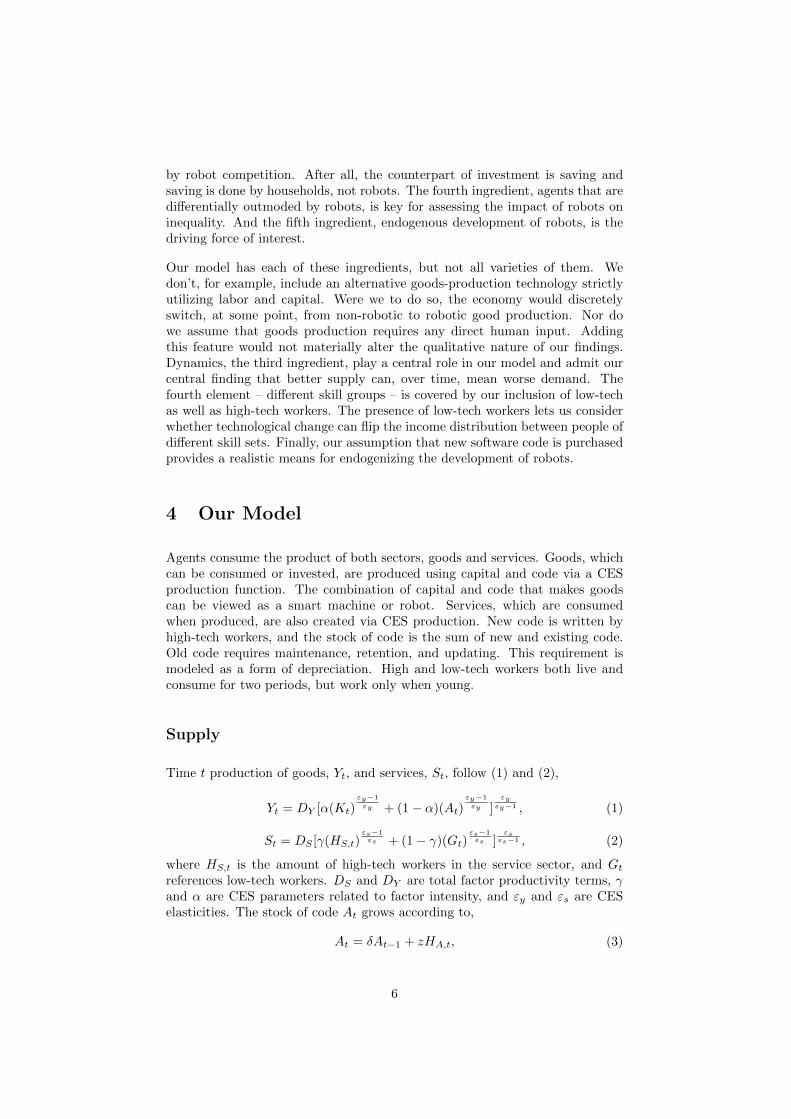
Time t production of goods, Yt, and services, St, follow (1) and (2),

Yt = DY [α(Kt)εy−1

εy + (1− α)(At)εy−1

εy ]εy

εy−1 , (1)

St = DS [γ(HS,t)εs−1εs + (1− γ)(Gt)

εs−1εs ]

εsεs−1 , (2)

where HS,t is the amount of high-tech workers in the service sector, and Gt

references low-tech workers. DS and DY are total factor productivity terms, γand α are CES parameters related to factor intensity, and εy and εs are CESelasticities. The stock of code At grows according to,

At = δAt−1 + zHA,t, (3)

6

where the “depreciation” factor is δ ∈ [0, 1). Higher δ means that legacy codeis useful longer. HA,t is the amount of high-tech labor hired by good firms, andz is the productivity of high-tech workers writing code.

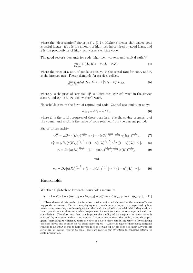
The good sector’s demands for code, high-tech workers, and capital satisfy3

maxKt,At

Yt(At,Kt)−mtAt − rtKt, (4)

where the price of a unit of goods is one, mt is the rental rate for code, and rtis the interest rate. Factor demands for services reflect,

maxHS,t,Gt

qtSt(HS,t, Gt)− wGt Gt − wH

t HS,t, (5)

where qt is the price of services, wHt is a high-tech worker’s wage in the service

sector, and wGt is a low-tech worker’s wage.

Households save in the form of capital and code. Capital accumulation obeys

Kt+1 = φIt − ptδAt, (6)

where It is the total resources of those born in t, φ is the saving propensity ofthe young, and ptδAt is the value of code retained from the current period.

Factor prices satisfy

wHt = qtDS [γ(HS,t)

εs−1εs + (1− γ)(Gt)

εs−1εs ]

1εs−1 [γ(HS,t)

− 1εs ], (7)

wGt = qtDS [γ(HS,t)

εs−1εs + (1− γ)(Gt)

εs−1εs ]

1εs−1 [(1− γ)(Gt)

− 1εs ], (8)

rt = DY [α(Kt)εy−1

εy + (1− α)(At)εy−1

εy ]1

εy−1 [α(Kt)− 1

εy ], (9)

and

mt = DY [α(Kt)εy−1

εy + (1− α)(At)εy−1

εy ]1

εy−1 [(1− α)(At)− 1

εy ]. (10)

Households

Whether high-tech or low-tech, households maximize

u = (1− φ)[(1− κ)logcy,t + κlogsy,t] + φ[(1− κ)logco,t+1 + κlogso,t+1], (11)

3To understand this production function consider a firm which provides the service of ’mak-ing good chess moves’. Better chess playing smart machines are, in part, distinguished by howmany game trees they can investigate and the level of sophistication with which they evaluateboard positions and determine which sequences of moves to spend more computational timeconsidering. Therefore, our firm can improve the quality of its output (the chess move itchooses) by increasing either of its inputs. It can either increase the quality of its chess pro-gram (increasing its efficiency units of code) or devote more computing time to investigatingpossible moves and counter-moves (rent more capital). While the logic of decreasing marginalreturns to an input seems to hold for production of this type, this does not imply any specificstructure on overall returns to scale. Here we restrict our attention to constant returns toscale production.

7

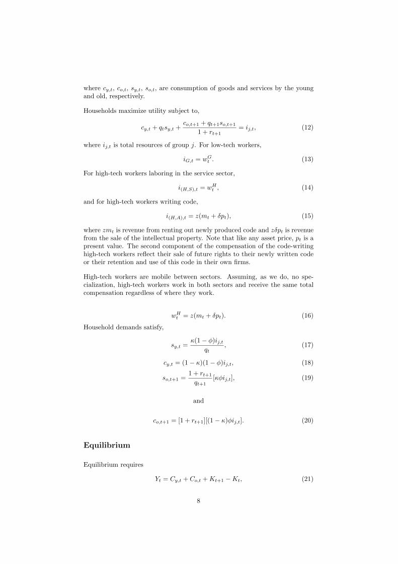
where cy,t, co,t, sy,t, so,t, are consumption of goods and services by the youngand old, respectively.

Households maximize utility subject to,

cy,t + qtsy,t +co,t+1 + qt+1so,t+1

1 + rt+1= ij,t, (12)

where ij,t is total resources of group j. For low-tech workers,

iG,t = wGt . (13)

For high-tech workers laboring in the service sector,

i(H,S),t = wHt , (14)

and for high-tech workers writing code,

i(H,A),t = z(mt + δpt), (15)

where zmt is revenue from renting out newly produced code and zδpt is revenuefrom the sale of the intellectual property. Note that like any asset price, pt is apresent value. The second component of the compensation of the code-writinghigh-tech workers reflect their sale of future rights to their newly written codeor their retention and use of this code in their own firms.

High-tech workers are mobile between sectors. Assuming, as we do, no spe-cialization, high-tech workers work in both sectors and receive the same totalcompensation regardless of where they work.

wHt = z(mt + δpt). (16)

Household demands satisfy,

sy,t =κ(1− φ)ij,t

qt, (17)

cy,t = (1− κ)(1− φ)ij,t, (18)

so,t+1 =1 + rt+1

qt+1[κφij,t], (19)

and

co,t+1 = [1 + rt+1][(1− κ)φij,t]. (20)

Equilibrium

Equilibrium requires

Yt = Cy,t + Co,t +Kt+1 −Kt, (21)

8

and

St = Sy,t + So,t, (22)

where Cy, Co, Sy, So, are total consumption demand of goods and services bythe young and old respectively.

Asset-market clearing entails equal investment returns on capital and code, i.e.,

pt =

∞∑s=t

R−1s+1,tδs+1−tms+1, (23)

where Rs,t is the compound interest factor between t and s, i.e.,

Rs,t =

s∏j=t

(1 + rj). (24)

Solving the Model

We calculate the economy’s perfect foresight transition path following an im-mediate and permanent increase in the rate of code retention due, for example,to the development of the silicon chip. The solution is via Gauss-Seidel iter-ation (see Auerbach and Kotlikoff, 1987). First, we calculate the economy’sinitial and final steady states. This yields initial and final stocks of capitaland code. These steady-state values provide, based on linear interpolation, ourinitial guesses for the time paths of the two input stocks. Next, we calculateassociated guesses of the time paths of factor prices as well as the price paths ofcode and services. Step three uses these price paths and the model’s demand,asset arbitrage, and labor market conditions to derive new paths of the suppliesof capital and code. The new paths are weighted with the old paths to formthe iteration’s next guesses of capital and code paths. The convergence of thisiteration, which occurs to a high degree of precision, implies market clearing ineach period.

5 Simulating Transition Paths

The models’ main novelty is the inclusion of the stock of code in the productionof goods. When the code retention rate, δ equals zero, good sector productionis conventional – based on contemporaneous amounts of capital and labor (codewriters). But when δ rises, good production depends not just on capital andcurrent labor, but, implicitly, on dead high-tech workers as well. We study theeffects of this technological change by simulating an immediate and permanentincrease in δ.

The increase in δ initially raises the compensation of code-writing high-techworkers. This draws more high-tech workers into code-writing, thereby raising

9

high-tech worker compensation in both sectors. In most parameterizations, theconcomitant reduction in service output raises the price of services. And, de-pending on the degree to which high-tech workers compliment low-tech workersin producing services, the wages of low-tech workers will rise or fall.

Things change over time. As more durable code comes on line, the marginalproductivity of code falls, making new code writers increasingly redundant.Eventually the demand for code-writing high-tech workers is limited to thoseneeded to cover the depreciation of legacy code, i.e., to retain, maintain, andupdate legacy code. The remaining high-tech workers find themselves working inthe service sector. The upshot is that high-tech workers can end up potentiallyearning far less than in the initial steady state.

What about low-tech workers?

The price of services peaks and then declines thanks to the return of high-techworkers to the sector. This puts downward pressure on low-tech workers’ wagesand, depending on the complementarity of the two inputs in producing services,low-tech workers may also see their wages fall. In this case, the boom-bust inhigh-tech workers’ compensation generates a boom-bust in low-tech compensa-tion. In the extreme, if high and low-tech workers are perfect substitutes, theirwages move in lock step.

The economy’s dynamic reaction to the higher δ depends on the impact on cap-ital formation. The initial rise in earnings of at least the high-tech workers canengender more aggregate saving and investment. The increased capital makescode and, thus, high-tech workers more productive. But if the compensation ofhigh-tech and, potentially, low-tech workers falls, so too will the saving of theyoung and the economy’s supply of capital. Less capital means lower marginalproductivity of code and higher interest rates. This puts additional downwardpressure on new code rental rates as well as on the price of future rights to theuse of code.

We next consider four possible transition paths, labeled Immiserizing Growth,Felicitous Growth, The First Will be Last, and Better Tasting Goods. Eachsimulation features an immediate and permanent rise in the code-retention rate.But the dynamic impact of this technological breakthrough can be good for someand bad for others depending on the size of the shock and other parameters.After presenting these cases, we examine the sensitivity of long-run outcomesto parameter assumptions more systematically.

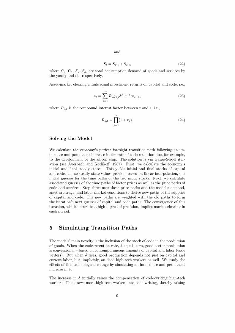
Immiserating Growth

Figure 1 shows that a positive tech shock (the code-preservation rate, δ, risesfrom 0 to .7) can have very negative long-term consequences. The simulationassumes Cobb-Douglas production of goods and linear production of services;i.e., both types of workers are perfect substitutes in producing services (εS =∞).

10

As the top left panel indicates, national income quickly rises – by 13 percent.But it ultimately declines, ending up 28 percent below its initial steady-statevalue. Since preferences are logarithmic, expenditures on goods and serviceschange by the same percentage. In the case of services, however, this occurs notonly through changes in output levels, but also via changes in relative price.

The relative price of services first rises and then falls dramatically, while serviceoutput does the opposite. Good output moves pari passus with national income.Hence, in the long-run, both young and old agents end up consuming 28 percentless goods. And while their consumption of services is 27 percent larger, it’s notworth very much at the margin. In fact, its price is 43 percent lower than beforethe technological breakthrough.

Both types of worker earn the same under this parameterization. Their com-pensation initially jumps 16 percent and then starts to fall dramatically. In thelong run all workers end up earning 44 percent less than was originally the case!

What happens to the welfare of different agents through time? The initial elderlyare essentially unaffected by the tech boom. The initial young experience a 14percent rise in lifetime utility, measured as a compensating differential relativeto their initial steady-state utility. But those born in the long run are 17 percentworse off.

The top right chart helps explain why good times presage bad times. The stockof code shoots up and stays high. But the stock of capital immediately startsfalling. After six periods there is over 50 percent more code, but 65 percent lesscapital.

The huge long-run decline in the capital stock and associated rise in its marginalproduct (the interest rate) has two causes. First, as just stated, wages, whichfinance the acquisition of capital, are almost cut in half by the implicit compe-tition with dead workers. Second, the advent of a new asset – durable code –crowds out asset accumulation in the form of capital. When δ rises, all workersimmediately enjoy an increase in their compensation. This leads to more saving,but not more saving in the form of capital. Instead, their extra saving as wellas some of the saving they originally intended to do is used to acquire claimsto legacy code. Initially, when the stock of code is small, its price is high. And,later, when the stock of code is large, its price is low – some 56 percent below itsinitial value. However, the total value of code increases enough to significantlycrowd out investment in capital along the entire transition path.

Another way to understand capital’s crowding out is to view legacy code, whichcoders can sell or retain when the code retention rate rises, as a form of futurelabor income. This higher resource permits more consumption of goods by low-tech workers (and high-tech workers, since they are paid the same) when theshock hits. And this additional good consumption means less goods are savedand invested. But the knock-on effect of having less capital in the economyis lower labor compensation. This reduces the consumption through time ofworkers, but also their saving.

What happens to labor’s share of national income? Initially it rises slightly.

11

But, in the long run, labor’s share falls from 75 to 57 percent. This reflects thehigher share of output paid to legacy code. The long-run decline in labor’s shareof national income arises in all our simulations except those in which preferencesshift toward the consumption of goods at the same time as the code retentionrate rises.

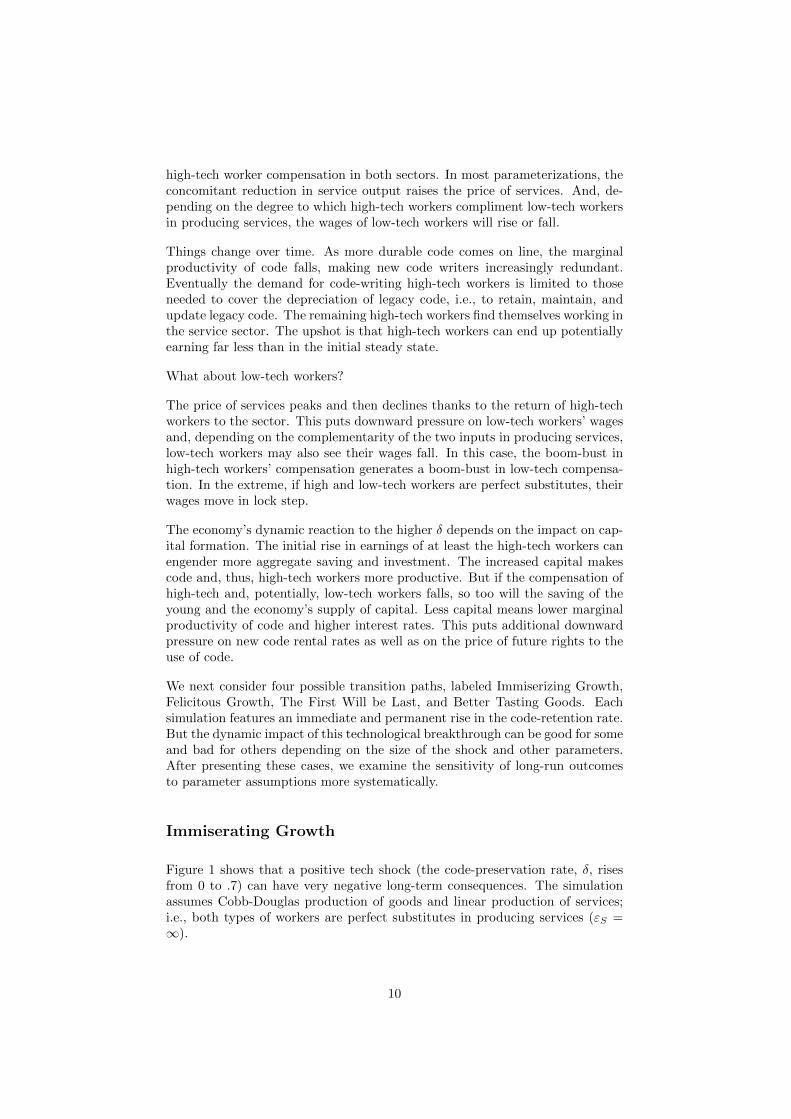
Felicitous Growth

As figure 2 shows, the tech boom need not auger long-term misery. A highersaving rate is the key. In the immiserating growth case above, we assumed asaving rate, φ, of .2. This generated a ratio of consumption when young toconsumption when old of 1.5 in the initial steady state and .9 in the long runsteady state. Here we assume a saving rate of .95 while holding fixed the model’sother parameter values. The result is that good times can be good for good.But the road is rocky. Output ends up permanently higher, but only after anintervening depression. Output of both goods peaks in the period after theshock, with national income rising 52 percent. But in the long-run, it is only20 percent higher – a major decline from its peak. The long-run expansion inoutput reflects less capital decumulation. In the prior simulation the capitalstock immediately declined. Here the capital stock temporarily increases 14percent above its initial value.

A less rapid decline in the capital stock and higher service prices boosts thecommon wage in the short term and leaves it above its initial value in the longrun. After peaking 50 percent above its initial value, the wage falls, endingup only 2 percent higher. The stock of code ends up more than twice as high.But the capital stock, notwithstanding the high rate of saving, declines by 35percent.

The respective increase and decrease in the stocks of code and capital producea significant rise in the economy’s interest rate – 74 percent in the long run.Although the labor compensation of high and low-tech workers ends up veryclose to where it started, this increase in the interest rate permits those livingin the future to consume 20 percent more.

Why does a high enough saving rate keep the δ shock from reducing long-run welfare? The answer is that whatever happens to the stock of code, ahigher saving rate entails a higher capital stock and, therefore, higher laborcompensation payments to high-tech workers. In the two above examples, we’veconsidered widely varying saving rates. If, instead, we consider an intermediatevalue of φ = .5, long-run national income still decreases, but by less – only10 percent compared with its initial steady state value. Figure 7 shows howlong-run output varies with φ and δ.

12

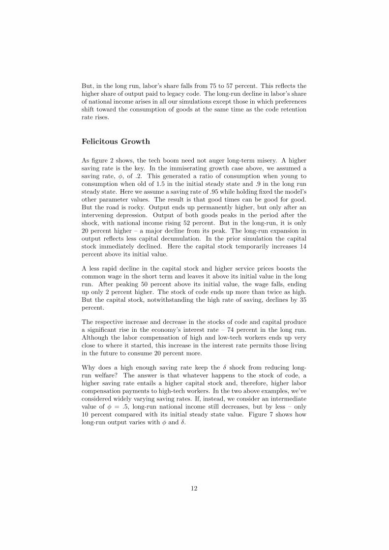
The First Will Be Last

If high and low-tech workers are compliments in producing services, their wageand utility paths will diverge. Consider, for example, the model with table2’s parameters shown in figure 3. As is always the case, the initial effect forhigh-tech worker of the δ shock is positive. Indeed, immediately after the shockhits, high-tech workers make 43 percent more than in the previous period. Butlow-tech workers, who, in this case, need high-tech workers to be productive,see their wages rise only 10 percent as the share of high-tech workers workingin services immediately falls from 50 percent to 38 percent.

However, as code accumulates and capital decumulates, high-tech workers startearning less in code-writing and move in great number back to the service sector.Ultimately, 68 percent of high-tech workers work in the service sector. And theirreturn to that sector drives down their wage compared both its initial value andto the long-run wage of low-tech workers. Indeed, in the final steady state,high-tech workers earn 14 percent less than in the initial steady state. Low-techworkers, in contrast, earn 17 percent more. But, interestingly, in period 3 theirwage peaks 41 percent above its original value. This rise and fall in the wagesof low-tech workers reflects, in part, the rise and fall in the price of services.

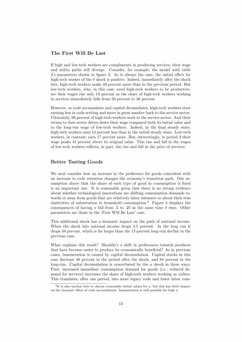
Better Tasting Goods

We next consider how an increase in the preference for goods coincident withan increase in code retention changes the economy’s transition path. Our as-sumption above that the share of each type of good in consumption is fixedis an important one. It is reasonable given that there is no strong evidenceabout whether technological innovations are shifting consumption demands to-wards or away from goods that are relatively labor intensive or about their trueelasticities of substitution in household consumption.4 Figure 4 displays theconsequences of having κ fall from .5 to .25 at the same time δ rises. Otherparameters are those in the ‘First Will Be Last’ case.

This additional shock has a dramatic impact on the path of national income.When the shock hits national income drops 2.5 percent. In the long run itdrops 48 percent, which is far larger than the 17-percent long-run decline in theprevious case.

What explains this result? Shouldn’t a shift in preferences towards productsthat have become easier to produce be economically beneficial? As in previouscases, immiseration is caused by capital decumulation. Capital stocks in thiscase decrease 40 percent in the period after the shock, and 84 percent in thelong-run. Capital decumulation is exacerbated by the κ shock in three ways.First, increased immediate consumption demand for goods (i.e., reduced de-mand for services) increases the share of high-tech workers working as coders.This translates, after one period, into more legacy code and lower labor com-

4It is also unclear how to choose reasonable initial values for κ, but this has little impacton the dynamic effect of code accumulation. Immiseration is still possible for high κ.

13

pensation, the source of saving and capital formation. Second, the increase inimmediate good consumption reduces the amount of capital available to invest.Third, the shift in demand toward goods limits the rise in the price of services.This, too, has a negative impact on wages and capital formation. Figure 8shows the sensitivity of the model to κ shocks of different sizes. Even withouta δ shock, a shift in preferences towards goods is bad for long-run outcomes.

The Large Range of Potential Outcomes

As just demonstrated, the model’s reaction to the δ shock is highly sensitiveto parameter values. We now consider this sensitivity in more detail. Figure5 jointly displays our previous results. Table 3 shows additional results forseveral different parameter combinations. The table’s baseline simulation (rowone) assumes intermediate parameter values. Subsequent rows show the impactof sequentially modifying one parameter. Figure 6 plots the path of nationalincome for each row of the table.

These simulations teach several new things. First, high-tech workers benefitfrom substitutability in the goods sector. In the perfect substitutability casethe productivity of high-tech workers is independent of supplies of code andcapital.

Second, as one can show analytically, with both Cobb-Douglas production andpreferences, the path of the capital-to-code ratio is independent of the rela-tive supplies of the two typtes of workers. Since the compensation of high-techworkers is pegged to the capital-to-code ratio, reducing the number of high-techworkers, holding fixed the number of low-tech workers, leaves the compensa-tion of high-tech workers unchanged. In contrast, holding fixed the number ofhigh-tech workers and reducing the number of low-tech workers raises the com-pensation of low-tech workers. In the former case of fewer high-tech workers,the number of coders is fully supplemented by movement of high-tech work-ers from services into coding. In the latter case of fewer low-tech workers, thenumber of high-tech workers coding and working in the service sector stays thesame along the transition path. Furthermore, high-tech workers earn the samein services because the rise in the price of services exactly offsets their lowermarginal productivity resulting from having fewer low-tech workers with whomto work.5

Third, a positive δ shock always produces a tech boom with increases in boththe price of code and the wage of high-tech workers.6 In most simulations, the

5To get some intuition for these results, consider the case that the δ shock arises in thecontext of a smaller number of low-tech workers. If the price of services rises by the samepercentage that the number of low-tech workers falls, there will be no change in the valueof service output, measured in goods. Nor will there be any change in the other componentof national income – good output. Since national saving is a fixed share of national income(given the Cobb-Douglas preferences), the path of the capital stock as well as the path ofthe code stock will not change from what would otherwise have been the case. So high-techworkers, whose numbers are unchanged, earn the same amount in total and per person. Incontrast, low-tech workers experience a rise in their wages.

6This can be shown analytically.

14

boom is short lived, auguring a major tech and saving bust. Fourth, in mostsimulations capital becomes relatively scarce compared to code leading to a risein interest rates. Finally, the δ shock generally raises labor share in the shortrun and lowers it in the long run.

Figure 7 presents a contour graph of long-run national income. Its top halfconsiders combinations of shocks to δ and the saving rate φ assuming table 1’svalues of the other parameters. Redder areas denote higher long-run nationalincome relative to the initial steady state. Bluer areas denote the opposite.Long-run national income increases most when δ is large and the saving rate ishigh. It decreases the most when the δ shock is high and the saving rate is low.

Figure 7’s bottom half considers joint shocks to the saving rate and code-writingproductivity (z). Higher values of each reinforces their individual positive im-pacts on long-run national income. As opposed to δ shocks, shocks to code-writing productivity (z) enhance all agents’ welfare. The reason is simple – thisshock makes living, but not dead high-tech workers more productive.

The top half of figure 8 examines joint shocks to δ and κ – services’ preferenceshare. As discussed in the Better Tasting Goods case, δ shocks do more long-run damage when they are accompanied by a rise in the preference for goods.This is not surprising. In the short run, higher good demand elicits more codeproduction, which eventuates in a larger long-run stock of code. Yes, there is alarger long-run demand for coders to maintain and retain the larger code stock.But this permanently larger code stock entails perpetually greater competitionof new high-tech workers with dead high-tech workers and means permanentlylower incomes to high-tech workers as well as low-tech workers. Stated differ-ently, if human automation is accompanied by increased demand for goods thatcan be automated, the long-run economic fallout is worse and, potentially, farworse than would arise were non-automatable goods to become relatively moredesirable.

The bottom panel in figure 8 considers combinations of the saving rate, φ, andthe good sector’s elasticity of substitution, εy. It shows the aforementionedsensitivity of long-run output to the substitutability of code for capital. Italso indicates that this sensitivity is greater for low than for high saving rates.Higher substitutability moderates the negative effects of capital’s crowding outthat occurs with low savings.

6 The Role of Property Rights and Rivalry

To this point we’ve assumed that code is private and rival. Specifically, we’veassumed that when one firm uses code it is unavailable for rent or use byother firms. But unlike capital, code represents stored information that maybe non-rival in its use. Non-rivalry does not however necessarily imply non-excludability. Patents, copyrights, trade secrets, and other means can be usedto limit code’s unlicensed distribution. On the other hand, the government canturn code into a public good by mandating it be open source.

15

This section explores two new scenarios. The first is that code is non rival andnon excludable in its use, i.e., it is a public good. The second is that code is nonrival, but excludable. To accommodate these possibilities we modify our modelin two ways. We assume that each firm faces a fixed cost of entry. And weassume that each firm is endowed with a limited supply of public code. Theseassumptions ensure a finite number of firms operating with non-trivial quantitiesof capital. To compare these two new settings with what came above – the caseof private (rival and excludable) code, we rewrite our baseline model with thetwo new assumptions.

Rival, Excludable (Private) Code

With a fixed public code endowment and fixed entry costs, profit maximizationsatisfies:

πj,t = F (kj,t, zHj,t + aj,t +A)− C − rtkj,t −mtaj,t, (25)

where πj,t are profits for firm j at time t, F (•) is the same CES productionfunction as in the baseline model, kj,t is the amount of capital rented by thefirm, aj,t is the amount of code rented by the firm, Hj,t is the amount of high-tech labor hired by the firm, A is the exogenously set amount of free code inthe economy, and C is the cost of creating a new firm. This cost must be paideach period. In equilibrium all firms have zero profits.

0 = F (kj,t, zHj,t + aj,t +A)− C − rtkt −mtaj,t. (26)

Market clearing conditions are,∑aj,t = δAt−1, (27)∑kj,t = Kt, (28)∑Hj,t = HA,t, (29)

Y = co,t + cy,t −Kt +Kt+1 +NC, (30)

where N is the number of firms. Since all firms are identical, (26) provides anexpression for N, the number of firms.

0 = NF (Kt

N, zHt +

1

NδAt−1 +A)−NC − rtKt −mtδAt−1 (31)

Firms enter up to the point that the value of the public code they obtain forfree, namely A, equals their fixed cost of production. Thus,

AFa,t = C. (32)

This fixes the marginal product of code at CA

in every period. Intuitively, newfirms can acquire a perfect substitute for new code, and, thus, new coders at afixed cost by setting up shop and gaining access to A in free code. Given thatgood production obeys constant returns to scale, fixing code’s marginal product

16

means fixing the ratio of capital to code. This, in turn, fixes the interest rate.Hence, the rental rates of coders and capital are invariant to the increase in δ.

Although the increase in δ doesn’t raise the current productivity of coders, itdoes raise the present value of their labor compensation. The reason is thatcoders can now sell property rights to the future use of their invention. Hence,unlike our initial model, this variant with fixed costs and a free endowment ofcode does not admit immiserating growth absent some additional assumptions.7

Were the number of firms to remain fixed, the jump in δ would entail more codeper firm with no higher capital per firm. This would mean a lower marginalproductivity of code, which (32) precludes. It would also mean a negative payoffto setting up a new firm. Hence, the number of firms must shrink in order toraise the level of capital per firm as needed to satisfy (32).

To solve the model an additional step is added to the iteration procedure. Givena guess of prices and stocks in a period, (31) is used to calculate N . This guessof N in each period is included in the next iteration to calculate new prices.8

Figure 9 shows transition paths for key variables for this excludable, non-rivalmodel based on Table 4’s parameter values. Note that high-tech workers earn 14percent more in the long run and enjoy commensurately higher utility. Low-techworkers are also better off. There is also a modest increase in the economy’scapital stock.

Non-Rival, Non-Excludable (Public) Code

Consider next the case that code, in the period after it is produced, is a purepublic good used simultaneously by every firm. This possibility could arise bygovernment edict, the wholesale pirating of code, or reverse engineering.

Profits are now

πj,t = F (kj,t, zHj,t + aj,t +A)− C − rtkj,t, (33)

as firms no longer need to rent their stock of code (aj,t), where

aj,t = δAt−1∀j (34)

As before, firm entry and exit imply zero profits,

0 = NF (Kt

N, zHt + δAt−1 +A)−NC − rtKt. (35)

andδAt−1 +AFa,t = C. (36)

7If the number of firms is fixed due to oligopilization of the industry, equation (32) wouldnot hold, in which case the marginal productivity of code would again decrease as it accumu-lates.

8In what follows, we consider only equilibria in which high-tech workers work in bothsectors. If the public endowment is large enough in a period, goods firms will require no newcode.

17

Finally, with investment in code no longer crowding out investment in capital,

Kt+1 = φIt. (37)

Figure 10 shows results for this case again with Table 4’s parameter values.The initial steady state is the same as in the prior case of excludable rival code.However, the response to the jump in δ are dramatically different. The jump inδ has no immediate impact on the economy because high-tech workers no longerhold copyright to their code.

In the period after the shock, the economy begins to react. The stock of freepublic code, which now includes both A plus all of the economy’s legacy code,is larger. This induces more firm entry. Indeed, the number of firms morethan doubles. As indicated in equation (36), with more free code available, newentrants can cover the fixed costs of entry with a lower value per unit of freecode, i.e., with a lower marginal product of code. The lower marginal productof code and, thus, of coders leads to an exodus of high-tech workers from codinginto services. In the long run, the number of high-tech workers hired for theircoding skills falls by 30 percent and their wage falls by 25 percent. Nationalincome peaks at 5 percent above its initial level in this period. The interest raterises by 35 percent and the wage of low-tech workers decreases by 10 percent.

The economy’s transition is characterized by a series of damped oscillations asperiods of relatively high coder hiring is followed by periods of plentiful freecode and relatively low coder hiring. Most importantly, the long-run impact ofthis change is a net immiseration with long-run national income 8 percent belowits initial steady state level.

As in the baseline model, the main mechanism for immiseration is the reductionof the high-tech wage leading to lower capital accumulation. A secondary reasonis the inefficiency introduced due to high-tech workers no longer being able tointernalize the full value of their creation of new code.

Non-Rival, Excludable (Private) Code

A third possibility is that code is excludable, but non-rival in its use, permittinghigh-tech workers to license all their code to all firms. The equations for therival, excludable model hold with the following exceptions. First, profits aregiven by

πj,t = F (kj,t, zHj,t + δAt−1 +A)− C − rtkj,t −mtδAt−1 (38)

Second, the price of code reflects its use by all firms.

pt =

∞∑s=t

R−1s+1,tδs+1−tms+1Ns+1. (39)

As shown in figure 11, the δ shock produces a felicitous transition path, indeedfar better than the rival excludable case. As in the rival, excludable case, firmsentry satisfies equation (32). Hence, the marginal product of new code is fixed.So is the marginal product of capital, i.e., the interest rate.

18

7 Endogenous Production Technology

So far we’ve assumed a single means of producing goods. Here we permit goodproducers to switch between more and less code-intensive production techniques.To keep matters simple we assume the good sector’s production function isCobb-Douglas and that good producers can choose the parameter on A (andthus on K) such that α ∈ [α1, α2]. In the initial steady state, α1 = α2, butwhen δ is shocked, the range of possible technologies is expanded as well.

This is simulated via an additional step in the iteration process. After a guess ofthe path of code and capital is made, an α ∈ [α1, α2] is selected in every periodto maximize good output. Subsequently, prices are calculated from marginalproducts and a new guess of the path of inputs is made.

Given the inputs, and the prevailing stocks of code and capital, output is convexin α. Hence, firms will produce using either the lowest or highest value.9 Thisresults in the economy flipping back and forth repeatedly, although not nec-essarily every period, from the most to the least capital-intensive technology.Since our solution method relies on the economy reaching a stable steady state,we set α to a fixed value, namely α2, far enough in the future such that thetransition path for the initial several hundred periods is unaffected.

Figure 12 presents results based on table 5’s parameter values. Unlike theprevious figures, the absolute amounts of capital and code stocks reflect thedependency of the choice of technology on the ratio of the two stocks. In theinitial steady state, the code stock consists just of newly produced code and,naturally, is low. The economy is in a capital-intensive steady state. After theδ shock, code begins to accumulate. In the fourth period, sufficient code is ac-cumulated to lead producers to switch technologies toward more code-intensiveproduction. But the switch to code-intensive production raises wages and, thus,workers’ saving. Due to our assumed high saving rate (φ = .9), the increase insaving more than offsets the increase in the value of claims to code and the cap-ital stock increases. If the saving rate were lower, capital stocks would not rise,and the economy would remain permanently in a code-intensive equilibrium.In this case, however, the increase in saving is large enough to drive producersto adopt a capital-intensive technology in the next period. This leads to lowerwages, which, over time, means a lower capital-code ratio and a subsequentswitch back to code-intensive production.

This ongoing cycle has important welfare implications. High-tech workers whoare young when the code-intensive technology is used will earn a high wagewhen young and high interest rates when old. Those unfortunate enough to beyoung in a period when a high alpha is chosen will earn low wages while youngand low interest rates when old.

Because a period in our model corresponds to roughly 30 years, this cycle oftechnologically driven booms and busts bears a striking resemblance to the‘long-wave’ theories of early economists such as Schumpeter and Kondratieff.

9Y ′′(α) = B AK

α(log(A)− log(K))2 must always be positive for K and A greater than zero

19

While evidence for the existence of such cycles is limited (Mansfield 1983), thismodel’s long-wave cycles reflect a different mechanism from those in Rosenbergand Frischtak (1983).

8 Conclusion

Will smart machines, which are rapidly replacing workers in a wide range of jobs,produce economic misery or prosperity? Our two-period, OLG model admitsboth outcomes. But it does firmly predict three things - a long-run declinein labor share of income (which appears underway in OECD members), tech-booms followed by tech-busts, and a growing dependency of current output onpast software investment.

The obvious policy for producing a win-win from higher code retention is taxingthose workers who benefit from this technological breakthrough and saving theproceeds. This will keep the capital stock from falling and provide a fund topay workers a basic stipend as their wages decline through time. Other policiesfor managing the rise of smart machines may backfire. For example, restrictinglabor supply may reduce total labor income. While this may temporarily raisewages, it will also reduce investment and the long-term capital formation onwhich long-term wages strongly depend. Another example is mandating thatall code be open source. This policy removes one mechanism by which capitalis crowded out, but it leads firms to free ride on public code rather than hirenew coders. This reduces wages, saving, and, in time, the capital stock.

Our simple model illustrates the range of things that smart machines can do forus and to us. Its central message is disturbing. Absent appropriate fiscal policythat redistributes from winners to losers, smart machines can mean long-termmisery for all.

20

References

1. Acemoglu, D. 1998. Why do new technologies complement skills? Directedtechnical change and wage inequality. Quarterly Journal of Economics 113No. 4 (November): 1055-1089.

2. Acemoglu, D. & Autor, D. 2011. Skills, tasks and technologies: Impli-cations for employment and earnings. Handbook of Labor Economics 4:1043-1171.

3. Acemoglu, D., Autor, D. H., Dorn, D., Hanson, G. H., & Price, B. 2014.Return of the solow paradox? IT, productivity, and employment in U.S.manufacturing. American Economic Review American Economic Associ-ation 104 No. 5 (May): 394-399.

4. Arrow, K. A. 1962. The economic implications of learning by doing. TheReview of Economic Studies 29 No. 3 (June): 155-173

5. Autor, D. H., Levy, F., & Murnane, R. J. 2003. The skill content ofrecent technological change: An empirical exploration. Quarterly Journalof Economics 118 No.4 (Novemeber): 1279-1333.

6. Autor, D. H., & Dorn, D. 2013. The growth of low-skill service job andthe polarization of the US labor market. American Economic Review 103No. 5 (August): 1553-1597.

7. Brynjolfsson, E., & McAfee., A. 2011. Race Against the Machine. Lex-ington Digital Frontier Press.

8. Frey, C. B., & Osborne, M. A. 2013. The future of employment: howsusceptible are jobs to computerisation? Oxford University (September).

9. Goos, M., Manning, A., & Salomons, A. 2010. Explaining job polarizationin Europe: The roles of technology, globalization and institutions. Centrefor Economic Performance Discussion Papers. No. 1026. (November).

10. Hemous, D., & Olsen, M. 2013. The Rise of the Machines: Automation,Horizontal Innovation and Income Inequality. Horizontal Innovation andIncome Inequality

11. Katz, L. F., & Margo, R. A. 2013. Technical change and the relativedemand for skilled labor: The united states in historical perspective. Na-tional Bureau of Economic Research No. w18752.

12. Kelly, K. The Three Breakthroughs That Have Finally Unleashed AI onthe World.Wired Online Edition, October 27, 2014. Website:http://www.wired.com/2014/10/future-of-artificial-intelligence/

13. Keynes, J. M. 1933. Economic possibilities for our grandchildren 1930.Essays in persuasion. New York: W.W.Norton & Co., 1963, pp. 358-373.

14. Kotlikoff, L. J. & Sachs, J. D. 2012. Smart machines and long-term mis-ery.(Working Paper No. 18629). Retrieved from Nationl Bureau of Eco-nomic Research website: http://www.nber.org/papers/w18629

21

15. Kondratieff, N.D., & Stolper, W. F. 1935 The long waves in economic life.The Review of Economics and Statistics 17 No. 6 (November): 105-115.

16. Lucas, R. 1988. On the mechanics of economic development. Journal ofMonetary Economics 22 (February): 3-42.

17. Madrigal, A. Inside Google’s secret drone delivery program.The AtlanticOnline Edition, August 28, 2014. Website: http://www.theatlantic.com/technology/archive/2014/08/inside-googles-secret-drone-delivery-program/379306/

18. Mansfield, E. 1983. Long waves and technological innovation. The Amer-ican Economic Review 73 No. 2 (May): 141-145.

19. Marx, K. 1867. Capital: A Critique of Political Economy. Penguin Clas-sics Vol 1 (1992).

20. Mishel, L., Schmitt, J., & Shierholz, H. 2013. Don’t blame the robots.Assessing the job polarization explanation of growing wage inequality.CEPR Working Paper November 19, 2013. National Archives UnitedKingdom Government.

21. Luddites: The Growth of Political Rights in Britain in the 19th Cen-tury. Website of the National Archives. Retrieved January 20, 2015, fromhttp://www.nationalarchives.gov.uk/education/politics/g3/

22. May 2013 OES National Industry-Specific Occupational Employment andWage Estimates. (n.d.). Retrieved January 20, 2015, fromhttp://www.bls.gov/oes/current/oessrci.htm

23. Nelson, R. & Phelps, E. 1966. Investment in humans, technological diffu-sion, and economic growth. The American Economic Review, 56(1/2):pp.69–75

24. Romer, P. 1990. Endogenous Technological Change. Journal of PoliticalEconomy 98, no. 5 (September): 71-102

25. Rosenberg, N., & Frischtak, C. R. 1983. Long waves and economic growth:a critical appraisal. American Economic Review 73 No. 2 (May): 146-151.

26. Rourke, K. H., Rahman, A. S., & Taylor, A. M. 2013. Luddites, theindustrial revolution, and the demographic transition. The Journal ofEconomic Growth 18 No. 4 (December): 373-409.

27. Schumpeter, J. A. 1939. Business cycles (Vol. 1, pp. 161-74). New York:McGraw-Hill.

28. Zeira, J. 1998. Workers, Machines, and Economic Growth. The QuarterlyJournal of Economics 113 No. 4 (November): 1091-1117.

22

Table 1Parameters for Immiserating Growth

Model Parameter Role Value

εs Elasticity in Service Sector ∞εy Elasticity in Good Sector 1γ Service High-Tech Input Share Param. 0.5α Good Capital Input Share Param. 0.5δ Code Retention Rate 0 shocked to 0.7φ Saving Rate 0.2H High-Tech Worker Quantity 1G Low-Tech Worker Quantity 1κ Service Consumption Share 0.5z Code Writing Productivity 1Dy TFP in Goods 1Ds TFP in Services 1

Table 1: This table gives parameter values for the first illustration of the effects ofa one-time, permanent increase in the depreciation rate, δ, from zero to .7. We takethe intermediate value of .5 for κ, α, and γ. The productivity terms z, DY , and DS ,are set to one. σ takes its CD value of zero, ρ, the CES substitution parameter, takeson the perfect-substitute value of 1. φ is the saving rate. In this and all subsequentsimulations invoking an elasticity of 1 (except for the endogenous technology extension)the true elasticity is actually 1.0001

23

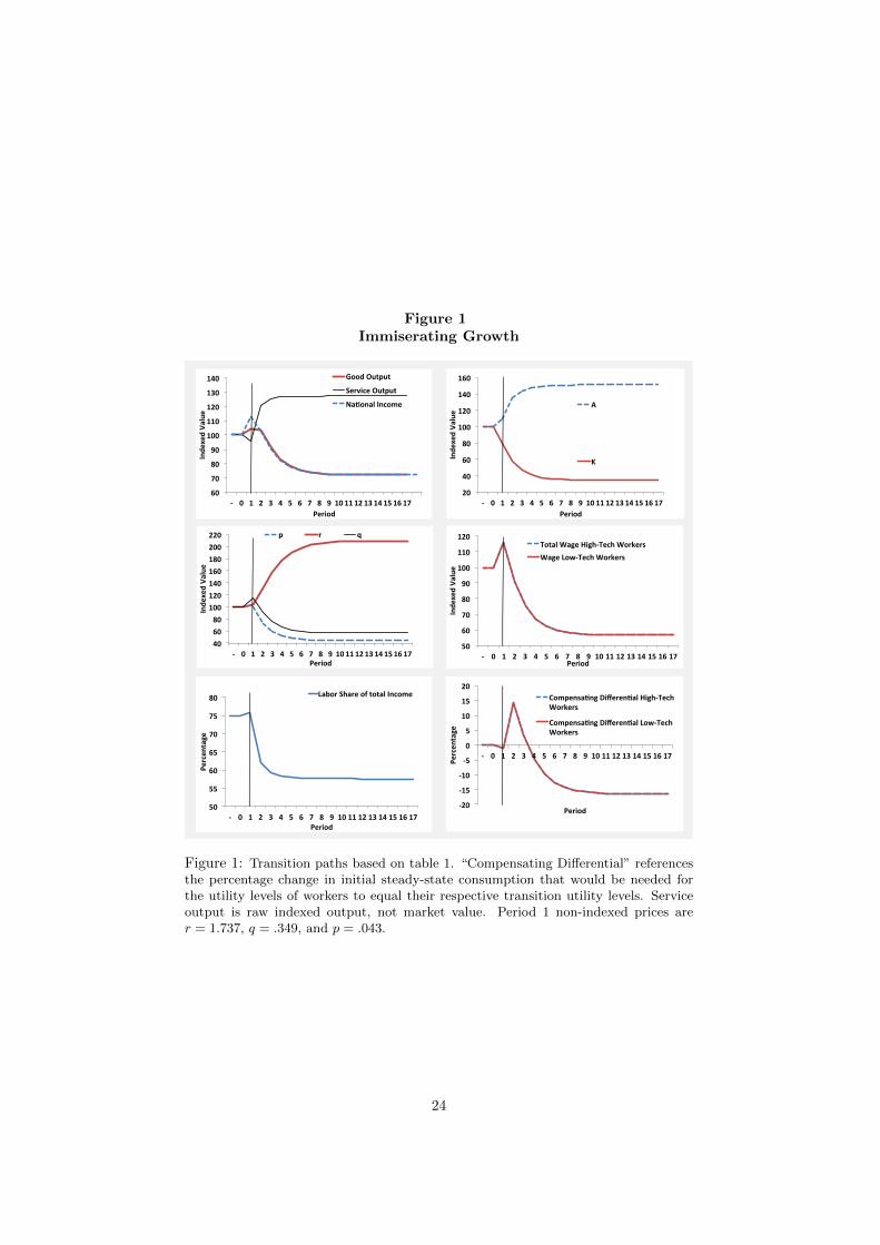
Figure 1Immiserating Growth

20#

40#

60#

80#

100#

120#

140#

160#

(# 0# 1# 2# 3# 4# 5# 6# 7# 8# 9# 10#11#12#13#14#15#16#17#

Inde

xed#Value

##

Period#

A#

K#

50#

60#

70#

80#

90#

100#

110#

120#

(# 0# 1# 2# 3# 4# 5# 6# 7# 8# 9# 10#11#12#13#14#15#16#17#

Inde

xed#Value

#

Period#

Total#Wage#High(Tech#Workers#

Wage#Low(Tech#Workers#

40#

60#

80#

100#

120#

140#

160#

180#

200#

220#

(# 0# 1# 2# 3# 4# 5# 6# 7# 8# 9# 10#11#12#13#14#15#16#17#

Inde

xed#Value

##

Period#

p# r# q#

50#

55#

60#

65#

70#

75#

80#

(# 0# 1# 2# 3# 4# 5# 6# 7# 8# 9# 10#11#12#13#14#15#16#17#

Percen

tage#

Period#

Labor#Share#of#total#Income#

60#

70#

80#

90#

100#

110#

120#

130#

140#

(# 0# 1# 2# 3# 4# 5# 6# 7# 8# 9# 10#11#12#13#14#15#16#17#

Inde

xed#Value

#

Period#

Good#Output#

Service#Output#

NaQonal#Income#

(20#

(15#

(10#

(5#

0#

5#

10#

15#

20#

(# 0# 1# 2# 3# 4# 5# 6# 7# 8# 9# 10#11#12#13#14#15#16#17#

Percen

tage#

Period#

CompensaQng#DifferenQal#High(Tech#Workers#

CompensaQng#DifferenQal#Low(Tech#Workers#

Figure 1: Transition paths based on table 1. “Compensating Differential” referencesthe percentage change in initial steady-state consumption that would be needed forthe utility levels of workers to equal their respective transition utility levels. Serviceoutput is raw indexed output, not market value. Period 1 non-indexed prices arer = 1.737, q = .349, and p = .043.

24

Figure 2Felicitous Growth

(higher saving rate, φ = .95)

60#

80#

100#

120#

140#

160#

180#

200#

220#

(# 0# 1# 2# 3# 4# 5# 6# 7# 8# 9# 10#11#12#13#14#15#16#17#

Inde

xed#Value

##

Period#

A#

K#

50#

70#

90#

110#

130#

150#

170#

(# 0# 1# 2# 3# 4# 5# 6# 7# 8# 9# 10#11#12#13#14#15#16#17#

Inde

xed#Value

##

Period#

Total#Wage#High(Tech#Workers#

Wage#Low(Tech#Workers#

60#

80#

100#

120#

140#

160#

180#

200#

(# 0# 1# 2# 3# 4# 5# 6# 7# 8# 9# 10#11#12#13#14#15#16#17#

Inde

xed#Value

##

Period#

p# r# q#

50#

55#

60#

65#

70#

75#

80#

(# 0# 1# 2# 3# 4# 5# 6# 7# 8# 9# 10#11#12#13#14#15#16#17#

Percen

tage#

Period#

Labor#Share#of#total#Income#

60#70#80#90#

100#110#120#130#140#150#160#

(# 0# 1# 2# 3# 4# 5# 6# 7# 8# 9# 10#11#12#13#14#15#16#17#

Inde

xed#Value

##

Period#

Good#Output#

Service#Output#

NaQonal#Income#

(15#(10#(5#0#5#

10#15#20#25#30#35#40#

(# 0# 1# 2# 3# 4# 5# 6# 7# 8# 9# 10#11#12#13#14#15#16#17#

Percen

tage#

Period#

CompensaQng#DifferenQal#High(Tech#Workers#

CompensaQng#DifferenQal#Low(Tech#Workers#

Figure 2: Transition paths based on table 1, with the exception of a higher savingrate (φ = .95). “Compensating Differential” references the percentage change in initialsteady-state consumption that would be needed for the utility levels of workers toequal their respective transition utility levels. Service output is raw indexed output,not market value. Period 1 non-indexed prices are r = .454, q = 2.204, and p = .631.

25

Figure 3The First Will Be Last

60#

80#

100#

120#

140#

160#

180#

200#

220#

240#

(# 0# 1# 2# 3# 4# 5# 6# 7# 8# 9# 10#11#12#13#14#15#16#17#

Inde

xed#Value

#

Period#

A#

K#

80#

90#

100#

110#

120#

130#

140#

150#

(# 0# 1# 2# 3# 4# 5# 6# 7# 8# 9# 10#11#12#13#14#15#16#17#

Inde

xed#Value

##

Period#

Total#Wage#High(Tech#Workers#

Wage#Low(Tech#Workers#

60#

80#

100#

120#

140#

160#

180#

200#

(# 0# 1# 2# 3# 4# 5# 6# 7# 8# 9# 10#11#12#13#14#15#16#17#

Inde

xed#Value

##

Period#

p# r# q#

50#

55#

60#

65#

70#

75#

80#

(# 0# 1# 2# 3# 4# 5# 6# 7# 8# 9# 10#11#12#13#14#15#16#17#

Percen

tage#

Period#

Labor#Share#of#total#Income#

80#

90#

100#

110#

120#

130#

140#

150#

(# 0# 1# 2# 3# 4# 5# 6# 7# 8# 9# 10#11#12#13#14#15#16#17#

Inde

xed#Value

#

Period#

Good#Output#

Service#Output#

NaQonal#Income#

(10#

0#

10#

20#

30#

40#

50#

(# 0# 1# 2# 3# 4# 5# 6# 7# 8# 9# 10#11#12#13#14#15#16#17#

Percen

tage#

Period#

CompensaQng#DifferenQal#High(Tech#Workers#

CompensaQng#DifferenQal#Low(Tech#Workers#

Figure 3: Transition paths based on table 2. “Compensating Differential” referencesthe percentage change in initial steady-state consumption that would be needed forthe utility levels of workers to equal their respective transition utility levels. Serviceoutput is raw indexed output, not market value. Period 1 non-indexed prices arer = .529, q = 1.317, and p = .398.

26

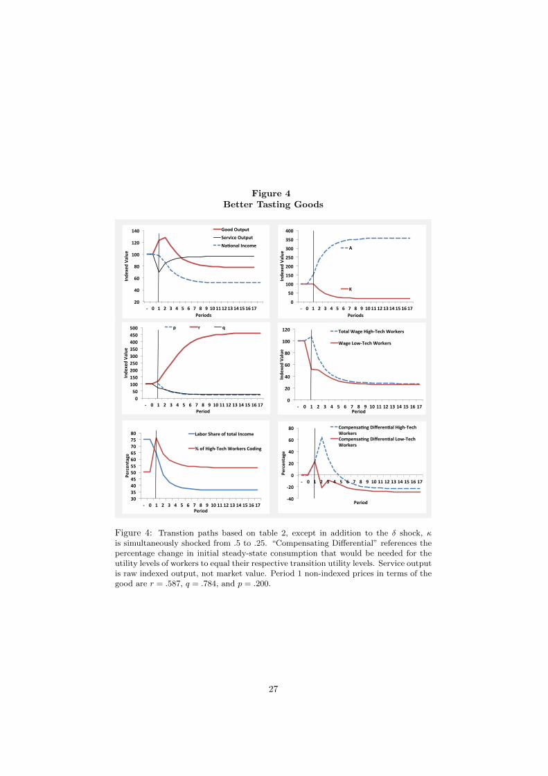
Figure 4Better Tasting Goods

0"

50"

100"

150"

200"

250"

300"

350"

400"

(" 0" 1" 2" 3" 4" 5" 6" 7" 8" 9" 10"11"12"13"14"15"16"17"

Inde

xed"Va

lue"

"

Periods"

A"

K"

0"

20"

40"

60"

80"

100"

120"

(" 0" 1" 2" 3" 4" 5" 6" 7" 8" 9" 10"11"12"13"14"15"16"17"

Inde

xed"Va

lue"

"

Period"

Total"Wage"High(Tech"Workers"

Wage"Low(Tech"Workers"

0"50"

100"150"200"250"300"350"400"450"500"

(" 0" 1" 2" 3" 4" 5" 6" 7" 8" 9" 10"11"12"13"14"15"16"17"

Inde

xed"Va

lue"

"

Period"

p" r" q"

30"35"40"45"50"55"60"65"70"75"80"

(" 0" 1" 2" 3" 4" 5" 6" 7" 8" 9" 10"11"12"13"14"15"16"17"

Percen

tage"

Period"

Labor"Share"of"total"Income"

%"of"High(Tech"Workers"Coding"

20"

40"

60"

80"

100"

120"

140"

(" 0" 1" 2" 3" 4" 5" 6" 7" 8" 9" 10"11"12"13"14"15"16"17"

Inde

xed"Va

lue"

"

Periods"

Good"Output"Service"Output"NaSonal"Income"

(40"

(20"

0"

20"

40"

60"

80"

(" 0" 1" 2" 3" 4" 5" 6" 7" 8" 9" 10"11"12"13"14"15"16"17"

Percen

tage"

Period"

CompensaSng"DifferenSal"High(Tech"Workers"CompensaSng"DifferenSal"Low(Tech"Workers"

Figure 4: Transtion paths based on table 2, except in addition to the δ shock, κis simultaneously shocked from .5 to .25. “Compensating Differential” references thepercentage change in initial steady-state consumption that would be needed for theutility levels of workers to equal their respective transition utility levels. Service outputis raw indexed output, not market value. Period 1 non-indexed prices in terms of thegood are r = .587, q = .784, and p = .200.

27

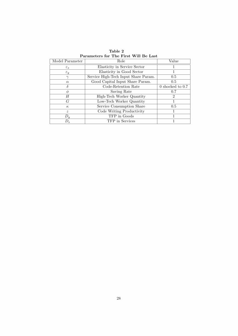
Table 2Parameters for The First Will Be Last

Model Parameter Role Value

εs Elasticity in Service Sector 1εy Elasticity in Good Sector 1γ Service High-Tech Input Share Param. 0.5α Good Capital Input Share Param. 0.5δ Code-Retention Rate 0 shocked to 0.7φ Saving Rate 0.7H High-Tech Worker Quantity 2G Low-Tech Worker Quantity 1κ Service Consumption Share 0.5z Code Writing Productivity 1Dy TFP in Goods 1Ds TFP in Services 1

28

Table

3:SensitivityAnalysis

Perio

dε s

ε yInitial.Steady.State

1.0

1.0

11.0

1.0

21.0

1.0

31.0

1.0

41.0

1.0

Baselin

e

δφ

Labo

r.High;

Tech.

Labo

r.Low

;Tech

κγ

z0.0

0.5

1.0

1.0

0.5

0.5

1.0

0.5

0.5

1.0

1.0

0.5

0.5

1.0

0.5

0.5

1.0

1.0

0.5

0.5

1.0

0.5

0.5

1.0

1.0

0.5

0.5

1.0

0.5

0.5

1.0

1.0

0.5

0.5

1.0

Baselin

e

Nat.IncomeGo

od.Outpu

tService.Outpu

tK

Ap

qr

Wage.High;

Tech.W

orkers

Wage.Low;

Tech.W

orkers

100

100.0

100.0

100.0

100.0

;100.0

100.0

50.0

100.0

121

117.5

106.4

100.0

112.6

100.0

116.3

106.1

54.4

124.4

118

116.0

109.1

96.6

143.0

89.6

116.2

121.7

61.9

109.2

114

113.2

109.6

88.3

152.4

83.6

110.6

131.4

60.3

101.3

112

111.0

109.7

82.1

156.0

80.0

106.0

137.8

58.1

96.7

Baselin

e

Labo

r.Share

%.High;Tech.

Workers.Cod

ing

Compe

nsating.

Diffe

rential.H

igh;

Tech.W

orkers

Compe

nsating.

Diffe

rential.Low

;Tech.W

orkers

75.0

50.0

0.0

;49.9

66.8

56.3

20.3

;47.4

65.6

43.4

8.9

;38.3

65.6

40.5

4.5

;37.7

64.8

39.9

2.3

;38.5

Baselin

e

101.0

1.0

0.5

0.5

1.0

1.0

0.5

0.5

1.0

107

107.0

109.6

71.9

159.8

74.2

98.0

149.1

53.7

89.5

62.7

40.0

;1.0

;40.5

Steady.State

1.0

1.0

0.5

0.5

1.0

1.0

0.5

0.5

1.0

107

106.7

109.5

71.1

160.0

73.8

97.4

150.0

53.4

88.9

62.5

40.0

;1.2

;40.7

Perio

dε s

ε yInitial.Steady.State

1.0

1.0

11.0

1.0

21.0

1.0

31.0

1.0

41.0

1.0

Service/Taste/Shock//κ

Jumps/from

/0.5/to

/0.75

δφ

Labo

r.High;

Tech.

Labo

r.Low

;Tech

κγ

z0.0

0.5

1.0

1.0

0.5

0.5

1.0

0.5

0.5

1.0

1.0

0.75

0.5

1.0

0.5

0.5

1.0

1.0

0.75

0.5

1.0

0.5

0.5

1.0

1.0

0.75

0.5

1.0

0.5

0.5

1.0

1.0

0.75

0.5

1.0Se

rvice/Taste/Shock//κ

Jumps/from

/0.5/to

/0.75

Nat.IncomeGo

od.Outpu

tService.Outpu

tK

Ap

qr

Wage.High;

Tech.W

orkers

Wage.Low;

Tech.W

orkers

100

100.0

100.0

100.0

100.0

;100.0

100.0

50.0

100.0

203

117.2

120.6

100.0

87.1

100.0

178.9

93.4

95.0

168.4

231

129.2

123.6

140.0

98.2

116.7

230.1

83.7

138.8

190.8

251

136.7

124.4

173.0

96.4

130.9

264.4

74.7

163.3

214.0

266

142.0

124.8

200.0

93.4

142.3

290.4

68.4

180.6

233.3

Service/Taste/Shock//κ

Jumps/from

/0.5/to

/0.75

Labo

r.Share

%.High;Tech.

Workers.Cod

ing

Compe

nsating.

Diffe

rential.H

igh;

Tech.W

orkers

Compe

nsating.

Diffe

rential.Low

;Tech.W

orkers

75.0

50.0

0.0

;49.8

58.4

43.6

20.3

;47.3

67.2

27.3

8.9

;38.2

72.0

23.7

4.5

;37.6

74.6

22.6

2.3

;38.4

Service/Taste/Shock//κ

Jumps/from

/0.5/to

/0.75

101.0

1.0

0.5

0.5

1.0

1.0

0.75

0.5

1.0

305

154.1

125.6

275.8

85.2

172.2

358.3

55.6

225.0

285.3

80.2

21.2

;1.0

;40.4

Steady.State

1.0

1.0

Perio

dε s

ε yInitial.Steady.State

1.0

1.0

11.0

1.0

21.0

1.0

31.0

1.0

41.0

1.0

Good

/Taste/Sho

ck//κ/Ju

mps/from

/0.5/to

/0.25

0.5

0.5

1.0

1.0

0.75

0.5

1.0

δφ

Labo

r.High;

Tech.

Labo

r.Low

;Tech

κγ

z0.0

0.5

1.0

1.0

0.5

0.5

1.0

0.5

0.5

1.0

1.0

0.25

0.5

1.0

0.5

0.5

1.0

1.0

0.25

0.5

1.0

0.5

0.5

1.0

1.0

0.25

0.5

1.0

0.5

0.5

1.0

1.0

0.25

0.5

1.0

Good

/Taste/Sho

ck//κ/Ju

mps/from

/0.5/to

/0.25

313

156.5

125.8

293.4

83.5

178.7

373.3

53.4

234.8

296.7

Nat.IncomeGo

od.Outpu

tService.Outpu

tK

Ap

qr

Wage.High;

Tech.W

orkers

Wage.Low;

Tech.W

orkers

100

100.0

100.0

100.0

100.0

;100.0

100.0

50.0

100.0

78117.2

81.6

100.0

149.3

100.0

69.2

122.2

24.6

97.1

67102.4

84.1

66.0

208.1

67.6

54.4

177.6

22.2

66.7

6091.9

84.8

44.9

233.3

52.4

43.7

227.9

18.4

51.9

5685.4

85.0

34.4

244.7

44.8

37.7

266.5

16.0

44.4

Good

/Taste/Sho

ck//κ/Ju

mps/from

/0.5/to

/0.25

81.3

20.9

;1.2

;40.6

Labo

r.Share

%.High;Tech.

Workers.Cod

ing

Compe

nsating.

Diffe

rential.H

igh;

Tech.W

orkers

Compe

nsating.

Diffe

rential.Low

;Tech.W

orkers

75.0

50.0

0.0

;49.9

70.5

74.7

22.3

;68.9

56.4

66.8

;4.5

;68.2

52.3

64.6

;18.2

;71.0

49.0

64.1

;25.7

;73.2

Good

/Taste/Sho

ck//κ/Ju

mps/from

/0.5/to

/0.25

101.0

1.0

0.5

0.5

1.0

1.0

0.25

0.5

1.0

5176.7

84.9

23.1

255.6

36.1

30.2

332.7

12.8

35.6

44.0

64.0

;34.9

;76.5

Steady.State

1.0

1.0

Perio

dε s

ε yInitial.Steady.State

1.0

1.0

11.0

1.0

21.0

1.0

31.0

1.0

41.0

1.0

Low/Saving/Ra

te φ/=/0.1

0.5

0.5

1.0

1.0

0.25

0.5

1.0

δφ

Labo

r.High;

Tech.

Labo

r.Low

;Tech

κγ

z0.0

0.1

1.0

1.0

0.5

0.5

1.0

0.5

0.1

1.0

1.0

0.5

0.5

1.0

0.5

0.1

1.0

1.0

0.5

0.5

1.0

0.5

0.1

1.0

1.0

0.5

0.5

1.0

0.5

0.1

1.0

1.0

0.5

0.5

1.0

Low/Saving/Ra

te φ/=/0.1

5176.3

84.9

22.7

255.9

35.7

30.0

335.6

12.7

35.3

Nat.IncomeGo

od.Outpu

tService.Outpu

tK

Ap

qr

Wage.High;

Tech.W

orkers

Wage.Low;

Tech.W

orkers

100

100.0

100.0

100.0

100.0

;100.0

100.0

49.9

100.0

100

100.8

110.5

100.0

102.3

100.0

105.6

101.2

52.2

106.8

9293.2

113.1

78.8

129.1

78.5

93.3

128.1

51.5

84.4

8888.1

113.8

63.7

136.6

68.6

83.4

146.6

47.2

73.8

8585.0

113.9

55.8

138.9

63.6

77.9

158.0

44.2

68.5

Low/Saving/Ra

te φ/=/0.1

43.8

64.0

;35.2

;76.6

Labo

r.Share

%.High;Tech.

Workers.Cod

ing

Compe

nsating.

Diffe

rential.H

igh;

Tech.W

orkers

Compe

nsating.

Diffe

rential.Low

;Tech.W

orkers

75.1

50.1

0.0

;50.0

77.5

51.2

6.8

;47.9

70.0

39.0

;9.3

;44.6

67.4

36.1

;15.9

;46.2

65.3

35.4

;19.0

;47.6

Low/Saving/Ra

te φ/=/0.1

101.0

1.0

0.5

0.1

1.0

1.0

0.5

0.5

1.0

8281.6

114.0

47.8

140.3

57.9

71.6

172.3

40.8

62.8

62.6

35.1

;22.3

;49.6

Steady.State

1.0

1.0

Perio

dε s

ε yInitial.Steady.State

1.0

1.0

11.0

1.0

21.0

1.0

31.0

1.0

41.0

1.0

51.0

1.0

High/Saving/Ra

te φ/=/0.9

0.5

0.1

1.0

1.0

0.5

0.5

1.0

δφ

Labo

r.High;

Tech.

Labo

r.Low

;Tech

κγ

z0.0

0.9

1.0

1.0

0.5

0.5

1.0

0.5

0.9

1.0

1.0

0.5

0.5

1.0

0.5

0.9

1.0

1.0

0.5

0.5

1.0

0.5

0.9

1.0

1.0

0.5

0.5

1.0

0.5

0.9

1.0

1.0

0.5

0.5

1.0

0.5

0.9

1.0

1.0

0.5

0.5

1.0

High/Saving/Ra

te φ/=/0.9

8181.4

114.0

46.9

140.4

57.9

71.5

172.6

40.7

62.6

Nat.IncomeGo

od.Outpu

tService.Outpu

tK

Ap

qr

Wage.High;

Tech.W

orkers

Wage.Low;

Tech.W

orkers

100

100.0

100.0

100.0

100.0

;100.0

100.0

50.0

100.0

131

126.9

103.2

100.0

121.5

100.0

117.7

110.2

52.2

132.9

132

129.4

106.3

104.4

154.4

95.0

126.1

121.6

65.1

122.3

130

128.9

107.0

102.0

164.1

92.1

125.2

126.8

66.6

117.7

129

128.0

107.2

99.2

167.5

90.3

123.2

129.9

66.0

115.1

128

127.3

107.1

97.1

168.9

89.1

121.5

131.9

65.1

113.4

High/Saving/Ra

te φ/=/0.9

62.5

35.1

;22.4

;49.6

Labo

r.Share

%.High;Tech.

Workers.Cod

ing

Compe

nsating.

Diffe

rential.H

igh;

Tech.W

orkers

Compe

nsating.

Diffe

rential.Low

;Tech.W

orkers

75.0

50.0

0.0

;49.9

60.9

60.8

25.0

;50.9

62.3

46.8

16.4

;38.0

63.7

43.5

13.7

;35.7

63.6

42.7

12.4

;35.5

63.4

42.6

11.7

;35.8

High/Saving/Ra

te φ/=/0.9

101.0

1.0

0.5

0.9

1.0

1.0

0.5

0.5

1.0

126

125.7

107.0

92.7

170.9

86.8

118.0

135.8

63.1

110.3

62.7

42.8

10.5

;36.7

Steady.State

1.0

1.0

0.5

0.9

1.0

1.0

0.5

0.5

1.0

125

125.4

106.9

91.8

171.3

86.3

117.2

136.5

62.7

109.6

62.5

42.8

10.3

;36.9

Inall

exam

ple

s,th

eδ

issh

ock

edfr

om

0in

the

init

ial

stea

dy

state

to.5

.Sim

ula

tions

subse

quen

tto

the

base

line

hav

eone

(hig

hlighte

d)

para

met

erch

anged

.E

ndogen

ous

vari

able

sare

index

ed.

Ser

vic

eoutp

ut

isin

mark

etva

lue

term

s.

29

Table

3Continued

Inall

exam

ple

sδ

issh

ock

edfr

om

0in

the

init

ial

stea

dy

state

to.5

.Sim

ula

tions

subse

quen

tto

the

base

line

hav

eone

(hig

hlighte

d)

para

met

erch

anged

.E

ndogen

ous

vari

able

sare

index

ed.

Ser

vic

eoutp

ut

isin

mark

etva

lue

term

s.

30

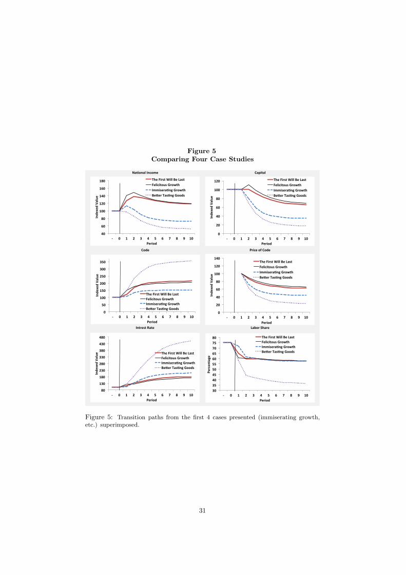
Figure 5Comparing Four Case Studies

National(Income Capital

Code Price(of(Code

Intrest(Rate Labor(Share

40(

60(

80(

100(

120(

140(

160(

180(

?( 0( 1( 2( 3( 4( 5( 6( 7( 8( 9( 10(

Inde

xed(Va

lue(

Period(

The(First(Will(Be(Last(Felicitous(Growth(ImmiseraMng(Growth(BeOer(TasMng(Goods(

0(

20(

40(

60(

80(

100(

120(

?( 0( 1( 2( 3( 4( 5( 6( 7( 8( 9( 10(

Inde

xed(Va

lue(

Period(

The(First(Will(Be(Last(Felicitous(Growth(ImmiseraMng(Growth(BeOer(TasMng(Goods(

0(

50(

100(

150(

200(

250(

300(

350(

?( 0( 1( 2( 3( 4( 5( 6( 7( 8( 9( 10(

Inde

xed(Va

lue(

Period(

The(First(Will(Be(Last(Felicitous(Growth(ImmiseraMng(Growth(BeOer(TasMng(Goods(

0(

20(

40(

60(

80(

100(

120(

140(

?( 0( 1( 2( 3( 4( 5( 6( 7( 8( 9( 10(

Inde

xed(Va

lue(

Period(

The(First(Will(Be(Last(Felicitous(Growth(ImmiseraMng(Growth(BeOer(TasMng(Goods(

80(

130(

180(

230(

280(

330(

380(

430(

480(

?( 0( 1( 2( 3( 4( 5( 6( 7( 8( 9( 10(

Inde

xed(Va

lue(

Period(

The(First(Will(Be(Last(Felicitous(Growth(ImmiseraMng(Growth(BeOer(TasMng(Goods(

30(35(40(45(50(55(60(65(70(75(80(

?( 0( 1( 2( 3( 4( 5( 6( 7( 8( 9( 10(

Percen

tage(

Period(

The(First(Will(Be(Last(Felicitous(Growth(ImmiseraMng(Growth(BeOer(TasMng(Goods(

Figure 5: Transition paths from the first 4 cases presented (immiserating growth,etc.) superimposed.

31

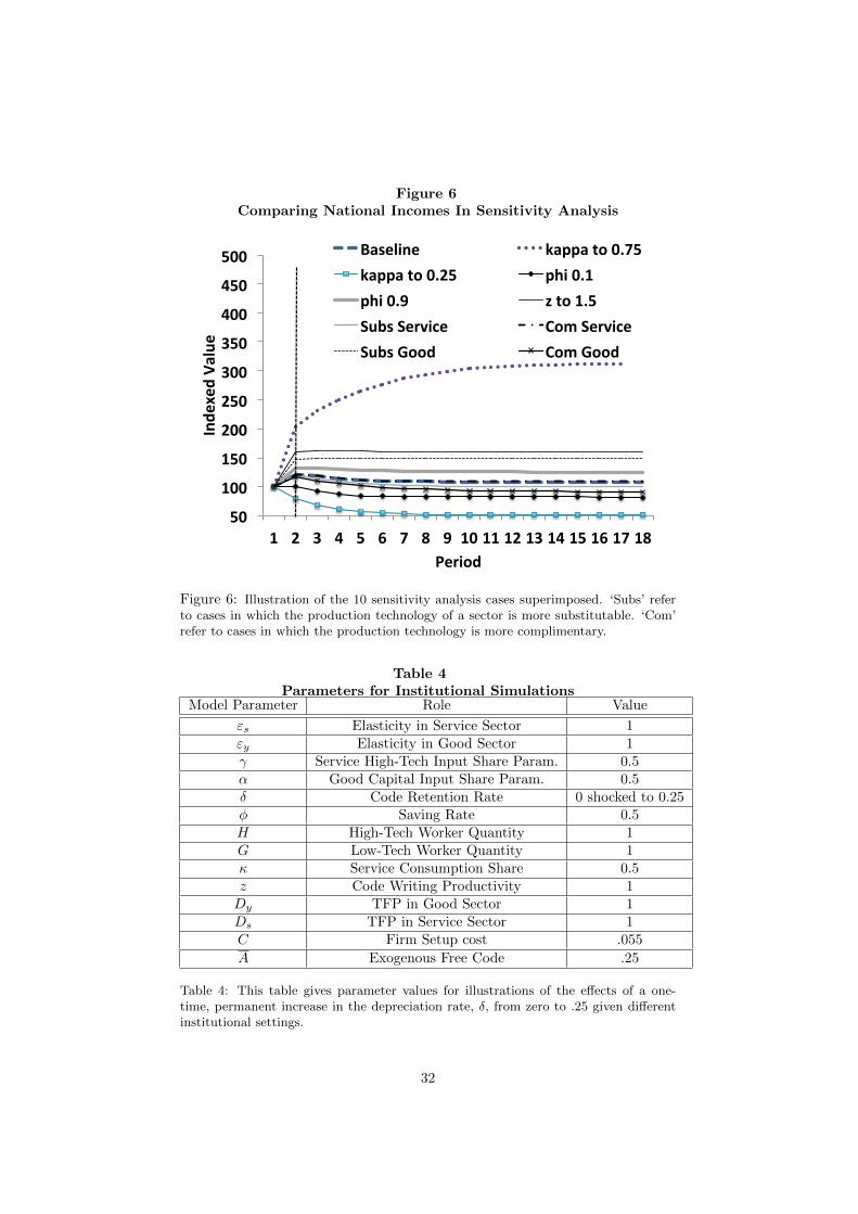
Figure 6Comparing National Incomes In Sensitivity Analysis

50#

100#

150#

200#

250#

300#

350#

400#

450#

500#

1# 2# 3# 4# 5# 6# 7# 8# 9# 10#11#12#13#14#15#16#17#18#

Inde

xed#Va

lue#

Period#

Baseline# kappa#to#0.75#kappa#to#0.25# phi#0.1#phi#0.9# z#to#1.5#Subs#Service# Com#Service#Subs#Good# Com#Good#

Figure 6: Illustration of the 10 sensitivity analysis cases superimposed. ‘Subs’ referto cases in which the production technology of a sector is more substitutable. ‘Com’refer to cases in which the production technology is more complimentary.

Table 4Parameters for Institutional Simulations

Model Parameter Role Value

εs Elasticity in Service Sector 1εy Elasticity in Good Sector 1γ Service High-Tech Input Share Param. 0.5α Good Capital Input Share Param. 0.5δ Code Retention Rate 0 shocked to 0.25φ Saving Rate 0.5H High-Tech Worker Quantity 1G Low-Tech Worker Quantity 1κ Service Consumption Share 0.5z Code Writing Productivity 1Dy TFP in Good Sector 1Ds TFP in Service Sector 1C Firm Setup cost .055

A Exogenous Free Code .25

Table 4: This table gives parameter values for illustrations of the effects of a one-time, permanent increase in the depreciation rate, δ, from zero to .25 given differentinstitutional settings.

32

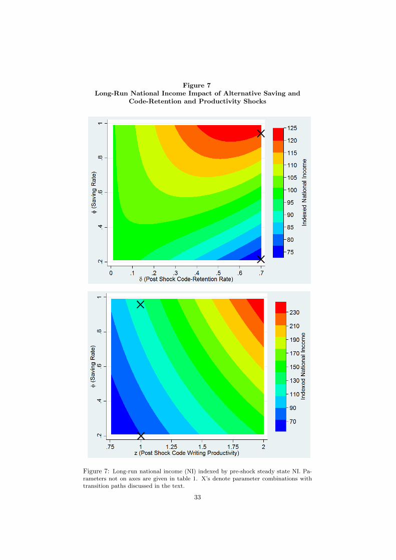
Figure 7Long-Run National Income Impact of Alternative Saving and

Code-Retention and Productivity Shocks

Figure 7: Long-run national income (NI) indexed by pre-shock steady state NI. Pa-rameters not on axes are given in table 1. X’s denote parameter combinations withtransition paths discussed in the text.

33

Figure 8Long-Run National Income Impact of Alternative Saving, Elasticity

of Substitution, and Taste Shocks

Figure 8: Long-run national income (NI) indexed by pre-shock steady state NI. Pa-rameters not on axes are given in table 2. X’s denote parameter combinations withtransition paths discussed in the text.

34

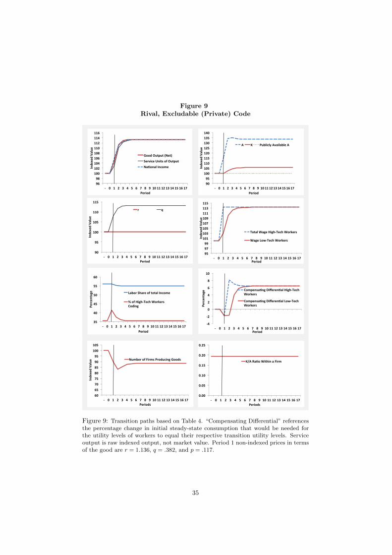
Figure 9Rival, Excludable (Private) Code

90#95#100#105#110#115#120#125#130#135#140#

)# 0# 1# 2# 3# 4# 5# 6# 7# 8# 9# 10#11#12#13#14#15#16#17#

Inde

xed#Va

lue#

#

Period#

A# K# Publicly#Available#A#

95#97#99#101#103#105#107#109#111#113#115#

)# 0# 1# 2# 3# 4# 5# 6# 7# 8# 9# 10#11#12#13#14#15#16#17#

Inde

xed#Va

lue#

#

Period#

Total#Wage#High)Tech#Workers#

Wage#Low)Tech#Workers#

90#

95#

100#

105#

110#

115#

)# 0# 1# 2# 3# 4# 5# 6# 7# 8# 9# 10#11#12#13#14#15#16#17#

Inde

xed#Va

lue#

#

Period#

r# q#

35#

40#

45#

50#

55#

60#

)# 0# 1# 2# 3# 4# 5# 6# 7# 8# 9# 10#11#12#13#14#15#16#17#

Percen

tage#

Period#

Labor#Share#of#total#Income#

%#of#High)Tech#Workers#Coding#

96#98#

100#102#104#106#108#110#112#114#116#

)# 0# 1# 2# 3# 4# 5# 6# 7# 8# 9# 10#11#12#13#14#15#16#17#

Inde

xed#Va

lue#

Period#

Good#Output#(Net)#Service#Units#of#Output#NaWonal#Income#

)4#

)2#

0#

2#

4#

6#

8#

10#

)# 0# 1# 2# 3# 4# 5# 6# 7# 8# 9# 10#11#12#13#14#15#16#17#

Percen

tage#

Period#

CompensaWng#DifferenWal#High)Tech#Workers#

CompensaWng#DifferenWal#Low)Tech#Workers#

0.00#

0.05#

0.10#

0.15#

0.20#

0.25#

)# 0# 1# 2# 3# 4# 5# 6# 7# 8# 9# 10#11#12#13#14#15#16#17#Periods#

K/A#RaWo#Within#a#Firm#

60#65#70#75#80#85#90#95#

100#105#

)# 0# 1# 2# 3# 4# 5# 6# 7# 8# 9# 10#11#12#13#14#15#16#17#

Inde

xed#Va

lue#

Periods#

Number#of#Firms#Producing#Goods#

Figure 9: Transition paths based on Table 4. “Compensating Differential” referencesthe percentage change in initial steady-state consumption that would be needed forthe utility levels of workers to equal their respective transition utility levels. Serviceoutput is raw indexed output, not market value. Period 1 non-indexed prices in termsof the good are r = 1.136, q = .382, and p = .117.

35

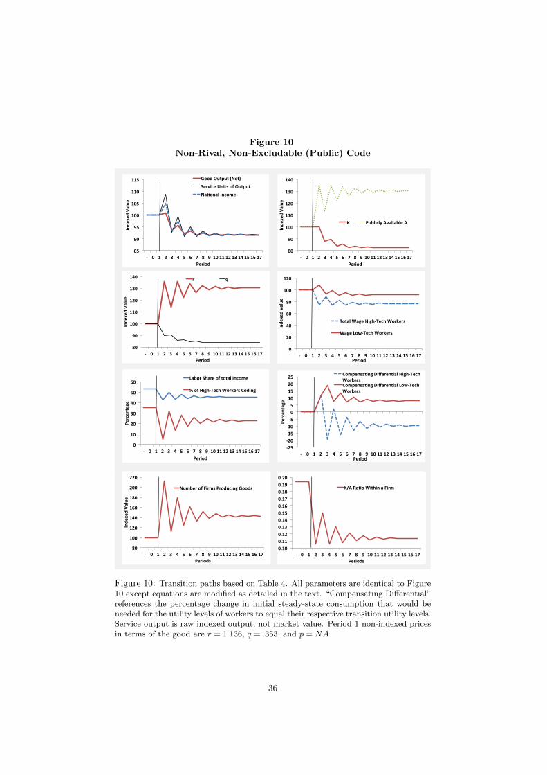
Figure 10Non-Rival, Non-Excludable (Public) Code

80#

90#

100#

110#

120#

130#

140#

)# 0# 1# 2# 3# 4# 5# 6# 7# 8# 9# 10#11#12#13#14#15#16#17#

Inde

xed#Va

lue#

#

Period#

K# Publicly#Available#A#

0#

20#

40#

60#

80#

100#

120#

)# 0# 1# 2# 3# 4# 5# 6# 7# 8# 9# 10#11#12#13#14#15#16#17#

Inde

xed#Va

lue#

#

Period#

Total#Wage#High)Tech#Workers#

Wage#Low)Tech#Workers#

80#

90#

100#

110#

120#

130#

140#

)# 0# 1# 2# 3# 4# 5# 6# 7# 8# 9# 10#11#12#13#14#15#16#17#

Inde

xed#Va

lue#

#

Period#

r# q#

0#

10#

20#

30#

40#

50#

60#

)# 0# 1# 2# 3# 4# 5# 6# 7# 8# 9# 10#11#12#13#14#15#16#17#

Percen

tage#

Period#

Labor#Share#of#total#Income#

%#of#High)Tech#Workers#Coding#

85#

90#

95#

100#

105#

110#

115#

)# 0# 1# 2# 3# 4# 5# 6# 7# 8# 9# 10#11#12#13#14#15#16#17#

Inde

xed#Va

lue#

Period#

Good#Output#(Net)#Service#Units#of#Output#NaWonal#Income#

)25#)20#)15#)10#)5#0#5#10#15#20#25#

)# 0# 1# 2# 3# 4# 5# 6# 7# 8# 9# 10#11#12#13#14#15#16#17#

Percen

tage#

Period#

CompensaWng#DifferenWal#High)Tech#Workers#CompensaWng#DifferenWal#Low)Tech#Workers#

0.10#0.11#0.12#0.13#0.14#0.15#0.16#0.17#0.18#0.19#0.20#

)# 0# 1# 2# 3# 4# 5# 6# 7# 8# 9# 10#11#12#13#14#15#16#17#Periods#

K/A#RaWo#Within#a#Firm#

80#

100#

120#

140#

160#

180#

200#

220#

)# 0# 1# 2# 3# 4# 5# 6# 7# 8# 9# 10#11#12#13#14#15#16#17#

Inde

xed#Va

lue#

Periods#

Number#of#Firms#Producing#Goods#

Figure 10: Transition paths based on Table 4. All parameters are identical to Figure10 except equations are modified as detailed in the text. “Compensating Differential”references the percentage change in initial steady-state consumption that would beneeded for the utility levels of workers to equal their respective transition utility levels.Service output is raw indexed output, not market value. Period 1 non-indexed pricesin terms of the good are r = 1.136, q = .353, and p = NA.

36

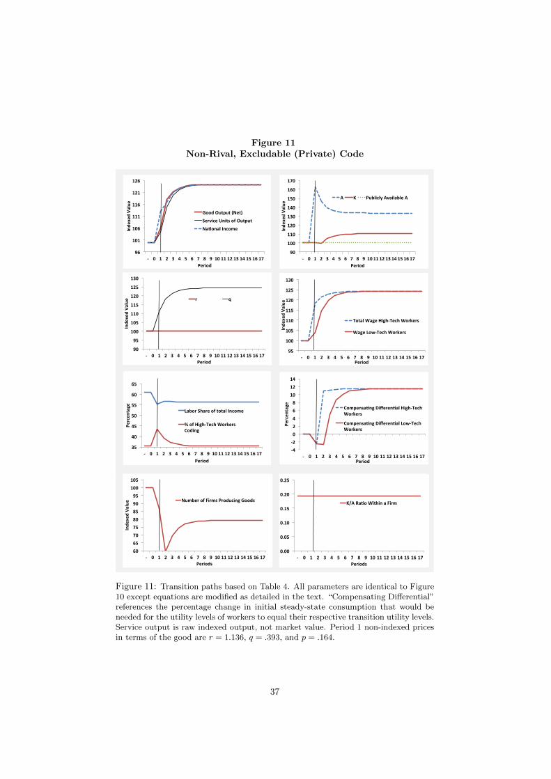
Figure 11Non-Rival, Excludable (Private) Code

90#

100#

110#

120#

130#

140#

150#

160#

170#

+# 0# 1# 2# 3# 4# 5# 6# 7# 8# 9# 10#11#12#13#14#15#16#17#

Inde

xed#Va

lue#

#

Period#

A# K# Publicly#Available#A#

95#

100#

105#

110#

115#

120#

125#

130#

+# 0# 1# 2# 3# 4# 5# 6# 7# 8# 9# 10#11#12#13#14#15#16#17#

Inde

xed#Va

lue#

#

Period#

Total#Wage#High+Tech#Workers#

Wage#Low+Tech#Workers#

90#

95#

100#

105#

110#

115#

120#

125#

130#

+# 0# 1# 2# 3# 4# 5# 6# 7# 8# 9# 10#11#12#13#14#15#16#17#

Inde

xed#Va

lue#

#

Period#

r# q#

35#

40#

45#

50#

55#

60#

65#

+# 0# 1# 2# 3# 4# 5# 6# 7# 8# 9# 10#11#12#13#14#15#16#17#

Percen

tage#

Period#

Labor#Share#of#total#Income#

%#of#High+Tech#Workers#Coding#

96#

101#

106#

111#

116#

121#

126#

+# 0# 1# 2# 3# 4# 5# 6# 7# 8# 9# 10#11#12#13#14#15#16#17#

Inde

xed#Va

lue#

Period#

Good#Output#(Net)#Service#Units#of#Output#NaWonal#Income#

+4#+2#0#2#4#6#8#

10#12#14#

+# 0# 1# 2# 3# 4# 5# 6# 7# 8# 9# 10#11#12#13#14#15#16#17#

Percen

tage#

Period#

CompensaWng#DifferenWal#High+Tech#Workers#

CompensaWng#DifferenWal#Low+Tech#Workers#

0.00#

0.05#

0.10#

0.15#

0.20#

0.25#

+# 0# 1# 2# 3# 4# 5# 6# 7# 8# 9# 10#11#12#13#14#15#16#17#Periods#

K/A#RaWo#Within#a#Firm#

60#65#70#75#80#85#90#95#

100#105#

+# 0# 1# 2# 3# 4# 5# 6# 7# 8# 9# 10#11#12#13#14#15#16#17#

Inde

xed#Va

lue#

Periods#

Number#of#Firms#Producing#Goods#

Figure 11: Transition paths based on Table 4. All parameters are identical to Figure10 except equations are modified as detailed in the text. “Compensating Differential”references the percentage change in initial steady-state consumption that would beneeded for the utility levels of workers to equal their respective transition utility levels.Service output is raw indexed output, not market value. Period 1 non-indexed pricesin terms of the good are r = 1.136, q = .393, and p = .164.

37

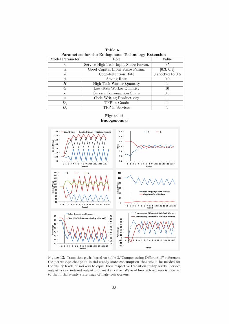
Table 5Parameters for the Endogenous Technology Extension

Model Parameter Role Value

γ Service High-Tech Input Share Param. 0.5α Good Capital Input Share Param. [0.3, 0.5]δ Code-Retention Rate 0 shocked to 0.6φ Saving Rate 0.9H High-Tech Worker Quantity 1G Low-Tech Worker Quantity 10κ Service Consumption Share 0.5z Code Writing Productivity 1Dy TFP in Goods 1Ds TFP in Services 1

Figure 12Endogenous α

0.4$

0.6$

0.8$

1.0$

1.2$

1.4$

1.6$

)$ 0$ 1$ 2$ 3$ 4$ 5$ 6$ 7$ 8$ 9$ 10$11$12$13$14$15$16$17$

Units$

Period$

A$ K$

0$

20$

40$

60$

80$

100$

120$

)$ 0$ 1$ 2$ 3$ 4$ 5$ 6$ 7$ 8$ 9$ 10$11$12$13$14$15$16$17$

Inde

xed$Value

$

Period$

Total$Wage$High)Tech$Workers$Wage$Low)Tech$Workers$

50$60$70$80$90$

100$110$120$130$140$150$

)$ 0$ 1$ 2$ 3$ 4$ 5$ 6$ 7$ 8$ 9$ 10$11$12$13$14$15$16$17$

Inde

xed$Value

$

Period$

P$ r$ q$

20$25$30$35$40$45$50$55$60$65$70$

60$

65$

70$

75$

80$

85$

90$

95$

)$ 0$ 1$ 2$ 3$ 4$ 5$ 6$ 7$ 8$ 9$ 10$11$12$13$14$15$16$17$

Percen

tage$

Period$

Labor$Share$of$total$Income$

%$of$High)Tech$Workers$Coding$(right$axis)$

)30$)20$)10$0$

10$20$30$40$50$60$70$

)$ 0$ 1$ 2$ 3$ 4$ 5$ 6$ 7$ 8$ 9$ 10$11$12$13$14$15$16$17$

Percen

tage$

Period$

CompensaSng$DifferenSal$High)Tech$Workers$

CompensaSng$DifferenSal$Low)Tech$Workers$

90$

100$

110$

120$

130$

140$

150$

160$

)$ 0$ 1$ 2$ 3$ 4$ 5$ 6$ 7$ 8$ 9$ 10$11$12$13$14$15$16$17$

Inde

xed$Value

$$

Period$

Good$Output$ Service$Output$ NaSonal$Income$

Figure 12: Transition paths based on table 3.“Compensating Differential” referencesthe percentage change in initial steady-state consumption that would be needed forthe utility levels of workers to equal their respective transition utility levels. Serviceoutput is raw indexed output, not market value. Wage of low-tech workers is indexedto the initial steady state wage of high-tech workers.

38