robust control and applications in economic theory -...

Introduction A linear model Nonlinear systems

Robust control and applications in economic theoryIn honour of Professor Emeritus Grigoris Kalogeropoulos on the

occasion of his retirement

A. N. YannacopoulosDepartment of Statistics – AUEB

24 May 2013

A. N. Yannacopoulos – Department of Statistics AUEB

Workshop on control theory and applications: In honour of Professor Emeritus G. Kalogeropoulos


In collaboration with

I W. A. Brock (Professor Emeritus, Economics Department,Wisconsin)

I A. Xepapadeas (Professor, Department of European andInternational Economic Studies, AUEB)




Introduction

I Robust control is a very important part of stochastic control.

I In some sense it is the most realistic version of control theory:

I We wish to control a system but we do not know the exactlaw of evolution of the state process.

I What we have is a family of laws (scenarios), and we want tocontrol the worst possible scenario.

I The best policy for the worst scenario is our robust control.




I This theme has become extremely useful in economics andfinance

I T. J. Sargent, Nobel Prize in Economics 2011 has devotedmost of his research in this field.

I Furthermore robust control has interesting connections withgame theory and in particular with stochastic differentialgames.




Control




Robust control




A linear model

I Consider a spatially extended economic system, located on adiscrete set D for simplicity, with state variable xn and withstate equation:

dxn = (∑m

anmxm +∑m

bnmum)dt +∑m

cnmdwm, n ∈ D

I Stochastic fluctuations are understood in the sense of the Itotheory of stochastic integration.

I In compact form this can be expressed as

dx = (Ax + Bu) dt + Cdw

where A,B,C : `2 → `2 are linear operators, related to thedoubly infinite matrices with elements anm,bnm, cnm,respectively.

I This can be understood as an infinite dimensionalOrnstein-Uhlenbeck equation on the Hilbert space `2.




1 · · · · · ·

2

3

i

N

j

w12

w21w2j

w23

w32

w3i

...w3N

wi3

wij

wN3

wj2

wji

...

Figure: An illustration of the spatial economy.




I The operator A gives us the interconnection of the variouseconomic units with each other.

I The operator B gives us how a control which is applied at sitem affects the state of the system at site n.

I The operator C is the covariance operator, and tells us howuncertainty at site m affect the state of the system at site n.

I Of course in the finite dimensional case the model makesperfect sense and all the above operators become matrices.

I Our model can be a model for e.g. a spatially extended fishery:x is biomass at various compartments, u is harvesting rate.




I Assume now that there is some uncertainty concerning the“true” statistical distribution of the state of the system.

I This corresponds to a family of probability measures Q suchthat each Q ∈ Q corresponds to an alternative stochastic model(scenario) concering the state of the system.

I We restrict to measures Q ∼ P such that the Radon-Nikodymderivatives dQ/dP are defined through an exponentialmartingale of the type employed in Girsanov’s theorem,

dQ

dP

∣∣∣∣FT

= exp

(∫ T

0

∑n

vn(t)dwn(t)− 1

2

∫ T

0

∑n

v 2n (t)dt

)

where v = vn, n ∈ Z is an `2-valued stochastic process whichis measurable with respect to the filtration Ft satisfying theNovikov condition.




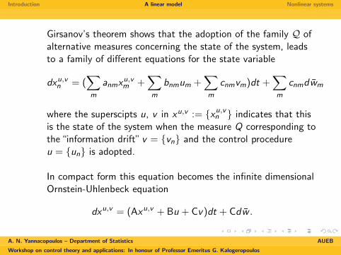
Girsanov’s theorem shows that the adoption of the family Q ofalternative measures concerning the state of the system, leadsto a family of different equations for the state variable

dxu,vn = (

∑m

anmxu,vm +

∑m

bnmum +∑m

cnmvm)dt +∑m

cnmdwm

where the superscipts u, v in xu,v := xu,vn indicates that this

is the state of the system when the measure Q corresponding tothe “information drift” v = vn and the control procedureu = un is adopted.

In compact form this equation becomes the infinite dimensionalOrnstein-Uhlenbeck equation

dxu,v = (Axu,v + Bu + Cv)dt + Cdw .




I For a fixed model v the decision maker solves the controlproblem

minu

EQ

[∫ ∞0

e−rt(〈Pxu,v (t), xu,v (t)〉+ 〈Qu(t), u(t)〉)dt

]subject to the dynamic constraints

dxu,v = (Axu,v + Bu + Cv)dt + Cdw , xu,v (0) = x0.

where 〈·, ·〉 is the inner product in the Hilbert space `2 andP,Q : `2 → `2 are symmetric positive operators, modellingdistance from a “target” and cost of control.

I This will provide a solution leading to a value function V (x0; v);corresponding to the minimum deviation obtained for the modelQv under the minimum possible effort.




I Being uncertain about the true model, the decision maker willopt to choose this strategy that will work in the worst casescenario; this being the one that maximizes V (x0; v), theminimum over all u having chosen v , over all possible choicesfor v .

I The robust control problem to be solved is of the general form

minu

maxv

EQ

[∫ ∞0

e−rt(〈(Pxu,v )(t), xu,v (t)〉+ 〈(Qu)(t), u(t)〉 − θ〈(Rv)(t), v(t)〉)dt],

subject to the dynamic constraint

dxu,v = (Axu,v + Bu + Cv)dt + Cdw , xu,v (0) = x0.

where θ > 0 and R = rnm is a symmetric positive operator.

I The third term corresponds to a quadratic loss function relatedto the “cost” of model misspecification.




Quadratic loss functions are rather common in statistical decisiontheory, mainly on account of their connection with theKullback-Leibler entropy of the two measures.

Proposition

The robust optimization problem is related to a robust controlproblem with an entropic constraint of the form

infu

supQ∈Q

EQ

[∫ ∞0

e−rt(〈Px(t), x(t)〉+ 〈Qu(t), u(t)〉)dt

],

subject to H(P | Q) =

∫Ω

ln

(dQ

dP

)dQ < H0

and the dynamic constraint.

θ plays the role of the Lagrange multiplier for the entropicconstraint.




Connection with stochastic differential games

I One particularly intuitive way of viewing this problem is as atwo player game:

I The first player is the decision maker while the second player isan adversarial agent (nature) who has “control” over theuncertainty.

I The first player chooses her actions so as to minimize thedistance of the state of the system from a chosen target at theminimum possible cost, whereas the second player is aconsidered by the first player as a malevolent player who tries to“mess up” the first players efforts.

I This results to the interpretation of solution the robust controlproblem as a Nash equilibrium of this game.




Hamilton-Jacobi-Bellman-Isaacs equation

I The solution of this stochastic differential game can be obtainedusing a generalization of the Hamilton-Jacobi-Bellman equationcalled the Hamilton-Jacobi-Bellman-Isaacs (HJBI) equation.

I This equation is a fully nonlinear PDE involving the generatoroperator which for the Ornstein-Uhlenbeck process is

LV = 〈Ax + Bu + Cv ,DV 〉+ Tr(CC∗D2V )

I Using L we construct the Hamiltonian H : `2 × `2 × `2 → Rdefined as

H(V ; x , u, v) = LV + 〈Px , x〉+ 〈Qu, u〉 − θ〈Rv , v〉




I We need to obtain the upper hamiltonian and lowerhamiltonians defined respectively as

H := supu

infvH(V ; x , u, v), H := inf

vsupuH(V ; x , u, v).

I The upper solution to the game is the solution of the HJBIequation

∂V

∂t+ sup

uinfvH(V ; x , u, v) = 0

I The lower solution of the game is the solution of the HJBIequation

∂V

∂t+ inf

vsupuH(V ; x , u, v) = 0




A version of the minimax theorem guarantees that:

Theorem

Suppose that

H(V ; x) := supu

infvH(V ; x , u, v) = inf

vsupuH(V ; x , u, v)

then a Nash equilibrium to this stochastic differential game existsand it is given by the solution of the HJBI equation

∂V

∂t+ H(V ; x) = 0

The optimal strategies are given by the maximizers and theminimizers of supu infv H(V ; x , u, v) and are given as feedbacklaws.




The solution of the linear quadratic robust control problem is givenby the following:

Theorem

The robust control problem has a solution for which the optimalcontrols are of the feedback control form

u = −Q−1B∗Hsymx , v =1

θR−1C∗Hsymx ,

and the optimal state satisfies the Ornstein-Uhlenbeck equation

dx = (A− BQ−1B∗Hsym +1

θCR−1C∗Hsym)x dt + CdW

where Hsym is the solution of the operator Riccati equation

HsymA + A∗Hsym − HsymEsymHsym − rHsym + P = 0

and Esym := 12 (E + E∗) is the symmetric part of

E := BQ−1B∗ − 1

θCR−1C∗.




The solvability and the properties of the solution for the optimalcontrol problem is reduced to the solvability and the properties ofthe solution of the operator Riccati equation.

Proposition

Let m = ||A|| defined as m = sup〈Ax , x〉, ||x ||`2 = 1 andassume that m < r/2.Then, for small enough values of ||E|| and ||P|| the operatorRiccati equation

HsymA + A∗Hsym − HsymEsymHsym − rHsym + P = 0

admits a unique bounded strong solution.




Nonlinear systems

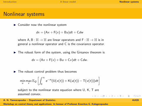
I Consider now the nonlinear system

dx = (Ax + F(x) + Bu)dt + Cdw

where A,B : H→ H are linear operators and F : H→ H is ingeneral a nonlinear operator and C is the covariance operator.

I The robust form of the system, using the Girsanov theorem is

dx = (Ax + F(x) + Bu + Cv)dt + Cdw .

I The robust control problem thus becomes

minu

maxv

EQ

[∫ ∞0

e−rt(U(x(t)) + K(u(t))− T(v(t)))dt

]subject to the nonlinear state equation where U, K, T areassumed convex.




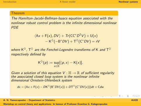
Theorem

The Hamilton-Jacobi-Bellman-Isaacs equation associated with thenonlinear robust control problem is the infinite dimensional nonlinearPDE

〈Ax + F(x),DV 〉+ Tr(CC∗D2V ) + U(x)

− K♦(−B∗DV ) + T♦(C∗DV ) = rV

where K♦, T♦ are the Fenchel-Legendre transforms of K and T♦

respectively defined by

K♦(p) := supx∈H

[〈p, x〉 − K(x)].

Given a solution of this equation V : H→ R of sufficient regularitythe associated closed loop system is the nonlinear infinitedimensional Ornstein-Uhlenbeck system

dx = (Ax + F(x)− DK♦(B∗DV (x)) + DT♦(C∗DV (x)))dt + Cdw




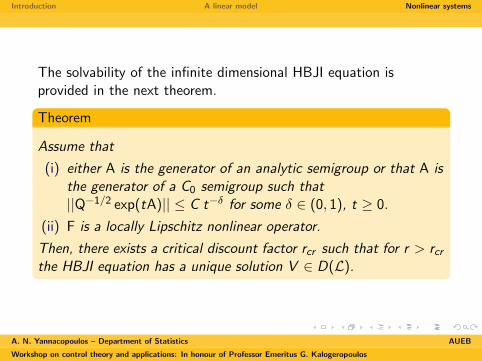
The solvability of the infinite dimensional HBJI equation isprovided in the next theorem.

Theorem

Assume that

(i) either A is the generator of an analytic semigroup or that A isthe generator of a C0 semigroup such that||Q−1/2 exp(tA)|| ≤ C t−δ for some δ ∈ (0, 1), t ≥ 0.

(ii) F is a locally Lipschitz nonlinear operator.

Then, there exists a critical discount factor rcr such that for r > rcrthe HBJI equation has a unique solution V ∈ D(L).




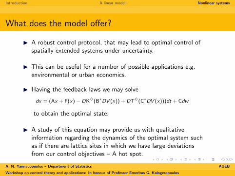
What does the model offer?

I A robust control protocol, that may lead to optimal control ofspatially extended systems under uncertainty.

I This can be useful for a number of possible applications e.g.environmental or urban economics.

I Having the feedback laws we may solve

dx = (Ax + F(x)− DK♦(B∗DV (x)) + DT♦(C∗DV (x)))dt + Cdw

to obtain the optimal state.

I A study of this equation may provide us with qualitativeinformation regarding the dynamics of the optimal system suchas if there are lattice sites in which we have large deviationsfrom our control objectives – A hot spot.




Breakdown of control: Hot spots

I What may be even more important from the conceptual pointof view is the failure of the model, rather than its success!

I Regions of important breakdown of the model are calledhotspots.

I Hotspots may arise on account of different reasons(I) Model misspecification effects are too pronounced atcertain units of the system (loss of convexity)(II) The deviation of the controlled system from the desiredtarget presents spatial variability




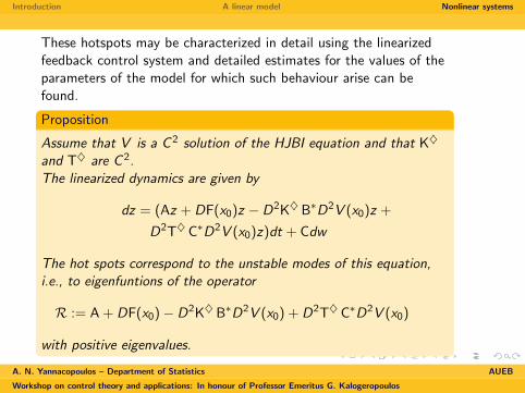
These hotspots may be characterized in detail using the linearizedfeedback control system and detailed estimates for the values of theparameters of the model for which such behaviour arise can befound.

Proposition

Assume that V is a C 2 solution of the HJBI equation and that K♦

and T♦ are C 2.The linearized dynamics are given by

dz = (Az + DF(x0)z − D2K♦ B∗D2V (x0)z +

D2T♦ C∗D2V (x0)z)dt + Cdw

The hot spots correspond to the unstable modes of this equation,i.e., to eigenfuntions of the operator

R := A + DF(x0)− D2K♦ B∗D2V (x0) + D2T♦ C∗D2V (x0)

with positive eigenvalues.




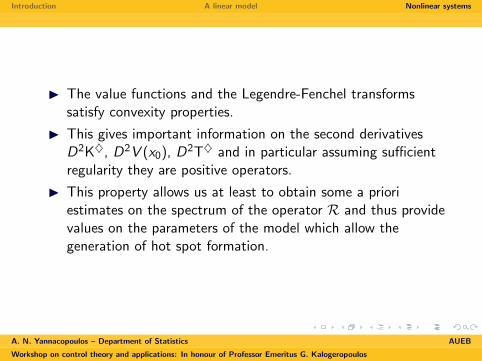
I The value functions and the Legendre-Fenchel transformssatisfy convexity properties.

I This gives important information on the second derivativesD2K♦, D2V (x0), D2T♦ and in particular assuming sufficientregularity they are positive operators.

I This property allows us at least to obtain some a prioriestimates on the spectrum of the operator R and thus providevalues on the parameters of the model which allow thegeneration of hot spot formation.




Conclusions

I Robust control is a very important field in stochastic controltheory, with interesting applications in economics.

I We have formulated and studied a robust stochastic controlproblem for a general class of interconnected systems arisingin economic modelling and provided solutions in terms of theHamilton-Jacobi-Bellman-Isaacs equation.

I An interesting phenomenon is the breakdown of control whichleads to hot spot formation.



robust control and applications in economic theory -...

Documents