robust control of mechanical systems - intech -...

0

Robust Control of Mechanical Systems

Joaquín Alvarez1 and David Rosas2

1Scientific Research and Advanced Studies Center of Ensenada (CICESE)2Universidad Autónoma de Baja California

Mexico

1. Introduction

Control of mechanical systems has been an important problem since several years ago. Forfree-motion systems, the dynamics is often modeled by ordinary differential equations arisingfrom classical mechanics. Controllers based on feedback linearization, adaptive, and robusttechniques have been proposed to control this class of systems (Brogliato et al., 1997; Slotine& Li, 1988; Spong & Vidyasagar, 1989).Many control algorithms proposed for these systems are based on models where practicalsituations like parameter uncertainty, external disturbances, or friction force terms are nottaken into account. In addition, a complete availability of the state variables is commonlyassumed (Paden & Panja, 1988; Takegaki & Arimoto, 1981; Wen & Bayard, 1988). In practice,however, the position is usually the only available measurement. In consequence, the velocity,which may play an important role in the control strategy, must be calculated indirectly, oftenyielding an inaccurate estimation.In (Makkar et al., 2007), a tracking controller that includes a new differentiable friction modelwith uncertain nonlinear terms is developed for Euler-Lagrange systems. The technique isbased on a model and the availability of the full state. In (Patre et al., 2008), a similar idea ispresented for systems perturbed by external disturbances. Moreover, some robust controllershave been proposed to cope with parameter uncertainty and external disturbances. H∞

control has been a particularly important approach. In this technique, the control objectiveis expressed as a mathematical optimization problem where a ratio between some norms ofoutput and perturbation signals is minimized (Isidori & Astolfi, 1992). It is used to synthesizecontrollers achieving robust performance of linear and nonlinear systems.In general, the control techniques mentioned before yield good control performance.However, the mathematical operations needed to calculate the control signal are rathercomplex, possibly due to the compensation of gravitational, centrifugal, or Coriolis terms,or the need to solve a Hamilton-Jacobi-Isaacs equation. In addition, if an observer is includedin the control system, the overall controller may become rather complex.Another method exhibiting good robustness properties is the sliding mode technique(Perruquetti & Barbot, 2002; Utkin, 1992). In this method, a surface in the state space ismade attractive and invariant using discontinuous terms in the control signal, forcing thesystem to converge to the desired equilibrium point placed on this surface, and making thecontrolled dynamics independent from the system parameters. These controllers display goodperformance for regulation and tracking objectives (Utkin et al., 1999; Weibing & Hung, 1993;

8

www.intechopen.com

2 Will-be-set-by-IN-TECH

Yuzhuo & Flashner, 1998). Unfortunately, they often exhibit the chattering phenomenon,displaying high-frequency oscillations due to delays and hysteresis always present in practice.The high-frequency oscillations produce negative effects that may harm the control devices(Utkin et al., 1999). Nevertheless, possibly due to the good robust performance of slidingmode controllers, several solutions to alleviate or eliminate chattering have been developedfor some classes of systems (Bartolini et al., 1998; Curk & Jezernik, 2001; Erbatur & Calli, 2007;Erbatur et al., 1999; Pushkin, 1999; Sellami et al., 2007; Xin et al., 2004; Wang & Yang, 2007).In the previous works, it is also assumed that the full state vector is available. However,in practice it is common to deal with systems where only some states are measured due totechnological or economical limitations, among other reasons. This problem can be solvedusing observers, which are models that, based on input-output measurements, estimate thestate vector.To solve the observation problem of uncertain systems, several approaches have beendeveloped (Davila et al., 2006; Rosas et al., 2006; Yaz & Azemi, 1994), including sliding modetechniques (Aguilar & Maya, 2005; Utkin et al., 1999; Veluvolu et al., 2007). The sliding modeobservers open the possibility to use the equivalent output injection to identify disturbances(Davila et al., 2006; Orlov, 2000; Rosas et al., 2006).In this chapter, we describe a control structure designed for mechanical systems to solveregulation and tracking objectives (Rosas et al., 2010). The control technique used inthis structure is combined with a discontinuous observer. It exhibits good performancewith respect to parameter uncertainties and external disturbances. Because of theincluded observer, the structure needs only the generalized position and guarantees a goodconvergence to the reference with a very small error and a control signal that reducessignificantly the chattering phenomenon. The observer estimates not only the state vectorbut, using the equivalent output injection method, it estimates also the plant perturbationsproduced by parameter uncertainties, non-modeled dynamics, and other external torques.This estimated perturbation is included in the controller to compensate the actual disturbancesaffecting the plant, improving the performance of the overall control system.The robust control structure is designed in a modular way and can be easily programed.Moreover, it can be implemented, if needed, with analog devices from a basic electroniccircuit having the same structure for a wide class of mechanical systems, making its analogimplementation also very easy (Alvarez et al., 2009). Some numerical and experimental resultsare included, describing the application of the control structure to several mechanical systems.

2. Control objective

Let us consider a mechanical system with n−degree of freedom (DOF), modeled by

M(q)q + C(q, q)q + G(q) + Φ(q, q, q)θ + γ(t) = u = τ0 + Δτ . (1)

q ∈ Rn, q = dq/dt, q = d2q/dt2 denote the position, velocity, and acceleration, respectively; M

and C are the inertia and Coriolis and centrifugal force matrices, G is the gravitational force,Φθ includes all the parameter uncertainties, and γ, which we suppose bounded by a constantσ, that is, ||γ(t)|| < σ, denotes a external disturbance. τ0 and Δτ are control inputs. Note that,under this formulation, the terms M, C, and G are well known. If not, it is known that theycan be put in a form linear with respect to parameters and can be included in Φθ (Sciavicco &Siciliano, 2000).

172 Challenges and Paradigms in Applied Robust Control

www.intechopen.com

Robust Control of Mechanical Systems 3

We suppose that τ0, which may depend on the whole state (q, q), denotes a feedback controllerdesigned to make the state (q, q) follow a reference signal (qr, qr), with an error depending onthe magnitude of the external disturbance γ and the uncertainty term Φθ, but keeping thetracking error bounded. We denote this control as the “nominal control”. We propose also toadd the term Δτ , and design it such that it confers the following properties to the closed-loopsystem.

1. The overall control u = τ0 + Δτ greatly reduces the steady-state error, provided by τ0 only,under the presence of the uncertainty θ and the disturbance γ.

2. The controller uses only the position measurement.

Note that, for the nominal control, the steady state error is normally different to zero, usuallylarge enough to be of practical value, and the performance of the closed-loop system may bepoor. The role of the additional control term Δτ is precisely to improve the performance of thesystem driven by the nominal control.The nominal control can be anyone that guarantees a bounded behavior of system (1). In thischapter we use a particular controller and show that, under some conditions, it preserves theboundedness of the state. In particular, suppose the control aim is to make the position q tracka smooth signal qr, and define the plant state as

e1 = q − qr, e2 = q − qr. (2)

Suppose also that the nominal control law is given by

τ0 = −M(·)[

Kpe1 + Kve2 − qr(t)]

+ C(·)(e2 + qr) + G(·), (3)

where Kp and Kv are n × n-positive definite matrices. However, because the velocity is notmeasured, we need to use an approximation for the velocity error, which we denote as e2 =˙q − qr. This will be calculated by an observer, whose design is discussed in the next section.Suppose that the exact velocity error and the estimated one are related by e2 = e2 + ǫ2. Then,if we use the estimated velocity error, the practical nominal control will be given by

τ0 = −M(·)(Kpe1 + Kv e2 − qr) + C(·)(e2 + qr) + G(·). (4)

Moreover, the approximated Coriolis matrix C can be given the form

C(·) = C(q, ˙q) = C(·, e2 + qr) = C(·, e2 + qr)− ΔC(·),

where ΔC = O(‖ǫ2‖). Then the state space representation of system (1), with the control law(4), is given by

e1 = e2, (5)

e2 = −Kpe1 − Kve2 + ξ(e, t) + Δu,

whereξ(·) = −M−1

[

(C − MKv)ǫ2 + ΔC(e2 + qr) + Φθ + γ]

, (6)

173Robust Control of Mechanical Systems

www.intechopen.com


and Δu = M−1(·)Δτ is a control adjustment to robustify the closed-loop system. When Δu =0, a well established result is that, if

||ξ(e, t)|| < ρ1||e||+ ρ0, ρi > 0, (7)

then there exist matrices Kp and Kv such that the state e of system (5) is bounded (Khalil,2002). In fact, the bound on the state e can be made arbitrarily small by increasing the normof matrices Kp and Kv.The control objective can now be established as design a control input Δu that, dependingonly on the position, improves the performance of the control τ0 by attenuating the effect ofparameter uncertainty and disturbances, concentrated in ξ.Note that disturbances acting on system (5) satisfy the matching condition (Khalil, 2002).Hence, it is theoretically possible to design a compensation term Δu to decouple the statee1 from the disturbance ξ. The problem analyzed here is more complicated, however, becausethe velocity is not available.In the next Section we solve the problem of velocity estimation using two observers thatguarantee convergence to the states (e1, e2). Moreover, an additional property of theseobservers will allow us to have an estimation of the disturbance term ξ. This estimatedperturbation will be used in the control Δu to compensate the actual disturbances affectingthe plant.

3. Observation of the plant state

In this section we describe two techniques to estimate the plant state, yielding exponentiallyconvergent observers.

3.1 A discontinuous observer

Discontinuous techniques for designing observers and controllers have been intensivelydeveloped recently, due to their robustness properties and, in some cases, finite-timeconvergence. In this subsection we describe a simple technique, just to show the observerperformance.The observer has been proposed in (Rosas et al., 2006). It guarantees exponential convergenceto the plant state, even under the presence of some kind of uncertainties and disturbances.Let us consider the system (5). The observer is described by

[

˙e1˙e2

]

=

[

e2 + C2ǫ1

−Kpe1 − Kv e2 + Δu + C1ǫ1 + C0sign(ǫ1)

]

, (8)

where e1 ∈ Rn and e2 ∈ R

n are the states of the observer, ǫ1 = e1 − e1. C0, C1, and C2 arediagonal, positive-definite matrices defined by

Ci = diag{ci1, ci2, . . . , cin} for i = 0, 1, 2.

The signum vector function sign(·) is defined as

sign(v) = [sign(v1), sign(v2), . . . , sign(vn)]T .


www.intechopen.com


Then, the dynamics of the observation error ǫ = (ǫ1, ǫ2) = (e1 − e1, e2 − e2), are described by

[

ǫ1

ǫ2

]

=

[

ǫ2 − C2ǫ1

−C1ǫ1 − Kvǫ2 − C0sign(ǫ1) + ξ(e, t)

]

. (9)

An important result is provided by (Rosas et al., 2006) for the case where ρ1 = 0 (seeequation (7)). Under this situation we can establish the conditions to have a convergenceof the estimated state to the plant state.

Theorem 1. (Rosas et al., 2006) If (7) is satisfied with ρ1 = 0, then there exist matrices C0, C1,and C2, such that system (9) has the origin as an exponentially stable equilibrium point. Therefore,limt→∞ e(t) = e(t).

The proof of this theorem can be found in (Rosas et al., 2006). In fact, a change of variablesgiven by v1 = ǫ1, v2 = ǫ2 − C2ǫ1, allows us to express the dynamics of system (9) by

v1 = v2, (10)

v2 = −(C1 + KvC2)v1 − (C2 + Kv)v2 − C0sign(v1) + ξ(e, t),

where v1 and v2 are vectors with the form

vi = (vi1, vi2, . . . , vin)T ; i = 1, 2.

Then system (10) can be expressed as a set of second-order systems given by

v1i = v2i,

v2i = −c1iv1i − c2iv2i − c0isign(v1i) + ξi(·), (11)

where c1i = c1i + kvic2i, c2i = c2i + kvi, for i = 1, . . . , n, and |ξi| ≤ βi, for some positiveconstants βi. The conditions to have stability of the origin are given by

c1i > 0, (12)

c2i > 0, (13)

c0i > 2λmax(Pi)

√

λmax(Pi)

λmin(Pi)

(

c1iβi

θ

)

, (14)

for some 0 < θ < 1, where Pi is a 2 × 2 matrix that is the solution of the Lyapunov equationAT

i Pi + Pi Ai = −I, and the matrix Ai is defined by

Ai =

[

0 1−c1i −c2i

]

.

System (10) displays a second-order sliding mode (Perruquetti & Barbot, 2002; Rosas et al.,2010) determined by v1 = v1 = v1 = 0. To determine the behavior of the system on thesliding surface, the equivalent output injection method can be used (Utkin, 1992), hence

v1 = −ueq + ξ(e, t) = 0, (15)


www.intechopen.com


where ueq is related to the discontinuous term C0sign(v1) of equation (10). The equivalentoutput injection ueq is then given by (Rosas et al., 2010; Utkin, 1992)

ueq = ξ(e, t). (16)

This means that the equivalent output injection corresponds to the perturbation term, whichcan be recovered by a filter process (Utkin, 1992). In fact, in this reference it is shown that theequivalent output injection coincides with the slow component of the discontinuous term in(10) when the state is in the discontinuity surface. Hence, it can be recovered using a low passfilter with a time constant small enough as compared with the slow component response, yetsufficiently large to filter out the high rate components.For example, we can use a set of n second-order, low-pass Butterworth filter to estimate theterm ueq. These filters are described by the following normalized transfer function,

Fi(s) =ω2

ci

s2 + 1.4142ωci s + ω2ci

, i = 1, . . . , n, (17)

where ωci is the cut-off frequency of each filter. Here, the filter input is the discontinuousterm of the observer, c0i

sign(v1i). By denoting the output of the filter set of as x f ∈ Rn, and

choosing a set of constants ωci that minimizes the phase-delay, it is possible to assume

limt→∞

x f = ξ(·) ≈ ξ(·), (18)

where∥

∥ξ(·)− ξ(·)∥

∥ ≤ ρ for ρ � ρ0.

3.2 An augmented, discontinuous observer

A way to circumvent the introduction of a filter is to use an augmented observer. To simplifythe exposition, consider a 1-DOF whose tracking error equations have the form of system (5).An augmented observer is proposed to be

˙e1 = w1 + c21(e1 − e1),

w1 = c11(e1 − e1) + c01sgn(e1 − e1), (19)

˙e2 = w2 + c22(w1 − e2)− Kpe1 − Kv e2 + Δu,

w2 = c12(w1 − e2) + c02sgn(w1 − e2).

If we denote the observation error as ǫ1 = e1 − e1, ǫ2 = e2 − e2, we arrive at

ǫ1 = −c21ǫ1 − w1 + e2,

w1 = c11ǫ1 + c01sgn(ǫ1), (20)

ǫ2 = −(Kv + c22)ǫ2 − w2 − c22(w1 − e2) + ξ,

w2 = c12(w1 − e2 + ǫ2) + c02sgn(w1 − e2 + ǫ2).

A change of variables given by

v11 = ǫ1,

v12 = −c21ǫ1 − w1 + e2,


www.intechopen.com


v21 = w1 − e2 + ǫ2,

v22 = v21 = −c22v21 − Kvǫ2 + w1 − e2 − w2 + ξ

converts the system to

v11 = v12,

v12 = −c11v11 − c21v12 − c01sgn(v11) + e2, (21)

v21 = v22,

v22 = −c12v21 − c22v22 − c02sgn(v21) + ξ,

where c12 = c12 − Kvc22 and ξ is a disturbance term that we suppose bounded. Under somesimilar conditions discussed in the previous section, particularly the boundedness of e2 andξ, we can assure the existence of positive constants cij such that vij converges to zero, so e1

converges to e1, w1 and e2 to e2, and w2 converges to the disturbance ξ. This observer Hencewe propose to use the redesigned control Δu, or Δτ , as (see equation (5))

Δu = −w2 → −ξ, Δτ = −M(·)w2

to attenuate the effect of disturbance ξ in system (5) or in system (1), respectively.

4. The controller

As we mentioned previously, we propose to use the nominal controller (4) because the velocityis not available from a measurement. We can use any of the observers previously described,and replace the velocity e2 by its estimation, e2. The total control is then given by

τ = τ0 + Δτ = −M(·)[

ν + Kpe1 + Kv e2 − qr(t)]

+ C(·)(e2 + qr) + G(·), (22)

where ν is the redesigned control. This control adjustment is proposed to be ν = x f , where x f

is the output of filter (17), if the first observer is used (system (8)), or ν = w2, where w2 is thelast state of system (19), if the second observer is chosen.The overall structure is shown in figure 1 when the first observer is used.A similar structure is used for the second observer. An important remark is that the nominalcontrol law (a PD-controller with compensation of nonlinearities in this case) can be chosenindependently; the analysis can be performed in a similar way. However, this nominalcontroller must provide an adequate performance such that the state trajectories remainbounded.

5. Control of mechanical systems

To illustrate the performance of the proposed control structure we describe in this section itsapplication to control some mechanical systems, a Mass-Spring-Damper (MSD), an industrialrobot, and two coupled mechanical systems which we want them to work synchronized.

5.1 An MSD system

This example illustrates the application of the first observer (equation (8), Section 3.1).Consider the MSD system shown in figure 2. Its dynamical model is given by equation (1),


www.intechopen.com


CONTROLLER PLANT

OBSERVER

FILTER

e1e2

ǫ1

γ

+

-

τ

C3sign(ǫ1)

e1qr

xf

Fig. 1. The robust control structure.

Fig. 2. Mass-spring-damper mechanical system.

with

M =

(

m1 0

0 m2

)

, C =

(

δ1 + δ2 −δ2

−δ2 δ2

)

, G =

(

(k1 + k2)x1 − k2x3

k2(x3 − x1)

)

, u =

(

τ

0

)

,

where x1 = q1, x3 = q2. Consider that parameters ki, δi, and mi, for i = 1, 2, are known. Notealso that the system is underactuated, and only one control input is driving the system at massm1. Therefore, we aim to control the position of mass 1 (x1), and consider that the action ofthe second mass is a disturbance. Hence, the model of the controlled system is again givenby equation (1), but now with M = m1, C = δ1, G = k1q. If we denote x1 = q, x2 = q, andx = (x1, x2, x3, x4) = (x1, x1, x3, x3) (see figure 2), then

Γ(x, x; θ) = Φ(x, x)θ + γ = k2(x1 − x3) + δ2(x2 − x4),


www.intechopen.com


where x3 and x4 are the solutions of the system

x3 = x4,

x4 = −k2

m2(x3 − x1)−

δ2

m2(x4 − x2),

groups the effect of uncertainty and disturbance terms Φθ + γ of equation (1).Now denote as e1 = x1 − qr, e2 = x2 − qr, then the nominal control input τ0 is proposed asequation (3), that is,

τ0 = −m1

[

Kpe1 + Kv e2 − qr(t)]

+ k1x1 + δ1 x2, (23)

where Kp and Kv are positive constants. Because the velocity is not measured, in (23) we haveused the estimation x2 = e2 + qr, delivered by the observer given by (8).With an adequate selection of the constants Kp and Kv we can guarantee that the perturbationΓ(·) in (1) is bounded (see Section 2 and (Khalil, 2002)). Therefore, from equation (16), ueq =Γ(·).Using the filter (17), we can recover an estimation of the disturbance, denoted as x f . Therefore,the redesigned control will be Δτ = m1x f which, added to (23), adjusts the nominal controlinput to attenuate the effect of the disturbance Γ.A numerical simulation was performed with plant parameter values k1 = 10

[

kgm/sec2]

,

k2 = 20[

kgm/sec2]

, δ1 = δ2 = 0.1[

kgm/sec]

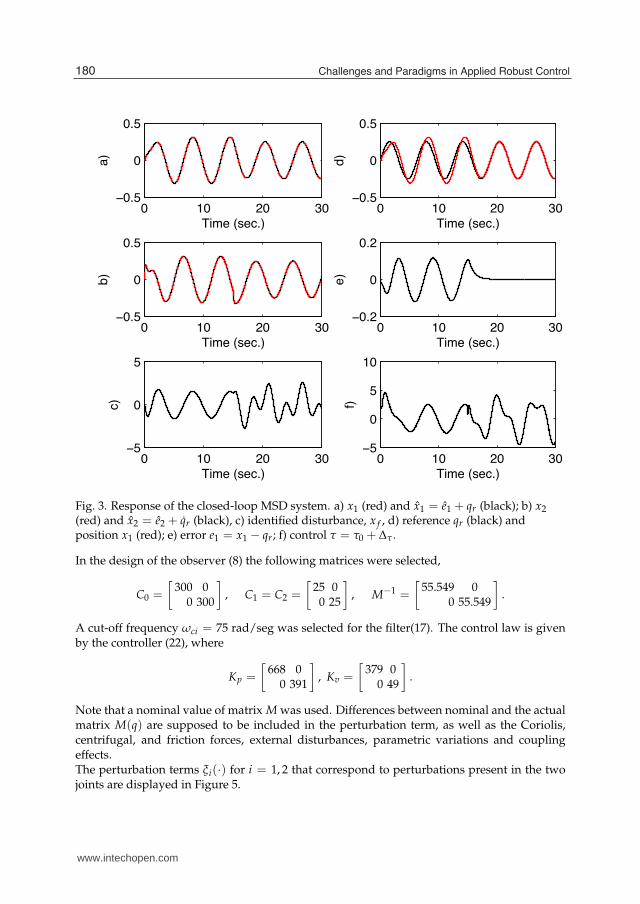
, m1 = 1 [kg], and m2 = 4 [kg]. The observerparameter values were set to c1 = 2, c2 = 2, and c0 = 3, with controller gains Kp = Kv = 10,and filter frequencies ωc = 500[rad/sec]. In this simulation the nominal control τ0 was appliedfrom 0 to 15 sec. The additional control term Δτ is activated from 15 to 30 sec. The aim is totrack the reference signal qr(t) = 0.25 sin(t).Figure 3 shows the response of this controlled system.Figures a) and b) show the convergence of the observer state to the plant state, in spite ofdisturbances produced by the mass m2. Figure c) shows the disturbance identified by thisobserver. The response of the closed-loop system is presented in Figures d), e), and f). Here wesee a tracking error when the additional control term Δτ is not present (from 0 to 15 seconds).However, when this term is incorporated to the control signal, at t = 15 sec, the tracking errortends to zero. It is important to note that, contrary to typical sliding mode controllers, thecontrol input (Figure 3.f) does not contain high frequency components of large amplitude.

5.2 An industrial robot

This is an example of the application of the first observer (Section 3.1) to a real system.In this section we show the application of the described technique to control the first twojoints of a Selective Compliant Assembly Robot Arm (SCARA), shown in figure 4, used in themanufacturing industry, and manufactured by Sony®.In this experiment we have an extreme situation because all parameters are unknown. Thecontrol algorithm was programed in a PC using the Matlab® software, and the control signalsare applied to the robot via a data acquisition card for real-time PC-based applications, theDSpace® 1104. The desired trajectory, which was the same for both joints, is a sinusoidalsignal given by qr(t) = sin(t).


www.intechopen.com


$ %$ &$ '$$#(

$

$#(

)01. !2.,#"

*"

$ %$ &$ '$$#(

$

$#(

)01. !2.,#"

+"

$ %$ &$ '$(

$

(

)01. !2.,#"

,"

$ %$ &$ '$$#(

$

$#(

)01. !2.,#"

-"$ %$ &$ '$

$#&

$

$#&

)01. !2.,#"."

$ %$ &$ '$(

$

(

%$

)01. !2.,#"

/"

Fig. 3. Response of the closed-loop MSD system. a) x1 (red) and x1 = e1 + qr (black); b) x2

(red) and x2 = e2 + qr (black), c) identified disturbance, x f , d) reference qr (black) andposition x1 (red); e) error e1 = x1 − qr; f) control τ = τ0 + Δτ .

In the design of the observer (8) the following matrices were selected,

C0 =

[

300 00 300

]

, C1 = C2 =

[

25 00 25

]

, M−1 =

[

55.549 00 55.549

]

.

A cut-off frequency ωci = 75 rad/seg was selected for the filter(17). The control law is givenby the controller (22), where

Kp =

[

668 00 391

]

, Kv =

[

379 00 49

]

.

Note that a nominal value of matrix M was used. Differences between nominal and the actualmatrix M(q) are supposed to be included in the perturbation term, as well as the Coriolis,centrifugal, and friction forces, external disturbances, parametric variations and couplingeffects.The perturbation terms ξi(·) for i = 1, 2 that correspond to perturbations present in the twojoints are displayed in Figure 5.


www.intechopen.com


Fig. 4. A SCARA industrial robot.

0 2 4 6 8 10 12 14 16 18 20

100

0

100

pert

urb

ation

join

t 1

(volts)

0 2 4 6 8 10 12 14 16 18 20100

50

0

50

100

time (sec)

pert

urb

ation

join

t 2

(volts)

Fig. 5. Identified perturbation terms in the joints of an industrial robot. Up: joint 1perturbation. Down: joint 2 perturbation.


www.intechopen.com


To verify the observer performance, the observation errors ei = θi − θi, for i = 1, 2, aredisplayed in Figure 6, showing small steady-state values.

0 2 4 6 8 10 12 14 16 18 200.5

0

0.5

positio

n e

rror

join

t 1

(rads)

0 2 4 6 8 10 12 14 16 18 200.5

0

0.5

time (sec)

positio

n e

rror

join

t 2

(rads)

Fig. 6. Observation position errors of the industrial robot.

Figure 7 shows the system output and the reference. Control inputs for joints 1 and 2 aredisplayed in Figure 8.Although these control inputs exhibit high frequency components with small amplitude, theydo not produce harmful effects on the robot. Also, it is interesting to note that the controlinput levels remain in the dynamic range allowed by the robot driver, that is, between −12 Vand +12 V.

5.3 Two synchronized mechanical systems

This example illustrates the practical performance of the proposed technique, using theaugmented observer given by (19). It refers to a basic problem of synchronization.Synchronization means correlated or corresponding-in-time behavior of two or moreprocesses (Arkady et al., 2003). In some situations the synchronization is a naturalphenomenon; in others, an interconnection system is needed to obtain a synchronizedbehavior or improve its transient characteristics. Hence, the synchronization becomesa control objective and the synchronization obtained in this way is called controlledsynchronization (Blekhman et al., 1997). Some important works in this topic are given by(Dong & Mills, 2002; Rodriguez & Nijmeijer, 2004; Soon-Jo & Slotine, 2007).In this subsection we present a simple application of the control technique to synchronize twomechanisms connected in the basic configuration, called master-slave (see figure 9).The master system is the MSD described in Section 5.1, manufactured by the company ECP®,model 210, with only the first mass activated. The slave is a torsional system from the samecompany, with the first and third disks connected. The master sends its position x to theslave, and the synchronization objective is to make the slave track the master state, that is, the


www.intechopen.com


0 2 4 6 8 10 12 14 16 18 202

1

0

1

2ra

dia

ns

0 2 4 6 8 10 12 14 16 18 202

1

0

1

2

time (sec)

radia

ns

Fig. 7. Reference signal (dotted line) and position (solid line) for each joint of the industrialrobot. Up: joint 1. Down: joint 2.

0 2 4 6 8 10 12 14 16 18 2010

5

0

5

10

contr

ol in

put

join

t 1

(volts)

0 2 4 6 8 10 12 14 16 18 203

2

1

0

1

2

3

time (sec)

contr

ol input

join

t 2

(volts)

Fig. 8. Control input for each joint of the industrial robot.


www.intechopen.com


rectilinear system (master)

torsional system (slave)

position x

Fig. 9. Two synchronized mechanisms in a master/slave configuration. The master is therectilinear system, model 210, from ECP®. The slave is the torsional system, model 205, fromthe same company.

angular position θ and velocity θ of the torsional system must follow the position x and thevelocity x of the master, respectively. The relation between the two states is 1cm of the mastercorresponds to 1rad of the slave.The rectilinear system is modeled by

mx + cm x + kmx + γm(t) = F(t),

where x is the position of the mass; m, cm, and km are the mass, damping, and springcoefficients, respectively, and F is an external force driving the system. The torsional systemis described as

Jθ1 + ct θ1 + kt(θ1 − θ2) + γt(t) = τ0 + Δτ ,

where θ1 and θ2 are the angular positions of the first and third disks, respectively; J, ct, andkt are the inertia, damping, and spring coefficients of the first disk. γm and γt are externaldisturbances possibly affecting the systems. The force driving the MSD system is set as F(t) =1.5 sin(1.5πt). All positions are available, but the velocities are estimated with the secondobserver (19) (see Section 3.2).The nominal values of the coefficients are given in Table 1.

System Parameter Value Units

MSD m 1.27 kgkm 200 N/mcm 2.1 N/m/sec

Torsional J 0.0108 Kg-m2

ct 0.007 N-m/rad/seckt 1.37 N-m/rad

Observer c11, c12, c21, c22 500c01 50c02 100

Table 1. Parameter values for the synchronization example.


www.intechopen.com


If we define the synchronization error as

e1 = x − θ, e2 = x − θ,

the control objective es to make e = (e1, e2) converge to zero.Let us consider the nominal control

τ0 = −J(kpe1 + kv e2) + ctˆθ1 + ktθ1 − ktθ2,

where ˆθ1 and e2 are the estimated velocity and the estimated velocity error obtained from theobserver. From the last equations it is possible to get the synchronization error dynamics as

e1 = e2

e2 = −kpe1 − kve2 + Δu − ξ,

where Δu = J−1Δτ and

ξ = (Jct − kv)ǫ2 + J−1γt(t)− m−1 (cm x + kmx − F(t) + γm(t)) ,

with ǫ2 = e2 − e2.We have then formulated this synchronization problem in the same framework allowing usto design a robust controller. Therefore, we can use one of the observers described previously,and use a redesign control Δτ = Jξ.We describe the results obtained from this controller to synchronize these devices. Figure 10shows its performance, using the augmented observer (19).

# % ' ) * $#%

$

#

$

%

18:6 !>"

2;8?>

/<>8?8<;>

094@6-4>?6=

# % ' ) * $#$#

(

#

(

$#

18:6 !>"

2;8?>

369<58?86>

094@6-4>?6=

# % ' ) * $#&

%

$

#

$

%

18:6 !>"

2;8?>

,==<=>

/<>8?8<;369<58?B

# % ' ) * $#%

$

#

$

%

18:6 !>"

.6A?

<;>

+<;?=<9

+<;?=<9 >87;49

Newton-m

Fig. 10. Responses of the synchronized mechanisms (Figure 9). One unit corresponds to 1 cm(1 rad) for the position, or 1 cm/sec (1 rad/sec) for the velocity, of the master (slave) system.

This figure shows how the slave (torsional) system synchronizes with the master (rectilinear)system in about 1 sec. In 2 sec the synchronization error (position and velocity) is very small.


www.intechopen.com


The control input designed for the slave is saturated at ±2 N-m, and after 1 sec maintainsits values between −1 and +1 N-m. This is accomplished even under the presence of thedisturbance introduced by the third disk, which is not modeled.

6. Conclusions

A robust control structure for uncertain Lagrangian systems with partial measurement of thestate has been presented. This control structure allows us to solve tracking and regulationproblems and guarantees the convergence to a small neighborhood of the reference signal, inspite of nonvanishing disturbances affecting the plant.This technique makes use of robust, discontinuous observers with a simple structure. Animportant property of these observers is its ability to estimate the disturbances acting on theplant, which can be conveniently incorporated in the control signal to increase the robustnessof the controller and decrease the steady-state tracking error. The observer structure caneven be built with conventional analog circuits, as it is described in (Alvarez et al., 2009).An adequate tuning of the observer parameters guarantees the convergence to the referencesignal in an operation region large enough to cover practical situations.The numerical simulations and the experimental results described in this chapter exhibiteda good performance of the proposed technique, and the control signal showed values insidepractical ranges.An interesting and important problem that has been intensively studied recently is thesynchronization of dynamical systems. Synchronization of mechanical systems is importantas soon as two or more mechanical systems have to cooperate. The control techniquedescribed in this chapter has been applied to the simplest configuration, that is, themaster/slave synchronization, exhibiting a good performance. This same control strategy,based on robust observers, can be also successfully applied to synchronize arrays ofmechanical systems, connected in diverse configurations. A more detailed application canbe found in (Alvarez et al., 2010).

7. Acknowledgement

We thank Jonatan Peña and David A. Hernandez for performing the experiments of Section5.2 and 5.3.

8. References

Aguilar, R. & Maya, R. (2005), State estimation for nonlinear systems under modeluncertainties: a class of sliding-mode observers, J. Process Contr. Vol. (15): 363-370.

Alvarez, J., Rosas, D. & Peña, J. (2009), Analog implementation of a robust control strategy formechanical systems, IEEE Trans. Ind. Electronics, Vol. (56), No. 9: 3377-3385.

Alvarez, J., Rosas, D., Hernandez, D. & Alvarez, E. (2010), Robust synchronization of arraysof Lagrangian systems, Int. J. of Control, Automation, and Systems, Vol. (8), No.5:1039-1047.

Arkady, P., Michael, R. & Kurths, J. (2003), Synchronization. A Universal Concept in NonlinearSciences, Cambridge Press: Cambridge.

Bartolini, G., Ferrara, A. & Usani, E. (1998), Chattering avoidance by second-order slidingmode control, IEEE Trans. Aut. Ctl. Vol. (43), No. 2: 241-246.


www.intechopen.com


Blekhman, I. I., Fradkov, A. L., Nijmeijer, H. & A. Y. Pogromsky, (1997) On self-synchronizationand controlled synchronization, Systems & Control Letters. (31): 299-305.

Brogliato, B., Niculescu, S. I. & Orhant, P. (1997), On the control of finite-dimensionalmechanical systems with unilateral constraints, IEEE Trans. Aut. Ctl., Vol. (42), No.2: 200-215.

Curk, B. & Jezernik, K. (2001), Sliding mode control with perturbation estimation: Applicationon DD robot mechanism, Robot. Vol. (19): 641-648.

Davila, J., Fridman, L. & Poznyak, A. (2006), Observation and identification of mechanicalsystems via second order sliding modes, Int. J. Control, Vol. (79), No. 10: 1251-1262.

Dong, S. & Mills, J. K. (2002), Adaptive synchronize control for coordination of multirobotassembly tasks, IEEE Trans. on Robotics and Automation, Vol. (18), No. 4: 498-510.

Erbatur, K., & Calli, B. (2007), Fuzzy boundary layer tuning as applied to the control of a directdrive robot, in Proc. IECON: 2858–2863.

Erbatur, K., Okyay, M. & Sabanovic, A. (1999), A study on robustness property of sliding-modecontrollers: A novel design and experimental investigations, IEEE Trans. Ind.Electron., Vol. (46), no. 5: 1012–1018.

Isidori, A., &Astolfi, A. (1992), Disturbance attenuation and H U221e control via measurementfeedback in nonlinear systems, IEEE Trans. Aut. Ctl., Vol. (37), No. 9: 1283-1293.

Khalil, H. (2002) Nonlinear Systems, New Jersey: Prentice Hall.Makkar, C., Hu, G., Sawyer, W. G. & Dixon, W. E. (2007), Lyapunov-based tracking control

in the presence of uncertain nonlinear parametrizable friction, IEEE Trans. Aut. Ctl.,Vol (52), No. 10: 1988-1994.

Orlov, I. (2000), Sliding mode observer-based synthesis of state derivative-free model referenceadaptive control of distributed parameter systems, J. Dyn. Syst-T ASME, Vol. (122),No. 4: 725-731.

Paden, B. & Panja, R. (1988). Globally asymptotically stable PD+ controller for robotmanipulators, Int. J. Control Vol (47), No. 6: 1697–1712.

Patre, P. M., MacKunis, W., Makkar, C. & Dixon, W. E. (2008), Asymptotic tracking for systemswith structured and unstructured uncertainties, IEEE Trans. Control Syst. Technol.,Vol. (16), No. 2: 373-379.

Perruquetti, W. & Barbot, J. (Eds), (2002), Sliding Mode Control in Engineering, New York:Marcel Dekker.

Pushkin, K. (1999), Existence of solutions to a class of nonlinear convergent chattering freesliding mode control systems, IEEE Trans. Aut. Ctl., Vol. (44), No. 8: 1620-1624.

Rodriguez, A. & Nijmeijer, H. (2004), Mutual synchronization of robots via estimated statefeedback: a cooperative approach, IEEE Trans. on Control Systems Technology, Vol.(12), No. 4: 542-554.

Rosas, D., Alvarez, J. & Fridman, L. (2006), Robust observation and identification of nDOFLagrangian systems, Int. J. Robust Nonlin., Vol. (17): 842-861.

Rosas, D., Alvarez, J. & Peña, J. (2010), Control structure with disturbance identification forLagrangian systems, Int. J. Non-Linear Mech., doi:10.1016/j.ijnonlinmec.2010.08.005.

Sciavicco, L. & Siciliano, B. (2000) Modelling and Control of Robots Manipulators, London:Springer-Verlag.

Sellami, A., Arzelier, D., M’hiri, R. & Zrida, J. (2007), A sliding mode control approach forsystems subjected to a norm-bounded uncertainty, Int. J. Robust Nonlin., Vol. (17):327-346.


www.intechopen.com


Slotine, J. J. & Li, W. (1988). Adaptive manipulator control: A case study, IEEE Trans. Aut. Ctl.,Vol. (33): 995-1003.

Soon-Jo, C & Slotine, E. (2007). Cooperative robot control and synchronization of Lagrangiansystems, in Proc. 46th IEEE Conference on Decision and Control, New Orleans.

Spong, M. W. & Vidyasagar, M. (1989), Robot Dynamics and Control, New York: Wiley.Takegaki, M. & Arimoto, S. (1981). A new feedback method for dynamic control manipulators,

J. Dyn. Syst. Trans. ASME, Vol (103): 119–125.Utkin, V. (1992), Sliding Modes in Control and Optimization, New York: Springer-Verlag.Utkin, V., Guldner, J. & Shi, J. (1999), Sliding Mode Control in Electromechanical Systems,

London, U.K.: Taylor & Francis.Veluvolu, K., Soh, Y. & Cao, W. (2007), Robust observer with sliding mode estimation for

nonlinear uncertain systems, IET Control Theory A., Vol. (5): 1533-1540.Xin, X. J., Jun, P. Y. & Heng, L. T. (2004), Sliding mode control whith closed-loop filtering

architecture for a class of nonlinear systems, IEEE T. Circuits-1, Vol. (51), No. 4:168-173.

Wang, X. & Yang, G. (2007), Equivalent sliding mode control based on nonlinear observer fornonlinear non-minimum-phase systems, J. Dyn. Control. Syst., Vol. (13), No. 1: 25-36.

Weibing, G. & Hung, J. C., (1993), Variable structure control of nonlinear systems: A newapproach, IEEE Trans. Ind. Electronics, Vol. (40), No. 1: 45-55.

Wen, J. & Bayard, D. (1988). New class of control law for robotic manipulators. Part 1:non-adaptive case, Int. J. Control, Vol (47), No. 5: 1361–1385.

Yaz, E. & Azemi, A. (1994), Robust/adaptive observers for systems having uncertain functionswith unknown bounds, Proc. 1994 American Control Conference, Vol. (1): 73-74.

Yuzhuo, W. & Flashner, H., (1998), On sliding mode control of uncertain mechanical systems,in Proc. IEEE Aerosp. Conf., Aspen, CO, 85–92.


www.intechopen.com

Challenges and Paradigms in Applied Robust ControlEdited by Prof. Andrzej Bartoszewicz

ISBN 978-953-307-338-5Hard cover, 460 pagesPublisher InTechPublished online 16, November, 2011Published in print edition November, 2011

InTech EuropeUniversity Campus STeP Ri Slavka Krautzeka 83/A 51000 Rijeka, Croatia Phone: +385 (51) 770 447 Fax: +385 (51) 686 166www.intechopen.com

InTech ChinaUnit 405, Office Block, Hotel Equatorial Shanghai No.65, Yan An Road (West), Shanghai, 200040, China

Phone: +86-21-62489820 Fax: +86-21-62489821

The main objective of this book is to present important challenges and paradigms in the field of applied robustcontrol design and implementation. Book contains a broad range of well worked out, recent application studieswhich include but are not limited to H-infinity, sliding mode, robust PID and fault tolerant based controlsystems. The contributions enrich the current state of the art, and encourage new applications of robustcontrol techniques in various engineering and non-engineering systems.

How to referenceIn order to correctly reference this scholarly work, feel free to copy and paste the following:

Joaquin Alvarez and David Rosas (2011). Robust Control of Mechanical Systems, Challenges and Paradigmsin Applied Robust Control, Prof. Andrzej Bartoszewicz (Ed.), ISBN: 978-953-307-338-5, InTech, Available from:http://www.intechopen.com/books/challenges-and-paradigms-in-applied-robust-control/robust-control-of-mechanical-systems

robust control of mechanical systems - intech -...

Documents