robust low-rank matrix recovery

H. C. So Semester A 2021/22

Robust Low-Rank Matrix Recovery

Chapter Intended Learning Outcomes: (i) Understand the limitation of singular value

decomposition (SVD) in low-rank matrix approximation and completion applications

(ii) Know the use of -norm in enhancing robustness to

outliers

(iii) Able to solve problems with nonsmooth and/or nonconvex functions

(iv) Able to apply robust matrix decomposition in relevant

real-world applications


Limitation of Singular Value Decomposition

Recall that truncated SVD of a given matrix is to find the best rank- matrix in the least squares (LS) sense:

That is, is computed by minimizing the sum of all components of subject to the rank constraint. If some entries of contain outliers or abnormal values, e.g., values with large magnitudes, then may not be able to accurately represent the low-rank component.


Example 1 Extract chessboard from chess pieces using truncated SVD. Here . The regular structure of the chessboard corresponds to a low-rank matrix and we set . However, the result is not satisfactory. It is because the chess pieces correspond to outlier components, and the LS method cannot yield a good solution. Also, the chess pieces cannot be well extracted from . >> img = imread('board_chess.png'); combined = im2double(rgb2gray(img)); [U,S,V] = svd(combined,'econ'); r=2; board = U(:,1:r)*S(1:r,1:r)*V(:,1:r).'; imwrite(board, 'board.png', 'png'); chess = combined-board; imwrite(chess, 'chess.png','png');


The choice of rank is crucial and is the best. :

:


Example 2 Perform image inpainting in salt-and-pepper noise. Note that this noise is sometimes seen on images, which presents itself as sparsely occurring white and black pixels, with values 255 and 0 in 8-bit integer representation, respectively. We apply ALS with rank :


Unsatisfactory performance is obtained because the LS criterion is not robust to outliers. A simple idea to deal with the outliers is to use -norm where

. The -norm criterion generalizes the LS by setting .

The -norm of a vector is defined as:

(1)

Note that (1) can also be used for and .


The special cases include

is the number of nonzero elements in . As the th power of an error term (if >1 in magnitude) is less than the squared error, hence the -norm with is less sensitive to outliers or large-magnitude components. While in the -norm, a small increase of a component from 0 makes its contribution to the norm large (close to 1 for any values other than 0). Hence minimizing the -norm means minimizing the number of nonzero elements.


Suppose . What is ? What is ?

The -norm function is convex for . While it is nonconvex for .


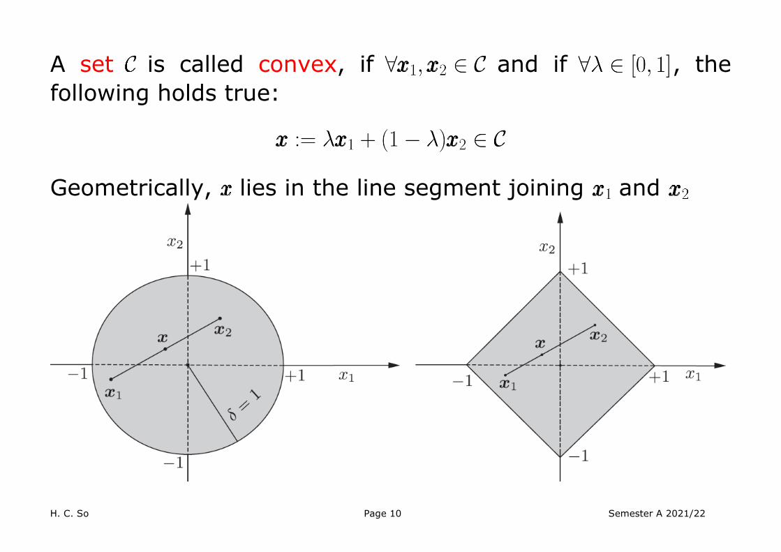
A set is called convex, if and if , the following holds true:

Geometrically, lies in the line segment joining and


Is convex? Is convex?

Is convex?


A function is called convex, if is a convex set and if , the following holds true:


In this simple case that is a quadratic function while is just any point on the -axis, it is easily seen that a convex function corresponds to a unique global minimum. This indicates that if we perform optimization on a convex function, the global solution can be easily obtained. In particular, the gradient descent is guaranteed to obtain the solution from any initial points. If a function is not convex, we call it nonconvex. If a function is nonconvex, then there are multiple minima, including the global minimum. In this case, a difficulty is that we cannot ensure if the global solution is obtained unless all minima have been checked.


A simple nonconvex function example is:

If we use gradient descent and start with , the global solution cannot be obtained.

-2 -1.5 -1 -0.5 0 0.5 1 1.5 2-4

-2

0

2

4

6

8

10

12


A function can be classified as a continuous or discontinuous function. is continuous if there are no abrupt changes in value. It is

clear that the above examples are all continuous functions as each graph is a single unbroken curve. On the other hand, an example of discontinuous function can be an investment cost function:

Source: https://www.researchgate.net/publication/231391851_Disjunctive_Programming_Techniques_for_the_Optimization_of_Process_Systems_with_Discontinuous_Investment_Costs-Multiple_Size_Regions/figures?lo=1

https://www.researchgate.net/publication/231391851_Disjunctive_Programming_Techniques_for_the_Optimization_of_Process_Systems_with_Discontinuous_Investment_Costs-Multiple_Size_Regions/figures?lo=1

https://www.researchgate.net/publication/231391851_Disjunctive_Programming_Techniques_for_the_Optimization_of_Process_Systems_with_Discontinuous_Investment_Costs-Multiple_Size_Regions/figures?lo=1


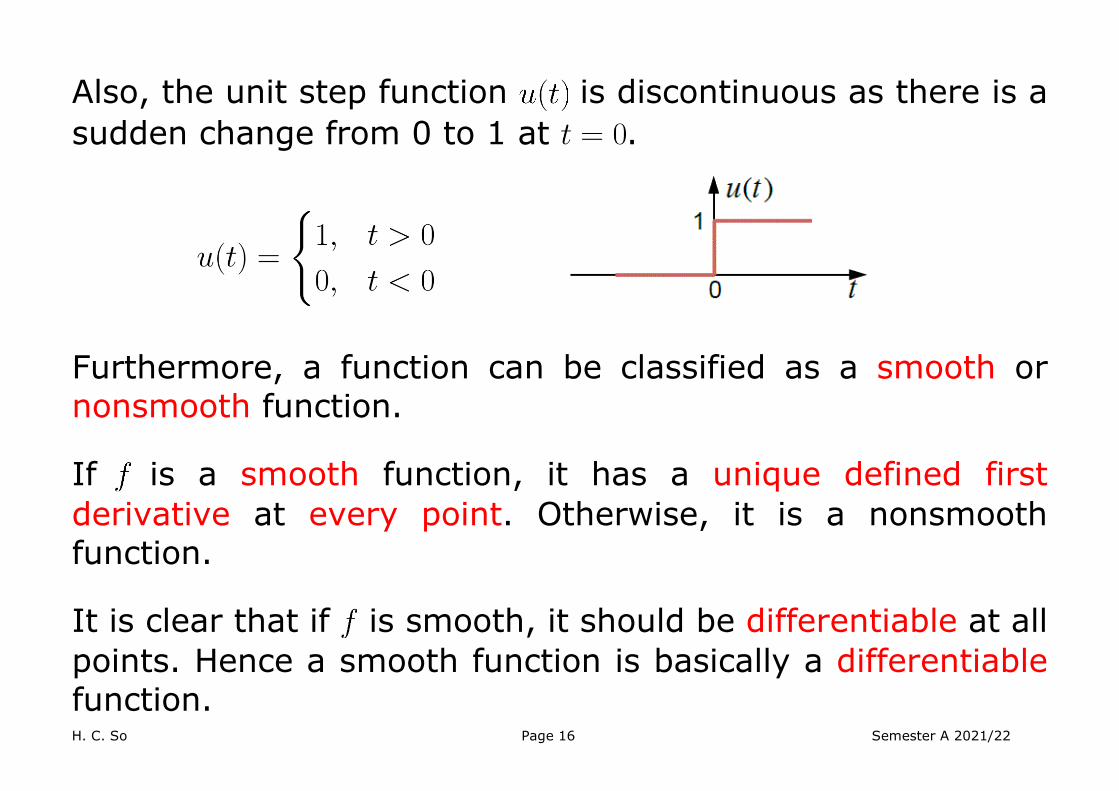
Also, the unit step function is discontinuous as there is a sudden change from 0 to 1 at .

Furthermore, a function can be classified as a smooth or nonsmooth function. If is a smooth function, it has a unique defined first derivative at every point. Otherwise, it is a nonsmooth function. It is clear that if is smooth, it should be differentiable at all points. Hence a smooth function is basically a differentiable function.


Is this function smooth or nonsmooth?

Source: https://mathematica.stackexchange.com/questions/32872/how-to-find-the-non-differentiable-points-of-a-given-continuous-function

Example 3 Examine whether the function is smooth or nonsmooth. Different values of should be considered.

https://mathematica.stackexchange.com/questions/32872/how-to-find-the-non-differentiable-points-of-a-given-continuous-function


Using chain rule:

We can see that if , the slope of is -1. On the other hand, the gradient is 1 for .

where is sign function. Combining the results, we have:

For or , is differentiable for all values of even at . Hence is smooth for .


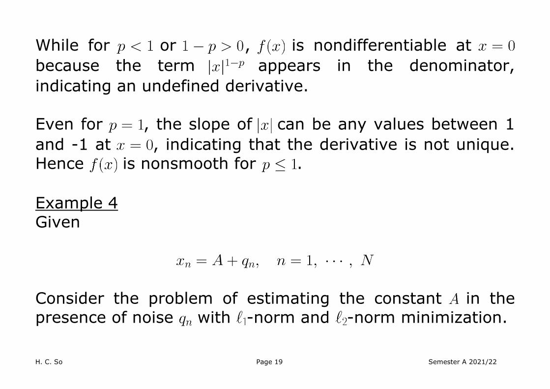
While for or , is nondifferentiable at because the term appears in the denominator, indicating an undefined derivative. Even for , the slope of can be any values between 1 and -1 at , indicating that the derivative is not unique. Hence is nonsmooth for . Example 4 Given

Consider the problem of estimating the constant in the presence of noise with -norm and -norm minimization.


The -norm minimization is in fact LS estimation:

which is simply the average. While -norm minimization, also known as least absolute deviation (LAD), refers to:

where we assign .


That is, we just arrange the values of in ascending (or descending) order, and then take the middle one. If is an even number, the median can be determined as the average of the two middlemost numbers. Suppose with , , and . We easily see that is the outlier, and the nominal value of may be around 10.

Using the LS, while using LAD, . This illustrates that in the presence of outlier-contaminated measurements, -norm minimization is able to provide a more accurate solution.


We also see that the LAD solution may not be unique because any values between 10.2 and 12.4 is a valid solution.

5 10 15 20 25 30 35 40

25

30

35

40

45

50

55

60

5 10 15 20 25 30 35 4030

40

50

60

70

80

90

100

110


Using , we get

5 10 15 20 25 30 35 40 45

25

30

35

40

45

50

55

60

65

70

75


Using , we get

5 10 15 20 25 30 35 40 45

50

100

150

200

250

300

350

400


For , -norm minimization yields a unique global minimum. We can start from any point and use gradient technique to find the minimum. While for , -norm minimization can result in multiple minima and we might use an exhaustive search to find the global minimum. If gradient technique is employed, we can obtain the global solution if the initial guess is sufficiently close to it. Otherwise, the obtained solution corresponds to a local minimum. To solve general -norm minimization problems, even for the linear cases, iterative technique is generally required. One popular method for solving -norm minimization with linear variables is the iteratively reweighted least squares (IRLS).


To understand IRLS, it may be easier to learn weighted least squares (WLS) first. Consider the linear model:

(2) where is the observation vector, is known matrix, is the parameter vector to be determined, and

contains noise. Given , the task is to find . To obtain a unique solution, we assume , i.e., the number of measurements is at least equal to the number of unknowns.


The LS cost function is constructed as:

Minimizing means that we basically assume that the noise levels of all elements in are same or even i.i.d. It is because we use the same weighting of one in each element of (or each row of ). The solution has been derived as:

(3)

However, when the elements of are not of same power and are even correlated, the WLS is able to provide a more accurate solution.


In WLS, a symmetric weighting matrix is included in the -norm cost function: (4) One basic idea is to put a larger weight where the noise level is small while a smaller weight where the noise level is large. Expanding yields:

Differentiating w.r.t. and then setting the resultant expression to 0, we get:

(5)


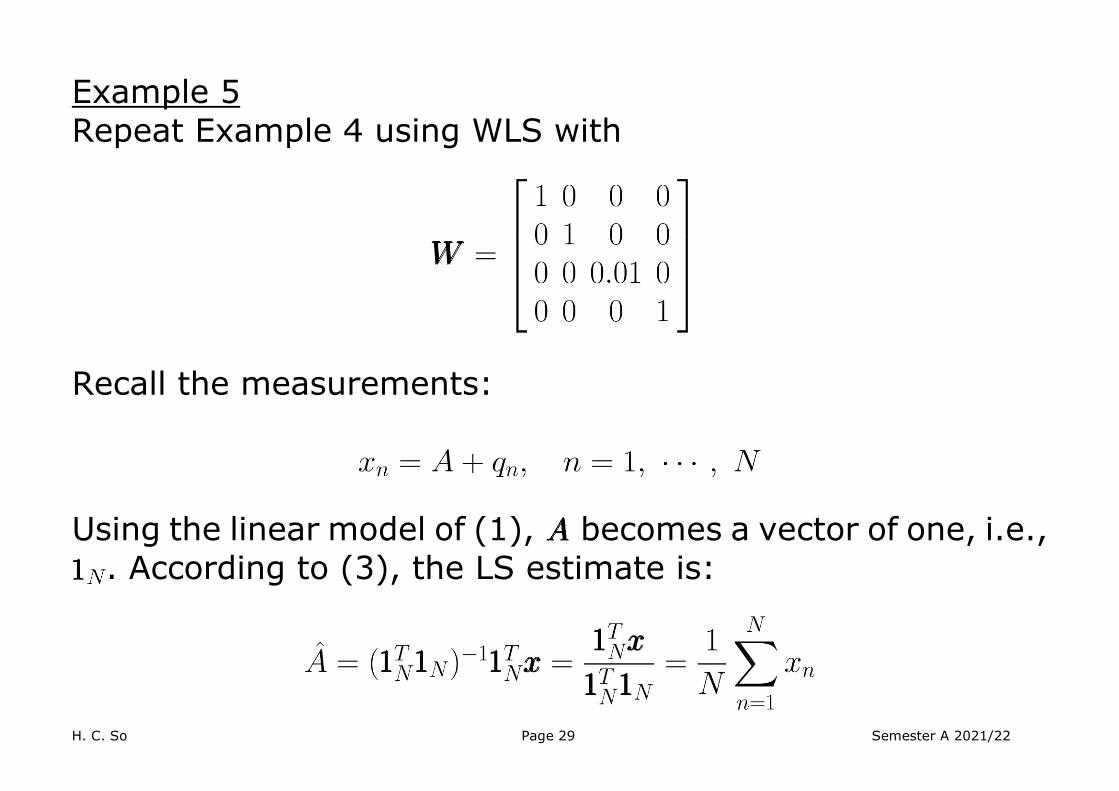
Example 5 Repeat Example 4 using WLS with

Recall the measurements:

Using the linear model of (1), becomes a vector of one, i.e.,

. According to (3), the LS estimate is:


Using (5), the WLS estimate is:

For the 4-element case, the WLS estimate is:

We see that the WLS estimate is able to provide higher accuracy than the LS and its value is comparable with the robust -norm based estimate. It is because a very small weighting is used in the measurement with possibly large noise level. In doing so, the contribution of is very small.


The -norm minimization for the linear model is:

Let the residual be:

Then can be rewritten as:

Considering as the weight in , we can write:


where

Assuming that is independent of , the WLS solution is:

Because is a function of , we estimate iteratively until convergence:

(6)


That is, we start from an initial estimate , then construct , compute , and so on.

For simplicity, can be set as random numbers or computed using the LS:

Note that for , global solution can be obtained if is sufficiently close to the global minimum. To avoid division by zero issue if , we may modify the weight as:

where is a very small value.


Example 6 Consider the problem of line fitting with data points. That is, given the measurement , which is modelled as:

where is known and is noise term. We need to find and , and then construct the line:

It is clear that the observations align with the linear model of (2):


Suppose the ideal straight line is:

Let x = 1 2 3 4 5 6 7 8 9 10 y= 3.5000 15.0000 6.5000 9.5000 6.0000 12.5000 15.5000 25.0000 18.5000 13.0000 q= 0.5000 10.0000 -0.5000 0.5000 9.0000 -0.5000 0.5000 8.0000 -0.5000 -8.0000

We use IRLS with 5 iterations initialized by the LS solution. The outliers are very strong and we see that the smaller the value of , more accurate line fitting is achieved.


: and

1 2 3 4 5 6 7 8 9 10

0

5

10

15

20

25

True

Observations

Recovered


As the -norm minimization based matrix decomposition do not provide accurate results in the presence of outliers, we can apply -norm minimization to achieve better results. A matrix measurement embedded in outliers can be modelled as:

where is the low-rank component with

and contains outliers. In image processing, may be the texture component in the image. In video processing, corresponds to the background component in the video frames.


Combining the ideas of low-rank matrix factorization and -norm minimization, we can find via

(7)

where and . The matrix -norm is defined as:

As in the ALS for recommender systems, we apply alternating minimization strategy:


For a fixed , we solve via:

Note that is dropped for notational simplicity. Hence we can find using the IRLS independently:

where is the th column of . Similarly, is computed independently using IRLS for a fixed .

To summarize, given , we estimate , , and , , in an alternative manner using the IRLS, until

convergence.


Then the low-rank component is estimated as:

If the outlier component is of interest, we can estimate it as:

When the observation matrix contains missing entries, we can easily modify the optimization cost function as: (8)

Adopting alternating minimization, matrix factorization and IRLS, -norm minimization solution can be obtained. We may say (8) generalizes the matrix factorization/recovery problem as .


Example 7 Repeat Example 1 using the -norm minimization based matrix factorization approach with and .


Example 8 Repeat Example 2 using the -norm minimization based matrix factorization approach with and .

In fact, similar results are obtained when there are no missing entries in the image:


Example 9 We consider the application of video surveillance. From two open datasets, we select the first 200 frames where each frame has dimensions of , corresponding to 76,800 pixels. Thus, the observed matrix constructed from each video is where and .

That is, we convert each frame of a video as a column of a matrix, the resultant matrix due to the background is of low-rank. Foreground objects such as moving cars or walking pedestrians, generally occupy only a fraction of the image pixels and hence can be treated as sparse outliers.

Background is and foreground is and we set the rank as .


References: 1. S. Theodoridis, Machine Learning: A Bayesian and Optimization

Perspective, Academic Press, 2015 2. http://jacarini.dinf.usherbrooke.ca/dataset2014/

http://jacarini.dinf.usherbrooke.ca/dataset2014/

robust low-rank matrix recovery

Documents