robust nonparametric detection of objects in noisy images

This article was downloaded by: [University of Connecticut]On: 11 October 2014, At: 09:01Publisher: Taylor & FrancisInforma Ltd Registered in England and Wales Registered Number: 1072954 Registeredoffice: Mortimer House, 37-41 Mortimer Street, London W1T 3JH, UK

Journal of Nonparametric StatisticsPublication details, including instructions for authors andsubscription information:http://www.tandfonline.com/loi/gnst20

Robust nonparametric detection ofobjects in noisy imagesMikhail Langovoy a & Olaf Wittich ba Max Planck Institute for Intelligent Systems , Spemannstrasse 38,D-72076 , Tübingen , Germanyb Lehrstuhl A für Mathematik, RWTH Aachen , D-52056 , Aachen ,GermanyPublished online: 13 Feb 2013.

To cite this article: Mikhail Langovoy & Olaf Wittich (2013) Robust nonparametric detectionof objects in noisy images, Journal of Nonparametric Statistics, 25:2, 409-426, DOI:10.1080/10485252.2012.759570

To link to this article: http://dx.doi.org/10.1080/10485252.2012.759570

PLEASE SCROLL DOWN FOR ARTICLE

Taylor & Francis makes every effort to ensure the accuracy of all the information (the“Content”) contained in the publications on our platform. However, Taylor & Francis,our agents, and our licensors make no representations or warranties whatsoever as tothe accuracy, completeness, or suitability for any purpose of the Content. Any opinionsand views expressed in this publication are the opinions and views of the authors,and are not the views of or endorsed by Taylor & Francis. The accuracy of the Contentshould not be relied upon and should be independently verified with primary sourcesof information. Taylor and Francis shall not be liable for any losses, actions, claims,proceedings, demands, costs, expenses, damages, and other liabilities whatsoever orhowsoever caused arising directly or indirectly in connection with, in relation to or arisingout of the use of the Content.

This article may be used for research, teaching, and private study purposes. Anysubstantial or systematic reproduction, redistribution, reselling, loan, sub-licensing,systematic supply, or distribution in any form to anyone is expressly forbidden. Terms &Conditions of access and use can be found at http://www.tandfonline.com/page/terms-and-conditions

http://www.tandfonline.com/loi/gnst20

http://www.tandfonline.com/action/showCitFormats?doi=10.1080/10485252.2012.759570

http://dx.doi.org/10.1080/10485252.2012.759570

http://www.tandfonline.com/page/terms-and-conditions

http://www.tandfonline.com/page/terms-and-conditions

Journal of Nonparametric Statistics, 2013Vol. 25, No. 2, 409–426, http://dx.doi.org/10.1080/10485252.2012.759570

Robust nonparametric detection of objects in noisy images

Mikhail Langovoya* and Olaf Wittichb

aMax Planck Institute for Intelligent Systems, Spemannstrasse 38, D-72076 Tübingen, Germany;bLehrstuhl A für Mathematik, RWTH Aachen, D-52056 Aachen, Germany

(Received 17 June 2011; final version received 12 December 2012)

We propose a novel statistical hypothesis testing method for the detection of objects in noisy images.The method uses results from percolation theory and random graph theory. We present an algorithm thatallows to detect objects of unknown shapes in the presence of nonparametric noise of unknown leveland of unknown distribution. No boundary shape constraints are imposed on the object, only a weak bulkcondition for the object’s interior is required. The algorithm has linear complexity and exponential accuracyand is appropriate for real-time systems. We prove results on consistency and algorithmic complexity ofour testing procedure. In addition, we address not only an asymptotic behaviour of the method, but also afinite sample performance of our test.

Keywords: image analysis; signal detection; image reconstruction; percolation; noisy image; nonpara-metric noise; robust testing; finite sample performance

1. Introduction

Assume we observe a noisy digital image on a screen of N × N pixels. Object detection and imagereconstruction for noisy images are two of the cornerstone problems in image analysis. In thispaper, we propose a new efficient technique for quick detection of objects in noisy images. Ourapproach uses mathematical percolation theory.

Detection of objects in noisy images is the most basic problem of image analysis. Indeed, whenone looks at a noisy image, the first question to ask is whether there is any object at all. This isalso a primary question of interest in diverse fields such as, for example, cancer detection (Ricci-Vitiani et al. 2007), automated urban analysis (Negri, Gamba, Lisini, and Tupin 2006), detectionof cracks in buried pipes (Sinha and Fieguth 2006) and other possible applications in astronomy,electron microscopy and neurology. Moreover, if there is just a random noise in the picture, itdoes not make sense to run computationally intensive procedures for image reconstruction for thisparticular picture. Surprisingly, even in those application fields where detection is the primary oreven the only question of interest, many methods solve the (more simple) detection problem notdirectly, but via the use of computationally intensive image reconstruction methods.

The crucial difference of our method is that we do not impose any shape or smoothnessassumptions on the boundary of the object. This permits the detection of non-smooth, irregu-lar or disconnected objects in noisy images, under very mild assumptions on the object’s interior.This is especially suitable, for example, if one has to detect a highly irregular non-convex objectin a noisy image. This is usually the case, for example, in the aforementioned fields of automated

*Corresponding author. Email: [email protected]

© American Statistical Association and Taylor & Francis 2013

Dow

nloa

ded

by [

Uni

vers

ity o

f C

onne

ctic

ut]

at 0

9:01

11

Oct

ober

201

4

410 M. Langovoy and O. Wittich

urban analysis, cancer detection and detection of cracks in materials. Although our detection pro-cedure works for regular images as well, it is precisely the class of irregular images with unknownshape where our method can be very advantageous.

Many modern methods of object detection, especially the ones that are used by practitionersin medical image analysis require to perform at least a preliminary reconstruction of the imagein order for an object to be detected. This usually makes such methods difficult for a rigorousanalysis of performance and for error control. Our approach is free from this drawback. We viewthe object detection problem as a nonparametric hypothesis testing problem within the class ofdiscrete statistical inverse problems. We assume that the noise density is completely unknown,and that it is not necessarily smooth or even continuous. It is possible that the noise distributiondoes not have a density.

In a recent paper Arias-Castro and Grimmett (2012), site percolation on square lattices is alsoused for cluster detection. This paper contains an extensive comparison of two percolation-basedtests with tests based on the scan statistic. A paper Arias-Castro, Donoho, and Huo (2005) startswith a similar set-up, but both of our approach and our results in Davies, Langovoy, and Wittich(2010), Langovoy and Wittich (2009) and in the present paper differ substantially from their work.We also do not use wavelet-based techniques in the present paper.

In this paper, we propose an algorithmic solution for this nonparametric hypothesis testingproblem. We prove that our algorithm has linear complexity in terms of the number of pixels onthe screen, and this procedure is not only asymptotically consistent, but on top of that has accuracythat grows exponentially with the ‘number of pixels’ in the object of detection. The algorithm hasa built-in data-driven stopping rule, so there is no need for human assistance to stop the algorithmat an appropriate step.

In this paper, we assume that pixels in and outside the object of interest have different statisticalmeans. While focusing on essentially grey scale images could have been a serious limitation inthe case of image reconstruction, it essentially does not affect the scope of applications in thecase of object detection. Indeed, in the vast majority of problems, an object that has to be detectedeither has (on the picture under analysis) a colour that differs from the background colours (e.g.in roads detection), or has the same colour but of a very different intensity, or at least an objecthas a relatively thick boundary that differs in colour from the background. Moreover, in practicalapplications one often has some prior information about colours of both the object of interest andof the background. In many of such cases, the method of the present paper is applicable aftersimple rescaling of colour values.

The paper is organised as follows. Section 2 describes in details our statistical model, and givesa necessary mathematical introduction into the percolation theory. In Section 3, the new statisticaltest is introduced and its consistency is proved. This section contains the main statistical result ofthis paper. The power of the test and the probability of false detection for the case of small imagesare studied in Section 4. In addition, in Sections 4.1 and 4.5 we describe how to select a criticalcluster size for any given finite screen size. Our approach uses the fast Newman–Ziff algorithmand is completely automatic. Our main algorithm for object detection is presented in Section 5.Appendix is devoted to the proof of two auxiliary estimates.

2. Detection and percolation

2.1. Percolation theory

This section provides the minimal necessary introduction into the mathematical percolation theory.We refer the reader to Grimmett (1999) for more information and background, as well as fornumerous graphical examples.

Dow

nloa

ded

by [

Uni

vers

ity o

f C

onne

ctic

ut]

at 0

9:01

11

Oct

ober

201

4

Journal of Nonparametric Statistics 411

Let G be an infinite graph consisting of sites s ∈ G and bonds between sites. The bonds determinethe topology of the graph in the following sense: We say that two sites s, s′ ∈ G are neighbours ifthere is a bond connecting them. We say that a subset C ⊂ G of sites is connected if for any twosites s, s′ ∈ C there are sites s1, . . . , sn such that s and s1, sn and s′, and sk and sk+1 are neighboursfor all k = 1, . . . , n − 1. Considering site percolation on the graph G means that we considerrandom configurations ω ∈ {0, 1}G where the probabilities are Bernoulli

P(ω(s) = 1) = p, P(ω(s) = 0) = 1 − p

independently for each s ∈ G, where 0 ≤ p ≤ 1 is a fixed probability. If ω(s) = 1, we say that thesite s is occupied.

Then, under mild assumptions on the graph, there is a phase transition in the qualitativebehaviour of cluster sizes. To be precise, there is a critical percolation probability pc such thatfor p < pc there is no infinite connected cluster and for p > pc there is one.

This statement and the very definition pc being the location of this phase transition are onlyvalid for infinite graphs. We cannot even speak of an infinite connected cluster for finite graphs.However, a qualitative difference of sizes of connected clusters of occupied sites can already beseen for finite graphs, say with |G| = N sites. In a sense that will be made precise below, the sizesof connected clusters are typically of order log N for small p < pc and of order N for values ofp > pc. This will yield a criterion to infer whether p is closer to zero or to one, based on observedsite configurations. Intuitively, for large enough values of N , the distinction between the tworegimes is quite sharp and located very near to the critical percolation probability of an associatedinfinite lattice.

2.2. The general detection problem

Even though this paper deals mostly with a discussion of the problem for triangular lattices, wefirst want to sketch the problem in full generality, in order to emphasise that also other choicesof the underlying lattice are possible in our processing of discretised pictures, and to make moretransparent why we decided to work with six-neighbourhoods in the present paper.

Let thus G denote a planar graph. We think of the sites s ∈ G as the pixels of a discretisedimage and of the graph topology as indicating neighbouring pixels. We consider noisy signals ofthe form

Y(s) = 1G0(s) + σε(s), (1)

where 1G0 denotes the indicator function of a subset G0 ⊆ G, the noise is given by independent,identically distributed random variables {ε(s), s ∈ G} with Eε = 0 and Vε = 1, and σ > 0 is thenoise variance. Thus, σ−1 is a measure for the signal-to- noise ratio.

Definition 1 (The detection problem) For signals of the form (1), we consider the detectionproblem meaning that we construct a test for the following hypothesis and alternative:

H0 : G0 = ∅, i.e. there is no signal.H1 : G0 �= ∅, i.e. there is a signal.

Remark (i) We usually think of these signals as being weak in the sense that the signal-to-noiseratio is small, i.e. σ−1 1. (ii) Later in this paper, we will specialise on the consideration ofsymmetric noise.

Our approach to the detection problem consists of translating the statements of hypothesis andalternative to statements from percolation theory. First of all, we choose a threshold τ ∈ R and

Dow

nloa

ded

by [

Uni

vers

ity o

f C

onne

ctic

ut]

at 0

9:01

11

Oct

ober

201

4


produce from Y a thresholded signal

Yτ (s) ={

1, Y(s) > τ ,

0, Y(s) ≤ τ .(2)

To adapt the terminology to percolation theory, we call a site s ∈ G occupied, if Yτ (s) = 1. UnderH0, the probability that a site is occupied is given by

q = P(Yτ (s) = 1) = P(ε(s) >

τ

σ

),

independently for all sites s ∈ G. That means, under H0, the thresholded signal can be equivalentlydescribed by the occupied sites in a configuration of a Bernoulli site percolation on G withpercolation probability q.

Under H1, the occupation probabilities are different for the support G0 of the signal and itscomplement G1 := G − G0. Namely,

P(Yτ (s) = 1) =

⎧⎪⎪⎨⎪⎪⎩

p0 := P

(ε >

τ − 1

σ

), s ∈ G0,

p1 := P(ε >

τ

σ

), s ∈ G1.

(3)

The basic idea is now to choose a threshold τ such that

p0 > pc > p1, (4)

where pc is a critical probability for the suitably chosen lattice G. That means the occupationprobability is supercritical on the support of the signal and subcritical outside. Under mild con-ditions on the noise distribution which will be specified below, this can always be arranged. Thisis the basic observation and the starting point for our approach to the problem stated above. Theidea is now to make use of the fact that the global behaviour of percolation clusters is qualitativelydifferent depending on whether the percolation probabilities are sub- or supercritical meaningthat there is a detectable difference in cluster formation of occupied sites according to whetherG0 = ∅, or not.

2.3. The triangular lattice and the significance of pc = 12

From the general description of the problem formulated, some immediate questions arise:

(1) How do we have to choose the threshold?(2) How does the test performance depend on the choice of the underlying lattice structure for

the discretised picture, i.e. the choice of G?(3) What can we say about the behaviour of clusters of non-occupied sites in and outside of G0?

The first question is crucial. If we do not know how to choose a threshold to achieve super- andsubcritical occupation probabilities in- and outside G0, we can still consider scales of thresholdsto determine a proper one. This will increase the computational cost of the detection. Concerningthe second question, it is important to observe that we have freedom to choose a suitable structurefor the underlying lattice. It will turn out that by choosing G to be a triangular lattice, we obtaina universal answer to question (1) and a quite satisfying result concerning question (3).

Now, we summarise the conditions on the noise distribution which will be valid throughout theentire remainder of the paper.

Dow

nloa

ded

by [

Uni

vers

ity o

f C

onne

ctic

ut]

at 0

9:01

11

Oct

ober

201

4


Noise properties. For a given graph G, the noise is given by random variables {ε(s) : s ∈ G}such that

(1) the variables ε(s) are independent, identically distributed with Eε = 0 and Vε = 1,(2) the noise distribution is symmetric,(3) the distribution of the noise is non-degenerate with respect to a critical probability pc meaning

that if F denotes the cumulative distribution function of the noise and we define

m+c = inf{x ∈ R : F(x) ≥ 1 − pc}, m−

c = sup{x ∈ R : F(x) ≤ 1 − pc},then we have m+

c = m−c where we denote the common value by m, and either

F(m) > limh→0,h>0

F(m − h), (5)

or

F ′(m) > 0. (6)

The reason to assume symmetry will become clear below. The reason to assume non-degeneracyis the following simple observation.

Lemma 1 Under the non-degeneracy condition, we can always find a threshold τ such thatwe have

p0 > pc > p1

for the probabilities p0, p1 defined in Equation (3). This holds independently of the value σ > 0of the signal-to-noise level.

Proof By Equation (3), we have p0 = 1 − F((τ − 1)/σ ) and p1 = 1 − F(τ/σ ). Choosing nowτ = σ m + 1

2 , we obtain

τ − 1

σ< m <

τ

σ.

Under the conditions (5) and (6), that implies

F( τ

σ

)> 1 − pc > F

(τ − 1

σ

).

�

In order to adapt the percolation theory terminology to the needs of image analysis, in the sequelwe will call occupied sites black and non-occupied sites white for obvious reasons. The probabilitythat a pixel (site) is white (not occupied) is given by

P(Yτ (s) = 0) =

⎧⎪⎪⎨⎪⎪⎩

1 − p0 = P

(ε ≤ τ − 1

σ

), s ∈ G0,

1 − p1 = P(ε ≤ τ

σ

), s ∈ G1.

To address question (3) above, it would be favourable that the white pixels enjoy the same propertyas the black ones, just the other way round, namely that their probabilities are supercritical outsidethe support of the signal and subcritical inside. This will be the case if we can choose τ such thatp0 > max{pc, 1 − pc} ≥ min{pc, 1 − pc} > p1. A situation where this can be done and where,furthermore, we obtain a value for τ for free is provided by the following simple but crucialobservation.

Dow

nloa

ded

by [

Uni

vers

ity o

f C

onne

ctic

ut]

at 0

9:01

11

Oct

ober

201

4


Proposition 1 Let G be a lattice such that pc = 12 and choose τ = 1

2 . If the distribution of thenoise is symmetric, we have for the threshold signal Yτ :

(1) The probability that a given pixel s is black is subcritical for s ∈ G1 and supercritical fors ∈ G0.

(2) The probability that a given pixel s is white is subcritical for s ∈ G0 and supercritical fors ∈ G1.

Proof Note first that due to the symmetry of the noise distribution, the non-degeneracy conditions(5) and (6) reduce to

F ′(0) > 0, limh→0,h>0

F(−h) < F(0).

Thus, if pc = 12 and the noise is symmetric we have

p0 = P

(ε >

τ − 1

σ

)= P

(ε > −1

2σ

)= P

(ε <

1

2σ

)> P(ε ≤ 0) ≥ 1

2= pc.

Hence, we also have p1 = P(ε > τσ) = P(ε > 1

2σ) ≤ 1 − P(ε < 12σ) = 1 − p0 < 1 − pc = 1

2and thus

p0 > max{pc, 1 − pc} = pc = min{pc, 1 − pc} > p1.

That proves the statement. �

Remark Note that, so far, the considerations are completely nonparametric with respect to thenoise. Apart from the condition for expectation and variance, we do not assume anything elseabout the cumulative distribution function F of the noise except the non-degeneracy conditionand symmetry.

We round up the discussion in this section by the statement that there actually is an examplefor a lattice with pc = 1

2 .

Definition 2 The (infinitely elongated) planar triangular lattice is the infinite graph T ⊂ C in thecomplex plane with edges (sites) given by the elements of the additive subgroup (S, +) ⊂ (C, +)

generated by the sixth roots of unity

U := {ρ ∈ C : ρ6 = 1}.Two sites s, s′ ∈ S are connected by a bond, thus they are neighbours, if and only if their Euclideandistance in the plane is d(s, s′) = 1.

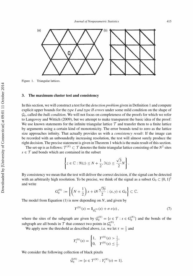
Figure 1 illustrates both the canonical embedding of the triangular lattice given in Definition 2and one other convenient imbedding of this lattice.

Proposition 2 The critical percolation probability for the planar triangular lattice is given bypc = 1

2 .

Proof See Kesten (1982, p. 52f). �

To give an example, the square lattice has several axes of symmetry, and this lattice is oftenconsidered as the most natural one for the analysis of pixelised images. However, for the sitepercolation on this lattice pc �= 1

2 ; in fact, pc ≈ 0.59. For our method this implies that, when onedecides to use the square lattice instead of the triangular one, there would be no universal thresholdthat makes our test consistent.

Dow

nloa

ded

by [

Uni

vers

ity o

f C

onne

ctic

ut]

at 0

9:01

11

Oct

ober

201

4


Figure 1. Triangular lattices.

3. The maximum cluster test and consistency

In this section, we will construct a test for the detection problem given in Definition 1 and computeexplicit upper bounds for the type I and type II errors under some mild condition on the shape ofG0, called the bulk condition. We will not focus on completeness of the proofs for which we referto Langovoy and Wittich (2009), but we attempt to make transparent the basic idea of the proof:We use known statements for the infinite triangular lattice T and transfer them to a finite latticeby arguments using a certain kind of monotonicity. The error bounds tend to zero as the latticesize approaches infinity. That actually provides us with a consistency result: If the image canbe recorded with an unboundedly increasing resolution, the test will almost surely produce theright decision. The precise statement is given in Theorem 1 which is the main result of this section.

The set-up is as follows: T (N) ⊂ T denotes the finite triangular lattice consisting of the N2 sitess ∈ T and bonds which are contained in the subset{

z ∈ C : (z) ≤ N + 1

2, �(z) ≤

√3

2N

}.

By consistency we mean that the test will deliver the correct decision, if the signal can be detectedwith an arbitrarily high resolution. To be precise, we think of the signal as a subset G0 ⊂ [0, 1]2

and write

G(N)0 :=

{(N + 1

2

)x + iN

√3y

2: (x, y) ∈ G0

}⊂ C.

The model from Equation (1) is now depending on N , and given by

Y (N)(s) = 1G(N)0

(s) + σ ε(s) , (7)

where the sites of the subgraph are given by G(N)0 = {s ∈ T : s ∈ G(N)

0 } and the bonds of thesubgraph are all bonds in T that connect two points in G(N)

0 .We apply now the threshold as described above, i.e. we let τ = 1

2 and

Y (N)τ (s) =

{1, Y (N)(s) > 1

2 ,

0, Y (N)(s) ≤ 12 .

We consider the following collection of black pixels

G(N)0 := {s ∈ T (N) : Y (N)

τ (s) = 1}.

Dow

nloa

ded

by [

Uni

vers

ity o

f C

onne

ctic

ut]

at 0

9:01

11

Oct

ober

201

4


As a side remark, note that one can view G(N)0 as an (inconsistent) pre-estimator of G(N)

0 . Now recallthat we want to construct a test on the basis of this estimator for the hypotheses H(N)

0 : G(N)0 = ∅

against the alternative H(N)1 : G(N)

0 �= ∅.

Definition 3 (The Maximum Cluster Test) Let φ(N) be a suitably chosen threshold dependingon N. Let the test statistic T be the size of the largest connected black cluster C ⊂ G(N)

0 . We rejectH(N)

0 if and only if T ≥ φ(N).

For this test, we have the following consistency result under the assumption that the support ofthe indicator function satisfies the following very weak type of a shape constraint.

Definition 4 (The Bulk Condition) We say that the support G(N)0 of the signal contains a square

of side length ρ(N) ≤ N if there is a site s ∈ G(N)0 such that s + T (ρ(N)) ⊂ G(N)

0 .

Remark If the subset G0 ⊂ [0, 1]2 contains a square of side length a > 0, the respective supportG(N)

0 contains squares of side lengths approximately ρ(N) ≈ aN .

Theorem 1 For the maximum cluster test, we have

(1) There is some constant K0 > 0 such that for φ(N) = K0 log N , we have for the type I error

limN→∞ α(N) = 0.

(2) Let φ(N) be as above. Let the support G(N)0 of the signal contain squares of side length ρ(N).

If ρ(N) ≥ K0 log N , we have for the type II error

limN→∞ β(N) = 0.

In particular, in the limit of arbitrary large precision of sampling, the test will always producethe right detection result.

Remark The method of this paper aims at detecting objects under minimal assumptions on theirshapes, so the bulk condition of Definition 4 is the only shape-related assumption that we impose.Even with this weak assumption, we still obtain an asymptotically consistent test. However, itseems that one can construct more powerful tests by imposing extra assumptions on the shapeof the object. For example, there are major advantages in detection of convex-shaped regions inpixelised images, see Huo and Ni (2009).

By the previous result, we can detect a signal correctly for virtually every noise level if we canchoose an arbitrarily high resolution. To prove this result, we will have to collect some facts frompercolation theory to make precise the intuitive idea explained in the preceding section: clustersizes are significantly larger in the supercritical regime.

We begin with the classical Aizenman–Newman theorem and transfer it step-by-step to finitelattices.

Proposition 3 (Aizenman–Newman Theorem) Consider percolation with subcritical probabil-ity p < pc = 1

2 on the infinite triangular lattice T . Then, there is a constant λ(p) > 0 dependingon p such that

P(|C| ≥ n) ≤ e−n λ(p) (8)

for all n ≥ 1, where C denotes the black cluster containing the origin.

Dow

nloa

ded

by [

Uni

vers

ity o

f C

onne

ctic

ut]

at 0

9:01

11

Oct

ober

201

4


Proof See Kesten (1982). �

Note that this result holds for the infinite triangular lattice and that we have to investigate itsconsequences for the finite lattices T (N). We do this by means of a classical monotonicity resultknown as the FKG inequality. To state this inequality, we first have to define what we mean byincreasing events.

Definition 5 We can introduce a partial ordering on the set � = {0, 1}T of all percolationconfigurations by

ω1 � ω2 :⇐⇒ ω1(s) ≤ ω2(s) for all s ∈ T .

Now we say that an event A ⊂ � is increasing if we have for the corresponding indicator variablethe inequality

1A(ω1) ≤ 1A(ω2),

whenever ω1 � ω2. The term decreasing event is defined analogously.

Now, the FKG inequality reads as follows.

Proposition 4 (FKG inequality) If A and B are both increasing (or both decreasing) events,then we have

P(A ∩ B) ≥ P(A)P(B).

Proof Fortuin, Kasteleyn, and Ginibre (1971). �

We will now apply this result to compute an estimate of the amount of wrong classificationsof points caused by the noise for detection of G(N)

0 ⊂ T (N) in a finite lattice. To be precise, weconsider the event F(N)(n) that among the sites of a configuration ω ∈ � that are erroneouslymarked black on T (N), i.e.

E(N)(ω) := {s ∈ T (N) − G(N)0 : Yτ (s) = 1}

and C(N)(ω) ⊂ E(N)(ω) the largest connected cluster, then

F(N)(n) := {ω ∈ � : |C(N)| ≥ n}.Denote now by p1 the error probability

p1 := P(Yτ (s) = 1 | s /∈ G(N)0 ),

which only depends on the noise distribution and not on N or the particularly chosen site s /∈ G(N)0 .

The consequence of the Proposition 4 for the finite lattice reads now as follows.

Proposition 5 Suppose that 0 < p1 < 12 is subcritical. Let φ(N) ≤ N be a cluster size threshold

value, and suppose that φ(N) = C log N2 and Cλ(p1) > 1, where λ(p1) > 0 is the value for theinfinite lattice from Equation (8). Then, we have

P(|C(N)| ≥ n) = N−2(Cλ(p1)−1) + O(N−4(Cλ(p1)−1))

as N tends to infinity.

Dow

nloa

ded

by [

Uni

vers

ity o

f C

onne

ctic

ut]

at 0

9:01

11

Oct

ober

201

4


Definition 6 Let T (N) ⊂ T be as above. A subset π = {s1, . . . , sn} of black sites sk ∈ T (N) with

(1) sk and sk+1 are neighbouring sites for all k = 1, . . . , n − 1,(2) 0 ≤ (s1) ≤ 1

2 ,(3) N ≤ (sn) ≤ N + 1

2

is called a left–right crossing.

Proposition 6 Consider site percolation on T (N) ⊂ T with supercritical percolation probabilityp > 1

2 . Denote by AN the event that there is some left–right crossing in T (N). Then, there is aconstant D(p) > 0 such that

P(AN ) ≥ 1 − Ne−D(p)N .

Proof The proof is analogous to the one of the corresponding statement for bond percolation inGrimmett (1999). See Langovoy and Wittich (2009) for more information. �

Proof of Theorem 1 (i) By Proposition 1, the probability p = p1 for a pixel to be black is sub-critical under the null hypothesis. Let λ(p) be the exponential factor for the infinite lattice inEquation (8). Choosing now K0 = 2C with Cλ(p1) > 1 means that by Proposition 5 the type Ierror probability tends to zero as N tends to infinity.

(ii) Let the alternative be true and G(N)0 �= ∅ contain a square of side length ρ(N). Again by

Proposition 1, the probability pB > 12 that a site is (correctly) marked black is supercritical for sites

inside the square. Therefore, the probability to find a left–right crossing π is given by Proposition 6to be

P(Aρ(N)) ≥ 1 − ρ(N) e−D(pB)ρ(N).

But every left–right crossing is a connected cluster of size at least ρ(N). Hence,

P(T ≥ ρ(N)) ≥ 1 − ρ(N) e−D(pB)ρ(N),

and together with ρ(N) ≥ K0 log N this implies that

limN→∞ P(T ≥ K0 log N) ≥ lim

N→∞ P(T ≥ ρ(N)) = 1

and thus limN→∞ β(N) = 0. �

Finally, as an addition to Proposition 5, we prove that under the same conditions, slightlychanged arguments yield an exponential estimate for the tail probabilities of the cluster sizedistribution.

Proposition 7 Suppose that 0 < p1 < 12 is subcritical. Let φ(N) ≤ N be a cluster size threshold

value with φ(N) = C log N2 and Cλ(p1) > 1, where λ(p1) > 0 is the value for the infinite latticefrom Equation (8). Then, there exists a constant K (N) > 0 such that

P(F(N)(n)) ≤ e−K (N)n

for all n ≥ φ(N).

For the case of bond percolation, much finer results were proved in Grimmett (1985). Theseresults can be directly transferred to the case of site percolation. We include Proposition 7 here forcompleteness, as the simplest necessary result of this kind formulated directly for site percolation.

Dow

nloa

ded

by [

Uni

vers

ity o

f C

onne

ctic

ut]

at 0

9:01

11

Oct

ober

201

4


This proposition helps to strengthen Theorem 1 and to derive the actual rates of convergencefor both types of testing errors. It is a remarkable fact that both types of errors tend to zeroexponentially fast in terms of the size of the object of interest, and that this happens uniformlyover a nonparametric class of distributions and that the test statistic can be computed in a linearnumber of operations.

Theorem 2 Suppose assumptions of Theorem 1 are satisfied. Then, there are constants C1 > 0,C2 > 0 such that

(1) The type I error of the maximum cluster test does not exceed

α(N) ≤ exp(−C2φ(N))

for all N > φ(N).(2) The type II error of the maximum cluster test does not exceed

β(N) ≤ exp(−C1ρ(N)).

for all N > ρ(N).

Proof Analogous to the proof of Theorem 1, only replacing Proposition 5 by Proposition 7 andusing the inequality from Proposition 6 in a slightly modified fashion, just as was done in theproof of Theorem 1 in Langovoy and Wittich (2009). �

In other words, the maximum cluster test has power that goes to one exponentially, and thefalse detection rate that goes to zero exponentially, comparatively with the size of the object ofinterest.

4. Power, significance level and critical size of clusters

The purpose of this section is to show that the type I and type II errors of the maximum cluster testare reasonable already for rather small images. Since for many important constants in percolationtheory neither the exact values are known nor accurate estimates exist, it can be questioned whethersubcritical clusters will significantly differ in size from supercritical clusters, in the case whengrids are of reasonable size and are not assumed to be very large. Our simulation study answersthis question by showing that the two phases of percolation significantly differ already on smallgrids, which implies that the maximum cluster test can be used already for small images.

We have chosen to run our simulations on a grid of 55 × 55 pixels. This particular size waschosen due to its relevance for insect vision (see Zeil 1983). As of the application to real-sizepictures, Davies et al. (2010)’s paper has an example with 450 × 450 images. Langovoy, Habeck,and Schoelkopf (2011) describe an application of the maximum cluster test to 2048 × 2048 realimages obtained by cryo-electron microscopes.

Remark Davies et al. (2010)’s paper contains basic asymptotic consistency results that arederived under different regularity assumptions, while the present paper has a finer asymptoticanalysis as well as an analysis of power, significance level and critical size of clusters for thenon-asymptotic case.

Dow

nloa

ded

by [

Uni

vers

ity o

f C

onne

ctic

ut]

at 0

9:01

11

Oct

ober

201

4


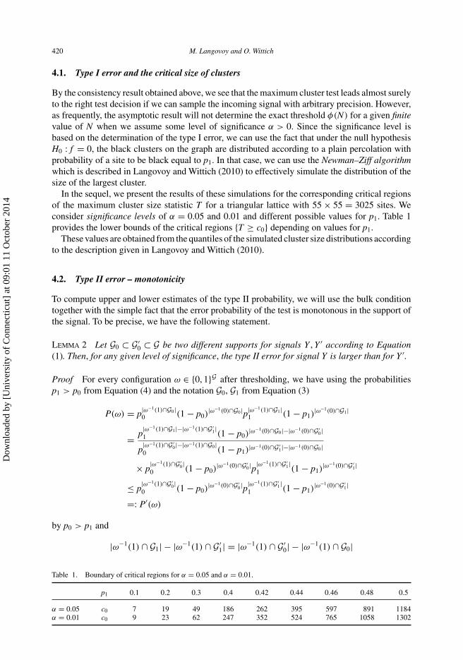
4.1. Type I error and the critical size of clusters

By the consistency result obtained above, we see that the maximum cluster test leads almost surelyto the right test decision if we can sample the incoming signal with arbitrary precision. However,as frequently, the asymptotic result will not determine the exact threshold φ(N) for a given finitevalue of N when we assume some level of significance α > 0. Since the significance level isbased on the determination of the type I error, we can use the fact that under the null hypothesisH0 : f = 0, the black clusters on the graph are distributed according to a plain percolation withprobability of a site to be black equal to p1. In that case, we can use the Newman–Ziff algorithmwhich is described in Langovoy and Wittich (2010) to effectively simulate the distribution of thesize of the largest cluster.

In the sequel, we present the results of these simulations for the corresponding critical regionsof the maximum cluster size statistic T for a triangular lattice with 55 × 55 = 3025 sites. Weconsider significance levels of α = 0.05 and 0.01 and different possible values for p1. Table 1provides the lower bounds of the critical regions {T ≥ c0} depending on values for p1.

These values are obtained from the quantiles of the simulated cluster size distributions accordingto the description given in Langovoy and Wittich (2010).

4.2. Type II error – monotonicity

To compute upper and lower estimates of the type II probability, we will use the bulk conditiontogether with the simple fact that the error probability of the test is monotonous in the support ofthe signal. To be precise, we have the following statement.

Lemma 2 Let G0 ⊂ G ′0 ⊂ G be two different supports for signals Y , Y ′ according to Equation

(1). Then, for any given level of significance, the type II error for signal Y is larger than for Y ′.

Proof For every configuration ω ∈ {0, 1}G after thresholding, we have using the probabilitiesp1 > p0 from Equation (4) and the notation G0, G1 from Equation (3)

P(ω) = p|ω−1(1)∩G0|0 (1 − p0)

|ω−1(0)∩G0|p|ω−1(1)∩G1|1 (1 − p1)

|ω−1(0)∩G1|

= p|ω−1(1)∩G1|−|ω−1(1)∩G′

1|1 (1 − p0)

|ω−1(0)∩G0|−|ω−1(0)∩G′0|

p|ω−1(1)∩G′

0|−|ω−1(1)∩G0|0 (1 − p1)

|ω−1(0)∩G′1|−|ω−1(0)∩G0|

× p|ω−1(1)∩G′

0|0 (1 − p0)

|ω−1(0)∩G′0|p|ω−1(1)∩G′

1|1 (1 − p1)

|ω−1(0)∩G′1|

≤ p|ω−1(1)∩G′

0|0 (1 − p0)

|ω−1(0)∩G′0|p|ω−1(1)∩G′

1|1 (1 − p1)

|ω−1(0)∩G′1|

=: P′(ω)

by p0 > p1 and

|ω−1(1) ∩ G1| − |ω−1(1) ∩ G ′1| = |ω−1(1) ∩ G ′

0| − |ω−1(1) ∩ G0|

Table 1. Boundary of critical regions for α = 0.05 and α = 0.01.

p1 0.1 0.2 0.3 0.4 0.42 0.44 0.46 0.48 0.5

α = 0.05 c0 7 19 49 186 262 395 597 891 1184α = 0.01 c0 9 23 62 247 352 524 765 1058 1302

Dow

nloa

ded

by [

Uni

vers

ity o

f C

onne

ctic

ut]

at 0

9:01

11

Oct

ober

201

4


and where P denotes the probability of the configuration associated to Y and P′ the probabilityassociated to Y ′. That implies for the probability that the that the signal is not detected P(T <

n0) ≥ P′(T < n0) , where n0 is a cluster size that is determined on the basis of the null hypothesisand the level of significance alone and does not therefore depend on the signal. That implies thestatement. �

Thus, under the bulk condition, we obtain a conservative upper estimate for the type II error,if we simulate the type II error for the square contained in the support of the signal and a lowerestimate if we compute it for a square containing the support. In the latter case, we will considerhere the best case scenario of a signal that is supported by all of G.

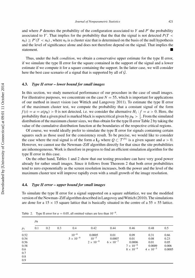
4.3. Type II error – lower bound for small images

In this section, we study numerical performance of our procedure in the case of small images.For illustrative purposes, we concentrate on the case N = 55, which is important for applicationsof our method in insect vision (see Wittich and Langovoy 2011). To estimate the type II errorof the maximum cluster test, we compute the probability that a constant signal of the formf (s) = a = a(pB) > 0 is not detected, i.e. we consider the alternative H1 : f = a > 0. Here, theprobability that a given pixel is marked black is supercritical given by pB > 1

2 . From the simulateddistribution of the maximum cluster sizes, we thus obtain for the type II error Table 2 by taking thevalue of the cumulative distribution function at the boundaries of the respective critical regions.

Of course, we would ideally prefer to simulate the type II error for signals containing certainsquares such as those used for the consistency result. To be precise, we would like to considerthe case where the real signal is of the form a 1Q where Q ⊂ T (N) is a given square and a > 0.However, we cannot use the Newman–Ziff algorithm directly for that since the site probabilitiesare inhomogeneous. Work is therefore in progress to find an efficient simulation algorithm for thetype II error in this case.

On the other hand, Tables 1 and 2 show that our testing procedure can have very good poweralready for rather small images. Since it follows from Theorem 2 that both error probabilitiestend to zero exponentially as the screen resolution increases, both the power and the level of themaximum cluster test will improve rapidly even with a small growth of the image resolution.

4.4. Type II error – upper bound for small images

To simulate the type II error for a signal supported on a square sublattice, we use the modifiedversion of the Newman–Ziff algorithm described in Langovoy andWittich (2010). The simulationsare done for a 15 × 15 square lattice that is basically situated in the centre of a 55 × 55 lattice.

Table 2. Type II error for α = 0.05, all omitted values are less than 10−9.

pB

p1 0.1 0.2 0.3 0.4 0.42 0.44 0.46 0.48 0.5

0.52 10−6 0.0005 0.01 0.09 0.31 0.660.54 5 × 10−9 10−5 0.0007 0.01 0.08 0.230.56 2 × 10−9 6 × 10−7 0.0006 0.01 0.050.58 7 × 10−6 0.0009 0.0060.6 8 × 10−9 4 × 10−5 0.00050.70.80.9

Dow

nloa

ded

by [

Uni

vers

ity o

f C

onne

ctic

ut]

at 0

9:01

11

Oct

ober

201

4


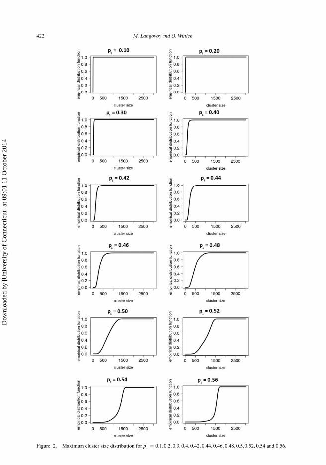
Figure 2. Maximum cluster size distribution for p1 = 0.1, 0.2, 0.3, 0.4, 0.42, 0.44, 0.46, 0.48, 0.5, 0.52, 0.54 and 0.56.

Dow

nloa

ded

by [

Uni

vers

ity o

f C

onne

ctic

ut]

at 0

9:01

11

Oct

ober

201

4


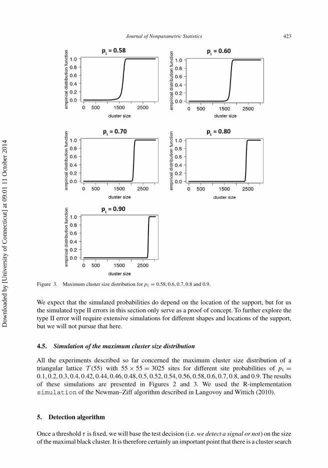
Figure 3. Maximum cluster size distribution for p1 = 0.58, 0.6, 0.7, 0.8 and 0.9.

We expect that the simulated probabilities do depend on the location of the support, but for usthe simulated type II errors in this section only serve as a proof of concept. To further explore thetype II error will require extensive simulations for different shapes and locations of the support,but we will not pursue that here.

4.5. Simulation of the maximum cluster size distribution

All the experiments described so far concerned the maximum cluster size distribution of atriangular lattice T (55) with 55 × 55 = 3025 sites for different site probabilities of p1 =0.1, 0.2, 0.3, 0.4, 0.42, 0.44, 0.46, 0.48, 0.5, 0.52, 0.54, 0.56, 0.58, 0.6, 0.7, 0.8, and 0.9. The resultsof these simulations are presented in Figures 2 and 3. We used the R-implementationsimulation of the Newman–Ziff algorithm described in Langovoy and Wittich (2010).

5. Detection algorithm

Once a threshold τ is fixed, we will base the test decision (i.e. we detect a signal or not) on the sizeof the maximal black cluster. It is therefore certainly an important point that there is a cluster search

Dow

nloa

ded

by [

Uni

vers

ity o

f C

onne

ctic

ut]

at 0

9:01

11

Oct

ober

201

4


algorithm, the Depth-First Search algorithm from Tarjan (1972), which is explained in details andimplemented in R in Langovoy and Wittich (2010), which is quite effective. That means, it islinear in the number of pixels. This is stated below. Please note that the R-implementation israther slow compared with implementations in Python or C.

We now describe the detection algorithm and state the complexity result. The algorithm consistsof the following steps:

(1) Perform a τ -thresholding of the noisy picture Y .(2) Run a Depth-First Search algorithm on the graph of the thresholded signal until either a black

cluster of size |C| ≥ c0 is found, or all black clusters are found.(3) If a black cluster of size |C| ≥ c0 was found, report that a signal was detected, otherwise do

not reject H0.

The complexity result follows now from the linear complexity of Tarjan’s algorithm (see Tarjan1972) and is given by the following statement.

Theorem 3 The algorithm terminates in O(N2) steps, i.e. it is linear in the number of pixels.

Proof See Langovoy and Wittich (2009, Theorem 1). �

Acknowledgements

The authors would like to thank Laurie Davies and Remco van der Hofstad for helpful discussions, and the AssociateEditor and the two referees for valuable suggestions that helped to greatly improve the presentation of the paper.

References

Arias-Castro, E., Donoho, D.L., and Huo, X. (2005), ‘Near-Optimal Detection of Geometric Objects by Fast MultiscaleMethods’, IEEE Transactions on Information Theory, 51(7), 2402–2425. ISSN 0018-9448.

Arias-Castro, E., and Grimmett, G. (2012), ‘Cluster Detection in Networks using Percolation’, Bernoulli.http://arxiv.org/abs/1104.0338.

Davies, P.L., Langovoy, M., and Wittich, O. (2010), ‘Randomized Algorithms for Statistical Image Analysis Based onPercolation Theory’, submitted for publication.

Fortuin, C.M., Kasteleyn, P.W., and Ginibre, J. (1971), ‘Correlation Inequalities on Some Partially Ordered Sets’,Communications in Mathematical Physics, 22, 89–103. ISSN 0010-3616.

Grimmett, G.R. (1985), ‘The Largest Components in a Random Lattice’, Studia Scientiarum Mathematicarum Hungarica,20, 325–331. ISSN 0081-6906.

Grimmett, G. (1999), Percolation, Grundlehren der Mathematischen Wissenschaften [Fundamental Principles ofMathematical Sciences] (Vol. 321, 2nd ed.), Berlin: Springer-Verlag. ISBN 3-540-64902-6.

Huo, X., and Ni, X. (2009), ‘Detectability of Convex-Shaped Objects in Digital Images, Its Fundamental Limit andMultiscale Analysis’, Statistica Sinica, 19(4), 1439–1462. ISSN 1017-0405.

Kesten, H. (1982), Percolation Theory for Mathematicians, Progress in Probability and Statistics (Vol. 2), Boston, MA:Birkhäuser. ISBN 3-7643-3107-0.

Langovoy, M., Habeck, M., and Schoelkopf, B. (2011), ‘Spatial Statistics, ImageAnalysis and Percolation Theory’, in JSMProceedings. Time Series and Network Section, Alexandria, VA: American Statistical Association, pp. 5571–5581.

Langovoy, M., and Wittich, O. (2009), ‘Detection of Objects in Noisy Images and Site Percolation on Square Lattices’,EURANDOM Report No. 2009-035, Eindhoven: EURANDOM.

Langovoy, M., and Wittich, O. (2010), ‘Computationally Efficient Algorithms for Statistical Image Processing.Implementation in R’, EURANDOM Report No. 2010-053, Eindhoven: EURANDOM.

Negri, M., Gamba, P., Lisini, G., and Tupin, F. (2006), ‘Junction-Aware Extraction and Regularization of UrbanRoad Networks in High-Resolution Sar Images’, IEEE Transactions on Geoscience and Remote Sensing, 44(10),2962–2971. ISSN 0196-2892. doi: 10.1109/TGRS.2006.877289.

Ricci-Vitiani, L., Lombardi, D.G., Pilozzi, E., Biffoni, M., Todaro, M., Peschle, C., and De Maria, R. (2007), ‘Identificationand Expansion of Human Colon-Cancer-Initiating Cells’, Nature, 445(7123), 111–115. ISSN 0028-0836.

Sinha, S.K., and Fieguth, P.W. (2006), ‘Automated Detection of Cracks in Buried Concrete Pipe Images’, Automation inConstruction, 15(1), 58–72. ISSN 0926-5805. doi: 10.1016/j.autcon.2005.02.006.

Tarjan, R. (1972), ‘Depth-First Search and Linear Graph Algorithms’, SIAM Journal on Computing, 1(2), 146–160. ISSN0097-5397.

Dow

nloa

ded

by [

Uni

vers

ity o

f C

onne

ctic

ut]

at 0

9:01

11

Oct

ober

201

4

http://arxiv.org/abs/1104.0338


Wittich, O., and Langovoy, M.A. (2011), ‘InsectVision –A Different ImageAnalysis Paradigm’, submitted for publication.Zeil, J. (1983), ‘Sexual Dimorphism in The Visual System of Flies: The Compound Eyes and Neural Superposition

in Bibionidae (Diptera)’, Journal of Comparative Physiology A: Neuroethology, Sensory, Neural, and BehavioralPhysiology, 150(3), 379–393.

Appendix

We will shortly explain how to obtain an asymptotic expression of the binomial sum in the proof of Proposition 5.

Lemma A.1 For |x| < 1, 1 ≤ n ∈ N, we have

|(1 + x)n − 1 − nx| ≤ n(n − 1)

2|x|2(1 + |x|)n−2. (A1)

Proof We have

|(1 + x)n − 1 − nx| ≤n∑

k=2

(nk

)|x|k

= n(n − 1)

2|x|2

n∑k=2

(nk

)(

n2

) |x|k−2

≤ n(n − 1)

2|x|2

n−2∑k=0

(n − 2

k

)|x|k

= n(n − 1)

2|x|2(1 + |x|)n−2.

�

Lemma A.2 Let zN = e−λf (N) and f (N) = C log(N2) = 2C log(N), where λ > 0 and λC > 1. Then, as N tends toinfinity, we have

1 − (1 − zN )N2 = N2(1−Cλ) + O(N4(1−Cλ)). (A2)

Proof By inequality (A1)

|(1 − zN )N2 − 1 + N2zN | ≤ N2(N2 − 1)

2z2

N (1 + |zN |)N2−2.

By Cλ > 1, we obtain

limN→∞(1 + |zN |)N2−2 = lim

N→∞

(1 + 1

N2Cλ

)N2

= 1.

Thus, for N > N0 large enough, there are constants K∗ > K > 1 such that

|(1 − zN )N2 − 1 + N2zN | ≤ KN2(N2 − 1)

2z2

N ≤ K∗N4(1−Cλ).

Together withN2zN = N2(1−Cλ),

that proves the assertion. �

Proof of Proposition 5 Let s ∈ T (N) and C(s) the (possibly empty) largest connected cluster of occupied sites in T thatcontains s. The event {|C(s)| < n} is obviously decreasing for all s ∈ T (N). That implies by FKG inequality

P

(max

s∈T (N)|C(s)| < n

)= P(∩s∈T (N) {|C(s)| < n})

≥∏

s∈T (N)

P(|C(s)| < n).

By Equation (8) and translation invariance on the infinite lattice, we thus obtain

P

(max

s∈T (N)|C(s)| < n

)≥ (1 − e−λ(p1)n)N2

.

Hence,P(F(N)(n)) ≤ 1 − (1 − e−λ(p1)n)N2

.Let now n = 2C log N = φ(N) with Cλ(p1) > 1. Then, by Equation (A2), we obtain

P(F(N)(φ(N))) = N−2(Cλ(p1)−1) + O(N−4(Cλ(p1)−1)). �

Dow

nloa

ded

by [

Uni

vers

ity o

f C

onne

ctic

ut]

at 0

9:01

11

Oct

ober

201

4


Proof of Proposition 7 Let s ∈ T (N) and C(s) the (possibly empty) largest connected cluster of occupied sites in T thatcontains s. The event {|C(s)| < n} is obviously decreasing for all s ∈ T (N). That implies by FKG inequality

P

(max

s∈T (N)|C(s)| < n

)= P(∩s∈T (N) {|C(s)| < n})

≥∏

s∈T (N)

P(|C(s)| < n).

By Equation (8) and translation invariance on the infinite lattice, we thus obtain

P

(max

s∈T (N)|C(s)| < n

)≥ (1 − e−λ(p1)n)N2

.

Hence,P(F(N)(n)) ≤ 1 − (1 − e−λ(p1)n)N2

.Let now n ≥ 2C log N with Cλ(p1) > 1. Then, by essentially the same calculation as for Equation (A1), we obtain

P(F(N)(n)) ≤ N2e−λ(p1)n(1 + e−λ(p1)n)N2−1

≤ N2(1 + N−2Cλ(p1))N2−1e−λ(p1)n.

Now, n ≥ C log N2 and thus log N2 ≤ n/C. That implies by Cλ > 1 and

limN→∞(1 + N−2Cλ(p1))N2−1 = 1.

This implies that, for N large enough, we have

(1 + N−2Cλ(p1))N2−1 ≤ eκn.

If we take K (N) := λ(p1) − κ − C−1 > 0, we obtain

log N2 + κ − λ(p1)n ≤(

1

C+ κ − λ(p1)

)n = −K (N)n,

which implies the proposition. �

Dow

nloa

ded

by [

Uni

vers

ity o

f C

onne

ctic

ut]

at 0

9:01

11

Oct

ober

201

4

robust nonparametric detection of objects in noisy images

Documents