robust polynomial controller design
TRANSCRIPT

ROBUST POLYNOMIAL CONTROLLER DESIGN
A Thesis submitted for the degree of Doctor of Philosophy
by
Kevin Well stead
September 1991
BruneI University
Control Engineering Centre
Department of Electrical Engineering and Electronics
Uxbridge
Middlesex
UB83PH
U.K.

MEMORANDUM
Statement of Originality
The accompanying thesis is based on work carried out by the author at BruneI University between
October 1988 and September 1991.
All work and ideas in this thesis are original, unless otherwise acknowledged in the text or by
references. The work has not been submitted for another Degree in this university, nor for the
award of a Degree or Diploma at any other Institution.
The main contribution of this work is the proposal of an alternative approach to the design of
robust polynomial control systems. It utilises state space techniques by transforming the system
to state space form, performing the design and transforming the resulting controller back to
polynomial form.
During the period of this research two particular aspects have been reported in the technical
literature. The references for these articles are
1) 'On Finding Polynomial Controllers with Reduced Pole Sensitivity using
State Space Methods'
Wellstead, K.D. and Daley, S.
lEE International Conference, Control'91, Edinburgh, U.K., vI, pp 677-681
lEE, London, U.K. (Conf Publ No. 332)
2) 'A Parametric Design Approach for Observer Based Fault Detection'
Wang, H., Daley, S. and Wellstead, K.D.
Eigth International Conference on Systems Engineering, Coventry, U.K., pp 248-255
ISBN 0905949 102
11

ROBUST POL YNO~lIAL CONTROLLER DESIGN
Kevin Wellstead
1991
BruneI University, Control Engineering Centre, Department of Electrical Engineering and Electronics,
Uxbridge, Middlesex, UB8 3PH. U.K.
ABSTRACT
The work presented in this thesis was motivated by the desire to establish an alternative
approach to the design of robust polynomial controllers. The procedure of pole-placement forms
the basis of the design and for polynomial systems this generally involves the solution of a
diophantine equation. This equation has many possible solutions which leads directly to the idea
of determining the most appropriate solution for improved performance robustness.
A thorough review of many of the aspects of the diophantine equation is presented, which
helps to gain an understanding of this extremely important equation. A basic investigation into
selecting a more robust solution is carried out but it is shown that, in the polynomial framework,
it is difficult to relate decisions in the design procedure to the effect on performance robustness.
This leads to the approach of using a state space based design and transforming the resulting
output feedback controller to polynomial form.
The state space design is centred around parametric output feedback which explicitly
represents a set of possible feedback controllers in terms of arbitrary free parameters. The aim
is then to select these free parameters such that the closed-loop system has improved performance
robustness. Two parametric methods are considered and compared, one being well established
and the other a recently proposed scheme. Although the well established method performs slightly
better for general systems it is shown to fail when applied to this type of problem.
For performance robustness, the shape of the transient response in the presence of model
uncertainty is of interest. It is well known that the eigenvalues and eigenvectors play an important
role in determining the transient behaviour and as such the sensitivities of these factors to model
uncertainty forms the basis on which the free parameters are selected. Numerical optimisation
is used to select the free parameters such that the sensitivities are at a minimum.
It is shown both in a simple example and in a more realistic application that a significant
improvement in the transient behaviour in the presence of model uncertainty can be achieved
using the proposed design procedure.
III

TABLE OF C():\TEl\TS
Chapter One - INTRODUCTION
1.1 Historical Background
1.2 Preliminaries
1.3 Definition of the Problem
1.4 Pole-Placement Design for Polynomial Systems
1.5 Objective of the Thesis
1.6 Outline of the Thesis
References
Chapter Two - THE DIOPHANTINE EQUATION
2.1 Introduction
2.2 Solution via Polynomial Methods
2.3 Solution via Matrix Methods
2.4 Problems Associated with Finding a Solution
2.5 Obtaining a More Robust Solution
2.5.1 The Effect of Parameter Perturbations
2.5.2 Matrix and Vector Norms
2.5.3 Selecting the Order of the Controller Polynomials
2.5.4 Simulation Results
2.6 Conclusions
References
Chapter Three - STATE SPACE DESIGN FOR POLYNOMIAL SYSTEl\1S
3.1 Introduction
3.2 Modal Decomposition
3.3 The Link between Polynomial and State Space Representations
IV
12
13
15
16
20
21
23
26
28
30
31
35
36
38
39
41
43
58
60
61
63

3.4 State Space Design
3.4.1 The Parametric Output Feedback Method of Fahmy and O'Reilly
3.4.2 The Parametric Output Feedback Method of Daley
3.4.3 Examples used for the Comparison of the Methods
3.4.4 Results for the Method of Fahmy and O'Reilly
3.4.5 Results for the Method of Daley
3.4.6 Discussion of the Results
3.5 Summary
References
Chapter Four - SELECTING A ROBUST CONTROLLER
4.1 Introduction
4.2 Cost Functions
4.2.1 Eigenvalue Differential Cost Function
4.2.2 Eigenstructure Differential Cost Function
4.2.3 Transient Response Differential Cost Function
4.2.4 Conditioning Cost Function
4.3 Optimisation Techniques
4.3.1 Introduction and Terminology
4.3.2 Classification of the Problem
4.3.3 Common Optimisation Methods
4.4 Summary
References
Chapter Five - IMPLEMENTATION AND APPLICATION OF THE
ROBUST DESIGN PROCEDURE
5.1 Introduction
5.2 Implementation of the Robust Design Procedure
5.2.1 The Link Between PRO-MA TI.AB and FORTRAN 77
5.2.2 Calculation of the Null Space of a Matrix in FORTRAN 77
5.2.3 Calculation of an Accurate Inverse of a Matrix in FORTRAN 77
v
66
68
73
76
80
82
85
87
89
91
93
94
96
98
100
102
102
106
108
109
110
112
113
114
117
118

,", I r'
5.3 Application of the Robust Design Procedure
5.3.1 Definition of the System and Preliminary Work
5.3.2 Problems Associated with the Parametric Method of Fahmy and O'Reilly
5.3.3 Determining the Number of Free Parameters
5.3.4 Selecting the Optimisation Routine
5.3.5 Layout of the Results
5.3.6 Results for the Eigenvalue Differential Cost Function
5.3.7 Results for the Eigenstructurc Differential Cost Function
5.3.8 Results for the Transient Response Differential Cost Function
5.3.9 Results for the Conditioning Cost Function
5.4 Summary and Discussion of the Results
References
Chapter Six - APPLICATION TO A HYDRAULIC RIG
6.1 Introduction
6.2 Nonlinear Simulation and Model Identification
6.3 Controller Design
6.3.1 Minimum Order Polynomial Controller Design
6.3.2 Robust Polynomial Controller Design
6.4 Discussion of the Results and Conclusions
References
Chapter Seven - CONCLUSIONS
7.1 Summary and General Discussion
7.3 Problems and Future Work
7.4 Concluding Remarks
References
vi
120
120
123
128
130
130
133
139
141
142
143
151
152
153
157
157
158
164
172
173
176
178
179

Appendix A - ALGORITH;\1S FOR THE POLY:\O\lIAL SOLLTIO:\
OF THE DIOPHA:\TI:\E EQCATIO:\
A.l Introduction
A.2 Division of Polynomials Algorithm
A.3 Extended Euclidean Algorithm
References
Appendix B - PROGRAMS FOR THE ROBUST POLYNOMIAL
CONTROLLER DESIGN
B.l Pre-Optimisation Programs - PRO-MATLAB
B.2 Optimisation Programs - FORTRAN 77
B.3 Post-Optimisation Programs - PRO-MATLAB
Appendix C - DETAILS OF THE NAG LIBRARY ROUTINES
C.1 Accurate Inverse of a Real Matrix
C.2 Calculation of the Null Space of a Matrix
C.3 Non-Linear Optimisation
References
Appendix D - ACSL SIMULATION PROGRAMS
D.l Open-Loop Simulation
D.2 Closed-Loop Simulation
NOMENCLATURE AND SYMB()LS
VII
180
180
181
182
183
186
198
200
203
204
206
207
208
210

TABLE ()F TABLES
Table 5.1 Pole Positions for the Perturbed Closed-Loop System with the
Minimum Order Controller 121
Table 6.1 IV Estimation Results 155
Table 6.2 Pole Positions for the Perturbed Closed-Loop System with the
Minimum Order Controller 158
Table 6.3 Ratio of the Changes in the Open-Loop Polynomial Coefficients 159
Table 6.4 Eigenvalue Sensitivities for the Robust Ps design 160
Table 6.5 Pole Positions for the Perturbed Closed-Loop System with the
Robust Ps Controller 161
Table 6.6 Eigenvalue Sensitivities for the Robust P p design 162
Table 6.7 Pole Positions for Perturbed Closed-Loop System with the
Robust P p Controller 162
Table 6.8 Eigenvalue Sensitivities for the Robust Ps and P p design 163
Table 6.9 Pole Positions for Perturbed Closed-Loop System with the
Robust Ps and P p Controller 164
\' III
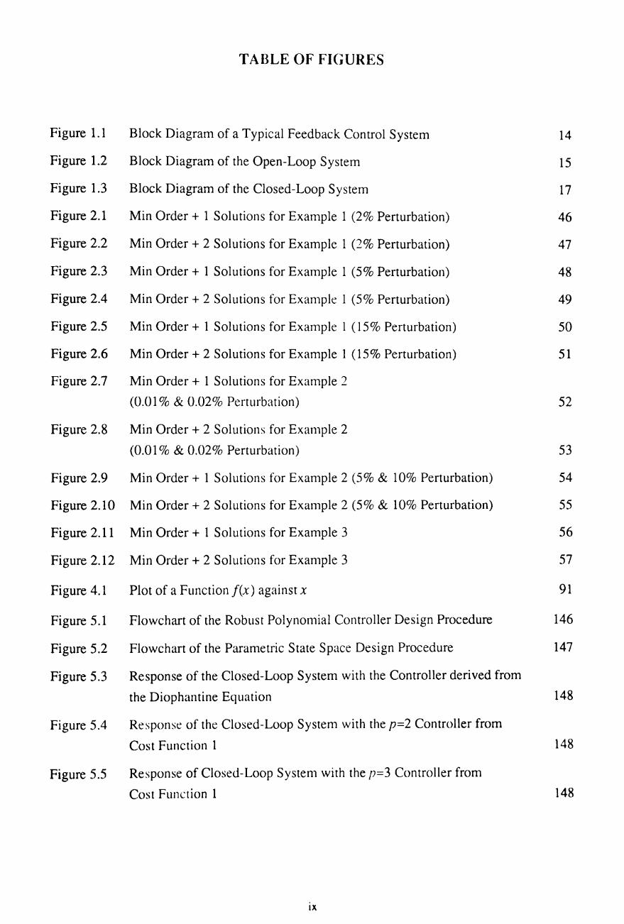
TABLE OF FIGURES
Figure 1.1 Block Diagram of a Typical Feedback Control System 14
Figure 1.2 Block Diagram of the Open-Loop System 15
Figure 1.3 Block Diagram of the Closed-Loop System 17
Figure 2.1 Min Order + 1 Solutions for Example 1 (2% Perturbation) 46
Figure 2.2 Min Order + 2 Solutions for Example 1 (2% Perturbation) 47
Figure 2.3 Min Order + 1 Solutions for Example 1 (5% Perturbation) 48
Figure 2.4 Min Order + 2 Solutions for Example 1 (5% Perturbation) 49
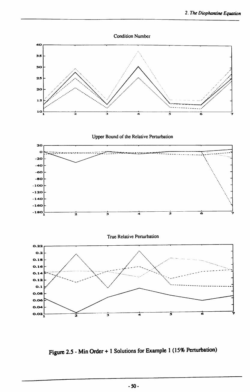
Figure 2.5 Min Order + 1 Solutions for Example 1 (15% Perturbation) 50
Figure 2.6 Min Order + 2 Solutions for Example 1 (15% Perturbation) 51
Figure 2.7 Min Order + 1 Solutions for Example 2
(0.01 % & 0.02% Perturbation) 52
Figure 2.8 Ivlin Order + 2 Solutions for Example 2
(0.01 % & 0.02% Perturbation) 53
Figure 2.9 Min Order + 1 Solutions for Example 2 (5% & 10% Perturbation) 54
Figure 2.10 Min Order + 2 Solutions for Example 2 (5% & 10% Perturbation) 55
Figure 2.11 Min Order + 1 Solutions for Example 3 56
Figure 2.12 Min Order + 2 Solutions for Example 3 57
Figure 4.1 Plot of a Function I(x) against x 91
Figure 5.1 Flowchart of the Robust Polynomial Controller Design Procedure 146
Figure 5.2 Flowchart of the Parametric State Space Design Procedure 147
Figure 5.3 Response of the Closed-Loop System with the Controller derived from
the Diophantine Equation 148
Figure 5.4 Response of the Closed-Loop System with the p=2 Controller from
Cost Function 1 148
Figure 5.5 Response of Closed-Loop System with the p=3 Controller from
Cost Function 1 148
IX

Figure 5.6 Response of Closed-Loop System with the p=4 Controller from
Cost Function 1 149
Figure 5.7 Response of Closed-Loop System with the p=2 Controller from
Cost Function 2 149
Figure 5.8 Response of Closed-Loop System with the p=3 Controller from
Cost Function 2 149
Figure 5.9 Response of Closed-Loop System with the p=3 Controller from
Cost Function 3 150
Figure 5.10 Response of Closed-Loop System with the p=2 Controller from
Cost Function 4 150
Figure 5.11 Response of Closed-Loop System with the p=3 Controller from
Cost Function 4 150
Figure 6.1 Schematic of the Hydraulic Circuit of the Rig 166
Figure 6.2 Response of the Open-Loop System 167
Figure 6.3 Response of the Closed-Loop System with the Minimum Order
Controller 168
Figure 6.4 Response of the Closed-Loop System with the Robust Ps Controller 169
Figure 6.5 Response of the Closed-Loop System with the Robust Pp Controller 170
Figure 6.6 Response of the Closed-Loop System with the Robust Ps and P p
Controller 171
x

To my Mother and Father
ACKNOWLEDGEMENTS
I would like to thank my supervisor, Steve Daley, for all his help and encouragement over
the three years of research culminating in this thesis. His support has been invaluable to the
successful completion of this work.
Thanks must also go to John Marsh for his help with a number of theoretical aspects
particularly in the field of linear algebra, and also to Tom Owens whose comments have helped
tremendously both in carrying out the actual research and in the production of this thesis.
My colleague Hong Wang deserves thanks for a number of enlightening and fruitful dis
cussions on many aspects of control systems design, and for his assistance in a number of areas
I would also like to thank Bruce Baxter.
In research probably the most baffling problems are those associated with the equipment
being used, particularly these days in the field of computing! Such problems can be frustrating
and time consuming to deal with. To this end I am extremely grateful to John Philips for all his
patience and help in solving the never ending list of problems I presented him with, and for doing
so with good humour.
For their help and advice regarding many aspects of the university'S computing facilities
I would like to thank all those in the Computer Centre and in particular Raghbir Pank for his
assistance with the NAG Fortran Library.
Dilip Dholiwar and the GEC Alsthom Engineering Research Centre also deserve thanks
for supplying the data for the simulation of the hydraulic test rig.
This work was funded by the U.K. Science and Engineering Research Council.
,\1

CHAPTER 1
INTRODUCTION
1.1 Historical Background
The problem of designing accurate control systems in the presence of significant plant
uncertainties is classical, Dorato (1987). This problem has been dealt with as far back as the
1920's when Black (1927) proposed using feedback with large loop gains to overcome the
problem of significant variations in vacuum tube characteristics in the design of a vacuum tube
amplifier. Dorato (1987) details the development of robust control theory from this early proposal
and the classical work of Nyquist (1932) and Bode (1945) through to the late 1980's.
In the 1960's and 1970's much attention was focused on the state variable approach and
in particular the linear quadratic Gaussian (LQG) method for optimal control. Kalman (1964)
and Safonov and Athans (1977) showed that the optimal LQG state feedback control laws had
some very strong robustness properties with infinite gain margins and 60-deg phase margins.
However, in practice it is often necessary to employ Kalman filter theory to obtain an optimal
estimate of the state vector which is then taken as an exact measurement in the LQG design.
Doyle (1978) showed that when an estimate of the state vector is used, the design can exhibit
arbitrarily poor stability margins and the robustness properties vanish.
LQGIL TR (linear quadratic Guassian/loop transfer recovery), Doyle and Stein (1979,
1981), provides a means of overcoming these problems by designing the Kalman filter such that
the full state feedback properties are 'recovered'. One drawback is the inability of the method
to deal with non-minimum phase systems as the procedure involves cancelling some of the filter
poles with plant zeros.
Of particular importance to the shaping of robust methods today are three major discoveries
in the late 1970's and early 1980's (Morari and Zafiriou, 1989). Youla et at (1976) showed that
it is possible to parameterise all stabilising controllers for a particular system in a very effective
manner, which guarantees that the resulting feedback controller automatically yields a closed
loop stable system. This effectively gives rise to a set of possible controllers which greatly
simplifies the search for a more robust one. Zames (1981) postulated that measuring performance
in terms of the oo-norm rather than the traditional2-noml might be closer to practical needs. This
helped to establish the H _ optimal control approach to robust controller design. The work of
Doyle in a number of papers in the early 1980's (Doyle and Stein, 1981; Doyle and Wall, 1982:
Doyle, 1982) is quite important in the development of robust control theory. He argued that
model uncertainty is often described very effectively in terms of norm-bounded perturbations.
- 12 -

1. I mrodUCIWn
He developed the structured singular value approach for testing 'robust stability' (i.e., stability
in the presence of model uncertainty) and 'robust performance' (i.e., performance in the presence
of model uncertainty), and is probably the primary motivation for the modern eo-norm objective.
Other techniques for robust design include representing the model uncertainty stochasti
cally as in Wonham (1967) and the game theoretic or minimax approach which basically
represents the uncertainty as a factor that maximises a performance measure which is being
minimised by the control variable (for example Ragade and Sarma, 1967; Bertsekas and Rhodes,
1973). The minimax approach can, however, become quite complicated for relatively simple
design problems. It is also worth mentioning quantitative feedback theory (Horowitz, 1979,
1982; Horowitz and Sidi, 1980) which is based on loop gain shaping and the use of templates
to represent the model uncertainty, each of which contains the set of possible plant transfer
function values at a particular frequency. Other authors (for example Gourishankar and Ramar,
1976; Owens and O'Reilly, 1989) have suggested that the design be based on the sensitivities
of the eigenvalues and eigenvectors. The conditioning of the matrix of eigenvectors has also
been suggested as a good basis on which to design robust controllers (Kautsky et ai, 1985; Byers
and Nash, 1989). Further information on these methods and other alternative approaches to the
robust control problem can be found in Dorato (1987), Maciejowski (1989) and Morari and
Zafiriou (1989).
A discussion of a number of preliminary points regarding some basic definitions in the
general robust control problem is presented next, followed by more specific information on the
type of system being considered and the problem of interest. This naturally leads to a discussion
of the objectives of this work and an outline of the thesis.
1.2 Preliminaries
Robust design attempts to take account of uncertainty in the model and disturbances on
the system. Model uncertainty arises due to the difference between the real plant and the model
being used for the design of the controller. When modelling a system it is often necessary to
make certain assumptions such that the problem can be simply defined and a model easily
obtained. Examples of such assumptions are linearity, the order of the model, the time delay,
noise characteristics and the time invariance of parameters. The errors introduced by such
assumptions can give rise to model uncertainty.
Model uncertainty can generally be split into two categories, unstructured and structured.
To help understand the difference between the two, consider the typical feedback control system
shown in figure 1.1 where P is the plant, C is the controller, w (t) is the demand signal, e (t) is
the error, u (t) is the input and y(t) the output.
------------- ~ ~~--~-
- 13 -

1. I mroduction
e(t) u(t) c p yet) ~-
Figure l.1 - Block Diagram of a Typical Feedback Control System
P can be expressed as
P=M+~ (1.1)
where M represents the derived model of the plant and ~ the modelling error or uncertainty
due to the violation of certain assumptions as outlined above.
An unstructured description of the model uncertainty essentially bounds the magnitude of
possible perturbations, i.e.
II ~II ~ Il <-too (1.2)
but does not trace the origins of the perturbations to specific elements of the plant. A structured
description can be represented as
~=K£ (1.3)
and attempts to specify some information, using K, regarding which elements of the plant are
subject to perturbations. £ represents the unknown magnitude of the perturbations.
Clearly the unstructured approach may lead to controller designs which are unnecessarily
conservative as it can include perturbations which do not actually occur in the plant. A structured
approach on the other hand has the drawback that it does not deal with perturbations that affect
the order of the plant (Maciejowski, 1989).
- 14 -

1. /nlrodJl.ction
The robustness problem itself can primarily be split into two types, robust stability and
robust performance. The stability problem is concerned with ensuring that the closed-loop system
remains stable in the face of model uncertainty, whereas robust performance is concerned with
how the closed-loop system behaves subject to model uncertainty.
1.3 Definition of the Problem
This work is concerned with discrete single-input single-output (SISO) systems in
input-output (or polynomial) form. The open-loop system is as shown in figure 1.2
e(t) C A
u(t) B + Y (t) -A +
Figure 1.2 - Block Diagram of the Open-Loop System
which can be expressed as
(1.4)
where
-I -1 -2 -II. A (z )=I+az +az +···+a z
p I 2 ". (1.5)
( -I) b b -I b -2 + b -II. B p z = 0 + IZ + 2Z + . . . ". Z (1.6)
C ( -I) 1 -I -2 + -II, Z = +c z +c z + ... c z p I 2 ",
(1.7)
and Z-I can be interpreted as the backward shift operator. The signals yet), u(t) and ee,) are the
sampled system output, the control input and a white noise sequence respectively. C,(Z-l) is a
colouring polynomial for the signal e(t), used to characterise the disturbance more accurately .
• IS·

1. I mroduction
For this type of system, the problem considered is that of performance robustness. To
ensure that the problem remains tractable it is assumed that the orders of the system polynomials
Ap(Z-l) and Bp(Z-l) are fairly accurate and that information is available on which coefficients are
perturbed, thus the problem is one of structured model uncertainty. For the general polynomial
system this can be expressed as
( 1.8)
(1.9)
where aI' .. " an ,bo, .. " bn are the known nominal values of the coefficients and &21, •• " &2n , a b a
Mo, .. " Mnb are the unknown errors or variations in the coefficients, some of which may be
zero.
The concept of pole-placement for controller design has its roots in classical control theory
and the idea of placing poles in certain locations to achieve a desired closed-loop behaviour is
intuitively appealing. The methods for perfomling such a design are generally quite straight
forward and all of these points help to explain why pole-placement has become very popular in
industry for controller design. On the basis of this the approach of pole-placement is adopted as
the design procedure for this work.
Before continuing with details of the objectives of this thesis and an outline of the various
chapters, it is useful to review the pole-placement design procedure for polynomial systems.
1.4 Pole-Placement Design for Polynomial Systenls
Following Wellstead and Sanoff (1981), servo and regulatory control can be applied to
the system in (1.4) using the control law:
(1.10)
where
- 16 -

1. I nJroduclion
(1.11)
G ( -1) -1 -2 -11, P Z = go + g 1 Z + g 2Z + ... + gil Z , (1.12)
H ( -1) h h -1 h -2 h -1110 P Z = 0 + 1Z + 2Z + ... + 1110 Z (1.13)
and w (t) is the demand signal.
Note that the pole-placement design assumes the time delay, td is incorporated in B/z-1),
hence nb = fib + td where fib is the true order of Bp (Z-1). This will lead to some of the leading
coefficients of Bp (Z-1) being zero. Also, due to sampling, the time delay will always be at least
one, so bo will be equal to zero.
This gives rise to the closed-loop system as shown in figure 1.3
e(t) c A
w (t) + 1 u(t) B + Y H - - -
F A + -
(t)
G
Figure 1.3 - Block Diagram of the Closed-Loop System
which can be expressed as
(1.14)
- 17 -

J. IlIlroductWlI
HTp(Z-I) = 1 + tlZ-1 + ~Z-I + ... + tll,z -, specifies the desired closed-loop pole positions then
Fp(Z-I) and G p(Z-I) are obtained from the solution to the diophantine equation
(1.15)
where Cp(Z-I) is included on the right hand side (RHS) of the equation to minimise the variance
of the disturbance. To explain, consider the disturbance tenn
(1.16)
The variance of d(t), E[d2(t)] can be expressed as
E[d2(t)] = E[e 2(t) + c;e 2(t -1) + c;e\t - 2) + ...
. . . +c1e(t)e(t - 1) + c2e (t)e(t - 2) + ...
. . . + c1c2e(t - l)e(t - 2) + ... ] (1.17)
But as e(t) is an uncorrelated sequence
E[e(t - a)e(t - ~)] = 0 for a;t ~ (1.18)
Therefore
E[d2(t)] = E[1 + c; + c; + ... ]a! (1.19)
where cr. is the variance of e (t).
Clearly if C p(z -I) can be removed from the disturbance term, the variance will be minimised.
This can be achieved by forcing the denominator of the closed-loop system to contain Cp(Z-I)
as a factor, hence the fonn of the diophantine equation (1.15).
This gives the closed-loop system as
- 18-

1.lnlrodUClwn
(1.20)
where the denominator of the demand signal term still contains Cp(Z-I) which can be removed
using the precompensator, Hp(Z-I), by incorporating it as a factor, i.e.
(1.21 )
Essentially the precompensator term, H/(Z-I) is used to ensure that the output yet) tracks
the command input wet) in the steady state. Considering the response of the closed-loop system
to a step input, for zero steady state error
__ B=--p (_1 )_H....:....p '_(1_)--....:C p:....-(_l)_ = 1 A p ( 1 )F p ( 1 ) + B p ( 1 )G p ( 1 )
(1.22)
The form of H/(I) which ensures that this equation is satisfied is not unique. If Ap(Z-I) is
forced to contain a factor of (1 - Z-I) by cascading a digital integrator with the open-loop system,
then A/I) = 0 and hence H/(l) can be obtained from
(1.23)
and as this represents a scalar value, nh' = O. Therefore Hp(Z-I) = H/(l)C/z-l) and nh = nco
However in practice the model parameters A/z-I), Bp(Z-I) and C/z-I) are generally not
accurately known and estimates are used. Hence F/z-I) and G p(Z-I) are obtained from
(1.24)
where Ap(Z-I), B p(Z-I) and C p(Z-I) are estimates of the model parameters. Hp(Z-I) is then
calculated as above using the estimates of the model parameters.
- 19 -

1. 1 ntroduction
1.5 Objective of the Thesis
From a robustness point of view the diophantine equation is extremely interesting due to
the large number of possible solutions, all of which lead to a stabilising controller that places
the closed-loop poles in the desired locations. Particular solutions may however yield a
closed-loop system with improved robustness properties.
The robust design problem can now be stated as the determination of suitable Fp(Z-l) and
G iz-l) polynomials which satisfy the diophantine equation (1.15) and which minimise the effect
of &Zl' ... , &zIlG' Mo, ... , Mllb on the transient response of the closed-loop system.
Uncertainty in the Cp(Z-I) polynomial is not considered as it does not affect the transient
behaviour of the closed-loop system. It is incorporated, however, in the precompensator Hiz-l)
which is selected to achieve zero steady state error. The presence of uncertainty does not represent
a problem for steady state tracking if the procedure for selecting the precompensator outlined in
the previous section is used. Considering the expression for the precompensator, in the steady
state
(1.27)
and it is clear that good steady state tracking will always be maintained as Hp(l) is independent
of any uncertainty in Cp(Z-I).
Now consider how to solve this problem and obtain the robust Fp(Z-l) and Gp(Z-l) poly
nomials. Section 1.1 gave an indication of various approaches to the solution of the robust control
problem and it was noted that a major development was the Youla parameterisation which
effectively gives rise to a set of possible controllers, allowing the most robust one to be found.
Obtaining a solution to the diophantine equation represents a similar situation where there are
a set of controllers and the problem becomes one of searching for the most robust controller.
The concept of searching for a robust controller is quite natural in robust design and is
easily fonnulated in tenns of an optimisation problem. Indeed many robust techniques involve
some fonn of optimisation in the design of a suitable controller. The rapid development in
computing technology over recent years opens up the possibility of solving the optimisation
problem numerically, Maciejowski (1989).
This thesis presents an alternative approach to the solution of the robust design problem
as outlined above, based on the theme of utilising modem computing technology to conduct the
seaICh for a robust controller, in the form of a numerical optimisation problem.
·20-

J. I nJroduction
1.6 Outline of the Thesis
Chapter 2: The diophantine equation is clearly extremely important in the design of a
controller for systems in input-output form. This chapter discusses a number of the aspects of
this equation to help gain a better understanding of the robust controller design problem. There
are two main approaches to solving the equation and they are both reviewed, followed by a
discussion of various problems that may be encountered when attempting to find a solution. A
simple approach to finding a more robust controller is then developed but it is shown that the
method has a number of shortcomings, which leads directly to the idea of a state space design.
Chapter 3: The link between polynomial and state space systems is established showing
that, as would be expected, an output feedback state space design must be used. As the aim is
to use optimisation techniques to select a more robust controller, a parametric design is used
which effectively specifies a set of possible controllers. Two of the main parametric output
feedback methods are reviewed and a comparison made of their performance on some test
examples. The method which performs better is however not used as the structure of the type of
problem being considered here causes it some difficulty. This is discussed more fully when the
overall design is applied to an example in chapter 5.
Chapter 4: After determining the set of possible controllers using parametric design, the
problem becomes one of how to selec't the free parameters such that the resulting controller yields
a closed-loop system with improved performance robustness. This issue is addressed in this
chapter, which first introduces how to quantify mathematically the effect of errors in the model.
A mathematical description of the output is then obtained using modal decomposition and from
this a number of possible cost functions are derived for use with numerical optimisation algo
rithms. A general introduction into such algorithms is then given.
Chapter 5: The previous chapters develop the overall robust design technique, this chapter
applies the method to an example. With the application of the method arises questions and
problems associated with its implementation on a computer and a small discussion of some of
the most important points is given. It is then shown why one of the parametric design methods
cannot be used on the this type of problem. A comprehensive set of results is then obtained which
helps to illustrate the relative benefits of each of the proposed cost functions and the typical
improvement that can be achieved with this robust design approach.
Chapter 6: The application of the method to a more realistic problem is considered in this
chapter. Daley (1987) considered the application of self-tuning control to a hydraulic rig to help
overcome problems associated with varying supply pressure and load. From the basic physical
equations of the plant a nonlinear continuous time simulation of the rig is set up and a robust
controller designed from a model obtained using system identification techniques. It is shown
- 21 -

J.lnlroducrwn
that the robust controller performs well compared to the controller obtained from the minimum
order solution to the diophantine equation. Also the perfomlance compares favourably with that
of the self-tuning controller of Daley (1987).
Chapter 7: The conclusions drawn from the preceding chapters are presented here. The
chapter brings together and highlights both the advantages and the disadvantages of this type of
approach to designing robust controllers. There are still a number of problems with the method
and a discussion of these follows, leading onto some suggestions for future work.
- 22 -

1. IlIlrodllCtioll
REFERENCES
Bertsekas, D.P. and Rhodes,I.B. (1973)
'Sufficiently Informative Functions and the Minimax Feedback ConlIol of Uncertain Dynamic Systems' IEEE Transactions on Automatic Control, v18, n4, pp 117-124
Black, H.S. (1927)
'Stabilized Feedback Amplifiers' U.S. Patent 2,102,671
Bode, H.W. (1945)
'Network Analysis and Feedback Amplifier Design'
Van Nostrand. Wokingham. UK.
Byers, R. and Nash, S.O. (1989)
, Approaches to Robust Pole Assignment'
International Journal of Control, v49, n 1, pp 97-117
Daley, S. (1987)
'Application of a Fast Self-Tuning Control Algorithm to a Hydraulic Test Rig'
Proceedings of the Institute of Mechanical Engineers, v201, nC4, pp 285-295
Dorato, P. (1987)
, A Historical Review of Robust Control'
IEEE Control Systems Magazine, v7, n2, pp 44-47
Doyle, J.C. (1978)
'Ouaranteed Margins for LQO Regulators'
IEEE Transactions on Automatic Control, v23, n4, pp 756-757
Doyle, J.C. (1982)
, Analysis of Feedback Systems with Structured Uncertainties'
lEE Proceedings, v129, Pt D, n6, pp 242-250
Doyle, J.C. and Stein, O. (1979)
'Robustness with Observers'
IEEE Transactions on Automatic Control, v24, n8, pp 607-611
Doyle, J.C. and Stein, O. (1981)
'Multivariable Feedback Design: Concepts for a Classical/Modem Synthesis'
IEEE Transactions on Automatic Control, v26, n2, pp 4-16
Doyle, J.C. and Wall, J.E. (1982)
'Performance and Robustness Analysis for Structured Uncertainty'
Proceedings of the 21 sl IEEE Conference on Decision and Control. Orlando. Florida. U.S.A. v2, pp 629-636
IEEE. New York. U.S.A.
Gourishankar, V. and Ramar, K. (1976)
'Pole Assignment with Minimum Eigenvalue Sensitivity to Plant Parameter Variations'
IlIIernatioMI JOUTMI ofColllrol, v23, 04, pp 493-504
Horowitz, I. (1979) 'Quantitative Synthesis of Uncertain Multiple Input-Output Feedback Systems'
IlIIerfllJlionaJ JOUT"",l ofColllrol, v30, nl, pp 81-106
-23 -

Horowitz, I. (1982)
'Quantitative Feedback Theory'
lEE Proceedings, v129, Pt D, n6, pp 215-226
Horowitz, L and Sidi, M. (1980)
'Practical Design of Multivariable Feedback Systems with Large Plant Uncertainty' International Journal 0/ Systems Science, vII, pp 851-875
Kalman, R.E. (1964)
'When is a Linear Control System Optimal?'
Transactions 0/ the ASME, Ser D, Journal 0/ Basic Engineering, v86, pp 51-60
Kautsky, J., Nichols, N.K. and Van Dooren, P. (1985)
'Robust Pole Assignment in Linear State Feedback'
International Journal o/Control, v41, n5, pp 1129-1155
Maciejowski, J .M. (1989)
'Multivariable Feedback Design'
Addison-Wesley, Wokingham, U.K.
Morari, M. and Zafiriou, E. (1989)
'Robust Process Control'
Prentice-Hall, London, U.K.
Nyquist, H. (1932)
'Regeneration Theory'
Bell System Technical Tour, v2, pp 126-147
Owens, T.1. and O'Reilly, J. (1989)
1. I nlroduction
'Parametric State Feedback Control for Arbitrary Eigenvalue Assignment with Minimum Sensitivity'
lEE Proceedings, Pt D, v 136, n6, pp 307-312
Ragade, R.K. and Sarma, LO. (1967)
'A Oame Theoretic Approach to Optimal Control in the Presence of Uncertainty'
IEEE Transactions on Automatic Control, v12, n8, pp 395-402
Safonov, M.O. and Athans, M. (1977)
'Oains and Phase Margin for Multiloop LQO Regulators'
IEEE Transactions on Automatic Control, v22, n4, pp 173-179
Wellstead, P.E. and Sanoff, S.P. (1981)
'Extended Self-Tuning Algorithm'
International Journal o/Control, v34, n3, pp 433-455
Wonham, W.M. (1967)
'Optimal Stationary Control of a Linear System with State-Dependent Noise'
SIAM Journal on Control, v5, n3, pp 486-500
Youla, D.C., Jabr, H.A. and Bongiorno, J.1. (1976)
'Modern Wiener-Hopf Design of Optimal Controllers - Part II: The Multi variable Case'
IEEE Transactions on Automatic Control, v21, n4, pp 75-93
-24 -

1. I nlroduction
Zames, G. (1981)
'Feedback and Optimal Sensitivity: Model Reference Transformations, Multiplicative Seminonns and Approximate Inverses'
IEEE Transactions on Automatic Control, v26, n2, pp 301-320
- 2S-

CHAPTER 2
THE DIOPHANTINE EQUATION
2.1 Introduction
Section 1.4 detailed the pole-placement design procedure for polynomial systems. From
this it is clear that the diophantine equation
(2.1)
is extremely important, as the whole design centres around obtaining its solution, which of course
gives the Fp and G p controller polynomials. Once a solution has been found the third controller
polynomial, the precompensator H p is easily obtained. As the solution of this equation is such
an important part of the design stage it is useful to gain an understanding of the conditions under
which solutions exist, the range of possible solutions and the approaches that can be used to
obtain a solution.
There are basically two approaches to the solution of the equation and these are discussed
more fully in the following two sections. Various problems associated with finding a solution
are then discussed, followed by details on some work carried out on obtaining more robust
solutions to the diophantine equation. However, before proceeding with these topics it is useful
to present two theorems (Kucera, 1979) which clarify the conditions for the existence of solutions
and the range of possible solutions.
THEOREM 2.1:
The equation (2.1) has a solution if and only if the greatest common divisor of Ap and Bp
is a factor of the right hand side (RHS), CpTp.
PROOF:
STEP 1 - Let Fo and Go be a solution to the diophantine equation and the greatest common
divisor of Ap and Bp be gpo
Then
(2.2)
(2.3)
and
- 26 -

2. The Diophanline Equation
(2"+)
It is well known that two polynomials, Pp and Qp' always exist such that
(2.5)
Multiplying by CoTo gives
(2.6)
Hence the solution of (2.1)
[]
This theorem basically outlines the conditions for a solution to exist to the diophantine
equation. Its importance will become clear later when the problems associated with this equation
are discussed.
THEOREM 2.2:
Let Fo and Go be a solution to equation (2.1). The general form of the solution is
Fp = Fo-BrXp
Gp = Go+ArXp
where Ao and Bo are as defined in theorem 2.1 and Xp is some polynomial.
PROOF:
Clearly
and
therefore
- 27 -
(2.7)
(2.8)
(2.9)
(2.10)
20 The DiophDnline EqUDlion
(2.11)
(2.12)
From theorem 2.1, Ap = gpAo and Bp = gpBoo The polynomials Ao and Bo are coprime and
satisfy ApBo = BpAo, so Bo must be a divisor of -CFp - Fo) and Ao a divisor of (G p - Go), i.e.
(Fp -Fo) = -BJ(p
(Gp -Go) =AJ(p
for some polynomial Xp , hence the general fonn for the solution to (2.1).
(2.13)
(2.14)
o Theorem 2.2 highlights the fact that there are infinitely many solutions to the diophantine
equation (2.1).
The equation can be solved by either matrix methods or by polynomial methods (Kucera,
1979; Clarke, 1982; Mohtadi, 1988; Astrom and Wittenmark, 1989). A review of each approach
is given, followed by a discussion of problems associated with the equation and various suggested
methods to help overcome these problems. The chapter finishes with a novel investigation aimed
at obtaining a more robust solution to the diophantine equation.
2.2 Solution via Polynomial Methods
The polynomial solution outlined here follows that of Kucera (1979), although many
authors have presented similar derivations.
From theorem 2.2, the general fonn of the solution is
Fp = Fo-BJ(p
Gp = Go+AJ(p
where Xp is some polynomial.
(2.15)
(2.16)
There are many ways to calculate this solution, one of which is to use an extended Euclidean
algorithm which calculates a greatest common divisor (GCD), gp of Ap and Bp' along with two
pairs of coprime polynomials Pp, Qp and Rp, Sp satisfying
·28·

ApPp +BpQp = gp
ApRp + BpSp = 0
Also
CpTp CoTo=--
gp
Hence the general solution is
2. The Diophantine Equation
(2.17)
(2.18)
(2.19)
(2.20)
(2.21)
Note that CoTo must be a finite polynomial, which fOnTIS a useful check on the existence
of a solution.
A special solution is the minimum degree solution with respect to (w.r.t) Fp or Gp' It is
calculated using the polynomial division algorithm to find (in the case of the minimum degree
solution w.r.t Fp)
where up is the quotient and v p the remainder. Then
and the minimum degree solution is obtained by putting Xp = uP' therefore
(2.22)
(2.23)
(2.24)
(2.25)
This is a unique solution and may not necessarily be the same as the minimum degree
solution w.r.t G p'
- 29 -

2. The Diophanline Equalion
Appendix A contains details of the extended Euclidean algorithm and the polynomial
division algorithm.
2.3 Solution via Matrix Methods
The equation (2.1) can be transfonned to a matrix equation of the fonn As! = b and matrix
methods used to obtain a solution.
Expanding (2.1 ) gives
ApFp = to + (aJo + ft)Z-l + (a,Jo + aJI + fJz-2 + ... + allJ,.,z-{lIe U/>
BpG p = b~o + (blgO + b~I)Z-1 + (b2g0 + blgl + b~2)Z-2 + ...
b -{II. + ",> ... + g z
lib ",
Assuming
(2.26)
(2.27)
(2.28)
(2.29)
which can always be achieved by padding with zero tenns if necessary, the diophantine equation
can be represented as
(2.30)
If nc + n, S n. + n, then the equation can be expressed as
- 30·

2. The Diophanrine EqlllJlion
1 0 0 0 bo 0 0 0 fa 1 0 1 a l bl bo 0 It
~ a l 1 b2 bl bo ci + tl
h ~ a l b2 bl
a2 1 b2 bo
a" a l b" bl h, - (2.31) ,. b
0 a" a2 0 b" b2 go CIa t" ,. b C I
0 0 a" 0 0 b" gl 0 ,. b
000 a" 0 0 0 ,. btl g,., b
o
which clearly is of the fonn As! = b where As is a sylvester matrix of the coefficients of Ap and
Bp ' x is a vector of unknown controller polynomial coefficients and b is a vector containing the
coefficients of CpTp.
If n, is set to nb - 1 and n, to na - 1 then this will give rise to the minimum order solution
andAs will be square. The set of equations can then easily be solved by inverting As or preferably,
from a numerical point of view, by one of a number of algorithms to solve a set of linear equations
such as Crouts factorisation method, NAG (1990). If n, or n, are set to higher values then A. will
no longer be square and it is necessary to arbitraily set some of the unknowns to find a solution.
Section 2.5.3 discusses this aspect in greater depth later on.
2.4 Problems Associated with Finding a Solution
Theorem 2.1 gives a good indication of when problems will arise with finding a solution
to the diophantine equation. If Ap and Bp have an exact common factor which is not a factor of
the RHS, then no solution exists.
In practice, however it is more likely that a near common factor will be encountered. There
are two principle ways that such a factor can arise (Mohtadi, 1988).
1) As the sample rate increases the poles and zeros of a discrete system tend to map to a
region close to the (1,0) point in the z-plane (A strom et ai, 1984), obviously leading
to common factors.
2) It is possible to overparameterise real systems during identification if slow sample rates
are used in conjunction with high order models resulting in a possible common factor.
- 31-

2. The Diophantine Eqlllllion
Although a solution can generally be obtained in the presence of a near common factor, it
tends to be a poor one in tenns of numerical robustness. To help understand the problems that
can arise with such a factor, consider a simple example.
Example 2.4.1:
Ap = (l + dz-1) (1 + 2z-1
)
Bp = (1 + Z-I) (3z-1)
(2.32)
(2.33)
(2.34)
where d is selected as 0.9999 and 1.0001. The following solutions were obtained using
Pro-Matlab version 3.5e.
Matrix solution:
d =0.9999
d = 1.0001
Fp = 1 + 1.0001e4z-1
Gp =-3.3343e3-6.6663e3z-1
Fp = 1-9.99ge3z-1
G p = 3.3323e3 + 6.667e3z-1
(2.35)
(2.36)
(2.37)
(2.38)
Polynomial solution:
The general solution is used with the arbitrary polynomial set to 1.
d =0.9999
tJ = 1.0001
F = 1 - 4.9999z -1 _ 1.0008e4z -2 - 1.000ge4z -3 -p
2.0011e4z-4 -l.OOO4e4z-5 (2.39)
G = 1 + 0.334e4z -1 + 1.0008e4z -2 + 1.3343e4z -3 + p
1.6674e4z -4 + 0.666ge4z -5 (2.40)
F = 1 - 5.0001z-1 + 0.9992e4z-2 + 0.9991e4z-3
+ p
1.998ge4z-4 +0.9996e4z-5
G = 1 - 0.3327e4z -I - 0.9992e4z -2 - 1.3324e4z -3 -p
(2.41)
1.665ge4z-4 -0.6665e4z-5 (2.42)
- 32-
2. The Diophantine EqUlllion
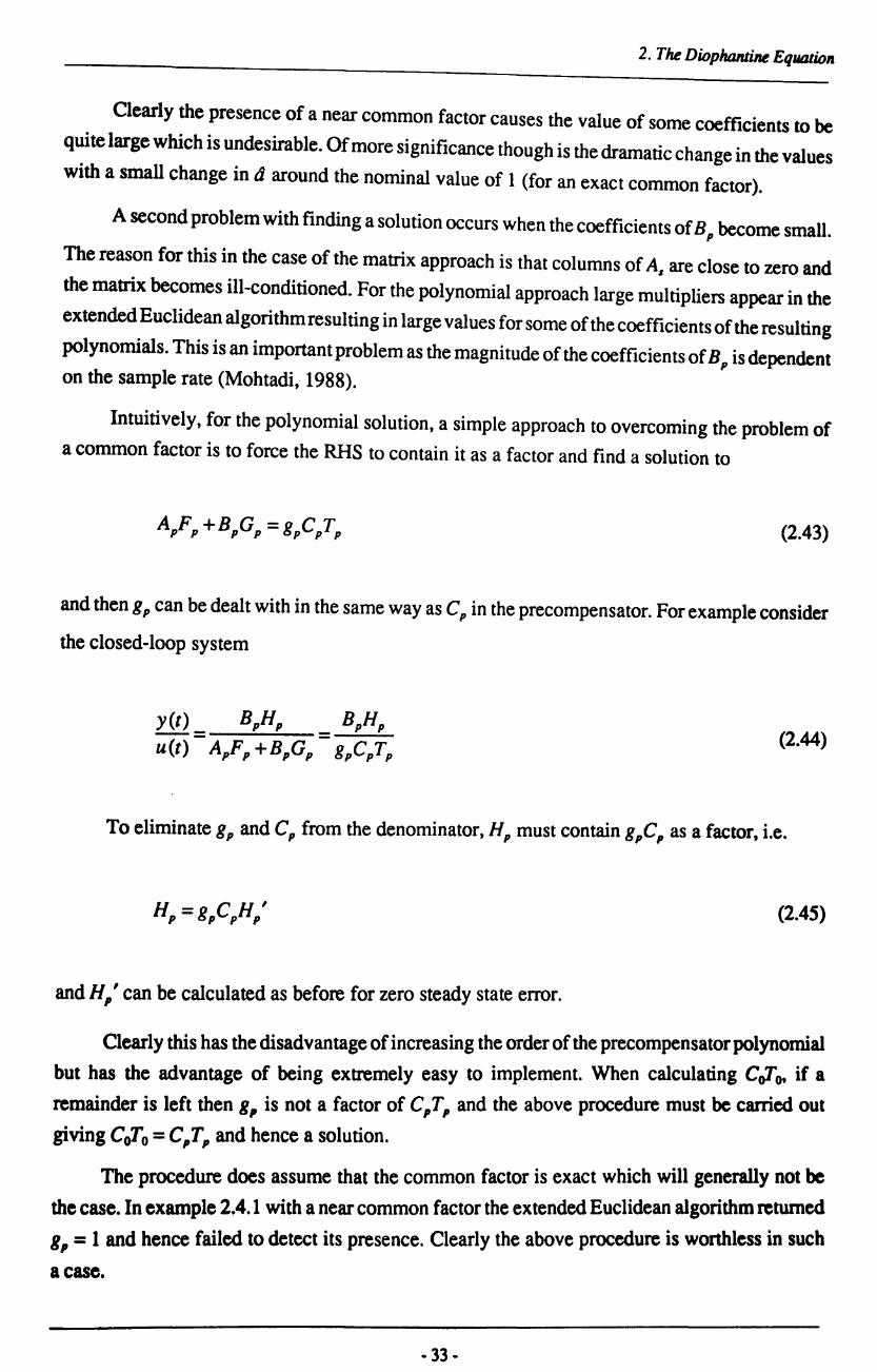
Clearly the presence of a near common factor causes the value of some coefficients to be
quite large which is undesirable. Of more significance though is the dramatic change in the values
with a small change in d around the nominal value of 1 (for an exact common factor).
A second problem with finding a solution occurs when the coefficients of B p become small.
The reason for this in the case of the matrix approach is that columns of As are close to zero and
the matrix becomes ill-conditioned. For the polynomial approach large multipliers appear in the
extended Euclidean algorithm resulting in large values for some of the coefficients of the resulting
polynomials. This is an important problem as the magnitude of the coefficients of B p is dependent on the sample rate (Mohtadi, 1988).
Intuitively, for the polynomial solution, a simple approach to overcoming the problem of
a common factor is to force the RHS to contain it as a factor and find a solution to
(2.43)
and then g p can be dealt with in the same way as C p in the precompensator. For example consider
the closed-loop system
(2.44)
To eliminate gp and Cp from the denominator, Hp must contain gpCp as a factor, i.e.
and H ' can be calculated as before for zero steady state error. ,
(2.45)
Clearly this has the disadvantage of increasing the order of the precompensator polynomial
but has the advantage of being extremely easy to implement. When calculating Cr:to, if a
remainder is left then g, is not a factor of C,Tp and the above procedure must be carried out
giving CoTo = CpTp and hence a solution.
The procedure does assume that the common factor is exact which will generally not be
the case. In example 2.4.1 with a near common factor the extended Euclidean algorithm returned
H, = 1 and hence failed to detect its presence. Clearly the above procedure is worthless in such
I case.
·33·

2. The DiophantiM EqUlJlion
For the matrix approach the only complete solution is to isolate the offending common
factor in Ap and B p and remove it from the polynomials before constructing the simultaneous
equations (Tuffs, 1984). Again this relies on having an exact common factor so is not appropriate for practical problems.
It is possible to fonnulate a recursive solution to (2.1) by introducing an arbitrary signal
;(t) to produce a regression model (Edmunds, 1976; Alix et ai, 1982)
(2.46)
where et(t) = C pTp~(t), a (t) = Ap~(t) and b (t) = B p~(t).
This can then be used as the basis of a recursive estimator with a parameter vector [F p G p],
a measurement et (t) and a data vector
[aCt) a(t-l) ... b(t-td) b(t-td-l) ... ] (2.47)
The problem of a common factor is also present in this framework and appears as linear
dependence in the data vector. Theorem 2.1 showed that no solution exists unless the common
factor is also a factor of the RHS so it is reasonable to expect the estimator to experience some
difficulty in converging to a solution as in fact none exists.
Another approach (Lawson and Hanson, 1974; Tuffs, 1984) is to examine the 'pseudo
rank' l of the A" matrix and if a rank deficiency is detected, calculate a 'minimum-nonn' solution,
i which minimises the Euclidean length of Ii = b - A"i. Such a solution is numerically very
robust. The major drawback here is that it has not been proved that the closed-loop system is
stable under all conditions.
Berger (1988) suggests splitting the desired closed-loop poles into two parts J, and K,.
The fIrSt part, J, is chosen to satisfy the desired design criteria whilst K" the second part, is
initially set to zero but can be adjusted to improve the conditioning of the set of linear equations.
It is necessary to specify bounds for the coefficients of K r
For the problem of small B, coefficients due to rapid sampling (which can also give rise
to a common factor), Middleton and Goodwin (1986) have proposed a method which involves
replacing the Z-1 operator with the a operator which is defined as
1 Lawson and Hanson (1974) define the pseudo-rank of a matrix A to be the rank of a matrix A that replaces A as a result of a specific computational algorithm.
- 34-
z-1 0=e
2. The Diophantine Equation
(2.48)
where e is the sampling interval. It is claimed that the use of this operator gives rise to a number
of benefits including improved finite word length characteristics and an improvement in the
conditioning of the sylvester matrix. Of course the implementation of control strategies in the 0 operator are more complex than those in the more common shift operator.
There are many other discussions of the diophantine equation and its properties in the
literature together with a number of proposed methods for overcoming the problems associated
with finding a solution. Such a proliferation of methods indicates that no one approach can deal
with all the shortcomings of this equation and that the calculation of its solution should be carried
out with some care.
2.5 Obtaining a More Robust Solution
Putting aside the problems associated with the equation, another interesting aspect is the
number of possible solutions as highlighted by theorem 2.2. As a first step towards the goal of
designing polynomial controllers with improved performance robustness, it would be interesting
to investigate the robustness properties of various solutions to the diophantine equation.
The matrix approach appears to be the more popular method of solving the equation. This
is probably due to a greater general familiarity with the theory of matrices, the fact that the matrix
representation of the equation is of a standard form and lastly because the matrix method is more
easily implemented on a computer. Thus it seems appropriate to base the investigation on this
approach. It is assumed that there are no problems with common factors or small coefficients
and so standard matrix analysis is used to solve the equation.
Based on this method for solving the equation, the effect of errors (or perturbations) in the
model parameters is considered which helps to establish a suitable robustness criteria. It will be
seen that vector and matrix norms play an important role in the evaluation of this criteria and so
a brief discussion and definition of them is included, followed by some comments on how to
select alternative solutions. A set of results using the proposed robustness criteria are presented
for a number of examples and conclusions drawn about the suitability of such an approach for
improving performance robustness.
- 35 -

2. The Diopharuine Equation
2.S.1 The Effect of Parameter Perturbations
If the parameters are subject to perturbations then the matrix equation (2.31) can be
represented as
(2.49)
where As, x and b represent the true values and Ms, & and M the errors.
Itis necessary to establish some sort of measure to gauge the robustness of various solutions.
The matrix form of the diophantine equation is of a standard form on which much work has been
carried out. Perturbation theory for linear systems can be used to help establish the appropriate
criteria.
A suitable measure of robustness could be obtained by computing an upper bound for the
relative perturbation II & II III x II. There are a number of such bounds, the following is taken from
a derivation in Lancaster and Tismenetsky (1985).
Subtracting As:! = b from (2.49) gives
(As + Ms)ilx +M~x = M (2.50)
or
(2.51)
Lancaster and Tismenetsky (1985) show that the existence of (I + As-1 Msfl is implied if
(2.52)
where the particular norm used must satisfy
11/11 = 1 (2.53)
Also
II (I + As-IMsfl II < (1- prl (2.54)
- 36 -

Thus
& = (/ + A -1M )-IA -1M - (/ + A -1M )-IA -I A A - I I I _ Iss L.lt'1s:!
and if 11·11" is any vector norm compatible with 11.11,
As:! = b implies that II b II " < II As II II x II" hence
Thus
1I£1!.1I" < II AsIIIIA;111 .II~II" +_P_ IIxll" - I-p IIbll" I-p
2. The Diophantine EqUlJlion
(2.55)
(2.56)
(2.57)
(2.58)
Define K(A.r) = II As II II A;ll1 to be the condition number of A.r and note that
p = II A;'IIII M,U = 1C(Ai~,~,11 (2.59)
Thus
(2.60)
It would seem reasonable to suggest that the solution which minimises the upper boun~
U. is the most robust solution as this minimises the maximum possible variation in x.
·37 -

2. The Diopharuine Equation
However, these results are really only valid for small perturbations in As and b. As the
relative perturbation of A, increases, there will come a point when the evaluation of Ub will return
a negative value, due to K(As) II Msil /11 Asil becoming> 1. The relative perturbation of x should
always be positive, thus the value of Ub will be invalid.
At this point it is worth noting that the essential difference between sensitivity and
robustness analysis is that sensitivity based results are concerned with small perturbations,
whereas more significant parameter variations are considered with robust design techniques.
The above perturbation theory gives rise to a sensitivity result, hence the upper bound becoming
invalid for larger changes. However, sensitivity analysis can provide a useful insight into
appropriate robustness measures.
Upon closer examination of the expression for Vb it can be seen that the condition number
of As has a large influence on the upper bound of the relative perturbation of x. Based on this
observation and the knowledge of the benefits of achieving well conditioned matrices, it would
seem reasonable to suggest that the conditioning of the sylvester matrix would be a useful measure
of robustness for systems with not necessarily small parameter perturbations.
2.5.2 Matrix and Vector Nornls
The upper bound, Ub of the relative perturbation and the condition number depend on
vector and matrix norms, of which there are many. The most commonly used matrix norms are
P or Holder norms and the Frobenius or Euclidean norm.
The P norm is defined as
IIA!.II p
IIAllp = !~~ Ilxll p
for any x, where II xii p = (I XII p + ... + I xnl p)lIP and p is generally taken as p = 1,2 or 00.
The Frobenius norm is defined as
- 3X -
(2.61)
(2.62)

2. The Diophantine Eqlllltioll
However because of the assumption in (2.53) that II/II = 1 the Frobenius norm cannot be
used as II/II F = n 112. Essentially the aim here is to find the minimum condition number and it is
well known (Golub and Van Loan, 1983; Horn and Johnson, 1985) that if a point is a minimum
with respect to one norm it will also be a minimum with respect to another norm. This equivalence
of norms means that anyone of the p norms could be used to calculate the condition number and
select the most robust solution.
2.S.3 Selecting the Order of the Controller Polynomials
A common approach to solving equation (2.31) is to use the minimum order solution
(Kucera, 1979; Wellstead and Sanoff, 1981; Clarke, 1982) where
(2.63)
(2.64)
although a number of other authors have proposed using alternative solutions (for example
Astrom and Wittenmark, 1980; McDermott and Mellichamp, 1984; Warwick et ai, 1985). The
choice of which solution is 'best' is still an area of on-going research and of course will depend
on the design objectives.
To select other solutions the orders of F p and G p will have to be changed. For the matrix
equation this will mean changing the dimension of the matrix and vectors. Thus it is necessary
to understand the conditions under which n/ and n, can be selected.
In equation (2.31), the number of columns containing Ap coefficients = the number of F,
coefficients = n/ + 1, and the number of columns containing B p coefficients = the number of G,
coefficients = n, + 1.
i.e. (2.65)
where Nt: = the number of columns and N" = the number of unknowns.
The number of A, coefficients = n. + 1, and B, coefficients = n" + 1. Again examining
equation (2.31) it is clear that the coefficients are moved down by one row for each successive
column, therefore the number of extra rows created is n/ for the A, coefficients and n, for the
B, coefficients.
- 39-

2. The Diophantine EqlllJlion
. I.e. (2.66)
where N, = the number of rows and Ne = the number of equations.
From equation (2.29) it is clear that the two values in the brackets will be equal, so either can be used.
As the number of rows and columns are affected there are three possible situations that could arise, assuming that A" is of full rank:
i) The number of rows = the number of columns
and n =n -1 g a
and a solution can be easily obtained. This case only occurs for the minimum order
solution.
ii) The number of rows < the number of columns
This corresponds to the case where the number of unknowns > the number of
equations, thus by setting some of the unknowns arbitrarily it is possible to easily
obtain a solution.
iii) The number of rows> the number of columns
In this case there are more equations than unknowns, which can lead to problems
of inconsistency where a set of values for the unknowns is obtained which do not
satisfy all of the equations. To guarantee that such problems do not arise it is
necessary to investigate the conditions under which this case will never occur.
Limits for n, and ng such that the number of rows ~ the number of columns are
and n, ~ n.-l
As n, = n. - 1 and n, = nil - I are the minimum order solution, these conditions will
always be fulfilled and case iii) can never occur.
Suitable choices for n, and n, can be deduced from the conditions mentioned above. To
summarise, all of the following constraints must be satisfied :
-40-

2. The Diophanline Equalion
a) n" + nj = nb + ng
b) ng ~ n,,-l
c) nj ~ nb-1
d) if Nu > N. then some of the unknowns must be arbitrarily assigned
The fIrSt constraint means that if the order of F p is increased then the order of G p must be
increased by the same amount.
2.5.4 Simulation Results
Three examples are considered
1) A non-minimum phase system (taken from Wellstead and Sanoff, 1981)
(1-1.6z-1 + 0.6z-2)y(t) = (Z-1 + 1.5z-2)u(t) + (1 - OAz-1)e(t)
and it is desired to have a closed loop pole at 0.8
(2.67)
It is assumed that the Ap, Bp and Cp polynomial coefficients are subject to uniformly
distributed random perturbations of 2%,5% and then 15%.
2) A system proposed by Berger (1984)
(1-2z-1 +Z-2)y(t) = (Z-1 +0.1z-2)u(t)
and the desired closed loop poles are all assumed to be zero.
(2.68)
The Ap ' B p polynomial coefficients are now assumed to be subject to normally dis
tributed random perturbations with variances of firstly 0.01 % and 0.02% respectively
and then 5% and 10% respectively.
3) A hydraulic rig (taken from Daley, 1987)
(1-0.54666z-1)y(t) = (1.28621z-1)u(t)
and the desired closed loop pole positions are 0.75 + jO.2
(2.69)
The Ap ' B, polynomial coefficients are time-varying with respect to the supply
pressure. The relative size of the variations are 10% and 125% respectively.
-41-

2. The Diophantine Equation
A digital integrator is cascaded with each system to achieve the desired steady state
perfonnance as outlined in section 1.2, hence two closed loop poles being specified for example
3 which is a fIrst order system.
The minimum order solution is unique, however when nl and ng are increased beyond their
minimum order values, a set of solutions is obtained. The size of the set increases as nl and n,
increase. Consider the case where nl and ng are increased by one from their minimum order
values. This particular set of solutions will be referred to as the minimum order + 1 solutions.
Section 2.5.3 outlined how the size of equation (2.31) was affected by changes in nl and n,. From
this work, in particular equations (2.65) and (2.66), it is clear that the number of unknowns in
equation (2.31) increases by two whereas the number of individual equations (or rows of the
matrix A.) only increases by one. In order to solve equation (2.31) for a particular solution it is
necessary to arbitrarily set one of the unknowns. The mathematics involved can be greatly
simplified if the unknown is set to zero as this is equivalent to deleting one of the columns from
the sylvester matrix As. It is important to ensure that the resulting square sylvester matrix is of
full rank, else the solution will suffer from numerical problems as outlined in section 2.4.
If nl and ng are increased by two from their minimum order values then the minimum order
+ 2 set of solutions is obtained. In this case it is necessary to arbitrarily set two of the unknowns,
and if zero is again used this translates to deleting two columns from the sylvester matrix.
It is possible to continue increasing nl and ng resulting in even larger sets of solutions.
However, for the purposes of this investigation only solutions up to and including the minimum
order + 2 set will be used, as this should give a sufficient indication of the performance of the
robustness measures and the suitability of this approach.
The levels of perturbation specified for examples 1 and 3 define the approximate level of
random perturbation required, and for example 2 the actual variance of the perturbation is given.
On the basis of this, four sets of random perturbations are generated for each example to allow
a better investigation into the correlation between the measures of robustness (condition number
and upper bound) and the true relative perturbation. This results in four plots appearing in each
figure corresponding to the four sets of random perturbations.
For the minimum order + 1 solutions the x -axis on the graphs corresponds to which column
was deleted from the sylvester matrix. However, as to is fixed at 1, column 1 was not actually
deleted and in its place are the results for the minimum order solution. For the minimum order
+ 2 solutions the x-axis can no longer be used to indicate which columns are deleted as it is now
necessary to remove two. Instead all possible solutions are shown in no particular order except
that the minimum order solution is still first. The 2-norm was used for calculating the condition
number and upper bound throughout. The graphs are located at the end of the chapter.
-42 -

2. The DiophanJine Equalion
The 2% perturbation results for example 1 are shown in figures 2.1 and 2.2. The upper
bound and the condition number agree quite well with the lowest minima indicating the best
solutions. From the graph of the true relative perturbation it appears that the measures are
generally selecting good solutions as regards robustness. Figures 2.3 and 2.4 show the 5%
perturbation results. The upper bound is only valid for the minimum order + 1 solutions where
there is good agreement with the condition number on which solutions are better. The upper
bound for the minimum order + 2 solutions demonstrates the effect of higher levels of pertur
bation, highlighting its inadequacy as a robustness measure. Comparing the condition number
and the true relative perturbation, it can again be seen that generally the condition number selects
the better solutions. When the level of perturbation is increased still further to 15% (figures 2.5
and 2.6) the upper bound becomes totally invalid for all solutions. Again the results show a good
correlation between the condition number and the true relative perturbation.
Moving on to the second example, the results for a low level of perturbation are shown in
figures 2.7 and 2.8. Even at this level of perturbation the upper bound is not valid for all solutions
and so should be ignored. Comparing the condition number and the true relative perturbation it
can be seen that the correlation between the two is not as good as for the first example. Figures
2.9 and 2.10 show the results with a higher level of perturbation and again the same conclusions
can be drawn when comparing the condition number and the true relative perturbation.
Lastly in figures 2.11 and 2.14 the results for the third example are given. As would be
expected, due to the high level of perturbation for this example, the upper bound is again invalid.
There is a slightly better correlation between the condition number and the true relative per
turbation than for example 2, but still not as good as for example 1.
2.6 Conclusions
Having established that the diophantine equation is important in the calculation of a
pole-placement controller, this chapter has outlined some important points regarding the equation
and obtaining a solution to it. Such an understanding is useful when considering the problem of
robustness.
There are two approaches to solving the equation, polynomial methods and matrix methods.
Neither appears to have any distinct advantages although the matrix approach seems to be more
popular, possibly due to the greater general familiarity with matrix theory, the fact that the matrix
representation of the equation is of a standard form and also because the matrix approach is
easier to implement on a computer.
- 43 -

2. The Diophantine EqUlllion
A solution to the equation only exists if Ap and Bp are coprime or if the right hand side
contains their common factor. The consequence of this statement only becomes apparent when
it is understood how common factors can arise for discrete time systems. It is clear that the sample
time plays an important role in the occurrence of such factors and so should be chosen carefully.
With exact common factors it is possible to easily detect and overcome their presence,
however it is more likely that near common factors will be present which show themselves as
ill-conditioning of the matrix equation. Many techniques have been proposed for the case of near
common factors but no one method appears to have totally overcome the range of possible
problems that could be encountered.
The occurrence of small Bp polynomial coefficients also causes problems when trying to
solve the equation, which is important as the magnitude of the Bp coefficients is also a function
of sample time. Obtaining a solution clearly suffers from a number of problems but putting them
aside, another interesting aspect is the number of possible solutions to the equation.
Any solution will meet the design objective by placing the poles in their desired locations,
but different solutions may have interesting properties from the point of view of additional design
goals. The goal in this case is to find controllers where the closed-loop transient response is
robust to changes in the open-loop model parameters.
From the derivation of an upper bound on the relative perturbation of the solution to the
matrix form of the equation, it can be seen that the conditioning of the sylvester matrix is
important. An investigation into obtaining better conditioned matrices by changing the order of
F p and G p is then presented. Although the correlation between the conditioning and the true
relative perturbation was not perfect, it is clear that the commonly used minimum order solution
is not necessarily the best in this sense.
However this is really only addressing the problem of numerical robustness in the sense
that the controller polynomial coefficients will be less affected by changes in the model poly
nomial coefficients. This is certainly a desirable property to achieve but its effect on the stated
goal is difficult to assess. The transient response is dependent on a number of factors, one of
which is the poles of the system, i.e. the roots of the characteristic polynomial. Minimising the
change in the characteristic polynomial's coefficients does not necessarily minimise the change
in the roots (or pole positions). The reason for this is that the relationship between the roots of
a polynomial and its coefficients is not a simple one.
It is clear that an alternative approach is needed which can investigate the effect of model
parameter perturbations on the factors that directly effect the transient response. There is a
growing interest in parameter space methods (Siljak, 1989) which, in the algebraic framework,
-44 -

2. The Diophantine Equalion
relates the changes in the coefficients of a polynomial to changes in the roots. However the
transient response is not solely dependent on the pole positions so this approach would not enable
a full investigation into transient response robustness.
-45 -

2. The DiophanJi~ EqUtJlion
Condition Number
35r-------~--------~--------~------~--------~------~
:' ".
101t------------2~----------~3~----------~4~----------~S~----------~6~--------~7
Upper Bound of the Relative Perturbation
0.4r---------~----------~--------~----------~--------~--------~
0.051~----------~2------------~3~----------~4~----------~S~----------~6~----------J7
True Relative Perturbation
0.055r-----------~------------~----------~~----------~----------~~----------~
0.05
0.045
0.04
0.015
0.01
..... ".
.. ' ",
...... . ,.,
.. --.'
'" "
0.OO51L------------~2----------~3~----------~4~----------~------------6~----------~7
Figure 2.1 - Min Order + 1 Solutions for Example 1 (2% Perturbation)
-46-

2. The Diophantine EqlllJlion
Condition Number
90r---~----~----~--~----~----~--~----~----~--~
Upper Bound of the Relative Perturbation
3.5
3
2.5
2
loS
1
0.5
00 2 4 6 20
True Relative Perturbation
0.09r-----~-------r------~----~------~------~----~------~------~----~
0.08
0.07 0.06
0.05
0.04
0.03
0.02
.... . ................... .. ......... . .....•
......... ..... " ............ . . ... . .... ...... ..... ............ .
" .... ....
0.01
16 18 2 4 6 8 10 12 14
Figure 2.2 - Min Order + 2 Solutions for Example 1 (2% Perturbation)
·47·

2. The Diop~ Equation
Condition Number
3Sr-------~--------~--------~------~--______ ~----__ ~
30
. " " ....
101t------------:2~----------~3~-----------4~----------~S~----------~6~----------J7
Upper Bound of the Relative Perturbation
14r---------~----------~--------_r----------~--------~--------~ .' .
12
10
8
6
4 .....
..•..
..... ....
. -2 ."" ..... -
.. '
" . ".
.'" .... i .
" .... ... " i' i'
" " .. ~'" /"
i i
.. ' " ."
.. / '.
" "
"":>', ,,' ":'\I!. .. '.~ .... , ....... ~. _ ... _. __ .......
°1~=-~-~-~-~-~-~-~-~-~-~-~;~-~-~-~-~-~-~-~-~-~-~-:-~3~~~~~~~4~~~~~~~s~~~~~~~6~~~~::~d7 .;;:(~/ ------
True Relative Perturbation
0.14r-----------~------------~----------~------------~----------~~----------~
0.12
0.1
0.08
0.06
0.04 ... '
0.02
'. ............................................
.......... . ..... ,. ...... ~.-'" ....... .' .
. ..... .
-' -
....
..-.. '
.. '
.... . ..•..
......
' .
".
------------------------------------------------- --. 2 3 4
......... - _ .. -'.'''''-'.' ..... - _ .... - .... -
.............. ,.,' ,., ......... -, .. .
------------------------6 7
Figure 2.3 - Min Order + 1 Solutions for Example 1 (5% Perturbation)
·48 -

2. The Diophantine EqUlllion
Condition Number 90
80
70
60
50
40
30
20
100 10 12 14 16 18 20
Upper Bound of the Relative Perturbation
20r-----~------~----~------~----~------~----~------~----~----~
-20
-40
-60
-"
~~:::\'~T· • l \1. .' !
! f \ ; , .i
_ •••• # •
r· ... • _____ = o
, ; -80 \I ,
,*! - - - - = .' .. ,. \ ...••. \. '-. ... //
~ ',..-..... : i i
\ / ;
\ : v
........ --',..
-1000~------~2~----~4~----~6~------8~----~1~0~----~1~2~----~1~4------71~6~----~1~8~----~20
True Relative Perturbation
0.16r-------,-------~------_r------_T------~------~~------~------r_------T_----~
0.08
0.06
0.04
... i' ...
l \, ,i '
", '~'''' .' .. _ .. _ ...... _ .. _ --._ ......... 1
! \ , / .. ' ' ..... ':;, ... ~:~-~:.:~:.;~: .. : .. ' \ ...
-.,.-;--....... .... ......... "" ........... .::... ................. ... - - - - - - - - - - ... - - - - __ - ... .. ............ ",,# - - - - - - -
...... -- ----- .,' .•.......... . ..... . ...........
4 6 8 10 12 14 16 18
Figure 2.4 - Min Order + 2 Solutions for Example 1 (5% Penurbation)
·49·
20
2. The DiophanJine EqUiJlion
Condition Number
40~--------~--------~--------~------__ ~ ________ ~ ______ ~
35
30
2.5
2.0
Upper Bound of the Relative Perturbation
.. " . ..•. . ,. .....
.. - .0-
7
2.0r-----------~--------~~--------~----------~----------~-----------
----- _________________ ~---~-r------'. \ \
-40 .•.
-60
-so
-100
-12.0
-140
-160
-lS01~-----------2~----------~3~----------~4~----------~S~----------~6~----------~7
True Relative Perturbation
0.22.r-----------~------------~----------~~----------~------------~----------~
0.2.
O.lS
o.os
0.06
0.04
3 4
.- -.- -----'-. , ... - -'-
-----------------
6 7
Figure 2.5 - Min Order + 1 Solutions for Example 1 (15% Perturbation)
·50·

100
90
80
70
60
50
40
30
20
10 0 2 4
20
10
0
-10
-20
-30
-400 2 4
2. The Diophanline EqUillion
Condition Number
20
Upper Bound of the Relative Perturbation
-' . -.' ·oJ .',' :", \\
\ ... . ------------':'~ ... ' ,-,"~----..... \ \ \ \
\ \
6 8 10 12 14 16 18 20
True Relative Perturbation
0.35r-----~------~------_r------~------~----~------~------~------T_----~
0.3
0.25
0.2
0.15
0.1
..... '. ..... . .... .. : .....
· · · · ·
" . .. '
.....
" . .......... .
/ ! \ '-.~~o~_~.:-~.-~.-~.:-~.~ __ ~~.~ .. ~ .. :.~.~.-~~~----~ "/' ' .. . _._ ... o.-._ .. ·i·····-··~·':;··· .... ............. .".-, i \ , _. ...........t "''' ... I - ____ , ........ .. _-- ----_ .............. ---- ... -- "'-"
,- --- - - - --
, \
. ..... ....
• o'
". ""--_ .. _----0.050~------~2------~4~------6~------~8-------1~0------~1~2-------1~4-------1~6-------1·8------~20
Figure 2.6 - Min Order + 2 Solutions for Example 1 (15% Perturbation)
- 51 -

400
350
300
250
200
150
100
50
0 1 2
40
30 I-
20 I-
10~
0
-lOt-
-20 1 2
Condition Number
3 4 S
Upper Bound of the Relative Perturbation
...
:
3
.. .. ~ .... ..
4
.• ..
True Relative Perturbation
2. The Diophantine EqUIJtion
6
6
7
-
".:.-- - - - - ----~ '" '- . ...... .... ,
7
0.045r---------------------~----------~--------~----------~----------
0.04
0.035
0.02
0.01 ................ " ....... " . • ••••••• 0'
.' .'
.....
, '
.'.
".
. ..... .
, -' - ... - .. ","",. _.- ...... -.... -',
. ...... ....... . ............. , -... . ........... . ------- ----------------------------...,.- ------
-------------------------------- ----. 0.0051~--------~2~--------~3~--------~4----------~5~---------6~--------~7
Figure 2.7 - Min Order + 1 Solutions for Example 2 (0.01 % & 0.02% Perturbation)
·52·

2. The DioplratatiM Eqlllllion
Condition Number
500
450
400
350
300
250
200
150
100
50
00 2 4 6 8 10 12 20
Upper Bound of the Relative Perturbation
60r-----~----~-r;--~~----~----~----~------~----~----~----~
i 50 ;
40
30
True Relative Perturbation
0.05r-----~------~------~----~------~------~----~--~--~----~~----~ ......... ' ..
0.045
0.04
0.035
0,03
0.025 0.02
0.015
0.01
. " .........
\, \\. \ ........................ .
...... " . '". . ......... .
.... ",,' ......... ....... .' -........ _---
' . ..... . _._ ...
",.- .. '. . '.
' .. ''''"
\,
....... , ....... . ....
\,
.. ..........
" ...... '" ~,------- ..... - .............. . .. -- - --... .,' ,," ............ - --------
"",,'" ........... '. -,,' "" ..... _--------"," ............
0.0050~----~2-------4~-----6~----~8-------1~0------1~2------1~4------~16-------1~.----~20
Figure 2.8 - Min Order + 2 Solutions for Example 2 (0.01 % & 0.02% Perturbation)
• S3·

2. The Diophantine Equation
Condition Number
500r-------~--:_----~-----,--~------~--------~--------
450
400
350
300
250
200
150
100
50 r--...... _..;...;.;.;::.;.;.:;.:.:t
I i i
- - - - - - -.- - - -
.. ' ........
.................. °1~-----------2~----------~3~----------~4~----------~S~---··-··-··-··-··-··-·-·~6~--------~7
Upper Bound of the Relative Perturbation
-1r-------~------~~------~------~--------~------~
-1.05
-1.1 ..... ....
-1.15
-1.2
-1.3
-1.35
.....
"........ ", ...... . ............................... .
. .... .. '
..' .. ,
-1.41~----------~2------------~3~----------~4~----------~S~----------~6~----------~7
True Relative Perturbation
1.4r-----------,-----------~----------~----------~-----------r----------~
1.2~
..... 1~
.... ..... .......
0.8~
0.6~
~ .•. -... - .. ' .' 0.4 ~- '-"' .....•.•...•
0.2~
----
....
-----------.. -
-..' ..... . ....... .
" ....... .
-
-.•.•..... _ .. - . -
----------------------------- -----
------------------------------°1~----------~2------------~3~----------~4~-----------5~-----------6~----------~7
Figure 2.9 - Min Order + 1 Solutions for Example 2 (5% & 10% Penurbation)
·54-

2. The Diophantine Eqlllllio"
Condition Number
1400r-----~----~----~----~--~~~----~--~~----~----~----~
1200
1000
800
600
400
200
\ \
~
, ,
Upper Bound of the Relative Perturbation
-1.60~----~2~----~4------~6~----~8~----~1~O~----~1~2----~1~4------~1~6-----1~8------2~0
True Relative Perturbation
1.4r-----~~----~-------r------~------~----~~----~------~------~----~
0.6
0.4
0.2
..........
.... ". .................
. .............. . . ... . ...
. ....
.,<" - - -'-. _. - - _._._ .... - ..... ....... --~......:.:.~-...:.:.:-"-'-"--~../ ........ __ ..--
,.,r - - - - ............ ~ ....... -",............... ", ...... _--_............. ..------ "" ... _------ ...
,. ---------,,' .... _-----_... "'-- .. ' 2 4 6 8 10 12 14 16 18
Figure 2.10 - Min Order + 2 Solutions for Example 2 (5% & 10% Penurbation)
·55 -

2. The DiophantiM EqllQlion
Condition Number
3~r-----~~----~------~------~------~----__ ~ ______ ~ ____ ~ 30
2~
20
1~
10
~ ............ .
.. ' -----------...... -----------
.'
"
........
°1L-------l1~.S~------~2------~2~.cS------~3~----~3~.~S~----~4~------~~----~
Upper Bound of the Relative Perturbation
3r-------~------~------~--------~------~------~------~------~ 2
1
-------------------------- -------o
-1
-2
-3
-4
-~
-6
-71~------71~.S~------=2------~2~.S~------~3~----~3~.~S~----~4~------4~.~s~----~
True Relative Perturbation
0.25r-------~--------~------~--------~------~~------~--------~------~
0.2 - . ' . ... ............. - - ..... - .... ,.
0.15 -
0.1 ~
0.05 ~ ... . .....
...
".
. ....
- .,.'-
. ,.' .. ' . .....
-. .•... -- .... -
-
-..... :.:.
--------------------------------------------------1.5 2 2.S 3 3 • .5 4 4.5 5
Figure 2.11 - Min Order + 1 Solutions for Example 3
- S6-

2, The Diophantine Equation
Condition Number
4Or-----~------~------~------~------~--__ ~------~ 35
30
25 ........ .. ' ... ' .' ....
20 ~.' ... .'
-'-15 -. -....
10
5 "-'::"::"::"::"::':'"
,.' " ..
"'''''
------:..':..------
", .
... ------
'.
. ....
°1~----------------~2~------------~3~------------~4--------~S~--------6~------------~7~------~8
Upper Bound of the Relative Perturbation
5
-5
-10
-15
-201~----------------~2--------------------3~------------~4--------------S~-6 7 8
True Relative Perturbation
0.3r-----------~----------------_r----------------~--------------~~--------------~------------~----------~
''''" 0.25 - .•.•.
0.2 -
0.15 r
0.1 f-
' ..
..... .....
0.05 -
' . ....... ..... ,.
.....
..... .....
.. -'-'''''- -.- - - ~ ~ -.
.............................
-........ _ ..... - - .... -. .... -'''''
", ..... ..... . ...
... .............. . ......... -. '. " .
-
-
. .....
-
-r-------.. ..... --............. ----=-.:-:-:_:::~7~:_: __ :-:_~_~_:-_ -::-:-:-:-:-:------------------:.::..:.::.::.::.:..:..: :.::.::.::.::.::.: :.::.::.::.:-:" °1~--------~----------~3=---------------~4~----------~5~--------------~6~----------~7~--------~.
Figure 2.12 - Min Order + 2 Solutions for Example 3
• S7-

REFERENCES
Astrom, KJ., Hagander, P. and Stemby, J. (1984)
'Zeros of sampled systems' Automatica, v20, nl, pp 31-38
Astrom, KJ. and Wittenmark, B. (1980)
'Self-Tuning Controllers based on Pole-Zero Placement' lEE Proceedings, v127, Pt D, n3, pp 120-130
Astrom, KJ. and Wittenmark, B. (1989) , Adaptive Control'
Addison-Wesley, Wokingham, UK.
Alix, F., Dion, J.M., Dugard, L. and Landau, J.D. (1982)
2. The DiophanlilU! EqutUioll
'Adaptive Control of Non Minimum Phase Systems Comparison of Several Algorithms and Improvements '
Ricerche Di Automatica, v 13, n 1, pp 173-189
Berger, C.S. (1984) 'Robust Controller Design by Minimisation of the variation of the Coefficients of the Closed-Loop
Characteristic Equation' lEE Proceedings, v131, Pt D, n3, pp 103-106
Berger, C.S. (1988) 'Robust Pole-Placement Algorithm for Adaptive Control' lEE Proceedings, v135, Pt D, n6, pp 493-498
Clarke, D.W. (1982) 'Model Following and Pole-Placement Self-Tuners' Optimal Control Applications and Methods, v3, pp 323-335
Daley, S. (1987) , Application of a Fast Self-Tuning Control Algorithm to a Hydraulic Test Rig' Proceedings of the Institution of Mechanical Engineers, v201, n4, pp 285-295
Edmunds, J.M. (1976) 'Digital Adaptive Pole-Shifting Regulators'
PhD Thesis, Control Systems Centre, UMIST, U.K.
Golub. G.H. and Van Loan, C.F. (1983)
'Matrix Computations' North Oxford Academic Publishing, Oxford, U.K.
Hom, R.A. and Johnson, C.A.(1985)
'Matrix Analysis' Cambridge University Press, Cambridge, U.K.
Kucera, V. (1979) 'Discrete Linear Control: The Polynomial Equation Approach'
Wiley. Chichester. UX.
Lancaster, P. and Tismenetsky. M. (1985)
'The Theory of Matrices' Academic Press, London, U X.
·58 -

Lawson, C.L. and Hanson, RJ. (1974) 'Solving Least-Squares Problems'
Prentice-Hall, London, U.K.
McDermott, P.E. and Mellichamp, D.A. (1984)
'An Auto-Pole-Placement Self-Tuning Controller'
I nternational Journal of Control, v40, n6, pp 1131-1147
Middleton, R.H. and Goodwin, G.C. (1986)
2. The Diophantine EqUQIion
'Improved Finite Word Length Characteristics in Digital Control Using Delta Operators'
IEEE Transactions on Automatic Control, v31, nil, pp 1015-1021
Mohtadi, C. (1988) 'Numerical Algorithms in Self-Tuning Control'
Ch 4, 'Implementation of Self-Tuning Controllers' , Peregrinus, ed K. Warwick
NAG (1990) Fortran Library Manual Mk 14 Numerical Algorithms Group Ltd, Oxford, U.K.
Siljak, D.O. (1989) 'Parameter Space Methods for Robust Control Design: A Guided Tour'
IEEE Transactions on Automatic Control, v34, n7, pp 674-688
Tuffs, P.S (1984) 'Self-Tuning Control: Algorithms and Applications' PhD Thesis, Dept of Eng Science, University of Oxford, U.K.
Warwick, K., Farsi, M. and Karam, K.Z. (1985) , A Simplified Pole-Placement Self-Tuning Controller' lEE International Conference on Control' 85, Cambridge, U.K. vI pp 1-6
lEE, London, U.K. (Conf Publ No. 252)
Well stead, P.E. and Sanoff. S.P. (1981)
'Extended Self-Tuning Algorithm'
International Journal of Control, v34, n3, pp 433-455
- 59-

CHAPTER 3
STATE SPACE DESIGN FOR POLYNOMIAL SYSTEMS
3.1 Introduction
The previous chapter presented an initial investigation into obtaining controllers with
improved performance robustness by utilising alternative solutions to the diophantine equation.
The major conclusion was that although extra design freedom exists and it is easy to select
alternative controllers, the specification of a suitable robustness measure, on which to base the
choice of controller, was quite difficult. The main reason for this is that in the polynomial
framework there is no simple approach to assessing the effect of model uncertainty on the
response of the closed-loop system.
In a state space framework it is well known that the transient behaviour of a system is
governed by the eigenvalues and eigenvectors. Further, this description readily allows access to
these factors and hence provides a good basis for an investigation into improving performance
robustness. All of these points highlight the main reasons for turning to a state space based
approach for the design of robust polynomial controllers. Of course the polynomial description
of a system only provides a relationship between the input and output, so if state space methods
are to be used to design the controller polynomials it will be necessary to use an output feedback
approach.
The state space design needs to provide extra degrees of freedom which can then be utilised
as in the polynomial design outlined in the previous chapter to improve performance robustness.
There are a number of options and it is worth noting that any robust state space design method
could be used to illustrate the overall robust polynomial controller design procedure. Due to the
close link between the eigenstructure (eigenvalues and eigenvectors) and the transient response
it is natural to consider the techniques of eigenstructure assignment and parametric methods for
the state space design.
Of course it is necessary to define a suitable robustness measure on which to base the
selection of the extra design freedom. There are a number of possibilities for such a measure,
but as already mentioned the eigenvalues and eigenvectors are very important in detennining
the shape of the transient response and so it is reasonable to expect that they will play an important
role in the definition of a suitable measure. A complete discussion of this issue is presented in
the following chapter.
-60-

3. State Space Design for Polynomial Systems
In this chapter a more detailed explanation of the relationship between the eigenva
lues/eigenvectors and the transient response is given using modal decomposition, hence
emphasising the reasons for turning to a state space based design. A discussion of the overall
design with the transformation of the polynomial system to state space form and of the controller
back to polynomial form is then presented. An introduction to eigenstructure techniques is then
given, leading onto a discussion of parametric methods and in particular a review and comparison
of two specific parametric output feedback methods, followed by some conclusions on their
suitability.
3.2 Modal Decomposition
To understand the factors that effect the transient response, consider the modal decom
position of the discrete linear state space system (Kailath, 1980 and Ogata, 1987)
x(k + 1) = Ax(k) + B u(k)
y(k) = Cx(k)+Du(k)
Assuming the initial state is x (0) and the initial input is u(O), from equation (3.1)
x(1) =Ax(O)+Bu(O)
x(2) = Ax(1) + Bu(l)
= A 2X (0) + AB u (0) + B u (1)
x(3) =A~(2)+Bu(2)
=A 3x (0)+A 2Bu (0)+ABu(1) +Bu(2)
It is well known that
- 61 -
(3.1)
(3.2)
(3.3)
(3.4)
(3.5)
(3.6)
(3.7)

3. Siale Space Design for Polynomial Systems
where ~ are the eigenvalues and Y; the right eigenvectors of the matrix A, so clearly
AV=VA (3.8)
where V = [YI ... y,.] and A = diag[A.I ... A.n]. Therefore
(3.9)
Clearly A Ir. can be expressed by
(3.l0)
and substituting (3.9) gives
Air. = VAIr.V-1 (3.l1)
and as
WI
y-l = W = (3.12)
where !J are the left eigenrows of the matrix A ,
A.I 0 0 WI
A A: = £YI y.] 0 (3.13) .
0
0 0 A.II T ~
Thus
-62-

3. State Space Design/or Polynomial Systems
(3.14)
Clearly equation (3.6) becomes
(3.15)
and the output can be expressed as
(3.16)
Clearly the eigenvalues and eigenvectors are extremely important in detennining the shape
of the transient response. The eigenvalues affect the rate of decay and the eigenvectors the gain
associated with each mode.
Having shown the importance of the eigenvalues and eigenvectors, it is necessary to
establish the link between the two representations which will then allow a state space approach
to be used in the design of the controller polynomials.
3.3 The Link between Polynolnial and State Space Representations
The single-input single-output (SISO) polynomial system defined in equation (1.4) can be
expressed in observable canonical form, Ogata (1987), as
Xl 0 0 0 0 -a" Xl bIt -a"bo
x2 1 0 0 0 - a,,_l x2 b,,_l -all_lbo
- + u(k)
X,.-l 0 0 1 0 -~ X,,_l b2 -apo
x,. 0 0 0 1 -al x" l b1-a1bo
.+1
(3.17)
- 63-

3. State Space Design/or Polynomial Systems
y(k) = [0 0 o 1] (3.18)
where there are n states, m(= 1) inputs and r(= 1) outputs. Note that it is assumed that nG = nb = n
which can always be achieved by padding with zero terms if necessary. Also the time delay, td
will always be ~ 1 due to sampling and assuming the system is strictly proper, bo will always be
o as the time delay is included in Bp(Z-l). Hence in the analysis it is unnecessary to consider a
D matrix in the state space description.
It is well known that the poles of a closed-loop system may be arbitrarily placed by using
state feedback if and only if the system is controllable (Friedland, 1986). For output feedback
however it is also required that r + m > n, which can be achieved by adding a dynamic com
pensator of suitable order. Following Brasch and Pearson (1970), for convenience the com
pensator dynamics will be taken to be a number of integrators. It is also assumed that every state
in the compensator is observable and controllable. Therefore the new system with dynamic
compensator of order p can be represented as
(3.19)
(3.20)
where the dimension of x 1 is (n xl),:!2 is (p xl), U2 and Y2 are (p xl). Yl and U1 are scalars. 0; xj
indicates a zero block of dimension i x j and Ip indicates a p x p identity block.
Output feedback can then be applied via the control law
(3.21)
In state space fonn, the problem is then to determine the controller gain matrix K, which
places the closed-loop eigenvalues in the desired locations, and yields a closed-loop system
where the transient response is robust to changes in the elements of the A and B matrices.
·64·

3. State Space Design for Polynomial Systems
Once K., has been obtained via a suitable state space design method it is necessary to
interpret it in a polynomial framework. Note that the original input and output are U1 and Yl and
that the relationship between Y:2 and 0 is
~(k) = !h(k -1)
The control law can also be partitioned in a similar way
where the sub blocks of Ky are of appropriate dimension. Rewriting gives
u1(k) = K 11Yl(k) + K1ib,(k)
!h(k) =K21Yl(k)+K2ib,(k)
From (3.22) and (3.25) .
Hence (3.24) becomes
Which gives
·65 -
(3.22)
(3.23)
(3.24)
(3.25)
(3.26)
(3.27)
(3.28)

3. Slale Space Design/or Polynomial Systems
Thus giving the expressions for F/z-1) and G /Z-1). The precompensator polynomial,
Hp(Z-I) is calculated as before for zero steady state error.
3.4 State Space Design
Having shown in the previous sections how closely related the eigenvalues and eigenvectors
are to the transient response, and how state space methods can be used in the design of polynomial
controllers, the next step is to consider the actual state space design to be used.
The eigenvalues and eigenvectors are clearly very important as regards the transient
response, hence it is desirable to consider the placement of not only the eigenvalues but the
eigenvectors as well. Such a design procedure is more commonly known as eigenstructure
assignment (Burrows, 1990).
Consider the linear time invariant state space representation of a system
i =Ax+Bu (3.29)
(3.30)
where there are n states, m inputs, r ou tpu ts and A, B, C are matrices of appropriate dimensions.
The D matrix will be zero due to the nature of the transformation from polynomial to state space
form and the time delay of the system, as outlined in section 3.3. Output feedback can be applied
to the system via the control law
u=Ky - -(3.31)
Eigenstructure assignment can then be described as the assignment of the closed-loop
eigenvalues and eigenvectors (either left or right) using the control law (3.31).
Srinathkumar (1978) discusses eigenstructure assignment using output feedback and
concludes that min(n,m +r -1) eigenvalues may be arbitraily placed as well as (r -1) eigen
vectors partially assigned with m entries in each vector arbitraily chosen. Clearly for all n
eigenvalues to be arbitraily assigned using output feedback, r + m > n. This result was originally
obtained by Kimura (1975).
-66-

3. Slale Space Design/or Polynomial Sys~ms
Whilst the choice of a closed-loop eigenvalue may be arbitrary, under certain assumptions,
the corresponding closed-loop eigenvector is constrained to lie in a subspace of the full state
space. This subspace is tenned the allowable eigenvector subspace and Burrows (1990) discusses
in detail various approaches to detennining it and the corresponding controller gain matrix.
Of course having a technique for assigning the whole eigenstructure does open up the
question of what is the most suitable position for the eigenvalues and eigenvectors? The concept
of placing the eigenvalues (or poles) of a system is extremely well known and the effect on the
characteristics of a system for various eigenvalue locations is clearly understood. By selecting
appropriate eigenvectors it is hoped to achieve a system with better robustness properties.
However, rather than concentrating on the specific values for the eigenvectors it is conceptually
more appealing to consider the actual design goal as is the case in parametric methods.
The design procedure is the same as the eigenstructure assignment techniques but the
objectives are slightly different. With parametric methods the actual position of the eigenvectors
is not of direct concern as the aim is to satisfy additional design objectives, which of course is
exactly the situation in this case and as such parametric methods will be investigated further as
the basis of the state space design.
There are a number of approaches to the problem of parametric output feedback design.
Kalsi (1990) compared the approaches of Roppenecker and 0' Reill y (1989) with that of Fahmy
and O'Reilly (1988a). Roppenecker and O'Reilly (1989) select the free parameters to ensure
that the closed-loop right eigenvectors are orthogonal. They express the controller gain matrix,
K, in tenns of r free parameter vectors, where r is the number of outputs, and show that the
choice of the first r - 1 vectors is arbitrary as regards the orthogonality condition. They then
propose a method for calculating the remaining free parameter vector such that the orthogonality
condition holds. However, it may not always be possible to obtain a value for this vector which
then requires adjusnnents to be made to the initial choice of the first r - I vectors and the pro
cedurerepeated until a solution is found. ThemethodofFahmy and O'Reilly (1988a) is essentially
a multi-stage design where pan of the eigenstructure is assigned with successive feedback loops.
Such a procedure requires the previously assigned eigenstructure to be protected against further
feedback loops. Fahmy and O'Reilly (1988a) propose four procedures to implement the design:
partial eigenvalue/right eigenvector assignment, partial eigenvalue/left eigenvector assignment
and two procedures to protect the eigenvalues and eigenvectors (the choice of which procedure
depends on whether it is required to protect the left or right eigenvectors).
Kalsi (1991) applied each method to a number of test examples and compared how
accurately the closed-loop cigenstructure was assigned. It was concluded that the method of
Roppcneckcr and O'Reilly (1989) had quite poor numerical properties whereas the method of
Fahmy and O'Rcilly (l988a) assigned the desired eigenstructure quite accurately. The problem
of multiple cigenvalues was considered in a third method, Fahmy and O'Reilly (l988b).
·67·

3. Slale Space Design/or Polynomial Systems
Although the method of Fahmy and O'Reilly (1988a) accurately assigns the eigenstructure,
the protection part of the design can sometimes cause difficulties. The protection may not be
exact or may be extended to include additional eigenvalues that have not yet been correctly assigned.
Daley (1990) has proposed a new scheme which restricts the free parameters of a state
feedback approach to yield the output feedback controller. This involves placing constraints on
the free parameters which could make their choice quite difficult. However, Daley (1990) has
shown that the constraints will be satisfied if the free parameters are selected from the null spaces
of various matrices which are relatively simple to generate.
To assess the numerical behaviour of this new method a similar procedure to that of Kalsi
(1990) can be adopted and a comparison made with the method of F ahmy and 0' Reill y (1988a), which is known to perform well.
This section first reviews the two methods highlighting the major points of each. They are
then applied to a number of test examples to see how accurately the closed-loop eigenvalues are
placed and whether any problems are experienced in the design of a suitable controller.
3.4.1 The Parametric Output Feedback Method of Fahmy and O'Reilly
Consider a discrete linear time-invariant multivariable system described by
(3.32)
(3.33)
where x E RII, U E R'" and Y E Rr
, n is the number of states, m the number of inputs and r the
number of outputs, with r + m > n. A, Band C are matrices of appropriate dimensions.
Fahmy and O'Reilly (1988a) propose a multi-stage approach to the problem of parametric
output feedback design, where successive output feedback loops are applied to assign the whole
of the eigenstructure. It is necessary to protect previously assigned eigenvalues and eigenvectors
from the effect of subsequent output feedback loops.
The eigenstructure is assigned using two procedures, partial eigenvalue-right eigenvector
assignment and partial eigenvalue-left eigenvector assignment. The procedures are used in
sequence, hence the multi-stage nature of this design approach. After the first stage the partially
assigned eigenstructure should be protected using either an input reduction matrix or an output
reduction matrix.
·68 •

3. State Space Design/or Polynomial Systems
First consider the two cases of partial eigenstructure assignment. In each case the appli
cation of output feedback in the form u (t) = Ky (t) is considered to assign a part of the closed-loop
system eigenstructure.
i) Partial eigenvalue - right eigenvector assignment
Consider a subset As = {At,' . " A.s}, where s S; r of the closed-loop eigenvalue set A". Note
that the specified closed-loop eigenvalues should all be different from the open-loop
eigenvalues. The matrices K and C are partitioned as
(3.34)
where Kll is an m x s matrix and C1 a s x n matrix. Fahmy and O'Reilly (1988a) obtain
the equation
KCVs=Fs (3.35)
where Vs is the matrix of the first s right eigenvectors defined as
~ = adj[A.;I-AJBL (3.36)
and Fs is defined as
(3.37)
where t ' = I ~l - A I t and L are the free parameter vectors.
Equation (3.35) can be solved for Klh giving
(3.38)
-69·

3. Slale Space Design for Polynomial Systems
where Kl2 is arbitrary, and it is suggested that it is taken as a zero matrix as its role is
cancelled out when considering the whole eigenstructure. If s = r then
(3.39)
The free parameter vectors L are chosen under the following conditions
(i) I CIV.I * 0
(ii) L E R' for a real eigenvalue Aj
(iii) L = L E R' or L = .£ E C' for a complex conjugate pair of eigenvalues ~. Aj = A.;
[]
ii) Partial eigenvalue - left eigenvector assignment
Take s ~ m. The matrices K and B are partitioned as
(3.40)
where Kll is an s x r matrix and Bl a n x s matrix. This gives the equation
W)JK=G,r (3.41)
where W,r is the matrix of the first s left eigenrows defined as
!i =iCadj[A./-A] (3.42)
and G.r is defined as
-70 -

3. State Space Design for Polynomial Systems
G= • (3.43)
with i' being the free parameter vectors.
Setting the K12 to a zero matrix, equation (3.41) can be solved for Klh giving
(3.44)
and the free parameter vectors i" can be chosen under similar conditions as those for t.
[]
Using either i) or ii) K can be determined to partially assign the eigenstructure. The system is
then
:!i+l = (A +BKC}:!J: +Bl!Jc
on which subsequent calculations are performed.
(3.45)
(3.46)
As previously mentioned it is necessary to protect parts of the eigenstructure which have already
been assigned when considering the application of another feedback loop. This can be achieved
in one of two ways.
iii) Protection of the assigned eigenstructure using an input reduction matrix
Consider the system in (3.32) and (3.33), an eigenvalue A; can be made uncontrollable by
choosing an input reduction matrix Ii such that
w~BIi =0 .;.:;.., (3.47)
·71·

3. State Space Design for Polynomial Systems
The system then becomes
(3.48)
(3.49)
and the eigenvalue will be invariant under output feedback. It is then shown, in Fahmy
and O'Reilly (1988a), that the left eigenrow associated with this eigenvalue will also be
invariant under output feedback.
If an output feedback matrix K is then determined for this system, the true K will be given
by
(3.50)
o iv) Protection of the assigned eigenstructure using an output reduction matrix
Consider the system in (3.32) and (3.33), an eigenvalue A.i can be made unobservable by
choosing an output reduction matrix t such that
CCv.=o ~
The system then becomes
(3.51)
(3.52)
(3.53)
and the eigenvalue and associated right eigenvector will be invariant under output feedback.
If an output feedback matrix K is then determined for this system, the true K will be given
by
(3.54)
-72-

3. Stale Space Design/or Polynomial Syslems
[]
The approach for a two stage design is then as follows.
1. Divide the self-conjugate set of eigenvalues An into two sets of self-conjugate sets of
eigenvalues, As and A" The upper bound on s is dependent on whether the right or left
eigenvectors are to be assigned first, see i) and ii) above.
2. Use either method i) or ii) to determine an output feedback matrix K} that partially assigns
the first s eigenvalues and eigenvectors.
3. If the left {right} eigenvectors were assigned then the eigenstructure must be protected as
outlined in iii) {iv)}.
4. If method i) {ii)} was used to assign the first part of the eigenstructure then use the approach
of ii) (i)} to determine K2 which will assign the remaining eigenstructure.
5. The overall controller gain matrix K is then obtained as
(3.55)
3.4.2 The Parametric Output Feedback Method of Daley
Considering the system in (3.32) and (3.33), Daley (1990) shows that the application of
output feedback, !:h = Ky~' can be achieved using state feedback, !:h = Kh, by ensuring that
K = [K 0] where K is an m x n matrix and Ky a m x r matrix. Note that C must be of the Jl y , Jl
form C = [I 0], where 1 is a r x r identity matrix. This does not represent a severe restriction,
as the required form for C can be easily achieved by a state transformation. In this case due to
the structure of C in the observable canonical form, a simple re-ordering of the states of the
system and augmented dynamic compensator will achieve the desired form for C.
The general form for the state space system is then
- 73 -

X II +p k+l
Yl 1
Y2 0
-
Yp+l k 0
o 0 -a" 0
-a,,_1 0
-a2 0
0 0 1 0
0 1
o 0
o 0
o 0 o 0 o 0 o 0
o 1 o 0
0 0 1 0
0 0 Xl
0 0 X2
0 0 x,,+p k
State feedback can be applied via the control law
u(k) = Kx!,(k)
3. State Space Design for Polynomial Systems
o 0 + btl 0
btl -1 0
x"+P k b2 0
1
o o
0 Up +1 k
(3.56)
(3.57)
(3.58)
and the controller gain matrix, Kx can be parameterised as
(3.59)
where F is a m x n matrix of free parameters and V is a n x n matrix of closed-loop right
eigenvectors.
K% will assign a specified set of distinct closed-loop eigenvalues, A = {At, .... ,A-,.},provided
that the closed-loop eigenvectors satisfy
(3.60)
·74·

3. State Space Design for Polynomial Systems
and the pair [A ,B] is fully controllable. The inverse in (3.60) exists provided that the closed-loop
eigenvalues are all different from the open-loop eigenvalues. If
(3.61)
where the dimensions of Fl and F2 are m x r and m x (n - r) respectively and
(3.62)
where W is the matrix of closed-loop left eigenrows and the dimensions of Vll , W ll are r x r;
V12
, W12
are r x (n - r); V2h W21 are (n - r) x rand V22' W22 are (n - r) x (n - r), then in order
for
0] (3.63)
FI and F2 must be constrained such that
(3.64)
It is then shown in Daley (1990) that the constraint in (3.64) will always be satisfied if the
free parameter vectors in F2 satisfy
(3.65)
where j = r + 1 ~ n and [.], denotes the first r rows of the matrix. For there to be non-trivial
solutions to equation (3.65) the dimension of the null-space of[/-F1V~11[(AJ -A riB],] must
be non-zero, which will be the case if
(3.66)
-75 -

3. State Space Design/or Polynomial Systems
where
CXllllSll CXl2llS12 cxlrllSlr [I ~lllS21 ~2llS22 ~llS2r b
~= r= (3.67)
cxqlllSql cxq2llSq2 cxqrllSqr L
CXll' CXI2,' •• , cxqr are arbitrary scalar parameters, q = n - r and
(3.68)
Thus selecting the free parameters using (3.65) and (3.66) allows an output feedback
controller gain matrix Ky to be determined using (3.59) and (3.60).
3.4.3 Examples used for the Comparison of the Methods
In Kalsi (1991) three examples are considered.
Example 1 - Topaloglu and Seborg (1975)
2.0 -5.0 o
n = 3, m = 2 and r = 2. The desired closed-loop eigenvalues are {-10,-9,-8}.
Example 2 - Owens (1988)
-0.5 0 0 0 0 4.0 1.0 2.0
0 -8.0 0 0 0 3.0 4.0 0
A= 0 0 0 0 o , B= 0 2.0 1.0 ,
0 0 0 1.0 0 1.0 1.0 1.0
0 0 0 0 2.0 2.0 1.0 3.0
[4.0 0 0 0
1~0] c= 0 1.0 0 2.0
0 0 1.0 0
-76-
(3.69)
(3.70)

3. Stale Space Design/or Polynomial Systems
n = 5, m = 3 and r = 3. The desired closed-loop eigenvalues are {-1,-2,-3,-5 + j5}.
Example 3 - Sobel and Shapiro (1985)
-20 0 0 0 0 0 0 0 -25 0 0 0 0 0 0 0 0 0 1.0 0 0
A= -0.744 -0.032 0 -0.154 -0.0042 1.54 0 0.337 -1.12 0 0.249 -1.0 -5.2 0 0.02 0 0.0386 -0.996 -0.0003 -0.117 0
0 0 0 0.5 0 0 -0.5
20 0 0 25 0 0
0 0 0 1.0 0 0 -I
B= 0 0 c= 0 0 0 0 1.0 0 0 0 0 0 0 0 1.0 0
(3.71) 0 0
0 0 0 0 1.0 0 0 0 0
0 0
n = 7, m = 2 and r = 4. The desired closed-loop eigenvalues are
{-1.5±jl.5,-2+ j,-17,-22,-o.7}.
For the purposes of this comparison a fourth example is also considered here
Example 4 - Fahmy and O'Reilly (1988a)
1.0 0
A = 0 1.0 o 0 o 0
1.0
0
1.0
1.0
1.0 1.0
0 B=
0
0 ,
1.0
1.0 0
(3.72)
n = 4, m = 2 and r = 3. The desired closed-loop eigenvalues are {-I ±jO.5,-3,-4}.
The approaches of sections 3.5.1 and 3.5.2 are used to design an output feedback matrix,
K, for each of the four examples. Although a direct comparison cannot really be made as Fahmy
and O'Reilly (1988a) is a multi-stage design, it is possible to compare how accurately the
closed-loop eigenvalues are placed. This will then give an indication of the numerical properties
-77 -

3. State Space Design/or Polynomial Systems
of each method. It was found in Kalsi (1991) that the approach of Roppenecker and O'Reilly
(1987) sometimes placed eigenvalues quite inaccurately and so it was concluded that the method
may exhibit poor numerical properties.
For example 3, the condition of r + m > n (required by both methods) is not satisfied so
it is necessary to augment the system with a dynamical compensator of suitable order. In this
case a 2nd order compensator will satisfy the condition, hence the system is now
-20 0 0 0 0 0 0 0 0
0 -25 0 0 0 0 0 0 0
0 0 0 0 1.0 0 0 0 0
-0.744 -0.032 0 -0.154 -0.0042 1.54 0 0 0
A= 0.337 -1.12 0 0.249 -1.0 -5.2 0 0 0,
0.02 0 0.0386 -0.996 -0.000295 - 0.117 0 0 0
0 0 0 0.5 0 0 -0.5 0 0
0 0 0 0 0 0 0 0 0
0 0 0 0 0 0 0 0 0
20 0 0 0
0 25 0 0 0 0 0 1.0 0 0 -1 0 0
0 0 0 0 0 0 0 0 1.0 0 0 0 0
0 0 0 0 0 0 0 0 0 1.0 0 0 0
B= 0 0 0 0 , c= 0 0 1.0 0 0 0 0 0 0
(3.73)
0 0 0 0 0 0 0 0 0 0 0 1.0 0
0 0 0 0 0 0 0 0 0 0 0 0 1.0
0 0 1.0 0
0 0 0 1.0
The additional closed-loop eigenvalues will be placed at {-30, -35}. Such a choice should
ensure that the augmented eigenvalues have a minimal effect on the transient behaviour of the
closed-loop system.
For examples 2,3 and 4, C is not in the required fonn for the method of Daley (1990).
Hence it is necessary to apply a state transfonnation to each system.
In the case of example 2, the state transfonnation matrix was found to be
0.25 0 0 0 0
0 0.2 0 -0.9 0
T= 0 0 0.5 0 -0.7 (3.74)
0 0.4 0 0.45 0
0 0 0.5 0 0.7
·78·
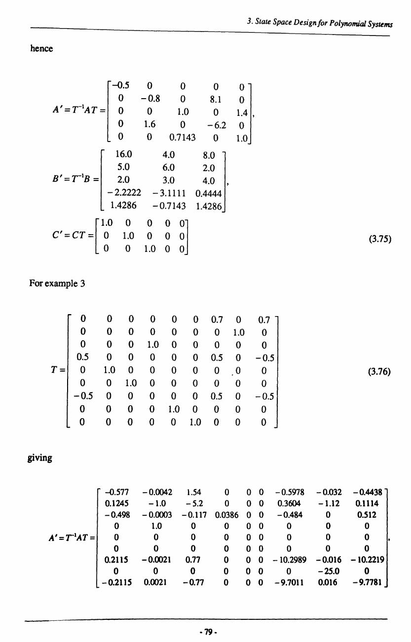
3. Slale Space Design/or Polynomial Systems
hence
-0.5 0 0 0 0 0 -0.8 0 8.1 0
A'=T-1AT= 0 0 1.0 0 1.4 , 0 1.6 0 -6.2 0 0 0 0.7143 0 1.0
16.0 4.0 8.0 5.0 6.0 2.0
B'=T-1B = 2.0 3.0 4.0 -2.2222 -3.1111 0.4444 1.4286 -0.7143 1.4286
[1.0 0 0 0
~J C'=CT= ~ 1.0 0 0 (3.75) 0 1.0 0
For example 3
0 0 0 0 0 0 0.7 0 0.7 0 0 0 0 0 0 0 1.0 0 0 0 0 1.0 0 0 0 0 0
0.5 0 0 0 0 0 0.5 0 -0.5 T= 0 1.0 0 0 0 0 0 0 0 (3.76)
0 0 1.0 0 0 0 0 0 0 -0.5 0 0 0 0 0 0.5 0 -0.5
0 0 0 0 1.0 0 0 0 0 0 0 0 0 0 1.0 0 0 0
giving
-f). 577 -0.0042 1.54 0 0 0 -0.5978 -0.032 -0.4438 0.1245 -1.0 -5.2 0 0 0 0.3604 -1.12 0.1114 -0.498 -0.0003 -0.117 0.0386 0 0 -0.484 0 0.512
0 1.0 0 0 0 0 0 0 0 A'=r1AT= 0 0 0 0 0 0 0 0 0
0 0 0 0 0 0 0 0 0 0.2115 -0.0021 0.77 0 0 0 -10.2989 -0.016 -10.2219
0 0 0 0 0 0 0 -25.0 0 -0.2115 0.0021 -0.77 0 0 0 -9.7011 0.016 -9.7781
·79·

3. Slale Space Design for Polynomial Sys~ms
0 0 0 0 0 0 0 0 0 0 0 0 0 0 0 0
B'=r1B = 0 0 1.0 0 0 0 0 1.0
14.2857 0 0 0 0 25.0 0 0
14.2857 0 0 0
1.0 0 0 0 0 0 0 0 0 0 1.0 0 0 0 0 0 0 0
C'=CT = 0 0 1.0 0 0 0 0 0 0 0 0 0 1.0 0 0 0 0 0 (3.77)
0 0 0 0 1.0 0 0 0 0 0 0 0 0 0 1.0 0 0 0
and for example 4
0 -1.0 1.0 0
T= 1.0 1.0 -1.0 -1.0 0 1.0 0 0 (3.78)
0 0 0 1.0
which gives
1.0 2.0 0 1.0 1.0 2.0
A'=T-1AT= 0 1.0 0 0 B'=T-1B = 1.0 1.0
0 1.0 1.0 1.0 ' 2.0 1.0 ' 0 1.0 0 1.0 0 1.0
[1.0 0 0
~] C'=CT= ~ 1.0 0 (3.79) 0 1.0
3.4.4 Results for the Method of Fahmy and O'Reilly
In each example the free parameters L in eqn (3.37) were chosen randomly
·80·

3. State Space Design/or Polynomial Systems
Example 1
The output feedback matrix
K = [-62.3913 89.0 ] , - 105.0 159.0
was obtained which placed the closed-loop eigenvalues at
-9.99999999997717
-9.00000000003750
-7.99999999998551
Example 2
The output feedback matrix
[
7.0749 - 3.2769 - 23.9639J K, = 7.5643 - 3.5401 - 25.5432
-1.9588 1.5799 5.1844
was obtained which placed the closed-loop eigenvalues at
-5.00000000000000 + j 4.99999999999994
-3.00000000000041
-1.99999999999951
-1.000000000000 16
Example 3
The output feedback matrix
3.1412 -0.5958 0.8563 0.2503 0.5197 -0.2009 24.2762 7.4052
K= 6.6958 9.9175 -143.9334 -14.7714
, 32.3750 46.0288 -698.4580 -63.5818
was obtained which placed the closed-loop eigenvalues at
- 81 -
(3.80)
(3.81)
5.7946 -0.7882 31.2904 -4.6199
-143.9688 18.0386 -693.0210 79.0398
(3.82)

3. Slale Space Design/or Polynomial Systems
-1.49999999999999 + j 1.49999999999999
-2.00000000000000 ± j 0.99999999999998
-16.99999999999997
-21. 99999999999998
-0.70000000000001
-29.99999999999999
-35.00000000000068
Example 4
The output feedback matrix
K =[ -30.5551 y -52.9081
- 66.3419
- 116.9301 81.4301 ] 143.7831
was obtained which placed the closed-loop eigenvalues at
-1.00000000000235 + j0.49999999999770
-4.00000000001050
-2. 99999999998448
3.4.5 Results for the Method of Daley
Again the free parameters were chosen randomly for each example
Example 1
(3.83)
With the a's in S, which are arbitrary, set to 1, the following output feedback matrix was
obtained
_[-10.9141 Ky - -105.0
88.9999 ] 1560.3744
which placed the closed-loop eigenvalues at
-10.00000000506724
-8.99999998539417
_8.00000000995767
(3.84)

3. Slale Space Design/or Polynomial Systems
and with the a's chosen randomly as
a 12] = [0.0500 0.7615]
the output feedback matrix was
K =[79.2752 y -105.0
89.0 ] -111.6407
giving the closed-loop eigenvalues at
-9.99999999983979
-9.00000000027615
-7.99999999988574
Example 2
(3.85)
(3.86)
With the a's setto 1, Vll was singular and so it was not possible to obtain a solution. However,
selecting them randomly as
a 13] = [0.7702 0.7702 0.8278] ~3 0.1253 0.1253 0.0159
(3.87)
gave a non-singular VII and thus a solution. Note that the second column is the same as the
fmt, this is due to the second column of ~ being the complex conjugate of the fmt. Also it
appears that any set of randomly chosen a's gave rise to a solution.
The output feedback matrix
[
0.6111
K, = 2.8451 -0.3818
-1.2109 - 3.5558 -0.1552
1.3832 ] 0.9548
-1.6337
was obtained which placed the closed-loop eigenvalues at
- 83-
(3.88)
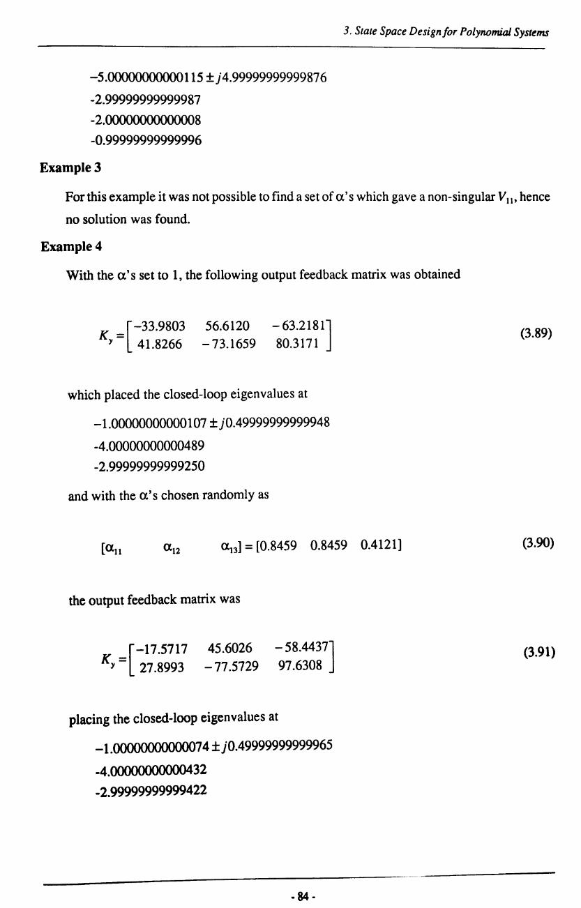
3. Slale Space Design/or Polynomial Systems
-5.00000000000 115 + j 4.9999999999987 6
-2.99999999999987
-2.00000000000008
-0.99999999999996
Example 3
For this example it was not possible to find a set of a's which gave a non-singular VII' hence
no solution was found.
Example 4
With the a's set to 1, the following output feedback matrix was obtained
K =[-33.9803 56.6120 -63.2181] y 41.8266 -73.1659 80.3171
which placed the closed-loop eigenvalues at
-1.00000000000107 + jO.49999999999948
-4.00000000000489
-2.99999999999250
and with the a's chosen randomly as
an] = [0.8459 0.8459 0.4121]
the output feedback matrix was
[-17.5717
K, = 27.8993 45.6026 - 58.4437]
- 77.5729 97.6308
placing the closed-loop eigenvalues at
-1.00000000000074 ± jO.49999999999965
-4.0Q000000000432
-2.99999999999422
- 84-
(3.89)
(3.90)
(3.91)

3. Slale Space Design/or Polynomial Systems
3.4.6 Discussion of the Results
Clearly the results show that the numerical properties of both methods are quite good with
the closed-loop eigenvalues being placed extremely accurately.
The method of Fahmy and O'Reilly (1988a) was able to find a solution which gave a
non-singular matrix of right eigenvectors for all the examples. However the method of Daley
(1990) has some difficulty in obtaining a non-singular sub-block of the matrix of right eigen
vectors in all cases. The rather unsatisfactory step of randomly selecting arbitrary scalars has to
be done in example 2 in order for a solution to be obtained. For example 3 no solution was
obtained at all.
The main problem with the method of Daley (1990) is clearly that of ensuring the
invertibility of VII'
This could be overcome by defining a vector sub-space that r must lie in such that Vn is
invertible. r could then be selected from the intersection of this space and the null space of ~,
which is a requirement for non-trivial solutions to equation (3.65).
For V~II to exist, its columns must be linearly independent, i.e
(3.92)
for all COj where at least one is non-zero. Note that yJI denotes the i'th column vector of Vn'
Writing this equation in vector form
(3.93)
From equation (3.60)
(3.94)
Therefore
[SJI ... S,t,] [COl' •• co,t ~ 0 (3.95)
- 85-

3. Slale Space Design/or Polynomial Systems
where Sj = [(A;I-ArIB],. This can be expressed in a more compact form
(3.96)
where
~. = [SI ' , ,S,] and r' = [roLli, . ,ro,t{ (3.97)
Equation (3.96) is clearly of the standard form Ax = b. For the case when b = 0 it is well - - -known that the set of solutions will form a basis of a vector subspace, generally known as the
null space of A. However, the case of b * 0 is of interest here and all that can now be stated is
that the set of solutions will lie in some vector subspace but that they may not necessarily fonn
a basis of that space.
For equation (3.96) this makes it difficult to define the set of possible r' vectors. It is
possible to investigate this subspace further which may possibly lead to a way of defining the
set of solution vectors to equation (3.96), However, a more significant problem remains, namely
that of the arbitrary scalar weights. Recalling that equation (3.92) must be valid for all ~
(i = 1 ~ r), where at least one is non-zero, it is clear that even if the set of r' vectors could be
found it would be extremely difficult to deduce the set of FI vectors using the fonn of r' in
equation (3.97). No solution to this problem was found and so the idea of obtaining a set of FI
vectors such that Vll is non-singular was not pursued further. It should be noted, however, that
the problem of a singular Vll only caused problems occasionally and did not prevent the appli
cation of the method in most cases.
A second possible problem is in the determination of a space for the FI vectors such that
there are non-trivial solutions to equation (3.65). The linear independence identity is used to
ensure the dependence of a set of vectors, the columns of[/-FI V1N(A/-ArIB],]. The only
condition for dependence is that at least one set of scalar weightings (one or more non-zero)
exists such that the weighted sum of the vectors is zero. This can be achieved by selecting a set
and forcing the sum to be zero, hence the reason that the FI vectors must lie in a null space.
Oearly this is actually selecting a subspace of the total space that the FI vectors may be in. This
subspace may not necessarily include a set of FI vectors that yield a non-singular VII'
- 86-

3. State Space Design/or Polynomial Systems
3.5 Summary
This chapter has outlined the transformation of the polynomial system to state space form
and detailed the interpretation of the output feedback matrix in terms of controller polynomials.
Due to the importance of the eigenvalues and eigenvectors in determining the shape of the
transient response it has been suggested that parametric methods be used to design the state space
controller.
Two approaches to the problem of parametric output feedback design have been investi
gated and their performance assessed when applied to a number of design examples.
The method of Fahmy and O'Reilly (1988a) is a multi-stage design where successive
output feedback loops are applied until the whole eigenstructure is assigned. It can be argued
that this gives the method greater flexibility and a wider set of possible feedback matrices.
However, it is difficult to know how to split the set of desired closed-loop eigenvalues. Good
solutions were obtained for all the examples considered.
The second method, Daley (1990), can be thought of as a parametric state feedback design
where the free parameters are constrained to effectively give output feedback. Problems arise
when dealing with these constraints. It is necessary to ensure the invertibility of a sub-block of
the matrix of right eigenvectors, which appears to be quite difficult for examples 2 and 3. By
randomly selecting some arbitrary scalars in the design process it was possible to obtain a solution
for example 2. However, this is an unsatisfactory way of approaching the problem as potentially
many random choices may have to be made in order to find a solution.
The results of the comparison show that both methods appear to have good numerical
properties, but the method of Daley (1990) did experience a number of difficulties. Although
this does not stop the method being used it does suggest that the method of Fahmy and O'Reilly
(1988a) would be more suitable. However when applied to a transformed polynomial system
the method of Fahmy and O'Reilly (1988a) failed to find a solution at all. The reasons for this
failure appear to be linked to the structure of the open-loop system matrices and a more detailed
discussion is included in chapter five where the robust design is applied to an example.
As mentioned in the introduction there are a number of options when considering the state
space design. In the area of eigenstructure assignment techniques a number of interesting methods
have recently been proposed, unfortunately too late for consideration in this work.
Burrows and Patton (1988, 1989a, 1989b, 1990a, 1990b) have carried out much work in
the area of robust eigenstructure assignment, utilising numerical minimisation methods to select
appropriate sets of eigenvectors from prespecified regions of the complex plane on the basis of
a number of robustness measures, including low norm control law and maximally orthogonal
- 87-

3. State Space Design for Polynomial Systems
eigenvectors. White (1991) has proposed a scheme which appears to be as numerically stable as
Fahmy and O'Reilly (1988a) but which overcomes the problem of protection by assigning the
desired eigenstIUcture in just one stage.
It would certainly be interesting to investigate these methods further and assess their impact
on the robustness of the polynomial system. However, it is worth reiterating at this stage that
any effective robust state space design procedure could be used as the aim is to illustrate and
prove the concept of designing a polynomial controller via the state space domain.
The overall conclusion of this chapter is that the method of Daley (1990) is to be used as
the basis of the state space design, which is assumed in all of the following chapters.
- 88-

3. State Space Designfor Polynomial Systems
REFERENCES
Brasch, F.M., and Pearson, J .B. (1970)
'Pole Placement using Dynamic Compensator'
IEEE Transactions on Automatic Control, vIS, pp 34-43
Burrows, S.P. (1990)
'Robust Control Design Techniques using Eigenstructure Assignment'
PhD Thesis. Dept of Electronics. University of York, U.K.
Burrows, S.P. and Patton, RJ. (1988)
'Robust Eigenstructure Assignment using the CTRL-C Design Package'
Sixth International Conference on Systems Engineering. Coventry, U.K., pp 868-875
Burrows, S.P. and Patton, RJ. (1989a) 'On Robustness Properties of Eigenstructure Assignment in the Control of Multivariable Uncertain Systems'
Sixth IFAC Symposium on Dynamic Modelling and Control of National Economies, Edinburgh, U.K.,
v2,pp513-517
Burrows, S.P. and Patton, R.J. (1989b) 'Robust Eigenstructure Assignment for Flight Control using the CTRL-C Design Package' A1AA Conference on Guidance, Navigation and Control, Boston, Mass, U.S.A., v2, pp 1489-1494
Burrows, S.P. and Patton, R.J. (1990a) 'Optimal Eigenstructure Assignment for Multiple Design Objectives'
1990 American Control Conference, San Diego, California, U.S.A., pp 1978-1683
Burrows, S.P. and Patton, R.J. (1990b) 'Robust Low Norm Output Feedback Design for Flight Control Systems'
A1AA Conference on Guidance, Navigation and Control, Boston, Mass, U.S.A.
Daley, S. (1990) 'On Eigenstructure Assignability using parametric output feedback'
Brunei University Control Engineering Centre Internal Report, August 1990
Fahmy, M.M. and O'Reilly, 1. (1988a) 'Multistage Parametric Eigenstructure Assignment by Output Feedback Control'
International Journal of Control, v48, nl, pp 97-116
Fahmy, M.M. and O'Reilly, J. (1988b) 'Parametric Eigenstructure Assignment by Output Feedback Control: The Case of Multiple Eigenvalues'
International Journal ofConlrol, v48, n4, pp 1519-1535
Friedland, B. (1986) 'Control System Design - An Introduction to State Space Methods'
McGraw Hill, London. U.K.
Kallath, T. (1980)
'Linear Systems'
Prentice Hall. London. U.K.
Kalsi. R.S. (1991) • A Multi-Stage Parametric Approach to Output Feedback Controller Design'
Final Year Project. Dept ofElec Eng. Brunei University. Middlesex. UX.
- 89-

~ura.}{. (1975)
'Pole Assignment by Gain Output Feedback'
IEEE Transactions on Automatic Control, v20, n4, pp 509-516
Ogata. K. (1987)
'Discrete Time Control Systems'
Prentice Hall, London, UK.
Roppenecker, G. and O'Reilly, J. (1989)
'Parametric Output Feedback Controller Design' Automatica, v25, n2, pp 259-265
Sobel, K.M. and Shapiro, E. Y. (1985)
3. Slate Space Designfor Polynomial Systems
'Eigenstructure Assignment: A Tutorial - Part II Applications'
Proceedings of the 1985 American Control Conference, vI, pp 461-467 IEEE, New York, U.S.A. (Cat No. 85CH2119-6)
Srinathkumar, S. (1978) 'Eigenvalue!Eigenvector Assignment Using Output Feedback'
IEEE Transactions on Automatic Control, v23, nl, pp 79-81
Topaloglu, T. and Seborg, D.E. (1975) 'A Design Procedure for Pole Assignment using Output Feedback'
International Journal of Control, v22, n6, pp 741-748
White, B.A. (1991)
'Eigenstructure Assignment by Output Feedback' International Journal of Control, v53, n6, pp 1413-1429
-90 -
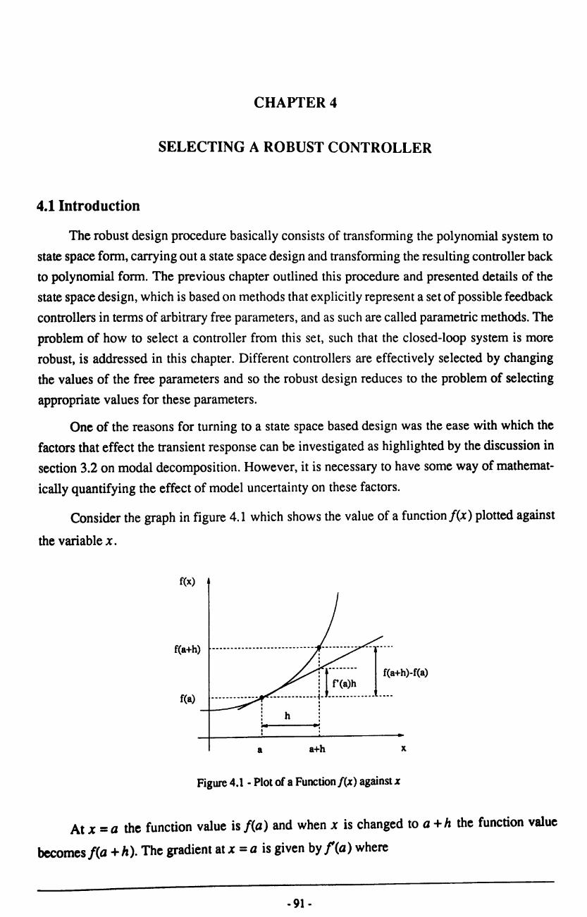
CHAPTER 4
SELECTING A ROBUST CONTROLLER
4.1 Introduction
The robust design procedure basically consists of transfonning the polynomial system to
state space form, carrying out a state space design and transforming the resulting controller back
to polynomial form. The previous chapter outlined this procedure and presented details of the
state space design, which is based on methods that explicitly represent a set of possible feedback
controllers in terms of arbitrary free parameters, and as such are called parametric methods. The
problem of how to select a controller from this set, such that the closed-loop system is more
robust, is addressed in this chapter. Different controllers are effectively selected by changing
the values of the free parameters and so the robust design reduces to the problem of selecting
appropriate values for these parameters.
One of the reasons for turning to a state space based design was the ease with which the
factors that effect the transient response can be investigated as highlighted by the discussion in
section 3.2 on modal decomposition. However, it is necessary to have some way of mathemat
ically quantifying the effect of model uncertainty on these factors.
Consider the graph in figure 4.1 which shows the value of a function I(x) plotted against
the variable x.
f(x)
f(a+h)
f(a)
--------------.--.-----.--.- --.-----.- --r-'-' · , , · : --.----- f(a+h)-f(a) : r(a)h .............•. 1 ................ .
. h , :. I I
a
, ,
· .' , · a+h x
Figure 4.1 - Plot of a Function I(x) against x
At X = a the function value is f(a) and when x is changed to a + h the function value
becomes f(a + h). The gradient at x = a is given by f(a) where
- 91 -

4. Selecting a Robust Controller
(4.1)
I(a + h) - I(a) is called the increment (of I(x) from x = a to x = a + h) and is denoted by
AI
AI = I(a + h) - I(a) (4.2)
r(a)h is called the differential (at x = a with increment h) and is denoted by dl
dl=r(a)h (4.3)
The differential is also sometimes referred to as the sensitivity, denoting that the expression
evaluates how sensitive the function is to changes in the variables.
The increment is the actual change in the function due to a change in the variable whereas
the differential is an estimate of the change in the function. The differential hence fonns the
basic mathematical tool needed to estimate the change in the factors that affect the transient
response due to a change in the model parameters. Further information on differential calculus
can be found in Salas and Hille (1990).
It is now possible to define a function consisting of expressions for the differentials of the
factors of interest. This function is often referred to as a cost function, an objective function or
a performance index. As it effectively represents the sensitivity to model uncertainty, it is
desirable to obtain the lowest possible value for the function, which has clearly reduced the
robust design to an optimisation problem as desired.
With complicated functions, as is the case here, there may be many local minima, at which
the function has the lowest value with respect to the neigh bourhood of possible points. The lowest
local minimum is called the global minimum and clearly the ultimate goal of any optimisation
procedure is to find this point. For complicated functions this represents an extremely difficult
task and a more realistic target would simply be to aim for a good local minimum point which
yields the desired level of improvement.
Having established how to quantify the effect of model uncertainty, the next section
considers the problem of defining appropriate cost functions. Following this is a more detailed
discussion of numerical optimisation which helps to classify the problem being considered
allowing the selection of the most suitable optimisation algorithm.
-92-

4. Selecting a Robust Controller
4.2 Cost Functions
The previous chapter illustrated, through modal decomposition, how important the
eigenvalues and eigenvectors are in determining the shape of the transient response. The way
these factors are affected by structured model uncertainty will directly determine how the
transient response is affected. This opens up a number of possibilities for evaluating performance
robustness. Gourishankar and Ramar (1976), Owens (1988) and Owens and O'Reilly (1989) use
eigenvalue sensitivity as the basis on which to select robust controllers. The sensitivity of the
whole eigenstructure (eigenvalues and eigenvectors) is the approach used by Crossley and Porter
(1969), Ling and Wang (1988). Other authors have investigated alternative approaches such as
the conditioning of the matrix of right eigenvectors, V, which is claimed to improve the sensitivity
of the transient response (Kautsky, Nichols and Van Dooren, 1985; Byers and Nash, 1989;
Owens, 1991b). The cost function in this case should descIibe the change in the output of the
system due to a change in some or all of the model parameters.
Before considering the details of some alternative cost functions it is necessary to quantify
the error in the state space model. Chapter 3 described how the polynomial system is transformed
to a state space system. From this it is clearly unnecessary to consider errors in the C matrix, as
all its elements will be constant, hence the model uncertainty can be represented as
A =Ao+M
B = Bo + till
(4.4)
(4.5)
where M and till are the increments of A and B defined as
u
M = LPlt, (4.6) , = 1
u
till = L Q,t, (4.7) , = 1
P, and Q, represent the known infomlation about the structure of the errors and t, the
unknown magnitude of the errors. The increments can be approximated by the differentials
dA=M
dB = till
- 93 -
(4.8)
(4.9)
------------------
4. Selecting a Robust Controller
where
(4.10)
(4.11)
and t£, is the change (or increment) in E. Clearly the partial derivatives are
aA =p aE, ' (4.12)
aB aEt = Q, (4.13)
assuming the E,'S are independent.
4.2.1 Eigenvalue Differential Cost Function
A number of authors have derived expressions for eigenvalue sensitivity, for example
Crossley and Porter (1969), Ling and Wang (1988), Skelton (1988). In general all such
expressions are derived from the equation
A v· =A.V. c~ ,~ (4.14)
where Ac denotes the closed-loop system matrix, ~ and Yi its associated eigenvalues and right
eigenvectors respectively. Similarly for the left eigenvectors,!f;
(4.15)
Following Porter and Crossley (1972), partially differentiating (4.14) with respect to e. gives
-94 -
4. Selecting a Robust Controller
(4.16)
Pre-multiplying by !!i
(4.17)
From (4.15)
(4.18)
Which means that
(4.19)
Hence (4.17) becomes
(4.20)
For normalised eigenvectors !0" Yi = 1, hence
(4.21)
Also as Ac =A +BKC
- 95-

4. Selecling a Robusl COnlTolkr
dAc d(A + BKC) dA dB -= =-+-KC dE, dE, dE, dE,
=P,+Q,KC (4.22)
Hence
d~ T dE, =}f; (P, + Q,KC)Y.,; (4.23)
and the eigenvalue differential can then be expressed as
(4.24)
where dAi' denotes the differential of the i'th eigenvalue to the t'th error. As already stated the
aim is to determine the value of the free parameters which yield the lowest value for this function.
However the function is comprised of two parts, the known d'A./iJE, and the unknown flE.,. As
there is no control over the value of .1£" the cost function should only consist of the known partial
derivative part, giving the eigenvalue differential cost function as
U IJ (dA.)2 1 =11 = 1: .1: ~i' -'
,= 1, = 1 dE, (4.25)
The partial derivative is squared to ensure that the cost function remains positive. ~il are
positive weights used to place importance on each of the eigenvalues.
4.2.2 Eigenstructure Differential Cost Function
The previous section evaluated an expression for the eigenvalue differential, however from
the modal decomposition it is clear that the differential of the whole eigenstructure (eigenvalues
and eigenvectors) should be considered. This has also been dealt with by a number of authors,
for example Crossley and Porter (1969), Porter and Crossley (1972), Ling and Wang (1988) and
again are generally derived from equations (4.14) and (4.15). However, for the parametric method
the right eigenvectors are expressed as
- 96·

4. Selecting a Robust Controller
(4.26)
which can be used to evaluate an expression for the eigenvector differential. Partially differentiating (4.26) gives
avo dO .. .J -Arl diD -== ' BL+(A.J -Arl-D L dE, dE, 'dE,
(4.27)
Substituting dA/dE, from (4.23) gives
As W = V-I, where W is the matrix of left eigenrows and V is the matrix of right eigen
vectors, it is relatively simple to find an expression for the partial derivative of the left eigenrows.
dWT dfeTV-I) dV dV -==!...= ~ =-e~V-I-V-1 =-e~W-W dE, de, ~ dE, ~ dE, (4.29)
where ~ is the i'th column of the unit matrix.
The right eigenvector differential can then be expressed as
dy;, = (-(Ai - A rl <!i (P, + Q,KC )y;1 - P,) (Ai - A riB L + (/...;1 - A r1QiJ)AE"
(4.30)
where dl!;, denotes the differential of the j'th right eigenvector to the t'th error. Similarly the left
eigenrow differential is
·97 •

d T T av w· =-e·W-W~ ~, ~ aE, '
4. Selecting a Robust COnlToller
(4.31)
The differentials are vector values and as with the eigenvalue differential consist of a
known and unknown part. Using only the known partial derivative part and ensuring that the
cost function is a positive scalar value gives the eigenstructure differential cost function as
(4.32)
where 11·11 denotes any vector norm, and Tlil are positive weights. As itis necessary to also consider
the eigenvalue differential to ensure the eigenvalue sensitivities do not become too large, the
overall cost function will be
(4.33)
where 0' is also a positive weight.
4.2.3 Transient Response Differential Cost Function
The previous cost functions merely consisted of expressions for the eigenvalue and
eigenvector sensitivities, as it is known that they are important in determining the sensitivity of
the transient response. However, as an expression for the transient response was actually derived
in chapter 3, it would be interesting to directly determine its differential and hopefully define a
transient response differential cost function. It should be noted that other authors have also looked
at this problem, for example Skelton (1988) defines an expression for output sensitivity by
differentiating the state equations.
The differential of the transient response is given by
d (k) = ay(k) & y aE, I
(4.34)
and from chapter 3
- 98-

4. Selecting a Robust Controller
(4.35)
hence the partial derivative is
ay(k) " avoW!( k-l ) a = CoL a~ A~X(O)+ L A~-j-lBuU) e, ,=1 e, j=O
(4.36)
which gives
ay(k) " avow!( k-l ) -=--=C oL ~~ A~X(O)+ L A~-j-lBuU) + ae, , = 1 ae, j = 0
VoW~ kA~-l_' x(O)+ L (k - . -1)A~-j-2-' BUU')+A~-j-l-UU) ( aAo k - l( aAo alJJ))
~~ , ae, - j = 0 J , ae, - , ae, -
(4.37)
This is quite a complicated expression, the evaluation of which is dependent on particular
values of k, the discrete time sequence. It is clearly not very useful as regards defining a cost
function, however upon closer examination it can be seen that the eigenvectors of the system
always appear in the form of ~~. This does suggest that a more suitable representation of the
eigenvector differential would be obtained by considering the term ~~.
Partially differentiating this term gives
(4.38)
and the transient response differential cost function can be defined as
(4.39)
where
----------------------- --~---~----------
- 99-
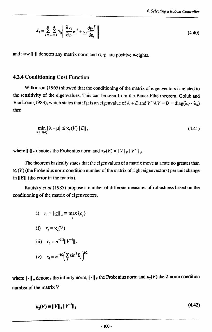
4. Selecting a Robust Controller
J ~~ ~T a!!l 3= ~ ~Yit -a ~ +Yi-a 1=li=1 ~ ~
(4.40)
and now 11·11 denotes any matrix norm and 0, Yit are positive weights.
4.2.4 Conditioning Cost Function
Wilkinson (1965) showed that the conditioning of the matrix of eigenvectors is related to
the sensitivity of the eigenvalues. This can be seen from the Bauer-Fike theorem, Golub and
Van Loan (1983), which states that if /..l is an eigenvalue of A + E and V-I A V = D = diag(A.1••• A./l)
then
(4.41)
where 11·11 F denotes the Frobenius norm and KF(V) = II VII F II V-III F'
The theorem basically states that the eigenvalues of a matrix move at a rate no greater than
Kp(V) (the Frobenius norm condition number of the matrix of right eigenvectors) per unit change
in II Ell (the error in the matrix).
Kautsky et al (1985) propose a number of different measures of robustness based on the
conditioning of the matrix of eigenvectors.
i) '1 = II cll_ = m~x{c) J
ii) '2 = ~(V)
iii) '3 = n -11211 v-III F
iv) '4 = n-lirSin29j JI2
where n . II. denotes the infinity norm, II· II F the Frobenius norm and K2(V) the 2-nonn condition
number of the matrix V
1C2(V) = I Va 2 n y-1U 2 (4.42)
- 100-

4. Selecting a Robust Controller
c = [C.,· . ·clt ] is the vector of condition numbers, which assuming that the right eigenvectors are
normalised such that II £; 112 = 1, are defined as
Ci = 1I~1I2 (4.43)
and lastly OJ are the angles between the eigenvectors v j and certain corresponding orthononnal
vectors v .. ~
All these measures attain their minimum simultaneously when the assigned eigenvalues
are as insensitive as possible. Kautsky et al (1985) go on to propose two further weighted measures
(L d~ sin2 e .)1/2 . J J
vi) '4(D) = J (Ld~)112 . J )
J
A suitable set of weights is given by dt = (1 -I Ajl ) for the discrete time case. Using these
weights has the effect of minimising an upper bound on the stability margin of the closed-loop
system.
Byers and Nash (1989) also propose a number of measures of robustness
vii) 's = ~[V]
viii) -1
'6=-'s
ix) 212 '7 = II VII F + II V- II F
-1 x) '8=-'7 xi) '9 = log['7]
- 101 -

4. Selecting a Robust Controller
and state that although no cost function is unifonnly better than the others, functions rg and r9
generally perfonn well. r9 is recommended for general use, particularly if ill-conditioned
problems are to be encountered. However, a recent paper, Owens (1991a) suggests that r9 may not be effective in certain cases.
From the literature it is certainly very difficult to judge the suitability of any particular
conditioning based cost function. Owens ( 1991 b) does discuss a number of the possible functions
and gives some insight into their relative benefits. From this and remembering the Bauer-Fike
theorem, a good initial choice would seem to be
(4.44)
Owens (1991b) also reports that considering (KF(V»2 resulted in a faster convergence to
the solution for the example considered.
4.3 Optimisation Techniques
The Numerical Algorithms Group (NAG) library of FORTRAN 77 routines contains a
number of quite sophisticated optimisation algorithms. It was felt that using the routines in this
library would greatly simplify the implementation of the robust design method and further details
of the reasons for this decision can be found in the following chapter.
The aim of this section is to introduce the concepts behind numerical optimisation and
some of the tenninology used. This will then allow the problem being considered to be classified
which will aid in the selection of an appropriate optimisation routine. The section finishes with
a brief introduction to some of the main types of algorithms. Because the NAG routines are to
be used the following is biased to their approach and is largely taken from NAG (1990).
4.3.1 Introduction and Terminology
The solution of optimisation problems by a single, all-purpose, method can be cumbersome
and inefficient. For this reason such problems are classified into particular categories for which
various algorithms are best suited. The problem can be characterised by the properties of the
cost function and the constraint functions, for example
-102 -

Properties of cost Function
Nonlinear
Sums of squares of nonlinear functions
Quadratic
Sums of squares of linear functions
Linear
Properties of Constraints
Nonlinear
Sparse linear
Linear
Bounds
None
4. Selecting a Robust Controller
It is necessary to express these types of problems mathematically for numerical optimi
sation. Firstly, consider unconstrained problems where there are no restrictions on the value of
the variables. Mathematically the problem can be stated as
minimise F C!.) :!
where x E Ria are the variables and F C!.) the function.
(4.45)
The NAG library makes special provision for problems which can be expressed as the sum
of squared functions, often referred to as a least squares problem. The mathematical statement
of this problem is
minimise {f[=i~/~} (4.46)
where the i'th element of the m-vector [is the function h<!), which is often referred to as a
residual.
Now consider the problem subject to constraints of some kind. As indicated above there
are a number of categories of constraints, probably the most straightforward of which are bounds
on the variables. For the problem of (4.45) the variables can be bounded by
(4.47)
- 103-

4. Selecting a Robust Controller
where X; are the respective elements of the vector X and I; the lower bounds and Ui the upper
bounds on the value of Xi' This does assume that bounds exist on all the variables, but by allowing
u; = 00 and Ii = -00 all the variables need not be restricted.
Next consider linear constraints, which are defined as linear functions in more than one
of the variables, e.g. 3x1 + 2x2 ~ 4. Mathematically such constraints can be described by
Equality constraints a?'x =b· =.J _ J i = 1,2", ',ml
Inequality constraints fi'x ~ b; i =m1 + 1", ',~ fi' x '5: b; i = m2 + 1" . . ,Tn]
Range constraints T i =m3+ 1", ',m4 s·<a·x<t-)-=.J_-)
j = 1", ',m4 -m3
Bound constraints [. <x· < u· ,- ,- J i=12···n " ,
where each f!; is a vector of length nand bj , Sj and tj are constant scalars. Also note that any of
the categories above may be null.
If F C!.) is a linear function, the linearly constrained problem is termed a linear programming
problem and if F C!.) is a quadratic function, the problem is termed a quadratic programming
problem.
Lastly, in the discussion of the characterisation of the problem, consider the case of (4.45)
subject to nonlinear constraints, e.g. x~ + X3 ~ O. The above mathematical description of the linear
constraints still applies but now the following constraints must also be considered
Equality constraints i = 1,2,· . ',ms
Inequality constraints i =ms+ 1,·· ',""
Range constraints i ="" + 1" . ',"", j = 1,2,·· ',m,-""
where each c; is a nonlinear function and Vj' Wj are constant scalars. Again any category may be
null.
·104 •

4. Selecting a Robust Controller
The problem facing the optimisation algorithms is to find a minimum of the given function
F(!J subject to constraints of one of the above types. It is worth mentioning here that the function
is likely to have many minima, each called a local minimum because the function has the lowest
value at that point with respect to the neighbourhood of possible points. The lowest of these local
minima is termed the global minimum for obvious reasons. In the face of this, all that can be
expected of the algorithms is that they find a local minimum point, and by starting the algorithm
in a number of places it is hoped to find a local minimum that yields a desirable result.
For an algorithm to find a minimum point (either local or global) it must have some way
of determining whether or not a particular point is a minimum. Also it must have a method of
determining the direction to move, such that a minimum point can be found. The next part of
this discussion attempts to address this point by first reviewing some of the required mathematics
and defining conditions for a minimum.
The vector of first partial derivatives of F~) is called the gradient vector and is denoted
by g C!.), i.e.
[ aF C!.) aF~) aF ~)]T
g C!.) = a ' a , ... , a Xl X2 Xn
(4.48)
The gradient vector is of importance in optimisation because it must be zero at an
unconstrained minimum of any function with continuous first derivatives.
The matrix of second partial derivatives of the function is termed its Hessian matrix and
is denoted by G ~). Its (i ,j)'th element is given by
(4.49)
If F~) has continuous second partial derivatives then G~) must be positive semi-definite
at any unconstrained minimum of the function.
In nonlinear least squares problems, the matrix of first derivatives of the vector valued
function [is termed the Jacobian matrix.
- 105 -

4. Selecting a Robust Controller
4.3.2 Classification of the Problem
At this stage it is possible to determine which category the problem of interest lies in. To
do this it is necessary to first of all examine the cost functions being considered. The variables
are obviously the free parameter vectors used to determine the eigenvectors and hence the output feedback matrix.
Consider the relationship between the variables which are the free parameter vectors i, introduced by the parametric design approach, and the value of the function, which is made up
of terms dependent on the closed-loop eigenvalues and eigenvectors. The relationship is clearly
a very complicated one and it is not a straightforward task to determine the character of it. The closed-loop system matrix is given by
(4.50)
for state feedback. Consider the expression for the state feedback matrix
(4.51)
and the expression for the right eigenvectors
(4.52)
where the definition of the terms involved can be found in chapter 3, which discusses the
parametric design methods in detail. Note that it was concluded in that chapter that the method
of Daley (1990) will form the basis of the state space design.
Because of the dependency of the right eigenvectors y; on the free parameter vectors t ,
nonlinear terms will be present in the evaluation of Kx. Hence the problem is of a nonlinear
nature.
Because the parametric design approach of Daley (1990) is forcing the state feedback
matrix to be in the form [K, : 0], such that output feedback can be used, the free parameter vectors
L are subject to constraints which from chapter 3 were shown to be
(4.53)
·106 -

4. Selecting a Robust Controller
Again because of the dependency of the eigenvectors on the free parameter vectors, this
equation is of a nonlinear nature. However Daley (1990) did reduce this constraint equation to
two further equations
(4.54)
(4.55)
This has not removed the non-linearity, but does give an indication of how the actual
constraints can effectively be removed. r contains all the free parameter vectors associated with
Fl which can be chosen freely provided that r lies in the null space of the matrix ~. Once Fl is
determined, the remaining free parameter vectors can be selected subject to equation (4.54). This
also requires the vectors to be selected from a null space. All the null spaces involved will have
a set of basis vectors, and any vector that lies in these null spaces will simply be a linear
combination of the basis vectors. For example consider a null space described by the set of basis
vectors
(4.56)
To select a vector y which lies in this null space, it must satisfy
(4.57)
where the scalar values, ~ are completely arbitrary.
This clearly demonstrates that to effectively remove the constraints from the problem, the
scalar multipliers of the basis vectors of the null spaces should be used as the free parameters.
If this approach is taken the robust design can then be classified as an unconstrained
nonlinear optimisation problem. Examining the eigenvalue differential cost function, I. it is
easily seen that it consists of the sum of a number of squared terms. This clearly fits into the
description of the least squares type of problem. However to gain any real benefit from the least
squares formulation in the NAG library it is necessary to ensure that the number of squued terms
is greater than the number of variables. The cost functions J2 and J, consist of a number of terms
·107·

4. Selecting a Robust Controller
which are norms of vectors or matrices. It is possible to force these into a least squares framework
by squaring the norms, but such a step would only really be necessary if computational efficiency
(the major advantage of the least squares framework) becomes critical.
4.3.3 Common Optimisation Methods
All the algorithms in the NAG library generate an iterative sequence x(k) that converges
to the solution x· in the limit. The sequence is usually constructed by satisfying
x(k + 1) =x(k)+a(k)p(k) (4.58)
where the vector p (k) is termed the direction of search and a(k) is the step length.
The step length is chosen such that FfJ..(k + 1» < FfJ..(k» and is computed by performing
a one-dimensional optimisation. The NAG library uses two techniques for one-dimensional
optimisation, one fits a quadratic polynomial using only function evaluations and the other uses
additional information about the gradient to fit a cubic polynomial.
The major differences between the various methods arise due to the need to use varying
levels of information about the derivatives of F fJ..) in defining the search direction, further details
can be found in Gill and Murray (1981). Four common algorithms for unconstrained minimisation
are
i) Newton-Type Methods (Modified Newton Methods)
Newton-type methods use the Hessian matrix GfJ..(k», or a finite difference
approximation to G fJ..(k », to define the search direction. Newton-type methods are
the most powerful methods available for general problems and will find the minimum
of a quadratic function in one iteration.
ii) Quasi-Newton Methods
Quasi-Newton methods approximate the Hessian G fJ..(k» by a matrix B (!(k» which
is modified at each iteration to include information obtained about the curvature of
FW along the latest search direction. Although not as robust as Newton-type
methods, quasi-Newton methods can be more efficient because G(!(k» is not
computed, or approximated by finite differences. Quasi-Newton methods minimise
a quadratic function in n iterations.
iii) Conjugate-Grtldient Methods
·108 •

4. Selecting a Robust Controller
Unlike Newton-type and quasi-Newton methods, conjugate gradient methods do not
require storage of an n by n matrix and so are ideally suited to solve large problems.
Conjugate-gradient type methods are not usually as reliable or efficient as
Newton-type, or quasi-Newton methods.
iv) Downhill Simplex Method
This method is due to NeIder and Mead (1965) and is a completely self-contained
approach that does not use one-dimensional minimisation, unlike the previous
methods. It requires only function evaluations, so no derivative information is
needed. The method is not very efficient in terms of the number of function evalu
ations that it requires but is numerically quite robust.
4.4 Summary
The previous chapter discussed the state space design where it was decided to use para
metric methods which explicitly represent a set of possible feedback controllers in terms of
arbitrary free parameters. This chapter has been concerned with the problem of selecting the free
parameters such that the resulting controller yields a closed-loop system with improved per
formance robustness.
To achieve this a suitable function relating the sensitivity of the closed-loop system to
structured model uncertainty can be defined, and the free parameters selected such that this
function is minimised. This has clearly reduced the robust design to an optimisation problem as
desired, which can then be solved using numerical methods. Of course it can only be expected
that a local minimum point is found and by starting the optimisation procedure from a number
of points it is hoped to find a local minimum which yields the desired level of robustness.
For performance robustness the effect of model uncertainty on the shape of the transient
response is of interest. Through modal decomposition it was shown that the sensitivity of the
transient response is strongly related to the sensitivity of the eigenvalues and eigenvectors,
leading to the definition of a number of cost functions. One further cost function was also included
which is based on the conditioning of the matrix of right eigenvectors.
Having established suitable cost functions, the fundamentals of numerical optimisation
were discussed in more detail, showing how problems can be categorised to help in the selection
of an appropriate optimisation algorithm. The problem being considered can be classified as an
unconstrained nonlinear problem, although for the design method of Daley (1990), some
re-arrangement of the problem had to be carried out. This involved re-defining the free parameters
to be scalar multipliers of the basis vectors of the null space of a matrix.
-109 -

REFERENCES Byers, R. and Nash, S.G. (1989)
, Approaches to Robust Pole Assignment'
International Journal ofConlrol, v49, nl, pp 97-117
Crossley, T.R. and Porter, B. (1969)
'Eigenvalue and Eigenvector Sensitivities in Linear Systems Theory'
International Journal ofConlrol, v 10, n2, pp 163-170
Daley, S. (1990)
'00 Eigenstructure Assignability using parametric output feedback'
Brunei University Control Engineering Centre Internal Report, August 1990
Gill,P.E. and Murray, W. (1981)
'Practical Optimization'
Academic Press, London, UK.
Golub, G.H. and Van Loan, C.F. (1983)
'Matrix Computations'
North Oxford Academic Publishing, Oxford, U.K.
Gourishankar, V. and Ramar, K. (1976)
4. Selecting a Robust Controller
'Pole Assignment with Minimum Eigenvalue Sensitivity to Plant Parameter Variations'
International Journal of Control, v23, n4, pp 493-504
Kautsky, J., Nichols, N.K. and Van Dooren, P. (1985)
'Robust Pole Assignment in Linear State Feedback'
International Journal of Control, v41, n5, pp 1129-1155
Ling, Y. and Wang, B. (1988)
'First and Second Order Eigensensitivities of Matrices with Distinct Eigenvalues'
International Journal of Systems Science, v19, n7, pp 1053-1067
NAG (1990)
'Fortran Library Manual Mk 14'
Numerical Algorithms Group Ltd, Oxford, U.K.
Neider, J .A. and Mead. R. (1965)
, A simplex Method for Function Minimisation'
Computer Journal, v7, pp 308-313
Owens, T.1. (1988)
'Parametric Output Feedback Control with Response Insensitivity'
International Journal o/Control, v48, n3, pp 1213-1239
Owens, T.1. and O'Reilly, J. (1989)
'Parametric State Feedback Control for Arbitrary Eigenvalue Assignment with Minimum Sensitivity'
lEE Proceedings, Pt D, v136, n6, pp 307-312
Owens, T.1. (1991a) , A Framework for Optimal Control by Nonlinear Programm ing'
International Symposium on Applied Mathemalical Programming and Modelling.
Brunei University, Middlesex. U X.
- 110-

4. Selecting a Robust Controller
Owens, T.J. (1991b)
'Parametric State Feedback Control for Arbitrary Eigenvalue Assignment with Minimum
Condition Number'
1991 European Control Conference. Grenoble. France. v2, pp 1292-1294
Hermes. Paris. France.
Porter, B. and Crossley, R. (1972)
'Modal Control, Theory and Applications'
Taylor and Francis Ltd. London. U.K.
Sallas, S.L. and Hille, E. (1990)
'Calculus - One Variable'
John Wiley and Sons. Chichester. U.K.
Skelton, R.E. (1988)
'Dynamic Systems Control'
John Wiley and Sons. Chichester. U.K.
Wilkinson, J.H. (1965)
'The Algebraic Eigenvalue Problem'
Clarendon Press. Oxford. U.K.
- 111 -

CHAPTERS
IMPLEMENTATION AND APPLICATION OF THE
ROBUST DESIGN PROCEDURE
S.1 Introduction
The problem being considered is that of designing a polynomial controller for a system in
input-output form, such that the closed-loop system is robust to changes in the parameters of the
plant being controlled. The preceding chapters have defined this problem and proposed a possible
approach to solving it, involving transforming to state space form and performing a parametric
output feedback design. The extra degrees of freedom in the design are then chosen to satisfy
some robustness criteria using the techniques of numerical optimisation.
There are still a number of unanswered questions though, involving the choice of cost
function and optimisation technique. General answers are not easily provided as to a certain
extent they are dependent on the actual plant being considered. To help illustrate how to make
suitable choices, the application of the proposed design method to an example is considered in
this chapter.
At this stage a secondary set of problems comes to light, namely those related to the
implementation of the method. This is an important aspect, as the way the method is implemented
will have a significant effect on its performance mainly in terms of speed. A discussion of the
major points regarding the implementation is presented which highlights the computational
requirements of the method as well as detailing some of the main problems encountered and
how they were overcome.
As previously mentioned in chapter three the state space parametric method of Fahmy and
O'Reilly (1988) experienced some difficulties when applied to transformed polynomial systems.
The problems encountered with this approach when applied to the example being considered
are also discussed in this chapter leading to the conclusion that the state space design should be
based on the parametric method of Daley (1990).
A comprehensive set of results is presented for each of the cost functions which aims at
highlighting how the weights are chosen and the typical improvement that can be achieved with
this approach. The chapter finishes with a discussion of these results and conclusions about the
performance of the proposed cost functions.
- 112-
5. Implementation and Application of the Robust Design Procedure
5.2 Implementation of the Robust Design Procedure
Pro-Matlab v3.5 is a very flexible interactive package that allows easy development of
ideas and designs. It contains a large number of quite complex in built functions largely relating
to matrix operations, such as inversion, singular value decomposition and factorisations. A
number of other functions for particular tasks are available through optional toolboxes, for
example in the areas of control system design and system identification. The package is installed
on a Sun 3/60 workstation running under the UNIX operating system in a windows environment.
To help illustrate the programs being used a number of flowcharts have been included
which can be found at the end of the chapter. Appendix B contains listings of the actual programs
for more detailed information.
Figure 5.1 outlines the overall design from specifying a polynomial system to obtaining
the robust controller polynomials. The loop is indicative of the optimisation procedure where a
local minimum value of the cost function is sought. Figure 5.2 expands on the parametric design
stage and as can be seen a significant level of computation is required for this part, which suggests
that it will largely determine the time taken to perform one iteration of the optimisation phase.
Such a design is very easy to implement in Pro-Matlab due to the number of inbuilt
functions. However Pro-Matlab only has the downhill simplex method of optimisation available I
which, although numerically robust, does not perform well on complex problems.
The Numerical Algorithms Group (NAG) library contains a number of routines for
numerical optimisation based on various algorithms, as outlined in chapter 4. The library routines
are however written in Fortran 77.
This suggests a number of possible options; 1) Perform the whole design in Pro-Matlab;
2) Attempt to link Pro-Matlab and Fortran 77 and lastly 3) Perform the design entirely in Fortran
77.
Considering each of these options in turn, firstly 1). This would involve writing all of the
required optimisation routines, which although possible has a number of drawbacks. For
numerical optimisation, speed is certainly an extremely important factor, which will be effected
by the design of the algorithm (i.e how quickly it converges) and the actual implementation on
the computer. This is really heading into the realms of mathematicians and computer scientists
and it is felt that the development of satisfactory algorithms would have become a research topic
in its own right, and so is outside the scope of this work. Also for speed considerations it should
be remembered that as Pro-Matlab is an interactive package all commands are interpreted and
it is well known that interpreted computer languages are considerably slower than compiled
I1be Mathworks Inc, suppliers o~Pro-~tl~b. ~ve rece~llly introduced an 'optimisation toolbox' which contains a number of more complex numencai opumlsauon algorithms.
- 113-

5. Implementation and Application of the Robust Design Procedure
languages, such as Fortran 77. Pro-Matlab itself is written in the language C and as such provides
an easy interface to routines written in this language. Hence the optimisation routines could be
written in C, thus increasing the speed with which they run.
This leads to the conclusion that if a compiled language and Pro-Matlab are to be interfaced,
why not use Fortran 77 (option 2) and gain access to the NAG library routines. This avoids
having to write the optimisation routines but presents another problem. Because Fortran 77 and
C (the language Pro-Matlab is written in) are very different in the way they store and reference
data, an interface between Fortran 77 and Pro-Matlab is not a simple proposition. Pro-Matlab
does provide facilities for setting up such an interface but it was found to be quite limited and
not particularly useful for this type of application.
Of course, option 2 could be tackled by not providing such a rigid link between the two.
A more flexible link could be established by simply writing the required data to a file. This does
require Pro-Matlab and Fortran 77 to be set up to read the same type of file format, which presents
another difficulty as Pro-Matlab has its own special fomlat (needed because the basic data
structure is a matrix). This approach also suffers from speed problems as writing to a file is
extremely time consuming in relation to processor time.
The third option is really quite similar to the first except that now the optimisation routines
are available (from the NAG library) but many of the necessary matrix functions are not. Some
of the algorithms to perform these functions can be almost as complicated to implement as the
numerical optimisation algorithms. Certainly speed considerations would not be as much of a
problem but accuracy would be. Pro-Matlab is significantly more accurate than Fortran 77, which
can be verified by some simple tests, such as inverting a matrix. This is quite logical as the
version of Fortran 77 on the sun workstation only works up to double precision whereas Pro
Matlab works to a much higher level of precision.
Clearly the best approach is to try and establish a link between Pro-Matlab and Fortran 77
in order that the maximum benefit can be gained from the facilities available in both.
5.2.1 The Link Between Pro-Matlab and Fortran 77
From the introductory discussion on the implementation it is clear that the best way to
proceed is to establish a link via data files. However, because file access is slow, all calculations
associated with the optimisation should be performed entirely in Fortran 77. This will entail
developing some routines to perform functions which are available in Pro-Matlab, but will lead
to a much faster implementation of the design. The basic scheme is then to perform as much of
the pre-optimisation work as possible in Pro-Matlab, transfer all required data via a file to the
Fortran 77 routine and after a sub-optimal solution is found transfer the results back to Pro-Matlab
for all post-optimisation work.
- 114-

5. Implementation and Application oflhe Robust Design Procedure
Obviously a common data file fonnat is required and as Pro-Matlab provides a set of
Fortran 77 routines to read and write Pro-Matlab fonnat files, the simplest way to proceed would
be to use the Pro-Matlab file fonnat. The two routines are called LOADMAT and SA VEMA T
and the argument list for both routines is the same and consists of
type - Matrix type flag; considering the type flag as a decimal integer, the ones
decimal place is used to indicate numeric or textual interpretation of the
matrix data (0 for numeric and 1 for textual); the 1000's decimal place is
used to indicate the machine fonnat for the matrix data (0 for Intel 8086
based machines, 1 for Motorola 68000 based machines and a 2 for Vax d
fonnat). A flag of 1000 indicates numeric data in a 68000 machine fonnat
and a flag of 1001 indicates textual interpretation of the 68000 machine
fonnat data.
mrows - Number of rows in the matrix.
ncols - Number of columns in the matrix.
imagf - Imaginary flag; 0 for no imaginary part or 1 for an imaginary part.
namlen - Number of characters in the matrix name plus 1 (for zero byte string
terminator).
name - Character array holding the matrix name.
rpart - Real part of the matrix (mrows x ncols double precision elements stored
column wise).
ipart - Imaginary part of the matrix (only used if imagf = 1).
lunit - Logical Fortran 77 unit.
irec Direct access record counter (set to 1 to start at the beginning of the file).
flag - ReadlWrite status flag; 0 - good read/write, 1 - end of file, 0 - error during
read/write.
LOADMA T reads a double precision matrix from a Pro-Matlab format file and successive
calls to the routine will allow all matrices to be read until the end of the file has been reached.
Before calling the routine only the logical unit number, lunit, must be specified. A logical unit
number is assigned using the OPEN statement in Fortran 77. When opening the file it must be
specified as unformatted and direct access. More infonnation on file handling in Fortran 77 can
be obtained from Edgar (1989). All the remaining arguments are returned by the routine.
-llS -

5./mplemenuJlion and Application of the Robust Design Procedure
SA VEMA T is used for the reverse process where successive calls will write a double
precision matrix to the specified file (denoted by the logical unit number). However, before
calling this routine it is necessary to specify a number of the arguments, namely:- type, mrows,
ncols, imagf, namlen, name, rpart, ipart, lunit, irec. The only argument returned by the routine
isfiag, to indicate the success of the write operation.
Now consider what data will actually be passed using the data files. To answer this it is
necessary to take a closer look at the parametric design method. The flowchart in figure 5.2 will
help here. The first step is to calculate r, which is dependent on the null space of~. This null
space does not depend on the free parameters, which are the scalar multipliers of the null space
vectors. Hence the null space can be calculated in Pro-Matlab and passed to the Fortran 77
optimisation routine using the file. The next step which requires additional data is the calculation
of the right eigenvectors Y;. Recall that
(5.1)
If ('A,l - A riB is calculated in Pro-Matlab for all i and stored in the file, then the calculation
of the eigenvectors during optimisation will only involve one multiplication of a matrix and a
vector.
From the flowchart it is apparent that this is all the data that can be calculated prior to
optimisation as all other values are dependent on the free parameters. However, it is also necessary
to consider the calculation of the cost functions to determine what additional data is required.
Consider the eigenvalue differential cost function
dAi T :\ = ~ (P, + Q,KC)y; a£,
(5.2)
for this expression, !i, Y; and K will all be calculated as a result of performing the parametric
design at each iteration. The only information missing is C, but as it will always be in the fonn
[/ : 0] there is no need to store it in the data file.
Now consider the eigenstructure differential cost function
- 116-

5. Implementalion and Application of the Robust Design Procedure
This requires O .. J - A r 1 to be calculated in Pro-Matlab for all i and stored in the file. Of
course it is possible to store just (AJ - A r l andB separately and explicitly calculate (~I - A rIB
in Fortran 77 when it is needed. However, as speed is of much greater concern than storage in
this case, both CAJ - A r l and O .. J - A rIB will be calculated and stored for all i.
The remaining cost functions require no further data, however to assist in the construction
of the Fortran 77 routines a number of other variables are stored in the file which give information
on the dimensions of the matrices involved and which eigenvalues are complex conjugates.
It was also decided to store all the necessary weights and initial values for the free para
meters in another file so as to allow changes to be easily made.
Once the optimisation has been performed in Fortran 77, the only data required to continue
with the conversion of the controller back to polynomial form is the value of Kyo A number of
other variables, however, are also returned to aid in the analysis of the solution.
To determine what routines need to be written in Fortran 77, it is again necessary to consider
the parametric design and the cost functions. To evaluate the functions is relatively simple once
the parametric design has been carried out. The design relies on routines being available to
calculate the null space of a matrix, in order to determine the vectors in F2, and to calculate the
inverse of real and complex matrices. Although Pro-Matlab has such functions, they are not
directly available in the NAG library and the following sections discuss how to implement the
required routines.
5.2.2 Calculation of the Null Space of a Matrix in Fortran 77
The parametric design method requires the calculation of null spaces of matrices. Pro
Matlab has a function to perform this task but as the design is carried out during optimisation,
it is necessary to write a Fortran 77 routine to calculate the null space of a matrix. The algorithm
is based on the singular value decomposition (SVD).
Consider the SVD of a m x n matrix A, where m ~ n
(5.4)
where D is a m x n matrix, VI and vi are orthonomlal matrices of dimension m x m and n x n
respectively. Ifrank{A} = r S n then D is defined as
- 117-

5./mplemenlalion and Application of the Robust Design Procedure
(5.5)
where V is a r x r diagonal matrix of the singular values of A.
Let U1 = [Un U1:J and U2 = [U21 U22] where the dimension of the sub-blocks are Ull -
m x r, U12 - m x (m - r), U21 - n x r, U22 - n x (n - r). Then
U22 is a basis for the null space of A.
UI2 is a basis for the null space of AT.
UII is a basis for the range space of A .
U21 is a basis for the range space of A T.
Of course the next problem is to calculate the SVD of the matrix A. This can be achieved
by finding the matrix of right eigenvectors of the matrix AA T which will be equal to UI and the
matrix of right eigenvectors of the matrix A T A which will be equal to U2• The NAG library
routine F02ABF can be used to calculate the eigenvectors of a matrix. Details of the routine can
be found in appendix C.
5.2.3 Calculation of an Accurate Inverse of a Matrix in Fortran 77
It was found in practice that in the calculation of the F2 vectors from the null space of
(5.6)
(where j = 1 -+ n - r) the calculation of the inverse of Vll was extremely important In Pro
Matlab, which has greater precision, there were no problems in calculating an accurate inverse,
but in Fortran 77, with only double precision, this was not the case. It is recommended in NAG
(1990) that when finding the inverse of a real matrix A" the equation
A,x, =1 (5.7)
be solved for X" which is the inverse. 1 is the identity matrix of the same order as A,. The
algorithms for solving such a set of real linear equations are faster in execution and numerically
·118·

5. Implementation and Application of the Robust Design Procedure
more stable and accurate. Hence for real matrices this equation is simply solved using two NAG
routines. F03AFF factorises the matrix A, into upper and lower triangular form and F04AHF
uses this form to solve the set of equations using backward substitution with correction. Details
of these routines are in appendix C.
For complex matrices, such as VH , the following procedure is used to ensure an accurate
inverse is found. Consider the complex equation
(5.8)
where Ac is the complex matrix and Xc its unknown inverse.
If the equation is transformed to a real equation of the same form, then NAG routines for
solving a set of real equations can be used to find the inverse. Consider equation (5.8) in terms
of its real and imaginary parts
(A, + jA;)(X,+ jX;) =1 (5.9)
where I is the same dimension as the original complex Aco Combining real and imaginary parts
the equation can be written as
which gives rise to two real equations
A,x -A·X· =1 , I I
or, alternatively, in vector form
-119 -
(5.10)
(5.11)
(5.12)

5. Implementation and Application of the Robust Design Procedure
[Ar -Ad[;;] =1 (5.13)
[Ai A'l[;;] = a (5.14)
which can be combined into one real matrix equation
(5.20)
This equation is clearly of the correct fonn and can be solved for the real and imaginary
parts of Xc'
5.3 Application of the Robust Design Procedure
Having established how the method is implemented on a computer, it is possible to proceed
with an application to a simple example. The definition of this example is presented first including
the calculation of a controller from the minimum order solution of the diophantine equation,
which can be used to assess the performance of the robust control schemes. With the definition
of the model it is also natural to consider the transfoffilation to state space fonn and the definition
of the model uncertainty.
A slight detour is then taken to consider the details of the problems experienced with the
parametric method of Fahmy and O'Reilly (1988) when applied to this example. The conclusion
of this work is that the method of Daley (1990) should be used as the basis of the state space
design. This is followed by a discussion of the design in the state space framework to assess the
number of free parameters, which naturally leads to the selection of an appropriate optimisation
routine. As there are a large number of results, they are presented in a rather compact fonn and
an explanation of this layout is given before the results themselves are presented for each cost
function.
5.3.1 Definition of the Systenl and Prelilninary Work
The following non-minimum phase system is to be considered (taken from Wellstead and
Sanoff, 1981)
- 1 ~() -

5. Implementation and Application of the Robust Design Procedure
(5.16)
The open-loop poles are located at z = 1 andz = 0.6, and it is desired to place the closed-loop
poles at z = 0.75 + jD.2.
As outlined in chapter 1, for zero steady state error it is necessary to ensure that the system
has integral action. In this case it is easily verified that the Ap(Z-I) polynomial is of the form
(5.17)
and so the system already has integral action. It is worth noting that the integral action should
be invariant under parameter variation else the steady state error would vary with coefficient
changes. Hence if a system exhibits integral action which is not structural then an integrator
should still be cascaded with the system. For this example it is assumed that only the (1- 0.6z-1)
part of Ap(Z-I) is time varying, hence there is no need to cascade an integrator in this case.
It is also assumed that the A/z-1) and B/z-1
) coefficients vary by the same amount and
that the variation will be of the order of +50% of their nominal magnitude.
For the purposes of a comparison the controller obtained from the minimum order solution
of the diophantine equation can be calculated. The minimum order controller polynomials are
Fp(Z-I) = 1.0 - 0.3466z-1
G p (z -1) = 0.0466 - 0.0220z-1
Hp (Z-I) = 0.0410 - 0.0164z-1
(5.18)
(5.19)
(5.20)
and the corresponding pole positions for the nominal and perturbed closed-loop system are
Original Perturbed Distance Moved
0.75±jO.2 0.8967 ±jO.3727 0.1467 ± jO.17Z7
0.4 0.3834 -0.0166
Table 5.1 - Pole Positions for the Perturbed Closed-Loop System with the
Minimum Order Controller
- 121 -
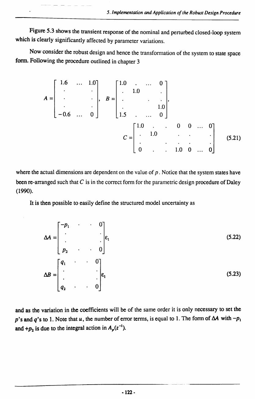
5. Implementation and Application of the Robust Design Procedure
Figure 5.3 shows the transient response of the nominal and perturbed closed-loop system
which is clearly significantly affected by parameter variations.
Now consider the robust design and hence the transformation of the system to state space
fonn. Following the procedure outlined in chapter 3
1.6 1.0 1.0 0 1.0
A= , B= 1.0
-0.6 0 1.5 0
1.0 0 0 0
c= 1.0 (5.21)
0 1.0 0 0
where the actual dimensions are dependent on the value of p. Notice that the system states have
been re-arranged such that C is in the correct form for the parametric design procedure of Daley
(1990).
It is then possible to easily define the structured model uncertainty as
-PI 0
M= £1 (5.22)
P2 0
ql 0
M= £1 (5.23)
q2 0
and as the variation in the coefficients will be of the same order it is only necessary to set the
p's and q's to 1. Note that u, the number of error terms, is equal to 1. The form of M with -PI
and +P2 is due to the integral action in A,(Z-I).
·122 -

5. Implementation and Application of the Robust Design Procedure
5.3.2 Problems Associated with the Parametric Method of Fahmy and O'Reilly
The parametric design method ofFahmy and 0' Reill y ( 1988) has consistently had problems
calculating an output feedback controller for transfonned polynomial systems. The problem
appears to be linked with the structure of the open-loop system matrices and the following outlines
how the method fails.
Considering the given example, but not transfonned such that C = [I : 0] (which is
unnecessary for this method), with p = 3 the system matrices are
0 -0.6 0 0 0 1.5 0 0 0 1 1.6 0 0 0 1 0 0 0
A= 0 0 0 0 o , B= 0 1 0 0, 0 0 0 0 0 0 0 1 0 0 0 0 0 0 0 0 0 1
0 1 0 0 0
C= 0 0 1 0 0
(5.24) 0 0 0 1 0 0 0 0 0 1
and the desired closed-loop eigenvalues are [0.75 ±jO.2 -0.01 -0.02 -0.03].
First stage - right eigenvector assignment
Choose s = 3, hence require three free parameter vectors which are chosen randomly as
0.0329 0.0329 - 0.2530 0.8892 0.8892 5.2730
Fs = ft. [2 kl = _ 10.7023 - 10.7023 - 6.1485 (5.25)
0.7486 0.7486 9.6141
The first three right eigenvectors are then calculated as
0.71- jO.31 0.71 + jO.31 1.24
-0.91 + jO.l5 -0.91 - jO.l5 -0.61
Vs = [y. Y2 ~]= 1.11- jO.30 1.11 + jO.30 -527.30 (5.26)
- 13.32 + j3 .55 -13.32 - j3 .55 614.85
0.93 - jO.25 0.93 + jO.25 -961.41
-123 •
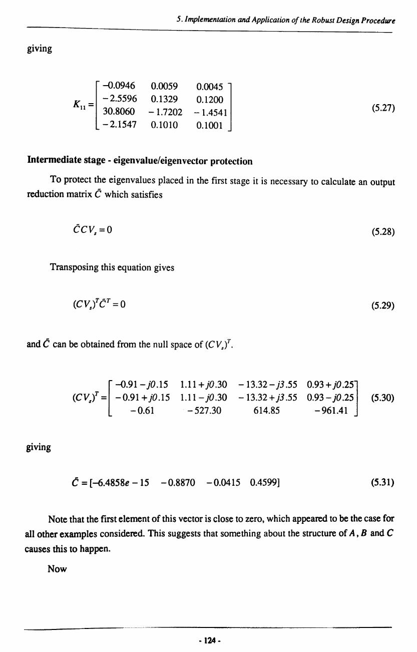
5. Implementation and Application of lhe Robust Design Procedure
. . gIvIng
~.0946 0.0059 0.0045 - 2.5596 0.1329 0.1200
Ku = 30.8060 -1.7202 -1.4541 (5.27)
- 2.1547 0.1010 0.1001
Intermediate stage - eigenvalue/eigenvector protection
To protect the eigenvalues placed in the first stage it is necessary to calculate an output
reduction matrix t which satisfies
tcvs =0
Transposing this equation gives
and t can be obtained from the null space of (CVsl.
giving
[
~.91- iO.15 (CVsl = -0.91 + iO.15
-0.61
1.11 + iO.30 1.11-i0.30
-527.30
-13.32 - i3 .55 - 13.32 + i3 .55
614.85
t = [-6.4858e -15 -0.8870 -0.0415 0.4599]
0.93 + ~O.25] 0.93 - }O.25
-961.41
(5.28)
(5.29)
(5.30)
(5.31)
Note that the first element of this vector is close to zero, which appeared to be the case for
all other examples considered. This suggests that something about the structure of A, B and C
causes this to happen.
Now
- 124-

5.lmplementalion and Application of the Robust Design Procedure
0 -0.7418 0.0088 0.0068 0 1.0 1.5054 0.0059 0.0045 0
Al =A +BKIC = 0 -2.5596 0.1329 0.1200 0 (5.32) 0 30.8060 -1.7702 -1.4546 0 0 -2.1547 0.1010 0.1001 0
CI = tc = [0 - 6.4858e - 15 - 0.8870 - 0.0415 0.4599] (5.33)
and the second stage design is based on AI' Band C l' The leading zeros in Clare a result of the
combination of the zero in t and the structure of the first two columns of C.
Second stage -left eigenvector assignment
This stage assigns the remaining two eigenvalues and their associated left eigenvectors.
The two free parameters, which are scalars, are chosen as
[ 3.4949 ]
G, = _ 12.5092
giving the eigenvectors as
W,T=~ ~]=
-D.3523e - 13 0.7041e -15
154.9955 7.2569
- 80.3684
0.2266e -13 -0.6715e -15
-369.8497 -17.3164 191.7748
The effect of the leading zeros in C1 can clearly be seen. Recall that
and the matrix W,Bl is
-125 -
(5.34)
(5.35)
(5.36)

5. Implementation and Application of the Robust Design Procedure
W)11 = [--o.5213e - 13 154.9955] 0.3332e -13 - 369.8497
(5.37)
which is certainly close to singular and is the cause of the failure of the method.
The problem does appear to be closely related to the structure of C, particularly the first
two columns. To eliminate the zeros in these columns a state transformation could be used.
Selecting
0.9103 0.3282 0.2470 0.0727 0.7665 0.7622 0.6326 0.9826 0.6316 0.4777
T= 0.2625 0.7564 0.7227 0.8847 0.2378 (5.38)
0.0475 0.9910 0.1534 0.2727 0.2749 0.7361 0.3653 0.6515 0.4364 0.3593
the transformed system is
-12.0329 -7.5397 -10.2049 -6.0669 -8.6642
-12.8911 -8.1191 -11.0231 -6.5661 -9.2630
A' = T-1AT = 11.8317 7.5256 10.2769 6.1440 8.4681 (5.39)
0.8081 0.4876 0.6447 0.3776 0.5905
15.3245 9.4643 12.6977 7.5067 11.0975
-6.2748 0.0613 0.9066 7.6603
-5.9431 0.8272 2.0939 5.7442
B'=T-1B = 4.0784 -1.7437 -0.3933 - 3.8486 (5.40)
0.7715 1.8398 -1.2741 -1.3003
10.5666 -0.0395 -1.7258 -10.1938
0.7622 0.6326 0.9826 0.6316 0.4777
0.2625 0.7564 0.7227 0.8847 0.2378 (5.41) C'=CT = 0.0475 0.9910 0.7534 0.2727 0.2749
0.7361 0.3653 0.6515 0.4364 0.3593
Performing the design using the same free parameters, it is found that Kll for the first stage
is the same as previously. Also (CV"l is the same leading to
c = [-6.4858e -15 -0.8870 -0.0415 0.4599] (5.42)
-126 -

5. Implementation and Application o/the Robust Design Procedure
as before and
C1 = [0.1038 -0.5441 -0.3726 -0.5953 -0.0571]
In the second stage
-18.1343 43.279 95.0704 -226.8566
WT = , 65.1146 -155.3763 104.0310 -248.2383 9.9754 -23.8032
which appears to have removed the problem of leading zeros. However
W,B = [ 0.1335e - 11 1 -0.3024e -11
154.9955 ] -369.8497
and again the problem of singularity stops a solution being obtained.
(5.43)
(5.44)
(5.45)
The fact that the problem is related to the structure of C can be verified by changing some
of its elements. It was found that only two elements needed to be changed in order for a solution
to be obtained, and as would be expected these are in the first two columns. For example with
o 1 0 0 0
C = 0.219 0.047 1 0 0 o 0 0 1 0 o 0 0 0 1
a solution is obtained where
-10.4063 30.9594 2.4719 -2.6056
K, = 31.4037 0.1382 0.1248 -1.7946 -1.5172
-2.1898 0.1054 0.1038
-127 -
-15.3845 0.0002
o o
(5.46)
(5.47)

5. Implemenuuion and Application of the Robust Design Procedure
It should be pointed out that a number of differen t strate gies for overcoming the encountered
problems were tried. These included specifying different desired closed-loop eigenvalues,
assigning the left eigenvectors first and changing the split between the two stages. However no
approach managed to ensure that a solution could be obtained. Another possibility is to use a
different canonical form in the transformation from polynomial to state space representations.
This however does not alleviate the problem as a similar structure for the C matrix is obtained
when the dynamic compensator is augmented with the system.
The most probable reason for the failure of the method is overprotection. To explain,
consider the equation
(5.48)
where V, represents the matrix of the first s right eigenvectors assigned in the first stage. Recall
from chapter three that t must be chosen such that this equation is satisfied for the first s right
eigenvectors to be protected from subsequent feedback loops. This equation can also be inter
preted as requiring Vs to lie in the null space of t C . If the dimension of this null space is greater
than s then other right eigenvectors may be protected leading to overprotection and the method
would fail in the second stage, as is the case here.
A complete analysis of this problem and an investigation into ways of overcoming it is
really outside the scope of this work, hence the parametric method of Daley (1990) will be used
as the basis of the state space design.
5.3.3 Determining the Number of Free Parameters
Chapter four outlined how to avoid subjecting the optimisation procedure to constraints
by effectively re-defining the free parameters as the scalar multipliers of the basis vectors of
various null spaces. Hence to determine the number of free parameters it is necessary to obtain
the dimensions of the null spaces involved and this section outlines how this is achieved.
Consider the system as outlined in section 5.3.1. There will be p + 2 states, p + 1 inputs
and p + 1 outputs, hence
n =p+2
r=p+l
m =p+l
-128 -
(5.49)
(5.50)
(5.51)

so
and
5. Implementation and Applicalion O/lhe Robust Design Procedure
Clearly
q=n-r=p+2-p-1=1
FI = [[I ... [,]
F2 = fL]
Recall that the whole of F} is selected from the null space of~, where
~=
(5.52)
(5.53)
(5.54)
(5.55)
(3.56)
In this case the ex's are all chosen as 1 and the dimension of ~ is clearly (r x rm) as q = 1
and the dimension of Mile is (r x m ).
Section 5.2 discussed details of the implementation which included a section on how to
calculate the null space of a matrix using its singular value decomposition. From this the
dimension of the null space of ~ can be deduced as (rm x (rm - r », assuming full rank. Thus the
number of free parameters used in the calculation of F} is rem -1).
The remaining vectors in F2 are each obtained by calculating the null space of Zit
(i = r + 1 --+ n). In this case there is only one F2 vector and it lies in the null space of
(5.57)
-129 -

5. Implementalion and Application of the Robust Design Procedure
The dimension of Z" is obviously (r x r), so the existence of the null space is dependent
on the rank of the matrix. Daley (1990) has shown that this null space will exist and that the rank
of Z" will be deficient by at least 1. Hence the dimension of the null space will be (r x 1) and
only one free parameter is needed for the calculation of the F2 vector.
This brings the total number of free parameters, Nf to
Nf = r(m - 1) + 1 (5.58)
5.3.4 Selecting the Optimisation Routine
This section considers the choice of the optimisation algorithm. For simplicity and to allow
a quick assessment of the robust design approach it was decided to use algorithms that require
no derivative information. It is recognised that derivative information will generally improve
the efficiency of optimisation in all areas, and algorithms that utilise such information could be
used if unsatisfactory results are obtained from the function value only algorithms.
Most routines of this type in the NAG library are based on the quasi-Newton method,
which really only leaves the question of whether the problem is of a least squares type. The only
cost function which easily fits this description is the eigenvalue differential cost function, J1•
Note that for this example u = 1 so there are only n residual terms in the function. For any real
benefit to be gained by describing the problem in a least squares manner, the number of residuals,
N" should be greater than the number of variables (or free parameters), Nf , i.e.
or r(m - 1) + 1 > n (5.59)
For p = 1, N, = 3 and N" = 3 and as p increases Nf increases at a higher rate than N". Thus
there is no justification in expressing the problem in a least squares framework, hence it was
decided to use NAG routine E04JAF to perform the optimisation. Further details of this routine
can be found in appendix C.
5.3.5 Layout of the Results
All the results will be laid out in the following format
x) Initial comments
- 130-

WT = [ ... J
J . = ... or.g
5. Implementation and Application of the Robust Design Procedure
lopl y = ...
EigenvaluelEigenvector Sensitivities:
0.75±jO.2 -0.01 -0.02 ...
orig ... . .. . ..
opt ... . .. . ..
orig ... . .. . ..
opt ... . .. . ..
Pole Positions:
Original Perturbed Distance Moved
Controller Polynomials:
F/z- I) = .. .
G/z-I )= .. .
H/z-I) = .. .
Final comments
Where
x specifies a reference number for the particular set of results. Hence when discussing
results only this number need be quoted.
Initial comments
These comments briefly introduce the set of results explaining what they represent.
XT is a vector that specifies the initial values for the free parameters, where the first r(m - 1)
elements are used in the calculation of FI , and the remaining element in the calculation
of F2•
WT is a vector that specifies the value of the weights used. Clearly the interpretation is
dependent on the cost function being used.
--_. ----_ .. _._ ..• _-
- I ~ I -
5. Implementation and Application o/the Robust Design Procedure
- specifies the n eigenvalue sensitivity weights ~i
- for the eigensttucture differential cost function, specifies the
weights 1li' and for the transient response differential cost
function specifies the weights "Ii
- specifies the weight cr
For the conditioning cost function no weights need to be specified.
lori, specifies the value of the cost function at the starting point.
lop, y specifies the value of the cost function at the final point. The value ofy is used to indicate
the conditions under which the routine terminated.
y = 1 - indicates that a minimum point was found.
y = 2 - indicates that not all the conditions for a minimum were satisfied but
that no lower point could be found.
EigenvaluelEigenvector Sensitivities:
The eigenvalue sensitivities are given in the first two rows followed by the eigenvector
sensitivities. For each entry there are two numbers. The upper entry corresponds to the
sensitivity at the starting point and the lower one to the sensitivity at the final point. For
the eigenvalue differential cost function results there will clearly not be entries for the
eigenvector sensitivities and for the conditioning cost function results this table will not
be given.
Pole Positions:
The first column of this table corresponds to the closed-loop pole positions for the
nominal system, the second column to the closed-loop pole positions for the perturbed
system and the third to how far the poles have actually moved. This table is only given
for relatively good results and always for the conditioning cost function results.
Controller Polynomials:
The three controller polynomials are only specified for particularly good sets of results.
Final comments
These contain any conclusions that can be drawn and outline the reasons behind the
decisions for the next set of results, e.g. how the weights should be changed.
·132·

5.lmpiementalion and Application of the Robust Design Procedure
5.3.6 Results for the Eigenvalue Differential Cost Function
The following results were obtained for the system described in (5.16), using the eigenvalue
differential cost function. The desired closed-loop pole positions are 0.75 + jO.2 and the maxi
mum level of perturbation was assumed to be +50% of the nominal values of the A/z-1) and
Bp(Z-l) polynomial coefficients. The value of p represents the order of the controller.
p=1
1) The starting point is randomly selected and as no infonnation is available on suitable
weights they are all set to 1.
XT = [0.3586 0.8694 - 0.2330]
WT = [1.0 1.0 1.0]
Jorig = 1.792632
Eigenvalue Sensitivities:
0.75±jO.2 -0.01
orig 0.9463 0.4071e-l
opt 0.9463 0.4071e-l
Joptl = 1.792632
No improvement in the sensitivities so try a different starting point.
2) Again the starting point is randomly selected and the weights are all set to 1.
XT = [3.8833 66.1931 - 93.0856]
WT = [1.0 1.0 1.0]
Jon, = 1.792632
Eigenvalue Sensitivities:
0.75±jO.2 -0.01
orig 0.9463 0.4071e-l
opt 0.9463 0.4071e-l
J opt 1 = 1.792632
Again no improvement at all and note that the sensitivities are the same as in 1). A number
of other starting points were tried with the same result and the weights were also changed
but did not effect the outcome. It appears that with p = 1 no significant improvement in
robustness can be achieved, so try increasing p.
·133 -

5. Implementation and Applicalion oflhe Robusl Design Procedure
p=2
3) As with the previous results the starting point is randomly chosen and the weights all set to 1.
XT = [~.0101 ~.0392 0.0012 0.0011 -0.0226 -0.0129 -0.0351]
WT = [1.0 1.0 1.0 1.0]
Jorig = 8.021354 JOpt2 = 1.789106
Eigenvalue Sensitivities:
0.75±jO.2 -0.01 -0.02
orig 0.9824 1.7910 1.6980 opt 0.9452 0.6246e-l 0.4555e-l
Clearly with the p = 2 case there is scope for improvement, however it is necessary to
adjust the weights to concentrate more on the dominant eigenvalue sensitivities. A different
starting point is also used to see if a lower initial function value can be obtained.
4) The starting point is again randomly selected and the weights adjusted to place more
emphasis on the dominant eigenvalues.
XT = [0.0022 ~.0242 -0.0356 -0.0037 -0.0170 0.0089 0.0027]
WT = [1.0 1.0 0.1 0.1]
Jorig = 1.783400 Jopt2 = 1.782130
Eigenvalue Sensitivities:
0.75±jO.2 -0.01 -0.02
orig 0.9437 0.8S48e-l 0.l224
opt 0.9428 0.1304 0.1660
Note that the initial function value is lower than the final function value of3). Other starting
points were tried but no lower initial value was obtained, hence the values used here
represent a good starting point. Examining the sensitivities it is again clear that the weights
need to be adjusted to concentrate even more on the dominant eigenvalue sensitivities.
S) Using the same starting point as 4), the weights were continually adjusted through a number
of iterations leading to the result presented here.
- 134-

5. Implementation and Application of the Robust Design Procedure
XT = [0.0022 -0.0242 -0.0356 -0.0037 -0.0170 0.0089 0.0027]
WT = [1.0 1.0 0.0001 0.0001]
lorig = 1.781173 lOP/2 = 0.527665
Eigenvalue Sensitivities:
0.75±jO.2 -0.01 -0.02
orig 0.9437 0.8548e-1 0.1224
opt 0.4023 32.39 31.47
A significant improvement in the dominant eigenvalue sensitivities has been achieved but
at the expense of the sensitivities of the other poles. At this stage it is useful to detennine
the pole positions for the perturbed closed-loop system to assess how good this result is.
Pole Positions:
Original Perturbed Distance Moved
0.75±jO.2 0.6981 ± jO.3395 -D.0519 ± jO.1395
-0.01 0.2315 0.2415
-0.02 0.0013 0.0213
One of the controller poles has become quite significant and so this solution is not
particularly good even though the dominant pole movement has been very much reduced.
By adjusting the weights it should be possible to overcome this problem.
6) For the same starting point as 4), the results presented here are the best compromise that
could be achieved between reducing the dominant eigenvalue sensitivity and increasing
the sensitivities of the other poles.
XT = [0.0022 -0.0242 -0.0356 -0.0037 -0.0170 0.0089 0.0027]
WT = [1.0 1.0 0.0005 0.0005 J
lorig = 1. 78 1 18 1 i opI2 = 1.023105
Eigenvalue Sensitivities:
0.75±jO.2 -0.01 -0.02
orig 0.9437 0.8548e-l 0.1224
opt 0.5692 19.64 19.10
Pole Positions:
- 135 -

5. Implementation and Application of the Robust Design Procedure
Original Perturbed
0.75±jO.2 0.7869 ± jO.3611 -0.0099
-0.0201
Controller Polynomials:
Fp(Z-I) = 1.0-0.0640z-1-O.2027z-2
Gp (Z-I) = 0.1940 -0.2329z-1 +0.0812z-2
Hp (Z-I) = 0.0704 - 0.0282z-1
0.0967
0.0025
Distance Moved
0.0369±jO.1611
0.1066
0.0226
The transient response of the closed-loop system with this controller is shown in figure
5.4 which is clearly a significant improvement over the response for the minimum order
controller shown in figure 5.3. Of course it is natural to consider what level of improvement
can be achieved by increasing p further.
p=3
7) Repeating the same procedure as above a good starting point was found and the weights
adjusted to achieve a satisfactory compromise but with a significant level of improvement.
XT = [-0.0724 -0.6805 -1.8138 -2.9852 -4.5878 -2.7362 -1.7356
-3.1889 0.8057 3.4629 0.8311 -1.8653 -0.8210]
WT = [1.0 1.0 0.0 0.0005 0.0005]
Jorig = 1.583238 J Opl 1 = 1. 163915
Eigenvalue Sensitivities:
0.75 ±jO.2 -0.01 -0.02 -0.03
orig 0.8877 0.3603e-1 2.6900 2.6830
opt 0.6385 2.298 19.98 17.26
Pole Positions:
Original Perturbed Distance Moved
0.75 ±jO.2 0.8094 ± jO.3646 0.0594 ± jO.1646
-0.0098 -0.0079 0.0019
-0.0201 0.0222 ±jO.0193 0.0423 ± jO.0193
-0.0301 0.0523 :!: )0.0193
- 136-

5. Implementation and Application of the Robust Design Procedure
This is quite a good result but comparing it with 6), the best result for the p = 2 case, it
can be seen that the dominant pole sensitivities are not as good here. However it was
expected that with p = 3 a better result would be obtained. Try a different starting point.
8) A number of alternative starting points were tried and the procedure for adjusting the
weights carried out in each case. The best result obtained is presented here.
XT = [0.5634 -0.2503 1.0725 -1.8525 -1.8031 -3.0674 2.3256
-1.4839 -0.9125 -4.3826 -6.6312 -0.6958 -6.5606]
WT = [1.0 1.0 0.002 0.0001 0.002]
JO';I = 1.798684 lOPll = 1.017731
Eigenvalue Sensitivities:
0.75±jO.2 -0.01 -0.02
orig 0.9483 0.1555 0.4801
opt 0.5661 9.5444 0.8613
Pole Positions:
Original Perturbed
0.75±jO.2 0.7861 ±jO.3603
-0.01 -0.0195
-0.02 0.0044
-0.03 0.0846
Controller Polynomials:
Fp(Z-I) = 1.0 - 0.0366z-1 - 0.2071z-2
- 0.0040z-3
Gp(Z-l) = 0.1966 -0.2326z-1 +0.0779z-2 +0.OOI6z-3
Hp(Z-I) = 0.0725 - 0.0290z-1
-0.03
0.2811
9.8610
Distance Moved
0.0361 ±jO.1603
-0.0095
0.0244
0.1146
Note that a better result was obtained from what would be classed as a worse starting point
as the initial function value is higher than for 7). This illustrates the fact that these functions
probably have many local minima and it is extremely important to try a number of alter
native starting points. The transient response for the closed-loop system with this controller
is shown in figure 5.5. Clearly this result is only a slight improvement over the p = 2 case
which suggests that this type of result represents the best level of improvement that can
be obtained. To verify consider increasing p again.
·137·

5.lmpiementation and Application of the Robust Design Procedure
p=4
9) After trying a number of randomly chosen starting points and suitable adjustment of the
weights, this result was the best obtained.
XT = [-1.3462 -3.7481 -3.6908 -{).6515 -1.0806 -3.9009 -3.4066
3.4978 -3.1640 -1.5535 -1.6996 -{).0319 0.2454 -1.4202
-1.6027 0.3568 -1.4492 -{).0576 -2.1061 -{).7171 -1.1195]
WT = [1.0 1.0 0.003 0.002 0.002 0.003]
lori, = 2.694211 IOPI 1 = 0.808537
Eigenvalue Sensitivities:
0.75±jO.2 -0.01 -0.02 -0.03 -0.04
orig 1.1430 0.9609 2.7600 1.1640 4.5700
opt 0.4816 7.0310 3.8370 3.1740 6.9960
Pole Positions:
Original Perturbed Distance Moved
0.75±jO.2 0.7530±jO.3517 0.OO30±jO.1517
-0.0099 0.1210
-0.0199 -0.0173
-0.03 -0.0322
-0.0401 0.0046
Controller Polynomials:
Fp{Z-l) = 1.0 - 0.0359z-1 - 0.2681z-2
- 0.0131z-3 - 0.1481e - 3z-4
Gp{Z-I) = 0.2359 - 0.2870z-1 + 0.0913z-2 + 0.0051z-3 + 0.5933e - 4z-4
H,(Z-l) = 0.0754 - 0.0302
0.1309
0.0026
-0.0022
0.0447
On initial inspection this appears to be significantly better than both the p = 2 and the p = 3
cases. However one of the controller poles has moved considerably but even at 0.1210 it
could be argued that it would still not significantly influence the shape of the response.
The transient response associated with this controller is shown in figure 5.6 and clearly it
is better than has been obtained previously, but only just. It certainly suggests that the
benefits of considering controllers beyond third or fourth order is questionable.
- 138-

5.lmplementalion and Application of the Robust Design Procedure
5.3.7 Results for the Eigenstructure Differential Cost Function
This cost function contains the eigenvector differential and to help determine if this term
leads to better solutions, the same starting points for the best results for the eigenvalue differential
cost function are used. Also from the previous set of results it is clear that the case of p = 1 need
not be considered.
p=2
10) Using the same starting point as 6) and refining the weights lead to two sets of results
presented here and in 11).
XT = [0.0022 -0.0242 -0.0356 -0.0037 -0.0170 0.0089 0.0027]
WT = [1.0 1.0 5.0e - 4 5.0e - 4 1.0 1.0 1.0 1.0e - 2 1.0e - 4]
lori, = 1.921558 10Pl2 = 1.789696
EigenvaluelEigenvector Sensitivities:
0.75±jO.2 -0.01 -0.02
orig 0.9437 0.8548e-1 0.1224 opt 0.9455 0.270ge-3 0.3976e-1
orig 2.6830e2 4.1390e2 4.5320e4
opt 7.7010 2.1200 1.751Oe2
11) Second result
XT = [0.0022 -0.0242 -0.0356 -0.0037 -0.0170 0.0089 0.0027]
WT = [1.0 1.0 5.Oe - 4 5.0e - 4 1.0 1.0 1.0 I.Oe - 2 1.0e - 6]
lori, = 1.782585 10pI2 = 1.317259
EigenvaluelEigenvector Sensitivities:
0.75±jO.2 -0.01 -0.02
ong 0.9437 0.8548e-1 0.1224
opt 0.7054 12.07 11.75
orig 2.6830e2 4.1390e2 4.5320e4
opt 2.542004 1.2840e5 9.4000e4
·139 -

5./mplemenuuion and Application of the Robust Design Procedure
Examining the results in 10) and 11) it can be seen that there appears to be a conflict
between the dominant eigenvalue sensitivities and their associated eigenvector sensiti
vities. When the dominant eigenvalue sensitivities are decreased the eigenvector sensiti
vities increase and vice versa. A number of alternative starting points were tried but all
were subject to this conflict and no satisfactory result could be obtained.
A value of p = 3 was used with the same starting point as 8) to determine if this problem
could be overcome by introducing more design freedom. However the conflict was still
present and it is felt that increasing p further would not help in this situation.
Perhaps a better approach to the application of this cost function would be to start at the
sub-optimal points found using the eigenvalue differential cost function. The aim would
then be to try and reduce the eigenvector sensitivities without adversely affecting the
eigenvalue sensitivities.
12) Using the sub-optimal point found in 6) as the starting point and again refining the weights
as before.
p=3
XT = [0.0086 -{).0173 -0.0420 0.0032 -0.0234 0.0063 -0.0018]
WT = [1.0 1.0 5.0e - 4 5.0e - 4 1.0 1.0 1.0e - 4 1.0e -7 5.Oe - 10]
lori, = 1.116970 lopt 2 = 1.098190
EigenvaluelEigenvector Sensitivities:
0.75±jO.2 -0.01 -0.02
orig 0.5692 19.64 19.10
opt 0.6052 17.55 17.06
orig 9.3860e7 1.4490e8 1.0570e10
opt 6.6140e7 1.0200e8 7.4690e9
This result is quite encouraging as some improvement has been made. However by
examining the transient response of the closed-loop system with the controller for this
result, figure 5.7, it can be seen that the level of improvement in the eigenvector sensitivities
really needs to be much greater to have any significant effect on performance robustness.
A higher value of p could achieve this.
------------------------------- 140-

5.lmplemenlation and Application of the Robust Design Procedure
13) This time the sub-optimal point found in 8) is used as the starting point and appropriate
weights selected.
XT = [133.8 -25.6 395.1 -365.1 12.1 -1214.0 173.6
-254.0 -23.5 -622.4 -1672.8 -205.3 -929"+]
WT = [1.2 1.2 2.0e - 3 1.0e - 4 2.0e - 3 1.0 1.0
l.Oe - 6 l.Oe - 6 1.0e - 6 1.0e - 4]
Jorig = 1.639185 JopI2 = 1.320894
EigenvaluelEigenvector Sensitivities:
0.75 ±jO.2 -0.01 -0.02 -0.03
orig 0.5661 9.5440 0.8613 9.8610
opt 0.5726 9.4594 0.6515 9.5769
orig 2.4360e3 4.5300e7 5.1630c6 1.0150e7
opt 8.3265e2 3.3762e7 3. 1700c6 1.4671e7
This is a slightly better improvement than in 12) but by comparing the transient response
shown in figure 5.8 with that in figure 5.5 (the result from the eigenvalue differential cost
function), it can be seen that no real improvement has been achieved. Assuming this is the
typical improvement that can be expected when p is increased, it would suggest that a very
high order controller is needed to gain any real advantage over the controllers obtained
using the eigenvalue differential cost function.
5.3.8 Results for the Transient Response Differential Cost Function
From the modal decomposition it was seen that for performance robustness a slightly
different form for the eigenvector differential was more appropriate and was included in the
transient response differential cost function. From the previous results it would seem reasonable
to start from the sub-optimal points found using the eigenvalue differential cost function and
only the case of p = 3 is considered.
14) Using the sub-optimal point found in 8) and after refinement of the weights the following
result was obtained.
XT = [133.8 -25.6 395.1 -365.1 12.1 -1214.0 173.6
-254.0 -23.5 -622..+ -1672.8 -205.3 -929.4]
- 141 -

5. Implementation and Application of the Robust Design Procedure
WT = [1.0 1.0 2.0e - 3 1.0e - 4 2.Oe - 3 1.0 1.0
1.0e - 4 1.0e - 4 1.0e - 4 1.Oe -7]
lorig = 1.639185 lOPI2 = 1.320894
EigenvaluelEigenvector Sensitivities:
0.75±jO.2 -0.01 -0.02 -0.03
orig 0.5661 9.5440 0.8613 9.8610 opt 0.5722 9.6320 0.3183 9.4160
orig 1.5640e6 4.7530e7 1.2000e8 1.1l90e8 opt 8.9320e4 1.5950e7 3.0490e7 1.5060e7
This is very similar to the result in 13) and by examining the transient response in figure
5.9 it can be seen that no real improvement over that shown in figure 5.5 has been achieved.
Again it is expected that a very high order controller would be required to make any
significant improvement in the eigenvector sensitivities.
5.3.9 Results for the Conditioning Cost Function
This cost function is quite different to the others as it is not directly concerned with
sensitivities. No weights are needed so the problem of iteratively refining them does not exist.
On the basis of the previous results it was decided to restrict the investigation to the cases of
p = 2 and p = 3.
p=2
15) A number of randomly selected starting points were tried and this was the best result
obtained.
X T =[-D.0243 -0.0113 -D.0083 -0.1591 -0.0685 -0.25180.0159]
lorig = 58.251362 i opl2 = 14.445608
Pole Positions:
Original Perturbed Distance Moved
0.75 ±jO.2 0.8854 ±jO.3750 0.1354 ±jO.1750
-0.01 -0.0098 0.0002
-0.02 -0.0200 0.0000
- 1-l2 -

p=3
5. Implementation and Application of the Robust Design Procedure
This is clearly not as good as the result obtained using the eigenvalue differential cost
function for the p = 2 case, which can be verified by comparing the transient response in
figure 5.10 with that in figure 5.4. Indeed the response is only slightly better than that for
the minimum order controller shown in figure 5.3. A higher value of p may yield a more desirable result.
16) Again a number of randomly selected starting points were tried and this represents the best
result obtained.
XT = [-0.5621 -0.9059 0.3577 0.3586 0.8694 -0.2330 0.0388
0.6619 -0.9309 -0.8931 0.0594 0.3423 -0.9846]
lOTig = 1.847105e3 JOPl2 = 25.646076
Pole Positions:
Original Perturbed Distance Moved
0.75±jO.2 0.8872±jO.3751 0.1372±jO.1751
-0.01 -0.0082 0.0018
-0.02 -0.0239 -0.0039
-0.03 -0.0300 0.0000
This result is very similar to that in 15) and again the transient response shown in figure
5.11 is significantly worse than that in figure 5.5 (the best result from the eigenvalue
differential cost function).
5.4 Summary and Discussion of the Results
This chapter has considered the application of the proposed robust design method to a
simple polynomial system to help illustrate the design procedure and give an indication of the
improvement that can be achieved.
With the application of the method a number of issues regarding its implementation arise.
These aspects are important as they can have a significant effect on the performance of the design
procedure. From the results it is clear that it is necessary to perform the optimisation, which
involves carrying out the state space design, many times to help in the selection of appropriate
weights. Because of this, it is desirable to implement the method such that the optimisation can
be performed reasonably quickly without sacrificing accuracy. For these reasons a joint Pro
Matlab / Fortran 77 implementation is adopted.
·143·

5./mpiementalion and Application of the Robust Design Procedure
The frrst step of the design is to transfonn the system to state space fonn which then allows
the model uncertainty to be defined. In this case the uncertain parameters are of the same
magnitude and vary by the same amount leading to a simple definition of the uncertainty.
The problems with the parametric method of Fahmy and O'Reilly (1988) were then dis
cussed in depth for this example and it was concluded that the method of Daley (1990) should
be used for the state space design. It was then possible to show how to detennine the number of
free parameters in the design and hence decide on an appropriate optimisation routine.
The results for each cost function were then presented for values of p (the order of the
controller) in the range of 1 to 4. Note that the lowest value of p must be chosen such that
r +m > n, which is a requirement of the parametric state space design, and that it may not
necessarily always be 1.
There are a few interesting points to note about the results. Firstly, the refinement of the
weights is relatively easy with typically up to 4-5 iterations needed to find a good solution. Their
choice is quite straightforward if based on the associated sensitivities and if a model of the
perturbed system is available such that the perturbed closed-loop pole positions can be examined.
Secondly, the cost functions which utilise eigenvector differential infonnation, do not
appear to produce results which are significantly better than those obtained using the eigenvalue
differential cost function. Of course it is expected that the eigenvalue sensitivities will be the
most important as they affect the rate of rise and decay of the transient response. However the
eigenvector sensitivity information should have helped produce better solutions. Examining the
results shows that a conflict between the eigenvalue and eigenvector sensitivities appears to
arise. This conflict prevents good solutions from being obtained. The most probable reason for
this is that the method does not have the freedom necessary to reduce all the sensitivities. This
was verified by the results which showed that for higher values of p, where there is greater design
freedom, there was a slightly better improvement. The problem, however, is that to yield sig
nificantly better results it is expected that a very high order controller would be required.
Lastly considering the transient responses of the various controllers it is clear that a sig
nificant improvement can be achieved using the eigenvalue differential cost function but the
conditioning cost function only produced a slight improvement over the minimum order
controller. This is almost certainly due to the fact that conditioning is quite a general criteria
which, among other factors, minimises an upper bound on the sensitivities of 1lll the eigenvalues.
The results for the eigenvalue differential cost function with all the eigenvalues weighted evenly
showed that very little improvement in their sensitivities could be achieved, which explains what
is effectively happening with the conditioning cost function.
-144 -

5. Implementation and Application of the Robust Design Procedure
This highlights the fact that it is often necessary to sacrifice the sensitivity of certain poles
such that the sensitivity of other poles can be improved. In this case the controller or added poles
are placed close to zero and as such have little effect on the transient response compared with
the two dominant poles. The sensitivity of the dominant poles can then be decreased by allowing
the sensitivities of the added poles to become large, which is verified by examining the results.
This trade off is quite important as it requires the choice of the weights to be made with some
care so as not to allow the added poles to have a significant effect on the transient response when
the system is subject to model uncertain ty. It is reall y necessary to have some idea of the maximum
level of parameter variations in order that the movement of the added poles subject to this
maximum change can be checked to ensure that they do not become dominant. In this case the
aim was to keep the added poles within the z = 0.1 circle for the maximum variation of 50%.
Figure 5.6 illustrates the best transient response behaviour when the system is subject to
parameter variations. As the order of the controller, p is increased there are more free parameters
in the design process, so it is expected that higher order controllers would yield better results
which is verified here as the corresponding controller for figure 5.6 is fourth order.
-14S -

5./mplementalion and Application of the Robust Design Procedure
P is the order of the controller
To obtain the correct fonn for C
Adjust
Free Parameters
Specify Polynomial System
Transfonn to State Space Fonn
State Transfonnation
Select Initial Free Parameters
Perfonn Parametric Design
Evaluate Cost Function
N
Generate F and G from K
Figure 5.1 - Flowchart of the Robust Polynomial Controller Design Procedure
Note: F ,a and H are controller polynomials in terms of the backward shift operator, Z-I.
K is the state space output feedback malrix.
The paramelric design stage is expanded in figure 5.2.
-146 -

Note:
5. Implementation and Applicalion of lhe Robusl Design Procedure
Calculare the Null Space of c:
Calculate r From this Null Space
Calculate vi
i=ltor
i = r+l y r----~ i>n
i = i+l
Calculate the Null Space ofZi
Calculate ~
From this Null Space
Calculate vi
i=r+lton
Calculate W = Inverse of V
Figure 5.2 - Flowchart of the Parametric State Space Design Procedure
c=
V=£L ... ~]
!; = (~/-ArIBJj ~ =1-FIVl:£('A,/-ArlB]r
t r= L
Vu = the 1st r rows of the 1st r right eigenvectors.
F, = [[I" ·Ll andF2 = [£+1" '["1
-147 -

J
J
I
5. Implementation and Application of the Robust Design Procedure
2
1.5 -1 f-
0.5 f-
0 --0.5 -
-1
-1.5 I-
-2 0
2
1.5
1
0.5
0
-0.5
-1
-1.5
-20
! 1\
t A
A I
-r I
- i 11 r i . - 1-'-1 r-· !
V i . I i · i i 1 · I I I · i I 1 i I 1 1 1 1 I 1 1
i ~ ! 1\ I 1 1 1 1 1 1 i !
~if i 1
! 1 1 I 1
V 1 1
i I I i
I 1 I ! ! ! l~_ I l L i ..... i -- -
i ! i i
i v v so 100 150 200 250 300 350 400 450
Sample N"umbcr
Figure 5.3 - Response of the Closed-Loop System with the Controller derived from the
Diophantine Equation
so 100
r -i
I I 1
I I I I 1
150
· · i 1 I
I I 1 l ___ +-~
200 250
Sample N"umber
-
Figure 5.4 - Response of the Closed-Loop System with the p=2 Controller from Cost Function 1
2
1.5
1
0.5
0
-0.5
-1
-1.5
-20 50
1
I 1 I I
I 1
I L\-,.._--.....
100 150 200 250
SlU'nple N"l.,unber
Figure S.S - Response of Closed-Loop System with the p=3 Controller from Cost Function 1
------- Input __ Output
-148 -
ft
V --
--
500

I
I
I
5. Implementation and Application of the Robust Design Proceduu
2-
1.5
1
0.5
0
-0.5
-1
-1.5
-2-0 50
I
I I I I
I i I :-
100 150
, ,
I i
I t. _._ ........ ---6
200 250 300 350 400 450
Figure 5.6 - Response of Closed-Loop System with the p=4 Controller from Cost Function 1
2-
1.5
1
0.5
0
-0.5
-1
-1.5
-2-0 50 100
,- -"'-----.,. ! j
I I I I
I I !
150
, ,
i I I I I
i l _._----6
200 250
Samplo N"urnbor
Figure 5.7 - Response of Closed-Loop System with the p=2 Controller from Cost Function 2
2
1.5
1
0.5 I I I
0
-0.5 I -1
I_,~ ___ '"
-1.5
-20 50 100 150
, ,
i I I I
I
l __ ._4---1
200 250
Sample N"urnbor
400 450
Figure 5.8 - Response of Closed-Loop System with the p=3 Controller from Cost Function 2
------- Input __ Output
-149 -
500
500

I
I
J
5 . Implementation and Application of the Robust Design Procedure
2.
1.5
1
0.5
0
-0.5
-1
-1.5
-2. 0 50 100 150 200 2.50 400 450
Sarnp1e N"u~ber
Figure 5.9 - Response of Closed-Loop System with the p=3 Controller from Cost Function 3
2.
1.5 ~
1 t-
0.5 I-
0 ~
-0.5 l-
-1
-1.5 I-
-2. o
r1-' -r-I ! I
~ I I I
! I I I
! I i ! I I I :-
50 100 150
i
f ~ ! ! i
-~1 A i
r - . i I ,
I , I I I
i
~ I
I I I I I
I I " I I I I
I I
-v ; I I
; ! ! , i i i i - - 'I-
V ~ 2.00 2.50 300 350 400 450
Sa~p1e N"u~ber
Figure 5.10 - Response of Closed-Loop System with the p=2 Controller from Cost Function 4
2.
1.5
1
0.5
0
I
I -0.5 I
-1 I_~,. __ ~
-1.5
-2 0 100 50 150 200 250 300 400
Sample N"umbor
~ -
Figure 5.11 - Response of Closed-Loop System with the p=3 Controller from Cost Function 4
------- Input _Output
-ISO-
500
V --
--
500
500

5.lmplementalion and Application o/the Robust Design Procedure
REFERENCES
Daley, S. (1990)
'00 Eigenstructure Assignability using parametric output feedback'
Brunei University Control Engineering Centre Internal Report, August 1990
Edgar, S.L. (1989)
, Advanced Problem Solving with FORTRAN 77'
Science Research Associates, Henley-on-Thames, England
Fahmy, M.M. and O'Reilly, J. (1988)
'Multistage Parametric Eigenstructure Assignment by Output Feedback Control'
International Journal o/Control, v48, nl, pp 97-116
NAG (1990)
'Fortran Library Manual Mk 14'
Numerical Algorithms Group Ltd, Oxford, U.K.
PRO-MATLAB (1990)
'PRO-MATLAB User Guide'
Mathworks Inc, South Natick, Mass, U.S.A.
Wellstead, P.E. and Sanoff, S.P. (1981)
'Extended Self-Tuning Algorithm'
International Journal o/Control, v34, n3, pp 433-455
- lSI -

CHAPTER 6
APPLICATION TO A HYDRAULIC RIG
6.1 Introduction
Hydraulic systems include some of the most powerful and fast-moving devices in engin
eering and are widely used in many industrial plants. The design of controllers for such systems
can be quite difficult due to a number of factors including non-linearities (such as the relation
between flowrate and pressure), variations in oil viscosity resulting from changing temperature
and load dependent gain (Daley, 1990). Applying the proposed robust design procedure to a
realistic industrial system of this type would provide useful infomlation on the general applic
ability of the method. The hydraulic test rig considered in Daley (1987) would be a good system
to consider as it was designed and built to be representative of real industrial plants.
The rig consists of a stiff shaft which is driven by a hydraulic motor and loaded with a
hydraulic pump. The oil flow to the motor is controlled by an electrohydraulic servo-valve and
the pressure differential across the pump can be changed to increase or decrease the loading on
the shaft. A schematic of the hydraulic circuit of the rig is shown in figure 6.1.
Daley (1987) considered the application of self-tuning control to this system and assessed
the performance of the closed-loop system when subjected to varying supply pressure and load.
The results were compared to a more traditional proportional plus integral plus derivative (PID)
controller and shown to be significantly better.
The aim here is to design a fixed term controller for the system which is robust to varying
supply pressure and load, such that the performance is better than the PIO controller and hopefully
comparable to that of the self-tuning controller. Of course the self-tuning controller will in general
be more flexible to variations in the plant parameters and perform well over a wide range of
possible parameter values. However over a specified range, for which the robust fixed term
controller is designed, it is hoped that the relative performance of the two controllers will be
similar. Also, in this range the fixed term controller may even perform slightly better as there
will be no tuning transients as with the self-tuning controller.
As it is not possible to perform tests on the real rig, it is necessary to constnIct an accurate
simulation of the system. To do this, use can be made of commercially available simulation
languages which contain the basic integration algorithms necessary to perform a continuous time
-------------~-----------_._ .. _-_. __ .... - - -- .. -- -
- 152-

6. Application to a Hydraulic Rig
simulation, as well as an environment in which quite complex system equations can be specified.
In this case the Advanced Continuous Simulation Language (ACSL) package is used and further
details on the simulation can be found in the following section.
Using the simulation it is possible to show how the proposed method can be applied to a
real plant, from system identification to controller design and implementation. Three robust fixed
term controllers are developed, the first considering only variations in the supply pressure, the
second only variations in the load and the third variations in both.
6.2 Nonlinear Simulation and Model Identification
A model of the rig can be developed by considering the equations for each part of the
system. Figure 6.1 shows a schematic of the hydraulic circuit of the rig.
The flowrate, Qy, through the valve can be approximated by the square root relationship
of an orifice
(6.1)
where X" is the spool valve displacement, P" is the supply pressure, Pm is the pressure differential
across the motor and Ke is the valve flow coefficient. For continuity of flow
(6.2)
where a is the shaft position, Cr is the motor displacement, V, is the total trapped volume, B is
the oil bulk modulus and Kl is a leakage coefficient. The motor torque is
(6.3)
where 11", is the efficiency of the motor. Neglecting static and coulomb friction
T", =/G+D9+T, (6.4)
·IS3 -

6. Application to a Hydraulic Rig
where I is the total inertia of the pump, motor and shaft, D is the viscous friction coefficient and
(6.5)
where P p is the pressure differential across the pump and IIp is the efficiency of the pump.
If it is assumed that the dynamics of the servo-valve are much faster than the dynamics of
the load, the servo and torque motor can be approximated by a pure gain term, i.e.
(6.6)
where u is the input voltage to the torque motor. The output voltage is given by
y =K,6 (6.7)
where K, is the tachometer constant.
These equations are very simple to simulate in ACSL and the program for the open-loop
system can be found in appendix D. One problem however is the choice of suitable values for
the many constants in the above equations. From the data supplied by the manufactures of some
of the components of the rig, tests on the actual rig, Dholiwar (1991), and a process of trial and
error, the following values were obtained
B = 7000.0e5 N/m2
Ka = 2.4e-6
K. = 0.0625 m/V C" = 9.56e-7 m3/rad
11", = 1.0
11p = 1.0
1= 1.08e-4 Kg m2/rad
D = 5.94e-4 Kg m2/rad s
V, = 3.51e-5 m3
Kl = 2.12e-13 m4s/Kg
K, = 8.0e-3 V s/rad
The nominal value of the supply pressure, p. is taken as 68.96e5 N/m2 (1000 Ibf/in2), and
it is assumed that it could increase up to a maximum value of 137 .93e5 N/m2 (2000 Ibf/in2). The
loading can be varied by changing the value of the pressure differential across the pump, P po Its
nominal value is 22.98e5 N/m2 (333 Ibf/in2) and the maximum load is assumed to correspond to
a pressure differential of 44.83e5 N/m2 (650 Ibf/in2).
-1S4 -

-------.
6. Application to a Hydraulic Rig
Clearly from the above it would be possible to derive a model theoretically but as the aim
is to show how the proposed method would be applied to a real plant, system identification
techniques will be used. For the purposes of identifying a model of the open-loop system, a
1.5Hz square wave input is applied as shown in figure 6.2, and the input and output sampled at
83Hz (Daley, 1987). From this data and using the technique of instrumental variables (IV), the
results in table 6.1 were obtained
No. of No. of Ap(Z-I) B/z-1
) Time Ap(Z-I) Bp(Z-I) Akaikc's parameters parameters Delay parameters parameters V N FPE
1 1 1 a1 = -0.0152 bo= 2.5988 0.007059 0.007287
2 1 1 a] = -0.0356 bo = 2.5391 0.007056 0.007401
~= -0.0022
2 2 1 a] = -0.9406 bo = 1.3090 0.007755 0.008263
a2 = 0.0954 bl = -0.9005
2 2 2 a l = -4.9461 bo = -8.9773 0.08104 0.08636
a2 = 2.4478 bl = 5.0231
3 2 1 a] = 3.3135 bo= 8.7602 0.02635 0.02853
a2 = 0.1688 bl = 2.8040
a3 = -0.1001
Table 6.1 - IV Estimation Results
The most appropriate model is indicated by the lowest value for the loss function, V Nand
Akaike's final prediction error (FPE). Note that the loss function is defined as (Soderstrom and
Stoica, 1989)
(6.8)
where N is the number of data points and E(t, 8p ) is the prediction error corresponding to the
parameter vector 8p ' i.e.
(6.9)
- 155 -

6. Application to a Hydraulic Rig
andj(t It -1;9p ) denotes a prediction ofy(t) given the data up to and including time t -1, based
on the model parameter vector 9p- Akaike's FPE is then defined as (Soderstrom and Stoica,
1989; PRO-MATLAB, 1990)
FPE=V I+PIN N I-PIN
where P is the number of parameters in the model.
The first order model is the best fit, hence the design is based on
Ap(Z-I) = 1.0-0.0152z-1
Bp(Z-I) = 2.5988z-1
(6.10)
(6.11)
(6.12)
Note that the theoretical model (Daley, 1987) is second order. This suggests that in practice
one of the open-loop poles of the system is significantly more dominant than the other.
To aid in the design process it is desirable to obtain the model of the system when subject
to variations in the factors of interest. With the supply pressure at its maximum value of 137 .93e5
N/m2 (2000 Ibf/in2), the model becomes
Ap(Z-I) = 1.0 + 0.0026z-1
B/z-1) = 4.2164z-1
and with the maximum load, corresponding to Pp = 44.83e5 N/m2 (650 Ibf/in2)
Ap{Z-I) = 1.0 - 0.1066z-1
Bp(Z-I) = 1.6903z-1
and lastly when both the supply pressure and the load increase to their maximum values
·156 -
(6.13)
(6.14)
(6.15)
(6.16)

Ap(Z-I) = 1.0 + 0.0094z-1
Bp(Z-I) = 3.8097z-1
6. Application to a Hydraulic Rig
(6.17)
(6.18)
Note that when the changes occur, a first order model may not be the most appropriate but
as the design is to based on a first order model, the above help to give an indication of the typical
variation in the parameters of the model.
The simulation of the closed-loop system is also quite straightforward and the corre
sponding ACSL program is in appendix D. The effect of implementing the controller on a digital
computer has been taken into account by incorporating the controller polynomials in a discrete
block. The sample rate for the input and output, from which the control signal is calculated, is
again 83Hz.
6.3 Controller Design
Having established a suitable model of the hydraulic rig, it is possible to move onto the
design of the control system. Generally the design of fixed term polynomial controllers is based
on the minimum order solution of the diophantine equation. As such the robust polynomial
controllers will be compared against the minimum order one and not a PID controller as in Daley
(1987). However from the work of Daley (1987) it should be possible to draw general conclusions
about the performance relative to the PID controller.
On the basis of the results obtained in the previous chapter, the eigenvalue differential cost
function will be used throughout. The NAG library routine E04JAF is again used to perform the
numerical optimisation.
This section is split into two subsections, the first dealing with the design of the minimum
order controller and the second covering the design of the three robust controllers.
6.3.1 MinimuI11 Order Polynonlial Controller Design
As the system does not contain integral action it is necessary to cascade a digital integrator
with it, hence the design is actually based on
A (Z-I) = 1.0-1.0152z-1 +0.0152z-2
p
B (z -I) = 2.5988z-1 p
- 157 -
(6.19)
(6.20)

6. Application to a Hydraulic Rig
and the desired closed-loop pole positions are chosen as 0.65 + jO.3 for a good compromise
between rise time and overshoot.
The minimum order controller is then
F p (Z-I) = 1.0
Gp (Z-I) =-o.1096+0.1914z-1
H p (Z-I) = 0.0818
(6.21)
(6.22)
(6.23)
It is also useful, for the purposes of comparison, to gain an idea of how far the closed-loop
poles move when changes in the system occur. Using the models from the previous section and
the minimum order controller derived here, it is possible to deduce that
Pole Positions Distance Moved
Max increase in p. only 0.7298 ±jO.5214 0.2353
Max increase in P p only 0.6459 ± jO.1136 0.1864
Max increase in P, and P p 0.7041 ±jO.4733 0.1815
Table 6.2 - Pole Positions for the Perturbed Closed-Loop System with the Minimum Order Controller
6.3.2 Robust Polynomial Controller Design
This section covers the design of three robust fixed term polynomial controllers. The frrst
controller is designed assuming that only the supply pressure changes, the second assuming only
the load changes and the third assuming that both change.
Again the design is based on the system with a cascaded digital integrator as shown in
(6.19) and (6.20). The corresponding state space model is then
(6.24)
y(k)=[O 11[~1 (6.25)
• IS8·

6. Application to a Hydraulic Rig
The desired dominant closed-loop pole positions are again chosen as 0.65 ± jO.3.
The first step is to define the structured model uncertainty for each of the three designs.
Examining the models derived in section 6.2, the following can be obtained
Change in Change in Ratio of a l bo Change
Max increase in P, only 0.0178 1.6176 1:90.87
Max increase in Pp only -0.0914 -0.9085 1:9.94
Max increase in p. and Pp 0.0246 1.2109 1:49.22
Table 6.3 - Ratio of the Changes in the Open-Loop Polynomial Coefficients
This information can help in the selection of PI and QI' which represent the known structural
information regarding the model uncertainty as outlined in chapter four.
However before specifying these, consider the choice of p, the order of the controller. It
was found that for val ues of p beyond 3 the higher order coefficien ts of the con troller pol ynomials
were very small and so could be ignored. Indeed for the case of p = 3 the z -3 coefficient of F /z -\)
and G p(Z-I) is often of the order le-lO, hence there is little point in considering values of p
beyond this case. Of course the idea of increasing p is to introduce more free parameters into
the design process, thus it is desirable to use as high a value as possible, hence p = 3 is used
throughout.
With this value of p it is necessary to specify the desired closed-loop positions of three
additional poles. For all of the following they are taken as multiples of -0.0001 so as to have no
real influence on the shape of the closed-loop transient behaviour.
Considering the design for the case where only the supply pressure is changing, the model
uncertainty is then defined as
-1.0 0 0 0 0
0 0 0 0 0
Pl= 0 0 0 0 0 (6.26)
0 0 0 0 0
1.0 0 0 0 0
- 159 -

6. Application to a Hydraulic Rig
90.87 0 0 0 0 0 0 0
QI= 0 0 0 0 (6.27) 0 0 0 0 0 0 0 0
which clearly shows how to incorporate infonnation about the relative changes in the Ap(Z-I)
polynomial coefficients and the Bp(Z-I) polynomial coefficients. Note that effectively only one
£ is being considered (u = 1), which is perfectly acceptable as from table 6.3 it can be seen that
in each case the coefficients change in the same direction. As in the previous chapter the fonn
of PI is due to the cascaded integrator.
As in the previous chapter the starting points are all randomly chosen as there is no
infonnation regarding a suitable starting point. Also all the weights are initially set to 1, again
because no additional infonnation is available on a more appropriate choice.
From the randomly chosen starting point
XT = [-0.5621 -0.9059 0.3577 0.3586 0.8694 -0.2330 0'(B88
0.6619 -0.9309 -0.8931 0.0594 0.3423 -0.9846]
with the weights
WT = [1.0 1.0 1.0 1.0 1.0]
the following result was obtained
lorig = 6.827726e2 loplI = 1.230418e2
Eigenvalue sensitivities:
0.65 ijO.3 -0.0001 -0.0002 -0.0003
Original 18.4766 0.0234 0.0732 0.0099
Optimal 7.6139 1.2732 l.1924 2.0139
Table 6.4 - Eigenvalue Sensitivities for the Robust PJ design
Pole Positions:
- 160 -

6. Application to a Hydraulic Rig
Pole Positions Distance \10\cd
Max increase in p. only 0.5504 ± jO.3593 0.l159 1.2813e-7 1.0013e-4
Controller designed for this case -0.0002 0.0000 -0.0412 0.0409
Max increase in Pp only 0.7027 ±jO.2589 0.0668 1.5094e-6 1.0151e-4 -0.0002 0.0000 0.1104 0.1107
Max increase in p. and Pp 0.5771 ±jO.3453 0.0858 4.00lle-7 1.0040e-4 -0.0002 0.0000 -0.0456 0.0453
Table 6.5 - Pole Positions for the Perturbed Closed-Loop System with the
Robust Ps Controller
and the corresponding controller polynomials are
F/z-1) = 1-0.6412z-1 -1.4714e-4z-2 +2.0230e-l0z-
3
G/z-1) = 0.1374 -0.0594z-1 +0.0038z-2 + 8.823ge -7z-3
H/z-1) = 0.0818
(6.28)
(6.29)
(6.30)
Next consider the design for the case where only the load is changing, the model uncertainty
is then defined as
-1.0 0 0 0 0
0 0 0 0 0
Pl= 0 0 0 0 0 (6.31 )
0 0 0 0 0
1.0 0 0 0 0
9.94 0 0 0
0 0 0 0
Ql= 0 0 0 0 (6.32)
0 0 0 0
0 0 0 0
Using the randomly chosen starting point
-------_.-.----
- 161 -

6. Application to a Hydraulic Rig
XT = [-0.2332 -0.8663 -{).1650 0.3735 0.1780 0.8609 0.6923
0.0539 -{).8161 0.3078 -{).1680 0.4024 0.8206]
and the weights
WT = [1.0 1.0 0.5 0.5 0.5]
the following result was obtained
Jorig = 4.103985 lop/l = 1.828735
Eigenvalue sensitivities:
0.65 ±jO.3 -0.01 -0.02 -0.03
Original l.4324 0.0071 0.0111 0.0248 Optimal 0.7359 0.5864 0.5451 0.9220
Table 6.6 - Eigenvalue Sensitivities for the Robust Pp design
Pole Positions:
Pole Positions Distance Moved
Max increase in p. only 0.6077 ± jO.4286 0.1373 1.9144e-7 1.001ge-4 -0.0002 0.0000 -0.0215 0.0212
Max increase in Pp only 0.6800 ± jO.2190 0.0863 2.2770e-6 1.0227e-4
Controller designed for this case -0.0002 0.0000 0.0804 0.0807
Max increase in Ps and Pp 0.6174 ±jO.3968 0.1021 5.9893e-7 1.005ge-4 -0.0002 0.0000 -0.0256 0.0253
Table 6.7 - Pole Positions for Perturbed Closed-Loop System with the
Robust P p Controller
and the corresponding controller polynomials for this case are
F (Z-I) = 1 -0.4256z-1 - 9.7342e - 5z-2 + 2.0230e - 10z-3
P
G (Z-I) = 0.0544 -0.0248z-1 + 0.0026z-2 + 5.9111e -7z-J
p
Hp(Z-I) = 0.0818
- 162 -
(6.33)
(6.34 )
(6.35 )

6. Application to a Hydraulic Rig
Lastly consider the design for the case where both the supply pressure and the load are changing, the model uncertainty is now defined as
-1.0 0 0 0 0 0 0 0 0 0
P1= 0 0 0 0 0 (6.36) 0 0 0 0 0
1.0 0 0 0 0
49.22 0 0 0 0 0 0 0
Q1= 0 0 0 0 (6.37) 0 0 0 0 0 0 0 0
This time starting at the random point
XT = [0.0344 0.1059 0.0924 -{).2340 0.8859 -{).7027 -{).1067
0.0618 -{).0646 -{).3432 -{).4841 -{).2061 0.1505]
with the weights
WT = [1.0 1.0 1.0 1.0 1.0]
the following result was obtained
lori, = 68.924139 lopt 1 = 34.918173
Eigenvalue sensitivities:
0.65±jO.3 -0.01 -0.02 -0.03
Original 5.4419 0.0335 1.6903 2.6149
Optimal 3.8851 1.0409 0.9747 1.6423
Table 6.8 - Eigenvalue Sensitivities for the Robust p. and Pp design
Pole Positions:
~--------------~~ ~~~- -----~ ~~ --~~~~.----
·163 •

6. Applicalion 10 a Hydraulic Rig
Pole Positions Distance Moved
Max increase in p. only 0.5539 ± jO.3644 0.1156 1.3088e-7 l.OO13e-4 -0.0002 0.0000 -0.0396 0.0393
Max increase in P p only 0.7012±jO.2566 0.0671 5.9893e-7 1.OO5ge-4 -0.0002 0.0000 -0.0256 0.0253
Max increase in P, and P p 0.5796 ± jO.3489 0.0857 4.1664e-7 1.0041e-4
Controller designed for this case -0.0002 0.0000 -0.0441 0.0438
Table 6.9 - Pole Positions for Perturbed Closed-Loop System with the
Robust P, and P p Controller
and the corresponding controller polynomials for this case are
F/z-1) = 1-0.6274z-1 -1.4397e - 4z-2 + 2.0230e -10z-3
Gp(Z-1) = 0.1321- 0.0540z-1 + 0.0037z-2 + 8.6386e -7z-3
H/z-1) = 0.0818
6.4 Discussion of the Results and Conclusions
(6.38)
(6.39)
(6.40)
The response of the closed-loop system with the minimum order controller can be seen in
figure 6.3. This clearly shows that the transient behaviour is very susceptible to changes in the
supply pressure and load.
The response of the closed-loop system with each of the three robust controllers is shown
in figures 6.4 to 6.6. As would be expected (because the controller polynomials are very similar)
the response for the robust P, controller is almost identical to the response for the robust P, and
P, controller. The response for the robust Pp controller is certainly a significant improvement
over that for the minimum order controller but not as good as for the other two robust controllers.
This suggests that the best approach to the robust design problem is to assume that the
B,(Z-l) parameters change significantly more than the Ap(Z-1) parameters, which was the basis
on which the robust P, and the robust P, and P p controllers were designed. Although, as is
highlighted by the similarity of the polynomials for the two robust controllers, the actual ratio
is not critical, which can be seen by comparing the defined P, and Q, in (6.26) and (6.27) with
(6.36) and (6.37).
-164 -

6. Application to a Hydraulic Rig
An interesting point is the typical value of the weights selected in this case as compared
with the weights for the example in the previous chapter. For that example it was necessary to
choose the weights to place a heavy bias on the dominant pole sensitivities. Here, ho\\,ever, the
weights did not need to be significantly changed and were similar for all of the closed-loop poles.
This suggests that the dominant closed-loop poles for the hydraulic rig are particularly sensiti\'e
to model uncertainty.
Examining the distance moved by the poles for each controller (tables 6.3, 6.5, 6.7 and
6.9) shows that there is a high correlation between how far the poles move and the actual transient
behaviour of the closed-loop system.
Again the trade-off between the sensitivities of the additional controller poles and the
sensitivities of the dominant poles can be clearly seen (tables 6.4, 6.6 and 6.8). This certainly
seems to be a characteristic of this type of approach to robust design. However, in each case it
can be seen that the additional poles remain close to the origin for the maximum parameter
changes and so do not affect the closed-loop response.
The results show that this approach can lead to a significant improvement in performance
robustness for practical systems, when compared against the minimum order controller. From
the work of Daley (1987) it is also apparent that both the minimum order and the robust controllers
are an improvement over the PID controller. Further, the level of improvement is comparable
to that obtained via self-tuning control with the added benefit of much reduced on-line
computation.
- 165 -

6. Application to a Hydraulic Rig
r----------------------------___ _
"I I-J
~ 0
J J -: 1 - r 0 - 1 ~ ------- "a. I
I .,.. I I r- I
~-------------------------------- ----------...
----------,
..
:J
1\~XI: :JIll H --------------~t--f-~---2---------~
Figure 6.1 - Schematic of the Hydraulic Circuit of the Rig
- 166-
Q <:t: 0 ~

-8 .S
J:
6. Application to a Hydraulic Rig
4 Nominal Values
3~
2-- I I \ I I \
1 ,---------, ---------- . ----_.. .. ------- --, '-- -- ------,- -- -- - -- - -,-- --- -- - -}- -- - - - - - -'- -- -- -----
o~----~~----~~----~~------~------~----~ o 100 200 300 400 500 600 Sample Number
4r---------------------,-____________________ -. __________ ~fu~cr~e~~~ed~P~s~-----_.----------------~------------~
I \ I \ J
1 r---------, _________ _ -----.. ..- - -------, ,---- - - ----,-- - - ---- - -,----- - - - -:- - - -- - ---t. ________ _
o~---------------~~---------------~--------------~--------------------~------------~--------------------~ o 100 200 300 Sample Number
400 500 600
4r-_________________ ,-________ -. _____ I~n~c~re~a~s~ed~~Po~--_.----------~------~
-
-,---..Jf \ f \ f \ f \'-----4 (
1 J- •• _.: ---- - -. -- ..... ________ ,-- - - - --- - -, ____ •• ____ ,- - -- - -- -.; _________ : - - - -- - - - -~ ________ .:
OL---------------~-----------~--------~-----------~----------~----_____ ~ o 100 200 300 Sample Number
400 500 600
4~-----------,_---------------------.--~I:n~c~re~~~ed~P~s~&~~Pp~-_.-------------------._------__,
3 I \ I \ J \ I \ .
2 -1 _____ :----- __ -- ... _________ i- - - - - --- -, __________ ,-- - - ---- - -, _________ :- - - -- - - - -~ ________ _
°0L--------l~OO---------2~00--------------3~00~----------------4~00--------------5~OO~------~600
Sample Number
------- Input __ Output
Figure 6.2 - Response of the Open-Loop System
-167 -

6. Application to a Hydraulic Rig
4 Nominal Values
3.5 -8 .S 3 "is. ~
2.5
2 0 100 200 300 400 500 600
Sample Number
4 Increased Ps
3.5 4,) ,- -"j
, , I .- 3 ,
13.. , , ~
, I
2.5
2 0 100 200 300 400 500 600
Sample Number
4 Increased
3.5
~ :.=
! 3
2.5
2 0 100 200 300 400 500 600
Sample Number
4 Increased Ps &
3.5
~ ,- -, , ,
J 3 , , I
2.5
2 0 100 200 300 400 500 600
Sample Number
-------- Input __ Output
Figure 6.3 - Response of the Oosed-Loop System with the Minimum Order Controller
-168 -

6. Application to a Hydraulic Rig
4 Nominal Values
3.5 -8 .s 3 a ~
2.5
2 0 100 200 300 400 500 600
Sample Number
4 Increased Ps
3.5 G)
I
~ I I , I
3 I I I I
t I I I I I I I I , - I
2.5
2 0 100 200 300 400 500 600
Sample Number
4 Increased
3.5
i :.=
t 3
2.5
2 0 100 200 300 400 500 600
Sample Number
4 Increased Ps &
3.5
t , , , I
J 3 I , , , , '-2.5
2 0 100 200 300 400 500 600
Sample Number
-------- Input _Output
Figure 6.4 - Response of the Closed-Loop System with the Robust p. Controller
-169 -

6. Applicalion to a Hydraulic Rig
4 Nominal Values
3.5
1 :.=
i 3
2.5
2 0 100 200 300 400 500 600
Sample Number
4 Increased Ps
3.5 G) , i , , , , .- 3
, ,
J , , , , , , , , , ,
2.5 '. ~
2 0 100 200 300 400 500 600
Sample Number
4 Increased
3.5
t ;.= 3
i 2.5
2 0 100 200 300 400 500 600
Sample Number
4 Increased Ps &
3.5
~ , i , , , , , I I I , , I I
J 3 I , , I
I I I • , I I I I I
, , I
I I I , '. I I •
2.S
2 0 100 200 300 400 500 600
Sample Number
.------- Input __ Output
Figure 6.S - Response of the Oosed-Loop System with the Robust P, Connoller
-170 -

6. Applicalion to a Hydraulic Rig
4 Nominal Values
3.5 -8 .s 3 "S.
~ 2.5
2 0 100 200 300 400 500 600
Sample Number
4 Increased Ps
3.5 c&> I
] I I I I I I
~ 3 I I
J I I I I I I , , '-
, 2.5
2 0 100 200 300 400 500 600
Sample Number
4 Increased
3.5 -8 a :.::I
J 3
2.5
2 0 100 200 300 400 500 600
Sample Number
4 Increased Ps &
3.5
~ I , , ,
1 3 , , I I I
'-2.5
2 0 100 200 300 400 500 600
Sample Number
-------- Input __ Output
Figure 6.6 - Response of the Oosed-Loop System with the Robust p. and P p Conttoller
-171 -

REFERE:\CES
ACSL (1987)
, Advanced Continuous Simulation Language Reference Manual'
Mitchell and Gauthier Associates, Concord, Mass, U.S.A.
Daley, S. (1987)
6. Applica{ion to a Hydraulic Rig
, Application of a Fast Self-Tuning Control Algorithm to a Hydraulic Test Rig'
Proceedings of the Institute of Mechanical Engineers, v201, nC4, pp 285-295
Daley, S. (1990)
'Self-Tuning Control of a Hydraulic Test Rig using a PC'
The GEe Journal of Research, v7, n3, pp 157-167
Dholiwar, D. (1991)
Personal Communication
PRO-MATLAB (1990)
'PRO-MATLAB User Guide'
Mathworks Inc, South Natick, Mass, U.S.A.
Soderstrom, T. and Stoica, P. (1989)
'System Identification'
Prentice Hall, London, U.K.
- 172 -

CHAPTER 7
CONCLUSIONS
7.1 Summary and General Discussion
The problem of designing pole-placement controllers for polynomial systems, such that
the closed-loop system exhibits an improved level of performance robustness has been con
sidered. It was assumed that the system was subject to structured model uncertainty where only
the coefficients of the open-loop system polynomials were perturbed.
The concept of searching a set of controllers for the most robust one is quite natural in
robust design and can be easily cast in the form of an optimisation problem. Robust methods,
in general, involve some form of optimisation and with the advent of more powerful computer
hardware over recent years, it is only natural to consider whether numerical methods could be
usefully employed to solve such problems. The work presented in this thesis was based on this
theme.
The design of pole-placement controllers for polynomial systems involves the solution of
a polynomial equation, often referred to as a diophantine equation. It has been shown that this
equation is very important in the design of such controllers, and a thorough discussion of a
number of the major points regarding the equation and finding a solution to it has been presented.
The two approaches to solving the equation were reviewed and it can be argued that neither has
any real advantage over the other. It was noted, however, that the use of matrix techniques in
finding a solution seems to be the most popular approach. This is probably due to a greater
general familiarity with matrix theory, the fact that the matrix representation of the equation is
of a standard form and also because the matrix approach is easier to implement on a computer.
The conditions for the existence of a solution were established and the violation of these \
conditions was shown to be dependent on the sample time, hence it was suggested that the sample
time be chosen with some care. Many techniques have been proposed for dealing with these
violations but it appears that none are totally satisfactory.
From a robustness point of view an interesting property of the equation is the large number
of possible solutions, although generally, the minimum order solution is used. In order to assess
the merits of other solutions, with regard to performance robustness, a preliminary investigation
was carried out. The main conclusion of this work was that in the polynomial framework it is
difficult to relate the design of the controller to performance robustness. In the state space
framework, however, it is well known that the transient response of a system is dependent on
-173 -

7. Conclusions
the eigenvalues and eigenvectors. With all of the above points in mind it was decided to tum to
a state space based approach for the problem of designing polynomial controllers with improved performance robustness.
The transformation of a polynomial system to state space form is quite straightforward
allowing a state space design to be carried out. It was shown that the resulting output feedback
matrix can be easily related to the controller polynomials normally obtained from the solution
to the diophantine equation, thus completing the link between the two representations.
For the state space design it was decided to use parametric methods which explicitly
represent a set of possible feedback controllers in terms of arbitrary free parameters, allowing
the problem to be easily cast in an optimisation framework. Two parametric methods have been
considered, one a well established approach (Fahmy and O'Reilly, 1988) and the other a newly
proposed scheme (Daley, 1990). Both methods were briefly reviewed and then applied to a
number of examples to as sess their relati ve performance. Resul ts showed that the new I y proposed
scheme did experience a number of difficulties in obtaining a solution for some of the examples
considered, which suggested that the well established approach would be better suited in this
case. However when applied to a transformed polynomial system the method of Fahmy and
O'Reilly (1988) failed to find a solution. Because of this the newly proposed scheme of Daley
(1990) was used as the basis of the state space design.
The extra freedom in the design, represented by the free parameters, can be utilised to
achieve the goal of improved performance robustness. In order to select appropriate values for
the free parameters, it is necessary to define suitable functions relating the sensitivity of the
closed-loop system to structured model uncertainty. Having established the importance of the
eigenvalues and eigenvectors, their sensitivities were used as the basis of these functions. The
conditioning of the matrix of eigenvectors was also used as the basis for defining a suitable
function. These functions are often termed cost functions, objective functions or performance
indices. The aim is then to select the free parameters such that the cost function being used is at
a minimum. This clearly completes the formulation of the robust design as an optimisation
problem where numerical techniques can then be used to search for the minimum.
The parametric method of Daley (1990) entails placing certain restrictions on the free
parameters which requires performing the optimisation subject to constraints. It was shown
however that suitable re-arrangement of the problem allowed the issue of constraints to be avoided
altogether.
The overall proposed robust polynomial controller design can then be summarised as
1) Transform the polynomial system to observable canonical state space fonn.
2) Define the structured model uncertainty.
3) Calculate a robust output feedback matrix which involves
- 174-

7. Conclusions
a) Defining a suitable cost function consisting of the eigenvalue/eigenvector sensitivities.
b) Performing a parametric output feedback design.
c) Carrying out a numerical optimisation to determine the set of free parameters
that yield a desirable local minimum value for the cost function.
4) Transform the robust output feedback matrix to controller polynomial fonn.
This approach to the design of robust polynomial controllers was applied to a relatively
simple example and a simulation of a hydraulic test rig. The results highlighted a number of interesting points.
When using a cost function consisting of expressions for both the eigenvalue and the
eigenvector sensitivities, a conflict appears to arise between the two. The results indicate that a
significant increase in design freedom is necessary to yield any sort of desirable result, but of
course this will lead to very high order controllers.
The conditioning based cost function did not prove very effective for the design of robust
controllers in this case. It is felt that the main reason for this is the general nature of this type of
cost function, where effectively the sensitivity of all the eigenvalues are equally important.
Results have indicated that to achieve any significant improvement in robustness it is necessary
to sacrifice the sensitivity of some eigenvalues in favour of others. Of course the eigenvalues
whose sensitivities are allowed to increase should be placed such that their influence on the
transient behaviour is minimal, i.e. close to the origin in the z-plane.
The most promising results were obtained using a cost function based solely on the
sensitivities of the closed-loop eigenvalues. The resul ts presented here indicate that a significant
improvement in performance robustness can be achieved with this type of approach.
Although a direct comparison with other methods was not carried out it is possible to draw
some general conclusions. The overall design is centred around the idea of casting the robust
design into an optimisation framework and using numerical methods to solve this problem.
Utilising the facilities available through a modern workstation it was found that a solution could
generally be found in a matter of minutes and indeed, with the rapid advances being made in
computing technology it is expected that this time could be significantly reduced in the near
future. Such an approach allows quite complex non-linear cost functions to be used which gives
greater freedom to define the most appropriate function for the specified design goal. On the
basis of this it seems reasonable to suggest that this type of approach will be increasingly used
in the future.
-175·

7. Conclusions
Daley (1987) applied self-tuning control to the hydraulic rig used in chapter six. Although
a direct comparison cannot be made, it is clear that the performance of the fixed term robust
controller compares favourably with that of the self-tuning controller discussed in Daley (1987).
Over the range of parameter perturbations for which the robust controller was designed, its
advantages are clear. The controller polynomials in terms of the backward shift operator are
extremely easy to implement on a digital computer, requiring only a few simple calculations to
obtain the control signal. With system identification and controller design being carried out
on-line, the self-tuning controller has a heavy computational burden which will place a limit on
the maximum sample rate as these calculations need to be carried out in the sample interval. The
self-tuning controller has a number of other drawbacks such as tuning transients when abrupt
parameter changes occur and problems with the identification algorithm during long periods of poor excitation.
There are a number of problems associated with the design of robust polynomial controllers
and the next section discusses these in greater depth, which is then followed by some brief
remarks on the most important aspects of the work presented in this thesis.
7.2 Problems and Future Work
In the design of pole-placement polynomial controllers, the diophantine equation plays an
important role. It was shown, however, that some difficulties may be experienced in obtaining
a solution of this equation. It appears that no complete method for overcoming all of the possible
problems has been proposed and probably the best way to avoid any difficulties is to by-pass
the solution of the equation altogether. The state space approach, although not specifically aimed
at this problem, has the advantageous by-product of not needing to sol ve the diophantine equation.
The polynomial description also has the disadvantage that it is difficult to relate the design
of controllers to the effect on performance robustness. This was one of the main reasons for
turning to a state space approach forrobustcontrollerdesign. However, if a satisfactory robustness
criteria could be set up in the polynomial framework, then a polynomial based design could be
used. Kharitonov's theorem (Siljak, 1989) may prove useful for such a purpose as it basically
relates changes in a polynomial's coefficients to changes in its roots and if applied to the char
acteristic polynomial may help to establish a suitable measure.
The state space design also has a number of problems. For the parametric output feedback
method of Daley (1990) the singularity ofVll is a significant problem which needs to be addressed.
Vu is dependent on a set of free parameter vectors which are effectively selected from a vector
space. It has been suggested that a simple way forward would be to define a second vector space
for the free parameter vectors such that Vll is always non-singular. The intersection of the two
- 176-

7. Conclusions
spaces would then provide an appropriate space for the selection of the free parameter vectors.
So far, however, it has not been possible to define this second vector space and so the problem remains unsolved.
The method of Fahmy and O'Reilly (1988) experienced even more severe problems in
that no solution could be found at all. The reason appears to be related to the structure of the
open-loop system matrices and it is suggested that overprotection of the right eigenvectors could
be the cause of the problem. This matter certainly needs to be investigated further hopefully
leading to a proposal which will allow the method to be used.
It is worth mentioning at this stage that the problem of output feedback itself remains an
unresolved one as no method at present can guarantee that a controller can be obtained for all
systems. As such the problems mentioned above may not necessarily be solvable and so it may
be useful to conduct a wider search and assessment of possible state space methods. Section 3.5
in chapter 3 discusses some eigenstructure techniques which could possibly be used but
unfortunately came to light too late to be incorporated in this work.
The design centres around the specification of suitable cost functions. The derivation
presented in chapter four was based entirely on differential calculus. Such an approach is really
only valid for small variations but does provide an approximation for larger changes. Results
presented in this thesis would indicate that such an approximation is satisfactory as significant
improvements in performance robustness can be achieved. The main problem, however, is that
there is no information on how good this approximation is and as such it would be desirable to
formulate more appropriate cost functions for large changes in the model parameters.
The minimisation of these functions also has some limitations which it is desirable to
overcome. Numerical methods will only find a local minimum, which may prove to be the global
minimum, but this cannot be guaranteed. Although this does not represent a significant drawback
as a local minimum may yield the level of improvement sought, it would be desirable to obtain
the global minimum as then it is known that no better solution exists, for the particular cost
function being used. Such a task represents a major undertaking and would certainly involve a
radically different algorithm. One approach which seems interesting is that of genetic optimi
sation, Goldberg (1989). Here the basic rules of genetics, reproduction, crossover and mutation
are implemented on a computer and applied to a large population of starting points. The aim is
to emulate the procedure of natural selection to find the best solution. Fundamentally the
algorithm is working on patterns in the data and not based on gradient information as with many
of the traditional schemes. Although this approach can still not guarantee finding the global
minimum, due to the wide spread of its search the algorithm is likely to find a very good solution
which could easily be missed by more conventional algorithms. One possible problem could be
the actual implementation of the algorithm and it is also likely to take considerably longer than
conventional algorithms to perform the search.
-177 -

7. Conclusions
7.3 Concluding Remarks
The work presented in this thesis was motivated by the desire to establish an alternative
approach to the design of robust polynomial controllers. In the pursuit of this goal a number of contributions have been made.
• The diophantine equation is extremely important in the design of pole-placement con
trollers for polynomial systems. A thorough discussion of many aspects of this equation was presented.
• A basic investigation into selecting a more robust solution to the diophantine equation has
been conducted. The conclusion however was that in the polynomial framework it is
difficult to relate decisions in the design procedure to the effect on performance robustness.
• An alternative robust design procedure was presented. It utilises state space techniques by
transforming the system to state space form, performing the design and transforming the
resulting controller back to polynomial form. Results have shown that a significant
improvement in performance robustness can be achieved with such an approach.
• Two state space parametric output feedback methods were reviewed. One is a well
established approach and the other a newly proposed scheme. It was shown that although
the well established method performs better on general state space systems, it fails when
applied to transformed polynomial systems.
• The design of the robust controller is based on the sensitivities of the eigenvalues and
eigenvectors. Results have shown that there appears to be a conflict when attempting to
minimise the sensitivities of both. It was suggested, however, that increasing the design
freedom could yield more desirable results.
• The conditioning of the matrix of right eigenvectors was also used as the basis on which
to design a robust controller. Again results have indicated that only a slight improvement
in performance robustness can be achieved with such a measure.
• For this type of approach to robust polynomial controller design it was found that using
only the sensitivities of the eigenvalues lead to a significant improvement in performance
robustness. It was noted, however, that decreasing the sensitivities of some eigenvalues
tends to lead to an increase in the sensitivities of others.
- 118-

REFERENCES
Daley. S. (1990)
'On Eigenstructure Assignability using parametric output feedback'
Brunei University Control Engineering Centre Internal Report, August 1990
Fahmy, M.M. and O'Reilly, J. (1988)
'Multistage Parametric Eigenstructure Assignment by Output Feedback Control'
International Journal of Control, v48, nl, pp 97-116
Goldberg, D.E. (1989)
'Genetic Algorithms in Search, Optimisation and Machine Learning'
Addison-Wesley, Wokingham, U.K.
Siljak. D.O. (1989) 'Parameter Space Methods for Robust Control Design: A Guided Tour'
IEEE Transactions on Automatic Control, v34, n7, pp 674-688
White, B.A. (1991)
'Eigenstructure Assignment by Output Feedback'
International Journal of Control, v53, n6, pp 1413-1429
- 179 -
7. Conclusions
APPENDIX A
ALGORITHMS FOR THE POLYNO:\lIAL
SOLUTION OF THE DIOPHANTINE EQUATION
A.I Introduction
For the polynomial solution of the diophantine equation two algorithms are used: the
extended Euclidean algorithm and the division of polynomials algorithm. The version of the
algorithms shown here follows those outlined in Kucera (1979).
A.2 Division of Polynomials Algorithln
Definition: Given two polynomials Ap andB p with B p "# 0, this algorithm returns two polynomials
Up and Vp such that
(A .1)
where Up is the quotient and Vp the remainder.
Algorithm:
1) Set Up = 0, Vp = Ap
2) If deg(Vp) < deg(B p), stop
3) leading coefficient of Vp
A = leading coefficient of B p
6) Goto 2
- 180 -

AppendUA
A.3 Extended Euclidean Algorithm
Definition: Given two polynomials Ap and Bp with Ap,Bp :1; 0, this algorithm returns five poly
nomials gp' Pp, Qp, Rp and Sp which satisfy
ApPp + BpQp = gp
ApRp + BpSp = 0
(A.2)
(A.3)
gp is the greatest common divisor (OeD) of Ap and B . P ,Q and R S are pairs of p p p P' P
coprime polynomials.
Algorithm:
2) If only one non-zero polynomial in F goto 6) else say
3)
Xp = the lower degree polynomial in F
Yp = the other polynomial in F
Noting which columns in F they correspond to
leading coefficient of Yp
A = leading coefficient of Xp
4) Yp = Yp - A(Z-I)"Xp- Perform the same operations on the corresponding column of V
5) F = [XpYp] or F = [YpXp] depending on which columns Xp and Yp correspond to.
00t02
6) If the non-zero polynomial appears in the second column of F , interchange the columns
of both F and V. Stop
Then
F = [gpO]
- 181-

REFERENCES
Kucera, v. (1979) 'Discrete Linear Control: The Polynomial Equation Approach'
Wiley, Chichester, U.K.
·182·
Appendix A
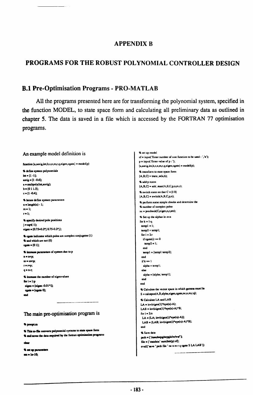
APPENDIX B
PROGRAMS FOR THE ROBUST POLYNOMIAL CONTROLLER DESIGN
B.l Pre-Optimisation Programs - PRO-MATLAB
All the programs presented here are for transfonning the polynomial system, specified in
the function MODEL, to state space fonn and calculating all preliminary data as outlined in
chapter 5. The data is saved in a file which is accessed by the FORTRAN 77 optimisation
programs.
An example model definition is
I'wx:tion [a,lOI'ia.int,b,c,n.m.r,q,cigcn,caatej .. model(p)
Ii dDfiDD I)'IICm polynomiall
1m- [1-1);
IIIria • (1 -0.6); a • multpoly(inl.aori&>; b. [0 11.5);
c • (1 -0.4);
Ii DlIIIlO dDrlDD IYStcm parameters
D .lrmat\lCa) - 1; m.1;
r.1;
lilp&Cify dDliml pole pDlitiOlll
j -1CJ(-1); oipD. [O.75+0.2-j 0.7S-O.2-j);
Ii cpIII indicaIDI which polu ue complex COIIiUplCl (1)
Ii IIId which arc 1101 (0)
cpIII- [0 1);
Ii ___ ....... 1Dn of Iystmn chao to p
D.D+p;
m.m+p;
r-r+p;
q -n-r;
.. ___ h IIWIIbar of CiacnvalllOl
fDrl-1:p oipD. [oipD -O.OI-i);
..... ( .. 0);
and
The main pre-optimisation program is
"JRGPl.m
.. 11111 m-!IIe axwona poIyncmial IYS_ to IIaID IJIMlO ronn
.. and _ h cllta twqIIinId II)' h ronran apIlmiaaliaD JIIGIIWN .. ........... • -1,·10;
Ii sci up model
cC = input( 'Enter mllnbcr of coli funclion \0 be IIICd : '''e');
p = input( 'Enter value of p : ');
[a,aoria,inl,b,c:,n.m.r,q,cip,c:aatel- model(p);
Ii transform to state .paa: form
[A,B,C! = tranI_n(a,b);
Ii add P states
(A,B,C! • add_IIIIC(A,B,C,p,n,m.r);
Ii Iwitch >tate. 10 that C .. (I 01
(A,B,C! = Iwitc:lJ(A,B,C,p,n);
Ii pcrfonn some limple chew and dctennine tha
Ii number of c:omplc:x poles
nc '"' precheck(C,cip,ll,r,llll);
Ii Set up tha alphas in uta
Cork = I:q
tempI = I;
temp2 = tempI;
Cor i = 2:r
if caalC(i) = 0
temp2= I;
end
tempI .. (tcmpltcmp2);
end
ifk= I
alpha = temp I ;
elle
alpha = (alpha; tempI I; end
end
Ii Calculate tha vec:lor space in whi=h prnrm JIIIISt liD
S .. c:a\c:spce(A,B,a\pha,cipn,c:,a.,nc:,n,m.r ,q);
Ii Calculate LA IIId LAB
LA - inv(ciactl(1)"yc(n)-A);
LAB = inv(ciacn(1)"yc(n)-A)·B;
fori - 2:n LA D [LA; inv(ciaaJ(i)·c)'C(D)-A»);
LAB • (LAB; inv(ci&cnCi)·~n)-A)·Bj;
end
Ii Save data
path. ('~Jllkdw/W"'); rile • ('ImIdata' nurn2aIJ(p) cf):
oval« '.ve ' path mo ' nc D m r q C&* S LA LAB 'J)
- 183-

The associated functions are
fiuII:&iaa (A,B.CI • traaJl(a,b);
.. fiuII:&iaa to traafarm II1II ~ poIynamiall to Ilalc SJ*'C
.. ot..v .... c:GIOIlicU farm - Opla, diacrcte time c:oaIroI. p491
... Jm&tb(.);
Ib - Jm&tb(b);
.. ifb • lower weier than a, IIIIIn pad b wilb zcr .. fori-1:1b
aupb(i) • b(i);
CIIId
iflbc" forl.1b+1: ..
aupb(1).0;
CIIId
Ib -1a;
CIIId
.. nmA MATRIX
.. -lcadin& 1 in. polynlX'niai
1IImp& -1(2:1.);
1 .... -1;
.. c..... A wi!how lUI c:olwm of. poly c:ocfficicnt. A • .,.,o.-l): •• _CII(1).-I);
A-(a; A):
.. IWltd! ardIII' IUId IIIIpll:o • poly c:ocfficicnt.
for i .. 1:1.
lIImp(i) - -1iDInp&(1.+ 1-i);
tIIId
.. add.poIy c:ocflil to A malrix A. (A 1Dmp');
.. nmBMATRIX
.. calc B e1011101J1a - don't \lie bO IOlb = Ib-I
Ib.1b-l;
B SlDrol(lb.l):
fori -l:lb
B(I) .1Dmpb(1b+2-i) -l(lb+2-i)-lempb(I);
CIIId
.. nmCMATRIX C. -..(1).-1); C_(C 1);
IImc:tIoa (Al.Bl.Cl) .1dd... .. ID(A.B.C,p.n,m,r)
.. ftmction to aupllllllllllllayalllm wilb p exira staleS
.. 1IDIII1I,m,r haw all bad P Iddcd for eXira stales
lpIi!aa-O;
.. nmAMATRIX
Al • (A -..(n-P.p»): AI- (AI; ~,n-p)epailon·e)'a(p»);
.. nmBMATRIX
81 - (B _CII(n-p,p»);
81 - (Bl; ~.m-p) eye(p~on·e~(p»);
.. nmCMATRIX
Cl • (C -..(r-p,p»);
Cl • (Cl i -..(p,n-p) eye(p»);
6ux:tIaa (AU1.Cl) - Iwitcb(A,B.C,p,Il);
.. ftaDI:tiaD to IWilch IhD ltallll ludllhDt C 111 allhD tGIID (I 0)
....... dlat C II in II1II abaDrYabIo CIIICIIIic:aI t_. 1 .. 10 I)
.. nmAMATRIX
.. IwItch IOWI. IhDD coI_
"IOWI
AI- (A(.pcD,:); A(I:o-~I.:)J; .. coI_
AI - (A1(:,II-p:Q) Al(:,1:11-~I)J;
.. nm I MA11UX
....... IOWlllllly II _18(1a-p:a,:); 8(1:81'"1,:»);
'10 TIlE C MATRIX
'10 .wilCb colwms only
CI = [C(:,n-p:n) C(:.I:n-p-I»);
function numc:an = prccheck(C,cip,n,r,small)
.. function to perform some simple c:hc<:b and to
'10 dclennine the number of c:omplcx pole:.
.. check lhalthe com:ct number of cigcnvallll:S ha~ bcc:n ipOCiflDd if D -= length( cip)
Drror('lncom:a number of ~irlCd cigcnvallll:S')
end
.. check C is of the correct form
chid = (cyc(r) zcros(r.n-r»);
cbk2= C - c:hkl;
if .wn(awn(cbk2 > small» > 0
Drror('C is 1101 oC the corrcc:l Corm ');
end
'10 dclCnnine number or complex CiacnYalllCI
nlUtlC(JfD = Iwn(imal(cilcn) -= 0);
'10 check if all cilenyalllCl arc complex
if numclX'D ... D
crrar('AlI poles arc complex')
end
function lSI • calCSPC;C(A.B,alpha.cip.claU:,nwnclX'n,n,m.r.q);
.. function to calcula'" zeta Cor real and complex pole.
'10 will nol work Cor all complex cue
'10 CAl..clJLA TE ZETA
counl = I; Cori=l:q
Cork = I:r
II = (inY(ciac:n(i+r)'cyc(n)-A)-illv(ciacn(k)'cyc(n)-A»"B;
II = alpha(i,k)'II;
iCk=1
a = 11(1:r,:);
cllC
a. (al1(l:r.:»);
end dear t1
end iCi=1
zeta = t2;
clsc
zeta = (zeta; 12);
end c:Icar a
end
iC nlUtlCom > 0
.. SOME POLES ARE COMPLEX
.. calc:u.lllic IICtabr by n:movina ~x conju .... row. mel col •
.. dcll:onnine which row ..... c:ompIcx COIIju ..... dDJaIdanI GIl
.. II1II ciacuvalun UJocilu:d wilb P2 (i-O r+l • n)
liClU = liCtI(l:r.:);
for i. 2:q
if cpu:(i+r) .... 0 .. cilcuvaluc ill nol I CDqIIex conju .. u: 10 _ row block
IICIU II [lICtal; .tI(l+(i·I)~I+(i·n-r+(r·I).:)I;
end end
.. dcu:nninc which cola .... c:ompIcx conju ..... dDpcndanl em
.. \he CiacnvalllCl usoc:iau:d wiIh F1 (iA 1 • r)
llltab = IICtaI( :.1 :m);
fori·2:r
if cplc(i) - 0 .. cipllval\ID IIIl10ll c:ompIca COIIjllpID 10 _ cal block
..tab _I_tab .... :.1 +(i-l) .... : 1 +(i-l) .... +(-I))J;
.ad
.ad
- 184-
AppendUB

,. calc:Wa1e 7A11abr, tbc _ part of zctab
7AIIabr - n:al(JJeIab);
,. 7BTABI AND ZETAGJ HAVE TIlE SAME NUMBER OF ROWS AS ZETAA
,.lIIIabi
COII.l:q
II (cptII(i+r) = 0)
1IImp1 '"' iDv(0iacn<1)~) - A)-B;
1IImp1 '"' upmci,l)-limIpl(1:r,:);
COl It • 2:r
lI(cpID(k) -0) ok (imq,(oip(k»> 10-12)
1IImp2 '"' iDv(oipn(k)~) - A)-B;
...,1. (1Dmp1 upbl(i,k)·tcmp2(l:r,:»);
...s ...s 1I1IIIIJ(.~tabi)) = 0
.tabi. imlaClllmpl);
01_
zetabi'"' (zolabi; ima,(templ »);
ODd
ODd
ODd
,. zoIa&i - nnt c:olurm
tempi .1nv(oipn(l+r)·oyc(n) - A)+B;
tempi '"' tcmpl(1:r ,:);
COl i -2:q lI(epIID(i+r) .. 0)
temp2 .. Inv(oipn(i+r)·eyc(n) - A)- B;
....,1. (!llmpl; temp2(l:r,:»;
ODd
ODd ....,1. ima,(lIImpl);
ZlllaIi .lIImpl;
for I. 2:r
II (cpIlD(i) - 0)
-lali - (zelaai tempi);
ODd
end
,. bDlIIlO zola
(tl,ll) - .izo(zolall);
(13,t4) - .iza(atabr);
(tS,16) - .'-<zetabi); zeta _ (zolabl; ~13-tS,I6»:
zoIa - (_labr _lal: zoIa - (_la; zotaal zorOl(ll,t6+t4-t2»;
.. dIlOlD ..-0 row. IIId c:olurm. frorn zeta
"row. flHt
flnlMrorow - 0; 1-0; whilo (rantzcrolOW -0) oft (i < 11 +13)
'-i+l;
1I1Il)'{M1I(i:i,:» - 0
" zero row flrsu.crorow = i;
end
end
if flrsu.crorow > 0
" check 1Cl1l&iDin, roWI an: all zero
for i = flrltZCrorow+ 1:11 +13
if lIIy(zcta(i:i,:» = I
" non zcro row crror('mW:d zero rowl in zetl')
end
end
,. delelC roWI from zetl
ZCtI = zeta( I :flrllZcrorow-l,:);
end
" now wlumns flrllZOrowl = 0;
i=O;
whae (flnlZenx:01 =(0) &: (i < 14+\6)
i=i+l;
if lIIy(zctl(:,i:i» = 0
" :rcro col flrltZCrowl = i;
end
end if flrl\Zerowl > 0
" check rcrnainin, wI. an: all zcro
for i = flrllZOrowl+ I :14+16
if lIIy(zcta(:,i:i» = I
" non zcro col error('mixed zero wI. in zetl')
end end
" delete wI. from zetl zeta = zeta(:,I:fll'lrunx:01-I);
end
end
" CALCULATE TIlE NUU- SPACE OF ZETA
S = nllll(l.cta);
(11,121 = .W:(S);
if 12 < r+(m-q)
byboud errore '1110 mall spaa: of zeta is till: wrona cIiIncnaioo ')
end
- 185-
AppendUB

AppendUB
B.2 Optimisation Programs - FORTRAN 77
All the routines associated with the numerical optimisation itself are written in FORTRAN
77 to facilitate the use of the Numerical Algorithms Group (NAG) library routines. Because the
parametric state space design has to be performed during the calculation of the cost function a
number of additional programs have had to be written, also outlined in chapter 5.
The main optimisation program and its associated
routines are in the file J AF.F
C JAP.P
C Defme panmDtcn C (NN • 110 of variables = r"(m-q)+q)
inlDprPNN
cbandcr°IP panmDtcr (PNN .. 13. P = '3')
C Deline panmDtcn ioIDpr maxn,nwun,maxr ,maxq,maxsr.maue.nwn
C (mun,nwun,maxr,maxq - maximum values of panmDtcn of system)
C (JDalW,maxsc - maximum dimension oC S. r(m-q). r(r-q»)
C (1IWI1- number or errcrs beina considered)
panmDtcr(maxn =10. maxm =9. maxr = 9. maxq = 3. num = I)
panmDtcr (muir = 81. maxse = 81)
C CcImmon ac:a1an inlDpr nc:,n,m.r .q." .IC.count.ltore
double pnc:ision aPC dwac:terol Nl
cbandcr0 30 FNAME4
C CcImmon arrays inlDpr COA'rn(maxn) doublo precision S(maxsr.maxsc).WEIGHT(3°maxn)
double complex P(maxm,maxn).V(maxn,maxn).W(maxn.maxn).
° LA(maxn,maxn,maxn),LAB(maxn,maxn,maxm).
° KC(maxm.maxn).dA(num.maxn,maxn).
° d8(num,maxn,maxrn)
C CCIIIIIDDII b10da common /CONSTII count .. ton:o.nc:,n,m.r.q.sr.sc.NI ,FNAME4
COIIDIIOIl /CONST'1I CGA TE.dA.dB.WEIGHT.LA,LAB.S. KC
common /RESULTI p.V .W ,aPe
C Local ac:a1an iDIapr lJ,NN,L1W ,LRW .IBOUND.IFAn.
cIoubIe precision PC.FO>RIG
11llic8l OK
c:baraeIiDr°l ANS,FNUM c:baraeIiDr"30 FNAMEI ,FNAME2,PNAME3
C Local arrays. (1W(>NN+2).X(NN).RW(>120 NN+NN(NN-I)/2»)
..... 1W(100) dDubIo preciaian X(PNN).xORIG(PNN),RW(SOOO).BL(PNN).BU(PNN)
daubIo camp/ll1I VORlG(IIIUII,ID&xn).KCORIG(JIlIlUJI,IIIaxn).
• PORIG(maxm,maxn)
C Ded_ ....... 1UlIprapams
....... PUNcr1
C SaIec:t COIl flacDioD priaI.,' , priaI •• 's-COIl fuDI:tian IIIIIIIbar (in .-a>' ..... NI
C .... tbt inIIW,.--- hili m. (nppliDd by MaIIab)
PNAMBla ....... 11.-&·
PNAMB1(1:1) • P PNAMB1(9:f) • Nl lID RDATA(PNAMBl.s .. ,ec,LA,LAB.COA~N
C Check NN is sel to Ihc com:c:t value
NN=PNN if (NN .nc.(r"(m-q)+q» Ihcn
print·. 'PNN should be acito • ,(rO(m-q)+q)
Ilop
end if
C Load l\art dala
FNAMEI = 'cosll/llUldatall.maI'
FNAMEI(S:S) = NI FNAMEI(16:16)" P
FNAMEI(l7:17) .. NI call RSTART(FNAMEI.x.dA,dB.WEIGIIT,NN)
C Selup paramcICn - scalan
OK=.TRUE.
lBOUND= I
counl"O IIOIC = 99
FNAMEI .. 'cosII/JAFlori,1 I.mal·
FNAME2 = ·COSII/JAFlopI....ll.m.l·
1'NA. .... E3 = ·JAFImp_orig.maI'
FNAME4 = ·JAFtmp_opl.mal·
FNAMEI(S:S) = Nl
FNAME2(S:S) = NI
FNAMEI(1S:1S) = P FNAME2(lS:IS) = P
FNAMEI(l6:l6) = NI
FNAME2(16:l6) = Nl
C Sel up paramcICn - arr.y dimensions
LIW= 100
LRW=SOOO
C Siore £roe paramcll:n
dol=I.NN XORIG(I) = X(I)
caddo
C CalculalC criginal value or costf unclion print· •• ,
print·. 'Original values' call FUNCTI(NN.xORIG,FCORIG)
C Siore criginal values or V and P
do I = l,n
do J = l.n VORIG(I) = V(I)
end do
end do
dol .. 1,111
doJ = I.n PORIG(I) • F(I)
end do
end do
call CALCKC(n,m,P.W.KCORIG)
C Siore cri&iu\ data in ICl1Iporvy file in cue propam abcnId call WORJG(NN,m,n,FCOllIG.XORIG,PORIG.VORIG,KCORIO.PNAMD)
- 186-
print· •••
pride,' •
prid·. 'P'1DiIhod .. up'
prinl· •••

dowbie(OK)
IPAIL-I
c:a1l B04JAP(NN.IBOUND.BL.BU .x.R:.IW.LIW ,RW.LRW .IFAIL)
pr"-,' • ....... 'Ori&iual Value : •• R:ORIG
....... 'Weipted 0pIimaI Value: '.R:
........ Ac:IuI 0pIimaI Value : ·.aPe prial* •••
c:ount-O _-99 ....... 'FmaI values'
c:a1l PUNCTl(NN.x.Fc)
OK-.PALSE.
it (JPAlL.eq.O) tbDn
....... 'B04JAF bu found a minimwn point. •
ebeit(IPAIL.cq.l) than
....... 'Par_outofranF.'
aile iC (IF A1L..aq.l) tbDn
... int ... '400"NN fwx:tion evaluatiOlll'
print·,' •
... int ... 'Reltart with aid X (yin) 7'
~d·.ANS
iC «ANS..aq. ·y·).or.(ANS.eq.'Y·» than
OK-.TRUE.
ondiC
0110 iC(IPAIL.cq.3) than
... int·. 'The oonditions for a minimwn ha \Ie not all been'
... im". • .. tilflCd. but a lower point could not be found .•
0110 if (lFAIL.cqA) than
... im·. 'OverfIow haloec:urod'
... im ... • •
... im". 'Rostart with aid X (yin) 7'
~".ANS
Il «ANS..aq. ·y·).or.(ANS.eq. 'Y'» then
OK-.TRUE.
ondif
ondll prinl*, ••
... im". 'Save current parameter values (yin) 7'
~d·.ANS
Il«ANS..aq. ·y·).or.(ANS..aq.'Y·» then
... im". 'Bntar rile nwnbcr (in quotel)'
_d".FNUM PNAMBI(lO:IO) • FNUM PNAMB2(IO:IO) .FNUM call WORJO(NN,m,n,FCORIG.XORIG,FORIG.VORIG.KCORJG,FNAMEI)
call WOPT(NN,m,n.PC.x.dA.dD.WEIGI-IT.F.V.KC.FNAME1)
and If ... in1 ... ' •
and do
IIIbroutino PUNCTI(NN.xC,FC)
C Subroutine 10 c:aIc:ula. tha value of tha objoctiwe function
C _lduaIs
C Den.. panmDlOn
..... _,aaxm,mur,maxq,maur ,m1llllC,mUCCIIlnt,n1llD
C (_,aaxm,mur,muq • muilm&m vaI_ 01 parunctcn of system)
C (_ • JIIIIIIbIIr of III1'OrI belna _idDrod)
C (_.-.1MIlimwn dirMnaian of S.I(m-q).I(r-q») ..-_ (_. 10. DalIIII • II. mur • II. muq .3. DIIII .1)
..-_<_ .11. muac:. II)
..-_ (mucount. 20)
CC-..... ..... sAfl¥,q, .... -t,11Df8
...... preciIIaD aPe
........ lNl
......,.PNAMBC
C Common urays
inlcacr CGA TE(1NXJl)
double precision S(maur,DaXX).WEIGI-ITO.IDUD)
double comple" F(nwun,mun).V(mun.mun).W(mun,mam),
• l.A(mun.mun,mam).LA8(IlIaltIl,InaltD),
• Kqrnurn,mu.n).dA(I1WIl,DWlD,IIWa),
dD(nwn,mun,mum)
C Common blocU
common /CONSTI/ colDll,lkm:.DI:,n,m.r.q.sr.II:.NI,FNAME4
common JCQNST1I CGATE,dA,dB,WEIGI-IT,~B.s,KC conunon /RESULT/ F,V,W,aPe
C Scalar ugwncnIJ
integer NN
double precision PC
C Array ugwncDlS
double precision xqNN)
C Loca1 scalars
integer I,T
C Loca1 urays
double precision V AL(mun),VEC(mun).VECSEN(num.mun)
double complex V ALSEN(nulD,mun)
C Declare externsllubproarams
external DALEY,COSTI,COSTl,COSTI.COST4
C Calculate OUtpul Cccdbac:k IISing appropriate melhod
call DAl.EY(NN,xC,S .. r,sc,LAB,CGAlli,DI:,n.m.r,q.F,V.W)
C Calculate K
call CALCKqn.m.F,W,KC)
C Calculate COli function
if(NI.eq.'I') then
C Eiaenvaluc diCCercnliaJ coil fuDl:lion
call COSTI(n,m,V,W,KC,dA,dB,WElmrr,pc,aPe,VALSEN)
else if (NI.eq.'2') then
C EigeDllrUclUrc diCCerentiaI COlI function
call COST2(n.m,F,V, W ,KC,tA) .AB,dA,dB,WElmrr ,FC,aFC,
V ALSEN,VECSEN)
elsc if(NI.eq.'3')then
C Transient leSpanlC dirrcrcnlial COlI function
call COST3(n,m,F,V,W,KC,tA,LAB,dA,dB,WEIGI-IT,FC,aFC,
VALSEN,VECSEN)
clac if (NJ.eq.'4 ') then
C Cundilionina COlI funclion
call COST4(n.V,W.WEIGm.rc,a1'C)
elac
print-. 'No othor COlI functions )CI'
slop
end if
C Prinl PC .lIer acl number or itcnlions
counl = COIIDI + I
if (counl.gema"colIDl) 1hen
counl=O
prin'-, PC,' ',aFC
end if
C Slore mes aller 100 ilCralions
slore = slore + I
- 187-
if (1IIR.,e.100) then
slore = 0
call WOPT(NN,m,n,PC.xC,dA,dB.WEIGlrr .F.V .KC,FNAME4)
)X'inl-, • t
print·. ·S.wed data in IcIl1' mo' prina-, • I
prilll·, PC,' ',aPe pin&.- I • ,
iC(NI.nc.'4') then
... inl", 'Eipnvalue SoIIIitiviticl'
dol.l.n
VAL(I).O.O
doT-I.llllm
VAL(I). VAL(l) + .. aqr(1NI(V ALSEN( 1.1)·canja{V ALSBN(1 ,I))
and do
oncIdo
p-_ 10,(VAL(I).I. I.n)
p-_ 10,(WEIGlml)·VAL(I).I-l,n)
AppendixB

if «NI.cq. '2').ar.(NI.cq.'3 '» li&n
pr ... , 'BiFn~ Sen.itivilie.'
do 1-1,11
VEC(I)-O.O
doT-I,DWD
VEC(I) - VEC(I) + VECSBN(T,I)
Cllddo
auddo
pro. 10, (VEC(I),I = I,n)
pro. 10, (WEIGIrr(l + 2·n)·WEIGIrr(l+n)·VEC(I),1 = I,n)
Clldif
10 lomw(IOOI2A)
I1&broutinD CALCKC(n.mJ',W,KC)
C SubroutiDo to calc::lIlatc Ii& alp feedback malrill
C Define JlUUllDten
inlDpr _,mum
JlUUllDIIIr (IIWUI = 10, maxm = 9)
C Scalar argllllllmll
_prn,m
C Anay argumenta
double c:omplDll F(maxm,maxn),W(maxn,maxn),KC(maxm,rnaxn)
C Loca1 .cal_
integor I,J,K
C c.1c::ulatc KC, millt F and W
do I-I,m
doJ.I,n
KC(I.J) = dc::mpbt(O.O.O,O)
do K -I,n
KC(I,J) - KC(I,J) + F(I,K)·W(K)
auddo
and do
IIDd do
rctwn
IIDd
The parametric state space design is performed by the routines in the file DALEY.F. This includes the routines
for the calculation of an accurate inverse and the null space of a matrix via the singular value decomposition (SVD)
I1Ibro1IIinD DALBY(NN .xc,s .. ,Ie:,lJ\B,COA TE,nc::.n.m,r.qJ'.V.W)
C DIIIy'I _Ibod fIl o/p fDcdbaclc: dc.ian
C DefiDI JlUllllDIIIn inlDpr 1IIUII,mum,mu .. ,max.e:
cIoubIo pnc:Iaian _0
C (_,mum -muimwn valllCl oCparanaten oCly.tcm)
C (-,IIIUIC -muimwn climcnion fIl S.I(m-q).I(r-q»
JIUIIIID- (mun - 10. mum - 9)
JIUIIIID'" (_ - 81. maue: • 81)
JIUIIIID- (_10 - 0,0)
C War...-_ .. NN .. ,II:,II,IIl,r.q.nc
C ,..., .........
..... COA113(-a)
cIoubIa ...... XC(NN).S(mu_'->
........ -.Ia. LAB<mun,mun,muIa).
• P(mum,mun).V(IIIUII,IIIUII),W(mun,lllUll)
C LoaII ..... ..... I.J.K.DIM.RANK
C Loca1 array.
dollble p-c::c::ision GA.\t\fA(maxsr),spcr,(maxm,llWUll),
• ~1D&JUD.mum)
C c.1culalC pmma &1lOJ Ibc nllll ,pace: of zcla
dol=I, ..
GAMMA(I) = 0.0
do J = I,ac:
GAMMA(I) = GAMMA(!) + XC(J)"S(I)
cnddo
end do
C Exlral:t FI from pmma
call CALCFl(GAMMA,COA TE,nc::,n,rn,r,q.F)
C c.1cu1alC Ii& fU"JI r \ICC"'" of V
dol = I,r
doJ=I,n
V(J,I) = LAB(I),I)"F(I,I)
do K =2,m
V(J,I) = V(J,I) + LAB(I),K)"F(K,I)
cnddo
end do
end do
C c.1cu1alC Ii& remaining F \lCctan
C A.IWIICI that all poICi auoc:iatcd with F'2 _ n:aI
do l"I,q
C Cale:ulalC Zi u a real malrill
c:aJ1 CALCRZ(LAB,F,V,I+r,rn.r,RZ.l
C Find the nllll space: of RT
c:aJ1 CALCSVD(RZ,rnaxm,rnaxm,m,m,DIM,RANK,s~)
if (DIMJt.l) then
print·, 'Error in DALEY'
prillt·, 'No 111111 space: ex i .... for ,,'
'top end if
C IlpdalC F· UlllffiCl all poles UlocialCd with F2 _ n:aI
doJ = I,m
F(J,r+!) = dcmplx(XC(r"(m-q)+I)·SPCE(J,I),-o)
cnddo
end do
C CaicwalC the remaining V YCC\(JIS
dol =1+1,0
doJ .. I,n
V(J,I) = LAB(I).I)"F(I,I)
do K .. 2,m
V(J,I) = V(J,I) + LAB(I),K)"F(K,I)
end do
cnddo
end do
C c.1cu1alC W = iov(V)
call CALCINV(V,W,maxn,n)
relllm
end
Ilibrolitine CALCF! (GAMMA,CGA TE.nc,n.m.r,q.P)
C Silbrolitinc 10 ClItract the P! \lCc:un Crom pmma for rcaJ or
C c:omplDlt polol
C Scalar arglllllCDlll
integer n,m,r,q.nc
C Ana" arglllDCllll
-aer COATE(IO)
dollble ~It P(9,10)
dollble prociaian GAMMA(81)
C LcallQIJus
inIIIacr I),POSREAL,POSIMAG double proc:ilicIIl1ERO
C LcaI arraY'
- 188-
AppendixB

C Oem. .wtlua poilU
POSREAL-O
POSIMAO-O
do I-I"
if (OOA "ffi(I).eq.O) then
POSIMAO - POSIMAO + m
mdif ClDddo
C Due fA) ordDriua ofpolc let (i.e [~Icx real», we know C lbat the rD'. 1IIIIDC~lcx po1ca _ compJcx
C complex po1ca rn do I - 1..,,2 doJ-1,m
FQ,I) .. CMPLX(OAMMA(J+POSREAL),GAMMA(J+POSIMAG»
pu,I+I) -CONJG(P(J,I»
aaddo
POSREAL. POSREAL + m
POSIMAO - POSIMAG + m
ClDddo
C Now real po1ca lBRO.O.O
do 1-111:+1,1
doJ .. 1,m
pu,I) = DCMPL.X(2.0·0AMMA(J+POSREAL),ZERO)
IIIJd do
POSREAL - POSREAL + m
CIDd do
IUbroUlinD CALCINV(A,B,MAXN,N)
C IUbroutinD fA) calculate the inverIC of a complex matrix A
C UId ltore the !eIIull in B
C Scalar araumclll8
_pr N,MAXN
C Array argwncnll
doublo compJcx A(MAXN,MAXN),D(MAXN,MAXN)
C LocaJ lcal_
_prl,J,rrS,IPAn..,ID
double pnciIlm D 1 ,BPS
C LocaJ uraY'
cIoublo prociaillll RA(20,20),AA(20,2O),RB(2O,1 0),BB(2O,10),
• RHS(20,10),I'(2O)
C Dod_ cxlDmal functions
cIoublo prociaion X02AAP
C DIIIrmino BPS
BPS - X02AAF(O.O)
C Sot up .-1 matrix RA colllilting of the real and imaginary
C ,..,.or A
do 1-1,N
dol -l,N
RA(I» - ..J(A(I»)
MCI» - RA(I» RA(I,J+N) --dImaa(A(I))
MCI)+N) - RA(I)+N)
RA(I+N» - dimq(A(I»)
MCI+N» - RA(I+N»
RA(I+N )+N) - ..J(A(I,J»
MCI+N)+N) - RA(I+N)+N) _do
_do
C Sol up tho ,... ..... 1idD CXlllliIIlIIa or tbo NxN idamay C matrix IDd a .ro Woc:k
eID 1-1,N
elDl -1,N
if (1.eqJ) then
RHS(I,J) - 1.0 .. RHS(I,J) - 0.0 _If
RHS(I+N) = 0.0
cnddo
cnddo
C SOLVE RA.RB = RHS
C Paaoriac: RA inIo upper and lower tnincJulat matric:a
IFAIL= I
call FOJAFF(2·N,EPS,AA,2O,D1.ID.P,IFAn.)
if (IPAR...nc.O) Ibm
p'int·, 'Error in CALCINV'
p'int·, 'P03AFP failed to find. soIn, IFAIL = ·,IFAn.
IIop
end if
C Salve equation to rmd invcnc
IFAIL= I
AppendixB
call F04AHF(2·N,N,RA,20M,2O,P,RHS.20,EPS,RB,20.BB,20.rrs,
• IFAIL) if (IFAn..nc:.O) then
p'int-, 'Error in F04AHF'
llop
cndif
C Extract real and imaginary pans from RB
dol = I,N
doJ=I,N
B(I,J) = QIIp1xCRD(I),RD(I+N))
end do
end do
rcluMi
end
lubrouliD: CALCRZ(LAD,F,V ,II,m.r,RZ)
C Subroulinc 10 c:alClilatc RZ
C Auumcs lhalthe poles usoc:iatcd with F2 arc real
C Define parunctcn
integer maxn,maxm
double p'cciaillll zero
C (malUl,nwtm' maximum value. ofparametcn ol'lY'tcm)
C (zero. maximum value for a number to be COIlIidared zero)
parameter (1IWUl .. 10, maxm .. 9)
paruncter (zero = le·IO)
C Sc:alat atgwocnll
inteacr lI,m,r
C Array argwncnll
doublo prociaion RZ(maxm,maxm)
doublo complex LAB(IIWUl,DWID,nwtm),
F(maxm,DWID),V(maxn,rnaxn)
C LocaJ aca1an
intelIII' U,K
C LocaJ uraY'
double complex iVII(IIWUl,DWID),2(maxm,IIIIIlUD),n(maxn,maxn)
C Calc iVII
call CALCINV(V,iVII,DWID,r)
C Calculate Fl-iVII, resull in TI
dol.l,m
doJ .. 1,1
n(I,J)-o.o
do K = I,r T1(I,J) .. n(l,J) + F(I,K)-iVII(K)
cnddo
cnddo
end do
C Mullresull by LAB, !eIIul1 in Z
dol=l,m
-189 -
doJ.I,m
1~1)-0.0
do K -1,1 ~I) - ~I) + Tl(l,K)-LAB(II,K)
end do
end do onddo

c Sublnct JaUlt tram _Dtity marrix 10 Jive Z
."1,111 .J-l,m
if (I.eqJ) bn
7.(1) .. cIcaIplx(l.o,O.O) - 7.(1)
cbc
7.(1) = -7.(1)
and If
C a-It imI&irary put is zero IDd -ian RZ If (dlmaa(Z(I)).&Lzcro) bn
prial., 'm.,inary put of Z is not zero'
p'inl· , dimq(7.(I))
IIop -RZ(IJ) - JNl(7.(I))
and if and.
and.
nbroutine CALCSVD(A,AM,AN .M,N,DIM,RANK,SIU)
C Subroutine 10 calculate the null or ranac space oC a marrix
C lIIma the svd, which is calculated by fll1din& the ei&cnveclon
C ofA·AtandAt·A
C Define puamet.en - (maximum dimensions of A)
iDlDaor maxm,maxn
pumlD1Dr (mum. 50, maxn .. 50)
C Scalar arcurnmta
iDlDaor M,N,AM,AN,DIM,RANK
C Array arcurnmta
double p-eciaion A(AM,AN),SPCE(AN,AN)
C Loc:aI sca1an
iuII:&er I), K,IP AIL
double p-eciaion BPS,TOL
C Loc:aI array.
double p-ecisiOll AT(maxn,rnaxm),AA(maxn,maxn),
• V(maxn,maxn),EIG(maxn),WKSPCE(maxn)
C Set Dp&ilon the smallest number
BPS -lB-7
C find IrINpO& DC A
dol-I,M
dol-l,N
AT(J,I) - ACI)
aad. aaddo
C c.Jc:V,rmclA'·A
do l-l,N
.J-l,N
AA(I)-O.O
doK -1,M
AA(I) - AA(I) + AT(I,K)·A(K)
aaddo
oneIdo ead. C find _rrix ofrlahleipnvec:lcn - V
FAIL-I CIIl F02ABF(AA,mam,N,BIG,V,mull, WKSPCE,IPAIL)
II (IPAIL.IID.O) dan
p'1nI., 'Brror in CALCSVO'
...... , 'Pailed 10 lind thD eipnllnlCllln of AlA'
IIap _II
C c.J ..... da rut -.... OIIeipnval_ wblc:b _ thD
C ... of ... "alar YIl_. 1'hlI_1O live bDWlr
C -aI.1II11 1'01. - ..x(M,N)·IIpt(EJO(N»·BPS
RANK-O .I-I,N
1I(B1O(1).,at.BPS) ....
1I(...,u~I)~11)L)thDn
RANK = RANK + I end if
end if
end do
C Return the null spea: of A
do I = I,N-RANK
doJ = I,N
SPCE(J,I) = V(J,I)
end do
end do
DIM=N -RANK
~turn
end
AppendixB
The cost functions and all associated routines are in the file CFUNC.F
subroutine COST1(n.m,V.W ,KC,dA,dB, WElmrr ,FC,aFC,V ALSIiN)
C Subroutine 10 calculate II .. COlt runction balCd on ei&envalua
C ICnsitivities
C Define parunclCn
integer ... axn,mllJlm,nurn
C (maxn,maxm - maximum val .... of parunct.en olsy.t.em)
C (num - number DC etTora beina considcrod)
paruncler (maxn .. 10, mum = 9, Dum -I)
C Scalar argumenLl
inrcger Il,m
double precisian PC,arc
C ArrayargwncnLl
double precisian WEIGIIT(3·maxn)
double complex V(maxn,maxn),W(maxn,maxn),KC(mum,mun),
• V ALSEN(num,maxn),dA(num,maxn,maxn),
dB(nwn,maxn,maxm)
C Local scalan
inteaer I,T
double precision TE MI)
C Calcularc oigenvalua ICnsitivities
call EIGVALCn.m,V,W,KC,dA,dB,VALSEN)
C Calcularc ~iduall
pc .. o,o arc .. 0.0
dol=I,n
doT= I,Dum
TEMJ> = ~al(V ALSEN(T,I)·conjg(V ALSEN(T,I»)
PC = PC + WElmrr(l)-TEMJ>
aPe = aPC + IEMJ>
end do
cnddo
~tum
end
subroutine COST2Cn,m,F,V, W ,Kc,LA,LAB,dA,dB,WEIGHT ,PC,IPC,
• VALSEN,VECSEN)
C SllbroUlinc to calculall: the c:uIl function buDd 011 eipwaI
C and oigcnveaor lOIIIitivitiea
C Denno pararnot.en
inlcaer 11l&lIII,maxm,num
C (mam,maxm-maaimwnval_ol .......... ol.,-m)
C (_ - IlIImbor 01 CI1'OI'I -ina coraidDnldl
pumlDlIIr (IIIUD • 10, maam - 9, IIIlIII • 1)
C Scalar araumenu
inleaer n,m
double p-eciaiaa PC,afC
-190 -

C AIrrf.,.-double JRCiaiaa WEIGHT(3'mun),VECSEN(DIUII,IIWUI)
double c:ompIDx P(mum,mun),V(mun,mun),W(maxn,maxn),
• • •
LA(1IW.1ID m'm,mun),LABCIJIUJI,IIWUl.,R),
KC(mum,mun),V ALSEN(nwn,maxn),
dA(nwn,maxn,maxn),dB(nwn,maxn,mum)
C LocaIIC:aI ..
_prlJ,T double JRCiaiaa PCl ,aPCl,PC2,aPC2, TEMP ,NORMV ,NORMW
C Local uray. double complex VSEN(mun,mun,mun),WSEN(nwn,maxn,maxn)
C Calc:u1all: cipvaiuc lCIIIitivitiA
call EIGV AU.nlD,V ,W ,KC,dA,d8,V ALSEN)
C Calc:u1a11: cipnvcc:t« lCIIIilivilic.
call EIGVBC(n,m,P,V,W,KC,LA,LAB,dA,dB,VALSEN,VSEN,WSEN)
C Calc:u1a11: the DOmUI or each acl of lCDIitivily vecton
dol-l,n
do T = 1,IDIID NORMV=O.O
NORMW .. O.O
doJ .. l,n
NORMV - NORMV + (rcaJ(VSEN(T) ,1))"2.0 +
• dimaa(VSEN(1' ),1)"2.0)
NORMW .. NORMW + (reai(WSEN(1',I))"20 +
• dimal(WSBN(1',I))"2.0)
cnddo
VECSEN(T,I) .. cllqrl(NORMV) + diqrl(NORMW)
IIIUI do
IllUldo
C Calc:u1all: function· ei,cnvaiuci
PCl.O.O
&PCl .. 0.0
do I-l,n
do l' • l,lDIID TEMP -11Ia1(V ALSEN(T,I)'conjl(V ALSEN(1',I))
PCl • PCl + WEIGHT(I)-TBMP
&PCl .. &PC1 + TEMP
tmddo
cnddo
C Calc:u1all: function· ci,envcC:lorl
PCl.O.O
aPCl.o.O
do 1-1,n
do T. 1,_ PCl. PCl + WEIGHT(I+n)'VECSEN(1',1)
aPCl. aPCl + VECSEN(T,I)
cnddo
IIIUI do
pc. PC1 + WEIGKf(2'n+ l)'PCl
&pc. &PC1 + aPCl
lIIImIutinl COST3(DID'p,V ,W ,KC,LA,LAB,dA,dB,WEImrr ,PC,&PC,
• v ALSBN,VECSEN)
C SulmJulinD ID calc:ulall: tbI COIl fImc:tion bued on lI'UIIiant C pDriInnua uainaeipnvaiuc Uldeipnvec:lor lCIIIitivitiA
C DefIDe,.... ... ..... __ -XID,JIIlPI
C (-.a-':: auimwn val_ of JIUUIID'" of 1y.IIIm)
C (IIIID • IIWIIber of emn "ina COIIIicIDred)
JIUUIID-(_. 10, _II1II • 9, IIIID • 1)
C Array U,WDCUs
double pn:c:iaioo WElmrrO'mun),VECSEN(IIIIIII,IDUII)
double complex F(1DUIIl,IDUII),V(muO,mun),W(IIWIIl,IDIWI),
lA(mun,maxn,IDIWI),LA8(mun,rn&U>,IIIUI),
, KC(mumlDUD) ,V ALSEN(nwn,mun), , dA(nwn,maxn,maxn),dB(nwn,mun,m'.m)
C Loc:aJ scalars
-Ier I,T .x, Y double pn:c:iaiaa Fel .aPCl,FC2,aFC2, TEMP ,NORM
C Loc:aJ arraY'
AppendixB
dollble complex VSEN(nwn,mun,maxn).WSEN(nwn,mam,mun).
, Tl(maxn,maxn)
C Calc:u1alic eiacnvaiuc 8CDIitivitics
c:aJ1 EIOVALCn,m,V,W,KC,dA,d8,VALSEN)
C Calc:u1a1ic eiacnvCClor acnsitivitiA
call EIOVEC(n,rn,F,V,W,KC,LA,LAB,dA,dB,VALSEN,VSEN,WSEN)
C Calc:u1alic !he oonn or the vector lCIIIitivily IDalria
do 1 = l,n
doT= l,nwn
C Calc:u1alic rnalria • dVi " Wi!, ,lore in Tl
doX .. l,o
doY=l,o
TI(X,Y) .. VSEN(1' .x,I)'W(I,y)
end do
end do
C CaicuialC rnalrix • dVi" Wil + Vi x dWil, IlUftI in Tl
doX .. I,n
doY=l,n
TI(X,Y) =Tl(X,Y) + V(X,I)'WSEN(1',I,y)
cnddo
cnddo
C Calc:u1alic oonn • Ellclidcan nonn
NORM .. 0.0
doX .. I,n
do Y= l,n
NORM = NORM + (rcal(Tl(X,y»"20 +
, dimaa(1'l(X, Y»"20)
end do
cnddo
VECSEN(1',I) .. dsqrl(NORM)
cnddo
end do
C CaicuialC function· ei,cnval IICI
Fel =0.0
aPel .. O.O
dol=I,n
doT .. l,nwn TEMP .. rcal(V ALSEN(1',i)"conjlev ALSEN(1',I))
Fel = Fel + WEIOHT(I)-TEMP
aPCI = aPel + 'roMP
end do
cnddo
C Calculalic function . ci,cnvcc:tOl'l
FC2=0.0
aFC2 .. 0.0
dol =I,n
doT= I,nllm
1'(,'2 = I'C2 + WEIOIIT(I+n)'VECSEN(1',1)
aFC2 .. aFC2 + VECSEN(1',I)
end do
cnddo
pc .. Fel + WEIGHT(2'n+l)'FC2
aPe • aPel + aFC2
I1Il11m
8IIbrolllina COST4(n, V ,W,WElmIT,PC,aPC)
C Subroutina ID c:aJcu1a11: IIw COIl Cwx:tion t..d on IIw
C cxnIilionin, of the malria of eigenVCClorS
- 191 -

C DcfiDc parIIIlDtcn
-pr 1IIUD,IIIUIl
C (IIIUD - muimam vaI_ of paranztcn of tyRm)
C (DUD - mamber of orron being COIIIidcrcd)
panDlDlIIr (mIUIII- 10, DUD = 1)
C Sc:8II1' II'IWJICIII8
-Fn doable preciaica pc,aFC
C Azray II'gumenll
doable pnciaica WBIGHT(3·mun)
double complex V(mun,maxn),W(mun,maxn)
C Local acalan
-FI) double preciakm NORMV ,NORMW
C Local anaya
cIoubIo c:ompIex TEMPV(maxn,maxn),TEMPW(maxn,maxn)
ul&llmJ CALCJNV
NORMV .. O.O
NORMW.O.O
do I-l,n
dol -1,0
NORMV - NORMV + (real(V(I))··2.0 + imag(V(I))"20)
NORMW - NORMW + (real(W(I,m··20 + imaa(W(I))"2.0)
IIDCl do
IIDCl do
PC -ICJ&{NORMV + NORMW) 'pc.pc
ftltwn
IIDCl
IlibrolltioD BIGV AL(n,m,V.W,KC,dA.dB,V ALSEN)
C SlIbrolltioD to calculate the cigclIYalue lCIIIIiliviticl
C Doflllll paranztcn
_lor maxn,maxm,nllm
C {maxn,maxm. maximllm values ofparuncterl oflyatem}
C (Dllm - Dllmber oC errors being considered)
paranztcr (maxn = 10, maxm = 9, nllm = I)
C ScalII' .... wncn!a
_prn,m
C Azray II'lumenII
dollble complDx V(mlWl,mIWl),W(mlWl,maxn),KC(maxm,maxn),
• V ALSEN(nwn,maxn),dA(nllm,mIWl,maxn).
- dB(nllm,maxn,maxm)
C Local acalan
_prIJ,K,L,T
double c:ompIDx TEMP1(maxn,mIWl),TEMP2(maxn)
doT-l,DIIm
C Calculate dAl + dBl+KC • Ilore in TEMPI
doJ -I,n
doK -I,n
TBMP1(J ,K) • dA(f) ,K)
doL-I,m
TEMPl(J,K) - TEMP1(J,K) + dB(f ),L)·KC(L,K)
onddo
IIDCldo
end do
do 1-1,11 C Calcula .. Wi __ ull- lten in TEMPl
doJ -1,11 TBMP2(J) - cII:qIIx(O.O,o,o) doK-l,D
TEMP2(J) - TEMP2(J) + W(I,K)-mMP1 (K)
end do
end do C CalculaID -w1-VI- lten in VALSEN
V ALSBN(I',I) - dcqIIx(O,O,o.O)
doJ -1,11 V ALSBN(I' J) - V ALSEN(f ,I) + TBMP2(J)-V(J,I)
end do
cnddo
end do
... tum
end
Appendix 8
IIlbroutinc ElGVEC(n,m,F.V.W.KC,lA,LAB.dA,dB,VALSEN.VSEN.WSEN)
C Subroutine to calc:u1a1oC the eigenvalue ..... itivitica
C ... fen:na: • own derivation and CrouIey and Ptwtu
C Dcfmc parunclCrl
integer maxn,maxm,nwn
C (maxn,maxm • maximum valuca or paruncll:n or ayall:m)
C Inurn· number or crrora being considered)
parunclcr (IIWIJI = 10, II\IJUtI = 9. DUm = I)
C Scalar argWDCllla
_ger n,m
C Array argWDCllla
double complex F(nwun,maxn). V(mllln,maxn),W(maxn,maxn).
LA(maxn,maxn,mllln).LAB(maxn,mllln,maxm).
KC(maxm,maxn).VALSEN(num,mun),
VSEN(num,maxn,maxn). WSEN(nwn,maxn,maxn).
dA(num,maxn,mLUl).dR(num.maxn,maxm)
C Local .wan inlCgcr I,T,x. Y.Z
C Local arrays
double ""mplc" Tl(maxn,maxn).T2(maxn,maxn)
C Calc:u1alC thc scnsitivity of thc right eigc:nYllClCn
doT .. I,num
dol= I,n
C Cn:alc diagonal malrix of eigenvalue scII.itivitica
do X = I,n
doY=I,n
if (X.cq. Y) Ihell
Tl (X ,y) = dA(T ,x,Y). VAI.SEN(T,I)
elsc
TI(X,y) .. dA(T ,x,Y)
end if
c:nddo
c:nddo
C Mull LA by TI ..... ult in T2
doX .I,D
do Y = I,n
T2(X,y) =dcmplx(O.O,o.o)
doZ=I,n
T2(X,Y) .. T2(X,y) + LA(1,x,Z)-TI(Z, Y)
c:nddo
end do
end do
C Mult .... wcr. T2 by LAO ..... ult in Tl
doX = I,D
doY=l.m
TI(X.y) = demp1x(O.O.o.o)
doZ=I,D
Tl(X,y) .. TI(X,y) + T2(X,z)·LAB(I,z,y)
cnddo
cnddo
cnddo
C MIIIl LA by dBt and add to TI - .... ull in TI
·192 -
doX al.D
doY-I,m
doZ-I,D
TI(X,y) a TI (X ,y) • LA(I,x.Z)·dB(f,l, Y)
end do
end do
cnddo

C Malt..wt, T1 by Pi - _1111 in VSEN
doX-l,11
V5EN(T )(.1) .. dc~bt(O.o,o.o)
doY-l,m
V5BN(T )(.1) '"' VSEN(T )(.1) + TI ex, Y)°P(Y ,I)
ado
ado
ado
ado
C HcuIlc c:alc:ulal.e IhD lCmitiVily of IhD left eigcnrows
c:a11 CWSBNCW,VSEN,WSEN,n)
IlIbroutiDI CWSEN(W, VSEN,WSEN,n)
C IlIbroutiDIIO c:alclllaIC WSEN
C Doh panmclcn _ ... 1IIUD,IIIlID
C (_ - muimwn values oCpal'Ul'letcl'S oCsyatcm)
C (IIWII- number oC crron being considered)
panmctcr (mun ,. 10, num = 1)
C Sc:alar arllUllenla
_prn
C Azray arlUlllCDla
double complex W(lIWIn,lIWIn),VSEN(num,maxn,maxn),
• WSEN(num,maxn,lIWIn)
C Loca1 sc:alars
iDlepi' I,J,K,T
C Loca1 arraya
double co~lex T1(mun,maxn)
doT-l,num
C MIIII-W x dV,/NullinTl
dol-l,n
doJ -l,n
Tl (I,J) '"' ~(O,O,O,O)
do K -l,n
TICI,}) • Tl(1,J) + W(I,K)OVSEN(T,KJ)
end do
T1(1,J) - -TICI,J)
end do
end do
C MIIIITlxW,n:sIllIInWSEN
dol-l,n
doJ -l,n
W5BNCT,I,J) '"' de~btCO,O,o.o)
do K -1,11
WSENCT,I,J) - WSEN(T,IJ) + Tl(I,K)·WCKJ)
end do
ado
_do
end do
The routines required to read PRO-MA TLAB format
flies are in the file INPUT.F
III1IIoIatIn. RDATA(lDamc,5.."c,LA.LAB,COATE,nc.n,m.r,q)
C SubroudnD ID _d IhD clala auppliDd by MA TLAB
C o.&a...,..1Im .... -.-am.--,muac
c (-,mum - mulmum wI_ 0I..,..1IIn 01 ayaIDIII)
C faaur,IIIU8C -...m.un .... iaa 01 5) ..--(muD -10. __ - II)
..-_<--11,---11) c ....... _
..... -,IC,JIC,IIJDofA
C Azray argWDCllls
intcpr CGA TE(mu.n)
double p-ccisioo S(nww,IIWIX)
double cnrnnle" l.A(DW.l< ----,. 1l,DWaI,mun),LA8(mnn mun _un)
tharactcr"30 Cnarnc
C Loc:a1lc:alars
inlcgcr hmit,in:c:,row ,col,!) ,K
C Loc:a1arraya
double prcc:isim TEMPR( l,nww)
double comple" TEMPC(DW.l<n"nwm,mu.n)
C Open file
lunil= I
in:c: = I
opcn(UNIT =Iunit, FILE = Cnarnc, STA11JS = 'old',
• FOR."" = 'uoConnat!cd', ACCESS = 'din:c:t', REa. -I)
C Load ac:alars
c:alI FIinI(nc:JIlDiI,in:c:)
c:all Flinl(nJunit,in:c:)
c:all Flinl(mJunit,in:c:)
c:all Flinl(r Junit,in:c:)
c:all Ftinl(qJunit,in:c:)
C Load arraya
C eGAn;
c:all Ftma~TEMI'R,1 .maxn,row,c:oljunit,in:c:)
do I = I ,col
eGA TE( I) • inl(l100>R(l,I»
end do
e S c:all Ftma~ S ,max.r ,musc:.., ,x,l unil,in:c:)
e LA
c:all gc tmalc:(TEMI'C,maxn "maxn ,maxn,row ,coI,Iunit,irec:)
do I = I,n
doJ = I,n
doK .. I,n
LA(I),K) = 'rnMPC(J+(i·I)·n,K)
end do
cnddo
end do
e LAB
c:all Ftmalc:(TEMPC,nww "maxn ,maxn,row ,coI,lunit,in:c:)
dol .. I,n
doJ=I,n
doK.I,m
LAB(IJ,K) -TEMPC(J+(I·I)·n.K)
end do
end do
end do
e OOle me c:loscClunit)
n:1IUn
end
lubroutine RSTART(Cnarnc)c.dA,dB,WEIGHT,NN)
C Subroutine 10 _d IhD clala supplied by MA TLAB
C DcflllC p!lI'UI'Ielm'l
intcpr mu,nww,maxm,nwn
C (max· maximum IIIlJDbcr 01 variablelC> 6°mun»)
p!lI'UI'Ietcr (max • 100, maxn • 10, mum - ,I, liliiii • I)
C Sc:alar arlumcnla
_prNN
C Azra'Y arallll1Cllll double proc:iIim X(NN),WEIGIITpomaxn)
dollble complu dA(DIlIII,naan,maxn),dB(lIIIJD,naan -m)
dwao:tct"30 Cnarnc
C Local sc:alars
_pr hlllit,in:c:,roW,c:oI,IJ,K
C Loc:a1 arraya
double proc:iIim TEMPR( I,IOU)
double llOIIlpCa n.MPQlIIIIDomaxn,maan)
- 193-
Appendix 8

c ap..m. IlIIIit -I .-1 as-(UNrr -11IDit, PIlE - rn.m:, STAllJS = 'old',
• PORM ~ 'UDCormatted·. ACCESS = 'diR:c:t'. REeL. = 1)
c X callptmU(1'BMPR,1 P»A~aw ,col)unit,ircc)
dol-l,cd
XCI) - TEMPR(l,I)
ODd do
C dA
callptmatc(TBMPC,nwn~P»An,row ,cd,lllllit,ircc:)
dolal,Dl1D
doJ '" l,ruw/Dwn
do K -I,cd
dA(I),K) -TEMPC(J+(I-l)·row/nu.m,K)
GIld do
ODd do
end do
C dB
c:a1lptmatc:(TEMPC,nwnomaxn,nwm,row,coI,lunit.irce)
dol-l,nwn
do J .. l,row/Dwn
do K -I,cd
dB(I) ,K) '" TEMPC(l+(l-1 )"row/nu.m,K)
ODd do
ODd do
ODd do
C WRIGHT c:a1l ptmall(TEMPR,l ,max~ow,col,lunit,ircc)
dol-l,cd
WBIGHT()) - TEMPR(I,I)
ODd do
C a~file
do.(lunil)
IUbroIItinD ptmatc(A,ar .. c~w ,col)unil,ircc)
C Subroutine to load a c:omplox Ola!rix Crom a madab file
C Dec:lan JlUUllDIon _prrcmu
cIaublo proc:Wan &01'0
C (n:mu. maximum valuo of row. "col. of A)
JlUUllDIcr (rc:max '"' 1000, zero = 0.0)
c Sc:a1u~ _pr u,M:,IUw,col)unit,ircc
C lizrt.'1I1'1\111101l111 cbabIo coqaIDlI A(u,ac)
C t.oc.llCllan
-pr 1J,!JpI,lmaaf,m,n)on,rdflaa
C t.oc.l am'll double pecialoa RA(rcmu),lA(rcmu)
cb8rKaDr-lO_
C LaM _Irla &am rdo
caU LOADMA'J'(!JpI,ID,II,imaaC,Ioa,namo,RA,lA)IIIIiI,nc.rdflaa)
If (rdIla ..... O) thin
prial., 'PaW to load ClClIqIIDII rnalrill Crom rllo'
IUIp
llldif
C a.ck 1f_1ria """"'11 IfCImqf ..... O>tllau
..... ' 'WUDiaa : '.-,' "DIll coqaIDa' IIIdIf
C CmIIrua aaual complex malrill
dol=l.n
do 1= l.m
if (ima&C .cq.0) then
A(I) = dcmpix(RA(I+(J- Wm).llCro)
dlle
A(I) = dcmpix(RA(I+(J-I)-m).lA(l+(J.I) .... » end if
cnddo
cnddo
row=m
col=n
ft:tum
end
IUbroutinc Ftmab(A,ar •• e~w.colJunit.irce)
C Subroutille to 100d a n:al malrill from • mad.b [ale
C Declare paramc\cn
integer remIX
C (remIX' maximum value of rows·col. of A)
paramclCr (rcmax = 66(0)
C Scalar argWDCllla
inlCger ar •• e,row.col) unit.irce
C Arr.y argwncnll
double prcciaiOll A(ar •• e)
C Loc:aI ac:a\ara
inlCger 1,J.typc,imagf,m,n)ell.rdfl.g
C Local ur.ya double prcciaiOll RA(n:max).IA(n:max)
c:hanelCr·lO IIIIIIC
C Load m .... iII from [ale
call LOADMAT(typc.m,n.ima&f.lcn,nam:.RA.IA)unit.irce~dfl.g)
if (rdfl.I.ne.O) then
print·. 'Failed to 100d _I m .... ix from fIIc'
stop
OlId if
C Construct actual ft:11 m .... ix
if(imaar.nc.O) then
print". 'Failed to extract malrill U 1101 n:al'
ltop
eille
doJ .. I.n
dol-1.m
A(1) = RA(1+(J·1)-m)
end do
end do end if
row=m
col=n
notum
end
subroutine Flint(a,lunit,ircc:)
C Subroutine to load a n:al rna!rill Crom a rnadab file
C Declare parunclCrl
_lor n:max C (n:max • maximum value allOW.·coI •• I for a au)
parunclCr (rcrma • 1)
C Scalar II'II1111C1U _pr a)1IIIit,ircc
C Local ac:a\ara
_lor typc.imaaf.m.n)cn~Daa
C t.oc.l arraya
-194 -
doublo pnGiaion u(nmu),ai(~)
cbaractcr·lO ..-
AppendUB

C Lo.d matrix ftam file
c.ll LOADMAT(typc.m.n,ima&f',ien,rwne,u .. i)lIIlil,~,rdflq)
if (rdIa .... 'O> Ibn "..., 'PaiIDd to load mal KMU' ftom file'
IfqJ
cad if
C Caaw:rt to iIIIIo.
if (imaaf.IID.O) tbDn
p' ... , 'Pailod 10 UIud KMU' U not mal'
IfqJ
oJ.
a = iDl(U'(l»
cndif
IlIbroutinD LOADMAT(TYPE,M,N,IMAOP,NAMLEN ,NAME,
• RPART,IPART ,LUNIT,IRBC,RDPLO)
C Subroutine 10 ftlad madab mea
C 2D byII: bDadcr _.- TYPB,M,N,IMAOP,NAMLEN
C a-adDr Ilrina for name Oength of name plUI one)
chanctcr NAME(O)OI
C Double pec:ilim data mays for example
double pec:ilim RPART(O),IPART(O)
C 0u1pUt rile loaic:al unit number _aerLUNIT
C RcadO ..
irlllaar RDPLG
C D~I.cceu ~ counter
_aar IREC
C Loc:allc:alan
-aer MN
C Defane functlona
-aar READC
C Read bDadcr if (READC(LUNIT,IREC,4,TYPE» 998,10,999
10 if(READC(LUNIT,IREC,4,M» 998,20,999
20 if(READC(LUNIT,IREC,4,N» 998,30,999
30 If(READC(LUNIT,IREC,4,IMAOF» 998,40,999
40 If(READC(LUNIT,IREC,4,NAMLEN» 998,50,999
50 if(RBADC(LUNIT,IREC,NAMLEN,NAME» 998,60,999
60 MN-M·N
if (READC(LUNrr,IREC,80 MN,RPART» 998,70,999
70 if(IMAGP.oq.I) tbDn It (READC(LUNrr,IREC,8oMN ,IPART» 998,80,999
cadit
C Sot road 0 .. 10 ok and ftltum
10 RDPLG..o
mum
C Bnar durina road
998 RDPLG-·l
mum
C Bndorm. 999 RDPLG-l
mum ... ..... 1\mI:daa RBADC(LUNIT,IRBc,NC,CARRA Y)
C AIrq~ _ ... LUNIT,NC.IREC
cMnaIr CARRA YC·)·1
C Loc.l ___
...... '
do I=I~"C
_d(LUNIT .=IREC,crr:998,cnd=999) CARRA YO)
~"~+I
end do
READe =0
mum
998 READe =·1
ftlturn
999 READe = 1
ftlrum
end
AppendixB
The routines to write files in PRO-MATLAB format are in the file OUTPUT,F
.ubroUlinc WORlG(NN,ID,n,FC,X,P,V,KC,fllc:name)
C Subroutine 10 wrill: Ihc oriainal YIIIIIOIIO me
C NolC dimension of KK iI m by n i.e stall: Ii:cdbKlt
C Defmc parameters
inll:,cr maxn,n.xm
C (maxn,mum· maximllm valllOl oC parameters oll)'lll:ml
par.mew (maxn .. 10, Ill&lUlI .. 9)
C Sc:alar ar,wnenlS
inll:ler NN,ID,n
double prccisioo PC
C Array argwnenlS
double prccilioo X(·)
double complex F(maxm,maxn). V(maxn)naxn),KC(maxm,rnaxn)
charactcr"30 mename
C Loc:al scalara
inll:,cr len)unil,~
C Loc:al arrays
ch&rICII:r"20 name
C Opcnme
lunit= 1
irec: = 1
open(UNIT = lunil, FD..E = filename,
• FORM = 'uoCormatll:d', ACCESS = 'direct', RECl. -I)
C W rill: sc:alara • PC
1I&lI1e = 'PCORIO'
100=7
c:all pub(PC,narne Jcn.1 unit.irec)
C Write arrays
name = 'XORIO'
len .. 6 c:all putvea(X.NN,NN)W1lC,lcn)lInit,in:t)
name" 'PORIO'
len =6 c:all pulffilIC(P ,maxm,mun,m,n,nan.,)cn)lInil.irec)
name. 'VORIO'
len =6 c:all pulffiltc(V ,rnaxn,maxn,n,n.rW1lC,Icn)lInit,~)
nar ..... 'KCORIO'
len =7 c:all putmate(KC,n.xm,maxn,m,n,name)cn)IIIIit,ftc)
C 0010 file dOlO(luni\)
.ubrouIim WOPT(NN,ID,D,PC)c.dA,dB,WElGtrr 'p.Y ,KC,m.-)
C Subroutine \u wrillD IbD .ilmi val ... 10 rile C Noll: dimanlion ol KC • m by n i.e 1\aIII r.cIbKk
- 195-

C DefiDe pum.taa _ .. _,mum DJm
C (_JIll _.m - muimwn value. of JIUlIIDIItaa of Iystan)
JIUlIIDIIICr (muD '" 10. mum = 9. own = 1)
C Sca1arIll'I_
ld.opr NN,m,n
cIoubI. JII1Icl-ian PC
C Array III'IIUDaIII
double JII1Icl-ian X(O).WEIGIIT(3-mun)
cIoabIe compIcx F(IIWIID,mun).V(maxn,maxn).KC(mum,maxn),
" dACJ!um.mnn,maxn),dB(num,maxn,maxm) ~"30 filCIWIID
C LocaJ lCaIan
ld.opl' IcIIJJlUlit,ircc,I),K
C LocaJ ura,.
doublo CCIIIIpIeIl TEMPC(munormxn,maxn)
~*20_
C Opcnfilc limit .. 1
in:c: = 1 opcm(UNIT -lunit. Fn..E = mcmune,
* FORM - 'lIIIfonnattcd'.ACCESS = 'direct', REeL = I)
C Wrilll lCaIan • PC
name- 'PC'
1cIIJ-3 call p&1I(~,nazne)en,lunil,irce)
C Wrilll ana,.
DIJIIC. 'X'
1cIIJ-2 call p&tWlCI(X.NN,NN,nazne,len)unit,irce)
D&IIID = 'cIA'
lan-]
do I-I,num
doJ = 1,n
doK-1,n
TEMPC(J+(I·1)"n,K) = dA(I),K)
end do
cnddo
end do
call p&IIrIatc:(rnMPC,numomaxn,maxn,num*n,n,nune)cn,lunit,in:c:)
_.'dB'
1cIIJ.3
dol-1.1IIIIIl
doJ-1.n
doK.1,m
TEMPC(J+(I-l)"n,K) '" dB(I).K)
_do
_do
_do
call p&IIrIatc:(rnMPC,numomaxn,maxn,num*n,n,namc)en,lunit.in:e)
_.·WEIOHT'
.... 7
call p&tWla(WEIOHT ,3'"mun,3*n,nIIIIIflJen)unit,in:e)
_.'F' .... 2 call p&1maIC(F,mum,mun,m,n,nune)en)unit,irce)
_.OV' •• 2 call p&anale(\' ,mun,mam,n,n,nune,lonJunit.inIc;)
_.·KC'
1an.3 call p&tma&c(KC,mum,rmxn,m,n,llUDll)enJlUlil,in:e)
C Cc.m. c\c.(IlUIit)
AbrauliIII palalllrl(A.-,K,rOW ,cai.a-..... hlnil,ftc)
C ...... 11» .... aap.ll_1'ia lit m.
C DcclIll'C paraDZ1Cn
iDlcgcr ranax
C (ranu • maximwu value of rows·cob oi AI
parwnc1cr (ranax = 100)
C Scalar argWIICDIS
inlcgcr ar .ae,row ,c:oI )enJ unit,irce
C Array III'gWIICDIS
double complex A(ar oK)
c:harac:t.c:r°20 name
C LoeaJ leal ..
inlcgcr 1.J,type,imagf,m,n,wtJla,
C LoeaJ arrays
double precision RA(n:max),IA(ranax)
C Chccl: that row°c:ol docs not Clla:cd rem ...
if (row·cd.gLrernaa) Ihcn
prim·, 'RCMAX Clleccdcd in p&tmate'
.top
end if
C Sct up parar~1Cn
type .. 1000
m=row
n .. col
imagf= I
C Copy data to RA Uld IA
do J = I,cd
do I = I.row
RA(J+(J·I)"row) .. rcal(A(I.J»
1A(I+(J·I)·row) .. dimag(A(I))
end do
cmddo
C WriIC rnal1ix from file
call SA VEMA T(typc,llI,n,imagfJen,narnc,RA,IA)llIIit,irce.wtOq)
if (wll1agJlC.O) Ihcn
print·, 'Failed 10 wriIC complex matrix 10 me'
stop
end if
return
end
subroutine putvccr(A,ac,col,namcJenJunit,in:c)
C Subroutine to wriIC a n:aJ \'Caw 10 file
C Dcdlll'C paraDZICn
inlcgcr c:maa
C (anax· maximum value of cola of \'Caw AI
pararncICr (anax = 100)
C ScalIII' III'gumcntJ
inlcger ac,col)en)unil,in:c
C Array III'gumc:ntJ
double precision A(ac) dllII'KICr·20 _
C Local lCaIan
inlalpI'l,typc,imagf,m,n,wtOag
C Local arraY'
double precision RA(cmax),IA(cmax)
C Check that row·c:oI docs 1101 cxa:cd n:max
if (COI-lLAIWt) tb:n
priolo, 'CMAX Cllcccdcd in PUI~c:r'
stop
cndir C Sct up pararnc1Cn
type = 1000
mal
D • col
imqr.o
C Copy data 10 RA
do 1-I,caI
RA(I) - 1.(1)
onddo
·196 .
AppendixB

C Wrile malrm 10 file
c.Il SA VEMA T(type.m.n,imagC,lcD.JW1lC,RA,IA)WIiI,irec:, wtfIq)
if (WIfba.ue.D) Ibcn prinl., 'Failod 10 write 1II&i YOc:Ia' 10 file'
stop
cad if
aubroulinc p!l1r(a,namr:,Icn)WIiI,ircc)
C Subroutine 10 write a roal acaIar to me
C Declare puamcoten
integer rcmax C (_ • muimwn value of row.ocoll = I Cor a acaIar)
puamcoter <r- .. 1)
C Scalar arg1llllllllla _prlcm)IIIlit,irec:
double pnciaim a
dIarac::Im''"20 DaIDD
C Loc:aI acaIara
integer type,ima&f,m,n. wlflag
C Loc:aI arrays
double precision ar(rc:mu),ai(rc:max)
C 5GI up puamcoten
typo .. 1000 m .. l
n-l
Imaaf.O
C Copy data 10 ar
ar(l). a
C Load malrm !tem file c:all SA VEMA T(type.m.n,ima&f,len,namD,ar,ai,lunit,irec, willa&>
if (wttla,.nc,O) Ibcn
print", 'Pailed 10 write l'Oal .c:alar to me'
.top
end if
.1Ibro1ltine SAVBMA T(TYPB,M,N,IMAGP ,NAMLEN,NAME,
• RPART,IPART,LUNrr,lRBc,wrFLG)
C Subroutine 10 NVO mOl in .mal format
C 70 byte bDadDr -aor TYPB,M,N,IMAGP,NAMLBN
C o.araClCl atring for name (length of name pillS anc) c:harac:tcr NA.\fE(O)OI
C Dollblc precisiOll data unys Cor cumplc
double prccisioo RPART(O), IPART(0)
C Oulput fIlc logical unitllWDbcr
imcger LUNrr
C Write Oag
imcgcr wrPLG
C Direct aa:cu me n:cad counter
imcger IREC
C Local sc:alan
integer M.1II
MN=MON
C W rile header
c:all WRITBC(LUNrr,lREC,4,TYPE)
c:all WRITECCLUNrr,IRBc,4,M)
c:aIJ WRlTBC(LUNrr,lRBC,4,N)
c:all WRI"ffiCCLUNrr,IRBc,4,IMAGp)
c:all WRITEC(LUNrr,IRBC,4,NAMlEN)
c:all WRI"ffiC(LUNrr.lRBC,NAMLEN-I,NAME)
c:all WRI"ffiC(LUN rr,lRBC, I ,0)
c:all WRl1cC(LUNrr,lRBc,8°MN,RPART)
if(lMAGF.cq.l) c:all wRrruC(UJNrr,IRBC,SoMN,IPART)
C Good wrile WI1'lO.O
C Error durin, write
999 wrPLG .. -1
rotum
end
Illbrollt" WRI"ffiC(LUNrr,IREC,NC,STRJNO)
C Array arguments
imc,er LUNIT,IRBC,NC
chancter STRING(·)OI
C Local acaIan
inlegcr I
-197 -
do 1= I,NC write(LUNrr ,roc:oolREC) STRING(I)
IREC = IREC + I
cnddo
rotum
end
AppendixB

Appendix 8
B.3 Post-Optimisation Programs - PRO-MATLAB
After the optimisation a set of programs are needed to convert the state space controller
to polynomial form and hence complete the robust polynomial controller design.
The main post-optimisation program is
"poRJpLm
.. tbiI m-fiIc calla .n ocher routines to c:alculate original
.. aacI robult polynamial controllen
cJar
.. IIDt up puuDDlIIn
smII1 = le·IO;
.. set IIImp .. 1 if want 10 uac tcmpoarary me data
1mDp .. 0;
.. ENTERINFO
.. Bratcr details of colli fulll: and method
opt _ iDpuI( 'lAP (1), pop (2) : ');
cr- q,uu:'BralDrnwnber or c:oIII fulll:lion uacd: ','s');
iflllmp-= I fnwn - illput( 'Bratcr me number : ','s ');
ODd P _ q,ut('BnIDr vllUII of p: ');
.. SET UP PILE INFO
path - I'!u-'/ecpllccpakdw/wll/');
ifopt-l opttypc • 'lAP';
eIlair opt - 1 opttype. 'POP';
end
.. SET UP MODEL
[I,aori&,int,b.c:,n,m,r ,q,cip,c:gatc) = model(p);
pl8 num2.ltr(p);
.. LOADDATA
"load _dab data ovll«('I«*I' path 'matdata' PI c:f)
"load Conran data
if1lDmp -I oriaf'"1Ic 8 [opuype 'tmp_oria'); aptfiIc _ (opttypo 'Imp_opt');
ella
arlafiJD - ('COIl' cr'r opttype fnwn 'oria' pe ef);
optf'lIe -('COIl' cr ',. opttype fnwn '01''-' pe c:f);
end
"11«('1«*1 • path ariaf'"IIe»; "11(['1«*1 • path optC'llc));
.. OIBCK (MAO PART OF KC IS NEAR ZERO If nm(nm(imq(KCORIO) > smIIl» > 0
imq(KCORIO)
enar('KCORIO iI _-,,1IDIy .... ) IIId
KCORlO - mal(KCORJO); If nm(nm(imq(KC) > smIIl» > 0
1aa<KC) enar('KC II _-,,1IDIy .... )
IIId
KC - mal(KC):
.. --' ..... IDocIbKIr. to o/p faDdbIdt If IIIIII(IIIIII(KCORJO(:,r+ I:JI) > smIIl» > 0
KCOIUO(:,r+ 1:11) enar('s-.d put vl KCORJO II DOl ~')
IIId KCORJO _ KCORIO(:,I :r);
IfMll(MII(KC(:,r+I:II) >..u» > 0
KC(:,r+ 1:11)
cnar('Scc:ond pan of KC is 001 zero')
end
KC = KC(:.l or);
.. ORIGINAL COI'ITROUER
[F,O,H) = calcsse<mtrol(KCORlG.c.p);
.. UW: COIlIlOllcr polynomial.
ariafllc = (oriame 'FGB');
eval«(·.ve· peth ariafllc • FG H'I)
.. ROBUST COI'ITROUER
[F.G.II) = c:alcsse<mtrol(KC.c.p);
.. UW: controller polynomial.
optflle = (optralc 'FGH');
evalU'.ve' peth oplme' FG 11'»
.. CONTROIJ.ER DERIVED FROM DIOPHANTINE EQN - MIN ORDBR
IF,G,H(- c:alc:polY"""'trol(a,b,c.n,p,ci.,:n);
iftcmp =z 1
c1eme .. (opttypc 'trnp_clcqnFGH');
else c1eme = ('COSI' cf 'r opllypc fnwn 'dcqn' .. cf 'FGH');
end
eval(!'.ve' path de me , F G JI'!)
The associated functions are
111IIC:lion IF,G,H) = c:alcssccntrol(K,c,p)
.. c:alc:ulatc controller polynomials Cram feedback mall'ia
(F,G] = trans_poly(K,p);
.. c:alculatc H
pwn",O;
ror i = 1 :lenglh(G)
pum = pum + G(i);
end
iflcn&lh(c) > 0
c:swn "'0;
ror i = 1 :lenJlh(c) c:swn = c:sum + c(i);
end
ror i = 1 :length(c)
H(i) '" c(i)"gsum/cswn;
end
else
Hel) = pum;
end
function [P,GI- tranI-JIOIy(Ky,p);
.. fulll:tion 10 transform b fDcclbadt mall' Ur. 10 poIyaamiaI rorm
.. uaumin, oriainllly in obserVable c:anooic:al rorm
.. cbDcIr.lhal Ky is b conec:t dimcnlion
[II ,a) - IiJ.c(Ky);
Ifll-- a onor('Ky is not,.-');
CDCI
ifll -. p+1 crrar('Ky is alb wrona dimcnlion');
aod
Ifp>O
- 198-

.. puti&iaa K)'
KIl- Ky(I:I.I:I);
Kll- Ky(I:I,2:p+-l);
Dis Ky(2:p+l.l:I);
K22= Ky(l:p+l.2-p+1);
.. calc:ulalc poI)'IIOIDial Conn
ID1IIIl,dcn) .. If2d(K22.K21.K I 2,0.1);
.. P CXIIIIIOl1er poIynoIIlW
P-dm;
.. 0 CXIIIIIOllor polynolllW
-.upl .. KII·dan;
0- -1·Iddpaly(nlllD.tcmpl); .. KIl .. K)'; pal;
O=-KIl;
.ad
function IP.G.HJ .. calcpol),cootrol(a.b.c,n.p,cip)
.. function to calculate thD lClIution to thD diophantine equation
.. 1IIiD& matrix methoda
.. SBT UP ORDERS (specify number oC coelTs)
na - ilm&thCa); Db • ilm&thCb);
ut-Db -I;
III- na - l ;
.. SBTUPT
T .. [1 -ci,cn(I»);
Cor i -2:n-p
1Dmp. [1 -ciaen(i»);
T - multpoly(T.tcmp);
end
.. SBTUPTIm SYLVESTER MATRIX
dimA .. max(na+nC-I ,nb+n,-I);
.. ltenl • coeffic.icnts in A
for l-l:nf ..,-a; for j -111+ l:dimA
..,. IlDmp.O);
end
111-1 A • ....,·: ... A • IA • ...,·);
.ad
111.111+1:
.-(0 .. ); .ad
'A; .Iores b coefficients in A
for i = I:n&
II:mp = b;
for j = nb+ I :dirnA
II:mp = (II:mp,O);
end
A = (A.tcmp·);
Db =Db+I;
b=(O,b);
end
'It ASSIGN RHS
.. calculate thD RHS
iflength(c) = 0
rhs =T';
clsc
rh. = muitpoly(c.T)·;
end
.. CALCPANDG
.. mu.1 CJlIW1: RHS is 01 thD _. or smaller, dimenlicm u A
lrha .. length(rha);
(11.12) '" .izc(A);
iftl -,. 12
crror('A matrix nol "'I ....... )
end Iflrh. > II error('RHS lar&er than A')
end
iflrha < II for i -lrh .. I:11
rha .. (rbi' 0)';
end
end
'It wc .. I,1I: II .. controller coefficients
x = A\rh.;
P = x(1:nf.:)·;
G ,.x(nf+l:nf+n&.:)';
.. H .. sum of thD G coefficicnta divided by lum of C cocfrlCionta
.. mWliplicd by C
pum=O;
for i .. I:n&
&lum" &I .. m + O(i);
end iflcn,dl(c:) =0
1-1(1) .. &I .. m;
dsc csum,. 0;
for I .. 1 :Iength(c:)
csum .. csum + c:(1);
end for i .. I :Iength(c)
H(I),. c:(1)",sum!cs .. m;
end
end
- 199-
Ap~ndixB

APPENDIXC
DETAILS OF THE NAG LIBRARY ROUTINES
C.l Accurate Inverse of a Real Matrix
As previously mentioned in chapter 5, the inverse of a real matrix, A, can be accurately
obtained by solving the equation
AX=I (C.1)
where I is the identity matrix and X the inverse of A .
This type of equation can be solved by a number of methods and in this case two NAG
library routines are used. The first F03AFF computes an LU factorisation of the matrix with
partial pivoting and the second, F04AHF, uses the result and iterative refinement to obtain the
solution.
This section gives some brief details of the two routines, further information can be found
in NAG (1990)
F03AFF
Specification
SUBROUTINE F03AFF(N,EPS,A,lA,DJ ,lD,P JFAIL)
INTEGER
DOUBLE PRECISION
Parameters
N
EPS
Input
Input
N,lA,lD,lFAIL
EPS,A (IA ,N),DJ ,peN)
On entry, N specifies the order of the matrix A.
On entry, EPS must be set to the value of machine precision.
This value is implementation dependant.
-200-

A(IA,N)
IA
Dl
ID
peN)
IFAIL
AppendixC
Input/Output On entry, the N by N matrix A.
On exit, A is overwritten by the lower triangular matrix L and the off-diagonal elements of the upper triangular matrix U. The unit diagonal elements of U are not stored.
Input On entry, fA specifies the first dimension of the array A as declared in the (sub) program from which F03AFF is called.
fA ~N
Output On exit, D 1 can be used to calculate the detenninant of A.
Output On exit, fD is also used to calculate the detenninant of A.
Output On exit, P(i) gives the row index of the i'th pivot.
Input/Output On entry, it is recommended that IFAIL be set to O. Further infonnation can be found in NAG (1990). On exit,
IFAIL = 0: successful tennination
IFAIL = 1: A is singular, possibly due to rounding errors
To avoid overflow or underflow, the detenninant can be calculated using
det(A) = D 1 (2.oiD (C.2)
F04AHF
Specification
SUBROUTINE F04AHF(NJR,AJA,AAJAA,P,B,IB,EPS,xJX,BB,IBB,KJFAlL)
INTEGER
DOUBLE PRECISION
Parameters
N
IR
A(IA,N)
Input
Input
Input
NJR ,IAJ AA,IB,IX,I BB ,K,IF AIL A (IA ,N),AA (IAA ,N),P(N),B(lB ,IR),EPS,x(/X ,IR),
BB(lBB,IR)
On entry, N specifies the order of the matrix A.
On entry, I R specifies the number of right hand sides. For the
calculation of the inverse IR = N.
On entry, the N by N matrix A.
- 201 -

AppendixC
IA Input On entry, IA specifies the first dimension of the array A as declared in the (sub) program from which F04AHF is called.
IA ~N
AA(IAA,N) Input On entry, AA contains details of the LU factorisation as
returned by F03AFF.
IAA Input On entry, I AA specifies the first dimension of the array AA as declared in the (sub) program from which F04AHF is called.
lAA ~N
P(N) Input On entry, P (N) contains details of the row interchanges as
returned by F03AFF.
B(IB,IR) Input On entry, the N by IR right hand side matrix B. For the
calculation of the inverse this will be set to the N by N identity matrix.
IB Input On entry, IB specifies the first dimension of the array B as declared in the (sub) program from which F04AHF is called.
IB ~N
EPS Input On entry, EPS must be set to the value of machine precision. This value is implementation dependant.
X(IX,lR) Output On exit, the N by IR solution matrix X.
IX Input On entry, IX specifies the first dimension of the array X as declared in the (sub) program from which F04AHF is called. IX~N
BB(IBB,lR) Output On exit, the N by I R residual matrix R = B - AX .
IBB Input On entry, IBB specifies the first dimension of the array BB as declared in the (sub) program from which F04AHF is called.
IBB ~N
K Output On exit, K specifies the number of iterations needed in the
refinement process.
-202-

IFAIL
AppendixC
Input/Output On entry, it is recommended that IFAIL be set to O. Funher information can be found in NAG (1990). On exit,
IFAIL = 0: successful termination
IFAIL = 1: The matrix A is too ill-conditioned to produce
a correctly rounded solution.
C.2 Calculation of the Null Space of a Matrix
It was shown in chapter 5 that the null space of a matrix can be found using the singular
value decomposition (SVD) and that it is necessary to obtain the eigenvectors of a matrix to
carry out this decomposition. The NAG library routine F02ABF can be used to obtain the
eigenvalues and eigenvectors of a matrix and hence allow the null space to be found. Again
further information can be found in NAG (1990).
Specification
SUBROUTINE F02ABF(A,IA,N,R,V'V,EJFAIL)
INTEGER
DOUBLE PRECISION
Parameters
A(IA,N)
fA
N
R(N)
V(IV,N)
IV
E(N)
Input
Input
Input
Output
Output
Input
IA,N,N JFAIL
A CIA ,N),RCN),V(IV ,N),£(N)
On entry, the lower triangle of the N by N matrix A. The
elements of the matrix above the diagonal need not be set.
On entry, IA specifies the first dimension of the array A as declared in the (sub) program from which F02ABF is called.
IA ?N
On entry, N specifies the order of the matrix A.
On exit, the eigenvalues in ascending order.
On exit, the normalised eigenvectors, stored by columns.
On entry, IV specifies the first dimension of the array V as declared in the (sub) program from which F02ABF is called.
IV?N
Used as workspace.
·203·

AppendUC
IFAIL Input/Output On entry, it is recommended that IFAIL be set to O. Further information can be found in NAG (1990).
e.3 Non-linear Optimisation
On exit,
IFAIL = 0: successful termination
IFAIL = 1: More than 30 xN iterations are required to
isolate all the eigenvalues.
There are a number of NAG optimisation routines for various types of problem. The most
suitable routine in this case is E04JAF. It is a quasi-Newton algorithm for finding the minimum
of a function without explicit first or second order derivative information. It provides the facility
for specifying bounds which will not be used in this case. Further information on this routine
and other optimisation algorithms can be found in NAG (1990).
Specification
SUBROUTINE E04JAF(N,lB0 UND ,BL,BU,X,F,lW,UW, W,LW,l FAIL)
INTEGER
DOUBLE PRECISION
Parameters
N
IBOUND
BL,BU
X(N)
F
JW(UW)
UW
W(/W)
Input
Input
Input/Output
Output
Input
N,lBOUN D ,lW( LIW) ,LIW,LW,l F AI L
BL (N),B U (N),x (N ),F, W (LW)
On entry, N specifies the number of independent variables.
On entry, To specify no bounds IBOUND = 2.
Not used.
On entry, X specifies the starting point.
On successful exit, it contains the position of the minimum.
On exit, F contains the value of the function at the minimum
U sed as workspace
On entry, LJW specifies the first dimension of the array JW as declared in the (sub) program from which E04JAF is called.
LIW~N+2
U sed as workspace
·204 -

LW
IFAIL
AppendUC
Input On entry, LW specifies the first dimension of the array Was declared in the (sub) program from which E04JAF is called.
LW ~ max«N(N -1)/2) + 12N, 13)
Input/Output On entry, it is recommended that IF AI L be set to -1. Further information can be found in NAG (1990). On exit,
IF AIL = 0: successful termination
IF AIL = 1: specified parameter not in required range.
IFAIL = 2: there have been 400 xN function evaluations
yet the algorithm does not seem to be con
verging.
IFAIL = 3: theconditionsforaminimumhavenotallbeen
satisfied but no lower point could be found.
IFAIL = 4: an overflow has occurred.
IFAIL = 5 :
IFAIL = 6:
IFAIL = 7: IFAIL = 8: there is some doubt about whether the point
found is a minimum. The degree of confidence
decreases as IF AIL increases.
IFAIL = 9: The modulus of one of the variables has
become very large.
- 20S-

Ap~ndixC
The routine needs an associated user specified routine to calculate the value of the cost
function at any given point. The routine must be declared as EXTERNAL in the calling (sub)
program and have the following format.
Specification
SUBROUTINE FUNCfl(NXC,FC)
INTEGER
DOUBLE PRECISION
Parameters
N
XC(N)
FC
NAG (1990)
Input
Input
Output
'Fortran Library Manual Mk 14'
N
XC (N),FC
On entry, N specifies the number of independent variables.
On entry, XC specifies the point at which the cost function is
to be evaluated.
On exit, FC contains the value of the cost function.
REFERENCES
Numerical Algorithms Group Ltd, Oxford, U.K.
- 206-

APPENDIX D
ACSL SIMULATION PROGRAMS
D.I Open-Loop Simulation
This program simulated the open-loop hydraulic rig with nominal parameter values, Whilst
in the interactive ACSL environment these parameters can be easily altered using the SET
command to allow simulations of the perturbed system. The OUTPUT command is used to
effectively perform sampling as the displayed data is sent to a data file every NCIOUT*CINT
iterations, where CINT is the time interval at which the DYNAMIC section is executed, An
appropriate choice of NCIOUT selects the sampling rate. The simulation is based on the fourth
order Runge-Kutta integration algorithm.
PROGRAM OLRIG
"._.OPEN LOOP SIMULATION OF THE HYDRAULIC RIG······
REAL TSTOP.AMP,OPPSBT,TZ,PBRlOD,WID1~ REAL PS,B,KTI-lETA,KS,CR,BT AM,BT AP,l,D,VT,Kl,KT,PP,TP ,J>MIC,THDIC
"._-SBT DEMAND SIGNAL PARAMEmRS AND STOP TIMB······
CONSTANI'TSTOp..I.5,~.16.0PPSBT~.72
CONSTANI' TZ-O.l, PBRIOD=03333, WIDTH=O.16666
··-··SBT HYDRAULIC RIG PARAMETERS······
CONSTANI' PS..QI.96ES
CONSTANI' PPa22.98BS
CONSTANI' B .. 7000BS CONSTANI' KTI-lETA .. 2.4B-6
CONSTANI' KS..o.0625 CONSTANI' CRoo9.56B· 7
CONSTANI'BTAM-l CONSTANTBTAPal
CONSTANT l-l.Q8B.4
CONSTANT D-5.!I4B-4
CONSTANI'VT0a3.51B·5 CONSTANI' Kla2.12E·13
CONSTANI' KT-S.OB·3
INITIAL
".-SBT UP CINT AND THE NUMBER 01' INTBGRATION STEPs .... ••
CIN11\RV AL ClNTooO.OO12
NSTBPS NS11!Poo10
• .... ·CALalLAm ANY DEPENDANT EQNS AND SBT INITIAL CONDmONS-·-' TP = ppoCR°(1/ETAp)
PMIC=O.O TIIDIC=O.O
END S'OF INrrlAL'
DYNAMIC
DERIVATIVE
··-.. SBT UP DEMAND SIGNAL .. • .. ' VI:zAMJHPULSE(TZ.PERIOD,WIDnI) + OFFSET
• ..... CALaJLAm PLOW RAm TIIROUGH VALVE-.. • QV=KTHETAoKS·VloSQRT(ps·PMB) • ..... CALaJLA TE THE PRESSURE DIFFERENTIAL ACROSS THE MOTOR·_··
PM=INTEO«(QV·CR"THD·KloPMB)02°BlVTl,PMIC)
• ..... PM CANNOT EXCEED TIlE SUPPLY PRESSURE--·
PMB=80UND(·PS,PS,PM)
• ..... CALalLATE THE MOTOR TORQUE .... ••
TM=PMOCR °ETAM • ..... CALalLATETIIE VELOCITY .... •• TIID=II'ffEO«TM·D"1·HD·TP)II,TII DIC) •• _.HENCE TIiE 01JTPlIT VOLTAGE .... ·'
VO=KTOUID • ..... CHECK WI-lETIIER STOP TIME EXCE.EDEJ).·_·
TERMT(T.GE.TSTOp)
END S'OP DERIVATIVE·
END S·Op DYNAMIC"
END S'OP PROGRAM'
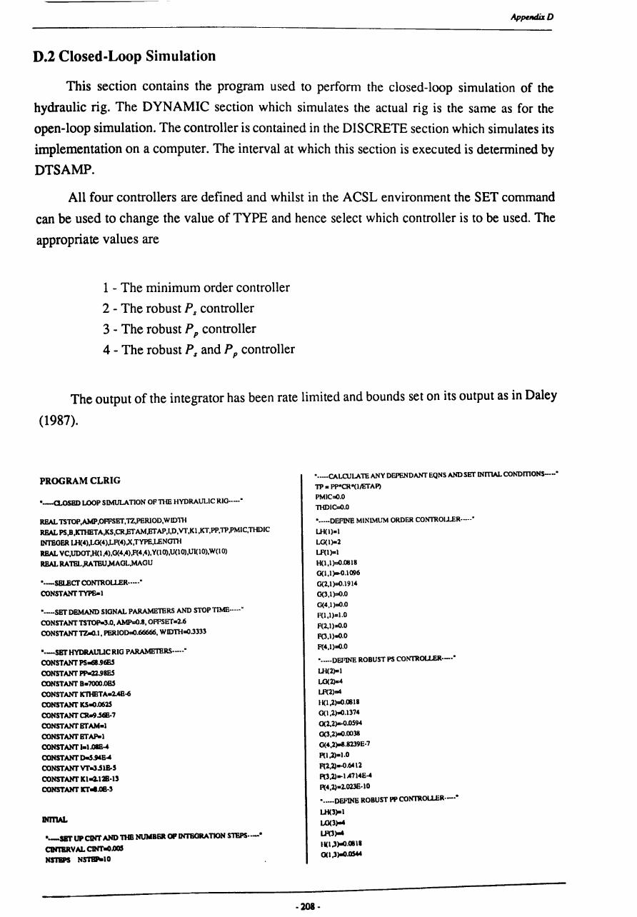
ApputdaD
D.2 Closed-Loop Simulation
This section contains the program used to perform the closed-loop simulation of the
hydraulic rig. The DYNAMIC section which simulates the actual rig is the same as for the
open-loop simulation. The controller is contained in the DISCRETE section which simulates its
implementation on a computer. The interval at which this section is executed is determined by
DTSAMP.
All four controllers are defined and whilst in the ACSL environment the SET command
can be used to change the value of TYPE and hence select which controller is to be used. The
appropriate values are
1 - The minimum order controller
2 - The robust Ps controller
3 - The robust P p controller
4 - The robust Ps and P p controller
The output of the integrator has been rate limited and bounds set on its output as in Daley
(1987).
PROGRAM CLRIG
·.-a.OSBD LOOP SIMULATION OF TIm HYDRAULIC RIG······
RBAL TSTOP,AMP,OFFSET,TZ,PERlOD,WIDTH RBAL PS,B,K1lIBTA,KS,CR.ET AM.ET AP,I,D,VT,KI,KT,PP,TP ,PMIC,THDIC
INTBGBR UI(4),LO(4),LF(4),x,TYPE,LENCTrn
RBAL VC,UDOT,H(I,4),0(4,4),F(4,4),Y(1O),U(10),U1(10),W(l0)
RBAL RA 11iL,RA 'Ilill,MAOL,MAOU
·.-SELBcr CONTROlLER······ CONSTANI'TYPB-I
·.-SET ORMAND SIGNAL PARAMETERS AND STOP TlMB·····
CONSTANI' TSTOM.O, AMP=O.8, OFFSET-2.6 CONSTANI' TZ-O.1, PBRIOD=O.66666, WIDTH=O.3333
·.-SET HYDRAULIC RIO PARAMETERS·_··
CONSTANI' pso61.9685
CONSTANI' PPw2l.98ES CONSTANI' B-7000.085 CONSTANI' K1lIBTA-2.4B-6 CONSTANI' KS.o.0625
CONSTANI' CR-9.56E-7
CONSTANI'ETAM-I
CONSTANI' ETAP-I CONSTANI' .. 1.0118-4
CONSTANI' o-.s.ME-4
CONSTANI'VT.J.51B-.5
CONSTANI' Kl0412B·lS CONSTANI' KT".OB·S
INITIAL
0-sBT UPCINT AND nIB NUMBBR OP DmKJRATION S1VS·-·
CIN18IlV AL CINT.o.005 NS'I1IPS N~lO
• ..... CALCULATE ANY DEPENDANT EQNS AND SET INITIAL CONDmONS--'
TP. PP·CR·(1JETAP) PMIC=O.O THDIC=O.O
• ••••• DEPINE MINIMUM ORDER CONTROLLER·_···
UI(1)-1
LG(1)-2 LF(I)-I
H(1,1 }=O.a1l8
0( 1,1)00-0.1 096
0(2,1 )=0.1914
0(3,1)=0.0
0(4,I}=O.0
F(1,I)=1.0 F(2,1)=O.0
F(3,I).o.O F(4,1)=O.0
• ••••• DEPINE ROBUST PS CONTROLLER·_··
Ul(2)a1
LO(2)c4
LF(2)""
11(1,2)=0.11118
0(1,2)=0.1374
0(2,2)c-O.OS94 0(3,2)=0.0038
0(4,2)008.8239E·7
F(I,2)-1.0
f(2,2)..o.6412
P{3,2)--IA714E-4
p{4,2)-1.023E·10
-lOB-
'.-0EFINIi ROBUST PP CONTRou..ER· ... ••
Ul(3)-1
1.0(3)004
LF(3)-'
11(1,3)000.1111'
0(I,3).().0S6I

0(2,3)000.0248
G(3,3)=O.oo26
0(4,3)-;5.9111 B-7
p(1,3)-1.0
P(2,3>-OA2S6
1'(3,3)-9.7342.8-S
p(4,3)-2.0230B-I0
··-DEFINE ROBUST PS AND PP CONTROL1.BR·_··
lJf(4)ool
LO(4,...
LP(4,...
H(1,4)ooO-'-18
0(1,4)=0.1321
0(2,4>-O.0S4
0(3,4)=0.0037
0(4,4)=8.6386B·7
P(1,4)=1
p(2,4)...o.6274
P(3,4)--1A397B-4
P(4,4).2.023B-I0
··-INrTlALISB SiGNALS·····
DOLl X '" 1,10
Y(X).O.O
U(X).O.O
U1(X).O.O
W(X).O.O
Ll .. CONTINUB
VC.O.O
···-SET INTEGRATOR OUTPUT BOUNDS······
RATBL=·O.5
RATBU.O.S
MAGL.·2.0
MAGU=2.0
BND S·OP INITIAL·
DYNAMIC
DBRIVATIVB
VlaAMP"PULSB(TZ,PBRIOD,WIDrn) + OFFSET
QV.KTIiETA "KS"VC"SQRT(PS·PMB)
PM.lNTBO((QV·CR "THD·K 1 "PMB)"2" B/VT),PMIC)
PMB=BOUND(·PS,PS,PM)
TM-PMOCR"ETAM
nIDaINTBG«TM·D"THD·TP)II,mDlC)
vOaKT"11ID
TBRMT(T.GB.TSTOP)
E."U S·OP DERIVATIVE·
DISCREll!
NJ"ERVAL DTSA.\fP=O.012
PR<Xr.DURAL (VC=VO,V I)
• .... ·MAINTAIN ARRAYS OP LAST TEN SA.'APUS-.·
DOL2X = 1,9
VeX) = Y(X+I)
W(X)=W(X+I)
U(X)=U(X+I)
UI(X) = UI(X+I)
L2 .. CONTINUE
• .... ·SA.\1PLE INPUT AND OlJl'PlIT ......
Y(10) =VO
W(10)=VI
•• .... CALCUlATB CONTROL SIGNAL-.. •
U(10) = 0.0
LENGTI-I = U-I(TYPE)
DO L3 X = I.LENGTH
U(10) = U(10) + 1I(X,TYPE)·W(1I·X)
L3 .. CONTINUE
LENGTII = I.O(TYPE)
DO L4 X = I ,LENGTH
U(lO) = U(lO)· G(X,1'YPE)·Y(lI·X)
L4 .. CONTINUE
LENGTII = IF(TYPE)
DO L5 X • 2,LENGTI1
U(10) .. U(lO)· F<X,TYPl,>"U(lI·X)
LS .. CONTlNUE
• .... ·CALaJlATB INTEGRAn;o CONTROL SIGNAL UI·_··
UI( 10) = U(10) + UI(9)
• .... ·RA·rn LlMrr CONTROL SiGNAL .... ••
UD01' .. U1(10)· UI(9)
IF(UDOT .LT.RATEL) UI(lO) = UI(9)+RATEL
IF (UDOT.GT.RATEU) UI(lO) = UI(9)+RATEU
•• .... MAGNl1lJDE BOlJJl.'OS ON CONTROL SiGNAL .... ••
IF (UI(lO).I.1' .MAGI.) UI(lO) = MAGI.
IF (UI(I O).GT.MAGU) UI(lO) .. MAGU
VC= UI(lO)
END S·OP PROCEDURAL·
EI\'O S·OP DISCRETE·
END S·OP DYNA.\tIC"
EI\'O S·OI' PROGRAM·
·209 .
Ap~D

GENERAL
RHS
w.r.t Z-1
a(t)
a(t-n)
E[a~t)]
Ap(Z-I)
III
diag[·]
I·D
I'D,
g'R p
1C(A)
[A].
A,
A,
M
dA
NOMENCLATURE AND SYMBOLS
Right hand side. With respect to.
Backward shift operator.
Discrete time signal.
Value of a(t) at the n'th previous sample.
Variance of a(t).
Pol ynomial in terms of the backward shift operator. Note that in chapter 2 polynomials are expressed
as Ap to make the notation more easy to follow.
Coefficients of the polynomial Aiz-I).
Estimate of Ap(Z-I).
Steady state value of Ap(Z-I).
Identity matrix of dimension n x n.
Zero matrix of dimension i x j .
Diagonal matrix.
Column vector.
Row vector.
General vector or matrix norm.
Frobenius norm.
P or Holder norm, where p = 1,2 or 00.
Condition number of the matrix A, defined as
1C{A) = IIAIIIIA -III The frrst x rows of the matrix A.
The frrst y columns of the matrix A.
Used in context to represent the sub-block of the matrix A.
Incremental change in A .
Differential of A .
Complex conjugate of A.
Real vector space of real n-dimensional vectors.
- 210-

Nomenclalure and Symbols
POLYNOMIAL SYSTEMS
wet)
u(t)
yet)
e(t)
a! d(t)
A,,(Z-l),
B,,{Z-l)
ttl
F,,(Z-l),
G,,{Z-l)
10th, ...
n~n,
nIl
nIl'
Demand signal.
Control input.
System output
White noise sequence.
Variance of e(/)
Disturbance term.
Open-loop system polynomials.
Coefficients of A,,(Z-l).
Coefficients of Bp(Z-l).
Orders of Ap(Z-l) and Bp(Z-l) respectively.
Colouring polynomial for the white noise sequence e(t).
Coefficients of Cp(Z-l).
Order of Cp{Z-l).
Time delay.
Controller polynomials.
Coefficients of Fp(Z-l).
Coefficients of G,(Z-l).
Orders of Fp(Z-l) and Gp(Z-l) respectively.
Precompensator polynomial.
Coefficients of Hp(Z-l).
Order of H,,(Z-l).
Precompensator term selected for zero steady state error.
Order of H/{Z-l).
Polynomial used to specify the desired closed-loop pole positions.
Coefficients of T,,(Z-l).
Order of T,,(Z-l).
- 211 -

Nomenclalure and Symbols
Solution of the Diophantine Equation by Polynomial Methods
GCD
coro
Greatest common divisor.
QeD of Ap(z-l) and Bp(Z-l).
Solution to the diophantine equation.
Arbitrary polynomial in general solution.
Result of dividing Cp(z-l)Tp(Z-l) by gp and must be polynomial for a solution to exist.
Pair of coprime polynomials which satisfy A P + B Q = g p p p p po
Pair of coprime polynomials which satisfy A R + B S = 0 p p p p .
Quotient polynomial.
Remainder polynomial.
Solution of the Diophantine Equation by Matrix Methods
N,
Sylvester matrix.
Vector of the coefficients of Fp(Z-I) and Gp(Z-I).
Vector of the coefficients of Cp{z-I)Tp(z-I).
Upper bound on the relative perturbation, II L1!1I III ~n . Number of columns of A6 •
Number of rows of A6 •
Number of unknowns (the number of Fiz-1) and Gp{Z-I) coefficients).
Number of equations represented by A~ = /2...
STATE SPACE SYSTEMS
n
m
r
k
u(k)
y(k)
!.(k)
l.(k)
:!'<k)
A,BtC
p
Number of states.
Number of inputs.
Number of outputs.
Discrete time sequence.
Input signal equivalent to the input for the polynomial system.
Output signal equivalent to the output for the polynomial system.
Multivariable input signal (with augmented dynamic compensator).
Multivariable output signal (with augmented dynamic compensator).
Slate vector.
Open-loop system matrices
Closed-loop system matrix.
Order of the dynamic compensator.
- 212-

K,
v L F
w
G
Output feedback controller gain matrix.
State feedback controller gain matrix.
The i'th closed-loop eigenvalue.
Set of closed-loop eigenvalues.
The i'th right eigenvector.
Matrix of right eigenvectors.
The associated i'th right free parameter vector.
Matrix of right free parameter vectors.
The i'th left eigenrow.
Matrix of left eigenrows.
The associated i'th left free parameter vector.
Matrix of left free parameter vectors.
Nomenclature and Symbols
The Parametric Method of Fahmy and O'Reilly
s
B
C
K
Defines the split for the multistage design.
Input reduction matrix.
Output reduction matrix.
General Output feedback controller gain matrix obtained by either the first or second stage.
Controller gain matrix obtained by the first stage.
Controller gain matrix obtained by the second stage.
Output feedback controller gain matrix obtained after the application of either an input or
output reduction matrix.
The Parametric Method of Daley
r
=n-r.
The first r columns of the matrix F.
The r + 1 to n columns of the matrix F.
Sub-blocks of the matrix V.
i'th column of Vn'
Vector consisting of all the vectors in Fl'
r must lie in the null space of this matrix.
For i = r + 1 -+ n, specifies the set of matrices whose null spaces the F 2 vectors must lie in.
- 213-

COST FUNCTIONS
u
P,
Q,
1i1
Number of error terms.
Structural information on the errors in A.
Structural information on the errors in B.
Unknown magnitude of the t'th error term.
Eigenvalue differential cost function.
Eigenstructure differential cost function.
Transient response differential cost function.
Conditioning cost function.
Weights used in the eigenvalue differential cost function.
Weights used in the eigenstructure differential cost function.
Weights used in the transient response differential cost function.
Weight used when combining terms in a cost function.
IMPLEMENTATION AND APPLICATION OF THE METHOD
SVD Singular value decomposition.
A, Real matrix or real part of a complex matrix.
Ai Imaginary part of a complex matrix.
AI: Used in context to denote a complex matrix.
Nt Number of free parameters.
N,. Number of residuals.
XT Vector specifying the initial values for the free parameters.
WT Vector specifying the values of the weights
J",iI Original value of the cost function.
J., Final value of the cost function.
HYDRAULIC RIG
Qv Flow rate through the spool valve.
X, Spool valve displacement.
P, Supply pressure.
PIA Pressure differential across the motor.
K. Valve flow coefficient
e Shaft position.
er Motor displacement.
·214·
Nomenclature and Symbols

v,
T".
1l".
1
D
K.
K,
u
y
VN
FPE
N
p
8,
£(1,8,)
Total trapped volume.
Oil bulk modulus.
Leakage coefficient
Motor torque.
Efficiency of the motor.
Total inertia.
Viscous friction coefficient.
Pressure differential across the pump.
Efficiency of the pump.
Pure gain term for the servo and torque motor.
Tachometer constant.
Input voltage.
Output voltage.
Loss function.
Akaike's final prediction error.
Number of data points.
Number of parameters in the model.
Parameter vector.
Prediction error.
Nomenclalure and Symbols