Robust Portfolio Optimization Usinga Simple Factor Model

Chris Bemis, Xueying Hu, Weihua Lin, Somayeh Moazeni,

Li Wang, Ting Wang, Jingyan Zhang

Abstract

In this paper we examine the performance of a traditional mean-variance optimized portfolio, wherethe objective function is the Sharpe ratio. We show results of constructing such portfolios using globalindex data, and provide a test for robustness of input parameters. We continue by formulating a robustcounterpart based on a linear factor model presented here. Using a dynamic universe of stocks, theresults for this robust portfolio are contrasted with a naive, evenly weighted portfolio as well as withtwo traditional Sharpe optimized portfolios. We find compelling evidence that the robust formulationprovides significant risk protection as well as the ability to provide risk adjusted returns superior to thetraditional method. We also find that the naive portfolio we present outperforms the traditional Sharpeportfolios in terms of many summary metrics.

1 Introduction

We begin by examining the performance of a traditional Sharpe ratio optimization problem using globalindexes in Section 2. Here we establish the quadratic programming problem of interest to us and exhibit thenonstationarity of the input parameters. We proceed in Section 3 to add additional constraints to the originalproblem to mimic realistic portfolio positions and strategies. The performance of a monthly rebalancedoptimal portfolio based on these constraints is shown. We also perform a simple test for robustness, noticingthat the optimal weights produced in the mean-variance optimal setting are sensitive to initial conditions.This leads us to a variation of the work of Goldfarb and Iyengar in Section 4. There we also provide aformulation similar to their work using an ellipsoidal uncertainty set for the vector of mean returns.

We develop a linear factor model motivated in part by the work of Fama and French. We conduct cross-sectional regressions to fit the regression parameters and note a term structure for these factor returns. Thisdeviates from the regression procedure in Goldfarb and Iyengar. We therefore develop our own variationof uncertainty in input parameters in Section 4.4. For our asset universe, we consider stocks determineddynamically by a lower bound of $10 billion for market capitalization. We avoid survivorship bias as muchas possible by selecting all stocks that have traded at least once over the history we are interested in.

The performance of the linear model ex-post is evaluated using a lagged lter. We observe summaryportfolio statistics superior to those obtained in a standard mean-variance optimized portfolio constructedin 5. There we also show the results of the robust counterpart. These results provide compelling evidencethat, in contrast to the nominal problem, the robust problem in fact delivers a portfolio with intendedcharacteristics; e.g., higher Sharpe with more attractive loss profiles.

1

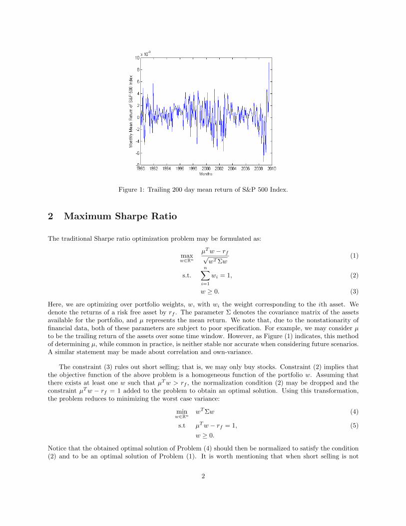
Figure 1: Trailing 200 day mean return of S&P 500 Index.

2 Maximum Sharpe Ratio

The traditional Sharpe ratio optimization problem may be formulated as:

maxw∈ℝn

�Tw − rf√wTΣw

(1)

s.t.

n∑i=1

wi = 1, (2)

w ≥ 0. (3)

Here, we are optimizing over portfolio weights, w, with wi the weight corresponding to the ith asset. Wedenote the returns of a risk free asset by rf . The parameter Σ denotes the covariance matrix of the assetsavailable for the portfolio, and � represents the mean return. We note that, due to the nonstationarity offinancial data, both of these parameters are subject to poor specification. For example, we may consider �to be the trailing return of the assets over some time window. However, as Figure (1) indicates, this methodof determining �, while common in practice, is neither stable nor accurate when considering future scenarios.A similar statement may be made about correlation and own-variance.

The constraint (3) rules out short selling; that is, we may only buy stocks. Constraint (2) implies thatthe objective function of the above problem is a homogeneous function of the portfolio w. Assuming thatthere exists at least one w such that �Tw > rf , the normalization condition (2) may be dropped and theconstraint �Tw − rf = 1 added to the problem to obtain an optimal solution. Using this transformation,the problem reduces to minimizing the worst case variance:

minw∈ℝn

wTΣw (4)

s.t �Tw − rf = 1, (5)

w ≥ 0.

Notice that the obtained optimal solution of Problem (4) should then be normalized to satisfy the condition(2) and to be an optimal solution of Problem (1). It is worth mentioning that when short selling is not

2

allowed, and ri < 0 for all i = 1, 2, ..., n, an optimal solution of Problem (4) is not necessarily an optimalsolution of Problem (1), and the transformation does not remain valid. Indeed, negative Sharpe ratio isconsidered ambiguous and is not typically considered (for a through discussion the reader is referred to[7]). To alleviate negative Sharpe ratios, one may permit short selling when maximizing the Sharpe ratio.Alternatively, one may use other objectives, such as minimizing variance of the return, or heuristic algorithms[6].

Assuming that rf ≥ −1, the constraint (5) may be relaxed by �Tw− rf ≥ 1, since the relaxed constraintwill always be tight at an optimal solution. Therefore, we are left to solve the following problem:

minw∈ℝn

wTΣw (6)

s.t �Tw − rf ≥ 1, (7)

w ≥ 0.

When the covariance matrix Σ is positive definite, Problem (6) is a (strictly) convex quadratic program-ming problem and has a unique solution.

We also consider additional problems by varying the constraints found in Problem (1). For example,investors typically prefer not to invest all of their money in one stock. This is a result of both theory andpractice: we see that portfolio risk may be mitigated if true diversification is possible (e.g., in the case wherewe find assets that retain low correlation even in so-called fear environments), and performance of, say, aneven weighted portfolio may often times have more desirable characteristics than an otherwise unconstrainedMVO optimal portfolio [1]. Therefore, to obtain a more diversified portfolio we also consider constrainingmaximum position sizes below, e.g., Problems (9) and (10). In the next section, we describe the portfolioswe consider in this preliminary analysis.

In light of the potential for poor specification of the input parameters noted above, we also examine therobustness of the algorithm to perturbations in �.

3 Analysis of Traditional Sharpe Optimization

To obtain insight about the effectiveness of various portfolios constructed using the methodology describedabove, we use a universe of five assets made up of global indexes. For this fixed set of assets, we considerfour portfolios, described below.

We use daily close prices for five stock indexes from January 1990 to August 2009 to estimate � and Σas above. These indexes include the S&P 500 in the United States (SPX), the FTSE 100 (UKX) in London,the French CAC 40, the German DAX, and the Hang Seng (HSI) in Hong Kong. Since each country hasdifferent holidays and non-trading days, we face an issue of incomplete return data; if a particular index’srecord is incomplete in a given day, we could either interpolate this return or simply ignore it. Interpolatingthe missing return data maintains the sample size; however, it creates bias for our estimation, and couldchange the correlation between the indexes. Ignoring or deleting an incomplete record, on the other hand,reduces the sample size. In our case, only one to two days out of about twenty trading days were deletedin such months. Taking this into consideration, we choose to eliminate days for which not all indexes havedata. We nevertheless ran the tests both, and the results for portfolios constructed where incomplete datawas omitted outperformed those portfolios constructed using the interpolation techniques we employed.

3

Once � and Σ are determined, we determine optimal weights wi monthly throughout our historical periodby solving the maximum Sharpe ratio problem under various constraints:Portfolio (P1): Short selling is not allowed and rf = 0:

maxw

�Tw√wTΣw

s.t

n∑i=1

wi = 1, w ≥ 0. (8)

Portfolio (P2): Maximum investment on each asset is bounded and a cash account earning LIBOR isintroduced so that rf ∕= 0:

maxw

�Tw − rf√wTΣw

s.t

n∑i=1

wi = 1, 0 ≤ w ≤ 0.5. (9)

Portfolio (P3): Short selling is allowed and rf = 0:

maxw

�Tw√wTΣw

s.t

n∑i=1

(wi)+ = 1,

n∑i=1

(wi)− = −1, ∣wi∣ ≤ 0.5, i = 1, 2, ..., n. (10)

To obtain the optimal solution of Problem (10), we solve the following problem:

min vT

(Σ −Σ

−Σ Σ

)v, s.t (�, �)T v ≥ 1, ∣vi∣ ≤ 0.5,

5∑i=1

vi = 1,

10∑i=6

vi = −1,

or equivalently

min vT(

Σ −Σ

−Σ Σ

)v, s.t (�, �)T v ≥ 1, vi ≤ 0.5

5∑i=1

vi, i = 1, ..., 5, vi ≤ 0.5

10∑i=6

vi, i = 6, ..., 10. (11)

Then the optimal solution of Problem (10) is

w∗ =1∑5i=1 v

∗i

⎛⎜⎜⎝v∗1...

v∗5

⎞⎟⎟⎠+1∑10i=6 v

∗i

⎛⎜⎜⎝v∗6...

v∗10

⎞⎟⎟⎠ ,

where v∗ is the optimal solution of Problem (11). We used CVX: Matlab Software for Disciplined ConvexProgramming to solve this problem.

An optimal solution of Problem (10) may be found by solving the following solution:

minw wT Σw, (12)

�Tw ≥ 1n∑

i=1

wi = 0,

(wi)+ ≤ 0.5

n∑i=1

(wi)+, i = 1, 2, ..., n,

(wi)− ≤ −0.5

n∑i=1

(wi)−, i = 1, 2, ..., n,

(13)

This is because every optimal solution of Problem (10) is an optimal solution of Problem (12). Conversely,

assume that w∗ is an optimal solution of Problem (12). Now wi =w∗

i∑(w∗

i )+if w∗i ≥ 0 and wi =

w∗i

∣∑

(w∗i )−∣

if

w∗i ≤ 0 is an optimal solution of Problem (10). Here we included the constraint∑ni=1 wi = 0 to guarantee

that the total weights for shorts equal the total weights for long trades.

4

Proposition 3.1. The optimal solution of the above problem can be obtained by solving the following prob-lem:

minw wT Σw, (14)

�Tw ≥ 1n∑

i=1

wi = 0,

wi ≤ ti ≤ 0.5

n∑i=1

ti, i = 1, 2, ..., n,

−0.5

n∑i=1

si ≤ si ≤ wi, i = 1, 2, ..., n,

si + ti = wi, i = 1, 2, ..., n, (15)

s2i + t2i = w2i , i = 1, 2, ..., n, (16)

si ≤ 0, ti ≥ 0, i = 1, 2, ..., n.

Proof. Let w∗i be a solution of Problem (12). Then t∗i = max{0, wi} and s∗i = min{0, wi} satisfies theproblem. So (w∗i , t

∗i , s∗i ) is an optimal solution of Problem (14). Now assume (w∗i , t

∗i , s∗i ) is an optimal

solution of Problem (14). Then constraints (15) and (16) implies that s∗i t∗i = 0. Since si ≤ 0, ti ≥ 0 and

si + ti = wi we must have t∗i = max{0, wi} and s∗i = min{0, wi}.

3.1 Performance with Select Index Data

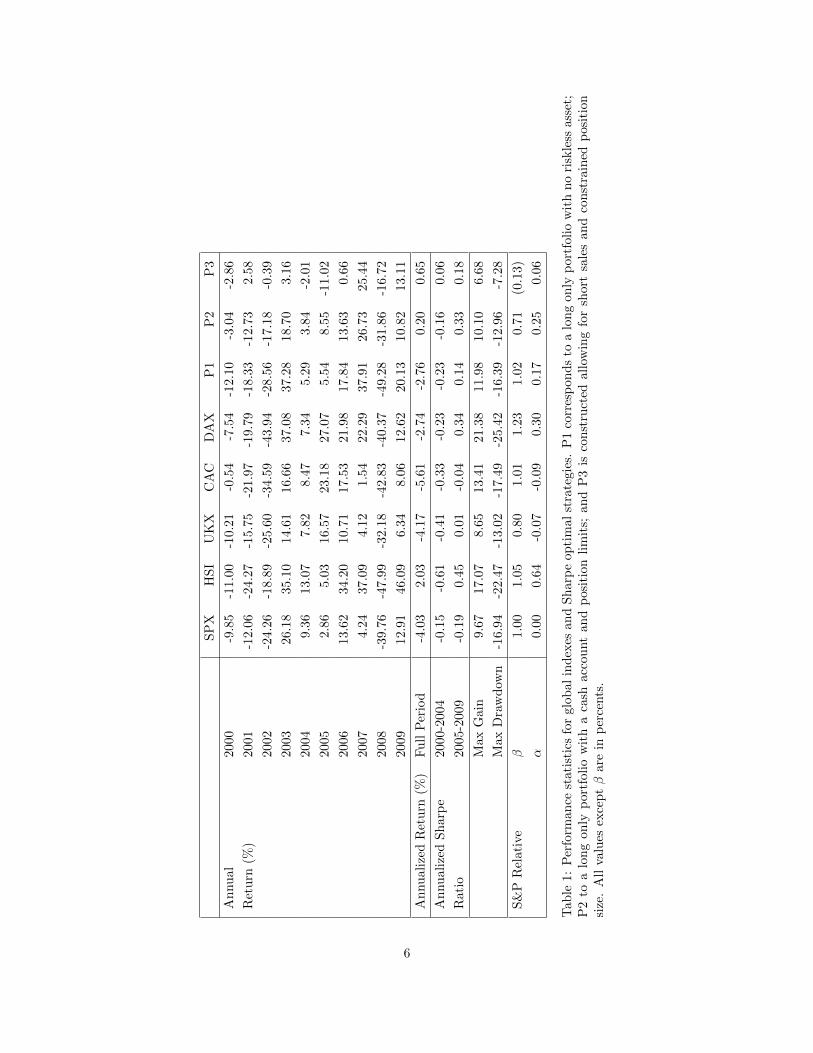
The comparison of the performance of the above strategies is shown in Table (1). These data are obtainedusing a monthly rebalancing strategy. That is, optimal weights w are computed at the end of every month,and these weights are used to determine performance over the next calendar month. In the first five columns,the performance of the constituent indexes are shown. The last three columns correspond to the investmentbased on strategies (P1)-(P3) as previously described.

From the table, we can see that the the performance of portfolio P1 is oftentimes closely related to thatof Hang Seng. This is a result of the lack of a maximum exposure constraint. In many months, most or all ofthe weight was put into the HSI for this portfolio. In particular, we note that the optimal weights essentiallyoffer a trend tracking strategy. Also, since only long positions are allowed in this case, a dramatic drop isinventible during 2008. This is relieved to some extent in portfolio P2.

Recall that when computing the portfolio P2, we required that no weight constituted more than 50% ofthe total portfolio exposure. This was introduced to guarantee some measure of diversity. This condition,along with the availability of a risk free asset produces a portfolio where some risk has been mitigated, andmarket exposure, i.e., �, has been reduced relative to the unconstrained portfolio.

In portfolio P3, we allow short selling. Theoretically, short positions allow for gains in a portfolio evenwhen the market at large may be dropping. An example of this type of protection is witnessed in 2001.However, during other down years, P3 does not generate positive returns. It does afford some protection,though. Notice that while we don’t see gains in 2008 for this portfolio, P3 does have the minimum monthlydrawdown among all the portfolios considered; most of which occurred during this dramatic year.

Overall, P1 and P2 do not show significant advantage over the indexes. However, both P1 and P2produce a positive � relative to the S&P, albeit with significant market exposure. The portfolio constructedusing the constraints found in P3, yields a relatively low �, and maintains a (smaller) positive �. This

5

SP

XH

SI

UK

XC

AC

DA

XP

1P

2P

3

An

nu

al20

00-9

.85

-11.0

0-1

0.2

1-0

.54

-7.5

4-1

2.1

0-3

.04

-2.8

6

Ret

urn

(%)

2001

-12.0

6-2

4.2

7-1

5.7

5-2

1.9

7-1

9.7

9-1

8.3

3-1

2.7

32.5

8

2002

-24.2

6-1

8.8

9-2

5.6

0-3

4.5

9-4

3.9

4-2

8.5

6-1

7.1

8-0

.39

2003

26.1

835.1

014.6

116.6

637.0

837.2

818.7

03.1

6

2004

9.3

613.0

77.8

28.4

77.3

45.2

93.8

4-2

.01

2005

2.8

65.0

316.5

723.1

827.0

75.5

48.5

5-1

1.0

2

2006

13.6

234.2

010.7

117.5

321.9

817.8

413.6

30.6

6

2007

4.2

437.0

94.1

21.5

422.2

937.9

126.7

325.4

4

2008

-39.7

6-4

7.9

9-3

2.1

8-4

2.8

3-4

0.3

7-4

9.2

8-3

1.8

6-1

6.7

2

2009

12.9

146.0

96.3

48.0

612.6

220.1

310.8

213.1

1

An

nu

aliz

edR

eturn

(%)

Fu

llP

erio

d-4

.03

2.0

3-4

.17

-5.6

1-2

.74

-2.7

60.2

00.6

5

An

nu

aliz

edS

har

pe

2000

-200

4-0

.15

-0.6

1-0

.41

-0.3

3-0

.23

-0.2

3-0

.16

0.0

6

Rat

io20

05-2

009

-0.1

90.4

50.0

1-0

.04

0.3

40.1

40.3

30.1

8

Max

Gai

n9.6

717.0

78.6

513.4

121.3

811.9

810.1

06.6

8

Max

Dra

wd

own

-16.9

4-2

2.4

7-1

3.0

2-1

7.4

9-2

5.4

2-1

6.3

9-1

2.9

6-7

.28

S&

PR

elat

ive

�1.0

01.0

50.8

01.0

11.2

31.0

20.7

1(0

.13)

�0.0

00.6

4-0

.07

-0.0

90.3

00.1

70.2

50.0

6

Tab

le1:

Per

form

ance

stat

isti

csfo

rgl

obal

ind

exes

an

dS

harp

eop

tim

al

stra

tegie

s.P

1co

rres

pon

ds

toa

lon

gon

lyp

ort

foli

ow

ith

no

risk

less

ass

et;

P2

toa

lon

gon

lyp

ortf

olio

wit

ha

cash

acco

unt

an

dp

osi

tion

lim

its;

an

dP

3is

con

stru

cted

all

owin

gfo

rsh

ort

sale

san

dco

nst

rain

edp

osi

tion

size

.A

llva

lues

exce

pt�

are

inp

erce

nts

.

6

portfolio, along with P2, also has a positive annualized return over the period under investigation. Amongthe indexes, only the Hang Seng shows a positive return over this time.

3.2 Sensitivity Analysis

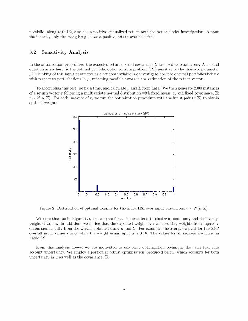
In the optimization procedures, the expected returns � and covariance Σ are used as parameters. A naturalquestion arises here: is the optimal portfolio obtained from problem (P1) sensitive to the choice of parameter�? Thinking of this input parameter as a random variable, we investigate how the optimal portfolios behavewith respect to perturbations in �, reflecting possible errors in the estimation of the return vector.

To accomplish this test, we fix a time, and calculate � and Σ from data. We then generate 2000 instancesof a return vector r following a multivariate normal distribution with fixed mean, �, and fixed covariance, Σ;r ∼ N(�,Σ). For each instance of r, we run the optimization procedure with the input pair (r,Σ) to obtainoptimal weights.

Figure 2: Distribution of optimal weights for the index HSI over input parameters r ∼ N(�,Σ).

We note that, as in Figure (2), the weights for all indexes tend to cluster at zero, one, and the evenly-weighted values. In addition, we notice that the expected weight over all resulting weights from inputs, rdiffers significantly from the weight obtained using � and Σ. For example, the average weight for the S&Pover all input values r is 0, while the weight using input � is 0.16. The values for all indexes are found inTable (2)

From this analysis above, we are motivated to use some optimization technique that can take intoaccount uncertainty. We employ a particular robust optimization, produced below, which accounts for bothuncertainty in � as well as the covariance, Σ.

7

Index Average of Weights over r ∼ N(�,Σ) Weights Using (�,Σ)

SPX 0.0000 0.1593

HSI 0.0849 0.1857

UKX 0.6260 0.2979

CAC 0.1309 0.1531

DAX 0.1582 0.2040

Table 2: Comparison of average of optimal weights for the indexes over input parameters r ∼ N(�,Σ) withthe weight obtained using � and Σ.

4 Robust Maximum Sharpe Ratio Problem and a Linear FactorModel

We follow Goldfarb and Iyengar’s problem formulation for a robust Sharpe problem [3] to introduce modeluncertainty into our optimization procedure. We construct both a linear factor model based in part on thework of Fama and French [2] as well as a new uncertainty set for the vector of expected returns. In addition,we adapt a cross sectional regression methodology to the structure found in [3]. While our adaptation straysfrom the parsimonious uncertainty sets of Goldfarb and Iyengar, our implementation retains key elementsof their method wherever possible.

4.1 Overview of Goldfarb and Iyengar Model and a Variation in UncertaintySets

Goldfarb and IyengarHere [3] assume that the return vector follows a linear factor model as in (24):

r = �+ V T f + �, (17)

where � is the expected return vector, f ∼ N (0, F ) ∈ ℝm is the returns of the factors that are assumed todrive market returns, V ∈ ℝm×n is the factor loading matrix of the n assets and � ∼ N (0,D) ∈ ℝn is themodel residual. Also, we suppose that the residual return vector, �, is independent of the vector of factorreturns f , the covariance matrix F ≻ 0 and the covariance matrix D = diag(d) ર 0. Thus, the vector ofasset returns r ∼ N (�, V TFV + D).

Similar to [3], we assume that the mean return �, factor loading V , and error covariance D are subjectto uncertainty. The uncertainty set Sd for the matrix D is given by

Sd = {D : D = diag(d), di ∈ [di, di], i = 1, . . . , n} (18)

where the individual diagonal elements di of D are assumed to lie in an interval [di, di]

We assume that the columns of the matrix V belong to the elliptical uncertainty set Sv given by

Sv = {V : V = V0 +W, ∥Wi∥g ≤ �i, i = 1, ..., n} , (19)

where Wi is the i-th column of W and ∥w∥g =√wTGw denotes the elliptic norm of w with respect to a

symmetric, positive definite matrix G. In [3], an interval uncertainty set is used to explain the uncertaintyin the mean return:

{� : � = �0 + �, ∣�i∣ ≤ i, i = 1, ..., n} , (20)

8

We introduce here the uncertainty set, S̃m defined by

S̃m =

⎧⎨⎩� : � = �0 −k∑j=1

uj�(j), uTu ≤ 1

⎫⎬⎭ . (21)

This set is considered so as to provide a method to retain the joint distribution of the returns, r, whenallowing uncertainty in our expectation. Specifically, we choose �(j) above to be the column vectors of thecovariance matrix of returns being modeled, and �0 to be the expected return. We note that we do notretain the regression-focused derivation for the uncertainty in � as in [3].

Using the uncertainty sets Sv, S̃m and Sd, the robust maximum Sharpe ratio problem is given by

max{w:w≥0,1Tw=1}

minV ∈Sv,�∈S̃m,D∈Sd

�Tw − rf√wTΣw

.

We will assume that the optimal value of this max-min problem is strictly positive, i.e., that there is at leastone asset with worst case return greater than rf . The robust Sharpe ratio reduces to minimizing the worstcase variance:

minw

maxV ∈Sv

wTV TFV w + wT D̄w,

min�∈Sm

(�− rf1)Tw ≥ 1. (22)

The constraint min�∈Sm(�− rf1)Tw equals

min�∈Sm

(�− rf1)Tw = min�∈Sm

⎛⎝�0 −k∑j=1

uj�(j) − rf1

⎞⎠T

w

= (�0 − rf1)Tw − max

{u:∥u∥2≤1}

k∑j=1

uj(�(j))Tw

= (�0 − rf1)Tw −

√√√⎷ k∑j=1

((�(j))Tw)2 = (�0 − rf1)Tw − ∥Mw∥2,

where the last inequality comes from the definition of dual norms. Thus constraint (25) equals to thefollowing constraint:

(�0 − rf1)Tw ≥ 1 + ∥Mw∥2,

where the jth row of the matrix M is (�(j))T . Using the discussion in [3], the robust counterpart problemis reduced to the following second order cone programming problem:

min�,�,t,v,�,w

v + � (23)

s.t ∥[2D̄ 12w; 1− �]∥ ≤ 1 + �,

∥Mw∥2 ≤ (�0 − rf1)Tw − 1,

(�Tw; v;w) ∈ ℋ(V0, F,G).

where ℋ(V0, F,G) is defined as below:

9

Definition 4.1. Given V0 ∈ ℝm×n and F,G ∈ ℝm×m ≻ 0, define ℋ(V0, F,G) to be the set of all vectors(r, v, w) ∈ ℝ× ℝ× ℝn satisfying the following: there exists �, � and t ∈ ℝm that satisfy

�, �, t ≥ 0,

� + 1T t ≤ v,

� ≤ 1

�max(H),

∥[2r;� − � ]∥ ≤ � + �,

∥[2(QTH12G

12V0w)i; 1− ��i − ti]∥ ≤ 1− ��i + ti, i = 1, ...,m

where QΛQT is the spectral decomposition of H = G−12FG−

12 , Λ = diag(�i).

Notice that in the derivation of the robust counterpart problem, no assumption is made about nonneg-ativity of the weights. Further, while the uncertainty sets of Goldfarb and Iyengar are intimately relatedto the model (24), we note that after the sets Sv, S̃m and Sd are determined, the robust problem is notdependent on (24).

Clearly, to construct such robust Sharpe portfolios, we are required to model returns linearly based onfactors f . Below we construct a linear factor model to implement the program just outlined, with someadjustments.

4.2 Linear Factor Model and Stock Universe

Fama and French in [2] model a cross-section of stock returns based on loadings according to three factorsthat mimic market exposure, size and value using market beta, market capitalization, and book to price,respectively. Motivated by their work, we employ a similar factor model. In our model, we use asset specificfactors:

∙ Market value: the total value of all common shares currently outstanding.

∙ Book-to-price: the ratio of the tangible book value to the market value.

∙ Debt-to-equity: the ratio of the total long term debt to market value.

∙ Asset growth: the year over year growth in assets as a percent.

∙ One month trailing return: the return over the most recently completed month.

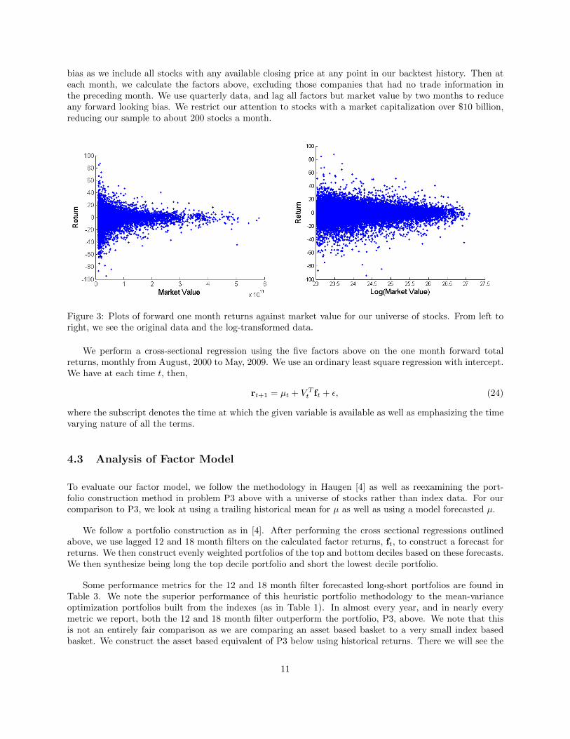
We calculate factor values monthly based on a universe of stocks described below. We normalize all vari-ables based on the factor specific cross-sectional mean and variance. Additionally, prior to the normalizationof market value, we employ a log transformation. The plots in Figure (3) show the scatter plot of monthlyreturns against market value, before and after a log transformation, respectively. These plot confirms thephenomenon that as the size of a company increases, the variance of returns decreases. We see that takingthe log not only greatly reduces the scale of the factor, but also stabilizes the conditional variance. In ad-dition to normalization and transformation, we replace unreported factor values with the factor populationmean.

Our universe of stocks is constructed monthly from a Compustat database at the end of each month fromAugust 2000 to May, 2009. To the best of our ability, our implementation does not suffer from survivorship

10

bias as we include all stocks with any available closing price at any point in our backtest history. Then ateach month, we calculate the factors above, excluding those companies that had no trade information inthe preceding month. We use quarterly data, and lag all factors but market value by two months to reduceany forward looking bias. We restrict our attention to stocks with a market capitalization over $10 billion,reducing our sample to about 200 stocks a month.

Figure 3: Plots of forward one month returns against market value for our universe of stocks. From left toright, we see the original data and the log-transformed data.

We perform a cross-sectional regression using the five factors above on the one month forward totalreturns, monthly from August, 2000 to May, 2009. We use an ordinary least square regression with intercept.We have at each time t, then,

rt+1 = �t + V Tt ft + �, (24)

where the subscript denotes the time at which the given variable is available as well as emphasizing the timevarying nature of all the terms.

4.3 Analysis of Factor Model

To evaluate our factor model, we follow the methodology in Haugen [4] as well as reexamining the port-folio construction method in problem P3 above with a universe of stocks rather than index data. For ourcomparison to P3, we look at using a trailing historical mean for � as well as using a model forecasted �.

We follow a portfolio construction as in [4]. After performing the cross sectional regressions outlinedabove, we use lagged 12 and 18 month filters on the calculated factor returns, ft, to construct a forecast forreturns. We then construct evenly weighted portfolios of the top and bottom deciles based on these forecasts.We then synthesize being long the top decile portfolio and short the lowest decile portfolio.

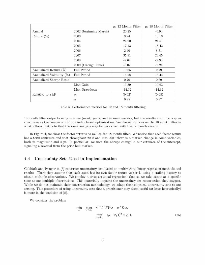
Some performance metrics for the 12 and 18 month filter forecasted long-short portfolios are found inTable 3. We note the superior performance of this heuristic portfolio methodology to the mean-varianceoptimization portfolios built from the indexes (as in Table 1). In almost every year, and in nearly everymetric we report, both the 12 and 18 month filter outperform the portfolio, P3, above. We note that thisis not an entirely fair comparison as we are comparing an asset based basket to a very small index basedbasket. We construct the asset based equivalent of P3 below using historical returns. There we will see the

11

�: 12 Month Filter �: 18 Month Filter

Annual 2002 (beginning March) 20.25 -0.94

Return (%) 2003 3.24 13.13

2004 24.90 24.51

2005 17.13 18.43

2006 2.40 8.71

2007 35.91 24.65

2008 -9.62 -9.36

2009 (through June) -8.07 -2.24

Annualized Return (%) Full Period 10.65 9.79

Annualized Volatility (%) Full Period 16.28 15.44

Annualized Sharpe Ratio 0.70 0.69

Max Gain 13.39 10.63

Max Drawdown -14.32 -14.62

Relative to S&P � (0.02) (0.08)

� 0.95 0.87

Table 3: Performance metrics for 12 and 18 month filtering.

18 month filter outperforming in some (most) years, and in some metrics, but the results are in no way asconclusive as the comparison to the index based optimization. We choose to focus on the 18 month filter inwhat follows, but note that the same analysis may be performed with the 12 month version.

In Figure 4, we show the factor returns as well as the 18 month filter. We notice that each factor returnhas a term structure and that throughout 2008 and into 2009 there is a marked change in some variables,both in magnitude and sign. In particular, we note the abrupt change in our estimate of the intercept,signaling a reversal from the prior bull market.

4.4 Uncertainty Sets Used in Implementation

Goldfarb and Iyengar in [3] construct uncertainty sets based on multivariate linear regression methods andresults. There they assume that each asset has its own factor return vector f , using a trailing history toobtain multiple observations. We employ a cross sectional regression; that is, we take assets at a specifictime as our multiple observations. This materially impacts the uncertainty set construction they suggest.While we do not maintain their construction methodology, we adapt their elliptical uncertainty sets to oursetting. This procedure of using uncertainty sets that a practitioner may deem useful (at least heuristically)is more in the tradition of [8].

We consider the problem

minw

maxV ∈Sv

wTV TFV w + wT D̄w,

min�∈Sm

(�− rf1)Tw ≥ 1, (25)

12

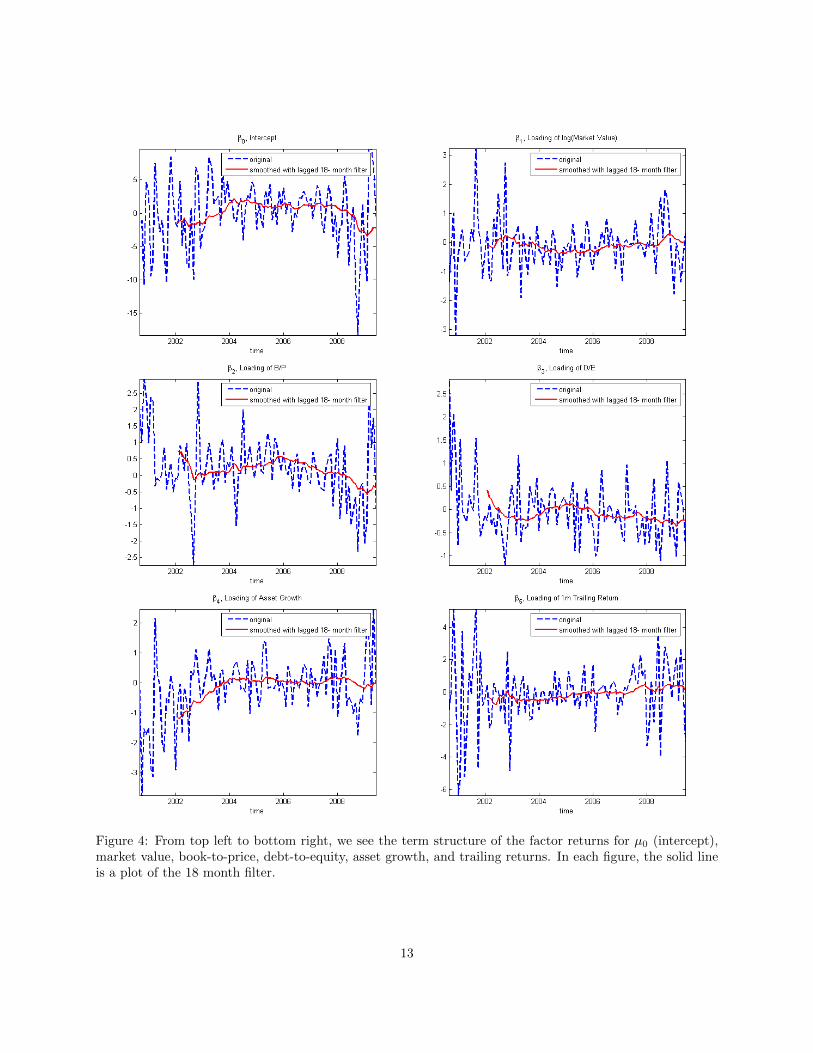
Figure 4: From top left to bottom right, we see the term structure of the factor returns for �0 (intercept),market value, book-to-price, debt-to-equity, asset growth, and trailing returns. In each figure, the solid lineis a plot of the 18 month filter.

13

where

Sd = {D : D = diag(d), di ∈ [di, di], i = 1, . . . , n},

Sv = {V : V = V0 +W, ∥Wi∥g ≤ �i, i = 1, ..., n} ,

Sm = {� : � = �0 + �, ∣�i∣ ≤ i, i = 1, ..., n} .

Recall that this was the problem derived from

maxw∈W

minV ∈Sv,�∈Sm,D∈Sd

�Tw − rf√wTΣw

,

where the return vector is assumed to follow (24), and W is some constraint set on the weights w. Further,this problem may be written as a second order cone program as in (23), with slight modification.

We are left then to determine the bounds di, �i , and i , for i = 1, . . . , n, and to define the ellipticalnorm in the set definition for Sv. While our sets are not entirely motivated by regression uncertainty, wemake only slight modifications. The interested reader may see [3] for the initial development of what follows.

We begin by choosing to use 18 months of trailing factor returns, ft, for what follows. Since our modelingis cross-sectional, we look temporally for the variance of factor returns, F . We define the matrix B as

B = [ft−p ⋅ ⋅ ⋅ ft−2 ft−1]. (26)

with p = 18. For ease of notation, we include the intercept term from above in fcdot here and for theremainder. This gives the maximum likelihood estimate for the covariance of factor returns:

F =1

p− 1⋅(B ⋅BT − (B ⋅ 1) ⋅ (B ⋅ 1)T

), (27)

with 1 a vector of ones with p rows. We define G as G = (p− 1) ⋅F , and the elliptical norm ∥⋅∥g is given by

∥x∥g =√xTGx. We choose

di ≡ d, (28)

where d is the worst case variance of errors in the return over the trailing p periods. The values for �i and iare chosen to be based on a confidence level !, under an F -distribution with p−m− 1 degrees of freedom,with m the number of factors in the model. Specifically, let cp,m(!) denote such a critical value. Then welet

i =√

(B ⋅BT )−1(1,1)cp,m(!) ⋅ �2i , (29)

where �2i is the own-variance of asset i over the trailing history of p periods, scaled to the correct time units

for forecasting. We use

�i =√cp,m(!) ⋅ �2

i . (30)

At each month over our backtest history, we calculate the above parameters, and solve the robust Sharpeproblem using ! = 95%. At time t, the input design matrix is simply Vt, and we use the forecasted �0 givenby

�0 = E([1 Vt]T ft) (31)

= [1 Vt]TE(ft).

We approximate E(ft) by 1p

∑pl=1(ft−l).

14

5 Analysis of Robust Portfolio Optimization: Performance andComparison

We present performance results for solving the above robust Sharpe problem under the constraints set out inP3 above. Namely, maximum exposure (reduced here to five percent), and short sales allowed with a dollarneutral portfolio. We note that we initially considered problem P2, but approximately thirty percent ofmonths in our sample were such that the constraints based on i gave a null feasible set. That is, the worstcase expected performance oftentimes was below the risk-free rate for all stocks under consideration. Wedo not see this as a drawback of the procedure, however, as this could be relieved by considering a varianceminimization rather than Sharpe maximization, say. We retain our focus on only the Sharpe problem,though, and therefore only consider the robust asset based counterpart of P3.

We rebalance a theoretical portfolio monthly, calculating the performance of the robust portfolio withweights obtained from solving our problem based on the linear factor model (24). We use the software,Mosek with a Matlab interface to solve the problem. We also consider the direct analogy of P3 using theassets available at each month (rather than index data as in our original formulation), both by replacing �with its model forecasted value as well as using the trailing mean return.

When considering the nominal problem, we use two years of trailing return data to construct the covari-ance matrix. However, our universe has approximately N = 200 assets, so that the number of observations isfar fewer than the number of unknown parameters in the covariance matrix. A naive covariance calculationin such a setting may yield ill-conditioned covariance matrices. We remedy this by using the methodologyoutlined in [5]. There they provide a shrinkage estimator, calculating an optimally weighted average ofthe sample covariance matrix and the identity matrix. The method provides a well-conditioned, invertiblecovariance matrix that is also a consistent estimator.

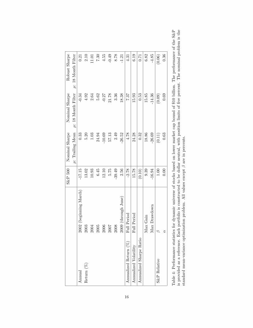
The results of our analysis our found in Table 4. We notice that on an annualized basis each of the activelyconstructed portfolios outperforms the S&P 500 Index, with little � exposure and positive, statisticallysignificant monthly �. We have, however, neglected transaction costs, but these should be to a minimumgiven the universe under consideration.

The more volatile, traditional Sharpe optimized portfolio using a trailing mean for � loses a considerableamount through the middle of 2009. This is likely due to the dramatic reversal in the markets after Marchof that year, and the tendency that we noted earlier for such a portfolio to be trend following. We seeconsiderable outperformance in terms of annualized return (7.37% annualized return) from the nominalproblem using a forecasted return. Further, we see a reduction of annualized volatility relative to thetraditional trailing mean based portfolio. However, the volatility of the forecasted �, Sharpe optimizedportfolio is approximately the same as the market index.

The robust Sharpe portfolio using the 18 month filter forecast for � has a low annualized volatility of just6.19% from 2002-2009. This is coupled with a lower annualized return (relative to the nominal with forecast)of 4.31%. Additionally, this portfolio provides the highest Sharpe ratio among those portfolios consideredhere with a value of 0.71. However, this is essentially the same result obtained for the naive portfolio createdusing this same � (viz., Table 3). This heuristic construction equals or outperforms the traditional Sharpeoptimized portfolio, and provides the most � of all strategies considered. It has a significantly negative yearin 2008, however.

It is interesting to note that every one of the optimal portfolios considered here is positive in 2008, adisastrous year for many equity based investments. Further, the robust portfolio does not see a loss exceeding5% in any month in our history. This is balanced by not having any outsized gains, either. We note thatthis is the intended outcome for such a portfolio.

15

S&

P500

Nom

inal

Sh

arp

eN

om

inal

Sh

arp

eR

ob

ust

Sh

arp

e

�:

Tra

ilin

gM

ean

�:

18

Month

Fil

ter

�:

18

Month

Fil

ter

An

nu

al20

02(b

egin

nin

gM

arc

h)

-17.1

50.3

3-0

.34

0.2

1

Ret

urn

(%)

2003

13.0

25.2

04.9

22.1

0

2004

10.9

31.0

32.6

411.0

1

2005

6.4

524.9

45.6

27.3

0

2006

12.1

0-1

0.6

9-0

.27

4.5

5

2007

5.7

557.1

321.7

8-0

.49

2008

-39.4

92.4

93.3

68.7

8

2009

(th

rou

ghJu

ne)

2.5

6-2

6.5

218.3

8-1

.21

An

nu

aliz

edR

eturn

(%)

Fu

llP

erio

d-2

.78

4.7

87.3

74.3

1

An

nu

aliz

edV

olat

ilit

yF

ull

Per

iod

15.7

824.2

815.9

36.1

9

An

nu

aliz

edS

har

pe

Rat

io(0

.10)

0.3

20.5

30.7

1

Max

Gai

n9.3

918.8

615.8

56.8

2

Max

Dra

wd

own

-16.9

4-2

6.6

9-1

4.3

6-4

.85

S&

PR

elat

ive

�1.0

0(0

.11)

(0.0

9)

(0.0

6)

�0.0

00.6

30.6

90.3

6

Tab

le4:

Per

form

ance

stat

isti

csfo

rd

yn

amic

un

iver

seof

stock

sb

ase

don

low

erm

ark

etca

pb

ou

nd

of

$10

bil

lion

.T

he

per

form

an

ceof

the

S&

Pis

pro

vid

edas

are

fere

nce

.E

ach

por

tfol

iois

con

stru

cted

tob

ed

oll

ar

neu

tral,

wit

hp

osi

tion

lim

its

of

five

per

cent.

Th

en

om

inal

pro

ble

mis

the

stan

dar

dm

ean

-var

ian

ceop

tim

izat

ion

pro

ble

m.

All

valu

esex

cep

t�

are

inp

erce

nts

.

16

Finally, we note that in the end, likely due in part to nonstationarity of covariance, the traditional Sharpeoptimized portfolios (using both a forecast and trailing mean) produce results with lower Sharpe ratios thana simple heuristic method. We believe this is remedied in the robust case, where the methodology contributesin a meaningful way to realistic portfolio construction.

6 Concluding Remarks and Future Work

We tested the performance of the traditional Sharpe optimization problem, and noted both the nonstation-arity of the underlying input parameters as well as the sensitivity of the procedure to perturbations in thosesame inputs. We addressed the latter of these issues using the work of Goldfarb and Iyengar to formulate arobust counterpart to the original problem.

We developed a linear factor model, and conducted cross-sectional regressions to fit the model param-eters. These regression outputs were found to have a term structure. We examined a heuristic portfolioconstruction procedure using lagged filters on the model factor returns to produce forecasted returns. Theseportfolios outperformed the index-based optimized portfolios, and we decided on an 18 month filter basedon its performance. This model was then used to construct uncertainty sets for a robust Sharpe problem.Additionally, we provided another formulation of a robust Sharpe problem, suggesting a new uncertainty setfor the expected return. We did not solve this problem, though.

Our method deviated from Goldfarb and Iyengar in that our regressions were cross-sectional and nottemporal. Therefore, their derivations of their uncertainty sets did not obtain in our case. We producedmodifications to adapt to our regressions. However, we did not rigorously derive or develop said sets.

The performance of the robust Sharpe portfolio using our five-factor linear model was shown to producevery desirable results: very minimal losses, with an attractive Sharpe and positive �. All of the long-shortoptimal portfolios we considered generated positive returns over the period 2002-2009. The traditionalSharpe problem using a trailing mean was the least attractive of the portfolios we considered in almost everysummary statistic we reported: annualized return, volatility, maximum gain, maximum drawdown, Sharperatio, and �.

In future work, we would like to further our development of the uncertainty sets used above. That is, wewould like to produce regression-based uncertainty sets when considering a cross-sectional setting. Further,we would like to implement the new robust problem we formulated. This new problem is attractive in thatit seeks to maintain the correlation structure between returns when considering return uncertainty.

References

[1] V. DeMiguel, L. Garlappi, and R. Uppal. Optimal versus naive diversification: How inefficient is the 1/nportfolio strategy? Review of Financial Studies, 22(5):1915–1953, 2009.

[2] E. Fama and K. French. Common risk factors in the returns on stocks and bonds. Journal of FinancialEconomics, 33:3–56, 1992.

[3] D. Goldfarb and G. Iyengar. Robust portfolio selection problems. Mathematics of Operations Research,28(1):1–38, 2003.

[4] R. A. Haugen and N. L. Bakerb. Commonality in the determinants of expected stock returns. Journalof Financial Economics, 41:401–439, 1996.

17

[5] O. Ledoit and M. Wolf. A well-conditioned estimator for large-dimensional covariance matrices. Journalof Multivariate Analysis, 88:365–411, 2004.

[6] D. N. Nawrocki. Portfolio optimization, heuristics, and the ”butterfly effect”. Journal of FinancialPlanning, pages 68–78, 2000.

[7] J. D. Schwager. Managed Trading: Myths and Truths. Wiley; 1 edition, 1996.

[8] M. Koenig and R. H. Ttnc. Robust asset allocation. Annals of Operations Research, 132:157–187, 2004.

18