Robust Ranging in the Presence of RepeaterSignals

Andreas Iliopoulos∗, Christoph Enneking ∗ ◦, Thomas Jost∗, Omar Garcı́a Crespillo∗ , Manuel Appel ∗ ⊕ and Felix Antreich ∗ ◦,∗ Institute of Communications and Navigation, German Aerospace Center (DLR)◦ Department of Teleinformatics Engineering,Federal University of Ceara (UFC)

⊕ RWTH Aachen University

BIOGRAPHY

Andreas Iliopoulos received his M.Sc. in electrical engineering from the Munich University of Technology (TUM), Germany,in 2012. From 2012 to 2013 he was working as researcher in the Institute for Integrated Systems at the Munich University ofTechnology (TUM). Since 2013 he has been with the Institute of Communications and Navigation at the German AerospaceCenter (DLR). His research interests include statistical signal processing, interference mitigation, wireless communications,antenna array processing, estimation theory and optimization.

Christoph Enneking received his MSc. in electrical engineering from the Munich University of Technology (TUM), Germany,in 2014. In September 2014, he joined the Institute of Communications and Navigation of the German Aerospace Center (DLR).His research interests include GNSS signal design, estimation theory, and GNSS intra- and intersystem interference.

Dr. Thomas Jost received the Diploma degree (FH) in electrical engineering from University of Applied Science Wiesbaden,Germany, in 2001, the Diploma degree in Electrical engineering and information technology from Technical University ofDarmstadt, Germany, in 2003 and the Doctoral degree from University of Vigo, Spain, in 2013. From 2003 to 2006, he held aresearch assistant position in the Signal Processing Group at TU Darmstadt. Since 2006, he is a member of the scientific staff ofthe Institute of Communications and Navigation at the German Aerospace Center.

Omar Garcı́a Crespillo received his M.Sc. in Telecommunication Engineering from the University of Malaga in Spain in2013. In the same year, he joined the Integrity group of the Navigation department of the German Aerospace Center (DLR). Hiscurrent field of research includes GNSS, integrated inertial navigation, Bayesian estimation and integrity. Since 2015, he is alsoa PhD student at the Swiss Federal Institute of Technology (EPFL) in Lausanne.

Manuel Appel received his diploma degree in electrical engineering from the university of applied science Ingolstadt, Germanyin 2008. Additionally he received a M.Sc. degree from Technical University Munich in 2013 after working at FraunhoferInstitute for Integrated Circuits in Erlangen. He joined the Institute for Communication and Navigation of DLR in January 2014.His main research interest is in development of signal processing algorithms for robust GNSS receivers with the main focus onspoofing detection and mitigation.

Dr. Felix Antreich received the Diploma degree in electrical engineering from the Munich University of Technology (TUM),Munich, Germany, in 2003. In 2011 he also received the Doktor-Ingenieur (Ph.D.) degree from the TUM. From 2003 to 2016,he was an Associate Researcher with the Department of Navigation, Institute of Communications and Navigation of the GermanAerospace Center (DLR), Wessling- Oberpfaffenhofen. Since September 2016 he is a visiting professor in the Department ofTeleinformatics Engineering (DETI) at the Federal University of Ceara (UFC) in Fortaleza, Brazil. His research interests includesensor array signal processing for GNSS and wireless communications, estimation theory, wireless sensor networks, and signaldesign for synchronization.

ABSTRACT

This paper tackles the problem of robust Global Navigation Satellite System (GNSS) ranging in the presence of GNSS re-peater signals. In such cases repeater signals act as an interference to live GNSS satellite signals and need to be mitigated.The first contribution of this paper is the impact analysis of repeater signals on Delay-Locked-Loops (DLL), which aretraditionally utilized for the time of arrival estimation in GNSS receivers. In the analysis, we determine different threatregions based on satellite signal and repeater signal parameters. Secondly, it introduces a novel algorithm that performssimultaneous channel estimation and equalization for GNSS signals. The proposed algorithm proves to be resilient inthe presence of GNSS repeater signals in comparison to regular DLL structures. Finally, based on the inherent channelestimation the algorithm provides, it is possible to characterize the parameters of GNSS repeaters.

I INTRODUCTION

Global Navigation Satellite System (GNSS) repeaters are devices designed to receive GNSS signals, amplify them and retransmitthem in enclosed areas. Those devices find various uses in civil applications. For instance, civil aircraft undergoing maintenancein hangars are using repeater signals that are being captured on the roof of a hangar and retransmitted into the hall in order to testtheir avionic systems without leaving the enclosure of the hangar [1]. Recent research has also found usage in repeaters for indoorpositioning and navigation by arranging them in a certain geometry in large buildings and treating them as ”repeaterlites” [2].Aside from their aforementioned benefits, GNSS repeaters can introduce a significant hazard. That usually occurs in the case ofsimultaneous existence of GNSS satellite signals and repeated signals. Then, repeated signals are viewed as interference insteadof beneficial signals. Repeated signals have inherently a larger travel distance than the direct Line-of-Sight (LOS) signals and actas interference to the Delay-Locked-Loop (DLL). Additionally, repeater signals are amplified before transmission which posesan additional challenge. The amplified repeated signals have usually a much higher power than regular live GNSS signals andthus usually dominate them. Furthermore, by amplifying the live signals, repeater devices simultaneously amplify environmentalnoise as well as thermal noise from the reception antenna and the amplifiers. The latter has a profound effect on regular GNSSrepeater signals, since the noise amplification acts as an Additive White Gaussian-Noise (AWGN) jammer.The combined effect of GNSS signal shadowing and jamming can lead to disastrous results. Depending on the repeater set upparameters, regular GNSS receivers can produce a large variance in their positioning solution, provide no positioning solution atall and more importantly produce a falsified position. In the last case, the repeated signals have such a low power to go undetectedyet large enough to dominate the live signals. As a result, the GNSS receiver will estimate a range that approximately correspondsto the site of the repeater reception antenna and hereby estimate the position of the reception antenna as its own. Usually, suchphenomena go undetected in civil applications. However, there are instances, where repeaters have posed a significant risk forsafety critical applications, most importantly for avionic applications. In 2010, at Hannover airport, a GNSS repeater installed ina hangar caused problems to aircraft that were taxiing and taking off [3]. The interference was reported to have caused alerts andalarms with aircraft systems at ranges up to several hundred meters from the hangar.The structure of this paper is as follows. In Section II, we conduct a study on the current repeater mitigation options and weconduct a literature review on Extended Kalman Filter (EKF) based satellite signal code delay algorithms. In Section III, weperform a threat analysis of the repeater interference on the widely utilized Delay-Locked-Loops(DLLs) in the GNSS community.Section IV introduces the developed signal model, which is used in Section V to describe the proposed mitigation algorithm.Finally, in Section VI, we show the mitigation performance of the proposed algorithm by simulations.

II STATE OF THE ART

Currently the usage of GNSS repeaters is strongly regulated. International Civil Aviation Organization (ICAO) member stateshave to ensure that the interference is controlled and in line with the requirements of [4]. Thus, repeater manufacturers andoperators have to be aware and follow certain regulations. The aforementioned examples however indicate that regulation cannotcompletely protect against interference-like repeated signals.Other countermeasures against repeaters serve solely as detectors that identify the existence of repeaters in the intermediate area.This can be achieved through different techniques. The first and easiest includes interference monitoring through investigation ofthe power spectral density of the designated GNSS bands. A different category includes the determination of different interferencemetrics in a customized GNSS receiver. Those can include the Delta Metric [5], Ratio Metric [5], Early-Late Phase Metric [6],Magnitude-Difference Metric [7].An additional methodology for repeater detection and characterization includes the implementation of Receiver AutonomousIntegrity Monitor (RAIM) algorithms [8]. Those algorithms can either estimate inconsistencies in GNSS signals by generatingsubsets of the measured satellite signals and by processing different GNSS signal frequencies and comparing them [9].

Kalman filters utilization in the GNSS context has found many applications. The most wide spread usage of them in the GNSScommunity is the coupling different satellite tracking modules, which in turn increases overall tracking robustness [10]. Adifferent usage is coupling Delay/Phase Locked Loops (DLL/PLL) strucutres with inertial sensors in order to provide navigationinformation under harsh conditions and even in the absence of GNSS signals [11].The use of Extended Kalman Filter (EKF) for code delay/channel estimation in signal tracking was first introduced in communi-cations by [12,13]. In both cases the introduced structure is in the pre-correlation domain, assuming short Code Division MultipleAccess (CDMA) code lengths and Signal-to-Noise Ratio (SNR) many orders of magnitude higher than in GNSS. The placementof post-correlation EKF has been studied in the GNSS community. In [14], the authors utilize prompt and discriminator outputsas EKF measurements for carrier phase, code phase and carrier amplitude determination. Similar work was presented in [15],where interleaved but separate EKFs are used that include regular early, late and prompt correlators as input as well as Doppler,acceleration and phase information for stable delay code tracking under harsh SNR conditions. Finally, [16] presents a methodto jointly estimate code delays and channel coefficients using EKF coupled with an interference cancellation scheme and teststatistics for the case of a multicell CDMA transmission scheme.A systematic approach of a correlator bank usage for parameter estimation was suggested by Selva [17] and is suited for parameterestimation in multipath environments. The use of a correlator bank reduces sample sizes considerably, so that estimation of apotentially large number of parameters in digital signal processing becomes computationally affordable as long as the datadepends linearly on most of the parameters. This methodology has since been adopted in many works on GNSS parameterestimation for multipath scenarios. These works include estimation or tracking of multiple signal arrivals, optimality criteriabeing ML [18], Bayesian mean squared error [19] or mixtures of the two [20, 21].In [22], we presented a novel algorithm based on the EKF, which substitutes traditional DLLs and is able to robustly track thesatellite signal code delay and simultaneously estimate the GNSS signal channel, with the help of a multicorrelator bank structure.In this paper, we optimize the aforementioned algorithm and further develop it to also handle and estimate complex amplitudesof the signals contained in the channel seen by a GNSS receiver.

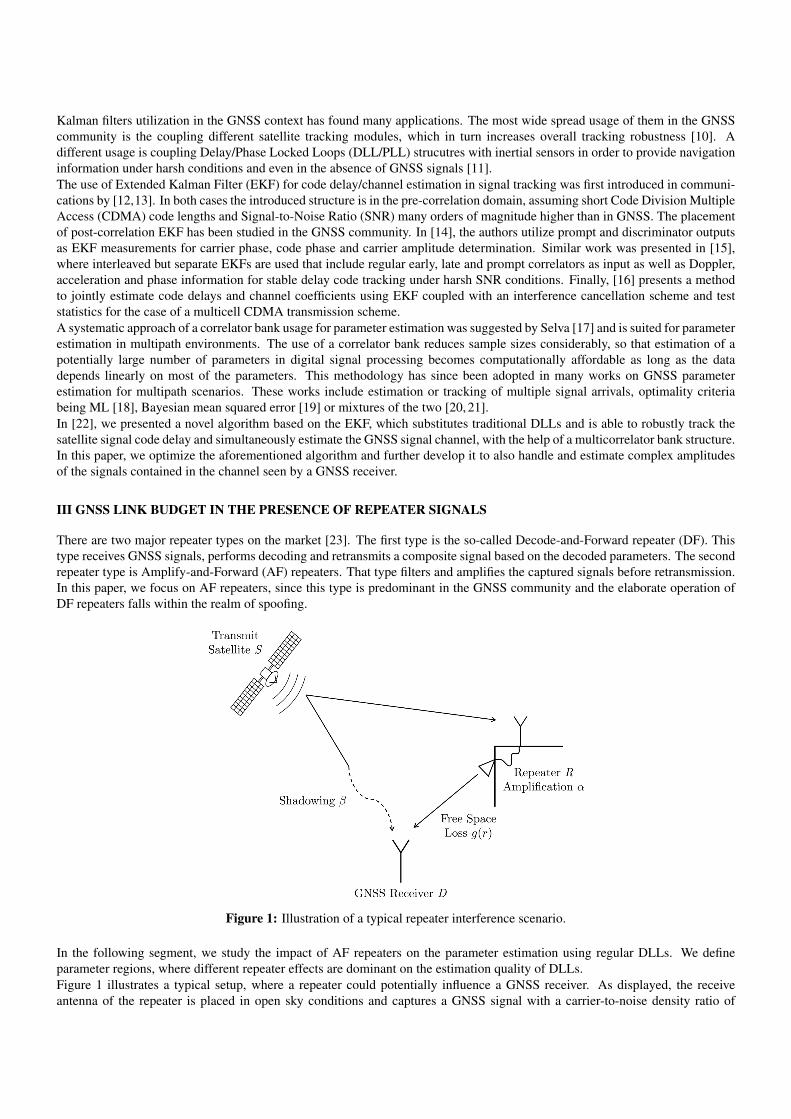
III GNSS LINK BUDGET IN THE PRESENCE OF REPEATER SIGNALS

There are two major repeater types on the market [23]. The first type is the so-called Decode-and-Forward repeater (DF). Thistype receives GNSS signals, performs decoding and retransmits a composite signal based on the decoded parameters. The secondrepeater type is Amplify-and-Forward (AF) repeaters. That type filters and amplifies the captured signals before retransmission.In this paper, we focus on AF repeaters, since this type is predominant in the GNSS community and the elaborate operation ofDF repeaters falls within the realm of spoofing.

Figure 1: Illustration of a typical repeater interference scenario.

In the following segment, we study the impact of AF repeaters on the parameter estimation using regular DLLs. We defineparameter regions, where different repeater effects are dominant on the estimation quality of DLLs.Figure 1 illustrates a typical setup, where a repeater could potentially influence a GNSS receiver. As displayed, the receiveantenna of the repeater is placed in open sky conditions and captures a GNSS signal with a carrier-to-noise density ratio of

C/N0. The captured signal is then filtered and amplified with an amplification factor α before being re-transmitted to a localarea, such as a hangar, a mall or similar. After transmission, the repeater signal is attenuated by Free-Space-Loss (FSL) accordingto

g(r) =

(c

4πrfLi

)2

, (1)

where r stands for the repeater-destination distance, fLi the signal carrier frequency and c the speed of light. As seen in Equation(1), FSL decreases with distance r as well as with the signal frequency fLi.A GNSS receiver located outside of the building with the installed repeater will see the Line-of-Sight (LOS) signal with a carrier-to-noise ratio of βC/N0 due to shadowing effects. The attenuation factor β ≤ 1 represents shadowing and varies between βminand 1. β = 1 indicates that the GNSS receiver has open sky conditions and sees the same C/N0 as the repeater. β = βminillustrates the case where shadowing is so severe that the GNSS receiver sees the minimum guaranteed signal power [24].In case the repeater signal escapes the building enclosure, it experiences a net amplification of αg(r) and acts as interference tothe nominal operation of the GNSS receiver.

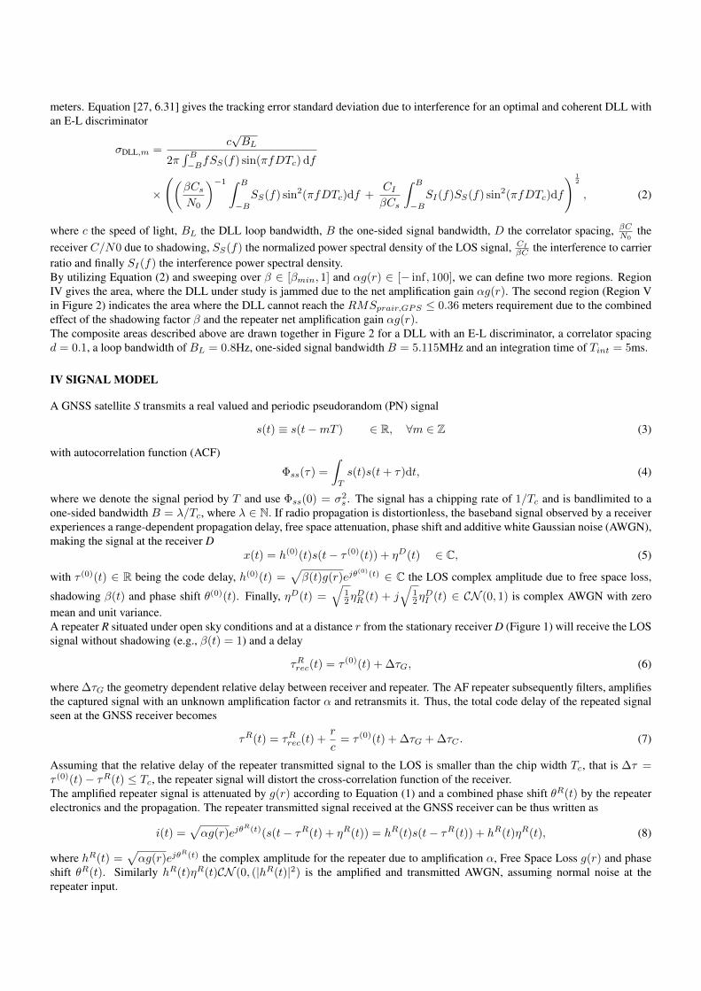
Figure 2: Illustration of dominant repeater effect regions.

If the free space loss overpowers the repeater amplification and the net power of the repeated signal αg(r) is less than 0.01, thenthe receiver DLL is assumed to be operating in nominal conditions (Region I in Figure 2).If the amplification of the repeater is stronger or is the receiver is closer to the transmit antenna of the repeater, the net amplifica-tion of the repeated signal get stronger. We assume that if the net amplification varies between 0.01 and the shadowing value ofβ, then the repeated signal affects the receiver DLL and behaves similar to multipath (Region II in Figure 2).When the net amplification reaches β, any gain from the LNA amplification is negated by the FSL. That means that the repeatedsignal has the same power as the LOS signal and thus a DLL cannot differentiate between the actual LOS and the ”counterfeit”signal.The differentiation becomes even more difficult, if the net amplification of the repeated signal seen at the GNSS receiver exceedsβ. At that point (Region III in Figure 2), the repeated signal dominates the actual LOS and the DLL of the GNSS receivereventually locks to the stronger repeated signal.If the repeater signal power further increases, an interesting effect takes place. The repeater does not only amplify GNSS signalsbut also its thermal white Gaussian noise. Therefore, the repeater signal leads to an increase of the noise floor due to the noisefigure of the repeater electronics. Thus, if the net amplification seen at the GNSS receiver exceeds a certain value, the GNSSreceiver cannot work satisfactorily, even if it completely mitigates the effect of the repeater signal. The reason is that over acertain threshold, the noise amplification caused by the repeater acts as an Additive-White-Gaussian-Noise (AWGN) jammerand thus anti-jamming signal processing algorithms are required before dealing with the repeated GNSS signal. But what netamplification leads to such a jamming effect on the GNSS receiver?Before dealing with that question, we have to define what constitutes a jammer in the GNSS framework and what are theminimum ranging degradation a DLL can endure before being characterized as being jammed.In [25, Appendix-H] an indication is given on what constitutes jamming by defining power masks within the L-band based onthe bandwidth of the jamming signal. This way however, we cannot associate the jammer’s influence on the DLL operation. [26,S.2.1.4.1.4] defines a more concrete metric for aeronautical applications and specifies a ranging error RMSair,GPS ≤ 0.36

meters. Equation [27, 6.31] gives the tracking error standard deviation due to interference for an optimal and coherent DLL withan E-L discriminator

σDLL,m =c√BL

2π∫ B−BfSS(f) sin(πfDTc) df

×

((βCsN0

)−1 ∫ B

−BSS(f) sin2(πfDTc)df +

CIβCs

∫ B

−BSI(f)SS(f) sin2(πfDTc)df

) 12

, (2)

where c the speed of light, BL the DLL loop bandwidth, B the one-sided signal bandwidth, D the correlator spacing, βCN0the

receiver C/N0 due to shadowing, SS(f) the normalized power spectral density of the LOS signal, CI

βC the interference to carrierratio and finally SI(f) the interference power spectral density.By utilizing Equation (2) and sweeping over β ∈ [βmin, 1] and αg(r) ∈ [− inf, 100], we can define two more regions. RegionIV gives the area, where the DLL under study is jammed due to the net amplification gain αg(r). The second region (Region Vin Figure 2) indicates the area where the DLL cannot reach the RMSprair,GPS ≤ 0.36 meters requirement due to the combinedeffect of the shadowing factor β and the repeater net amplification gain αg(r).The composite areas described above are drawn together in Figure 2 for a DLL with an E-L discriminator, a correlator spacingd = 0.1, a loop bandwidth of BL = 0.8Hz, one-sided signal bandwidth B = 5.115MHz and an integration time of Tint = 5ms.

IV SIGNAL MODEL

A GNSS satellite S transmits a real valued and periodic pseudorandom (PN) signal

s(t) ≡ s(t−mT ) ∈ R, ∀m ∈ Z (3)

with autocorrelation function (ACF)

Φss(τ) =

∫T

s(t)s(t+ τ)dt, (4)

where we denote the signal period by T and use Φss(0) = σ2s . The signal has a chipping rate of 1/Tc and is bandlimited to a

one-sided bandwidth B = λ/Tc, where λ ∈ N. If radio propagation is distortionless, the baseband signal observed by a receiverexperiences a range-dependent propagation delay, free space attenuation, phase shift and additive white Gaussian noise (AWGN),making the signal at the receiver D

x(t) = h(0)(t)s(t− τ (0)(t)) + ηD(t) ∈ C, (5)

with τ (0)(t) ∈ R being the code delay, h(0)(t) =√β(t)g(r)ejθ

(0)(t) ∈ C the LOS complex amplitude due to free space loss,

shadowing β(t) and phase shift θ(0)(t). Finally, ηD(t) =√

12ηDR (t) + j

√12ηDI (t) ∈ CN (0, 1) is complex AWGN with zero

mean and unit variance.A repeater R situated under open sky conditions and at a distance r from the stationary receiver D (Figure 1) will receive the LOSsignal without shadowing (e.g., β(t) = 1) and a delay

τRrec(t) = τ (0)(t) + ∆τG, (6)

where ∆τG the geometry dependent relative delay between receiver and repeater. The AF repeater subsequently filters, amplifiesthe captured signal with an unknown amplification factor α and retransmits it. Thus, the total code delay of the repeated signalseen at the GNSS receiver becomes

τR(t) = τRrec(t) +r

c= τ (0)(t) + ∆τG + ∆τC . (7)

Assuming that the relative delay of the repeater transmitted signal to the LOS is smaller than the chip width Tc, that is ∆τ =τ (0)(t)− τR(t) ≤ Tc, the repeater signal will distort the cross-correlation function of the receiver.The amplified repeater signal is attenuated by g(r) according to Equation (1) and a combined phase shift θR(t) by the repeaterelectronics and the propagation. The repeater transmitted signal received at the GNSS receiver can be thus written as

i(t) =√αg(r)ejθ

R(t)(s(t− τR(t) + ηR(t)) = hR(t)s(t− τR(t)) + hR(t)ηR(t), (8)

where hR(t) =√αg(r)ejθ

R(t) the complex amplitude for the repeater due to amplification α, Free Space Loss g(r) and phaseshift θR(t). Similarly hR(t)ηR(t)CN (0, (|hR(t)|2) is the amplified and transmitted AWGN, assuming normal noise at therepeater input.

The received signal containing the LOS to the satellite, the repeater signal and the AWGN can be thus expressed as

y(t) = x(t) + i(t)

= h(0)(t)s(t− τ (0)(t)) + hR(t)s(t− τR(t)) + ηD(t) + hR(t)ηR(t)

= h(0)(t)s(t− τ (0)(t)) + hR(t)s(t− τR(t)) + η(t), (9)

since the sum of of the two complex AWGN sources, (ηD ∈ CN (0, 1) and ηR ∈ CN (0, (|hR(t)|2)) will also produce an AWGNη ∈ CN (0, (|hR(t)|2+1)).We approximate the complex amplitudes of the signals and their respective delays by a tap delay line channel coefficients withDirac distributions that are equidistantly arranged in time

h(t, τ) ≈L∑`=0

h(`)(t)δ(τ − `Ts) (10)

with time-variant weights h(`)(t). That is a valid assumption when the sampling period Ts is significantly smaller than the chipduration Tc, that is Ts � Tc and L satisfying LTs = Tc. Inserting (10) into (9), we get

y(t) ≈L∑`=0

h(`)k s(t− τ (0)k − `Ts) + η(t). (11)

Since the channel coherence time (i.e. the time where the channel parameters remains quasi-constant) is typically larger than thecoherent integration time TNc over Nc PN periods T , the last approximation in the equation above is that the LOS delay and thechannel weights are block-wise constant, τ (0)k , τ (0)(kTNc) and h(`)k , h(`)(kTNc) and ` = 0, . . . , L for

k = b t

TNcc = b t

TsNNcc = b t

TsMc (12)

with M = NNc the number of samples in one coherent integration period.As a next processing step, the received signal is lowpass filtered with one-sided bandwidth B and sampled at the Nyquist rate1Ts

= 2B. The design parameter λ, representing the oversampling factor, can be chosen sufficiently high to satisfy Ts � Tc.The number of observable channel coefficients is then L = Tc

Ts= 2λ. Sampling the signal in (11) for the n-th sample of the k-th

coherent integration period leads to

yk[n] , y((kM + n)Ts

)=

L∑`=0

h(`)k s((kM + n)Ts − τ (0)k − `Ts) + η((kM + n)Ts)

=

L∑`=0

h(`)k s((n− `)Ts − τ (0)k ) + η((kM + n)Ts), (13)

where the periodicity of the PN sequence s(t) is exploited (Equation (3)). Collecting periods k = 0, 1, . . . and stacking Msamples per period in one column vector leads to

yk = [yk[1], . . . , yk[M ]]H ∈ CM×1, k = 0, 1, . . . (14)

Thus, our discrete signal can be written in matrix-vector notation as

yk = Hks(τ(0)k ) + ηk, (15)

with the ideal transmit PN signal

s(τ(0)k ) =

s(Ts − τ (0)k )

s(2Ts − τ (0)k )

...

s(MTs − τ (0)k )

∈ CM×1

and the white circular symmetric normal distributed noise term

ηk = [η(Ts + kT ), . . . , η(MTs + kT )]H ∈ CM×1. (16)

The channel in Equation (15) is expressed by a convolution matrix with circulant Toeplitz structure

Hk =

L∑`=0

h(`)k Z

` ∈ CM×M , (17)

with Z being the polynomial basis of the [M ×M ] circulant matrix

Z =

(0H 1

I 0

)∈ RM×M , (18)

where I ∈ R(M−1)×(M−1) stands for an identity matrix, and 0 ∈ R(M−1)×1 a vector containing only zeros.The unknown time-varying signal and channel parameters are summarized by the state vector

xk =[τ(0)k , h

(0)k , h

(1)k , . . . , h

(L)k

]H∈ C(L+2)×1, (19)

containing the real valued LOS delay and the complex valued channel coefficients.

V PROPOSED ALGORITHM

Measurement Model - Multicorrelator Bank

The number of data M collected per coherent integration period k proves to be computationally challenging. Thus, we needan efficient representation of the incoming signal without loss of information. In order to do so, we employ a projection of theobserved signal to a much smaller space, thus reducing the subsequent processing requirements. A variant of these projections isemploying a bank of signal-matched correlators and building the temporal cross-correlation function of the incoming signal witha local set of time shifted replicas [17]

1⊗

sH(τ̂(−q)k )

sH(τ̂(−q+1)k )

...

sH(τ̂(0)k )

...

sH(τ̂(q−1)k )

sH(τ̂(q)k )

yk ∈ CP×1, (20)

where 1 ∈ R1×Nc represents a vector containing ones and is responsible for the coherent integration, ⊗ the Kronecker productoperator, s( · ) ∈ CN×1 represents the sampled PN signal s(t), τ̂ (q)k ∈ R represents the temporal delay of the q-th local PNreplica and P = 2q + 1 is the total number of local replicas. Through this operation, we project the signal from a CM×1 spaceto a much smaller CP×1 space. In order to minimize the loss of information due to reduced dimensionality, we assume that thecorrelator bank’s middle/prompt replica is roughly synchronized with the code delay of the LOS signal, i.e., |τ̂ (0)k − τ

(0)k |≤ Tc/2.

Additionally, we place the remaining 2q correlators symmetrically and equidistantly around the prompt correlator within ±Tcusing a spacing of ∆ = Tc

q . Thus we have

τ̂(±i)k − τ̂ (0)k = ±i∆, i = 1, . . . , q. (21)

This simplifies the parameters that describe the correlator bank

QH(τ̂(0)k ) , 1⊗

sH(τ̂(0)k − q∆)

sH(τ̂(0)k − (q − 1)∆)

...

sH(τ̂(0)k )

...

sH(τ̂(0)k + (q − 1)∆)

sH(τ̂(0)k + q∆)

∈ CP×M , (22)

which is now determined only by ∆, that is the temporal spacing of adjacent correlators, and τ̂ (0)k ∈ R the estimated real valueddelay of the LOS signal. The result of the cross-correlation yields the post-correlation signal

zk = QH(τ̂(0)k )yk = QH(τ̂

(0)k )Hks(τ

(0)k ) +QH(τ̂

(0)k )ηk (23)

for k = 0, 1, . . .

Extended Kalman Filter Description

The received signal yk in the absence of noise can be fully described given the state xk ∈ CL+2 from (19). Thus, given amulticorrelator bank, we set the correlator spacing ∆ = Ts, which results in a number P = 2L+ 1 of correlators. This way, weare able to align the L+ 1 correlators, that is the ”prompt” and the ”late” part of the bank, with the channel Hk experienced bythe satellite signal s(τ (0)k ). In the following, we propose a post-correlation EKF which for each k = 0, 1, . . . estimates the statevector xk based on minimizing the mean square error using the measurements z0, . . . ,zk.The channel coefficients h(`)k and LOS delay τ (0)k are assumed to be independent and the state transition of the EKF algorithmfollows a random walk dynamic model

τ(0)−k = ατ τ

(0)+k−1 + uτ,k (24)

h(`)−k = α

(`)h h

(`)+k−1 + u

(`)h,k ∀` = 0, 1, . . . , L, (25)

where τ (0)−k , h(`)−k is the filter prediction of the code delay and complex amplitude for the coherent integration k, τ (0)+k−1 , h

(`)+k−1

the filter update of the code delay and complex amplitude for the coherent integration k − 1. uτ,k and u(`)h,k are mutually

independent additive white Gaussian noise processes with variances βτ and β(`)h . State transition model and measurement model

can be written more compactly using the state prediction x−k of the coherent period k and the state update x+k−1 of the coherent

integration period k − 1as

x−k = Ax+k−1 + uk (26)

τ−ref,k = <(τ(0)−k ) (27)

zk = f(xk, τ−ref,k,ηk) (28)

with the state transition matrixA containing the forgetting factors for delay ατ and for the channel taps αh(i)

A =

ατ 0 0 . . . 0

0 αh(0) 0 . . . 0

0 0 αh(1) . . . 0

......

.... . . 0

0 0 . . . 0 αh(L)

(29)

and the process noise vectoruk = [uτ,k, u

(0)h,k, u

(1)h,k, . . . , u

(L)h,k ]H . (30)

The process noise covariance matrix is defined as

B , E[ukuHk ] =

βτ 0 0 . . . 0

0 βh(0) 0 . . . 0

0 0 βh(1) . . . 0

......

.... . . 0

0 0 . . . 0 βh(L)

. (31)

The nonlinear measurement function is given by

zk = f(xk, τ−ref,k,ηk) = QH(τ−ref,k)

[Hksk(τ

(0)k ) + ηk

], (32)

where τ−ref,k denotes the real part of the LOS delay prediction τ (0)k (Equation 27). The estimates for τ (0)k are in general complexdue to the complex valued measurements zk. However, the physical true delay is real valued. In order to overcome a similarproblem, [13] introduces a correction term in the innovation derivation of his EKF depending on the predicted imaginary part ofhis LOS delay estimate. This way, the LOS delay update estimate is forced to become real. In this paper however, we pursuita different but equivalent method. We can let the LOS delay estimation become complex but constrain the predicted delayestimation, which drives the correlator bank, to be real valued. Allowing the imaginary part to run free and driving the bankwith the real valued part of the delay estimation achieves the same result while at the same time omitting the computation of acumbersome correction term. It is important to notice that at time k, the measurement zk depends not only on noise and the truestate xk, but also on the current prompt delay of the correlator bank. For instance, if the prompt delay deviates from the true LOSdelay by more than Tc, the measurement will be independent of the state vector. We assume that the correlator bank’s promptdelay to calculate zk is driven by the best current estimate, which is the prediction τ (0)−k .

A. Prediction Stage

In the joint delay and channel estimation and tracking problem, the system model is linear as shown above. Thus, the EKFequations for the state prediction and associated covariance are

x−k = Ax+k−1 (33)

P−k = AP+k−1A

H +B, (34)

where P+k−1 is the covariance associated with the EKF’s state estimate at the end of the previous iteration (update). Further, the

predicted measurement is defined as

z−k = E {zk|zk−1, . . . ,z0} = E{zk|x−k

}= f(x−k ,x

−k ,0) (35)

which is equivalent to the measurement function evaluated at the predicted state vector x−k .

B. Update Stage

The residual between measurement and predicted measurement is defined as

εk = zk − z−k . (36)

The computed predicted measurement z−k can be computed using the measurement function in (32)

z−k = f(xk, τ−ref,k,0) = QH(τ−ref,k)

[Hksk(τ

(0)k )]. (37)

Assuming that the code delay model is well matched and that the satellite signal code delay does not change significantly withinone coherent integration period, we have

τ−ref,k ≈ τ(0)k . (38)

By exploiting Equation (38) and the relationship sH(τ)s(τ + n∆) = Φss(n∆) for any n ∈ Z, τ ∈ R, we can simplify theexpression for the predicted measurement as

z−k = QH(τ−ref,k)Hksk(τ(0)k )

=

L∑`=0

h(`)−k QH(τ−ref,k)Z`ksk(τ

(0)k )

=

L∑`=0

h(`)−k QH(0)Z`ksk(0)

=

L∑`=0

h(`)−k

Φss((`+ q)∆)

...Φss((`− q)∆)

(39)

That means that the inner term of Equation (39) needs to be calculated once and subsequently only updated accordingly with thepredicted complex amplitudes.From the residual, the updated state estimate and associated covariance are obtained as

x+k = x−k +Kkεk (40)

P+k = (I −KkFk)P−k (41)

with the Kalman gain

Kk = P−k FHk S

−1k ∈ C(L+2)×P , (42)

the residual covariance matrix

Sk = FkP−k F

Hk + VkRkV

Hk . (43)

The linearization of (32) with respect to the state, evaluated at the predicted state vector, provides matrix Fk i.e.,

Fk ,∂f(xk, τ

−ref,k,0)

∂x∗k

∣∣∣∣∣xk=x−

k

=

∂fH(xk,τ−ref,k,0)

∂τ∗(0)k

∂fH(xk,τ−ref,k,0)

∂h∗(0)k

...∂fH(xk,τ

−ref,k,0)

∂h∗(L)k

H ∣∣∣∣∣∣∣∣∣∣∣∣∣∣∣xk=x−

k

∈ CP×(L+2).

The partial derivative in (44) with respect to τ (0)k can be calculated as

∂f(xk, τ−ref,k,0)

∂τ∗(0)k

∣∣∣∣∣xk=x−

k

= QH(τ−ref,k)Hk∂s(τ

(0)k )

∂τ(0)k

∣∣∣∣∣τ(0)k =τ−

ref,k

(44)

Similar to Equation 39, we exploit the relationship sH(τ)s(τ + n∆) = Φss(n∆) for any n ∈Z, τ ∈ R and use (4) and (17),(44) to further simplify the measurement function derivative with respect to code delay. Thus, equation (44) becomes

∂f(xk, τ−ref,k,0)

∂τ∗(0)k

∣∣∣∣∣xk=x−

k

=

L∑`=0

h(`)−k

Φ′ss((`+ q)∆)

...Φ′ss((`− q)∆)

, (45)

where Φ′ss(τ) = ddτΦss(τ).

Likewise, we calculate the partial derivative in (44) with respect to h∗(`)k for ` = 0, . . . , L

∂f(xk, τ−ref,k,0)

∂h∗(`)k

∣∣∣∣∣xk=x−

k

= QH(τ−ref,k)Z`s(τ−ref,k)

= QH(0)Z`s(0)

=

Φss((`+ q)∆)

...Φss((`− q)∆)

. (46)

It is worth noting that (46) does not depend on the prompt delay, hence is time-invariant. Thus, the L + 1 last columns of Fkneed to be calculated only once. On the other hand (45) can be expressed as a weighted sum of vectors with fixed vectors andtime-variant weights, thus it needs to be updated at every measurement epoch with the predicted channel coefficient estimates.Since the pre-correlation noise ηk has i.i.d. standard normally distributed entries, the measurement noise covariance matrix isgiven as

Rk = QH(<(τ(0)−k ))E[ηHk ηk]Q(<(τ

(0)−k ))

= QH(<(τ(0)−k ))E[ηHk ηk]Q(<(τ

(0)−k ))

= QH(0)E[ηHk ηk]Q(0)

= (1 + |hR−k |2)

Φss(0) . . . Φss(2q∆)

.... . .

...Φss(2q∆) . . . Φss(0)

, (47)

where |hR−k |2 corresponds to the interpolated and absolute squared predicted channel coefficient of the repeater in the channel.If the repeater is off or located outside the correlator bank, then |hR−k |2 → 0 and we have nominal operation for the proposedscheme. Also it is important to notice that the post-correlation measurement noise vector QH(τ−ref,k)ηk has correlated entriesdespite ηk having i.i.d. entries. Due to multiplication with the correlator bank, the measurement noise of the EKF is coloredwith covarianceRk.

C. Algorithm Discussion - Implementation Analysis

In the following, we discuss the requirements for a possible implementation of the proposed algorithm.Traditional DLLs would feed the incoming signal yk to a ”Correlator Bank” block containing a number of time shifted replicasof the PN sequence. The results of the cross-correlation operation is coherently integrated in the ”Integrate & Dump”, whichproduces a measurement every Nc integration periods. Its integrated correlator outputs are combined to calculate the delaycorrection for the current measurement epoch with the usage of a discriminator function. DLLs subsequently filter their discrim-inator output with a low-pass filter and may also utilize carrier-aiding to further smooth the delay correction. Next, they translatethe calculated correction to a NCO rate update by which they control the PRN generator of the GNSS receiver. The updated PRNreplica is finally used to close the DLL loop and perform the cross-correlation operation with the incoming signal at the nextintegration period.Figure 3 illustrates the adaptations that need to be carried out in order to implement the proposed algorithm in the place of a”traditional” DLL.The proposed algorithm requires a bank with P correlators according to Equation (22), whose number depends on the front-endbandwidth. This requires more computational resources than the regular three ”early-prompt-late” correlators in a DLL but it iscomparable for small front-end bandwidths the computational effort required for other discriminators such as the double deltadiscriminators. As seen in Figure 3, the proposed algorithm substitutes the discriminator function and the low-pass filter withan EKF filter. It tracks the form of the cross-correlation function by comparing the estimated cross-correlation function with themeasurement zk. Contrary to other extended Kalman filter implementations, the proposed scheme does not need to recalculatethe predicted measurement or the measurement function partial derivative with respect to the complex amplitudes. Those remainconstant and thus can be calculated at start-up and then stored in a Look-Up-Table (LUT). Similarly, the partial derivative withrespect to delay and the measurement noise covariance matrix, only need to be updated with the current complex amplitudepredictions. Thus, they also can be saved in a LUT and refreshed at every update iteration of the propose scheme. Overall, the

Figure 3: Block-wise visualization of the proposed EKF scheme.

internal EKF computations involve small matrix multiplications, additions and one inversion at a low rate, which depends on theintegration time chosen, which can be handled with a small overhead in comparison to regular DLLs. As already mentioned, themain bottleneck of the algorithm remains the high number of correlators required in the bank for large front-end bandwidths.

VI SIMULATIVE RESULTS

In order to test the capabilities of the algorithm proposed, we carried out computer simulations to demonstrate its LOS delayand channel coefficients estimation capabilities. For the following simulation scenario, we choose λ = 5. Therefore, thenominal signal has single-sided bandwidth B = λ/Tc = 5.115MHz, is sampled with the Nyquist frequency frequency fs =2λTc

= 10.23MHz and subsequently cross-correlated with a correlator bank containing a total of P = 2L + 1 = 21 equispacedcorrelators with a spacing of ∆ = 2Tc

L = 0.1Tc. The nominal carrier-to-noise density (i.e. C0

No) is set to 42dB-Hz, the LOS

phase θ0k = 0 and therefore its LOS channel coefficient starts at h(0)0 =√

C0

NoB= 0.0557. The received signal is subsequently

cross-correlated and coherently integrated overNc = 5 epochs. Thus, the effectiveC/N0′ = C/N0+10log10(Nc) = 49dB-Hz.The initial delay estimation error is τ (0)0 − τ (0)+0 = 0.0Tc, modeling stable tracking behavior, and the initial amplitude error ish(0)0 − h

(0)+0 = 0.0, thus assuming accurate initial guess. The associated standard deviation of the initial guess is 0.5Tc for the

LOS delay and 0.1 for all amplitudes. Hereafter, the ground truth delay and amplitude of the LOS signal perform a random walk

as defined in Equations (24-31) with A = I ,√βτ = 0.001Tc and

√β(`)h = 0.01 for ` = 0, . . . , L. The EKF utilizes Ncβτ for

the delay process noise and respectively Ncβ(`)h for the coefficient process noise to account for the accumulated noise over the

coherent integration time. For comparison, a second order DLL with an early-late spacing of 0.2Tc, a loop bandwidth of 0.8 Hzand a normalized early-minus-late discriminator has been implemented and tested for the same scenario.

Sudden Repeater Interference

In the following, we investigate a scenario with a sudden start of AF repeater interference corresponding to the example in Figure1. For the first 500ms the GNSS receiver only receives LOS satellite signals. After that, the signal of an AF repeater located at adistance of r = 80m and with an α = 77.5dB amplification is received and interferes with nominal GNSS reception. Based on(1), the repeated signal undergoes a free space loss g(r) = 74.5dB and thus the net amplification gain becomes αg(r) = 3dB.Additionally, the repeater signal arrives with a relative phase difference ∆θ = θ0k − θRk = π

4 respective to the LOS, meaning thatthe repeated signal power is split equally between the in-phase and the quadrature channel seen at the receiver. It is interestingto note that since the resulting C/N0 at the receiver is 49dB-Hz and the net amplification gain of the repeater αg(r) = 3dB, aGNSS receiver with a ”traditional” DLL estimator would experience effects corresponding to Region III in Figure (2). Thus, weexpect that the DLL would track the repeated signal instead of the satellite signal.

Figure 4: Comparison of the real LOS delay with the DLL and EKF based estimate.

Figure (4) illustrates the influence of the repeated signal on the delay estimation. In the first 500ms both the traditional DLL andthe proposed algorithm are able to perfectly follow the random walk that the ground truth delay is undergoing. However, as soonas the repeater signal is introduced, the traditional DLL experiences a delay bias due to its effect. That is since the repeated signalreplica is 3dB stronger than the LOS and arrives with a relative delay equal to ∆τ = r

cTc= 0.273 chips. As a matter of fact, the

bias to the ground truth for the regular DLL is approximately 0.27 chips as it can be seen in Figure (4). The proposed algorithmhowever appears to be immune to the repeater effect and is able to accurately track the ground truth delay.

Figure 5: Comparison of the real and estimated LOS amplitude.

Figure (5) shows the estimation and ground truth for the LOS channel coefficient. It can be seen that proposed algorithm is ableto estimate and track the behavior of LOS with a small variance in the first 500ms. As soon as the repeater signal is turned on,the proposed algorithm is still able to track the LOS amplitude but the variance of the estimation is increased due to the increasednoise introduced by the repeater.As it can be seen from Figure (6), the proposed algorithm converges and keeps the relative error for both the LOS delay andamplitude estimation small and well bounded. This can be inferred by the 3στ and 3σh0 standard deviations for LOS delay andamplitude, which can be extracted by the respective elements of the state covariance matrix Pk. Both of them quickly convergeto a steady value and confidently over-bound the respective calculated absolute errors for delay and amplitude estimation.Figure (7-8) show the respective estimates of the inphase and quadrature Channel Impulse Responses (CIR) over time and delay.As it can be seen from Figure (7), at the start of the simulation, the LOS is dominant and centered around 0Tc delay. All thesubsequent channel coefficient estimates have a noise-like behaviour. Since the LOS phase θ0k is set to zero, the LOS is purely

Figure 6: LOS delay and amplitude estimation error over their respective 3σ variances.

Figure 7: Visualization of the interpolated inphase CIR.

real. Thus, it appears in the inphase part of the channel (Figure 7) and only noise can be observed in the quadrature (Figure 8).After 500ms, the repeater is turned on and the proposed algorithm adapts to the joint LOS and repeater signal presence. It isable to estimate the repeater presence between the channel tabs h(2)k and h(3)k , which correspond to a 0.2 and 0.3 relative chipdelay with respect to the LOS. Due to the repeaters relative phase ∆θ = π

4 , the repeated signal appears in both the inphaseand quadrature channel impulse response. Furthermore, as Figure 7-Figure 8 indicate, the repeater channel coefficients haveapproximately the same weighting, which is to be expected to the relative phase of the repeated signal. At this point it is alsointeresting to mention that the inactive channel taps now have a larger noise variance in comparison to the nominal operationduring the first 500ms. This can be traced to the thermal noise amplification of the repeater.Figure (9) shows the averaged and interpolated estimated channel impulse response during the repeater presence. The interpolatedinphase channel coefficients show the LOS at 0Tc with an estimated h0 ≈ 0.053. That corresponds well with the LOS channelcoefficient during the last 500ms of the simulation under the repeater presence (Figure 5). At the same time the LOS does notappear in the quadrature channel since its channel coefficient is real valued (θ0k = 0 ). The repeated signal appears in bothinphase and quadrature components of the channel. The interpolation of both components yields a maximum at a channel delay0.2727chips ≈ 79.9011 meters, which fits nicely to the receiver-repeater distance which is 80 meters or 0.2723 chips. That

Figure 8: Visualization of the interpolated quadrature CIR.

Figure 9: Averaged and interpolated Channel Impulse Response (CIR).

means that the proposed algorithm can estimate the repeater-receiver range. At the same time taking the tangent inverse of thequadrature to inphase maximum ratio, we can also estimate the repeater phase relative to that of the LOS

θR = arctan

(QmaxImax

)= arctan

(0.074

0.077

)≈ π

4. (48)

Finally, based on the channel impulse response we can also infer the transmit power of the repeater. In order to estimatethe repeater net amplification gain seen at the receiver, we need to compute the mean power envelope of the channel impulseresponse seen in Figure (9). Specifically, we take the repeater power envelope contributions in both components and normalizewith the respective LOS power. That is

AGdB = 10 log10

(0.1035

0.05302

)= 2.9dB. (49)

By utilizing Equation (1) and the estimated distance to the repeater r ≈ 79.9011, we have

α = AGdB − g(r)

= 2.9dB − (−74.45dB) = 77.35dB, (50)

which fits well with the simulated amplification of α = 77.4575dB . That means that with the help with the proposed scheme,we are not only immune to repeater effects and able to track satellite signals with high accuracy under repeater presence but alsoable to characterize and localize in real time repeaters with respect to their distance to the receiver, their relative phase and theirtransmitted power.

VII CONCLUSION

In this paper, we have studied the problem of Global Navigation Satellite System (GNSS) code delay tracking under the pres-ence of GNSS repeater signals. First, we completed a satellite signal code delay threat analysis, since repeater signals act asinterference to Delay-Locked-Loops (DLLs) estimators used in GNSS. Next, we proposed an Extended Kalman Filter (EKF)based algorithm that utilized a correlator bank structure, which is able to mitigates the interference effects of GNSS repeaters.Finally, based on simulation results, we have shown that the proposed algorithm is able to characterize the interfering repeater inits parameters.

ACKNOWLEDGMENTS

The research leading to these results has been carried out under the framework of the project ”R&D for the maritime safety andsecurity and corresponding real time services”. The project started in January 2013 and is led by the Program CoordinationDefense and Security Research within the German Aerospace Center (DLR).

REFERENCES

[1] GPSS Operations Enabled, “Defense GPS Hangar Repeater Kit,” https://www.gpssource.com/products/gli-hangar.

[2] A. Vervisch-Picois and N. Samama, “Interference Mitigation in a Repeater and Pseudolite Indoor Positioning System,”IEEE Journal of Selected Topics in Signal Processing, vol. 3, no. 5, pp. 810–820, Oct 2009.

[3] Aeronautical Communications Panel (ACP), “EUR Frequency Management Group Meeting – Summary of Discussions,”23rd Meeting of Working Group F, Cairo Egypt, September 2010.

[4] E. E. . 645, “Electromagnetic compatibility and Radio spectrum Matters (ERM); Short Range Devices; Global NavigationSatellite Systems (GNSS) Repeaters,” March 2010.

[5] R. E. Phelts, “Multicorrelator Techniques for Robust Mitigation of Threats to GPS Signal Quality,” Standford University,March 2001.

[6] O. M. Mubarak and A. G. Dempster, “Analysis of early late phase in single-and dual-frequency GPS receivers for multipathdetection,” 2010.

[7] K. Wesson, D. Shepard, J. Bhatti, and T. Humphreys, “An Evaluation of the Vestigial Signal Defense for Civil GPS Anti-Spoofing,” Proceedings of the 24th International Technical Meeting of The Satellite Division of the Institute of Navigation,2011.

[8] J. Blanch, T. Walker, P. Enge, Y. Lee, B. Pervan, M. Rippl, A. Spletter, and V. Kropp, “Baseline advanced RAIM useralgorithm and possible improvements,” IEEE Transactions on Aerospace and Electronic Systems, vol. 51, no. 1, pp. 713–732, January 2015.

[9] I. Martini, M. Rippl, and M. Meurer, “Advanced RAIM Architecture Design and User Algorithm Performance in a RealGPS, GLONASS and Galileo Scenario,” Proceedings of the 26th International Technical Meeting of The Satellite Divisionof the Institute of Navigation (ION GNSS+ 2013), 2013.

[10] K. Giger, Multi-Signal Tracking in GNSS. Dr. Hut, 2014.

[11] A. Angrisano, “GNSS/INS Integration Methods,” Ph.D. dissertation, Universita’ degli Studi di Napoli “Parthenope”, 2010.

[12] R. A. Iltis, “Joint estimation of PN code delay and multipath using the extended Kalman filter,” IEEE Transactions onCommunications, vol. 38, no. 10, pp. 1677–1685, Oct 1990.

[13] R. A. Iltis and A. W. Fuxjaeger, “A digital DS spread-spectrum receiver with joint channel and Doppler shift estimation,”IEEE Transactions on Communications, vol. 39, no. 8, pp. 1255–1267, Aug 1991.

[14] M. L. Psiaki and H. Jung, “Extended Kalman Filter Methods for Tracking Weak GPS Signals ,” Proceedings of the 15thInternational Technical Meeting of the Satellite Division of The Institute of Navigation (ION GNSS), September 2002.

[15] Z. N. and J. Garrison., “Extended Kalman Filter-Based Tracking of Weak GPS Signals under High Dynamic Conditions,”Proceedings of the 17th International Technical Meeting of the Satellite Division of The Institute of Navigation (ION GNSS),September 2004.

[16] A. Lakhzouri, E. S. Lohan, R. Hamila, and M. Renfors, “Extended Kalman Filter Channel Estimation for Line-of-SightDetection in WCDMA Mobile Positioning,” EURASIP J. Adv. Sig. Proc., vol. 2003, pp. 1268–1278, 2003.

[17] J. S. Vera, “Efficient Multipath Mitigation in Navigation Systems,” Ph.D. dissertation, Universitat Politecnica de Catalunya,Feb. 2004.

[18] N. Blanco-Delgado and F. D. Nunes, “Multipath Estimation in Multicorrelator GNSS Receivers using the Maximum Like-lihood Principle,” IEEE Transactions on Aerospace and Electronic Systems, vol. 48, no. 4, pp. 3222–3233, October 2012.

[19] M. Lentmaier and B. K. P. Robertson, “Bayesian Time Delay Estimation of GNSS Signals in Dynamic Multipath Environ-ments,” International Journal of Navigation and Observation, 2008.

[20] C. Cheng, Q. Pan, V. Calmettes, and J. Y. Tourneret, “A maximum likelihood-based unscented Kalman filter for multipathmitigation in a multi-correlator based GNSS receiver,” in 2016 IEEE International Conference on Acoustics, Speech andSignal Processing (ICASSP), March 2016, pp. 6560–6564.

[21] S. Negin, A. Broumandan, J. Curran, and G. Lachapelle, “Accurate GNSS Range Estimation in Multipath EnvironmentsUsing Stochastic-Gradient-Based Adaptive Filtering,” Navigation, vol. 63, no. 1, pp. 39–52, 2016, nAVI-2014-034.R1.

[22] A. Iliopoulos, C. Enneking, O. G. Crespillo, T. Jost, S. Thoelert, and F. Antreich, “Multicorrelator Signal Tracking andSignal Quality Monitoring for GNSS with Extended Kalman Filter,” IEEE Aerospace Conference, March 2017.

[23] C. Hoymann, W. Chen, J. Montojo, A. Golitschek, C. Koutsimanis, and X. Shen, “Relaying operation in 3GPP LTE:challenges and solutions,” IEEE Communications Magazine, vol. 50, no. 2, pp. 156–162, February 2012.

[24] Global Positioning Systems Directorate Systems Engineering & Integration, “Interface Specification IS-GPS-200H, NAVS-TAR GPS Space Segment/ Navigation User Segment Interfaces,” Tech. Rep., December 2015.

[25] SC-159, “Minimum Aviation System Performance Standards for Local Area Augmentation System, RTCA DO-245A,”Radio Technical Commission for Aeronautics, 1150 18th Street, NW, Suite 910 Washington, DC, Tech. Rep., September2004.

[26] ——, “Minimum Operational Performance Standards for Global Positioning System/Satellite-Based Augmentation SystemAirborne Equipment, RTCA DO-229E,” Radio Technical Commission for Aeronautics, 1150 18th Street, NW, Suite 910Washington, DC, Tech. Rep., December 2016.

[27] E. Kaplan and C. Hegarty, Understanding GPS: Principles and Applications, ser. Artech House mobile communicationsseries. Artech House, 2006.