•\I

i

•

r\',i

,Ii1I•

ROBUST TESTS FOR VARI.All.VCES AND

EFFECT OF NON NORMALITY AND VARIANCE

HETEROGENEITY ON STANDARD TESTS

Prepared Under Office of Ordnance Research

Contract No o DA-36-034-0RD-1177 (RD)

by

G. E. Pc: BoxS. Lo Andersen

Institute of StatisticsMimeo Series No. 101April, 1954

e·

•

iv

TABLE OF CONTENTSPage

INTRODUCTION 1

Chapter I GENERl\.L HEVIElJ OF LITERATURE ON NON NOHHALITY AND PER­

HUTATIOH TESTS

Section 1.1 Effeots of Non Normality 5

Section 1.2 Nature and Use or Permutation Teats 8

Section 1.3 Rejection of Preliminary Tests and

Introduction of Robustness 13

Chapter II PERHurATION TESTS FROH THE POINT OF VIElJ OF THE

NEYH.'\N.PEi\RSON THEORY OF TESTING STATISTICAL HYPOTHESES

•

Section 2.1 Introduction

Section 2.2 Permutation Tests

Section 2.3 Permutation Tests lr1ith Hore than One

16

18

•

•e

Population 19

Section 2.4 Form of the Permutation Test to be Used 21

Section 2.5 Permutation Moments 24

Section 2.6 Overall Homents from Permutation Homents 24

Section 2.7 Example of a Permutation Test 25

Section 2.8 Approximation to The Permutation Test 30

Section 2.9 The Critical-l1egion for The Appro;dmate

Permutation Test 33

Section 2.10 Use of the Permutation Test to Estimate

the Approximate Effect of Non Normality 38

Section 2.11 Summary 41

e•

•

v

Chapter III 110DIFIED t T~TS .\ND _'\NALYSIS OF V.\H.IA.l'TCE

Section 3.1 Randomized Blocks

Section 3.2 Paired t Test

Section 3.3 !~a1ysis of Variance (one-way c1assi-

fico.tion)

Cho.ptor IV EFFECT 01" NON NOPJ1.:\LITY .'\ND UNEQU~\L VARI'U:CES ON t

TESTS _\l1JD _\N!Ll'SIS OF VARIANCE

Section 4.1 Formulae for 5

Section 4.2 Tabled Values of Type I Error where

Failure of Assumptions Occur in Testing

Beans

Section 4.3 Summary

43

44

44

47

51

60

• Chapter V TESTS ON VARLL'CES, 11GANS ASSUHED ICN01JN

Section 5.1 Test to Compare Two Variances, Heans Knmm 62

Section 5.2 Sampling Experiment to Study Two Procedures

for Comparing ~vo Variances 65

Section 5.3 Test to Compare k Variances, l:leans rill-own 73

Chapter VI TESTS ON V_\H.Vl~C:CS, HEANS ASSUlJED UNKNO~JN

Section 6.1 Theoretical Justification 79

Section 6.2 Empirical Sampling Experinent 81

Section 6.3 Summary of Robust Tests for Variances 87

Chapter VII Sm'1l1ARY .l\ND CONCLUSIONS 88

•

vi

e· BIBLIOGRAPHY 91

APPENDIX A NOTES ON GENERAL TECHNIQUE OF FITTING A BETA

• DISTRIBUTION BY THE FIRST TWO MOMENTS 9.3

APPENDIX B CALCULATION OF FACTOR, d, FOR ROBUST F TESTS 95

APPENDIX C CALCULATION OF FACTOR, 5, FOR EVALUATING THE

EFFECT OF ASS UMfTION FAILURES. 91

APPENDIX D METHOD OF CONSTRUCTION OF CRITICAL REGION FOR

THE APPROXIMATE PERiVIUTATION TEST 101

APPENDIX E DERIVATION OF ROBUST F TEST FOR COMPARING TWO

VARIANCES, MEANS KNOWN 106

• APPENDIX F DERIVATION OF lVlODIFIED BARTIETT STATISTIC, M',

MEANS UNKNOWN 109

APPENDIX G DERIVATION OF MODIFIED BARTLETT STATIE:.TIC,•

MEAM3, UNKNOWN 122

•e

vii

LIST OF TABLES

•Table

1. Example of a Permutation Test

2. Type I Error for Paired t Test

3. Comparison of Exact and Approximate-Permutation Type

I Error for Randomized Blocks "7ith Unequal BlockVarisnces' 53

4. Type I Error for Randomized Blocks vTith Unequal Treat-

•

,

6.

8.

ment Variances

Type I Error for Randomized Blocks l'7ith Non-Normal

Parent Population

Type I Error for the Paired t Test

Tjpe I Error for Comparing k Beans in The Analysis of

Variance, Non-Normal Parent Population

Type I Error for Comparing Three l1eans in The Analysis

of VarianceJ Heterogeneous Error Variances

54

55

56

57

58

9. Type I Error for Com-paring Two l1eans, Non-Normal

Parent Population 59

10. ~)e I Error for One Sided t Test 60

11. Parent Populations for Sampling Experiment, Values of ~2 67

12. Sampling Results Summary for Comparison of F and

l10dified F Test

13. Empirical Comparison of The Robustness of the Two

72

•e14.

Criteria, 11 and Ht

Power of The Test Criteria, U and 11'

85

87

e•

•

viii

LIST OF FIGURES

Figure

1. Permutation Distribution of The Sample Hean

Permutation Distribution of The Statistic, 1'1

27

27

4.

3a. Normal Theory and Approximate-Permutation Critical

Regions in Three Dimensions

3b. Comparison of Normal-Theory and Approximate-Permutation

Critical Regions" 11.10 (Two Dimensional Cross Section)

Sampling Results to Compare F tests, Rectangular Parent

Population

5. Sampling Results to Compare F tests, Normal Parent

Population

6. Sampling Results to Compare F tests, Double Exponential

36

37

68

69

Parent Population

8.

Sampling Power Curves, Normal Distribution

Sampling Power Curves, Rectangular Distribution

Sampling POHer Curves" Double Exponential Distribution

70

74

75

76

•

10. Empirical Sampling Distributions to Compare H and HI,

Double Exponential Distribution

11. Empirical Sampling Distributions to Compare 11 and I1!"

Normal Distribution

Empirical Sampling Distributions to Compare 1'1 and HI"

Rectangular Distribution

82

83

84

•e13• Graphical Construction of Approximate-Permutation Test

Critical Region 102

•

INTRODUCTI Oi~

The problem considered in this dissertation arises in connection

with the use of standard parametric tests of significance. In practical

experimental situations the assumption of normality and other common

assumptions such as homoscedasticity and independence of errors are

~ perfectly satisfied. Yet the inductive inferences made depend

direct~ on these unrealistic assumptions, on the basis that they are

often approximately true or that the derivation of the test criteria is

greatly simplified by these assumptions. This reasoning, in itself, offers

little consolation to the research worker whose decisions depend largely

on the statistical analysis which conceivably may be in gross error due

to the failure of the standard assumptions to hold in the physical

system with which he is working,

Specifically, the nature of the induction in hypothesis testing is

concerned with the lIacceptance ll or rejection of some predetermined null

hypothesis in such a way that we have a known probability of making the

error of rejecting the null hypothesis when it is actually true. This

error, known as the type I error, ..<., can be determined exactly if the

assumptions underlying the test criterion hold. The usefullnesB of the

test procedure in practical situations does not require that the actual

type I error equal the value calculated by the standard test, but rather

requires that the actual type I error be approximately equal to the

nominal value. Test procedures" for which the actual and nominal value

of co<. do not differ greatly for the type and magnitude of assumption

failures found in practice J have been called l/robustll , and may be used

et with confidenoe by the research worker, Those tests for which nominal

and aotual values of "'" differ greatly in practical situations are of

little use to the experimenter,

Therefore, the general approach to the problem of maldng tests of

significanoe in the real world, which is not "ideal"" is to:

(1) Investigate the robustness of standard statistioal tests

to failures of assumptions which occur in praotioal situa-

tions

(~) Give a stamp of approval to those tests for whioh nominal

and actual type I error agree fairly closely (eg. aotual

~ • .03 • .07 for nominal ~ • ,OS)

(3) Develop new test criteria for those situations where the

existing standard tests are extremely sensitive to the

underlying assumptions,

Previous research has shown thatJ for the univariate 6ase, tests

for comparing means are generally robust, while tests for comparing

variances are not. The primary problem of this paper is the develop-

ment of a more robust test for oomparing k variances than the existing

standard test due to M. S. Bartlett.

The form of the new test criterion is suggested by first con-

sidering the permutation test based on Bartlett's statistio"

2

•ewhere: 2St • sample variance in t-th group

•

....

•-

3

s2 • weighted average sample variance in all k groups =k

1 ~ 2N ~ ntsttal

nt • number of observations in each group

k • number of groups

N • total number of observations in all k groups

for the 3ituation where the means are mown for all k groups. An

approximate-permutation test can then be obtained by fitting a Beta

distribution to the first two moments of the permutation distribution.

Having derived this test criterion, the analagous test for the

more common case where the means are unknown is suggested. Having

obtained the statistio by this heuristic prinoiple, it oan be justifiedo

by showing that to order N , its mean and variance agree with the ohi-

equare distribution to which it is referred,

An empirical sampling experiment has been performed to demonstrate

the greater robustness of the modified criterion. The relative power of

the standard Bartlett test and the modified test have been compared for

normal-parent populations to insure that the "'prioell, of robustifying the

test has not been too great.

As an auxiliary result of dealing with moments 01' permutation

distributions of various test oriteria, it has been possible to calcu­

late the deviation of the actual type I error from the nominal type I

error for a number of other standard tests. For some tests whose

robustness has been previously evaluated by rather complex methods" this

technique affords an easily evaluated result which may be compared with

e. the former results. For ot~er te3tsJ tables of the correct type I

error have been prp.pared for the first time.

4

•e

To give a perspective of the ef£ec~ of non normality and variance

heterogeneity on a large nur.mer of standard tests J excerpts have been

taken fr~m several p~bliahod tables of the same type4

•Chapter I

GENERAL REVIEW OF LITERATURE ON NON NORlIfALITY AND PERMUTATION TESTS

1,1 Effects of Non Normality

Statistical tests are often based on the assumption of normality

of the parent population. This is justified on various grounds,

(1) Some distributions met with in practice appear to be not

unlike the normal distribution.

(2) While some system of unit error might or might not be

normal, the appropriate linear function of these unit

errore could be expected to approach normality,

(3) The normality assumption often makes an otherwise insoluble

problem mathematically traotable,

(4) In some instanc6S the tests have been shown to be relatively

insensitive to moderate departures from normality.

For example, the norrn9.l distribution is justified in a test

comparing two means by the central limit theorem, w~en the varianoe may

be substantially asslliaed known from a large amount of previously accumu-

lated datac

Tha'~ the third justifi~ation for using normal-theory tests in

practice is untenable hardly needs coromant,

In refutation of the first justifioation, it may be pointed out

that Karl Pearson developed a comprehensive system of frequency ourves

baaed on the first four moments to desoribe a wide range of naturally

occuring phenomena, Of the many non-normal data. whioh hava been

•..

..

•

6

published~ and Which illustrate the original motivation for developing

these frequency curves, the Monier-Williams data on percentage butter

fat, reported by Tocher (1928), clearly demonstrates the varied types

of frequency curves found in experimental data.

Pearson used departures of the standardized moments from normal­

theory values as a measure of non normality. For our purposes it is

often more convenient to use functions of the moments themselves,

cumulants~ since for the normal distribution all cumulants above the

second are z.ero. Therefore the value of the standardized cumulant itself

measures the departure from normality, In the above "standardized"

implies that the r1th moment about the mean or the r'th cumulant is

divided by the r'th power of the standard deviation of the distr:i.bution.

The second justification for the use of normal-theory procedures

holds only for a very limited class of tests. The possible dangers of

using the assumptions of normality in the more modern tests developed

by R. A. Fisher~ and Student" eg. analysis of variance, was early

appreciated by such writers as E. S. Pearson (1931) and P. R. Rider

(1929, 1931). For whereas the central limit theorem could be used to

justify the no~rnality assumptions on tests which depended only upon the

distribution of the mean, no such theorem was available for tests

involving a ratio of the mean and the sample standard deviation as found

in the t test and ana~sis of varianoe.

Indeed, when non normality ocoured;l it was kncwn that the sample

variance did not follow~ even approximately, the distribution it would

e•

•

7

1f the population were normal. This is exemplified by the faot that

although the mean value of the sample variance is independent of th9

parent distribution" its variance depends directly on the standardized

fourth moment, (~2 III j.L4 / ~). Furthermore investigations of Ie Raux

(19.31) and Sophister (1928) showed the distribution of the sample

variance to be extremely dependen·~ upon the type of parent di stribution

involved.

However: these facts did not neoessarily throw muoh light on

what was to be expeoted for quantities like those involved in the

analysis of variance tests, which are in the form of ratios. E. S.

Pearson (1931) calculated the mean and varianoe of the F statistios of

the analysis of varianoe. He obtained the rather surprising result

that the mean and standard deviation of the statistio (for general non­

normal parent distributions) were the same to order N-l as when parent

normality is assumed.

This result 1s particularly surprising as it seemed to come about

due to the oanceling of one effect by another. The two effects of non

normality were to markedly ohange the distribution of the sample vari~

ance and to destroy the independenoe of the numerator and denominator,

Pearson noted, however, that the effects of these two phenomena largely

oancelled. This confirmed the small effect of non normality found

earlier by Rider (1929), who considered the behavior of the two-sided

t teet when sampling from an approximately rectangular distribution.

He sampled from a population in which thein~gers0, 1, ...,9, were all

equally likely.

...

•

8

Subsequent investigations were made by R. C. Geary (1936), who

emphasized that the apparent insensitivity to normality was not

shared by the one-sided t test in which the sample mean was compared

with some standard value. He also showed that insensitivity to nor­

mality was not to be expected in the comparison of two sample variances.

These results were confirmed by Gayen (1949, 1950) who asswned the

parent distribution followed the Edgeworth series. In Bpite of these

many investigations, discussions of the role of the assumption of nor-

mality in the validity of statistical tests have failed to point out

that those tests which are insensitive to these assumptions are those

which compare !:!2. ~~ sample means.

This matter is clarified in a paper, largely overlooked" by J. \'J.

Tukey (1948) in which he points out that there is a need to develop

tests in many cases to make them more independent of nuisance para-

meters. He specifically indicate s the need to studentize tests for

variances for the population fourth moment.

Sensitivity to normality, already demonstrated by E. S. Pearson,

R. C. Geary and A. K. Gayen in the case of comparing two variances, has

recently been shown to be extreme when a large number ot variances are

compared, G. E. P. Box (1953).

1.2 Nature and Use of Permutation Tests

The theory of testing hypotheses" as developed by Neyman and

Pearson" (1928), rests on the properties of likelihood. In their

methods some parent distribution is assumed and a test is derived on

e..9

the principle that, while keeping the probability of rejec~ing the

null hypothesis when it is true at a fixed value, the test should be

selected which will be most likely to reject this hypothesis when some

specified alternative is true. Tests possessing this property have

been developed using the "likelihood ratio" principle.

Tests so derived might or might not be sensitive to the assumptions

made; there is nothing in the formulation of the problem to ensure

insensitivity to the assumptions. In fact it is known, Box (1953) for

example, that the likelihood ratio test for differences in means

(analysis of variance) is extremely insensitive to the assumption of

normality" whereas the corresponding likelihood ratio test for differ..

ences in variances, ~ or Bartlett's form of this test, is extremely

sensitive to this assumption.

Fisher says, in his Design of Experiments (1935),

It has been mentioned that "Student's" t test, inconformity with the classical theory of errors, isappropriate to the null hypothesis that the twogroups of measurements are samples drawn from thesame normally distributed population. This is thetype of null hypothesis which experimenters,rightly in the author's opinion, usually considerit appropriate to test, for reasons not only ofpractical convenience, but because the unique pro­perties of the normal distribution make it alonesuitable for general application. There has, how­ever, in recent years, been a tendency for theore­tical statisticians, not closely in touch with therequirements of experimental data, to stress theelement of normaIity, in the hypothesis tested,as though it were a serious limitation to the testapplied. It may, nevertheless" be legitimatelyasked whether we should obtain a materially differ­ent result were it possible to test the widerhypothesis which mel'ely asserts that the two

e•

".

"

•

10

series are drawn from the same population,wi thout specifying that this is normallydistributed.

Here, Fisher has already pointed out the necessity for investi­

gating the sensitivity ot a normal-theory test to parent non-

normality, an issue which many subsequent authors have clearly missed.

Fisher goes on to say,

In these discussions it seems to have escapedrecognition that the physical act of randomi­zation, which, as has been shown" is necessaryfor the validity of arty test of significance,affords the means, in respeot or any parti­cular body of data, ot examining the widerhypothesis in whioh no normality of distribu­tion is implied.

This remarkable test of R. A. Fisher" which depends upon the

values in the sample alone, has come to be mown as the randondzation

or permutation test; we shall use the latter expression. In such a

test one evaluates all the differences in means which could have been

generated by rearrangement of the sample and considers the proportJ.on

of cases which are more extreme than that observed.

Fisher demonstrated that for the particular example he considered,

(an experiment due to Darwin concerning cross fertilized and self

fertilized plAr.~s test~d in pairs), that the r.~ll probability by the

permutation tests ~~d that given by the t test were almost identical.

In connec:'ion with a later application of the permutation principle

to comparing mea~s of unpaired data, Fisher (J936) says, "Actually the

statistician doos not carry out this very si'l'l.ple and. very tedious pro-

cess, but his c')nclulJions have no justification beyond the fact that

e•

11

they agree with those which could have been arrived at by this

elementary method."

E. S. Pearson (1931) questioned the emphasis which Fisher gave to

the importance of the permutation principle in the above statement. He

said,

I am concerned ... with the question of whetherthere is something fundamental about the formof the test suggested, so that it can be usedas a standard against which to compare othermore expeditious tests, such as Student's.It seems to me that Fisher is overstating theclaim of an extremely ingenious device ••••

Pearson goes on to question Fisher's view that randomization is the

central principle of test construction since it is possible, for

example, to produce many permutation tests for comparing position para-

meters by using position statistics other than the mean, such as the

midrange (midpoint), etc. He citea an example of a sampling experi-

ment performed with a rectangular parent population in which the

permutation test based on the midrange detects alternative hypotheses

more often than does this test using the sample mean as the statistic.

Pearson goes on to develop his thesis by saying,

Now of course in practice it is extremely unlikelythat we should deal with variables whose probabilitydistribution is rectangular, but I have introducedthese examples because it seems to me to suggestthat in problems of this kind it is impossible tomake a rational choice between alternative testsunless we introduce some information beyond thatcontained in the sample data, i.e. some informa­tion as to the kind of alternatives with which weare likely to be faced.

•

•

12

He concludes by saying,

It is true that when variation departs fromthe normal, the test will not give quiteaccurate control of the risk of wrong rejec­tion of HO (although the error will usuallybe small), while a test based on randomi­zation will continue to do so. It is inthis that the value of the randomizationtest lies; but as I have pointed out, in sofar as this latter test is applied to means,it cannot be regarded as unique, and forwide departures from normality it couldprobably be improved by use of othercentral estimates.

We thus have two separate ideas which at first sight seem to pro-

vide a paradoxical situation. If we are prepared to assume a particular

parent distribution, we could pick out a "best" test in the Neyman-

Pearson sense, but it may be more sensitive to this assumption than we

would like it to be. Whereas if we do not assume any particular parent

distribution, we can use a permutation test which is exact in the sense

that in using it the null hypothesis ,dll be rejected in only a stated

percentage of the time when it is true, but we have no clear guidance as

to what statistic to base the permutation test on.

The principle of the permutation test was developed further by

Pitman (1936, 1937) and Welch (1937, 1938). They compared the permuta-

tion distribution of the t statistic and the Beta form of the analysis

of variance statistic, when the null hypothesis was true, with the

normal-theory distribution of these statistics, by calculating the

moments of the permutation distribution and moments of the normal-

theory distributions of these test criteria.

e)

,

13

1.3 Rejection of Preliminary Tests and Introduction of Robustness

Nwnerous publications emphasizing the assumptions made in statis­

tical tests, e.g. Eisenhart (1947) have sometimes led users of the testa

to be in a state of nervous agitation concerning whether or not they are

justified in using them. Rf')sults of Pearson" Geary, Gayen and Box all

indicate that in seme cases these worries may be juatified.

One method by means of which the user of statistical tests has

attempted to assuage hi s conscie11ce is by performing preEminary tests

to determine whether he is justified in making the asswnptions required

in the main test on the same data. It has been pointed out however,

Box (19,3)" that such procedure is unsatisfactory. Consider, for

example, the analysis of varianoe test which is insensitive to depar­

tures of ~2 from the normal-th eory value as opposed to the Bartlett

test for comparing variances, which is extremely sensitiV9 to such

departures. Now suppose the analysis of variance were to be applied

in the situation when ~2 were large and suppose the experimenter

decided that since the analysis of variance asswned equal variances

within groups" he would first perform the Bartlett test. Even if the

group variances were really equal, the Bartlett test would tend to show

a significant result because the population ~2 was larger than the

normal value; consequently the experimenter might be afraid to apply the

analysis of variance" because he thOUght the asswnption of equal

variances in the main test was not satisfied. In fact the large value

of ~2 which had caused the misleading conclusion with the Bartlett

e•

•

test would have had little effect in upsetting the analysis of variance

test so that the experimenter would have been completely mislead by this

series of tests •

Furthermore" it has been shown by Welch (1937)" David and Johnson

(1951), and Box (1953) that even if differences in variances had

occured, this would have produced 11ttle effect on the analysis of

variance, providing (as would often be the case) the groups were of

equal size. It seems that the principle of using one test to see if

another test should be performed is a bad one, If carried to its 1081-

cal concluaion" it could lead to an endless regression of tests; the

test for equality of means could be preceded by a test for equality of

variances" this in turn could be preceded by test for normality" the

test for nonnali ty by a test for the independence of observations" etc.

The final result of such a series of tests would be some complicated

function of the power of the various component criteria and their sensi-

tivity to assumptions; and as has been demonstrated above could lead to

incorrect conclusions. What seems to be required is that a test should

stand on its own fe~t. The outcome of statistical tests takes the form

of probability statements" and the human mind cannot appreciate small

differences in probability. Therefore it is not necessary to insist on

exactness" but o11ly on avoidance of gross and misleading errors. The

test should be such that departures from asswnptions ot the type and

order to be expected in practice would not affect it unduly. Tests which

possess this property ot being reasonably independent of assumptions may

be called IIrobustll •

•

15One method of devising such tests would be to specify a parent

population which was sufficiently elastic to take into account all the

situations likely to be met in practice so that quantities measuring

differences in variances l departures from normalitYI etc. appeared in

the test criterion itseltc In practice it is extremely difficult to

specify such parent distributions which provide criteria whose sampling

distributions are mathematically tractable.

The so called randomization procedure and in particular the simpli-

fication which comes about by approximating the randomization distribu-

tion using its moments may be used to provide robust test criteria, To

demonstrate this we must consider the nature of the permutation test

argument.

• Chapter II

PERiVlUTATION TEST FROM THE POINT OF VIEW OF THE NEYMAN - PEARSON

THEORI OF TESTING STATISTICAL HYPOTHESES

2.1 Introduction

According to the Neyman-Pearson theory (1933) we should develop

statistical tests from the following considerationso We wish to test

some hypothesis, HO' concerning the nature of the probability law

governing N observations, xl' ~, ..., xN

(for example that the sample

observations are drawn from a normal universe wi. th mean, ~ .. 0 and

unknown variance, ci> 0) and we have in mind some alternative hypothesis

Hl (for example that the sample observations are drawn from a normal

universe with mean, ~l> 0, and unlmown variance, ci >0). To do this

we select a region, w, called the "critical regionll in the sample space,

and adopt the rule that if the sample point is contained in w, the null

hypothesis will be rejected, otherwise it will be accepted.

The critical region, w, is chosen such that

(i) When HO is true the chance of rejecting HO will always be

controlled at some level, ~, chosen in advance. This value,

-'-, is called the risk of error of the first kind, that is the

error of rejecting HO when it is true.

(ii) When Hl is true the chance of rejecting HO

will be as large as

possible. This latter chance is called the power of the test

under the alternative, Hl ; if the power is subtracted from

unitYI we have the risk of error of the second kind, ~, the

17

error of failing to reject HO when it is false.

~~en a region can be found such that both conditions are satis-

fied we have a "bestll critical region. Suppose we denote by

PO (xl' x2' , xN) the probability law when HO is true and by

Pl(xl' x2' , xW) the probability law when Hl is true. Then

according to Neyman and Pearson we should choose the region, w, such

that the two following conditions are satisfied.

(i) ~•• J/~o(x1" x2' ... , xN) dxl ~ ... dxN • ..<Jew)and

(1)

is a maximum. For the sake of brevi ty, we shall adopt the following

vector notation for the above n-fold integrals.

(1) ( PO (X) dX • .(/(w)

(i1) ( Pl(X) dX • 1 - ~J(w)

where: X =the vector, (xl' x2' ... , xN')

I.et us consider first condition (i). In the Neyman-Pearson

0)

(4)

development Po is assumed to have some stated form.

2N/2 [1.~ 2JPo I: (2.n<:1 ) exp- 2'.s::J (xi - ~O)<:1 i=l _

For example:

(.$)

The test is derived so that condition (i) is satisfied, provided the

assumption about tile parent distribution is correct. However, if the

..

18

assumption concerning the form of Po were ~ true" then (i) might or

might not be approximately satisfied, depending on the type of region,

w, being considered; see for example Box (l9.$3) •

2.2 Permutation Test

Suppose that the sample (Xl' x2

, 'UI ~) be designated by the

vector, X, the permutations of the sample by Xi (i • 1, "" N!) and

the set of these Nl permutations by SeX) or S. We shall denote the

probability density associated with the sample l X's, by po(Xi ).

Now we may define the conditional probability,

(6)

If we assume that all permutations of a given sample have the same

probability density, ie.

then

Ii =1, 2, "" N. (7)

1= -Nt

(8)

•

,

To construct a critical region, w, choose, if possible, an integer of

such that .,( =q / N~, which satisfies condition (1). Then arrange that

q out of the Nt permutations of each set, SeX), are contained in w, and

(N! - q) are outside w. The type I error may then be written as

e..

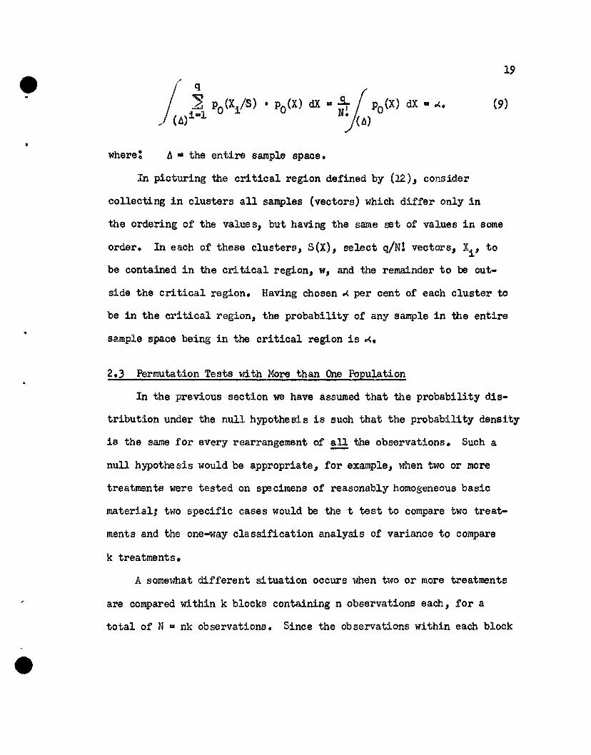
where: f:. • the entire sample space.

19

In picturing the critical region defined by (12), consider

collecting in clusters all samples (vectors) which differ only in

the ordering of the value s, but having the same set of values in some

order. In each of these clusters, SeX), select q/N! vectors, X., toJ.

be contained in the critical region, w, and the remainder to be out-

side the critical region. Having chosen ~ per cent of each cluster to

be in the critical region, the probability of any sample in the entire

sample space being in the critical region is ~.

2.3 Permutation Tests with More than One Population

In the previous section we have assumed that the probability dis-

tribution under the null hypothesis is such that the probability density

is the same for every rearrangement of ill the observations. Such a

null hypothesis would be appropriate, for example, when tl-lO or more

treatments were tested on specimens of reasonably homogeneous basic

materialr two specific cases would be the t test to compare two treat-

ments and the one-way classification analysis of variance to compare

k treatments.

A somewhat different situation occurs when two or more treatments

are compared within k blocks containing n observations each, for a

total of N = nk observations. Since the observations within each block

(10)

•20

are presumed more homogeneous than observations not in the same block,

the probability density under the null hypothesis is not the sane for

all N observations, because a different block parameter occurs in each

of the k groups. In such a case it would be appropriate to assume

that only rearrangement within a block would leave the null pro~ability

density unchangedo

Provided therefore, that each rearrangement within each block has

the sang prob3.bility density, we could again construct a region" w, of

size"" by arrc::..r,ging that q out of the (n~)k v1ithin,~block permutations

of the N observations are contained in w, with q =",,(n!)\ The type I

error may then be danoted by the N-fold integral analogous to (9)

1, k q kn PO. (X).· ~ n PO' (Xi/S) dX =""

(l~) j=l J 1 j=l J

In this and the previous type of permutation ~est discussed in

section 2 0 2, if q is not an integer, we can of course obtain a test at

approximately the desired significance level by taking the n1:o...mber of

arrangements includ3d in the critical region to be the n~arest ~nteger

to q. E~uations (9) and (10) are essentially of the same form and we

include both types of test in the discussion which follows.

Now we need make no assumption about the form of Jjhe distribution

(11)

for same set, Xl' X2' ••• , XA' of rearrangements of the sample} X.

•2.1

(where A • number of permissible rearrangements of the sample) That is

to say that samples containing the same observations will have the

same probability density for several orderings of the observations.

This would inclUde" for example, all hypotheses of the form

(12)

i.e. each observation is distributed independently with the same

density function" whatever its form. It would also inclUde" for

example" the hypothesis that the observations were distributed multi-

normally and were all equally correlated. It would" on the other hand,

exclude the hypothesis that the observations were serially correlated.

2.4 Form of Permutation Test to be Used

By using a permutation test" then" we can satiety exactly Neyman

and Pearson's first condition without seriously restrictive assumptions.

We now consider the second condition that the critioal region, w,

should be chosen such that the chance of accepting the alternative" Hl ,

when it is true" shall be as large as possible.

As was originally pointed out by E. S. Pearson (1937), by using

the permutation test the probability of rejeotion of the null hypothesis

when it is true will be maintained at the desired level".,(. However,

the probability of rejection of the null hypothesis, when the alter­

native hypothesis is true, and consequently the power will depend

directly on the specific form of the parent population. Since the

configuration of the critioal region" w , in the entire sample space, d,

•22

depends upon the statistic used in the permutation test, the power also

depends upon the choice of this statistic. \ve can only satisfy Neyman

and Pearson's second condition, therefore, if we are prepared to be

specific about the class of probability density functions Which we had

in mind in our alternative hypothesis, and base our method of selecti. on

of the critical region on this parametric alternative hypothesis. If

the alternative, H1

, is so specified, lehman and Stein (1949) have

shown how it is possible to select a best critical region:" For

example, suppose that the object of the permutation procedure was to

test the hypothesis that each of two samples came from the same distri­

bution against the alternatLve that they came from two different

distributions, one of which had a larger location parameter than did

the other. The assumption that the form of the alternative distri­

bution was the normal would lead to a test in Which for each sample

the q points in the critical region were those for which the largest

differences in means (in the anticipated direction) occurred. If the

distribution were assumed to be rectangular.. a more powerful test would

be based on the comparison of midranges.

In practice the statistician's feeling about the parent distri­

bution could usually best be expressed in terms of a distribution of

possibilities rather than in anyone particular possibility, This

mental, "prior distribution of distributions", might be imagined to

have some central value" but its range would" or perhaps should" make

the statistician reluctant to treat this value as if it were t~le only

23

one that could occur, especially if departure from this "cent.ral" dis-

tribution would lead to serious errors. In particular he would be re-

luctant to make the assumption of a specific parent null distribution

if it were possible to show (as it is for example with tests to compare

variances) that such an assumption could lead to serious inaccuracy in

estimating the first kind of error, or significance level~

On the other hand" if co( is fixed at the desired level by the use

of the permutation test" and being faced with the necessity for choos­

ing some specific alternative distribution (or implying such a choice

by "intuitive" selection of a criterion) it would seem natural for the

statistician to base his criterion on a statistic appropriate for what

he supposed to be the central alternative distribution. Even though

the statistician might expect this distribution seldom if ever" to be

realized exactly, he would expect that the loss of power suffered in

the long run for a series of tests on a series of varying distributions

would be smallest for such a statistic.

Using this rationale the choice in the above example between the

difference in means and the difference in midranges as the appropriate

criterion would be based on whether the statistician's mental picture

of the distribution of distributions likely to be met in practice in

this type of experiment was centered about the normal or about the

rectangular distribution. In most cases the normal distribution would

be chosen" though there could be experimental circumstances which would

lead the statistician to choose some other distribution as the central

one for experiments of a particular type; hence" this would lead to a

permutation test based on some different statistic.

e•

24

Permutation Moments-Suppose we have selected some criterion, g(X)" of the N observati"')~-".s

in our experiment, then for any given sample a permutation distribution

of g(X) generated by all permissible rearrangements of the obser1iaticns

is obtained and the htth permutation moment of this distribution is

given by

where the summation is over all permissible arrangements and 'toD uld in-

clude both the test situation of section 2.2 and that of section 2.3.

2.6 Overall Moments from Permutation Moments

The usual "overall" hth moment for the statistic or function g(X),

is given by

~ • E rgh(X)J(ll) -

By use of (6)" this may be written as

where: II is entire sample space.

Substituting (13) in (15), we may write

~ .. E [~J( ll)

(14)

(15)

(16)

Thus" as was originally indicated by Welch (1937)" the overall moments

may be evaluated by taking expectations of the permutation moments.

e. 2.7 Example of a Permutation Test

At this point it may be helpful to study a particular example of

the permutation test. Suppose that an experiment has been carried out

in which k pairs of observations have been made. One observation within

each pair has been made with treatment A applied and one with treatment

B. Apart from application of the treatment" conditions have baen kept as

uniform as possible within each pair but differences in average level

may occur from pair to pair. These data may be denoted by

Table 1

Example of A Permutation Test.

Block Treatments Treatment

A B Differences (

1 Xu x12 Yl

2~l x22 Y2

0 • • 0

0 • 0 •• • • •k xkl xk2 Yk

means x.l x 412y•

A-B)

This is the familiar situation encountered in the "paired obser-

vation" t test. It can equivalantly be regarded as an example of a

randomized block design having k blocks and n =2 treatments with a

total of (kn • N) observations. The null hypothesis is that discussed

26

in section 2.3, that within eaoh pair the probability density is un-

ohanged by interohanging the observations. If the alternative hypo-

thesis were that

(17)

where: IJ.. mean of all the observations

~j = treatment effeot, a constant (j =I, 2)

~i • block constants (i = I, 2, "0' k)2Sij =normal (0, a ) independent random variable

then Lehman and Stein (1949) show that the best critical region is that

based on the difference, between the sample means, x 1 M X 2 • Y , re-t e ,

ferred to the distribution generated by all permissible permutations

of the N observations, ie, all possible rearrangements ~thin blocks,

This is equivalent to basing the test on the mean of the k difference,

Yl , Y2' '00, Yk, where the observed mean differenoes is referred to the

2k mean differences generated by associating all possible combinations

of plus and minus signs with the k differenoes, 1i. This is the form

of the test as originally suggested by R. A. Fisher (1935).

As a specific example suppose that in a particular experiment in

which there were k =10 pairs of numbers, the absolute treatment dif­

ferences (the differenoes without regard to sign) were 1, 2, 3, 4, 5,

6, 7, 8, 9, 10. Then there are 210 • 1024 possible ways in which we

can attach a positive or negative sign to these numbers and oonsequently

210 ualues f th Th 1 ...~t t th t tiv 0 e mean, y. ese va ues cons~ u e e permu a on•

distribut1:on of y and this is shown for the present example in Figure 1••

• Frequency.

40

Figure 1

Permutation Distribution of The Sample Mean27

•

•

32

24

16

8

o

-

11111111 III/ /III f

o

Figure 2

Permutation Distribution

of

Frequency.

400 _

320 _

240

160 _

80 _

o

The Statistic, W

r--­..--

r--r--;-'.r--

i I I Io .1 . i/2. ..3 .. .4.

w

.7 .8 1

e.

..

28

Suppose 6 is the true difference in the means of the populations,

then to test the null hypothesis

against the alternative

at the significance level, ~ =$0/1024, we would include in the critical

region those samples that give values of;'y / ».7, since this inequa-•

lity is true for the 50 most extreme values lying outside the arrows in

the distribution in Figure 1. Alternatively, the region, y ».7,•

would supply the critical region at the level of significance,

.,0( • 2,/1024, when testing against the alternative

It will be noted that the same critical region would be obtained

had we calculated the permutation distribution for the t statistic it-

self because

Yt = ------...........----

Equivalently, if we were testing the double-sided alternative

(18)

hypothesis, we could have used the corresponding analysis of variance

criterion,

ky2F • t

2• ----,---(S-~) / (k-l),

2

(20)

• (21)

'"

where: St· trea.tment sum of squares

Se • error sum of squares

Alternatively we could have used the oriterion

~ 12 _ ky2• ----...;,=--- (22 )

which may be written as

w. 11 + (k-l)t2

which is a monotonic decreasing function of t 2,

(23)

For thi s example1 using equation

385 - 1012

w. --_.....::.-.38S

(22)1

The permutation distribution of Wcan be o~culated tram that of

y and is shown in Figure 2,,

e.

•

30

2.6 Approximation to the Permutation Test

Evaluation of the permutation distribution, or of such part of it

as is necessary to determine the critical value of the statistic~ using

the procedure above is laborious. To make the permutation theory of

practical value, use is made of the apprOXimation to the permutation

distribution based on the evaluation of its moments by the method pro­

posed by Pitman (19361 1937) and bywe10h (1937 1 1936).

let us consider the particular test considered above. Of the

several statistics demonstrated above, we shall derive the moments of

the criterion, W, because expectations of a ratio are not required in

this case due to the constant denominator over the permutation distri-

bution. Using the Wstatistic we have for its moments with respect to

the permutation distribution

I k-l (24)Ml (W) • k

[1 - JIv~ (~v). 2 (k-l)

(b2-3(2,)

k2 (k+2) k-1

The corresponding moments assuming normality are

E (W) IIk-l (26)

N k

V (W) II2(k-l) (21)

N ~ (k+2)

It will be noted that the first moment ot the permutation distribution

is the same as that for the distribution based on the assumption of

normality, while the variance of W in the permutation distribution

e.31

differs from that of the distribution based on normal theory in a term

-1ot order k ,involving the sample value of the fourth moment ratio,

(k+2) ~.}

(,>_:/>2(28)

It will be recalled that for normal theory, W follows a Beta dis­

tribution, the oumulative distribution of which may be written

(29)

where Karl fearsonls notation for the incomplete Beta ratio is

The moments of the latter distribution are mown to be

E(t) • ~' • ~p--­1 p + q

Vet) • ~ • --pq~-­(p+q)2 (p+q+l)

,Solving these in order to express p and q in terms of ~ and ~, we

(.30)

(.31)

(32)

.:

obtain

p •

q-

, , , 2~ (~1 - "1.. • ~)

~

I(1 - ~l ) P

t~l

(33)

(4)

e.32

The permutation distribution of Wis of oourse discontinuous •

However, its values lie between 0 and 1 and Pitman (1937) has shown

that its third and fourth moments agree reasonably closely with those

of a Beta distribution. It is therefore reasonable to approximate

the permutation distribution by a Beta distribution, equating the

first two moments of the two distributions. These are given in (24)

and (2$) for the permutation distribution and in (26) and (27) for

the normal distribution.

This procedure will in general have the effect of changing the

parameters, p and q, in the approximating distribution from their

normal theory values of (k - 1)/2 and 1/2, However, since from (J4)1 - ~'

q/p • 1 and from (24) and (26) the mean of Wis the same tor the~,

permutatitn distribution as for the normal-theory distribution, it

follows that both parameters, p and q, will be changed by the same

tactor. We will denote this tactor by the symbol, do

Thus we may write the type I error of the approximate permutation

test in the form

where the modifying constant

(k + 2)(b2 - 3)d • 1 + ----.;;.--

k(k + 2 .. b2 )

b2 .. 3• 1 + --------

k [1 .. b2 ]k + 2

(J6)

e.JJ

or approximately for large k

b - Jd :I 1 + ....2 _

k(31)

We can now transfom OS) back to the F fom. Thus" finally \ole

have that, as an approximation for the permutation test" we should

perform the usual F test but instead of employing 1 and k - 1 degrees

of freedom. In the example discussed above we find that with the

observed values of the absolute treatment differences" 1" 2, ... , 10,

and with the oritical region, w, defined by / Y / > 3.1, the error of•

the first kind for the permutation test is 4~88 per cent. Using the

approximation to the permutation test, we get 4.95 per cent as opposed

to the normal theory value of 41152 per cent.

2~9 The Critical Region for the Approximate Permutation Test

It will be noted that we have defined our test procedure for the

approximate permutation test and hence the critical region, w, in

terms of whether or not the inequality

(38)

is satisfied, where F~(b2) refers to the ~ percentile point of the F

table with degrees of freedom modified by the factor" d" W1 ich depends

upon the sample value of b2 • This is in contrast ldth the more con­

ventional test whioh defines the critioal region" w, as those values

whioh satisfy the inequality

F > F~

e..34

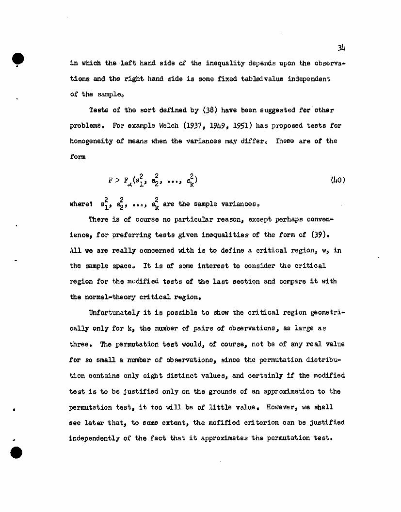
in which the ·left hand side of the inequality depends ulJon the observa­

tions and the right hand side is some fixed tablErl value independent

of the samp1eo

Teste of the sort defined by (38) have been suggested fQr other

problems. For example Welch (1937, 1949, 1951) has proposed tests for

homogeneity of means when the variances may differo These are ot the

fom

222where I 61, s2' Of> 0, sk are the sample varianceso

There is of course no particular reason, except perhaps conven­

ience, for preferring tests given inequalities of the form of (39)0

All we are really concerned with is to define a critical region" w, in

the sample space" It is of some interest to consider the critical

region for the modified tests of the last section and compare it with

the normal-theory critical region.

Unfortunately it is possible to show the cr! tical region geometri-

cally only for k.. the number of pairs of observations, as large as

three. The permutation test would, of course.. not be of any real value

for so small a number of observations, since the permutation distribu-

tion contains only eight distinct values, and certainly 1f the modified

test is to be justified only on the grounds of an approximation to the

permutation test, it too will be of little value. However.. we shall

see later that.. to some extent, the mofif'ied cr! terion can be justified

independently of the fact that it approximates the permutation test.

35

The critical region of any test independent of scale must neces­

sarily be conical (since a set of observations, Yl' Y2, ... 0' Yk has the

same significance as a set'(~l' ~2' ••• , A1k>. Both the normal­

theory test and the approximate permutation test are of this type and

their critical regions for k • 3 are shown in Figures 3a and 3ba

Figu:"e 3a. is a sketch of the three dimensional sample space. In

Figure 3b a section of the critical region in the plane, Yl + )"2+ "3-10

is shown in greater detail. By including the scales of Y'l' Y'2' and Y'3'

we have a diagram in trilinear coordinates and we can see at a glance

which types of samples are included in w by each of the two tests.

It can be seen that the approxima te permutation test differs

from the normal-theory test chiefly in selecting as significant samples,

those samples which are found non significant by the standard t test

beoau~ an outlier increases the variance 1I To take a hypothetical

example with more observations, suppose that we have ten differences,

nine of which are equal to +1 and the remaining one to +11. Then we

find that t = 2,0 and entering the usual table s with one and nine

degrees of freedom, the corresponding probability is .0766.

Using the modified test, we find that b2 • 10a402 and d • 6.,88;

thus we should enter the tables with 6.6 and 59 degrees of freedom,

which gives the corresponding probability of .00190. The exact

randomization test WOUld, of course, give a value of 1/512 = .00195,

since this sample and the corresponding sample in which all the

differences are negative are the most extreme possibilities out of

the 1024.

e..

..

Figure 3(a)

Normal",Theoryand

Approximate-Permutation

Critical Regions

36

37

Figure 3(b)

7

o 10

6

Y3

.' ·5•

.. --.• •• • fl·.... ' '4,.,..... " . ... ." .'" ... .. ...

3

Yl 2

1

010

Critical Region, lJ. 10 .

Comparison of Normal-Theory

And Approximate-Permutation•

e•

38

2.10 Use of the Permutation Test to Estimate the Approximate Effect

of Non Normality:

We shall use the example of the test on paired observations dis-

cussed above to illustrate one further application of the permutation

approach.

We have seen in section 2.7 that it is possible to derive the

overall h1th moment of a function of the observations, g(X), by con-

sidering first the permutation moments of the function and then taking

expectation of these permutation moments over all possible samples.

For example" from (22)" we have the criterion

•

sW. e_

Se .... St

whose exact moments with respect to a general" non-normal" parent

population of XIs are

E(W) • 11k

(41)

(42)

Where:

(43)

b2 = (k + 2) --­(~y2)2

In particular when the distribution is normal

e•39

and we obtain the normal moments given by (26) and (27) •

When E(b2 ) " 3 we can as an approximation fit a beta distribution

to the distribution of Wand we have for the approximate probability

when the distribution is not normal

Where the expression for 6 is the same as for d except with b2

replaced by E(b2). That is

E(b2) • 3

6· 1•k[1 •-:(.....;....nor approximately if k is large

E(b2 ) - 36·1+-......-­

k

(48)

(4S)

(46)

As before we may now change the Be ~a function back to the F form and

the approximate distribution under non normality of the statistic, t 2,

is given by the F distribution with 6 and 6(k - 1) degrees of freedom.

Since b2 is in the form of a ratio t it is necessary to expand

the denomina~or in a power series in a manner similar to that employed

by Pearson (1931) and several other writers. Using this technique,

. -1we obta1n to order k

(47)

e..40

may be estimated for various values of k and ~2' Table 2 shows a few

Table 2

Type I Error for Paired t Test

Nominal .,( • .0$

k ~~ (j2

2 3 4

9 0 .0$$2 .0$00 .0492

1 .0$$2 .0$00 .0$71

1.$ .0540 .0469 .0492

21 0 .0512 .0500 .0486

1 .0$12 .0500 .0498

1.5 .0518 .0496 .0486

41 0 .0$08 .0500 .0493

1 .0508 .0500 .0495

1.$ ,,0508 .0500 00493

e•

,

41

It should be noted that no value has been designated for the

value of ~4' For practical purposes, forms of frequency functions are

usually designated by the first four moments" though this characteri-

zation is not unique. Various classes of distribution functions may

be used when fitting by moments, two of which seem to suggest them­

selves most readily for this situation.

The one assumption that could be made in this case would be to

say that deviations from normality will be assumed to occur in the

first four moments" while the sixth moment will be given its normal

theory value" ~4 III 15. A second assumption would be that the fitted

curve was of the Pearson type, which defines the fifth and higher

moments as a function of the first four moments. Throughout this

investigation we have used the latter convention~

2 011 Summary

In this chapter we have utilized the fact that the permutation

test may be used to perform two useful functions.

1. It may be used to give a modified test procedure which will

in effect compensate for departures from assumptions. This

is effected by calculating a factor, d, a statistic used to

modify the normal-theory degrees of freedom.

2.. It can be used to provide approximate estimates of the effect

of departures from assumptions of standard normal-theory tests.

This is effected by calculating a factor, 8, a parameter used

to modify the normal-theory degrees of freedom.

e• We shall now consider these applications in more detail. In

Chapter III modified t tests and analysis of variance tests based on

the permutation moments of Pitman (19.37) and Welch (19.37, 19.38) are

indicated. In Chapter IV the approximate effects of departures from

42

,

assumptions, using the procedures mentioned in section 2.10, are

indicated. In Chapters V and VI these methods are applied to provide

a robust test to compare variances.

e• Chapter III

MODIFIED t TESTS AND ANALYSIS OF VARIANCE

Using the methods described in seotion 208, approximate permu-

tation tests have been derived for several tests comparing means. As

indicated, these tests all have a critioal region of the form

where~ d = a sIDnple estimate of a measure of non normality or

varianoe heterogeneity.

(47)

Therefore the test is uniquely defined by stating the formula for

the modifying faotor, d, as a funotion of the observed sample. These

are given belowo

3.1 Randomized Blocks

where~

d =1 + (ke - k + 2)v2 .. 2kk(s • l)(k • V2 )

k

~ (k2i • k2 )2_2 i=l 0

V- CI ;;;...-----:----

(k • l)k~\l

v =sample coeffioient of variation of block variances

~i IS sample variance in the i' th blook

s D number of treatments

k = number of blocks

(48)

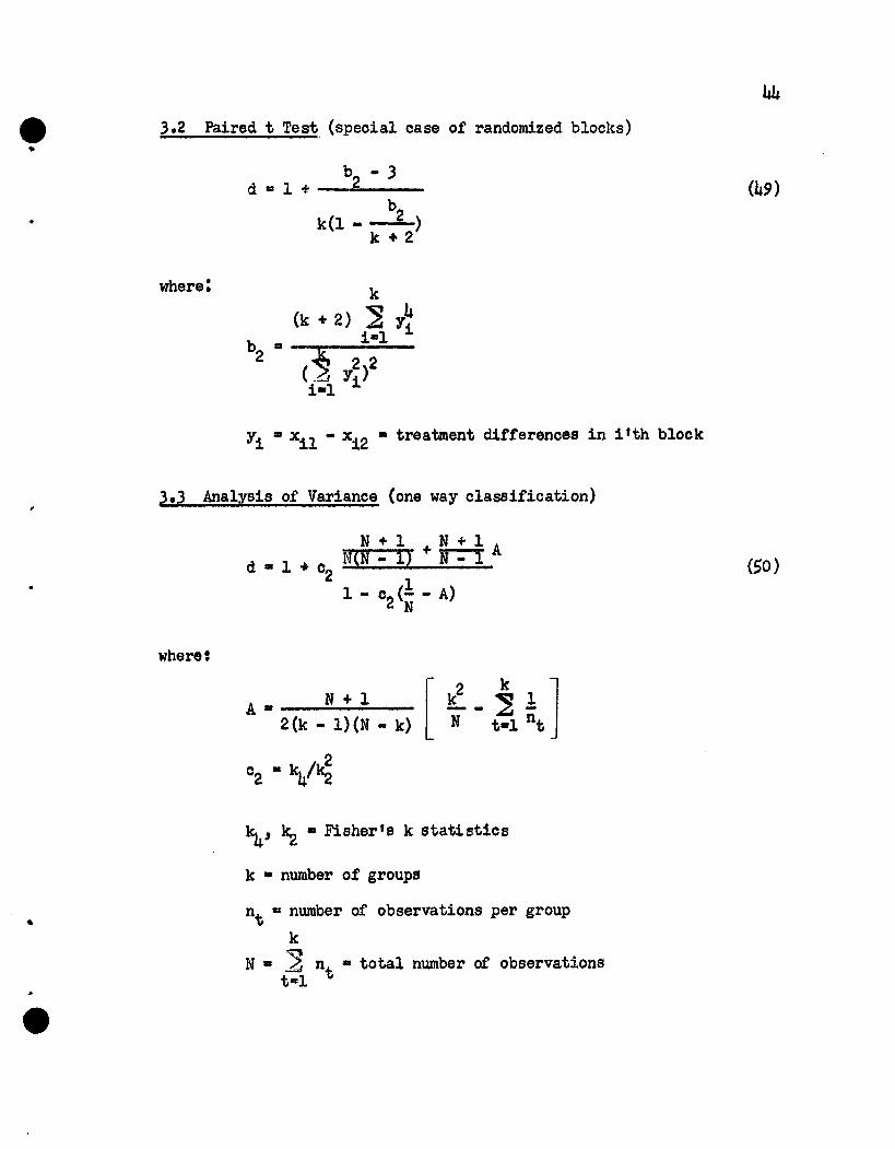
3.2 Paired t Test (speoial oase of randomized blooks)

b - 3d. 1 + _~2 _

bk(l _ 2)

k + 2

44

(49)

where:

Yi • xil - xi2 • treatment differenoes in i'th blook

3.3 Analysis of Varianoe (one way olassifioation)

N + 1 N + 1N(N - 1) + N - 1 A

11 - 02 (N - A)

wheret

(So)

A • N + 12(k - l)(N - k)

O2 • k4/~

\" ~ • Fisher's k statistios

k • number of groups

nt

• number of observations per group

k

N· ~ nt • total number of observationstel

45

Noting that for equal-sized groups, A • 0, the formula simplifies in

this special case to

(N + 1) 02d • 1 + -----:=----

(N - l)(N - 02)(51)

It is interesting to note that all of these tests are asympto­

tically equal to the normal-theory test, because the modifying factor,

d, always tends to unity with increasing sample size. This then con­

firms the robust nature of the normal-theory tests for these cases.

e•

Chapt.er IV

EFFECT OF NON NO&TI.1ALITY AND UNEQUAL VARrANCES ON t TESTS AND

ANALYSIS OF VARrANCE

Using the methods described in section 20 10, modified tests may

be derived for situations where the parent populations deviate in a

specified manner from the parent populations assumed in the derivatioll

of standard test,s, As indicated, these tests all have a critical

region of the form

,

(52)

where: 5 • a measure of the extent to whioh the standard assumptions

of normality and homoacedasticity fail to hold in the

postulated parent populationo

The:oefore the test is uniquely determined by the fO!'Illula for the

modifying factor 3 5, as a function of the type of parent populationo

A factor~ 53 near unity indicates that the standard test is very

near1¥ like the approximate permutation test, and therefore quite

robust with respect to the failure of the standard assumptions con-

sideredo A value of 5 not near unity should warn the experimenter

against the use of the standard test if it is expected that the

assumptions will fail in the manner postulated, Then the use of a

more robust test is suggested; for some situations these are given in

Chapter III.

• 4.1 Formulae for 5.

4.1.1 Randomized Blocks

Effect of Non-Normality:

ks(s - 2) ~6 • 1 + ----------.;;;..-.----

ks(s • l)/-ks - k .. 2 7 + k(s - 1)2 h" - 2

41

(53)

where: k a number of blocks

B • number of treatments

~ ... Population standardized 4th curnulant ... (~2 - 3)

For very large samples,

26=1+-~

ks

Effect of Unequal Block Variances

(ks .. k + 2) E(Al ) .. (8 .. 1)6 ... 1 + ------...;;..----

k(s .. 1)(1 .. E(Al ) )

where I E(~) .!....!...!O + --!:.- 02 8--0a • 1 2 s .. 1 2 s .. 1 3

<:-1 2

O2

...~K2i

~ 2( K2i )

o a~K~i

3(] K

2i)3

K2i a ai a Population variance of i~ block.

(54)

(55)

eT

48

The Simultaneous Effect of Non·Normality and Unequal Block Variances

(ks - k + a) E(Al + ~) - (s - 1)5 • 1 + -------=--..;:;..----

k(s - 1)(1 - E(Al ~~) )(56)

where:

where: th thK4i

1:1 Population 4 cumulant in i block.

Note: E(Al ) represents the effect of inequality of

variance, while E(~) represents primarily the

effect of non-normality.

4.1.2 Analysis of Variance (One-way classification)

Effect of Non-Normality

1 + 2N E(C2)5 III -------:.-

1 • ,- ~ - u.7 E(C2)

(57)

where: k 1:1 number of groups

nt • number of observations per group

e1

49k

N· .2 nt • total number of observationstal

u • N

2 (k - l){N - k)

K + 2A = ...r __r (r + 2)

K2

2

For equal sized groups the factor" U" is zero and the formula simpli­

fies to

•

6. 1 _

1 - i E(C2 )

N------N - E(C2)

Since it is desired to tabulate the effect of non-normality in

terms of the third and fourth cumulants or moments" there is no unique

value which can be assigned to the sixth cumulant occuring in the

expression for E(C2). Two reasonable approaches suggest themselves.

The sixth cumulant may be given its normal value, 0, for all cases" or

the fitted distribution may be restricted to the set of Pearson curves"

in which case the sixth cumulant is a known function of the third and

fourth cumulants. tie shall adopt the latter convention.

The same problem arises in t test for paired treatments and the F

test for comparing two variances. Here again the convention of using

the Pearson system to determine the sixth moment will be used. This

e.,

50

formula is

where '

~ • 5/.- ~ ~3 • (1 .. ~ .t.) ~2_74 1.1.,.

2

2~2 - 3~1 - 6.,(.. - ....._-----

~2 + 3

(58)

4.1.3 t Test for Comparing Two Means

The simple t test for comparing two means would be handled by

one of the two preceding formulae) depending upon whether it has

equal or unequal numbers of observations in the two treatments.

4.104 t Test for Paired Treatments (randomized blocks with 2

treatments)

where:

b2 and ~2 • sample and population fourth etandardized

moments respectively of the differences between

the two observations in each block.

4.1.5 F Test far COmparing Two Variances, with Means Known

6 .[~ + ~1E(°

2) • II ; 1J - ~ (60)

e, where: N = total number of observations

51

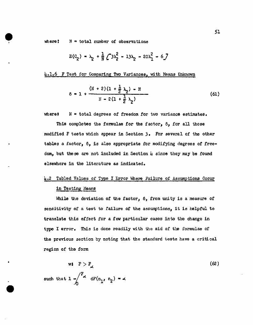
4e l.6 F Test for Comparing Two Variances, with Means Unknown

6 • 1 +(N + 2)(1 + ~ ~) - N

I~ - 2 (1 + i A2)(61)

where' N • total degrees of freedom for two variance estimates.

This completes the fomulae for the factor, 6, for all those

modified F tests which appear in Section 3. For several of the other

tables a factor, 6, is also appropriate for modifying degrees of free­

dom, but these are not included in Section 4 since they may be found

elsewhere in the literature as indicatedG

402 Tabled Values of Type I Error Where Failure of Assumptions Occur

in Testing 111eans

While the deviation of the factor, 6, from unity is a measure of

sensitivity of a test to failure of the assumptions, it is helpful to

translate this effect for a few particular cases into the change in

type I error. This is done readily wi. th the aid of the formulae of

the previous section by noting that the standard tests have a critical

region of the form

wI F> F.(

such that 1 iF.. dF(n1

, "2) ...

(62)

e.. Since F is not distributed as F{~l' n2), but rather as F{5~1' 5n2),

the actual type I error when using the standard test is not .(, but

rather

_/F.(a • 1/0 dF(6nl " 6~) (63)

With this use of the approximate pe.::'ml~tation test" several tables

have been prepared" giving the actual type I error when the standard

test is applied in situations where specified deviations from the

assumptions oocur. ~fuerever possible ex~erpts have been taken from

tables pUblished elsewhere to give a more complete picture of the

effects of failure of assumptions in a broad class of problems. In

these cases, the approximate permutation theory does not permit

evaluating these errors.

Two types of designs for comparing two or more means will be con-

sidered in this section, randomized blccks and the one-way classifi-

cation analysis of variance. The effect of non-normality will be

considered for both, and the effect of inequality of varian ces will be

considered for the first ot these. Also student's t test for comparing

a sample mean with a hypothesized value will be considered.

402.1 Randomized Blocks - Inequality of Block Variances

Exact values for the type I error in randomized blocks with

unequal block variances are taken from Box (1951) and given below.

These are compared with values obtained by the approximate-permutation

test theory.

53

Table 3

Comparison of Exact and Approximate-Permutation Type I Error

for Randomized Blocks with Unequal Block Variances

Nominal .( IS .05

No. of No. ofTreatments Blocks Block Variances Exact Approx.

(6) (k) (~i) .,( .,(

i 11 3 1, 2" 3 .0425 .0436

ii 5 3 1, 2, 3 ,0427 .0426

iii 11 3 1" 1, 3 .0376 .0388

iv 5 3 1, 1, 3 .0391 .0411

v 3 5 1, 1, 1, 1, 3 .0447 .0413

vi 3 11 1, 1, ... , 1, 3 .0486 .0478

4.2.2 Randomized Blocks - Inequality of Treatment Variances

Approximate type I errors for randomized blocks with unequal

variances in the treatments are taken from Box (1951) and given below.

Permutation theory does not give an approximation for this situation.

e\ Table 4

Type I Error for Randomized Blocks with Unequal

Treatment Variances - Nominal ~ = ,05

No. of No. of Treatment 'l'ype IBlocks Treatments Varia..l1c€:s Error

(k) (s) (K2i ) (,.()

i 11 3 1, 2, .3 .0549

ii 5 .3 1, 2, .3 .0559

iii 11 .3 1, 1, .3 ,0,93

iv 5 3 1, 1, .3 .0612

v 3 5 1, 1, 1, 1, .3 .0692

vi .3 11 1, 1, "0, 1" 3 .0109

4.2 f .3 Randomized Blocks - Non Normality

Permutation theory permits obtaining the following approximate

values for the type I errore

54

e "Table ,I

Type I Error for Randomized Blocks with Non-

Normal Parent Population - Nominal P( .. .0,

No. of No. of Population Fourth Cumulant (A2

)Blocks Treatments

(k) (s) -10' ..1,0 -0 0 , 100 2.0 2"2. , .077, .064, .0,6, .0408 .0340 .0320

2. 10 .0,92 .0,,6 .0,27 .04" ,0418 .0400

2 21 .0,3, .0,23 .0,11 .0477 .0460 ..04,1

2 41 .0,16 .0,11 .0,06 .0490 .0479 .0474

5 , .0,,2 .0,33 .0,16 .0470 110447 .0436

4 21 .0,14 .0,10 .0,0, .0490 ,0481 .0471

11 , .0,18 .0,12 .0,06 .0488 .0476 .0472

4.2,4 Paired t Test (Special case of randomized blocks)-Since there is only one degree of freedom for error within each

block, under the null hypothesis, it is not possible to separate the

effect of non normality and inequality of block variances in the case

of the paired t test. Therefore it will be convenient to consider

these two failures of the assumptions by non-normal third and fourth

moments of the variable, y, the differences between the treatment

yields within each block.

• Although these figures were given in Table 2 of section 2.10,

they will be repeated here for completeness of this section.

56

e Table 6\

Type I Error for Paired t Test

Nomina1..t. .. .05

k ~2~21

2. 3 h

9 0 00552 .0500 .0492

1 Q0552 .0500 .0571

1.5 e0540 00469 .0492

21 0 (/0512 .0500 .0486

1 110512 .0500 ~0498

1.5 ~0518 .0496 .0486

41 0 .0508 .0500 .0493

1 G0508 00500 .0495

1~5 .0508 aO,OO 110493

4 0 205 Analysis of Variance (one-way classification) Effect of

Non Normality

The effect of non normality on the analysis of variance for the

comparison of k means was evaluated by Gayen (1950b) by the use of the

Gram Charlier series to represent the parent populations. Selected

values from his table are compared with results obtained by the

simpler method of the approximate permutation test. Both results are

given below,

e•

Table 7

Type I Error for Comparing k Means in The Analysis

of Variance (with 5 observations for each of 5 treatments)

Non Normal Parent Populations - Nominal ~ III .05

57

-1.0

o

0.00

.0524 .0529 .0534

( .0524) ( .0521) ( 00516)

.0500 .0505 .0510 .0515

(.0500) (.0500) (.0491) (.0482)

.0452 c0451 .0462 .0461

(.0568) (.0528) ( .0468)

Note: upper values from Gayen" lower values permutation

theory

4~2.6 Analy!isof Variance (one-way classification)

Effect of Inequality of Variances

From Box (1951) we have taken a few values to indicate the

effect of inequality of variances within groups for situations where

the groups are equal and unequal. It should be noted that with equal

groups the test ShOlvS the robustness which has been found in the

p,,'svJ OU8 tests, hut. that. when a large. or small variance occurs in a

e•

58

group which has a very small percentage of the total observations,

the effect of heteroscedasticity is quite severe.

Table 8

Type I Error for Comparing Three Means in The Analysis of Variance

Effect of Heterogeneous Error Variance • Nominal .,.( • .os

Group Variances Number at Observations Totel .,(

in Each Group N

2 2 20'1 0'2 0'3 n1 n2 n

3

1 1 1 5 5 5 15 .0587

1 1 3 7 5 3 15 .1070

1 1 3 9 5 1 15 .1741

1 1 3 1 5 9 15 .0131

4.2.7 t Test for Comparing Two Treatments

Effect of Non Normality

By use of permutation theory we may obtain the approximate effect

of non normality on the t test.

e 59

Table 9~

Type I Error for Comparing Two Means Non-

Normal Parent Populations" Nominal co< • .05

No. of "A2

A.21

Blocks 0 1 1.5

5 -1 .0562 .0493 .0438

0 .0500 ,0425 .0358

2 .0737 .0598

11 -1 .0534 .0520 .0510

0 .0500 .0485 .0471

2 .0555 .0492

21 ...1 .0518 .0515 .0512

0 00500 .0496 .0492

2 .0496 .0478

-~.2.8 Testing a Mean Against A Hypothesized Value (Student.s t Test)

While it is not possible to estimate the effect of non normality

on the t test in the case of te sting a value of the sample mean

against a hypothesized value of the mean by the permutation-theory

method, Geary (1936) has estimated the effect of non normality for

samples of 10.

Table 10

Type I Error for One Sided t Test Sample

Size • 10 Nominal ~ = 0025

Ai A2 Type IError

0" 1 .024

1/2 0 ,041

1 0 0072

1 1 ,086

Here again there is insensitivity to the population fourth moment,

but in contrast to tests for comparing two or more means, rather

small deviations of the third cumu1ant from zero cause an appre-

ciab1e change in probability.

4e3 Summary of Tests for Means

From the foregoing tables it can be seen that a large variety of

tests for comparing means are highly robust to both non normality and

inequality of variances. Therefore the practical experimenter may use

these tests of significance with relatively little worry concerning the

failure or these assumptions to hold exactly in experimental situata-

tiona. The rather striking exception to this rule is the sensitivity

of the analysis of variance to variance heterogeneity when the groups

are of unequal size.

61

Studentts t test for testing a sample mean against a hypothesized

value l in contrast to the tests for comparing two or more means" is

quite sensitive to skewness in the parent population.

e•

62

Chapter V

TESTS ON VARIANCES.. MEANS ASSUMED KNCMN

Since it has been demonstrated that tests for comparing variances

are extremely sensitive to non normality, an approximate permutation

test will be derived by the method of fitting a Beta distribution to

the first two permutation moments as outlined in section 2.8.

5.1 Test to Compare Two Variances, Means Known

The simplest case in which a test may be made for equality of

variances is that of two groups with the mean of each group known.

There is no loss of generality in assuming that the two known means

are zero. The statistic most commonly used to test this hypothesis isn

:1 r./nlF a ial 1 (64)

n

~ Y~/~j=l J

where: Xi. the i-th observation o£ the first sample

Yj • the j-th observation of the second sample

An equivalent statistic for testing this same hypothesis is

n1

~ X2

i=l iW a --.;;.,..;;;....---

~ ~

~l Xi+ j~l Y~

(6)

eII

63

Since this statistic is an exact equivalent of the more common F, and

lends itself to simpler algebraic rnanipu1a tion, the theoretical deve!-'

lopment will be concerned with the distribution of W. As 1'1 is distri-

buted as a Beta variate for samples drawn from a normal population, its

first two moments are

( t6)

(61)

where vl ' V2 a degrees of freedom

The moments of Wwith respect to the permutation distribution are

where:

If these moments of the permutation distribution of Ware equated

to the corresponding normal moments, the following relationship is

found:

e•

64

(70)

where:

2--N (7).)

Since there is a one to one correspondence between the Wstatistics

here investigated and the F statistic used to test the same hypothesis,

this result suggests that the appropriate statistic is

(72)

rather than the conventional

(13)

That is, the appropriate statistic is the conventional F with degrees

of freedom modified by the sample fourth moment as indicatede

There are however two questions concerning the F approximation to

the permutation test.

1. How good is the moment app!'oximation to the permutation test?

2. It is well known that when the parent distribution is normal,

the standard F test is uniformly most powerfulo Therefore it

is of interest to estimate how much power is lost if the parent

distribution is normal by using the modified test in ord~r to

obtain the property of robustness.

65-

In order to answer these two questions a rather extensive empirical

sampling experiment has been performed.

5.,2 Sampling Experiment to Study Two Procedures for Comparing Two

Varianoes

In order to study the power function and robustness of the

standard F test and the modified F test, the power functions and the

null distributions of these statistics were investigated for the

rectangular, normal and truncated double-exponential parent distribu-

tions.

The empirical sampling procedure involved drawing 2000 samples of

size 20 from each of the three populations~ These were paired to give

1000 values of the standard F and the modified F for each population.

The appropriate probability associated with each of these FC s was

estimated from a set of graphs prepared from Pearson's "Tables of The

Incomplete Beta Function". These probabilities for the two statistics

and three distributions are summarized on Figures 4, 5 and 6.

In addition to the calculations above, which evaluate the

behavior of these statistics When the null hypothesis is true, the

distributions of these statistics were estimated far three alternatives

to the null case:

2 220'1 • 02

2 2401 • 02

2 2001 lit 02

e•

•

66

In order to decrease the amount of IBM calculationl a dodge

was used in drawing the original 40,000 samples. For each of the

three populations" one hundred values of the ordinate of the density

functions were calculated at the 0.5, 1.5, 2,5, •••, 99.5 percentile

points. The squares l cubes and fourth powers of each of these

ordinates were calculated on a desk calculator l and all four of these

quantities were punched on one IBM card for each of the one hundred

percentile points and for the three distributions I making a master

deck of 100 cards for each distribution.

The sampling deck of 40,000 cards was then made up by putting

on blank cards a two digit random number, and a sequence number running

from one to 4°1000. ~hese were then sorted into 100 groups according

to the random number appearing on the card, On each card containing

random number 00 was punched the 0,5 percentile value of the variate

with its square" cube and fourth power; on the card with random number

01 was punched the 1.5 percentile value, etc. The 40,000 cards were

then sorted into their original sequence by the sequence number to give

the sampling deck from which 2,000 samples of 20 were drawn.

Before analyzing the results of this experiment it is instruc-

tive to note the imperfection in the three populations due to this

truncation caused by selecting only one hundred values to approximate

continuous distributions. Comparisons of the theoretical and actual

fourth moments l ~2' are shown below.

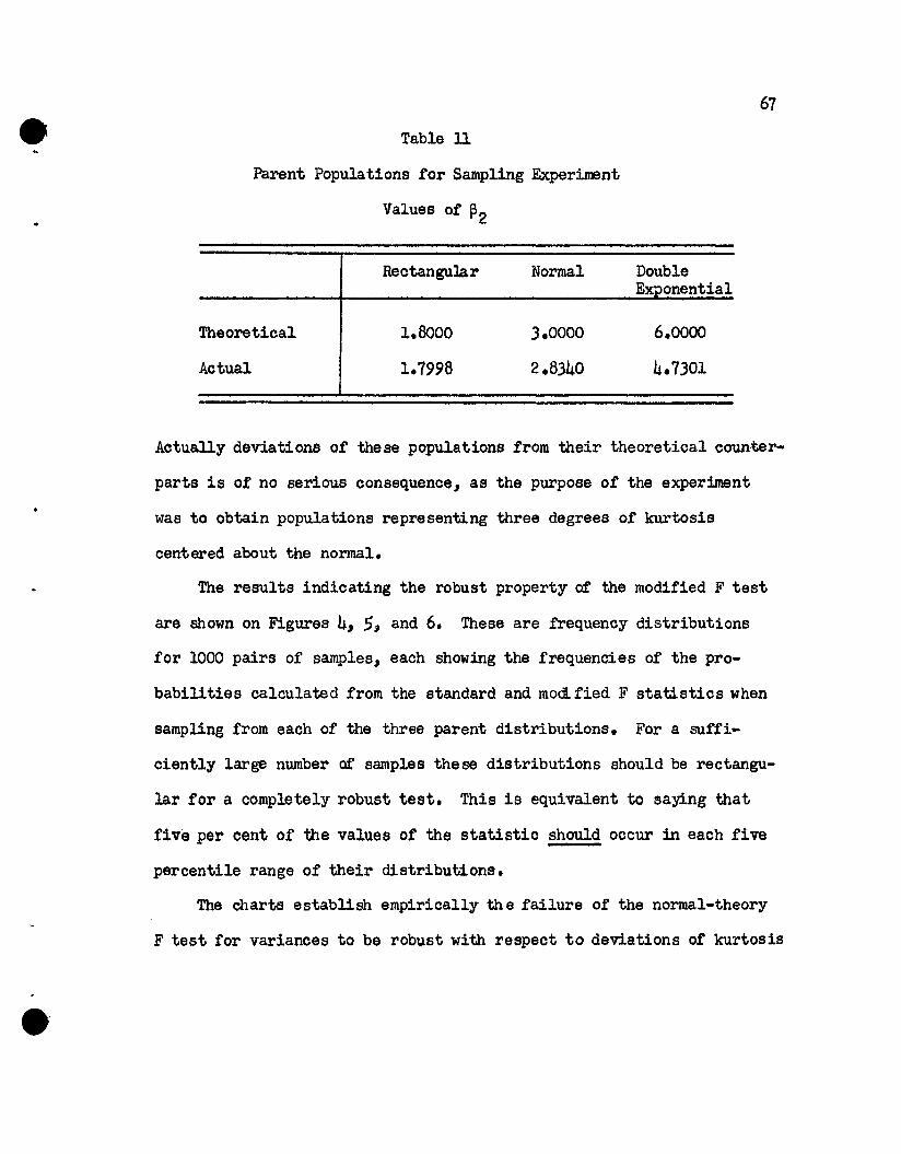
67

e Table 11

Parent Populations for Sampling Experiment

Values of ~2

Rectangular Normal DoubleEx onential

Theoretical 1.6000 3.0000 6.0000

Actual 1.7998 2.8340 4.7301

Actually deviations of these populations from their theoretical counter-

parts is of no serious consequence J as the purpose of the experiment

was to obtain populations representing three degrees of kurtosis

centered about the normal.

The results indicating the robust property or the modified F test

are shown on Figures 4, 5J and 6. These are frequency distributions

for 1000 pairs of samples, each showing the frequencies of the pro­

babilities calculated from the standard and modi. fied F statistics when

sampling from each of the three parent distributions. For a sufii-

ciently large number of samples the se distributions should be rectangu-

lar for a completely robust test. This is equivalent to saying that

five per cent of the values of the statistic should occur in each five

percentile range of their distributions.

The charts establish empirically th e failure of the normal-theory

F test for variances to be robust with respect to deviations of kurtosis

Figure 4

Rectangular Parent Population

Standard F Test90

68

Frequenc

30

75

60

45

15

o

,-

- .--

- - f--

,..- r-- ~

- l-

t---I--

-

Y I--_r--

- ....-'--

I-

h

RobustF Test

75 -

60_ -

-

45---Frequency ~

30 -

15 -

- -

o - '---- . _._- .. -.

o 5 10 20 30 40 50 60 70Nominal Percentile Groups

80 90 100

Figure 5

Normal Parent Population

Standard F Test

69

75

Frequency&J

45

30

A 15

0

- ,-

- r---

.----""-1-- ~

-~

.---- 10-'- I---r-~ I--r--- I---

-

-I-- I--

-

Robust F Test

-

.-- r- .-- ,-

.--,- r--

.--- -- I---..-- I--- I--

t---r- f--I- f--

I--

-

-

75Frequency

60

45

30

15

oo 5 10 20 30 40 50 60 70

Nominal Percentile Groups80 90 100

70

Figure 6

Double Exponential Parent Population-,...---

r--

y

-

r--- -r--- r---

-- - r---I-- -

r---f--f-- -

f-- -- I--

-

30

60

o

15

75

45

105

90Frequenc

StandardF Test

120

1009080706050403020

- -

-- -- r---f--

'--t--- - -- I--r-- -- --- 1-

-

-

oo 5 10

30

15

45

60Frequency

RobustF Test75

Nominal Percentile Groups

71

from normal. They also establish the relative robustness of the

modified F test for these same leptokurtic and platykurtic populations.

For the rectangular parent population, the standard F test shows

007 I2r cent of the values below the 5 per cent point and 0.6 per cent

of the values above the 95 per c~nt pointo The modified test corrects

almost perfectly for this lack of robustness in the standard test,

showing 4., per cent of the values below the 5 per cent point and 4.7

per cent of the values above the 95 per cent point"

For a robust test, fifty samples would be expected in each cell

of the chart. The use of chi square to compare the actual frequencies

with this ideal behavior illustrates the improvement with the modified

testlt With nineteen degrees of freedom, the value of chi square is

reduced from 254.16 to 21.84 by the modification of the F teat; this

clearly indicates that the standard F test is not behaving properly,

while the observed frequencies of the modified test are compatible

wi th the hypothesis of a robust test. The results of sampling from

all three parent populations may be summarized by the following table.

72

Table 12

Sampling Results Summary for Comparison of Standard(S) F

and Modified (M) F Teets

Parent Population Rectangular Nomal DoubleEXPonential

Standard Modified S M S M

PerCentBelow S% Point 0.7 4.$ 3.0 4.0 10.2 3~6

Per CentAbove 9$% Point 0.6 4.7 3.0 3.$ u.o 3.6

Chi Square(19 d.f.) 2.54.16 21.8 36.12 27.84 166.20 32.96

Probability ofExceeding less lessObserved than thanChi Squ~e* .001 .290 .011 0.860 0001 .02$

* Assuming HO: The test is robust with respect to the parent-

population sampled.

Having established the relative robustness of the modified test,

the question arises as to how much power is lost by the modification of

the standard test, when in fact the parent population is normal. Chart

7 shows the power curve for the standard and mOdified F test for

.( D .0$. The power curve for the standard F test agrees closely with

the theoretical po\'ler function of the te st.

From the graph it appears that there is very little loss of power

due to modifying the F test. For example, the probability of detecting

•

73

a variance ratio of 3a is reduced from about .75 to about .71 by the

use of the modified test. Since this difference in power is subject

to a sampling error of .02, the ninety-five per cent confidence limits

on the loss of power is (.00 - .08).

It is interesting to note that the power curve for the standard F

test with 18 and 18 degrees of freedom, ~ • .05, coincides almost per­

fectly with the modified F test curve for 20 and 20 degrees of free-

dome This indicates a loss of power of about ten per cent in the sense

of requiring ten per cent more observations with the modified F than

with the standard test to obtain the same power curve.

Since the standard F test does not have the proper 5 per cent

intercept for the non-normal populations, the comparison of power

curves for the two tests in these case s is of relatively less interest.

However, these are shown in Figures 8 and 9. What can be noted is that

the mOdified test is most powerful for the rectangular and least power-

ful for the double exponential. That is to say the power decreases

with increasing ~2'

5.3 Test to Compare k Variances, Means Knovm

The next simplest case of a test for the equallty of variances is

that of comparing k groups, where the mean for each group is kno~m.

Again the known means may 1::s assumed equal to zero.

The statistic most commonly used to test the equality of k vari­

ances is the Bartlett statistic; note that here the formula is slightly

modified due to the zero means of t.'le groups•

e· It Ie

Figure 7

Power Curves~*" - Normal Distribution- - -------- ---~-~ - --

0--"- _ -;.;:-.~ .-;';. ••••••••••••• rno ............. -/ •••••••• ~o- ,

/ -;:...... / 0-

/. ....-t<' ..

//,//

.//

/'/r.t.

~.

/.../..'

/0"

1.0 r'--------

.9

.8

.7

•6Power(l-~) .5

.4

.3

.2

.1

........... t

~(o

Standard F (Theoretical)

Standard F (Empirical)

Robust F (Empirical)

Nominal J.. ....05

-J,f::""

653 4Variance Ratio

2

A' I

1

e· .. • ·e

Figure 8

Pouer Curves~~ - Rectangular Distribution

1.01 --------------------- ~- ---------- o

-J\J1.

65

Nominal J.. = .05

Standard F

Robust F

-~-

3 4Variance Ratio

2

.......--'

././

/,/

/'/

//

//

//

//

//

/

cf/

//

//

//

/

//

//

//

1o n I

.3

.2

.4

.8

.6

.7

.9

Power(1-B).5

e- .. ·e

Figure 9

Power Curves'::- ... Double Exponential

.;"

6 (f..

~ -- ----.....-...,--

5

Standard F

Robust F

Nominal .I... :: • 05

,./

.-,./

~=-

,./,./

4

/cY./

/'

//

32

,,./

././

/'./,

./,,./

fl/'

/'./

/'/'

././

/'

1.0

.9

.8

.7

.6Power(1-13)

.s

.4

.3

.2

.1

01

71

where:

sample variance of group t

a average s3mple variance

nt =number observations in group t

k a number of groups

Xti =observation i in group t

k

N • ~ ntt=l

The critical region used for the statistic is

(75)

. i -1where A is a modifY1ng quant ty of order N proposed by Bartlett

(19.34). Since" however" the test depends on ~2 to order NO: there is

little point in considering this refinement, and we shall consider the

critical region defined by

(76)

Since it has been shown" Box (195.3), that this test is extremely sensi-

tive to non normality" an approximate permutation test has been derived

by fitting the first two moments" as outlined in section 2.8.

The first step in the derivation is to evaluate to order NO, the

b - 1E (M) = (k _ 1) ( 2 )P 2

permutation moments of M, denoted by E (M) and V (M),P P

(77)

16

where:

(18)

Since the mean and variance of chi square with k - 1 degrees of freedom

are

E(X2

) =k - 1

V(X2) 1:1 2(k - 1)

and since b2 is a constant over the permutation distribution, the

statistic

NM' =----

b2 - 1

2

1:1 (79)

immediately suggests itself since its mean and variance follow directly

from (71) and (78) as

E (N') = k - 1P

V (M') • 2(k - 1)P

(60)

(81)

This then gives the approximate permutation test, where the cri-

•

tical region, wp(' is defined by

w~ : 2M >X~ (k - 1)b2 - 1

No empirical sampling was carried out for this test.

(62 )

Chapter VI

TESTS ON VARIANCES, IvlEANS ASSUMED UNKNOWN

6~1 Theoretical Justification

In Chapter 5 it was possible to obtain the first two permuta-

tion moments of the F statistic to compare two variances and the

Bartlett statistic, M, to compare k varianceso In these cases where

the mean was known, this was possible essentially becuase of the faot

that both statistics could be put in a form where the only terms

occuring in the denominator of the statistic, ego

2 ni

~ ~ X2

.i=l ja1 iJ

are oonstant over all permutations of the sample. This eliminates

the problem of getting the expectation of a ratio with variable

numerator and denominator o

In the case of the means unknown, terms like (82) become

(83)

2

~i=l

2(X .. - Xi )

1J •(84)

which are not constant over all permutations, as the values of X.J..

change for each permutation. Therefore the method of the previous

chapter, that of obtaining the approximate permutation test, does not

here seem feasible.

The approach to the derivation of test to compare variances for

the case of means assumed unknown is to select rather arbitrarily the

80

criterion analagous to the one used in the prevL ous chapter, where the

means were assumed known, and justify its use by finding the general,

non-normal, moments of the statistic so choseno The verification that

this statistic has the correct mean and variance to order NO will be

considered justification for its use.

Considering the modified Bartlett statistic, we may write this

in the form

where:

Ma _

11 + 2' 02

c2 • k4/k22

k4, ~ • Fisher's k statistics

(8S)

It can then be shown that to order NO the mean and varianoe are

E (M') .. k-l

IV (M ) .. 2 (k-l)

for any parent population. This justifies the test criterion

.' 2 ( )w.".. M > X.". k..l

That is, we have shown that the mean and varianoe of the test

, 0 d . fcriterion, N , are the same to order N as the mean an varJ.ance 0

the chi square distribution to which it is referred. This was not

true of the Bartlett oriterion, M.

(86)

(87)

81

6.2 Empirical Sampling Experiment

Since this test has the correct mean and variance only to order

NO it is of interest to find out how much more robust this modified

criterion is than the standard Bartlett test o In order to study the

robustness and to evaluate the power, an empirical sampling experiment

has been performed, drawing 2000 samples of 20 observations from each

of the three populations described in chapter,. These were subdivided

into 200 sets of 10 samples each and for each set of 10 sample s both1

the standard Mand the modified statistic, M , were computed to obtain

three sampling distributions of each statistic.

In addition to the investigation of the properties of these test

criteria in the null case, the same number of samples was drawn from

populations with different variances to estimate the power with respect

to the alternative hypothesis,

2• (J3

II 1

II 1 07

(88)

The results of the sampling from the null parent populations are shown

on Figures 10, 11 and 12. These verify the extreme sensitivity of the

normal-theory test to non normality. While the frequencies are not

exactly as they should be in the distribution of the probabilities fort

the modified statistic, M , a great improvement is achieved relative to

the original Mstatistic. The most serious aberation from "ideal"

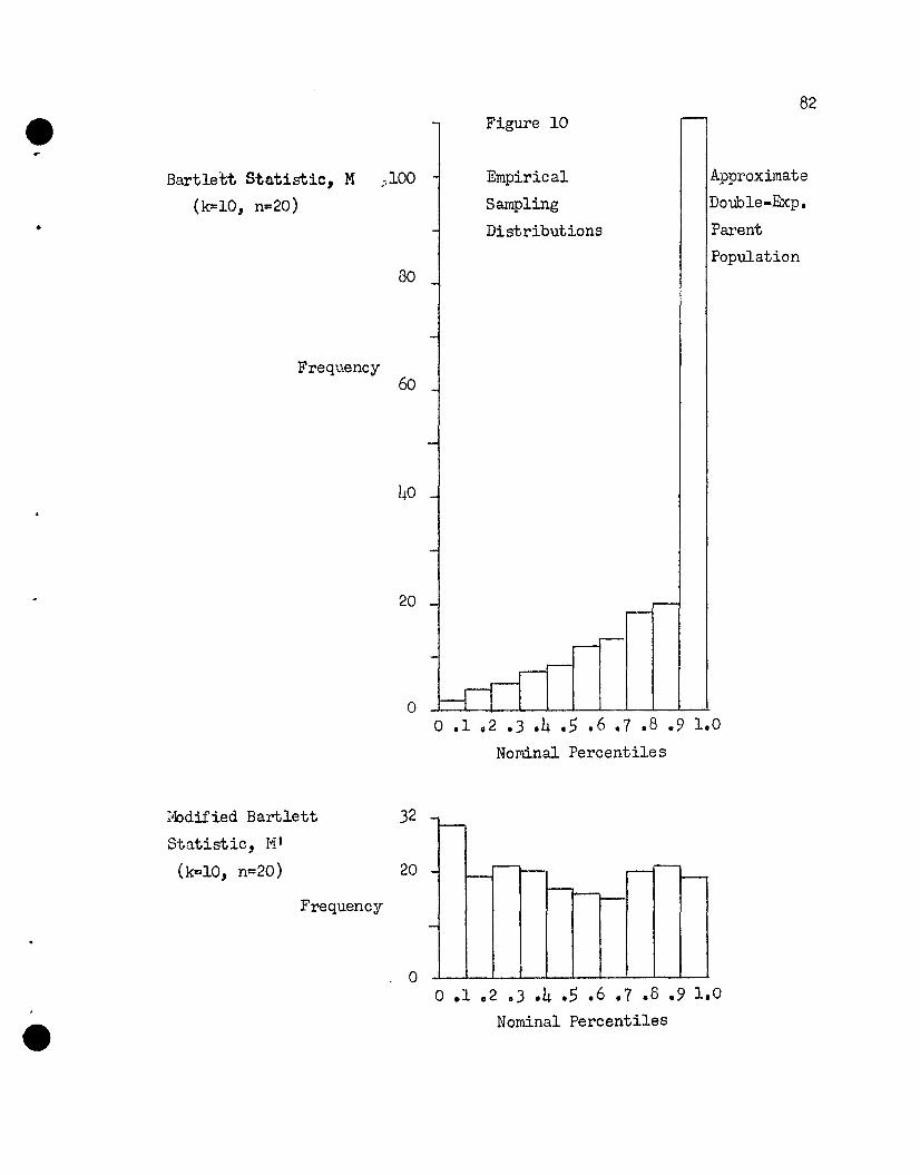
82Figure 10

•

Bartlett Statistic, M ;100

(k=lO, n=20)

80

Frequency60

40

20

o

Empirical

Sampling

Distributions

Approximate

Double-Exp.

Parent

Population

I40dified Bartlett

Statistic, 11'

(k=10, n=20)

Frequency

32

20

. 0

o .1 .2 .J .4 .5 .6 .7 .8 .9 1.0

Nominal Percentiles

o .1 02 .3 .4 .5 .6 .7 .8 .9 1.0

Nominal Percentiles

Figure 11

Empiric al Sampling Distributions

from

Normal Parent Population

83

Bartlett Statistic, M 40(kalO, n=20)

Frequency

20

o

-

-,....-. r---

I-

I- r----,--

i---- -

o .1 .2 .3 .4 .5 .6 .7 .8 .9 1.0Nominal Percentiles

•

I~dified Bartlett

Statistic, N'

(k=lO, n=20)Frequency

40

20

o

-

r-I--- -,-

r-

- -I--

- I--

--

o .1 .2 .3 .4 .5 .6 .7 .8 .9 1.0Nominal Percentiles

Bartlett StJ.tist.ic, IJI

(k=lO, n=20)

100

80

Frequency

60

40

20

o

Modified Bartlett 40Statistic, 11 1

(k=lO, n=20)

20

Frequency

o

Figure 12

Empirical Sampling Distributions

from

Rectangular Parent Population

o .1 .2 .3 .4 .5 .6 .7 .8 .9 1.0Nominal Percentiles

-_I-

r----I-- I-

- r----

o .1 .2 .3 .4 .5 ,6 .7 .3 .9 1.0

Nominal Percentiles

84

85

behavior is the occurence of 37 cases rather than the expected 20 in

the upper decile when sampling from a rectangular parent population.

However, some solace may be taken in the fact that this population

represents a more severe deviation from normallty than is commonly en­

countered in experimental situations.

Since an "idealll distribution of probabilities would give 20

samples in each decile grouping" we may make a chi square test of

the hypothesis that these empirical distributions come from a rec­

tangular distributiono The results of these computations show:

Table 13,

Empirical Comparison of The Robustness of The Two Criteria, Mand M

Parent Distribution Test Criterion Probability

..

Rectangular M 550.8 ~ooo 0001~

36.1 .000 04M

Normal M 210 2 0011 70!

e007 38M 22.9

Double Exponential M 47588 .000 0001I

6.7 0669M

While inspection of Figure 12 for the rectangular parent popu­

lation indicates that the modified statistic is much less sensitive to

0'

86

non normality than Bartlettts criterion, the significance level of

.000 04 for the chi square test indicates that we have enough evidence

here to detect the fact that Mt

is not a perfectly robust criterion.

Figure 11 for the normal population gives a significance level of

approximately .01 for both Mand Mt•

This fact plus an inspection of the individual pairs of values,of Mand M indioate that this is not so much evidence of lack of

robustness, but rather evidence of an "unlikely" set of 200 statisticso

That is, the similar failure of both graphs in Figure 11 to be rec-

tangular suggests that a repitition of this portion of the sampling

experiment would give two similar, but more nearly rectangular dis­I

tributions o Figure 10 shows that M has modified a very sensitive

test so that the new test is extremely robust to a rather leptokurtic

parent population.

While it is desirable to have a test which is more robust with

respect to non normality, it is also important that the gain in ro-

bustness is not accompanied by a great loss in power when the parent

population is normal. Therefore an equal number of samples have been

drawn from the non-null parent population (88). For the error of the

first kind fixed at ~ a .0$, the probabilities of detecting hetero-

geneity of variance of the magnitude of Hl for both the standard and

modified statistic when sampling from the normal parent population are

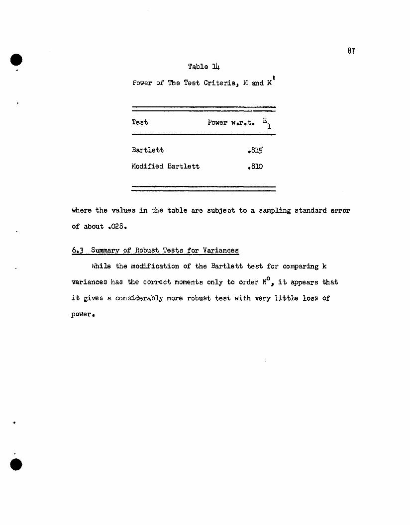
81

Table :l.4t

Power of The Test Criteria, Mand M

Bartlett .815

Modified Bartlett .810

where the values in the table are subject to a sampling standard error

of about ,,028.

6.3 Summary of Robust Tests for Variances

vmile the modification of the Bartlett test for comparing k

variances has the correct moments only to order NOJ it appears that

it gives a considerably more robust test with very little loss of

power.

Chapter VII

SUN1'~Y AND CONCLUSIONS

The primary result obtained in this dissertation is the deriva-

tion of the modified Bartlett test for comparing k variances. This

test criterion has the critical region

iVlw: NI = -";';;";1:0-

1 + ~2

2X.,< (k - 1)

where: M = N In(k2 ) - ~ nt In(k2t)

2c2 = k4 / k2

~, ~ =Fisher's k statistics

The robustness and power of this approximate permutation test

has been compared with the regular Bartlett criterion, M, by an

empirical sampling experiment. This investigation has shown that,

with no appreciable loss of power for normal parent populations, the

sensitivity of the type I error to non normality has been greatly

reduced, as the following table indicates.

Obeerved'* Type I Error, Nominal ~ = .10

Parent Population M HI

Normal .090 .130

Rectangular .005 .185

Approximate Double Exponential .555 .095'* based on 200 samples each

..

89

Having developed the idea of using approximate permutation tests

as robust testing criteria, the approximate permutation tests have been

obtained for several situations where it is desired to compare means.

The essential feature to be noted is that these criteria are the same

oas the standard tests to order N ; this explains the robustness of the

standard tests, and also serves as a justification for the standard

tests which is independent of the assumptions made in their standard

derivations. This feature is in contrast with tests to compare

variances for whi~ the normal-theory and the approximate permutation

criteria do not agree to order NO.The fact that the general (non-normal) moments may be obtained

readily from the permutation moments of these statistics enables us to

derive the effect of assumption failures in the type I error directly

from the form of the robust tests. Therefore, as a by-product of

having developed approximate permutation tests, we have a rather

simple method of evaluating the effect of non normality and variance

heterogeneity on several tests for comparing means. These results

show close agreement with previously published tables which have been

obtained by more complex methods.

In addition to these newly prepared tables, and their previously

published counterparts, excerpts have been taken from several sources

to give a more complete picture of the effects of assumption failures

on a large number of standard tests •

90

Further Research Required

The robustness of all existing par&uetric tests should be

investigated. Those showing only slight sensitivity should be desig­

nated as robust, useful procedures. Those showing great sensitivity

to the failure of the underlying assumptions should be so classified

in order that research may be initiated to find more robust procedures

for these situations. The development of new tests in this latter

situation, then, represents the second area for future research, which,

of course, must await completion of the first phaseo

In particular the large number of multivariate tests should be

studied from this point of view as there are certain to be seveIBl

tests which fall into each classification. Also the robustness of

tests in variance component analysis, regression analysis, and serial

correlation might be investigated.

In view of the failure of the modified Bartlett statistic, M',

to show as much robustness as desired, in this rather small empirical

investigation, a more extensive sampling investigation on an

electronic computer seems highly desirable. If this confirmed the

failure of HI to behave as well as might be desired, it might be

possible to develop a better statistic than MI.

91

REFERENCES

Bartlett, H.S o 1934. The problem in statistics of testing severalvariances. Proc. Camb. Phil. Soc. 30: 164-169.

Bartlett" N.S. 1936a. The information available in small samples.Proc. Camb. Phil. Soc.~: 560-566.

Bartlett, M.S. 1936b. Statistical information and properties ofsufficiency. Proc. Roy. Soc. A. f5.}~ 124-137.

Bartlett, M.S Q 1937. Properties of sufficiency and statistical tests.Froc. Roy. Soc. A. 160: 268-282.

Bartlett, M.S o 1947. The use of transformations. Biometrics 2: 39-52.

Box, G. E. Po 1951, ?h.D. thesis" University College" London. To bepublished in 1954.

Box, G. Ee Pc 1953. Non normality and toots on variances. Biometrika!±£: 318-335.

Cochran, H. G. 1947. SOIlle consequences 1rlhen the assumptions for theanalysis of variance are not satisfied. Biometrics 2: 22-38.

DaVid, F. N. 1949a. Note on the application of Fisherrs k-statisticsQBiometrika~: 383-393.

DaVid, F. i\T. 19491;>. The moments of the z and F distributions. Biometrika36: 394-403.-

DaVid, F. N. and Kendall, 1I. G. 1949. Tables of synnnetric functions.Part I. Biometrika~: 431-449.

Eisenhart , C.variance.

1947. The assumptions underlying the analysis ofBiometrics~: 1-21.

Fisher, R. A. 1935. The Design of Experiments o Oliver and Boyd,Edinburgh.

Fisher, R. A. 1936. The coefficient of racial likeness. J. Roy.Anthrop. Soc. 66: 57-63.

Gayen, A. K. 1950a. Significance of difference between the means oftwo non-normal samples. Biometrika 11: 399-407.

Gayen, A. K. 1950b. The distribution of the variance ratio in randomsamples of any size dralm from non-normal universes. Biometrika11: 236.255.

Geary, R. C.samples.

92

1936. The distribution of student 's ratio for non-normalSupp, J o R. S. s. l: 178-184.

Geary, R. c. 1947. Testing for non normality. Biometrika~: 209-242.

Kendall, H. G. 1948. The advanced Theory of Statisticsu CharlesGriffin and Company Limited, London.

Le Roux, J. 111f. 1931. A study of the q.ist ribution of variance in smallsamples. Biometrika~: 134-1900

Lehman, E. L. and Stein, C. 1949, On the theory of some non-parametrichypotre sese Ann Hath. Stat. gQ: 28-45.

Neyman, J. and Pearson, E. S. 1928. On the use and interpretation ofcertain test criteria for purposes of statistioal inference.Biometrika 20A: 175-240 and 263-294.

Neyman, J. and Pearson, E. S. 1933.tests of statistical hypotheses.

On the problem of the I1D st effie ientPhil. Trans. A. 231: 289.

Pearson, E. S.variation.

1931. The analysis of variance in cases of non-normalBiometrika~: 114-133.

Pearson, E. S. 1936. Tables of the incomplete beta-function. TheUniversity Press, Cambridge, England.

Pearson, E. S. 1937. Some aspects of the problem of randomization.Biometrika~: 53-64.

Pitman, E. J. G. 1937. Significance tests which may be applied tosamples from any population. Biometrika~: 322-335.

Rider, Pe R. 1929. On the distribution of the ratio of mean to standarddeviation in small samples from non normal populations, Biometrika21: 124-143.-

Rider, P. R. 1931. On small samples from certain non normal universes.Ann. Hath. Stat. 2: 48-65.

Sophister, 1928. Discussion of small samples from an infinite skewuniverse. Biometrika 20A: 389-423.

Tukey, J. W. 1948. Some elementary problems of importanoe to smallsample practice. Human Biology g£: 205,

Welch, B. L. 1937. On the z -test in randomized blocks and latinsquares, Biometrika. 29: 21-52.-

~jelch, B. L. 1938. On tests for homogeneity. Biometrika 22.: 149-158.

..

Appendix A

NOTES ON GENERAL TECHNIQUE OF FITTING A BETA DISTRIBUTION

BY THE FIRST TWO MOMENTS

Some relationships among the parameters and moments of the Beta

distribution should be noted. The mean and variance of a Beta variate,

with parametersI (r" s)" are known to be

I.

• rIJ. r+s

V III rs(r ... s)2 (r + s + 1)

From these it follows that

let r" s • normal-theory Beta parameters

* *r , a III parameters of Beta distribution fitted to general,

non-normal population

We have shown earlier that these may be written as

*r .. fj r

*6 III fj, S

This permits us to write

(l)

(2)

(4)

..let

* *r IJ. V~._= ...... -.

r V* IJ.

*V6 &I-

V

2(IJ.* - ~* - v*)

2(IJ. • IJ. - V)

(5)

(6)

•

94and assume

*IJ.=-IJ.

Then (,) may be written in the simpler form

26 1:1 ! (IJ. - IJ. - vs)

s 2IJ.-IJ. -v

whioh may also be wri tten in the form

6 • 1 + ~ • (1 - H)(l - e)e IJ. - 1J.2 - V

(7)

(8)

This relationship may be used to obtain the faotor, d, for robust

tests, where the Beta distribution is fitted to the permutation moments ~

* i~Then V and IJ. are the mean and varianoe with respeot to the permutation

distribution. The same relationships may be used to obtain the fa~tor,

6, for evaluating the effeot of assumption failures. The V* and IJ.*

are the mean and variance with respeot to the general (eg. non-normal)

parent population. For all the oases oonsidered in both types of pro­

*blems, it was found that IJ. 1:1 IJ. ; therefore" this assumption has been

made above to simplify the expression of 6.

(1- ~)N~

• Appendix B

CALCULATION OF THE FACTOR, d, FOR ROBUST F TESTS

This type of calculation will be illustrated by the one-way

classification of analysis of variance for comparing k means.

For reasons noted earlier, we shall consider the statistic,

W a:s treatment awn of squarestreatment + error awn of squares

From Welch (1938) we have the moments of W.

Permutation Moments:

v* • l~ 1:1 2(k - l)(N - k)(N + l)(N _ 1)2

.~ (l.(N _ 1)2~ N

Normal-Theory Moments.

~ 1:1 ~(N) 1:1 k - 1N - 1

v 1:1 ~ (N) 1:1 2(k - l)(N - k)2 (N +. l)(N _ 1)2

(1)

(2)

(3)

(4)

(5)

where I n 1:1 nwnber of observations per groupt

k~N A ~ nt 1:1 total nwnber of observationstal

96

With the moments given in (3) and (5), we write equation A(6) for this

case

v*e III -.

V°2(1 .. -)N

k2 ~ 1o(--~- )2 N n

t

2(k .. l)(N .. k)N + 1

(6)

where:

•

By the use of equation A(8) we may then write

N + 1 N + 1NeN .. 11 +. ~ U

d III 1 + 021

1 .. c2 ( N.. U)

where:

1 k2 1U :I N_+ ( _ .. ~ _ )

2(k .. l)(N .. k) N nt

For large N, this may be approximated by

d-l+ l+NUN .. 02 + NU02

For equal sized groups, where U III 0, we have

(N + 1)02d III 1 + -------

(N .. l)(N - 02)

(7)

(8)

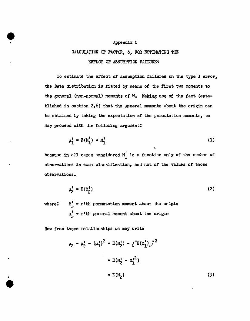
, Appendix C

CALCULATION OF FACTOR, 6, FOR ESTIMATING THE

EFFECT OF ASSUMPl'ION FAILURES

To estimate the effect of assU1T1ption failures on the type I error,

the Beta distribution is fitted. by means of the first two moments to

the general (non-normal) moments of W. Making use of the fact (esta­

blished in section 2,6) that the general moments about the origin can

be obtained by taking the expectation of the permutation moments, we

may proceed with the following argument:

(1)

because in all cases considered M~ is a function only of the nU1T1ber of

observations in each classifieation, and not of the values of those

observations.

Where: M' • r1th pemutation moment about the originr

~' • r'th general moment about the originr

(2)

•

Now trom these relationships we may write

• E(~) (3)

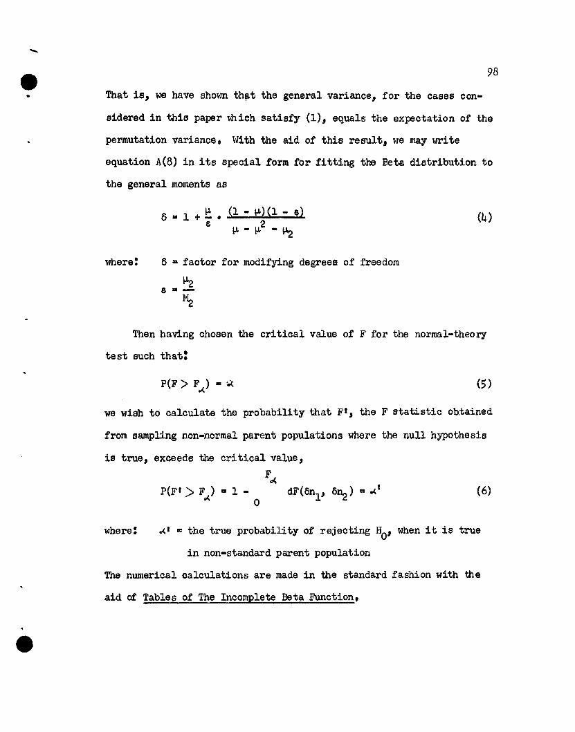
..98

That is, we have shown th~t the general variance, for the cases con-

sidered in this paper mich satisfy (1), equals the expectation of the

permutation variance. With the aid of this result, we may write

equation A(8) in its special form for fitting the Beta distribution to

the general moments as

where:

8 • 1 + ~ • (1 - ~)(l - e~e ~ _ ~2 _ ~

6 D factor for modifying degrees of freedom

(4)

Then having chosen the critical value of F for the normal-theory

test such that:

(5)

we wish to calculate the probability that Ft, the F statistic ob.tained

from sampling non-normal parent populations where the null hypothesis

is true, exceeds the critical value,

F.,((6)

where: .,(,1 III the true probability of rejecting HO

' when it is true

in non-standard parent population

The numerical oalculations are made in the standard fashion with the

aid of Tables of The Incomplete Beta Function,

•

99

Having established the general method, consider a particular

case, the one-way classification analysis of variance, with an equal

number of observations in each group. From equation (J), we may write

v* 1:1 ~(G) 1:1 E(M_) D 2(k-l) (N-k) [1 - 1 E(c ) 7 (7). ~ -~ (N+l) (N_1)2 N 2-

Therefore the only change in the modifying factor, d, for the robust

test, and the factor, 0, for evaluating non-normality is replacement

of 02 by E(02)o Therefore

(N + 1) E(02)o a 1 + ---------

(N - l)(N - E(02) )(8)

To find E(02) in terms of the population parameters, write "2 in the

form,

Letting /), • k - Kr r r

and using the series expansion

1 =1 _ 2z + 3z,2 _ 4z3(1 + z)2

we may rewrite (9) in the form

+ 0 ••

0 •• 7- (10)

100

Using the method of evaluating moments and mixed moments of k-statis­

tics by F. N. David (1949), the expectation of c2 to order 1'1-1 is

where:

K +2A .....r--.;.__r r+2

~T

K • r1th cumulantr

Substituting (11) into (8) and simplifying" we have

(1'1 + 1) E(c2

)8 • 1 + -----=-----

(1'1 • 1) L-N - E(c2).7

2E(c2) + N(N - 1)---.;;.------(N - 1) L-N - E(02).7

(ll)

(12)

(13)

Since E(c2) has been evaluated only to order N-l and since If is

large relative to E(c2 )" this may" for practical purposes~ be approxi­

mated by the simpler expression,

...

8 • _.....;;;1-:--_E(c2 )

1 - _..::-N

(14)

Appendix D

METHOD OF CONSTRUCTION OF CRITICAL REGION FOR THE

APPROXD1ATE PERMUTATION TEST" SECTION 2.10

The procedure for obtaining the cross section of the critical

region" W, on the plane"

of the approximate permutation test is outlined. Since the critical

region, W" is defined by

those points on the boundary of W.,t. will be defined by

Since

(1)

(2 )

and

(n + 2 )(b2 - 3)d • ----..;;;--

n(n + 2 - b2 )

5(b2 - 3)• --=----3(5 - b2 )

(J)

it is possible to draw contour lines of constant d.

Also, F is defined as a function of the sample by

(4)

(5)

102

Figure 13

7

9

4

10

5

3

1

o

2

...-

· -.. 6• • <

• loa ....

o .'.-......o '.· '.· '.o •· ..· .'· .'·.'

..+..... : •• "

• <C"..... ...... : ..... . ....;.... : ...:..... .... .. ." If·.e •••• : ...... : .......-....... : .,.. loa. .... II .......

: .... : ........:'.... : ...

Graphical Construction

of

Approximate Permutation Test

Critical Region

10

Concentric Circles =Contours of Equal F.10 (b2)

Other Contours of Equal b2, i.e. equal d.

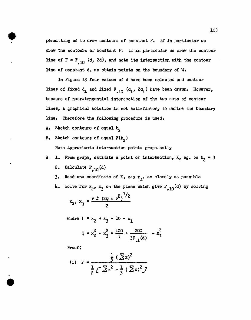
103

permitting us to draw contours of constant F. If in particular we

draw the contours of constant F0 If' in particular we draw the contour

line of' F • F.10 (d, 2d), and note its intersection with the contour

line of constant d, we obtain points on the boundary of W.

In Figure 13 four values of d have been seleoted and oontour

lines of fixed di and fixed F.10 (di , 2di

) have been drawn. However,

beoause of near-tangential interseotion of the two sets of oontour

lines, a graphioal solution is not satisfaotory to define the boundary

line. Therefore the following procedure is used.

A. Sketch contours of equal b2

B. Sketch contours of equal F(b2 )

Note approximate intersection points graphically

Bo 1. From graph, estimate a point of intersection, X, ego on b2 a 3

2. Caloulate F.10(d)

3. Read one coordinate of X, say Xl' as closely as possible

4. Solve for ~, x3

on the plane which give F.10(d) by solving

p :t (29 _ 1-)1/2x2' x3 ... 2

where P a X2

+ X3 III 10 .. Xl

2 2 • !QQ. + 200 2Q ... X2 + X3 3 3F.l (d)

.. Xl

Proof:

(i) F •j (~X)2

! ( ~ X2 _ ! (~x)2 7

23-.-

e

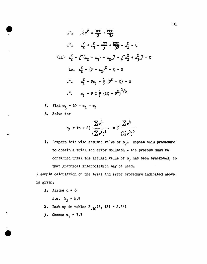
•• • Y. x2 • 100 + gQQL.J 3 3F

• ~ + x2D !QQ. + 200 _ x2

1:1 ()

•• -~ 3 3 3F 1 ~

(ii) ~ + L-(~ + x3) - x2...7 - L-x~ + x~_7 .. 0

104

1e.

•• •

•• •

2 1 2~ - ~ + 2' (I' ... Q) 1:1 0

1 _2 1/2~ • P i 2' (2Q ... 1')

•

5. Find x3 • 10 - xl ... ~

6. Solve for

~x4(n + 2) --­

(~x2)2-5---

(~x2)2

1. Compare this with assumed value of b20 Repeat this procedure

to obtain a trial and error solution ... the process must be

continued until the asswned value of b2 has been bracketed, so

that graphical interpolation may be used.

A sample calculation of the trial and error procedure indicated above

is given.

1. Assume d 1:1 6

i.e. b2 =405

2. wok up in tables F.lO (6, 12) • 2.331

3. Choose Xl • 1.1

4. Calculate

P • 10 - 1.1 1:1 2.3

105

•

•

• 10 15

5. Solve for

X3 1:1 10 - 1.7 - 1.15 • 1.15

6. From these we calculate the sample value"

b2 1:1 4.587

7. Compare this to the assumed value b2 = 40500 and choose a

new estimate xl to decrease the calculated value 4.587

nearer the assumed value" 40500 •

The results of these calculations for four contours of equal d

values are:

b2 d xl ~ .2- F.10(b2)- -2.143 0.50 3000 4055 2.45 28.123

3.000 11100 5.56 2.67 1.17 8.526

4.500 6.00 1,61 0.66 7.67 2.331

4.945 60.00 0.23 0.64 9.13 1 0 3203

Appendix E

DERIVATION OF ROBUST F TEST FOR COMPARING

TWO VARIANCES, MEANS KNOWN

Consider the statistic,

nl 02

ni

·~2 ~~2W .. &J Xl' .&:i ~ X .

j=l J illll j=l iJ(1)

with the assumption that

2IN (0, (j.)J.

and under the null hypothesi s

(2 )E(U) • I-L(N)

it is well known then that Whas a Beta distribution vdth parameters,

(ny'2, ~/2)" enabling us to write the moments,

nlD_

N

where:

(4)

•

Noting that the denominator of Wis constant over all permutations of

the observations, we find the permutation moments,n

l-51\ D N 2

82

where:

2 ni

S ... ~ .~ X:jr i=l j=l J.

107

The second permutation moment with respect to the origin is

Noting that

4 1E(X ) • N84

E(Xi X~) = E(Xi) • E(~ / xi)E(Xi) • (52 - xi>.-~-------

N - 12

52 - S4=-_......N(N - 1)

Now using (6) and (7) to evaluate (5), we have

(5)

(6)

(7)

where:

(8)

From this it follows that

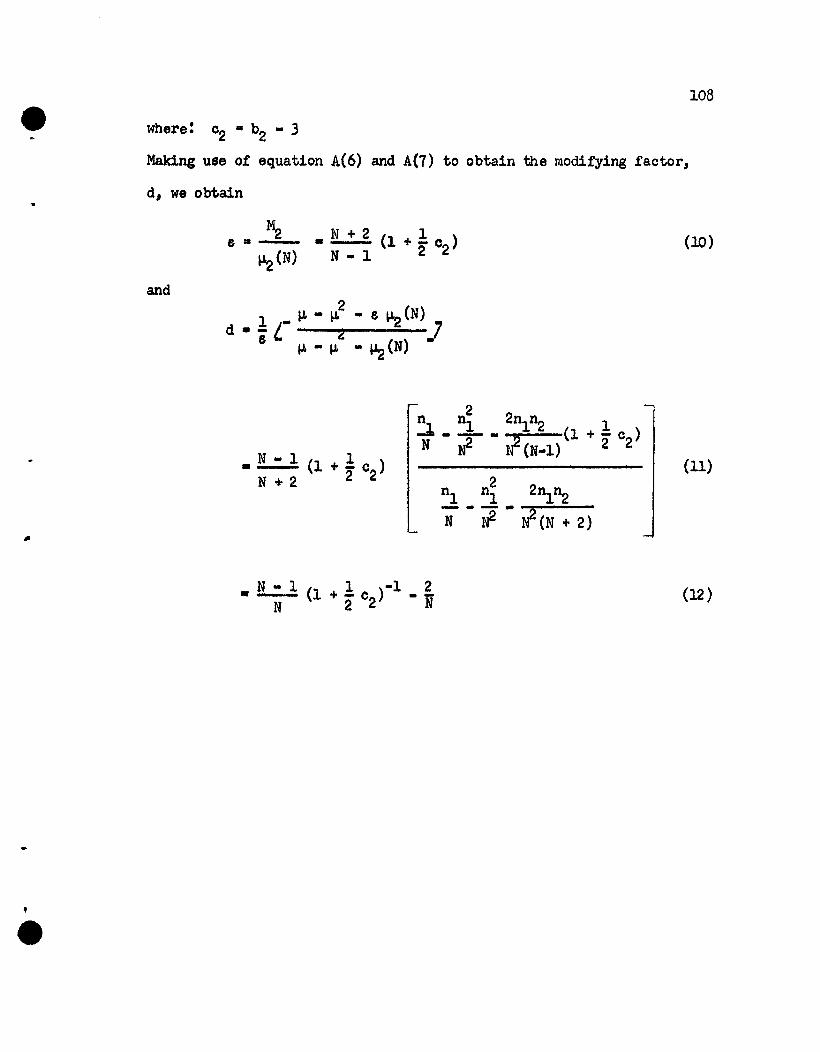
108

where: O2 III b2 - 3

Making use of equation A(6) and A(7) to obtain the modifying factor,

d, we obtain

~e ..~(N)

and

• N + 2 (1 + ! c )N _ 1 2 2

(10)

21 ~ - ~ - e ~(N)

d • - L- 2 7e ~ _ ~ _ ~(N) -

• N - 1 (1 + ! 0 )N + 2 2 2

• N - 1 (1 + ! 0 )-1 _ £N 2 2 N

(11)

(12)

Appendix F

DERIVATION OF IJiODIFIED BARTIETT STATISTIC, M',

MEANS UNKNCMN

For the case where the means of the k groups are assumed known,

there will be no loss of generality to consider these means all zero.

Adopt the notation

kM .. n In(m) - ~ nt In(m

t)

t-lk m

.. - .~ nt

In(..1)t-l m

(1)

where:

m

N

1 ~ 1= - .2 n m =-S

N tel t t N 2

= number of observations per sample

= number of groups

c: ~ nt

=total nwnber of observationst=l

= i-th observation in t-th group

k nt N.~ ]y~ =~y2

tal i=l 1t a=l a

letm - m

xt

:= _t--m--

Then we may rewrite (1) in the form

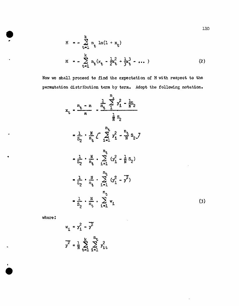
k

M .. - ~ n 1n(1 + Xt )tal t

k

M =.. ~ n (x - k 2+ 1:x3 - ••• )

t=l t t 2 t 3 t

110

(2 )

Now we shall proceed to find the expectation of Mwith respect to the

permutation distribution term by term. Adopt the following notation.

nt1 N

~2 1

a- .- . (Yi .. N52)52 nt i=l

nt2 2'.1.. • .!-. :2

52 nt i=l(Yi - Y )

nt1 N ~w-- .- .52 nt iq:a1 i

where:

k nt;Z =1: ~ ~ y.~

N tal 1=1 lot

III

Now let us evaluate the first term in the series expansion of M.

This by inspection is zero. Then writing the second term we have

Using equation (J), we write

(4)

•Now consider some sub calculations which must be made before proceeding•

Type A Calculation - Expectations of powers and products of WiS.

All expectation operators will be with respect

to the permutation distribution.

where:

2 1E(w ) • - s 'N 2

E(WiWj ) ~ E(wi ) • E(wj / wi) • E(wi ) •

-E(w~)• 1 ~ _ 1 5 I

N - 1 N(N • 1) 2

S I - w1 i

N - 1

(5)

(6)

(7 )

..

noting that

Type B Calculation - Express Sk I in terms of sums such as Sr' and

standardized moments, br -

N NS'

~ 2 ~ 21222 &I ~ W • ~ (y _ ... 52)a&ll a a=l a N

~ _2 2 2 1 2... ~ Ly - - S2 Y +:2 82_7a=l a NaN

1 2I:J 54 - - 5N 2

Dividing through by s~, equation (9) may be written in the form

where:

Returning to the main argument of evaluating the expectation of the

second term in the serie s expansion, we have

112

(10)

11)

E(ll) .! 2n • i . .;. .[~s I _ nt (nt - 1) 5 1 ]

2 tllll t n~ S~ N 2 N(N - 1) 2t 2

Type C Calculation - Series expansion of ooefficients

To simplify expressions of the type above, it will be helpful to

adopt a uniform way of combining coefficients, for which the following

notation will be of assistance.n

Ist A. ::io N

nt(nt - 1)A • ---............--1 N(N - 1)

nt(nt - 1) ••• (nt .- r)A ... -:..--=-----~--r N(N - 1) ••• (N • r)

Returning to the main argument, we have

.! ~ i (,4.- • A ) • -N1(b2 - 1)2 t-l nt -U 1

-1Taking terms of A1 to order N ,we get

(11)

1 N=2(b2 ... l)(k ... l} " ----­N ... 1

q" e" do E(ll)

Following this prooedure gives to order N-l

114

(12)

: _-..tl__ . (k-l) 0 (

3 (N-1) (N...2)

and

(13)

C . ...1o11ectJ.ng tams gives to order N

(15)

115

To find the variance of M, first evaluate the expectation of

M2, which as a conse~ence of (2), may be written directly as

~n~~

(III)

+~~~ 2 2 l'~ ~ 2 3nnxx -- ~ ntnsxtxst ,t s t s t s 3 t:fS

(IV) (V)

+1 ~ ~ n n x2x4 +1 ~ ~ ntnsx~x; + • tt •4 t s t s 9 . .'J

t r s t :f s(VI) (VII)

(16)

Following the pattern of finding the mean of M, we shall evaluate the

first term in some detail and give the results for the rest. The

first tem may be written

•

k1 ~ 2 4

I = -4 ~ nt xtt=l

With the aid of (3) we write

TlPe D Calc~_ation

(11)

(18)

By the usa of tables of symmetric functions by F. NO) David and

1>1. G. Kendall (1949) expressions of the follcwing type may be evaluated

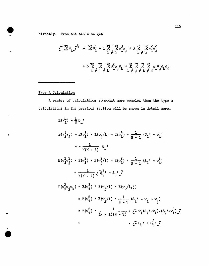
116

directly. From the table we get

•

~4 ~.~':l v·~22= ~wi + 4..:::J ~ w;.w. + 3~ ~ w. w.ifj J ifj J.J

•

Type A Calculation

A series of calculations somewhat more complex than the type A

calculations in the previous section will be shown in detail here.

E("r?w.) III E(w3.i ) • E(wj/i) ... E(~?) • --L. (Sl' - wi)J.J J. N-l

... _ 1 S 'N(N - 1) 4

22 2 2 2 1 2E(wiwj ) ... E(wi ) • E(wj/i) ... E(wi ) • N _ 1 (52' - wi)

... 1 1.-62 , N S ' 7N(N - 1) 2 4 -

2 2E(WiWjwk ) =E(wi ) • E(wj/i) • E(w~i,j)

... E(W~) • E(w Ii). 1 (5 1 - w - w )J. j N-2 1 i j

... E(w2 ) • 1 ./..: w.(S l-w.)-(8 I_W2) 7i (N _ 1)(N _ 2) J. 1 J. 2 i-

= • I.: s 1 + 52 1 72 2 -

111

1=-------N(N - l)(N - 2)

= P •

•

E(WiWjWkWe) ... E(wi ) , E(wj/i) • E(wk/i,j) • E(We/i,j,k)

(P) (Q) (R) (T)

&:: P Q R' 1 L-s' - wi - wJ. - W 7N _ 3 - 1 k-

IS P Q • _..-...;:1:-.-_ L=wi (Sl '-W. -w. )-w. (51' -wi-w. )(N-2 )(N-3) J. J J J

2 2 J- (S2'-wi -wj )

a P Q • 1 L-2.w~ + 2w~ + 2w.w. - S2' 7(N-2 )(N-3) J. J J. J -

1 L-2W~ (51' -w.) + 2 (53 ' -w? )(N-l)(N-2 )(N-3) J. J. J.

+ 2w. (s ,_w2 )_S '(8 '-W ) 7J. 2 i 2 1 i-

... p • __--:;.1 r -6w~ + 3w.S , + 2S , 7(N-l)(N-2 )(N-3) " J. J. 2 3 -

.. 1 ,-382 , _ 6S , 7N(N-l)(N-2) (N-3) 2 4 -

Type C Calculation

Because of the greater complexity of the evaluation of the

variance, and because we are seeking an answer correct only to order

N-l J we shall expand slightly on the type C calculation illustrated in

the previous section. There we adopted the notation of (11).

118

nt(nt - 1) ••• (nt - r)A II ...;..-..;.------=;....---r N(N - 1) ••• (N - r)

In evaluating the variance we shall rewrite these coefficients as

Returning to the main argument as we left it in (18), and making

use of the auxiliary calculations, D, A, and 0, we may write

•We now wish to express the Sr' in terms of the ~; therefore we perform

another

119

TyPe B Calculation

S4 I = ~ w4 = ~ (l - k 2 )4a=l a a=l a W-

= ~a=l

where:

•

In a similar manner or by using (10), we have

S2.2 1 2- =~ (b - 1)s4 NC:: 22

Again returning to the main argument as we left it in (19), we have

kE(I) =~ .~ ~ [N(b6 - 4b4 + 6b2 - 3)(Ao - 7Al + 12A2 -6A3 )

t-l nt+ ~(b2 - 1)2 (3Al - 6~ + 3A3) ]

= t(b2 - 1)2 (3k - 6 + 7~ n~)

1 [ "'1 6 ~ 2+ - (b6 - 4b4 + 6b2 - 3)(N ~ - - 7k + 12 - 2'~ nt )4N nt N

2~1 18 ~ 21+ (b2 - 1) (-3N..Gii\' + 2lk - 36 + 7~nt)_

q. e. d. E(l)

120

(20)

•

In a similar manner we may calcula te the remainder of the terms

in (2). The results of these calcuJa tiona are

1 2 - ~n~ 7E(IV) • [(b2 - 1) Lk(k - 1) - 2(k - 1) + 3(1 - ~ )_

+,L k(k-l) (k-1) 1 ~ 2(1 -l~nt)4N

- 1 + 4 - 6 b6

+4 -16 +24 b4

+ 3 -12 +16 b22

-12 +46 -12

~+ 6 -24 +36 (1)

E(V) = - ~ L-b4b2 - 3b~ + 5b2 - b4 - 2.7 •L-N(k-l) ~~

- (N~~ - k)- 6k(k-l) + 20(k-l)- 20(1 -7~ n~)_7

E(lll) =~ L-b~ - 3b~ + 3b2 - 1_7·L-15N2~ -45k+4'-J]ni_7

..E(VI) • -91N ;-"b2

3 - 3b22

+ 3b2 - 1 7./"3Nk ~!.. - 6N~1-• • - nt nt

2 1 ~ 2 7+ 30k - 6k - 36 + 157~nt_

E(VII) • tN l.-b2 - 1_73 • L-_9k2

+ 27K - 33 + 157~ n~_7

-2Further terms in the series expansion 8ive terms only to order N •

Noting the relationship

we proceed to collect te~ and obtain

b - 1V(M) • 2(k - 1)( 2 2 )2 + terms ot order H-l

which may be tabulated as tollows.

Terms ot order H-l in V(M) •

121

1-.36N

N~!..ntb6 + 9

b4 + 72

b4b2 -108

b3 +1682b2 -2072

b2 + 72

(1) - 6

- 9

+36

-36

+ 9

'k (1)

-.18 + 18

-ll,4 + 72

+216 -144-288 +lS6

+306 -108

- 72

+ 6

•

Appendix G

DERIVATION OF MEAN AND VARIANCE OF MODIFIED

BARTLETT STATISTIC, MEANS UNKNOWN

Bartlett's statistic may be written in the form

(1)

where: ~t ... Fisher's k statistics, sample variance for t-th group

~ III Weighted average sample variance for k groups

Write the sample variances in the form

where:

~ = K2

(1 + ~ - ~) 1;1 K2

(1 + t)K

22

2~ ... population 2-nd cumulant, a

~"'~-K2

(2 )

Recall the series expansion

In (1 + x) ... x - ! x2+ ! x3 -

2 3

which permits us to write

• • •

Now consider the modifying factor

•

123

Since /c2/ < 1 with high probability, we may write the series expansion

Since c2 itself is a ratio of two random variables, it is necessary to

obtain a series expansion of its denominator as follows:

where: k4 =Fisher's fourth k statistic

K4 • fourth population cumulant

(6)

Without loss of generality we may assume K2 =1 and then write

where: 6r

=k -Kr r (r = 2,4)

Combining the three aeries expansions, (4), (5) and (7), we may write

the modified Bartlett statistic, M', as

M' = --..;.MT1- • L-~( ~nt~t • N~) - j(~nt~t - N~)1 + 2'c2

+ ~( ) .. e.7XL-l - ~(K4+64)(1 - 2~ + 3~ -... )

r

e1 2 2 2 1

+ 4(K4 + 64) (1 - 2~ + 362 - ... ) -"8." (8)

+ •• ,.7

•

-1 ~ 2 2 1 ~ 3 2= /. 2(~nt~t· NA2) - 3(~ntA2t - NA2)

x L-1 . ~4 + (~4)2 - (~4)3 + •••

• ~ \ + K4~ + ~4~ • •...7

124

•

By use of the teohnique of F. N. David (1949) to evaluate the expecta-

tiona of powers and cross products of the ~ funotions J the expected

value of MI to order NO may be found. From these tables it is

immediately apparent thij.t for powers and cross products of the ~IS of

order three and greaterJ the expectations are of order N-l or greaterJ

so that we need consider only terms of order two in the ~ts. There-

fore we may shorten (9) to

- •.. 7.. (10)

(11)

Now taking expectations with the aid of David I s tables.. we obtain

(12 )

• k • 1 Q.ee cd. expectation

,

-

By use of the same three series expansions we find the variance of

Mt to order NO to be

(13)

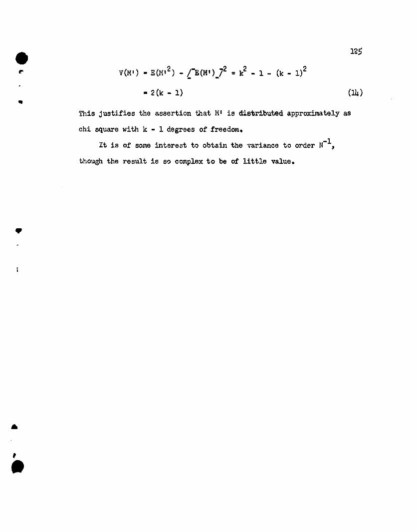
125

2 -,." 72 2 2V(M') =E(MI ) - / ~(Mt) = k - 1 - (k - 1)- -• 2(k - 1) (14)

•

,•

This justifies the assertion that MI is distributed approximately as

chi square with k - 1 degrees of freedom.

It is of some interest to obtain the variance to order N-l ,

though the result is st) complex to be of little value •