robust underwater obstacle detection and avoidance...
TRANSCRIPT
ROBUST UNDERWATER OBSTACLE
DETECTION AND AVOIDANCE
VARADARAJAN GANESAN
(B.Eng.(Hons))
A THESIS SUBMITTED FOR THE DEGREE OF
MASTERS OF ENGINEERING
ELECTRICAL AND COMPUTER ENGINEERING
NATIONAL UNIVERSITY OF SINGAPORE
2014

DECLARATION
I hereby declare that this thesis is my original work and it has been written by
me in its entirety.
I have duly acknowledged all the sources of information which have been used
in the thesis.
This thesis has also not been submitted for any degree in any university
previously.
Signed:
Date: 03-11-2014
i

“Everything should be made as simple as possible, but not simpler”
Albert Einstein
Acknowledgements
The research described in this thesis was not a solitary effort. A lot of
people have contributed directly and indirectly to it for which the author is very
grateful to each one of them.
I wish to express my sincere thanks and appreciation to my supervisor,
Prof. Mandar Chitre for his invaluable guidance, support and timely suggestions
without which this thesis could not have been completed.
I am also indebted to the members of the STARFISH team for being very
helpful throughout the course of my research. In particular, I would like to thank
Yew Teck Tan, Bharath Kalyan, Koay Teong Beng and Edmund Brekke for their
support and valuable suggestions on my work. I also thank the larger Acoustic
Reserach Lab (ARL) community for supporting the research carried out in this
thesis and for creating a great environment to work in.
Finally, I would like to thank my family and friends for their constant love,
support and encouragement throughout the past two years.
iii
Contents
DECLARATION i
Acknowledgements iii
Table of Contents iv
Summary vi
List of Tables viii
List of Figures ix
List of Abbreviations xi
List of Symbols xii
1 Introduction 11.1 Motivation . . . . . . . . . . . . . . . . . . . . . . . . . . . . . 11.2 The STARFISH Project . . . . . . . . . . . . . . . . . . . . . . 41.3 Approach . . . . . . . . . . . . . . . . . . . . . . . . . . . . . 71.4 Thesis Layout . . . . . . . . . . . . . . . . . . . . . . . . . . . 8
2 Background 92.1 Image Processing Techniques . . . . . . . . . . . . . . . . . . . 102.2 SLAM Techniques . . . . . . . . . . . . . . . . . . . . . . . . 132.3 Occupancy Grids . . . . . . . . . . . . . . . . . . . . . . . . . 152.4 Summary . . . . . . . . . . . . . . . . . . . . . . . . . . . . . 17
3 Underwater Obstacle Detection 193.1 Preliminary . . . . . . . . . . . . . . . . . . . . . . . . . . . . 193.2 Occupancy grid . . . . . . . . . . . . . . . . . . . . . . . . . . 223.3 Measurement Model . . . . . . . . . . . . . . . . . . . . . . . 233.4 Motion model . . . . . . . . . . . . . . . . . . . . . . . . . . . 26
3.4.1 Translational Motion . . . . . . . . . . . . . . . . . . . 27
iv
Table of Contents
3.4.2 Rotational Motion: . . . . . . . . . . . . . . . . . . . . 303.5 Detection Procedure . . . . . . . . . . . . . . . . . . . . . . . . 313.6 Summary . . . . . . . . . . . . . . . . . . . . . . . . . . . . . 31
4 Results on Obstacle Detection 334.1 Experimental Setup . . . . . . . . . . . . . . . . . . . . . . . . 334.2 Noise Distribution . . . . . . . . . . . . . . . . . . . . . . . . . 364.3 ROC curves, operating pk and tk . . . . . . . . . . . . . . . . . 394.4 Scan Results . . . . . . . . . . . . . . . . . . . . . . . . . . . . 404.5 Summary . . . . . . . . . . . . . . . . . . . . . . . . . . . . . 46
5 Command and Control Architechture for STARFISH AUV 475.1 The C2 Architecture . . . . . . . . . . . . . . . . . . . . . . . 475.2 Obstacle Avoidance . . . . . . . . . . . . . . . . . . . . . . . . 52
5.2.1 FLSDetector . . . . . . . . . . . . . . . . . . . . . . . 525.2.2 Navigator . . . . . . . . . . . . . . . . . . . . . . . . . 52
5.3 Summary . . . . . . . . . . . . . . . . . . . . . . . . . . . . . 58
6 Results on Obstacle Avoidance 596.1 Simulation Studies . . . . . . . . . . . . . . . . . . . . . . . . 59
6.1.1 Results . . . . . . . . . . . . . . . . . . . . . . . . . . 606.2 Experimental Results . . . . . . . . . . . . . . . . . . . . . . . 656.3 Summary . . . . . . . . . . . . . . . . . . . . . . . . . . . . . 69
7 Conclusions and Future Work 727.1 Conclusion . . . . . . . . . . . . . . . . . . . . . . . . . . . . 727.2 Future Work . . . . . . . . . . . . . . . . . . . . . . . . . . . . 73
7.2.1 Dynamic Targets . . . . . . . . . . . . . . . . . . . . . 737.2.2 Sea Trials . . . . . . . . . . . . . . . . . . . . . . . . . 747.2.3 Intelligent C2 System . . . . . . . . . . . . . . . . . . . 747.2.4 Global Avoidance . . . . . . . . . . . . . . . . . . . . . 74
7.3 A Final Word . . . . . . . . . . . . . . . . . . . . . . . . . . . 75
Bibliography 76
Publications 80
v
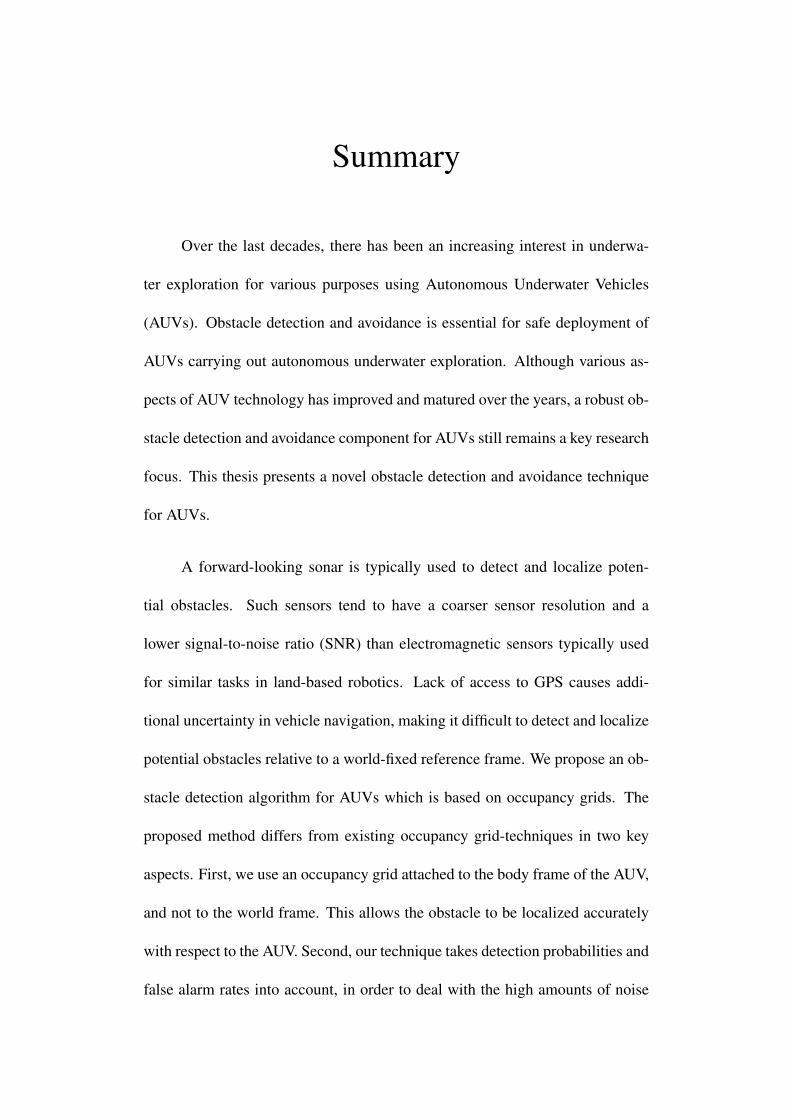
Summary
Over the last decades, there has been an increasing interest in underwa-
ter exploration for various purposes using Autonomous Underwater Vehicles
(AUVs). Obstacle detection and avoidance is essential for safe deployment of
AUVs carrying out autonomous underwater exploration. Although various as-
pects of AUV technology has improved and matured over the years, a robust ob-
stacle detection and avoidance component for AUVs still remains a key research
focus. This thesis presents a novel obstacle detection and avoidance technique
for AUVs.
A forward-looking sonar is typically used to detect and localize poten-
tial obstacles. Such sensors tend to have a coarser sensor resolution and a
lower signal-to-noise ratio (SNR) than electromagnetic sensors typically used
for similar tasks in land-based robotics. Lack of access to GPS causes addi-
tional uncertainty in vehicle navigation, making it difficult to detect and localize
potential obstacles relative to a world-fixed reference frame. We propose an ob-
stacle detection algorithm for AUVs which is based on occupancy grids. The
proposed method differs from existing occupancy grid-techniques in two key
aspects. First, we use an occupancy grid attached to the body frame of the AUV,
and not to the world frame. This allows the obstacle to be localized accurately
with respect to the AUV. Second, our technique takes detection probabilities and
false alarm rates into account, in order to deal with the high amounts of noise
Summary
present in the sonar data. This local probabilistic occupancy grid is used to ex-
tract potential obstacles which is then sent to the command and control (C2)
system of the AUV. The C2 system checks for possible collision and executes
an evasive maneuver accordingly.
The proposed algorithm was tested during field trials at Pandan Reservoir
in Singapore and at Selat Pauh, an anchorage off the coast of Singapore. We used
an AUV built by the Acoustic Research Laboratory (ARL) under the National
University of Singapore, mounted with a Micron DST sector scanning sonar
during the experiments.
vii

List of Tables
3.1 Detection Table . . . . . . . . . . . . . . . . . . . . . . . . . . 21
viii
List of Figures
1.1 Redstar and Bluestar during field trials . . . . . . . . . . . . . . 51.2 Micron DST sector scanning sonar . . . . . . . . . . . . . . . . 61.3 Illustration of the working of a sector scanning sonar . . . . . . 6
2.1 Raw scan of a coral reef using a sector scanning sonar . . . . . . 132.2 Illustration of a global occupancy grid . . . . . . . . . . . . . . 162.3 Illustration of a local occupancy grid . . . . . . . . . . . . . . . 16
3.1 Flow chart showing the flow of control during the obstacle de-tection stage . . . . . . . . . . . . . . . . . . . . . . . . . . . . 20
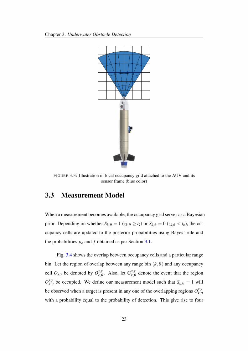
3.2 Echo intensity, zk,θ vs Range bins, k for a given FLS scan bearing 213.3 Illustration of local occupancy grid attached to the AUV and its
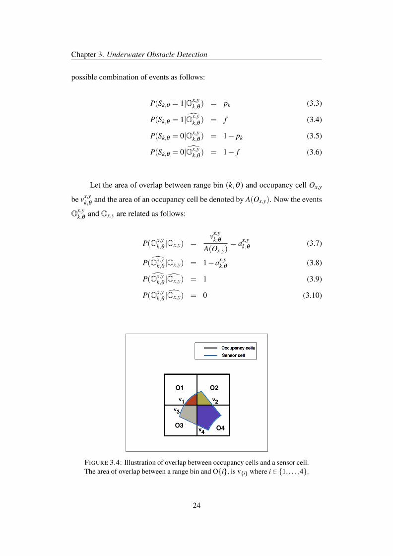
sensor frame (blue color) . . . . . . . . . . . . . . . . . . . . . 233.4 Illustration of overlap between occupancy cells and a sensor
cell. The area of overlap between a range bin and O{i}, is v{i}where i ∈ {1, . . . ,4}. . . . . . . . . . . . . . . . . . . . . . . . 24
3.5 Illustration of overlap of neighboring occupancy cells after un-dergoing translation with a particular occupancy cell. The areaof overlap between O-new and O-{i}, is w-{i}where i∈{4,5,7 and 8}. 28
3.6 Graphical Representation of Kernels . . . . . . . . . . . . . . . 293.7 Illustration of overlap of neighboring occupancy cells after un-
dergoing rotation with a particular occupancy cell. The area ofoverlap between O-new and O-{i}, is w-{i}where i∈{2,4,5,6 and 8}. 30
4.1 STARFISH AUV . . . . . . . . . . . . . . . . . . . . . . . . . 344.2 Illustration showing the structure of embankments at Pandan
reservoir . . . . . . . . . . . . . . . . . . . . . . . . . . . . . . 344.3 Experiments at Pandan reservoir and at sea . . . . . . . . . . . . 354.4 Distribution of Background Noise at Pandan Reservoir . . . . . 374.5 Distribution of Background Noise at Selat Pauh . . . . . . . . . 384.6 Experimentally obtained ROC plots. . . . . . . . . . . . . . . . 414.7 Experimentally obtained operational pk vs range bins, k. . . . . 424.8 Experimentally obtained operational tk vs range bins, k. . . . . . 43
ix
List of Figures
4.9 Unprocessed scans (left column), occupancy grid (middle col-umn) and obstacle detection (right column) of the reservior’sembankments during the Pandan experiment. . . . . . . . . . . 44
4.10 Unprocessed scans (left column), occupancy grid (middle col-umn) and obstacle detection (right column) of the coral reef dur-ing the sea experiment. . . . . . . . . . . . . . . . . . . . . . . 44
4.11 Unprocessed scans (left column), occupancy grid (middle col-umn) and obstacle detection (right column) of a buoy during theexperiment at Pandan reservoir. . . . . . . . . . . . . . . . . . . 45
5.1 Overview of Command and Control System [26] . . . . . . . . 485.2 Mission points and waypoints for a mission planned at Pandan
reservoir . . . . . . . . . . . . . . . . . . . . . . . . . . . . . . 515.3 Flow chart showing the flow of control during the obstacle avoid-
ance stage . . . . . . . . . . . . . . . . . . . . . . . . . . . . . 535.4 Detection maps . . . . . . . . . . . . . . . . . . . . . . . . . . 545.5 Waypoints . . . . . . . . . . . . . . . . . . . . . . . . . . . . . 555.6 Collision Checking by Navigator . . . . . . . . . . . . . . . . . 57
6.1 Mission Planning in the GUI of Simulator . . . . . . . . . . . . 616.2 Detection maps generated by the user and sent by the FLSDe-
tector to the Navigator . . . . . . . . . . . . . . . . . . . . . . 626.3 Collision Checking by the Navigator . . . . . . . . . . . . . . . 636.4 Simulation - Obstacle Avoidance . . . . . . . . . . . . . . . . . 646.5 Mission Plan at Pandan Reservoir . . . . . . . . . . . . . . . . 656.6 Target for Avoidance . . . . . . . . . . . . . . . . . . . . . . . 666.7 Collision checking by the Navigator during Mission 1 . . . . . . 676.8 Waypoint re-planning by the Navigator . . . . . . . . . . . . . . 686.9 Experimental Results of Obstacle Avoidance at Pandan Reservoir 70
x
List of Abbreviations
AUV Autonomous Underwater Vehicle
C2 Command and Control
CLT Central Limit Theorem
DVL Doppler Velocity Log
DR Dead-Reckoning
EKF Extended Kalman Filter
FLS Forward Looking Sonar
GPS Global Positioning System
GUI Graphical User Interface
KF Kalman Filter
ROC Receiver Operator Characteristic
ROV Remote Operated Vehicle
SLAM Simultaneous Localization and Mapping
SNR Signal-to-Noise Ratio
USBL Utra-Short Baseline
xi
List of Symbols
Ox,y occupancy cell at (x,y)
Ox,y event that occupancy cell Ox,y is occupied
k range bin
θ bearing of Range bin
pk probability of detection in range bin k
fk probability of false alarm in range bin k
f constant operating false alarm
φ heading of the AUV
zk,θ measurement observed in range bin (k,θ)
tk threshold on the measurement value at range bin k
Ox,yk,θ event that the region of overlap between range bin (k,θ) came and
occupancy cell Ox,y is occupied
m dimension of occupancy grid
n dimension of occupancy grid
l size of an occupancy cell or a cell in the detection map
o size of a cell in the obstacle map
K convolution kernel (matrix) for the motion model
Ki, j (i, j) th element of K
R process noise of the thruster model of the AUV
µµµ mean displacement of the AUV between 2 time steps
xii
List of Symbols
P matrix representation of the occupancy grid
Nx,y expected number of obstacles in the neighborhood of occupancy cell Ox,y
Pthresh threshold for obstacle detection
wlocalx x coordinate of waypoint in the AUV’s frame of reference
wglobalx x coordinate of waypoint in the global frame
wglobalx x coordinate of waypoint in the global frame
wglobaly y coordinate of waypoint in the global frame
AUV globalx x coordinate of the position of the AUV in the global frame
AUV globaly y coordinate of the position of the AUV in the global frame
T Transformation matrix between the global frame to the AUV’s frame of reference
xiii
Chapter 1
Introduction
This thesis presents a novel obstacle detection and avoidance technique devel-
oped for Autonomous Underwater Vehicle (AUV) performing autonomous un-
derwater surveying missions. Obstacle detection and avoidance is a key compo-
nent that determines the safety of an autonomous mission, particularly in dan-
gerous environments. While other aspects related to AUV technology have fairly
matured over the last few years, a reliable obstacle detection and avoidance tech-
nique still remains a challenge for researchers.
The motivation of our research and the STARFISH project are discussed
in Section 1.1 and 1.2 respectively. Section 1.3 presents the adopted approach
followed by Section 1.4 which provides the outline of the thesis.
1.1 Motivation
In recent years, we have seen an increasing interest in autonomous underwater
navigation and exploration. Although significant advances have been made in
the development of Autonomous Underwater Vehicles (AUVs), the technology
for effective obstacle avoidance remains relatively immature. To carry out a
1
Chapter 1. Introduction
mission, the AUVs obstacle detection and avoidance system needs to be robust,
and must be able to function in dynamic and and highly uncertain environments.
At the lower level, it is in charge of analyzing scan lines from the sonar and
detecting obstacles in the vicinity of the robot reliably. Once the obstacles have
been detected, they are sent to the command and control (C2) system of the
AUV to take action accordingly. At the higher level, the C2 system analyzes the
detected obstacles sent from the lower level and checks for potential collision
between the AUV and the obstacles. If the navigator expects a possible collision,
it alters its path accordingly to ensure safe execution of the mission.
Devices such as multibeam and sector-scanning forward looking sonars
(FLS) are available for obstacle detection. Although multibeam FLS are com-
monly adopted as underwater obstacle avoidance sensors due to their superior
performance, they are usually much costlier than sector scanning sonars. Also,
multibeam sonars are larger in size and mounting it on an AUV could prove to
be a challenge. Our aim in this thesis is to develop an algorithm for reliable
obstacle detection that may be used with either type of FLS. We demonstrate
our algorithm experimentally using data from the more challenging of the two,
i.e., the sector-scanning sonar.
Accurate localization of obstacles is essential for collision avoidance. Due
to lack of availability of GPS signals underwater, AUVs generally rely on on-
board proprioceptive sensors such as compass, Doppler velocity log (DVL) and
inertial navigation system (INS) for underwater navigation. Dead-reckoning
using these sensors suffer from unbounded positioning error growth [1], which
in turn leads to inaccurate localization of potential obstacles. This problem is
even more acute in low-cost AUVs where the proprioceptive sensors have low
accuracy.
The conventional approach to solving this problem is to improve the AUV’s
positioning accuracy. This may be achieved by using sensors of higher accuracy,
2
Chapter 1. Introduction
or by deploying external aids such as acoustic beacons. Both solutions incur ad-
ditional costs. An interesting alternative is to use simultaneous localization and
mapping (SLAM) where the detected obstacles are used as landmarks to im-
prove positioning [2, 3]. SLAM holds great promise to solve the navigation
and obstacle avoidance problems together, but issues such as feature representa-
tion, data association and consistency are still undergoing active research [4]. In
our opinion, SLAM is therefore not yet mature enough for reliable underwater
obstacle detection and avoidance.
Sonar based sensors have a coarser sensor resolution and lower singal-to-
noise ratio (SNR) compared to electromagnetic sensors typically used for detec-
tion in land and aerial based robots. Hence, one can expect high amount of noise
to be present in the scans received using these type of sensors. With multibeam
sonars, the traditional approach to dealing with noise present in the data is to use
image processing techniques like segmentation and feature extraction from scan
to scan to differentiate between potential targets and background noise. How-
ever, the downside of using image processing techniques is that they are usually
computationally very expensive and hard to implement on board an AUV given
their low computational power. Also, for autonomous underwater missions, it
is imperative that there exists a detection system that can be implemented real
time and computationally not expensive to ensure safe execution of the mission.
The problem is more acute while using sector scanning sonars as they scan
in steps and not the entire plane like a multibeam sonar. Hence, the data received
would not be in the form of an image. When the AUV moves, the individual
scan lines can’t be combined to create an accurate image. Therefore, Image
processing techniques can’t be applied while using a sector scanning sonar to
extract obstacles and differentiate them from background noise because of the
lack of an accurate image to begin with.
3
Chapter 1. Introduction
Hence, the development of a detection and avoidance system which is
insensitive to positional error growth and capable of dealing with high amounts
of noise is the main research focus of this thesis.
1.2 The STARFISH Project
The target application of our research is the obstacle detection and avoidance
system for AUVs used in the Small Team of Autonomous Robotic Fish (STARFISH)
project [5]. The STARFISH project is an initiative at the Acoustic Research Lab-
oratory (ARL) of the National University of Singapore (NUS) to study various
experimental capabilities of a team of low-cost, modular AUVs.
A modular approach was incorporated in the design of mechanical, elec-
trical and software components of the STARFISH AUVs. As a result, this allows
users to add their proprietary modules onto the AUV without altering the overall
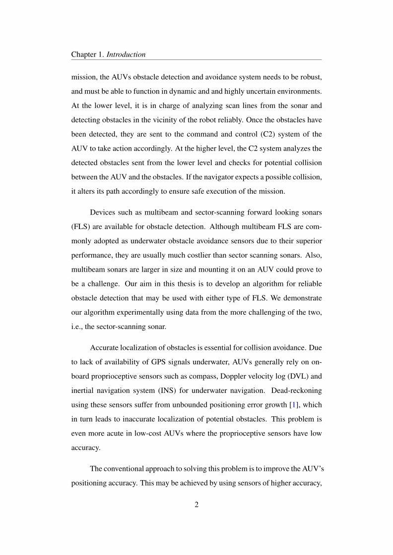
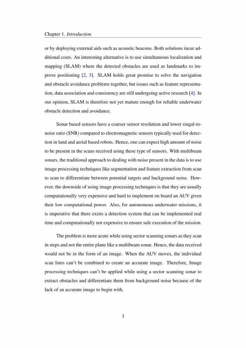
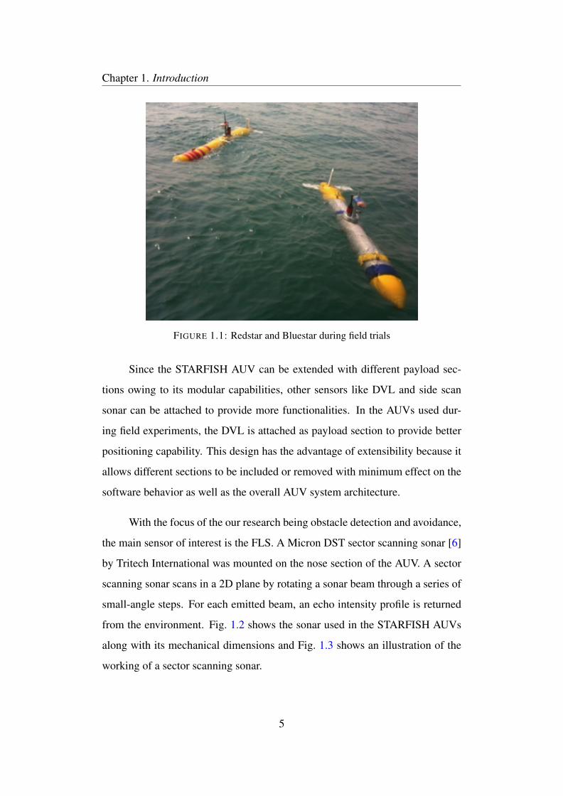
system architecture. Fig. 1.1 shows 2 STARFISH AUVs, namely Redstar and
Bluestar during one of the field trials at Selat Pauh, an anchorage off the coast
of Singapore.
Different sensors and actuators play an important role in the AUV to en-
sure the mission objectives are accomplished without compromising the safety
of the AUV. Hence, the AUV is equipped with a complete sensor suite and ac-
tuators. Firstly, the nose section is mounted with depth sensor, altitude sensor,
pressure sensor and a FLS. Then, the C2 section comprises of the compass and
GPS sensors for navigational purposes. It also hosts the main processing unit
(PC104 microprocessor) which is responsible for running the core software. Fi-
nally, the tail section is made of thrusters, fins and elevators which provide ma-
neuvering capabilities to the AUV. These 3 sections, namely Nose, C2 and Tail
is sufficient for basic operation of the AUV.
4
Chapter 1. Introduction
FIGURE 1.1: Redstar and Bluestar during field trials
Since the STARFISH AUV can be extended with different payload sec-
tions owing to its modular capabilities, other sensors like DVL and side scan
sonar can be attached to provide more functionalities. In the AUVs used dur-
ing field experiments, the DVL is attached as payload section to provide better
positioning capability. This design has the advantage of extensibility because it
allows different sections to be included or removed with minimum effect on the
software behavior as well as the overall AUV system architecture.
With the focus of the our research being obstacle detection and avoidance,
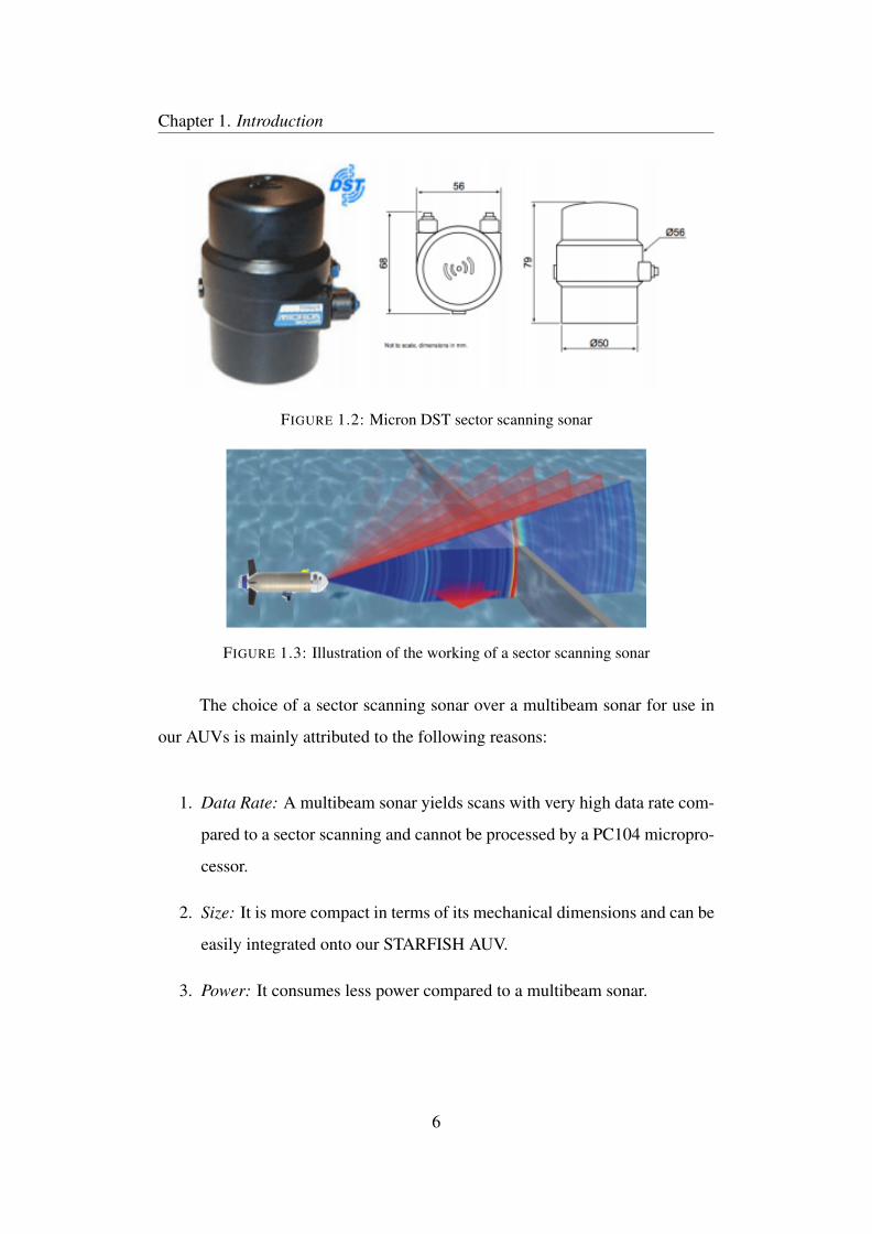
the main sensor of interest is the FLS. A Micron DST sector scanning sonar [6]
by Tritech International was mounted on the nose section of the AUV. A sector
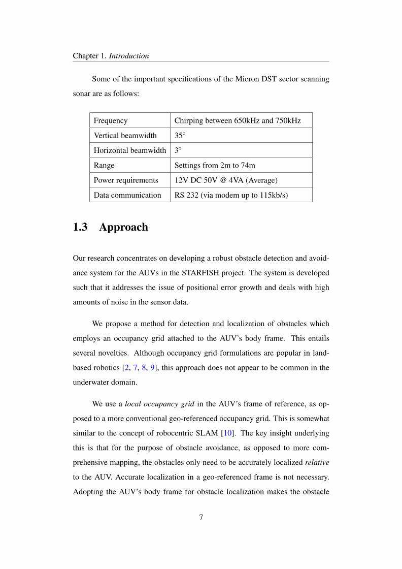
scanning sonar scans in a 2D plane by rotating a sonar beam through a series of
small-angle steps. For each emitted beam, an echo intensity profile is returned
from the environment. Fig. 1.2 shows the sonar used in the STARFISH AUVs
along with its mechanical dimensions and Fig. 1.3 shows an illustration of the
working of a sector scanning sonar.
5
Chapter 1. Introduction
FIGURE 1.2: Micron DST sector scanning sonar
FIGURE 1.3: Illustration of the working of a sector scanning sonar
The choice of a sector scanning sonar over a multibeam sonar for use in
our AUVs is mainly attributed to the following reasons:
1. Data Rate: A multibeam sonar yields scans with very high data rate com-
pared to a sector scanning and cannot be processed by a PC104 micropro-
cessor.
2. Size: It is more compact in terms of its mechanical dimensions and can be
easily integrated onto our STARFISH AUV.
3. Power: It consumes less power compared to a multibeam sonar.
6
Chapter 1. Introduction
Some of the important specifications of the Micron DST sector scanning
sonar are as follows:
Frequency Chirping between 650kHz and 750kHz
Vertical beamwidth 35◦
Horizontal beamwidth 3◦
Range Settings from 2m to 74m
Power requirements 12V DC 50V @ 4VA (Average)
Data communication RS 232 (via modem up to 115kb/s)
1.3 Approach
Our research concentrates on developing a robust obstacle detection and avoid-
ance system for the AUVs in the STARFISH project. The system is developed
such that it addresses the issue of positional error growth and deals with high
amounts of noise in the sensor data.
We propose a method for detection and localization of obstacles which
employs an occupancy grid attached to the AUV’s body frame. This entails
several novelties. Although occupancy grid formulations are popular in land-
based robotics [2, 7, 8, 9], this approach does not appear to be common in the
underwater domain.
We use a local occupancy grid in the AUV’s frame of reference, as op-
posed to a more conventional geo-referenced occupancy grid. This is somewhat
similar to the concept of robocentric SLAM [10]. The key insight underlying
this is that for the purpose of obstacle avoidance, as opposed to more com-
prehensive mapping, the obstacles only need to be accurately localized relative
to the AUV. Accurate localization in a geo-referenced frame is not necessary.
Adopting the AUV’s body frame for obstacle localization makes the obstacle
7
Chapter 1. Introduction
detection and avoidance performance less sensitive to the AUV’s positioning
error growth.
Also, our formulation incorporates motion uncertainties and sensor pa-
rameters such as false alarm rate and detection probability in a Bayesian frame-
work to deal with the high amounts of noise present in the sonar data. When
the AUV moves, the obstacles “move” in the AUV’s body frame in a predictable
way. Our motion model updates the occupancy probabilities from the estimated
translational and rotational motion. When a sonar measurement becomes avail-
able, the occupancy probabilities are updated using a Bayesian measurement
model that integrates new information from the measurement into the belief rep-
resented by the occupancy grid.
Finally, the occupancy grid is used to determine the location of nearby
obstacles. If these obstacles pose a threat of collision, the AUV’s C2 system
takes evasive maneuvers.
1.4 Thesis Layout
This thesis is organized as follows. Chapter 2 provides a brief discussion of
related works in underwater obstacle detection and avoidance for AUVs. Chap-
ter 3 presents the technical approach involved in detecting an obstacle and a
novel method to generate a local occupancy grid. Chapter 4 presents experimen-
tal results for detection of various targets in a lake and sea environment. Chap-
ters 5 discusses the Command and Control (C2) system used in the STARFISH
AUV and how the avoidance sub-system is incorporated into it. Chapter 6
presents results from simulations and lake experiments to demonstrate the avoid-
ance behavior of a STARFISH AUV. Finally, Chapter 7 concludes the thesis and
makes suggestions for future work.
8
Chapter 2
Background
Developing an underwater obstacle detection and avoidance mechanism for an
autonomous and remotely operated underwater robotic systems is a challenging
task for researchers. The system needs to be robust and capable of handling
uncertainties that are likely to arise during an autonomous underwater mission in
hazardous environments. Over the years, many obstacle detection and avoidance
techniques have been designed and implemented on autonomous underwater,
ground and aerial robotic system.
Most land or aerial based robots tend to use LASER sensors for obstacle
detection which have higher SNR and better resolution. Hence, one can expect
better performance in terms of detection capabilities using a LASER sensor.
However, underwater robots are limited to the use of sonar sensors which have
low SNR and coarser resolution. Hence, typical scans received from sonar sen-
sors have high amounts of noise present in them. Researchers have used image
processing techniques like segmentation and feature extraction on these scans
to differentiate obstacles from background noise and detect them. Once an ob-
stacle has been detected consistently, they avoid it if there is a possibility of a
collision.
9
Chapter 2. Background
Underwater robots also face the problem of accurate localization since
GPS signals are not available underwater. Hence, they suffer an unbounded
positional error growth. As a result, detected obstacles cannot be localized ac-
curately with respect to the global frame because of the existing positional error
of the AUV. Researchers have used SLAM based techniques to help localize the
AUV and hence reduce the positional error growth of the robot. In doing so,
they build a global map with various features and obstacles with some amount
of uncertainty in their position. After generating a global map, if the AUV
senses a potential collision with one of the obstacles during a mission, the AUV
then plans an evasive maneuver such that the clearance radius is greater than the
uncertainty in the position of the obstacle.
2.1 Image Processing Techniques
The basis of a sonar detection problem is to decide from the return of a sonar
ping whether an obstacle is present on not. In a sonar measurement, the repre-
sentation of an object is ideally a signal reading with an intensity higher than
the background. However, sonar measurements are contaminated with high
amounts of noise due to various sources (i.e. thermal noise, acoustic noise and
multipath reverberations).
In [11], Hordur et al process scan lines (sector scanning sonar) as such
and do not buffer them and process as an image. However, the techniques used
on individual scan lines are similar to what would be applied on an image. The
authors generate a smoothed histogram of the data and look at the modes of the
distribution. A threshold between the second largest mode and the first largest
mode is then chosen. Using this selected value, the sonar return data is thresh-
olded and targets are considered to be present in the regions where the intensities
are greater than the threshold. The authors also compare the current scan with
10
Chapter 2. Background
the previous scan to ensure rejection of spurious returns due to turbulent water.
Experimental results of detection and avoidance using a Autonomous Surface
Vehicle (ASV) are presented to substantiate the working of their technique.
Quidu et al [12] use a multibeam sonar to detect obstacles and avoid them.
Hence, instead of receiving a single scan line from a particular bearing, a com-
plete scan over the entire sector is obtained. As a result, image processing tech-
niques are applied on the scans received. Strong intensity targets are detected
by simply thresholding the image. The threshold value used is typically 75%
of the maximum intensity in the image. Detection of medium strength targets
is slightly involved. The authors first pass the image through a low-pass filter.
Following this, a two step filtering procedure is applied on the image. First,
an average filter is applied on the segmented image to filter noise and lower
false alarm rate. Then the shadow regions are removed from the filtered image.
Finally, the medium intensity targets can be detected in the same way as strong
intensity targets by thresholding the filtered image. Once an obstacle is detected,
a track is initialized and confirmed if it can be consistently detected over 3 scans.
If not, the corresponding track is killed. If the tracked obstacle poses a threat of
collision, the AUV uses a potential field approach [13] to avoid it.
Elsewhere, Teo et al [14] also employed image processing techniques to
extract potential obstacles from the images received using a multibeam sonar
on the MEREDITH AUV, while Horner et al [15] used a sector scanning sonar
to collect a sequential set of scan lines to create an image. Image processing
techniques were then applied on this image. It should be noted that an image
created by collecting scan lines over the entire sector as the AUV moves would
not be accurate. Some form of motion compensation needs to be applied on the
individual scan lines to create an accurate image. Furthermore, such an approach
reduces the real time nature of the detection procedure.
11
Chapter 2. Background
From literature, it can be observed that majority of obstacle detection and
avoidance algorithms developed for mobile underwater robots use image pro-
cessing techniques. These techniques have also demonstrated reliability and
extendability from a sector scanning sonar to a multibeam sonar. Also, this
approach usually localizes obstacles accurately with respect to the AUV since
the scans received are in the AUVs frame of reference. This circumvents the
problem of positional error growth of the AUV in the global frame which in
turn leads to inaccurate localization of obstacles in the global frame. Finally,
this technique has been proved to be capable of handling various situations and
uncertainties in a highly dynamic environment.
However, the authors in [12, 16] acknowledge that the image processing
techniques used in their respective works are computationally expensive. Hence,
their experimental data were processed offline owning to limited computational
resources available on board their respective AUVs. Also, applying image pro-
cessing techniques on images created using a sector scanning sonar is no longer
a real time approach to detection. In addition to that, some image process-
ing techniques use feature extraction methods to detect obstacles [14, 16, 17].
However, it is often very difficult to extract reliable features from underwater
environments using FLS data, especially when a sector scanning sonar is used.
Fig. 2.1 shows an unprocessed image created while scanning a coral reef
using a sector scanning sonar on board the STARFISH AUV. It can be seen that
are no distinct features in the image and hence feature extraction techniques are
bound to fail in underwater environments which lack distinct features.
12

Chapter 2. Background
−40 −20 0 20 400
10
20
30
40
50
x (metres)
y (
me
tre
s)
0
50
100
150
200
250
FIGURE 2.1: Raw scan of a coral reef using a sector scanning sonar
2.2 SLAM Techniques
Researchers have also adopted SLAM based approaches [3, 18] to obstacle de-
tection and avoidance in underwater environments. Lack of GPS signals in un-
derwater environments leads to increasing positional uncertainty of the AUV.
SLAM techniques essentially builds a global map by adding detected features
into it. It then uses these detected features as landmarks to improve the error in
the robot’s position. Reducing the AUVs positional error in turn helps in localiz-
ing obstacles more accurately with respect to the global frame. Hence, obstacles
that pose a threat in terms of collision can be avoided safely during a mission.
Leedekerken et al [3] used an extended Kalman Filter (EKF) as the main
tool to carry out SLAM. The authors use an EKF to estimate the dynamic pa-
rameters of the robot’s state as well as the static state parameters of the observed
features. However, in large environments, as the number of features grows, so
13
Chapter 2. Background
does the complexity of the state estimator. To tackle this problem, the authors
propose the use of local submaps. This results in an accurate local map but
sacrifices the accuracy of the global map for stability and bounded complexity.
Hence as long as the AUV traverses within a particular local map, accurate local-
ization and hence avoidance in possible. However path planning for avoidance
in the global map could prove to be hazardous because of the error associated
between different local maps which constitute the global map. In [18], Ribas et
al also present a procedure to build and maintain a sequence of local maps and
then posteriorly recover the full global map.
Feature extraction forms a key component in SLAM based techniques.
In [19], Majumder et al fuse data from sonar and vision sensors following which
feature extraction is performed on the fused data. The posterior distribution
of the map is updated using a Bayesian approach for each identified feature.
However, successful extraction of features is only possible if the features are
distinct and can be associated with some form of geometrical representation
(For e.g., walls can be represented by straight lines). Underwater environments
generally lack such features and hence map building using feature extraction
techniques may not be a reliable approach.
SLAM holds great promise to solve the navigation and obstacle avoidance
problems together, but issues such as feature representation, data association and
consistency are still undergoing active research [4]. Furthermore, the existence
of distinct features is necessary for robust performance of SLAM. However,
underwater environments often lack such distinct features, as shown in Fig. 2.1,
and hence a typical SLAM approach is likely to fail. In our opinion, SLAM is
therefore not yet mature enough for reliable underwater obstacle detection and
avoidance.
14
Chapter 2. Background
2.3 Occupancy Grids
Occupancy grids are better equipped to deal with noisy data since they associate
a probability of occupancy to every cell on the grid instead of using a hard
threshold on the intensity value to indicate a detection. Also, we believe that the
occupancy grid approach is particularly suitable for underwater robotics because
of the difficulty involved in extracting reliable features which are needed for both
image processing and SLAM based techniques.
In literature, there are two types of occupancy grids that can be used for
the purpose of obstacle detection and navigation. They are:
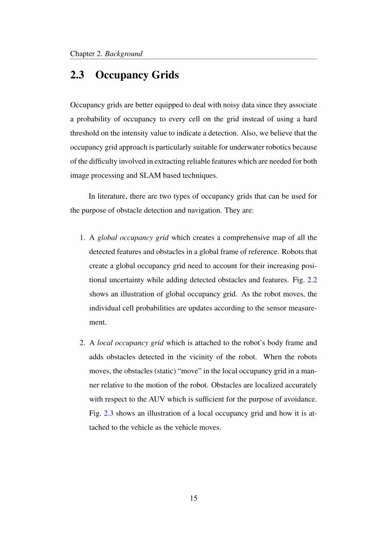
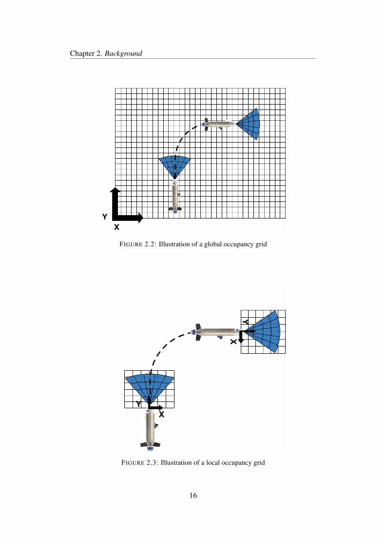
1. A global occupancy grid which creates a comprehensive map of all the
detected features and obstacles in a global frame of reference. Robots that
create a global occupancy grid need to account for their increasing posi-
tional uncertainty while adding detected obstacles and features. Fig. 2.2
shows an illustration of global occupancy grid. As the robot moves, the
individual cell probabilities are updates according to the sensor measure-
ment.
2. A local occupancy grid which is attached to the robot’s body frame and
adds obstacles detected in the vicinity of the robot. When the robots
moves, the obstacles (static) “move” in the local occupancy grid in a man-
ner relative to the motion of the robot. Obstacles are localized accurately
with respect to the AUV which is sufficient for the purpose of avoidance.
Fig. 2.3 shows an illustration of a local occupancy grid and how it is at-
tached to the vehicle as the vehicle moves.
15
Chapter 2. Background
X
Y
FIGURE 2.2: Illustration of a global occupancy grid
Y
X
Y
X
FIGURE 2.3: Illustration of a local occupancy grid
16
Chapter 2. Background
In [7, 8], the authors provide a mathematical formulation to generate a
global occupancy grid using sonar data for the purpose of navigation while tak-
ing into account the increasing error in the position of the robot. Local oc-
cupancy grids have also been used for the purpose of navigation and obstacle
avoidance. While Fulgenzi et al in [20] used the same to navigate safely in the
presence of obstacles in a land environment, Marlow et al in [21] used local
occupancy grids in an aerial environment to avoid obstacles.
Although occupancy grid formulations are popular in land and aerial based
robotics [2, 7, 8, 9, 20, 21], this approach does not appear to be common in the
underwater domain. Existing publications on occupancy grids for FLS, such as
[22] and [23], present results from a controlled environment and under static
conditions. However, to the best of our knowledge, there has been no exper-
imental results showing obstacle detection and avoidance with the AUV in a
dynamic state using occupancy grids, local or global, in an underwater environ-
ment.
Even though there exists techniques for obstacle detection and avoidance
using local occupancy grids in land and aerial environments, they cannot be
directly applied in an underwater environment. Hence, our main contribution
would be the mathematical formulation to generate a local occupancy grid for
obstacle detection and avoidance in an underwater environment.
2.4 Summary
Image processing and SLAM based techniques can only solve either one of the
problem faced by AUVs with respect to obstacle detection and avoidance. Also,
the works discussed in Sections 2.1 to 2.3 expose some shortcomings and limi-
tations. Contrary to the works discussed in Sections 2.1 to 2.3, our proposed ap-
proach tackles both the mentioned problems and addresses the shortcomings and
17
Chapter 2. Background
limitations as well. The use of a local occupancy helps in localizing obstacles
accurately with respect to the AUV and is sufficient for the purpose of avoid-
ance. It also circumvents the problem of positional uncertainty of the AUV in
the global frame which in turn leads to inaccurate localization of obstacles in the
global frame. Furthermore, a probabilistic framework which takes into account
the detection probabilities and false alarm rate to deal with the high amount of
noise in the scans is proposed. The aim is to develop a robust obstacle detection
and avoidance technique which can be implemented onboard an AUV.
18
Chapter 3
Underwater Obstacle Detection
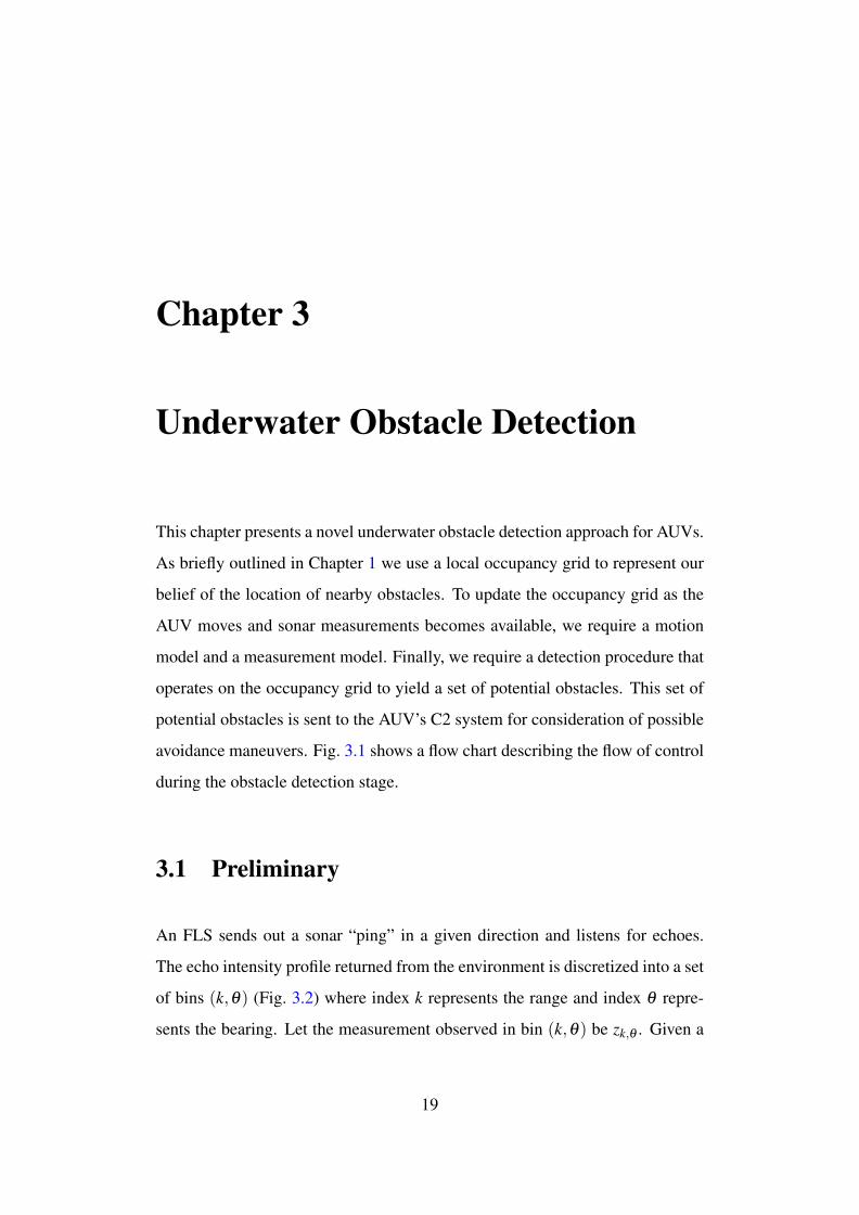
This chapter presents a novel underwater obstacle detection approach for AUVs.
As briefly outlined in Chapter 1 we use a local occupancy grid to represent our
belief of the location of nearby obstacles. To update the occupancy grid as the
AUV moves and sonar measurements becomes available, we require a motion
model and a measurement model. Finally, we require a detection procedure that
operates on the occupancy grid to yield a set of potential obstacles. This set of
potential obstacles is sent to the AUV’s C2 system for consideration of possible
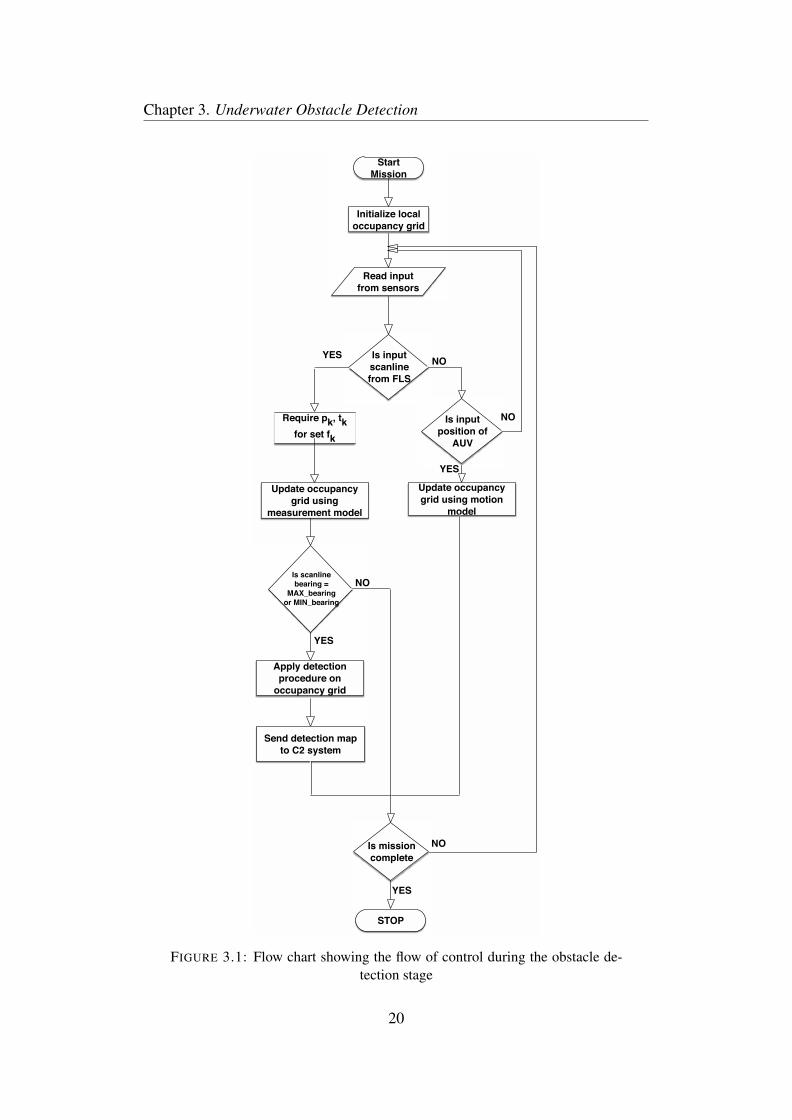
avoidance maneuvers. Fig. 3.1 shows a flow chart describing the flow of control
during the obstacle detection stage.
3.1 Preliminary
An FLS sends out a sonar “ping” in a given direction and listens for echoes.
The echo intensity profile returned from the environment is discretized into a set
of bins (k,θ) (Fig. 3.2) where index k represents the range and index θ repre-
sents the bearing. Let the measurement observed in bin (k,θ) be zk,θ . Given a
19
Chapter 3. Underwater Obstacle Detection
Is scanline
bearing =
MAX_bearing
or MIN_bearing
Start
Mission
Require pk, tk
for set fk
Read input
from sensors
Initialize local
occupancy grid
Update occupancy
grid using
measurement model
Update occupancy
grid using motion
model
Is input
scanline
from FLS
YESNO
Is input
position of
AUV
YES
NO
Apply detection
procedure on
occupancy grid
YES
NO
Send detection map
to C2 system
Is mission
complete
YES
STOP
NO
FIGURE 3.1: Flow chart showing the flow of control during the obstacle de-tection stage
20
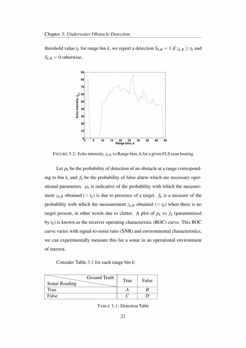
Chapter 3. Underwater Obstacle Detection
threshold value tk for range bin k, we report a detection Sk,θ = 1 if zk,θ ≥ tk and
Sk,θ = 0 otherwise.
0 5 10 15 20 25 30 35 40 450
10
20
30
40
50
60
70
80
90
Range bins, k
Ech
o I
nte
nsit
y, z k
,θ
FIGURE 3.2: Echo intensity, zk,θ vs Range bins, k for a given FLS scan bearing
Let pk be the probability of detection of an obstacle at a range correspond-
ing to bin k, and fk be the probability of false alarm which are necessary oper-
ational parameters. pk is indicative of the probability with which the measure-
ment zk,θ obtained (> tk) is due to presence of a target. fk is a measure of the
probability with which the measurement zk,θ obtained (> tk) when there is no
target present, in other words due to clutter. A plot of pk vs fk (parametrized
by tk) is known as the receiver operating characteristic (ROC) curve. This ROC
curve varies with signal-to-noise ratio (SNR) and environmental characteristics;
we can experimentally measure this for a sonar in an operational environment
of interest.
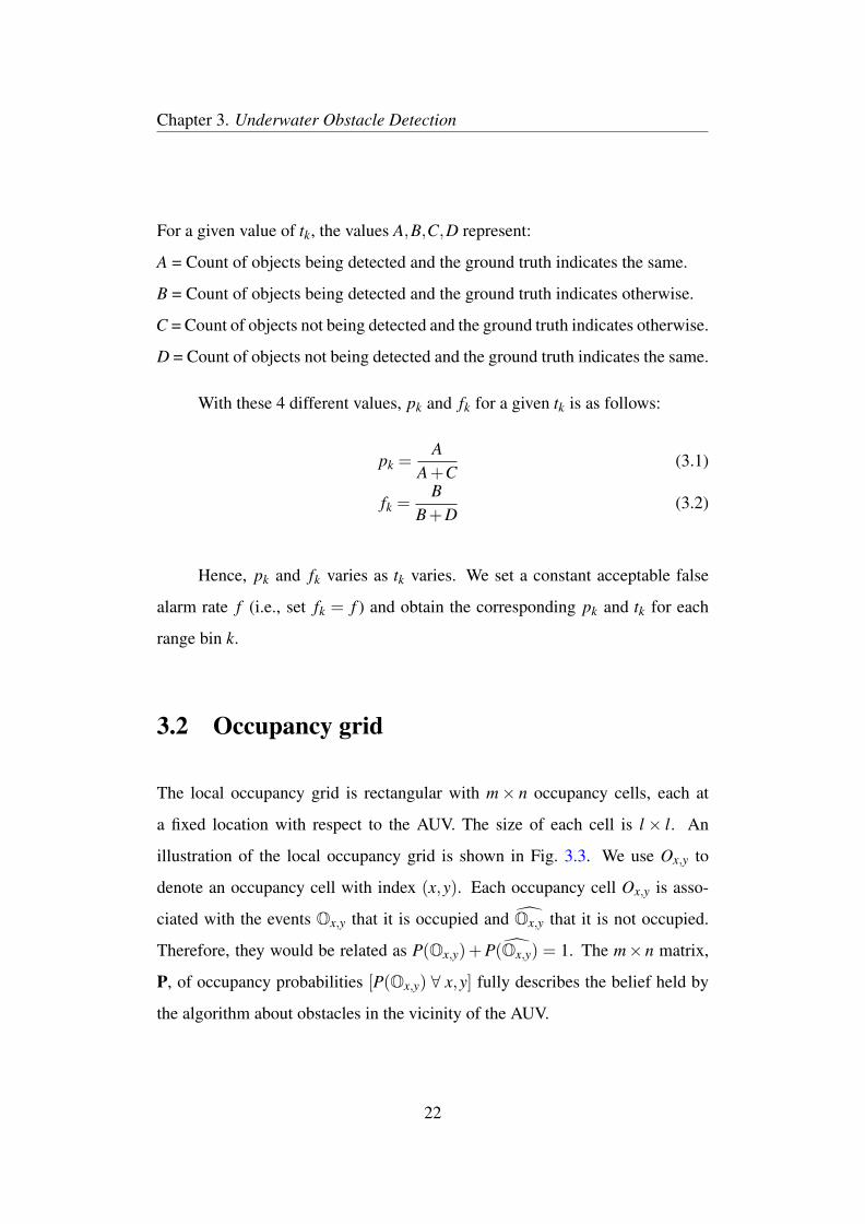
Consider Table 3.1 for each range bin k:
hhhhhhhhhhhhhhhhhhSonar ReadingGround Truth
True False
True A BFalse C D
TABLE 3.1: Detection Table
21
Chapter 3. Underwater Obstacle Detection
For a given value of tk, the values A,B,C,D represent:
A = Count of objects being detected and the ground truth indicates the same.
B = Count of objects being detected and the ground truth indicates otherwise.
C = Count of objects not being detected and the ground truth indicates otherwise.
D = Count of objects not being detected and the ground truth indicates the same.
With these 4 different values, pk and fk for a given tk is as follows:
pk =A
A+C(3.1)
fk =B
B+D(3.2)
Hence, pk and fk varies as tk varies. We set a constant acceptable false
alarm rate f (i.e., set fk = f ) and obtain the corresponding pk and tk for each
range bin k.
3.2 Occupancy grid
The local occupancy grid is rectangular with m× n occupancy cells, each at
a fixed location with respect to the AUV. The size of each cell is l × l. An
illustration of the local occupancy grid is shown in Fig. 3.3. We use Ox,y to
denote an occupancy cell with index (x,y). Each occupancy cell Ox,y is asso-
ciated with the events Ox,y that it is occupied and Ox,y that it is not occupied.
Therefore, they would be related as P(Ox,y)+P(Ox,y) = 1. The m× n matrix,
P, of occupancy probabilities [P(Ox,y) ∀ x,y] fully describes the belief held by
the algorithm about obstacles in the vicinity of the AUV.
22
Chapter 3. Underwater Obstacle Detection
FIGURE 3.3: Illustration of local occupancy grid attached to the AUV and itssensor frame (blue color)
3.3 Measurement Model
When a measurement becomes available, the occupancy grid serves as a Bayesian
prior. Depending on whether Sk,θ = 1 (zk,θ ≥ tk) or Sk,θ = 0 (zk,θ < tk), the oc-
cupancy cells are updated to the posterior probabilities using Bayes’ rule and
the probabilities pk and f obtained as per Section 3.1.
Fig. 3.4 shows the overlap between occupancy cells and a particular range
bin. Let the region of overlap between any range bin (k,θ) and any occupancy
cell Ox,y be denoted by Ox,yk,θ . Also, let Ox,y
k,θ denote the event that the region
Ox,yk,θ be occupied. We define our measurement model such that Sk,θ = 1 will
be observed when a target is present in any one of the overlapping regions Ox,yk,θ
with a probability equal to the probability of detection. This give rise to four
23
Chapter 3. Underwater Obstacle Detection
possible combination of events as follows:
P(Sk,θ = 1|Ox,yk,θ ) = pk (3.3)
P(Sk,θ = 1|Ox,yk,θ ) = f (3.4)
P(Sk,θ = 0|Ox,yk,θ ) = 1− pk (3.5)
P(Sk,θ = 0|Ox,yk,θ ) = 1− f (3.6)
Let the area of overlap between range bin (k,θ) and occupancy cell Ox,y
be vx,yk,θ and the area of an occupancy cell be denoted by A(Ox,y). Now the events
Ox,yk,θ and Ox,y are related as follows:
P(Ox,yk,θ |Ox,y) =
vx,yk,θ
A(Ox,y)= ax,y
k,θ (3.7)
P(Ox,yk,θ |Ox,y) = 1−ax,y
k,θ (3.8)
P(Ox,yk,θ |Ox,y) = 1 (3.9)
P(Ox,yk,θ |Ox,y) = 0 (3.10)
Occupancy cells
Sensor cell
v4
v2
v1
v3
O4O3
O2O1
FIGURE 3.4: Illustration of overlap between occupancy cells and a sensor cell.The area of overlap between a range bin and O{i}, is v{i} where i ∈ {1, . . . ,4}.
24
Chapter 3. Underwater Obstacle Detection
Finally, the map is updated for the two possible cases corresponding to
Sk,θ = 1 or Sk,θ = 0 as follows:
Case 1: Whenever the measurement obtained is such that Sk,θ = 1 (zk,θ ≥ tk),
the occupancy cell Ox,y is updated as follows:
P(Ox,y|Sk,θ = 1) =P(Sk,θ = 1|Ox,y)P(Ox,y)
P(Sk,θ = 1)(3.11)
P(Sk,θ = 1|Ox,y) = 1−P(Sk,θ = 0|Ox,y) (3.12)
P(Sk,θ = 0|Ox,y) =m
∏i=1
n
∏j=1
{ Oi, j
∑Oi, j
Oi, jk,θ
∑Oi, j
k,θ
P(Sk,θ = 0|Oi, jk,θ )P(O
i, jk,θ |Oi, j)P(Oi, j|Ox,y)
}
=m
∏i=1
n
∏j=1
{P(Sk,θ = 0|Oi, j
k,θ )P(Oi, jk,θ |Oi, j)P(Oi, j|Ox,y)
+ P(Sk,θ = 0|Oi, jk,θ )P(O
i, jk,θ |Oi, j)P(Oi, j|Ox,y)
+ P(Sk,θ = 0|Oi, jk,θ )P(O
i, jk,θ |Oi, j)P(Oi, j|Ox,y)
+ P(Sk,θ = 0|Oi, jk,θ )P(O
i, jk,θ |Oi, j)P(Oi, j|Ox,y)
}(3.13)
=(
1− f +ax,yk,θ ( f − pk)
){ m
∏i=1
n
∏j=1
{(1− f +ax,y
k,θ ( f − pk))
P(Oi, j)
+ (1− f )P(Oi, j)
}}∀(i, j) 6= (x,y) (3.14)
P(Sk,θ = 1) = 1−P(Sk,θ = 0) (3.15)
P(Sk,θ = 0) =m
∏i=1
n
∏j=1
{ Oi, j
∑Oi, j
Oi, jk,θ
∑Oi, j
k,θ
P(Sk,θ = 0|Oi, jk,θ )P(O
i, jk,θ |Oi, j)P(Oi, j)
}
P(Sk,θ = 0) =m
∏i=1
n
∏j=1
{(1− f +ax,y
k,θ ( f − pk))
P(Oi, j)
+ (1− f )P(Oi, j)
}(3.16)
where P(Sk,θ = 1|Ox,y) denotes the likelihood of getting a measurement zk,θ ≥
tk from range bin (k,θ) given Ox,y is already occupied and P(Sk,θ = 1) is the
normalizing constant. ai, jk,θ becomes zero when the occupancy cell is far away
from the range bin (k,θ). Hence, we only update the probabilities within the
25
Chapter 3. Underwater Obstacle Detection
neighborhood of r× r occupancy cells that enclose range bin (k,θ). Also, while
updating each occupancy cell Ox,y in the r× r neighborhood, only the other
occupancy cells Oi, j in the same neighborhood will be involved.
It should be noted that for the case when Sk,θ = 1, all possible combina-
tions of detections and/or false alarms from all possible combinations of over-
lapping occupancy cells need to be considered. Hence calculating P(Sk,θ = 1)
becomes rather involved. But Sk,θ = 0 occurs only when a detection was missed
or there was no target present in all the overlapping cells for which the probabil-
ity can be calculated in a straightforward manner. Following which, P(Sk,θ = 1)
can be calculated by taking the compliment of P(Sk,θ = 0).
Case 2: When the measurement obtained is such that Sk,θ = 0 (zk,θ < tk), the
occupancy cell Ox,y is updated is a slightly different manner.
P(Ox,y|Sk,θ = 0) =P(Sk,θ = 0|Ox,y)P(Ox,y)
P(Sk,θ = 0)(3.17)
where P(Sk,θ = 0|Ox,y) denotes the likelihood of getting a measurement zk < tk
from a range bin (k,θ) given Ox,y is occupied. It can be obtained as per Eq. 3.13
and the normalizing constant, P(Sk,θ = 0), can be obtained from Eq. 3.16.
The implicit assumption made in the formulation is that the probabilities
with which the cells are occupied are independent from one another.
3.4 Motion model
The motion model takes into account the translation and the rotational motion
of the AUV and tracks the probabilities of the occupancy cells accordingly. It is
defined such that the translational motion and rotational motion are decoupled
from one another.
26
Chapter 3. Underwater Obstacle Detection
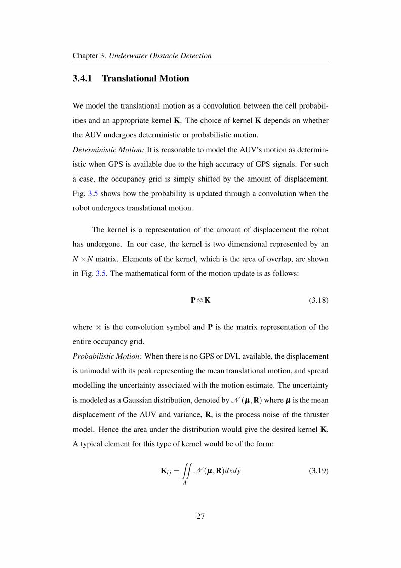
3.4.1 Translational Motion
We model the translational motion as a convolution between the cell probabil-
ities and an appropriate kernel K. The choice of kernel K depends on whether
the AUV undergoes deterministic or probabilistic motion.
Deterministic Motion: It is reasonable to model the AUV’s motion as determin-
istic when GPS is available due to the high accuracy of GPS signals. For such
a case, the occupancy grid is simply shifted by the amount of displacement.
Fig. 3.5 shows how the probability is updated through a convolution when the
robot undergoes translational motion.
The kernel is a representation of the amount of displacement the robot
has undergone. In our case, the kernel is two dimensional represented by an
N×N matrix. Elements of the kernel, which is the area of overlap, are shown
in Fig. 3.5. The mathematical form of the motion update is as follows:
P⊗K (3.18)
where ⊗ is the convolution symbol and P is the matrix representation of the
entire occupancy grid.
Probabilistic Motion: When there is no GPS or DVL available, the displacement
is unimodal with its peak representing the mean translational motion, and spread
modelling the uncertainty associated with the motion estimate. The uncertainty
is modeled as a Gaussian distribution, denoted by N (µµµ,R) where µµµ is the mean
displacement of the AUV and variance, R, is the process noise of the thruster
model. Hence the area under the distribution would give the desired kernel K.
A typical element for this type of kernel would be of the form:
Ki j =∫∫A
N (µµµ,R)dxdy (3.19)
27
Chapter 3. Underwater Obstacle Detection
The integral is evaluated over the region of the distribution represented by the
element Ki j. The grid is updated using Eq. 3.18.
Δx
Δy
O-5
O-neww4
w5
w8w7
w4 = (1-Δy)* Δx
w5 = (1-Δx)*(1-Δy)
w7 = Δx* Δy
w8 = (1-Δx)* Δy
P(O-new) = w4*P(O4) + w5*P(O-5) + w7*P(O-6) + w8*P(O-8)
Occupancy Cell
Neighbouring Occupancy Cells after translation
FIGURE 3.5: Illustration of overlap of neighboring occupancy cells after un-dergoing translation with a particular occupancy cell. The area of overlap be-
tween O-new and O-{i}, is w-{i} where i ∈ {4,5,7 and 8}.
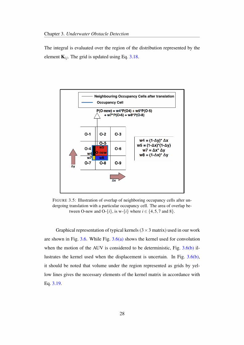
Graphical representation of typical kernels (3×3 matrix) used in our work
are shown in Fig. 3.6. While Fig. 3.6(a) shows the kernel used for convolution
when the motion of the AUV is considered to be deterministic, Fig. 3.6(b) il-
lustrates the kernel used when the displacement is uncertain. In Fig. 3.6(b),
it should be noted that volume under the region represented as grids by yel-
low lines gives the necessary elements of the kernel matrix in accordance with
Eq. 3.19.
28
Chapter 3. Underwater Obstacle Detection
0
1
2
3 3
2
1
0
x y
(1- Δx)*Δy
(1- Δx)*(1- Δy)
Δx*Δy
Δx*(1-Δy)
(a) Deterministic Kernel
0
1
2
3
0
1
2
3
x y
(b) Probabilistic Kernel
FIGURE 3.6: Graphical Representation of Kernels
29
Chapter 3. Underwater Obstacle Detection
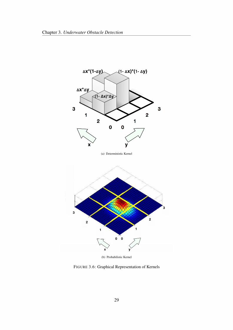
3.4.2 Rotational Motion:
We model the rotational motion of the AUV as deterministic. This is because
the accuracy of the compass used is quite high. To avoid rounding errors, we
accumulate changes in heading until they reach ±1◦. The area of overlap of
rotated neighboring occupancy cells O′x−i,y− j ∀ i, j ∈ {−1,0,1}with a particular
occupancy cell Ox,y is calculated. Then the new probability of occupancy is
updated as:
P(Ox,y) = ∑i
∑j
wx−i,y− jx,y P(O′x−i,y− j) (3.20)
where wx−i,y− jx,y is the ratio of the area of overlap between occupancy cell O′x−i,y− j
and Ox,y and the area of occupancy cell Ox,y. Fig. 3.7 shows how the probability
is updated in the presence of rotation.
FIGURE 3.7: Illustration of overlap of neighboring occupancy cells after un-dergoing rotation with a particular occupancy cell. The area of overlap be-
tween O-new and O-{i}, is w-{i} where i ∈ {2,4,5,6 and 8}.
30
Chapter 3. Underwater Obstacle Detection
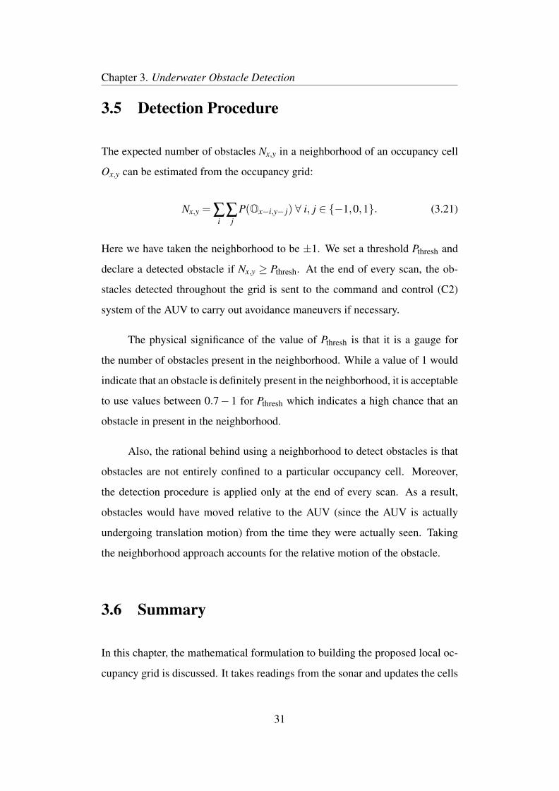
3.5 Detection Procedure
The expected number of obstacles Nx,y in a neighborhood of an occupancy cell
Ox,y can be estimated from the occupancy grid:
Nx,y = ∑i
∑j
P(Ox−i,y− j) ∀ i, j ∈ {−1,0,1}. (3.21)
Here we have taken the neighborhood to be ±1. We set a threshold Pthresh and
declare a detected obstacle if Nx,y ≥ Pthresh. At the end of every scan, the ob-
stacles detected throughout the grid is sent to the command and control (C2)
system of the AUV to carry out avoidance maneuvers if necessary.
The physical significance of the value of Pthresh is that it is a gauge for
the number of obstacles present in the neighborhood. While a value of 1 would
indicate that an obstacle is definitely present in the neighborhood, it is acceptable
to use values between 0.7− 1 for Pthresh which indicates a high chance that an
obstacle in present in the neighborhood.
Also, the rational behind using a neighborhood to detect obstacles is that
obstacles are not entirely confined to a particular occupancy cell. Moreover,
the detection procedure is applied only at the end of every scan. As a result,
obstacles would have moved relative to the AUV (since the AUV is actually
undergoing translation motion) from the time they were actually seen. Taking
the neighborhood approach accounts for the relative motion of the obstacle.
3.6 Summary
In this chapter, the mathematical formulation to building the proposed local oc-
cupancy grid is discussed. It takes readings from the sonar and updates the cells
31
Chapter 3. Underwater Obstacle Detection
accordingly. With the use of a sector scanning sonar, we can expect not all occu-
pancy cells to be updated regularly. It could take a while before some occupancy
cells are updated through the measurement model. Hence, in order to estimate
the probabilities in the absence of sonar readings, we use a motion model. It can
also be thought of as a form of motion compensation for detected targets.
Finally, we propose a detection procedure which acts on the grid at the
end of every scan. It yields regions in the local frame where the potential of
finding obstacles are quite high. These regions are then sent to the C2 system of
the AUV to take necessary actions.
32
Chapter 4
Results on Obstacle Detection
4.1 Experimental Setup
Experiments were conducted at Pandan reservoir in Singapore and also in the
sea off the coast of Singapore. For both sets of experiments, we used a Micron
DST sector scanning sonar [6] integrated on our STARFISH AUV [5].
During the Pandan experiment, the mission was planned such that the
AUV would be operating near some static buoys and the reservoir’s embank-
ments. The sonar was configured for 50 m operating range with 44 bins and 90◦
scan sector. The mission was executed with the AUV maintaining a constant
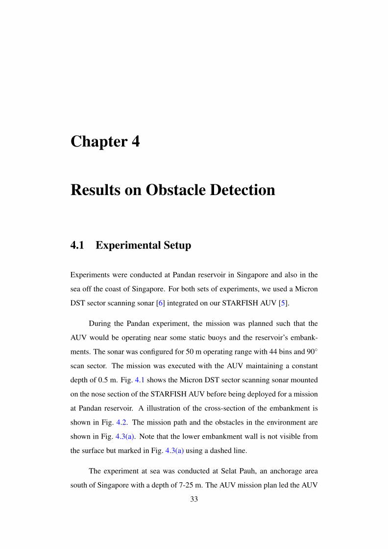
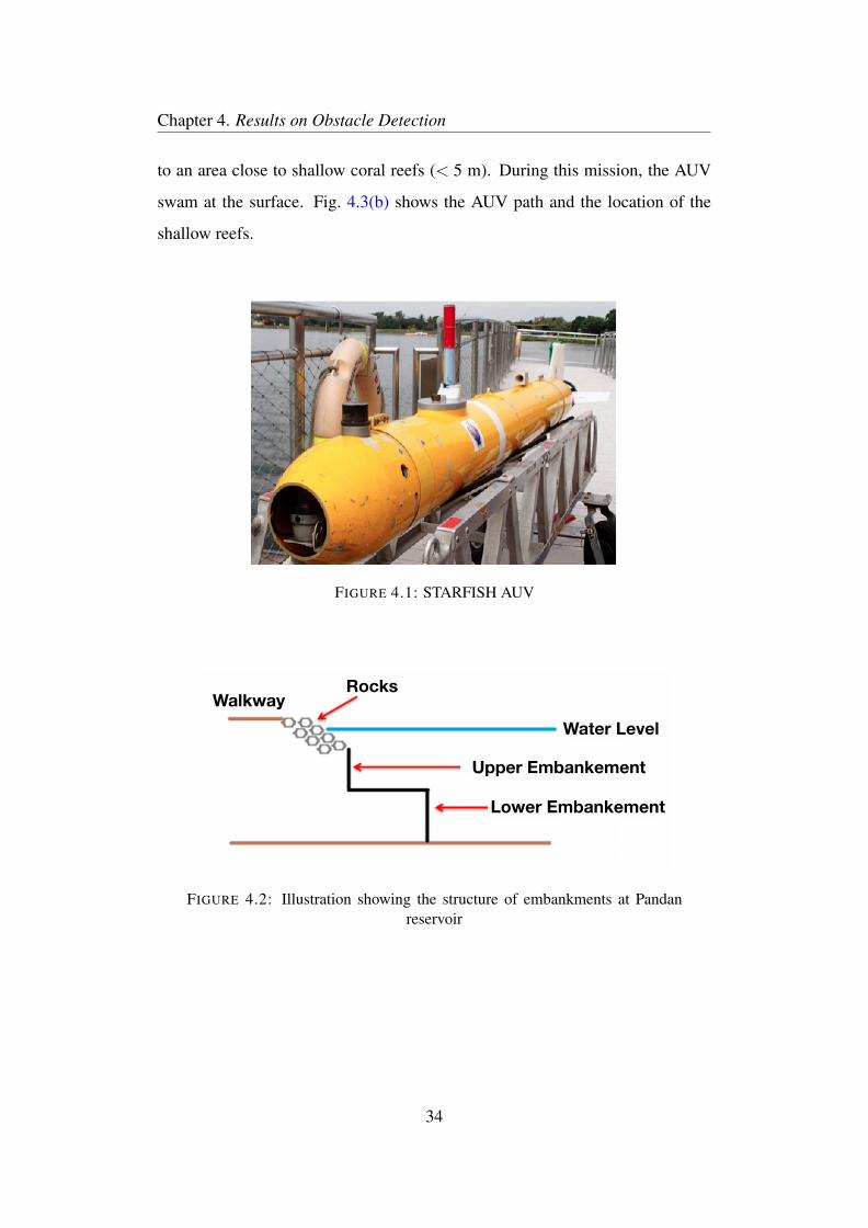
depth of 0.5 m. Fig. 4.1 shows the Micron DST sector scanning sonar mounted
on the nose section of the STARFISH AUV before being deployed for a mission
at Pandan reservoir. A illustration of the cross-section of the embankment is
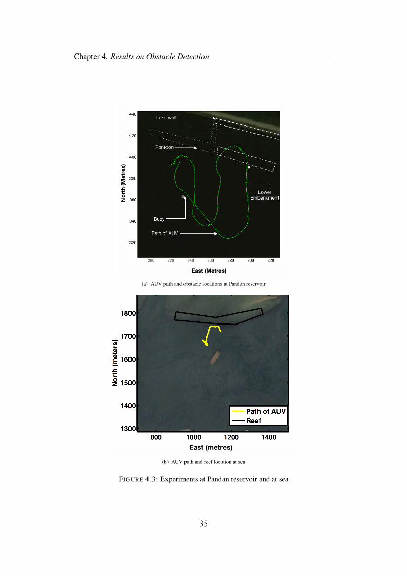
shown in Fig. 4.2. The mission path and the obstacles in the environment are
shown in Fig. 4.3(a). Note that the lower embankment wall is not visible from
the surface but marked in Fig. 4.3(a) using a dashed line.
The experiment at sea was conducted at Selat Pauh, an anchorage area
south of Singapore with a depth of 7-25 m. The AUV mission plan led the AUV
33
Chapter 4. Results on Obstacle Detection
to an area close to shallow coral reefs (< 5 m). During this mission, the AUV
swam at the surface. Fig. 4.3(b) shows the AUV path and the location of the
shallow reefs.
FIGURE 4.1: STARFISH AUV
Rocks
Water Level
Walkway
Upper Embankement
Lower Embankement
FIGURE 4.2: Illustration showing the structure of embankments at Pandanreservoir
34
Chapter 4. Results on Obstacle Detection
East (Metres)
No
rth
(M
etr
es)
(a) AUV path and obstacle locations at Pandan reservoir
East (metres)
(b) AUV path and reef location at sea
FIGURE 4.3: Experiments at Pandan reservoir and at sea
35
Chapter 4. Results on Obstacle Detection
4.2 Noise Distribution
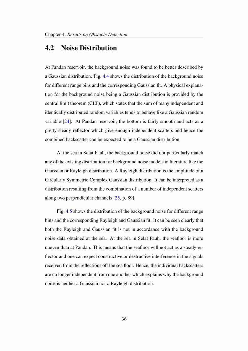
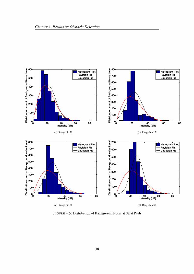
At Pandan reservoir, the background noise was found to be better described by
a Gaussian distribution. Fig. 4.4 shows the distribution of the background noise
for different range bins and the corresponding Gaussian fit. A physical explana-
tion for the background noise being a Gaussian distribution is provided by the
central limit theorem (CLT), which states that the sum of many independent and
identically distributed random variables tends to behave like a Gaussian random
variable [24]. At Pandan reservoir, the bottom is fairly smooth and acts as a
pretty steady reflector which give enough independent scatters and hence the
combined backscatter can be expected to be a Gaussian distribution.
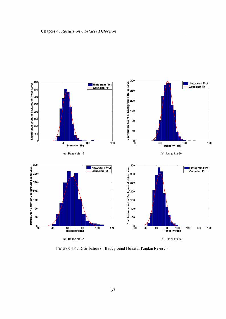
At the sea in Selat Pauh, the background noise did not particularly match
any of the existing distribution for background noise models in literature like the
Gaussian or Rayleigh distribution. A Rayleigh distribution is the amplitude of a
Circularly Symmetric Complex Gaussian distribution. It can be interpreted as a
distribution resulting from the combination of a number of independent scatters
along two perpendicular channels [25, p. 89].
Fig. 4.5 shows the distribution of the background noise for different range
bins and the corresponding Rayleigh and Gaussian fit. It can be seen clearly that
both the Rayleigh and Gaussian fit is not in accordance with the background
noise data obtained at the sea. At the sea in Selat Pauh, the seafloor is more
uneven than at Pandan. This means that the seafloor will not act as a steady re-
flector and one can expect constructive or destructive interference in the signals
received from the reflections off the sea floor. Hence, the individual backscatters
are no longer independent from one another which explains why the background
noise is neither a Gaussian nor a Rayleigh distribution.
36
Chapter 4. Results on Obstacle Detection
0 50 100 1500
50
100
150
200
250
300
350
400
Intensity (dB)
Dis
trib
uti
on
co
un
t o
f B
ac
kg
rou
nd
No
ise
Le
ve
l
Histogram Plot
Gaussian Fit
(a) Range bin 15
0 50 100 1500
50
100
150
200
250
300
Intensity (dB)
Dis
trib
uti
on
co
un
t o
f B
ac
kg
rou
nd
No
ise
Le
ve
l
Histogram Plot
Gaussian Fit
(b) Range bin 20
20 40 60 80 100 1200
50
100
150
200
250
300
350
Intensity (dB)
Dis
trib
uti
on
co
un
t o
f B
ac
kg
rou
nd
No
ise
Le
ve
l
Histogram Plot
Gaussian Fit
(c) Range bin 25
20 40 60 80 100 120 140 1600
50
100
150
200
250
300
350
Intensity (dB)
Dis
trib
uti
on
co
un
t o
f B
ackg
rou
nd
No
ise L
evel
Histogram Plot
Gaussian Fit
(d) Range bin 28
FIGURE 4.4: Distribution of Background Noise at Pandan Reservoir
37
Chapter 4. Results on Obstacle Detection
0 20 40 60 800
100
200
300
400
500
600
Intensity (dB)
Dis
trib
uti
on
co
un
t o
f B
ac
kg
rou
nd
No
ise
Le
ve
l
Histogram Plot
Rayleigh Fit
Gaussian Fit
(a) Range bin 20
0 20 40 60 800
100
200
300
400
500
600
700
800
Intensity (dB)
Dis
trib
uti
on
co
un
t o
f B
ac
kg
rou
nd
No
ise
Le
ve
l
Histogram Plot
Rayleigh Fit
Gaussian Fit
(b) Range bin 25
0 20 40 60 800
100
200
300
400
500
600
700
800
Intensity (dB)
Dis
trib
uti
on
co
un
t o
f B
ac
kg
rou
nd
No
ise
Le
ve
l
Histogram Plot
Rayleigh Fit
Gaussian Fit
(c) Range bin 30
0 20 40 60 800
100
200
300
400
500
600
700
Intensity (dB)
Dis
trib
uti
on
co
un
t o
f B
ac
kg
rou
nd
No
ise
Le
ve
l
Histogram Plot
Rayleigh Fit
Gaussian Fit
(d) Range bin 35
FIGURE 4.5: Distribution of Background Noise at Selat Pauh
38
Chapter 4. Results on Obstacle Detection
4.3 ROC curves, operating pk and tk
FLS scans from the missions at Pandan reservoir and at Selat Pauh as shown
in Fig. 4.3 were analyzed. After marking the obstacles in the map (Fig. 4.3),
we calculated the values of A,B,C and D as per Table 3.1 for different threshold
values, tk, on the measurement, zk,θ . Following this, pk and fk were obtained
as per Eq. 3.1 and Eq. 3.2 respectively. As mentioned in Section 3.1, the plot
of pk vs fk (parametrized by tk) is the receiver operating characteristic (ROC)
curve. This ROC curve varies with signal-to-noise ratio (SNR) and environmen-
tal characteristics.
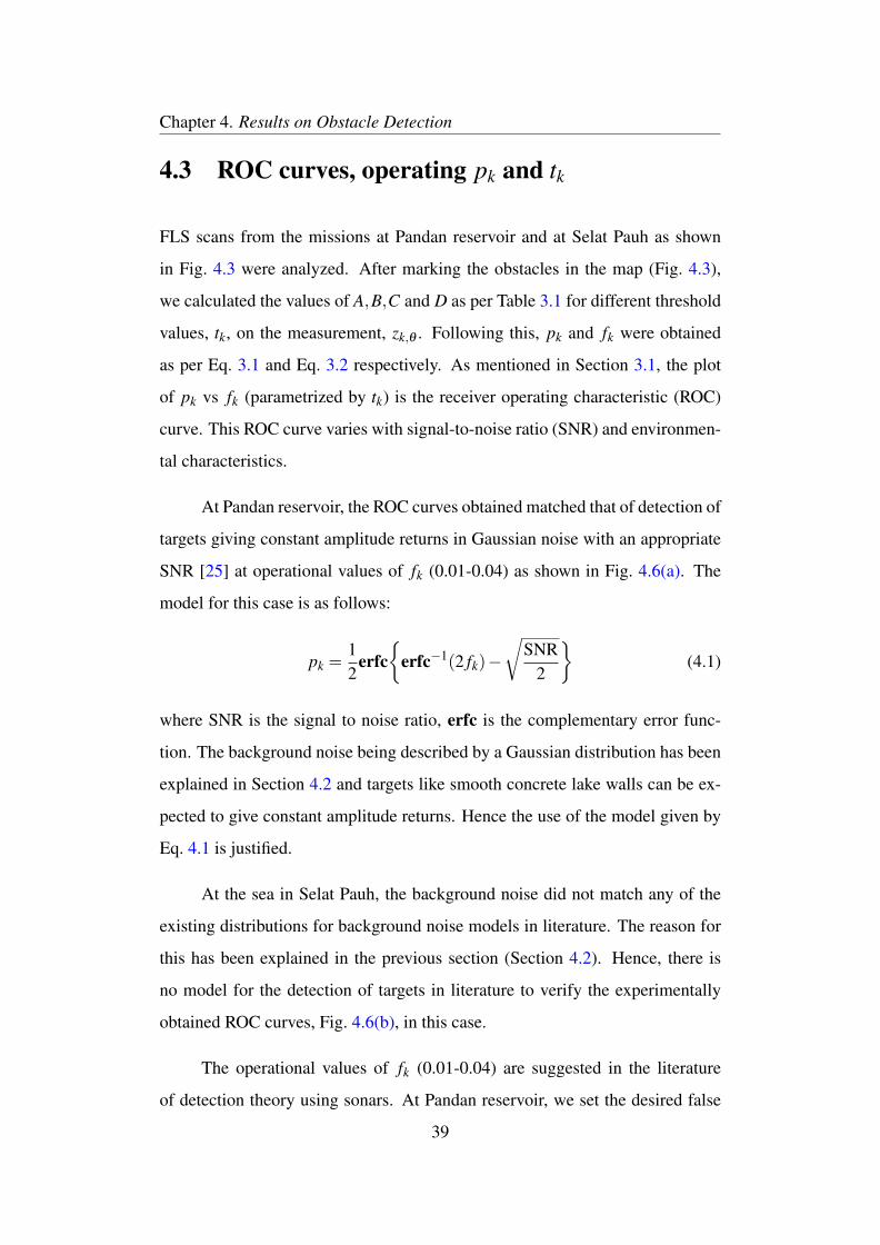
At Pandan reservoir, the ROC curves obtained matched that of detection of
targets giving constant amplitude returns in Gaussian noise with an appropriate
SNR [25] at operational values of fk (0.01-0.04) as shown in Fig. 4.6(a). The
model for this case is as follows:
pk =12
erfc{
erfc−1(2 fk)−√
SNR2
}(4.1)
where SNR is the signal to noise ratio, erfc is the complementary error func-
tion. The background noise being described by a Gaussian distribution has been
explained in Section 4.2 and targets like smooth concrete lake walls can be ex-
pected to give constant amplitude returns. Hence the use of the model given by
Eq. 4.1 is justified.
At the sea in Selat Pauh, the background noise did not match any of the
existing distributions for background noise models in literature. The reason for
this has been explained in the previous section (Section 4.2). Hence, there is
no model for the detection of targets in literature to verify the experimentally
obtained ROC curves, Fig. 4.6(b), in this case.
The operational values of fk (0.01-0.04) are suggested in the literature
of detection theory using sonars. At Pandan reservoir, we set the desired false
39
Chapter 4. Results on Obstacle Detection
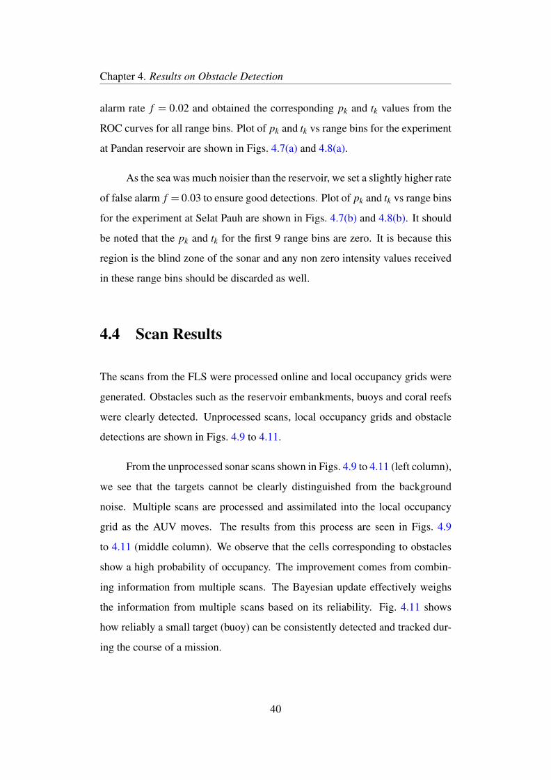
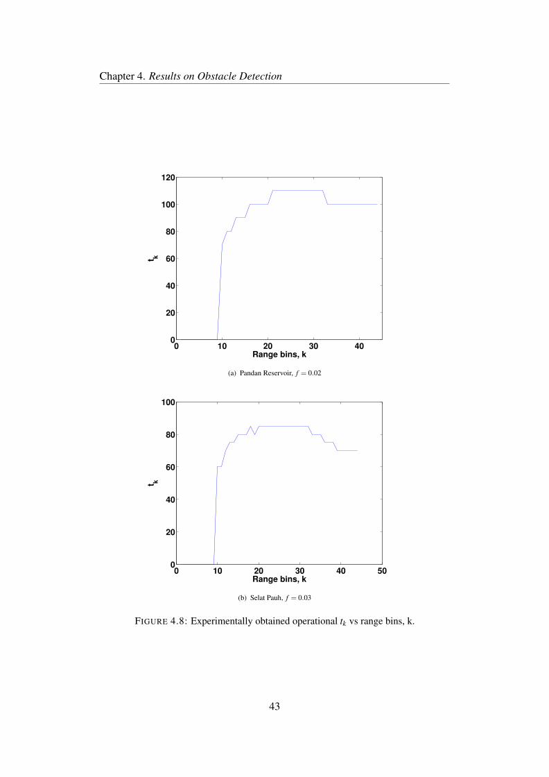
alarm rate f = 0.02 and obtained the corresponding pk and tk values from the
ROC curves for all range bins. Plot of pk and tk vs range bins for the experiment
at Pandan reservoir are shown in Figs. 4.7(a) and 4.8(a).
As the sea was much noisier than the reservoir, we set a slightly higher rate
of false alarm f = 0.03 to ensure good detections. Plot of pk and tk vs range bins
for the experiment at Selat Pauh are shown in Figs. 4.7(b) and 4.8(b). It should
be noted that the pk and tk for the first 9 range bins are zero. It is because this
region is the blind zone of the sonar and any non zero intensity values received
in these range bins should be discarded as well.
4.4 Scan Results
The scans from the FLS were processed online and local occupancy grids were
generated. Obstacles such as the reservoir embankments, buoys and coral reefs
were clearly detected. Unprocessed scans, local occupancy grids and obstacle
detections are shown in Figs. 4.9 to 4.11.
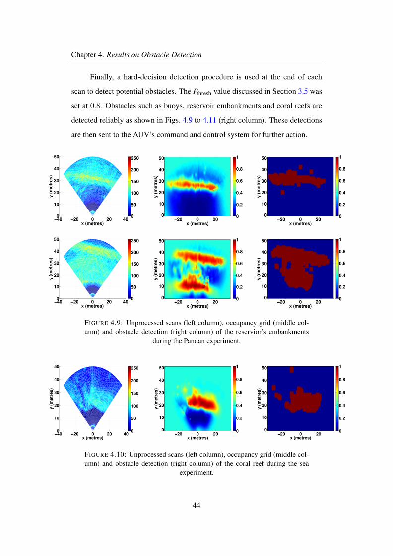
From the unprocessed sonar scans shown in Figs. 4.9 to 4.11 (left column),
we see that the targets cannot be clearly distinguished from the background
noise. Multiple scans are processed and assimilated into the local occupancy
grid as the AUV moves. The results from this process are seen in Figs. 4.9
to 4.11 (middle column). We observe that the cells corresponding to obstacles
show a high probability of occupancy. The improvement comes from combin-
ing information from multiple scans. The Bayesian update effectively weighs
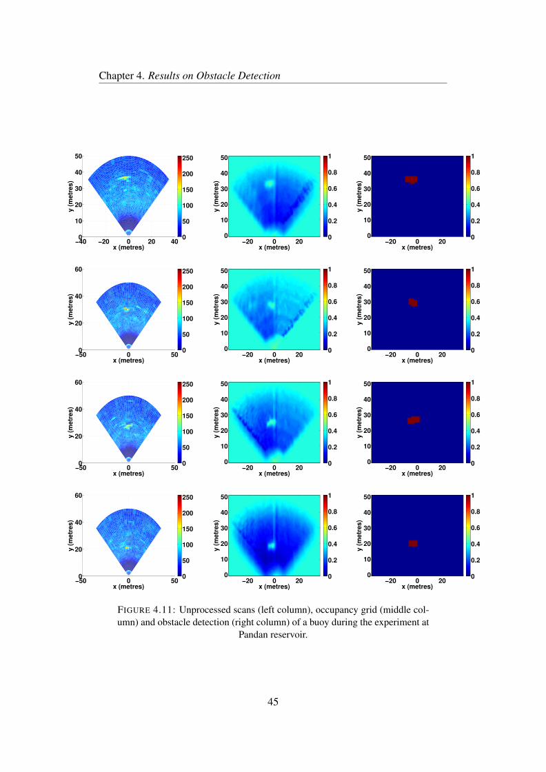
the information from multiple scans based on its reliability. Fig. 4.11 shows
how reliably a small target (buoy) can be consistently detected and tracked dur-
ing the course of a mission.
40
Chapter 4. Results on Obstacle Detection
0 0.01 0.02 0.03 0.04 0.050
0.1
0.2
0.3
0.4
0.5
0.6
0.7
0.8
fk
pk
Range bin, k = 25
Theoretical Model, SNR = 7.0
Range bin, k = 33
Theoretical Model, SNR = 6.0
Range bin, k = 40
Theoretical Model, SNR = 5.0
(a) ROC plot at Pandan Reservoir and the corresponding theoretical curves
0 0.01 0.02 0.03 0.040
0.1
0.2
0.3
0.4
0.5
0.6
0.7
0.8
0.9
1
fk
pk
Range bin, k = 35
Range bin, k = 30
Range bin, k = 25
Range bin, k = 20
(b) ROC plot at Selat Pauh
FIGURE 4.6: Experimentally obtained ROC plots.
41
Chapter 4. Results on Obstacle Detection
0 10 20 30 400
0.1
0.2
0.3
0.4
0.5
0.6
0.7
Range bins, k
pk
(a) Pandan Reservoir, f = 0.02
0 10 20 30 400
0.1
0.2
0.3
0.4
0.5
0.6
0.7
0.8
Range bins, k
pk
(b) Selat Pauh, f = 0.03
FIGURE 4.7: Experimentally obtained operational pk vs range bins, k.
42
Chapter 4. Results on Obstacle Detection
0 10 20 30 400
20
40
60
80
100
120
Range bins, k
t k
(a) Pandan Reservoir, f = 0.02
0 10 20 30 40 500
20
40
60
80
100
Range bins, k
t k
(b) Selat Pauh, f = 0.03
FIGURE 4.8: Experimentally obtained operational tk vs range bins, k.
43
Chapter 4. Results on Obstacle Detection
Finally, a hard-decision detection procedure is used at the end of each
scan to detect potential obstacles. The Pthresh value discussed in Section 3.5 was
set at 0.8. Obstacles such as buoys, reservoir embankments and coral reefs are
detected reliably as shown in Figs. 4.9 to 4.11 (right column). These detections
are then sent to the AUV’s command and control system for further action.
−40 −20 0 20 400
10
20
30
40
50
x (metres)
y (
metr
es)
0
50
100
150
200
250
x (metres)
y (
metr
es)
−20 0 200
10
20
30
40
50
0
0.2
0.4
0.6
0.8
1
x (metres)
y (
metr
es)
−20 0 200
10
20
30
40
50
0
0.2
0.4
0.6
0.8
1
−40 −20 0 20 400
10
20
30
40
50
x (metres)
y (
metr
es)
0
50
100
150
200
250
x (metres)
y (
metr
es)
−20 0 200
10
20
30
40
50
0
0.2
0.4
0.6
0.8
1
x (metres)
y (
metr
es)
−20 0 200
10
20
30
40
50
0
0.2
0.4
0.6
0.8
1
FIGURE 4.9: Unprocessed scans (left column), occupancy grid (middle col-umn) and obstacle detection (right column) of the reservior’s embankments
during the Pandan experiment.
−40 −20 0 20 400
10
20
30
40
50
x (metres)
y (
me
tre
s)
0
50
100
150
200
250
x (metres)
y (
metr
es)
−20 0 200
10
20
30
40
50
0
0.2
0.4
0.6
0.8
1
x (metres)
y (
metr
es)
−20 0 200
10
20
30
40
50
0
0.2
0.4
0.6
0.8
1
FIGURE 4.10: Unprocessed scans (left column), occupancy grid (middle col-umn) and obstacle detection (right column) of the coral reef during the sea
experiment.
44
Chapter 4. Results on Obstacle Detection
−40 −20 0 20 400
10
20
30
40
50
x (metres)
y (
metr
es)
0
50
100
150
200
250
x (metres)
y (
metr
es)
−20 0 200
10
20
30
40
50
0
0.2
0.4
0.6
0.8
1
x (metres)
y (
metr
es)
−20 0 200
10
20
30
40
50
0
0.2
0.4
0.6
0.8
1
−50 0 500
20
40
60
x (metres)
y (
metr
es)
0
50
100
150
200
250
x (metres)
y (
metr
es)
−20 0 200
10
20
30
40
50
0
0.2
0.4
0.6
0.8
1
x (metres)y (
metr
es)
−20 0 200
10
20
30
40
50
0
0.2
0.4
0.6
0.8
1
−50 0 500
20
40
60
x (metres)
y (
metr
es)
0
50
100
150
200
250
x (metres)
y (
metr
es)
−20 0 200
10
20
30
40
50
0
0.2
0.4
0.6
0.8
1
x (metres)
y (
metr
es)
−20 0 200
10
20
30
40
50
0
0.2
0.4
0.6
0.8
1
−50 0 500
20
40
60
x (metres)
y (
metr
es)
0
50
100
150
200
250
x (metres)
y (
metr
es)
−20 0 200
10
20
30
40
50
0
0.2
0.4
0.6
0.8
1
x (metres)
y (
metr
es)
−20 0 200
10
20
30
40
50
0
0.2
0.4
0.6
0.8
1
FIGURE 4.11: Unprocessed scans (left column), occupancy grid (middle col-umn) and obstacle detection (right column) of a buoy during the experiment at
Pandan reservoir.
45
Chapter 4. Results on Obstacle Detection
4.5 Summary
Experiments were conducted at both lake and sea environments. While the back-
ground noise at Pandan reservoir was found to model a Gaussian distribution,
at the sea it was better described by a Rayleigh distribution. ROC curves were
obtained experimentally and were verified with an existing mathematical model
for the curves obtained from the experiment at Pandan Reservoir. An operational
false alarm rate, f , was set following which pk and tk were obtained from the
ROC curves. Finally, local occupancy grids were generated using a Bayesian ap-
proach after processing the raw scans and obstacles were consistently detected.
The detected obstacles would be sent to the command and control (C2) system
of the AUV to carry out evasive maneuvers if necessary.
46
Chapter 5
Command and Control
Architechture for STARFISH AUV
This chapter presents the command and control architecture used in the STARFISH
AUVs [26] and how the obstacle avoidance component was incorporated into
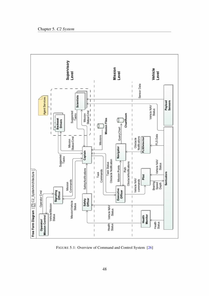
the C2 system. An overview of the architectural design is illustrated in Fig. 5.1.
This is followed by a brief description of the C2 architecture and its important
components. Finally, the obstacle avoidance component and its integration into
the C2 system is discussed.
5.1 The C2 Architecture
Command and control system perform tasks ranging from planning, coordinat-
ing, directing and controlling varies activities in an AUV. It receives the pro-
cessed data from the sensors as inputs and then outputs the control commands
to the actuators to generate the desired behavior to achieve the mission objective
while keeping the AUV safe throughout the mission execution.
47
Chapter 5. C2 System
FLSDetector
FIGURE 5.1: Overview of Command and Control System [26]
48
Chapter 5. C2 System
The C2 architecture used in the STARFISH AUV is based on a hybrid
hierarchical control architecture as shown in Fig. 5.1. It adopts a deliberative-
reactive architecture that consists of having core components, also known as
agents, arranged in three different levels of control hierarchy. The three levels
are as follows: Supervisory level, Mission level and Vehicle level.
The Supervisory level is in charge of commanding and monitoring the
high level mission and vehicle status while ensuring the vehicle’s safety through-
out the mission. An external communication component (Signaling Officer) has
been built to provide communication link with the operator or with another AUV.
It also falls under the Supervisory level. The Mission level is responsible for
mission path planning and re-planning in the event of a likely collision. Finally,
the Vehicle level carries out the mission tasks and performs obstacle avoidance
by utilizing different Sentuators (sensors and actuators) to generate the desired
behavior.
Each agent implements its own algorithm depending on the task it is as-
signed. All agents are self contained within a uniform software platform to
facilitate inter-agent communication. Communication occurs through message
passing. The vehicle’s tasks are complete with the help of interaction between
different agents. This type of agent-based approach gives flexibility to the ar-
chitecture with respect to the implementation aspect. It is because, rather than
modifying existing software components to add new features, agents can be built
instead and loaded whenever it needs to be used.
Following are the descriptions of the functions of important agents in the
C2 system:
1. Captain: All high level supervisory tasks are carried out by the Captain.
It is responsible for starting and coordinating the execution of missions. It
also receives safety updates of the AUV from the Safety Officer continu-
ously. During the execution of a mission, if anything abnormal is reported
49
Chapter 5. C2 System
by the Safety officer, the mission is aborted immediately. It receives the
mission planning request sent by the Operator via the Signaling Officer
agent. It then broadcasts the request to all available Backseat Drivers to
find the most suitable one which can carry out that specific task.
2. Executive Officer: It receives mission tasks in the form of mission points
from the Captain. These missions points are then sent to the Navigator
for path planning. The Navigator then returns a set of waypoints to reach
a particular mission point. Hence, each mission point is associated with
a set of waypoints. Finally, the waypoints are sent to the Pilot to be ex-
ecuted. If there is any change in the waypoints of a mission point being
executed due to the presence of an obstacle, the Captain is notified of the
execution of an avoidance maneuver.
3. Navigator: It receives the mission point from the Executive Officer and
plans waypoints to reach the mission point and sends it back to the Ex-
ecutive Officer. Fig. 5.2 shows the waypoints and the mission points for
a mission planned at Pandan reservoir. Mission points are user defined
and are stored in a Mission File while the waypoints are generated by the
Navigator of the AUV.
It also receives a local map of the obstacles present in the vicinity of the
AUV at regular intervals from the FLSDetector. It then checks if there is
any possible collision with the obstacles and re-plans a new set of way-
points. More details are discussed in Section 5.2.
4. Pilot: It receives the waypoints to be executed from the Executive Officer.
Each waypoint is executed in a systematic manner by defining set-points
for the following vehicle parameters: bearing, speed, depth and altitude.
Once, all the waypoints associated with a mission point is executed, the
mission point considered to be reached and the next set of waypoints are
executed.
50
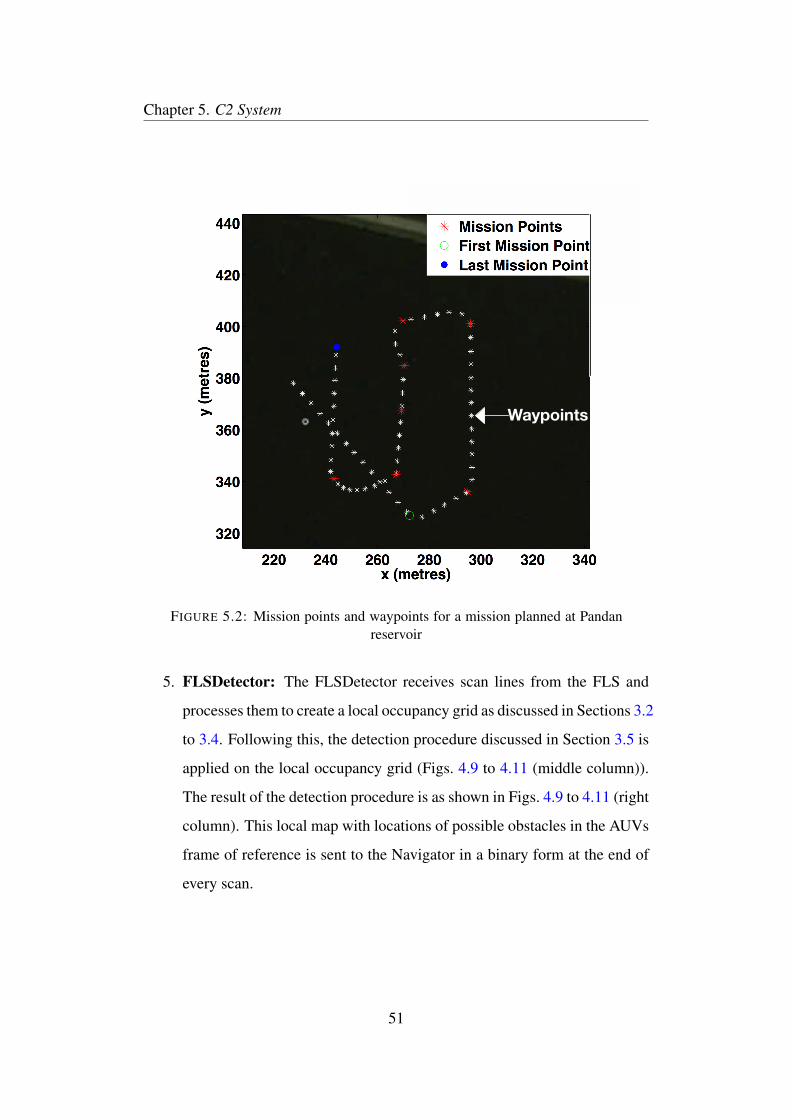
Chapter 5. C2 System
Waypoints
FIGURE 5.2: Mission points and waypoints for a mission planned at Pandanreservoir
5. FLSDetector: The FLSDetector receives scan lines from the FLS and
processes them to create a local occupancy grid as discussed in Sections 3.2
to 3.4. Following this, the detection procedure discussed in Section 3.5 is
applied on the local occupancy grid (Figs. 4.9 to 4.11 (middle column)).
The result of the detection procedure is as shown in Figs. 4.9 to 4.11 (right
column). This local map with locations of possible obstacles in the AUVs
frame of reference is sent to the Navigator in a binary form at the end of
every scan.
51
Chapter 5. C2 System
5.2 Obstacle Avoidance
A local avoidance approach to obstacle avoidance has been adopted in our work.
This is because the AUV executes an avoidance behavior as and when it sees an
obstacle which poses a threat of collision.
From Fig. 5.1, it can be seen that the principle components involved in
obstacle avoidance are the FLSDetector and the Navigator. Their detailed func-
tionalities are discussed in Sections 5.2.1 and 5.2.2. Fig. 5.3 shows a flow chart
describing the flow of control during the obstacle avoidance stage.
5.2.1 FLSDetector
The FLSDetector directly communicates with the FLS and receives scan lines
continuously from the sonar. It processes these scan lines as per the methods
discussed in Sections 3.2 to 3.4 to generate a local occupancy grid. After this,
an obstacle detection procedure (Section 3.5) is used at the end of a complete
scan to detect likely obstacles in the vicinity of the AUV. This procedure creates
a detection map in the AUVs frame of reference. The detection map is then sent
to the Navigator of the AUV for further actions.
5.2.2 Navigator
Once the Navigator receives a detection map from the FLSDetector, it creates a
new map with the obstacles inflated so as to provide a clearance radius during
obstacle avoidance maneuvers. The obstacles are inflated such that if the size of
each cell in the detection map is l× l, the size of each cell in the new map created
by the Navigator would be o× o such that o > l. Fig. 5.4 shows the detection
map sent by the FLSDetector and new map generated by the Navigator.
52
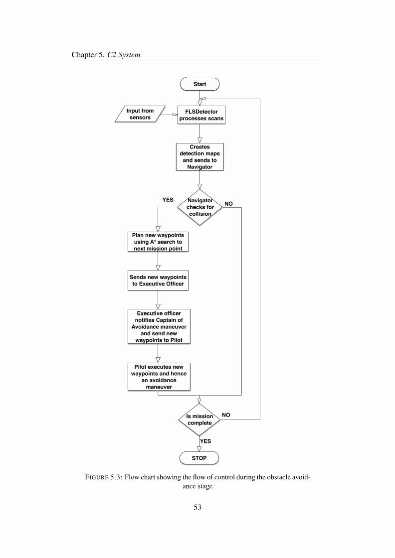
Chapter 5. C2 System
Start
Input from
sensors FLSDetector
processes scans
Plan new waypoints
using A* search to
next mission point
Navigator
checks for
collision
YESNO
Is mission
complete
YES
STOP
NO
Creates
detection maps
and sends to
Navigator
Sends new waypoints
to Executive Officer
Executive officer
notifies Captain of
Avoidance maneuver
and send new
waypoints to Pilot
Pilot executes new
waypoints and hence
an avoidance
maneuver
FIGURE 5.3: Flow chart showing the flow of control during the obstacle avoid-ance stage
53
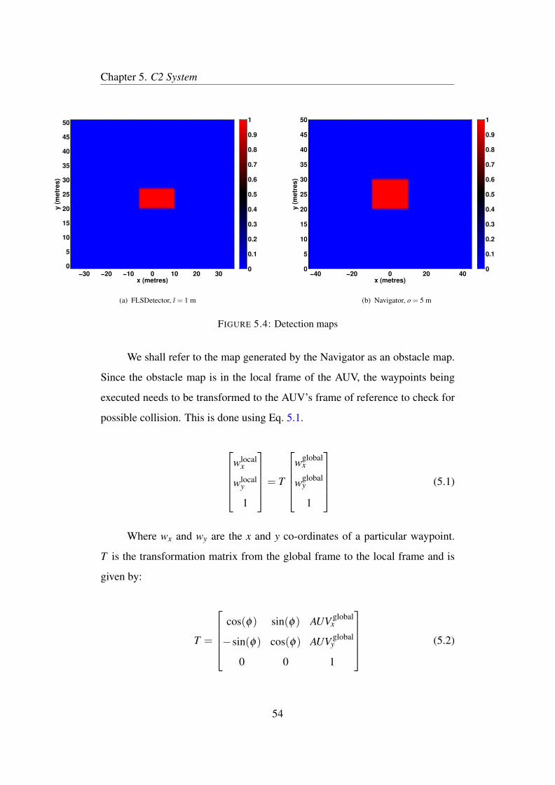
Chapter 5. C2 System
x (metres)
y (
metr
es)
−30 −20 −10 0 10 20 300
5
10
15
20
25
30
35
40
45
50
0
0.1
0.2
0.3
0.4
0.5
0.6
0.7
0.8
0.9
1
(a) FLSDetector, l = 1 m
x (metres)
y (
metr
es)
−40 −20 0 20 400
5
10
15
20
25
30
35
40
45
50
0
0.1
0.2
0.3
0.4
0.5
0.6
0.7
0.8
0.9
1
(b) Navigator, o = 5 m
FIGURE 5.4: Detection maps
We shall refer to the map generated by the Navigator as an obstacle map.
Since the obstacle map is in the local frame of the AUV, the waypoints being
executed needs to be transformed to the AUV’s frame of reference to check for
possible collision. This is done using Eq. 5.1.
wlocal
x
wlocaly
1
= T
wglobal
x
wglobaly
1
(5.1)
Where wx and wy are the x and y co-ordinates of a particular waypoint.
T is the transformation matrix from the global frame to the local frame and is
given by:
T =
cos(φ) sin(φ) AUV global
x
−sin(φ) cos(φ) AUV globaly
0 0 1
(5.2)
54
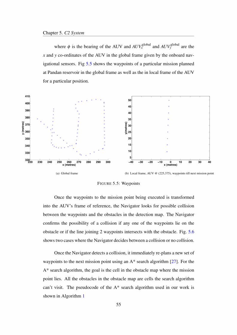
Chapter 5. C2 System
where φ is the bearing of the AUV and AUV globalx and AUV global
y are the
x and y co-ordinates of the AUV in the global frame given by the onboard nav-
igational sensors. Fig 5.5 shows the waypoints of a particular mission planned
at Pandan reservoir in the global frame as well as the in local frame of the AUV
for a particular position.
220 230 240 250 260 270 280 290 300320
330
340
350
360
370
380
390
400
410
x (metres)
y (
metr
es)
(a) Global frame
−40 −30 −20 −10 0 10 20 30 40
5
10
15
20
25
30
35
40
45
50
x (metres)
y(m
etr
es)
(b) Local frame, AUV @ (225,375), waypoints till next mission point
FIGURE 5.5: Waypoints
Once the waypoints to the mission point being executed is transformed
into the AUV’s frame of reference, the Navigator looks for possible collision
between the waypoints and the obstacles in the detection map. The Navigator
confirms the possibility of a collision if any one of the waypoints lie on the
obstacle or if the line joining 2 waypoints intersects with the obstacle. Fig. 5.6
shows two cases where the Navigator decides between a collision or no collision.
Once the Navigator detects a collision, it immediately re-plans a new set of
waypoints to the next mission point using an A* search algorithm [27]. For the
A* search algorithm, the goal is the cell in the obstacle map where the mission
point lies. All the obstacles in the obstacle map are cells the search algorithm
can’t visit. The pseudocode of the A* search algorithm used in our work is
shown in Algorithm 1
55
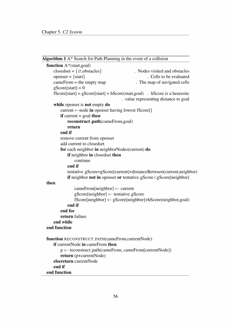
Chapter 5. C2 System
Algorithm 1 A* Search for Path Planning in the event of a collisionfunction A*(start,goal)
closedset = {∅,obstacles} . Nodes visited and obstaclesopenset = {start} . Cells to be evaluatedcameFrom = the empty map . The map of navigated cellsgScore[start] = 0fScore[start] = gScore[start] + hScore(start,goal) . hScore is a heurestic
. value representing distance to goalwhile openset is not empty do
current←node in openset having lowest fScore[]if current = goal then
reconstruct path(cameFrom,goal)return
end ifremove current from opensetadd current to closedsetfor each neighbor in neighborNodes(current) do
if neighbor in closedset thencontinue
end iftentative gScore=gScore[current]+distanceBetween(current,neighbor)if neighbor not in openset or tentative gScore<gScore[neighbor]
thencameFrom[neighbor]← currentgScore[neighbor]← tentative gScorefScore[neighbor]← gScore[neighbor]+hScore(neighbor,goal)
end ifend forreturn failure
end whileend function
function RECONSTRUCT PATH(cameFrom,currentNode)if currentNode in cameFrom then
p← reconstruct path(cameFrom, cameFrom[currentNode])return (p+currentNode)
elsereturn currentNodeend if
end function
56
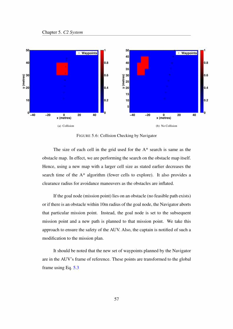
Chapter 5. C2 System
x (metres)
y (
me
tres
)
−40 −20 0 20 400
10
20
30
40
50
0
0.2
0.4
0.6
0.8
1Waypoints
(a) Collision
x (metres)
y (
me
tres
)
−40 −20 0 20 40
5
10
15
20
25
30
35
40
45
50
0
0.2
0.4
0.6
0.8
1Waypoints
(b) No Collision
FIGURE 5.6: Collision Checking by Navigator
The size of each cell in the grid used for the A* search is same as the
obstacle map. In effect, we are performing the search on the obstacle map itself.
Hence, using a new map with a larger cell size as stated earlier decreases the
search time of the A* algorithm (fewer cells to explore). It also provides a
clearance radius for avoidance maneuvers as the obstacles are inflated.
If the goal node (mission point) lies on an obstacle (no feasible path exists)
or if there is an obstacle within 10m radius of the goal node, the Navigator aborts
that particular mission point. Instead, the goal node is set to the subsequent
mission point and a new path is planned to that mission point. We take this
approach to ensure the safety of the AUV. Also, the captain is notified of such a
modification to the mission plan.
It should be noted that the new set of waypoints planned by the Navigator
are in the AUV’s frame of reference. These points are transformed to the global
frame using Eq. 5.3
57
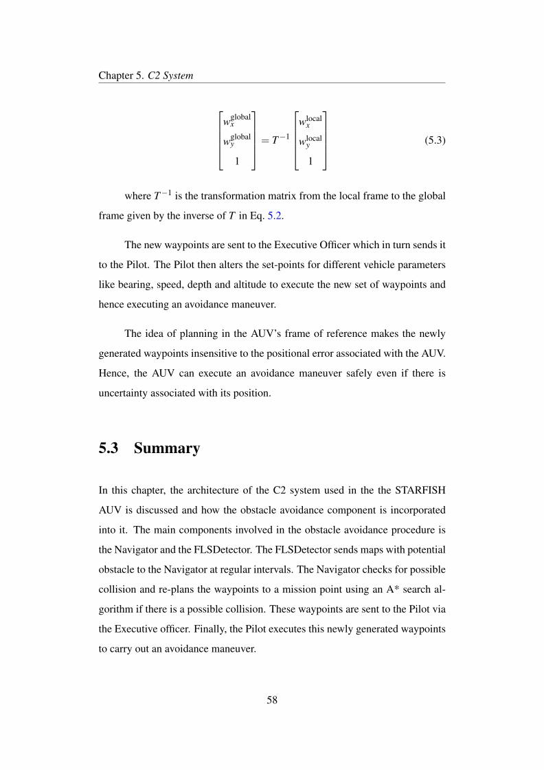
Chapter 5. C2 System
wglobal
x
wglobaly
1
= T−1
wlocal
x
wlocaly
1
(5.3)
where T−1 is the transformation matrix from the local frame to the global
frame given by the inverse of T in Eq. 5.2.
The new waypoints are sent to the Executive Officer which in turn sends it
to the Pilot. The Pilot then alters the set-points for different vehicle parameters
like bearing, speed, depth and altitude to execute the new set of waypoints and
hence executing an avoidance maneuver.
The idea of planning in the AUV’s frame of reference makes the newly
generated waypoints insensitive to the positional error associated with the AUV.
Hence, the AUV can execute an avoidance maneuver safely even if there is
uncertainty associated with its position.
5.3 Summary
In this chapter, the architecture of the C2 system used in the the STARFISH
AUV is discussed and how the obstacle avoidance component is incorporated
into it. The main components involved in the obstacle avoidance procedure is
the Navigator and the FLSDetector. The FLSDetector sends maps with potential
obstacle to the Navigator at regular intervals. The Navigator checks for possible
collision and re-plans the waypoints to a mission point using an A* search al-
gorithm if there is a possible collision. These waypoints are sent to the Pilot via
the Executive officer. Finally, the Pilot executes this newly generated waypoints
to carry out an avoidance maneuver.
58
Chapter 6
Results on Obstacle Avoidance
In this chapter, we present results of obstacle avoidance using the C2 system
described in Chapter 5. Results from both simulation studies and experiments
from field trials are discussed in Sections 6.1 and 6.2.
6.1 Simulation Studies
The C2 system described in Chapter 5 was implemented using the fjage agent
framework [28] by Tan et al [26] for the STARFISH project. The simulator en-
vironment has also been implemented using a separate fjage agent container. It
uses a simplified dynamic model for the AUV. The AUV in the simulator ac-
cepts actuator commands and produces simulated sensor data, as if they were
generated by the physical AUV. Since the C2 system uses an agent-based design
and inter agent communication takes place through a message passing mecha-
nism, the C2 system can be decoupled from the physical vehicle’s sensors and
actuators. This allows the resultant C2 system to be tested through simulation.
Once tested, the same C2 system can be loaded into a physical AUV for field
59
Chapter 6. Results on Obstacle Avoidance
experiments without any modification. This Simulation-In-The-Loop method-
ology expedites the design and development of new C2 capabilities and shorten
mission turn-around time [29].
In the simulation, we demonstrate the capability of an AUV in a simulator
environment running the C2 system described in Chapter 5 to perform an ob-
stacle avoidance maneuver. We refer to Chapter 5 for detailed algorithms. The
setup is such that missions are planned by the Operator and requested to be exe-
cuted by the CAPTAIN of the simulator AUV. Once the mission has started and
after some amount of time has lapsed, the FLSDetector sends a detection map
(generated by the user) to the Navigator. The Navigator of the AUV analyzes
the detection map and decides if there is a possibility of a collision and re-plans
the waypoints if necessary.
We verify the proper functioning of the agents involved in the obstacle
avoidance procedure by testing the agents’ behaviour for a single detection map
in the simulation. It can be seen that the simulation setup can easily be decou-
pled from the physical components of the AUV.
6.1.1 Results
Fig. 6.1 shows two missions planned by the Operator for the simulator AUV
to execute. Each mission had 3 mission points to be executed. In Fig. 6.1,
the boundary in the map (geofence) is the admissible operational region for the
AUV. If the AUV were to go out of the geofence during a mission, the Safety
Officer would immediately abort the mission.
The FLSDetector sent two different detections maps, one for each mission,
to the Navigator as shown in Fig. 6.2. The maps were sent exactly 10 seconds
after the mission had started.
60
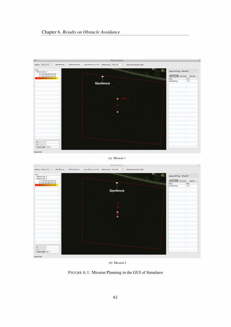
Chapter 6. Results on Obstacle Avoidance
Geofence
(a) Mission 1
Geofence
(b) Mission 2
FIGURE 6.1: Mission Planning in the GUI of Simulator
61
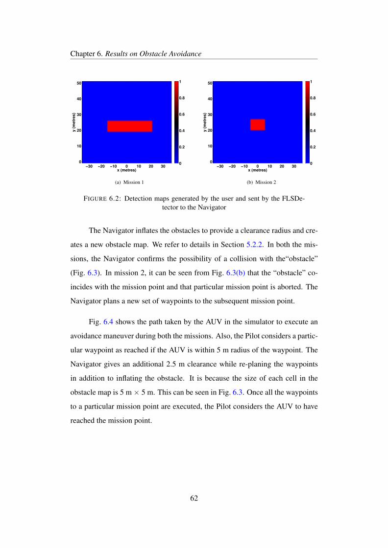
Chapter 6. Results on Obstacle Avoidance
x (metres)
y (
metr
es)
−30 −20 −10 0 10 20 300
10
20
30
40
50
0
0.2
0.4
0.6
0.8
1
(a) Mission 1
x (metres)
y (
metr
es)
−30 −20 −10 0 10 20 300
10
20
30
40
50
0
0.2
0.4
0.6
0.8
1
(b) Mission 2
FIGURE 6.2: Detection maps generated by the user and sent by the FLSDe-tector to the Navigator
The Navigator inflates the obstacles to provide a clearance radius and cre-
ates a new obstacle map. We refer to details in Section 5.2.2. In both the mis-
sions, the Navigator confirms the possibility of a collision with the“obstacle”
(Fig. 6.3). In mission 2, it can be seen from Fig. 6.3(b) that the “obstacle” co-
incides with the mission point and that particular mission point is aborted. The
Navigator plans a new set of waypoints to the subsequent mission point.
Fig. 6.4 shows the path taken by the AUV in the simulator to execute an
avoidance maneuver during both the missions. Also, the Pilot considers a partic-
ular waypoint as reached if the AUV is within 5 m radius of the waypoint. The
Navigator gives an additional 2.5 m clearance while re-planing the waypoints
in addition to inflating the obstacle. It is because the size of each cell in the
obstacle map is 5 m× 5 m. This can be seen in Fig. 6.3. Once all the waypoints
to a particular mission point are executed, the Pilot considers the AUV to have
reached the mission point.
62
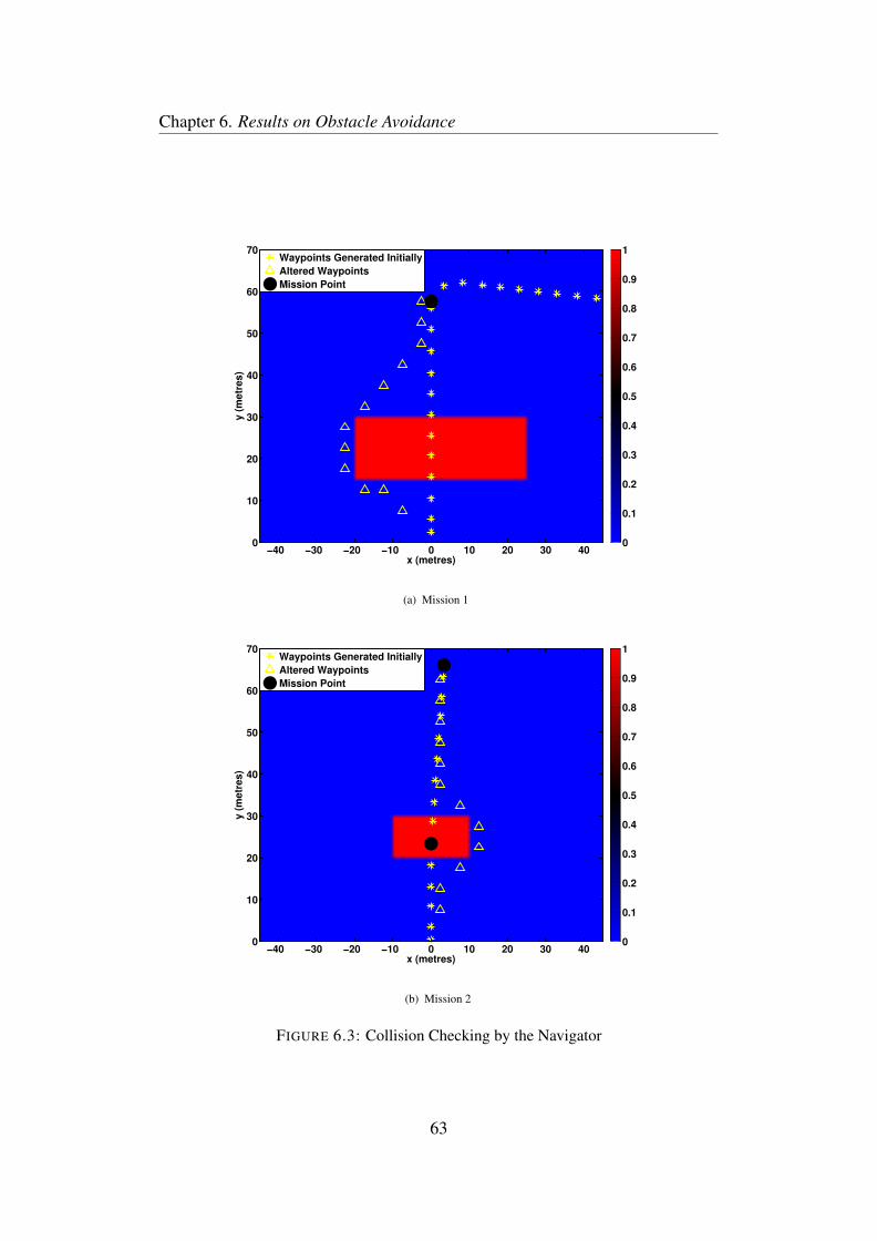
Chapter 6. Results on Obstacle Avoidance
x (metres)
y (
me
tre
s)
−40 −30 −20 −10 0 10 20 30 400
10
20
30
40
50
60
70Waypoints Generated Initially
Altered Waypoints
Mission Point
0
0.1
0.2
0.3
0.4
0.5
0.6
0.7
0.8
0.9
1
(a) Mission 1
x (metres)
y (
me
tre
s)
−40 −30 −20 −10 0 10 20 30 400
10
20
30
40
50
60
70Waypoints Generated Initially
Altered Waypoints
Mission Point
0
0.1
0.2
0.3
0.4
0.5
0.6
0.7
0.8
0.9
1
(b) Mission 2
FIGURE 6.3: Collision Checking by the Navigator
63
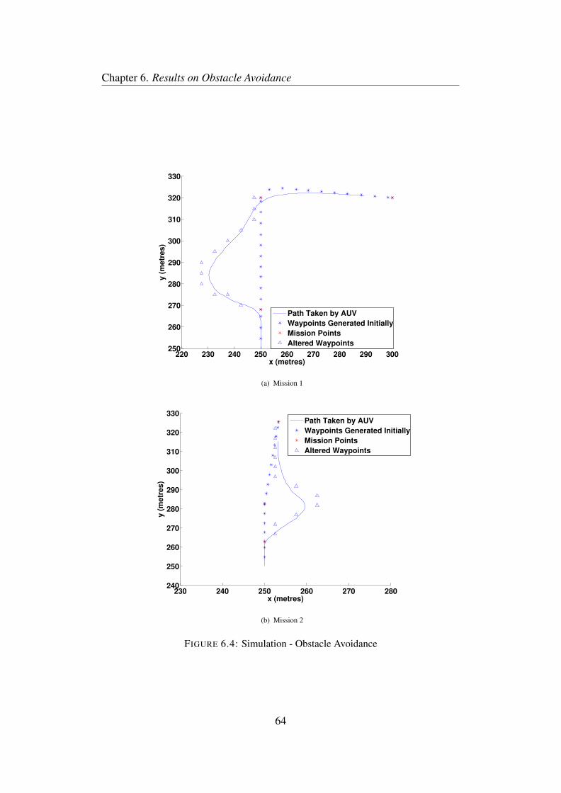
Chapter 6. Results on Obstacle Avoidance
220 230 240 250 260 270 280 290 300250
260
270
280
290
300
310
320
330
x (metres)
y (
metr
es)
Path Taken by AUV
Waypoints Generated Initially
Mission Points
Altered Waypoints
(a) Mission 1
230 240 250 260 270 280240
250
260
270
280
290
300
310
320
330
x (metres)
y (
metr
es)
Path Taken by AUV
Waypoints Generated Initially
Mission Points
Altered Waypoints
(b) Mission 2
FIGURE 6.4: Simulation - Obstacle Avoidance
64
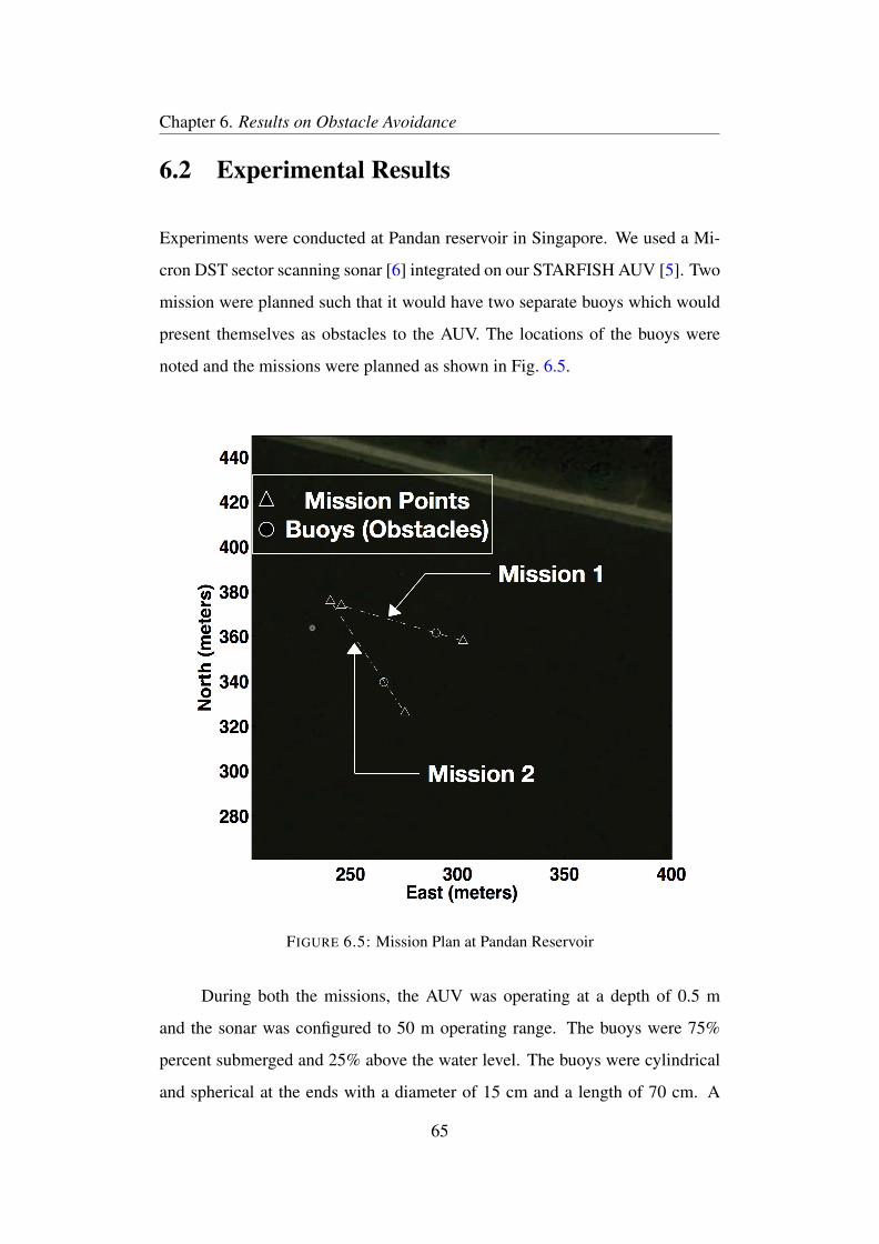
Chapter 6. Results on Obstacle Avoidance
6.2 Experimental Results
Experiments were conducted at Pandan reservoir in Singapore. We used a Mi-
cron DST sector scanning sonar [6] integrated on our STARFISH AUV [5]. Two
mission were planned such that it would have two separate buoys which would
present themselves as obstacles to the AUV. The locations of the buoys were
noted and the missions were planned as shown in Fig. 6.5.
Mission 1
Mission 2
Mission Points
Buoys (Obstacles)
FIGURE 6.5: Mission Plan at Pandan Reservoir
During both the missions, the AUV was operating at a depth of 0.5 m
and the sonar was configured to 50 m operating range. The buoys were 75%
percent submerged and 25% above the water level. The buoys were cylindrical
and spherical at the ends with a diameter of 15 cm and a length of 70 cm. A
65
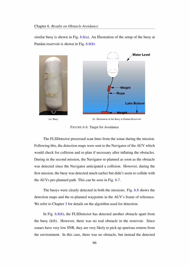
Chapter 6. Results on Obstacle Avoidance
similar buoy is shown in Fig. 6.6(a). An Illustration of the setup of the buoy at
Pandan reservoir is shown in Fig. 6.6(b)
(a) Buoy
Weight
(b) Illustration of the Buoy at Pandan Reservoir
FIGURE 6.6: Target for Avoidance
The FLSDetector processed scan lines from the sonar during the mission.
Following this, the detection maps were sent to the Navigator of the AUV which
would check for collision and re-plan if necessary after inflating the obstacles.
During in the second mission, the Navigator re-planned as soon as the obstacle
was detected since the Navigator anticipated a collision. However, during the
first mission, the buoy was detected much earlier but didn’t seem to collide with
the AUVs pre-planned path. This can be seen in Fig. 6.7.
The buoys were clearly detected in both the missions. Fig. 6.8 shows the
detection maps and the re-planned waypoints in the AUV’s frame of reference.
We refer to Chapter 3 for details on the algorithm used for detection.
In Fig. 6.8(b), the FLSDetector has detected another obstacle apart from
the buoy (left). However, there was no real obstacle in the reservoir. Since
sonars have very low SNR, they are very likely to pick up spurious returns from
the environment. In this case, there was no obstacle, but instead the detected
66
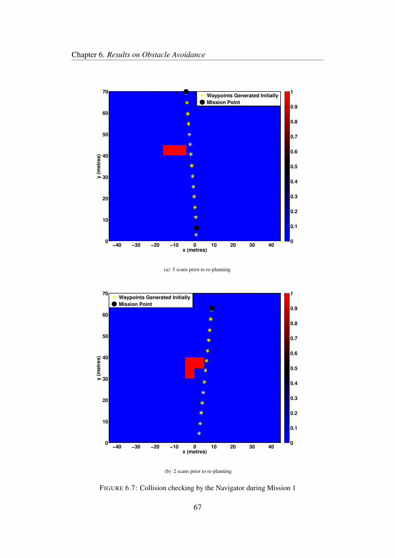
Chapter 6. Results on Obstacle Avoidance
x (metres)
y (
metr
es)
−40 −30 −20 −10 0 10 20 30 400
10
20
30
40
50
60
70Waypoints Generated Initially
Mission Point
0
0.1
0.2
0.3
0.4
0.5
0.6
0.7
0.8
0.9
1
(a) 5 scans prior to re-planning
x (metres)
y (
metr
es)
−40 −30 −20 −10 0 10 20 30 400
10
20
30
40
50
60
70Waypoints Generated Initially
Mission Point
0
0.1
0.2
0.3
0.4
0.5
0.6
0.7
0.8
0.9
1
(b) 2 scans prior to re-planning
FIGURE 6.7: Collision checking by the Navigator during Mission 1
67
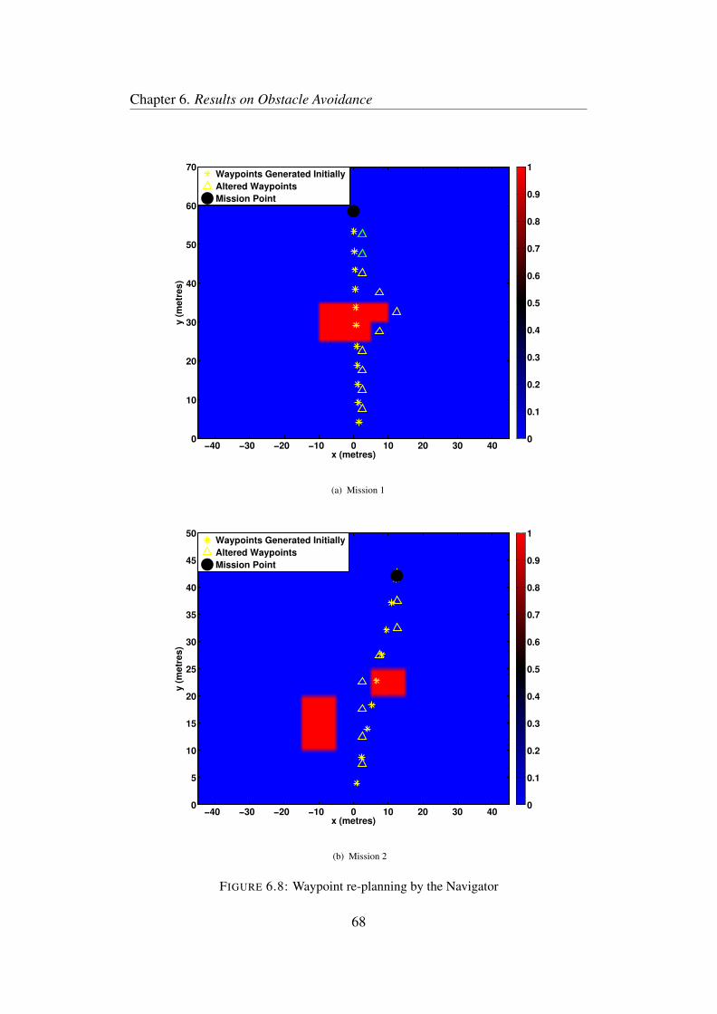
Chapter 6. Results on Obstacle Avoidance
x (metres)
y (
metr
es)
−40 −30 −20 −10 0 10 20 30 400
10
20
30
40
50
60
70Waypoints Generated Initially
Altered Waypoints
Mission Point
0
0.1
0.2
0.3
0.4
0.5
0.6
0.7
0.8
0.9
1
(a) Mission 1
x (metres)
y (
metr
es)
−40 −30 −20 −10 0 10 20 30 400
5
10
15
20
25
30
35
40
45
50Waypoints Generated Initially
Altered Waypoints
Mission Point
0
0.1
0.2
0.3
0.4
0.5
0.6
0.7
0.8
0.9
1
(b) Mission 2
FIGURE 6.8: Waypoint re-planning by the Navigator
68
Chapter 6. Results on Obstacle Avoidance
obstacle was a spurious return. The robustnesses in the detection algorithm lies
in successfully discarding these spurious returns. However with the practical
limitation on the sonar being used, it is impossible to discard spurious returns
in one scan measurement. Our algorithm can successfully lower the probability
of occupancy over subsequent scans and hence fictitious obstacles wouldn’t be
detected anymore. Likewise, the algorithm can also increase the probability of
occupancy if there were continuous returns from a real obstacle as seen earlier
in Fig. 4.11.
Once the Navigator has planned a new set of waypoints, it sends them
to the Pilot of the AUV via the Executive Officer. The Pilot then executes the
appropriate avoidance maneuver. Fig. 6.9 shows the path taken by the AUV and
the re-planned waypoints in the global frame of reference. It can be seen that
in both the missions, the obstacles (buoys) were avoided comfortably without
posing any threat to the safety of the AUV.
6.3 Summary
In this chapter, results on obstacle avoidance from simulation studies and ex-
periments conducted at Pandan Reservoir in Singapore are presented. The FLS-
Detector processes scan lines from the the sonar and sends detection maps to
the Navigator. The Navigator, inflates the obstacles and checks for collision
with possible obstacles. If any of the waypoints planned lie on the obstacle or
in between 2 waypoints, the Navigator confirms the possibility of a collision
and re-plans new waypoints using an A* search algorithm. New waypoints are
sent to the Pilot via the Executive officer. The Pilot then executes the evasive
maneuver.
The agent-based design of the C2 system and message passing mecha-
nism for inter agent communication allows the C2 system to be decoupled from
69

Chapter 6. Results on Obstacle Avoidance
200 220 240 260 280 300 320350
355
360
365
370
375
380
385
390
x (metres)
y (
me
tre
s)
Path taken by AUV
Waypoints Generated Initially
Mission Points
Altered Waypoints
Buoy(Obstacle)
(a) Mission 1
230 240 250 260 270 280320
330
340
350
360
370
380
390
400
x (metres)
y (
metr
es)
Path taken by AUV
Waypoints Generated Initially
Mission Points
Altered Waypoints
Buoy (Obstacle)
(b) Mission 2
FIGURE 6.9: Experimental Results of Obstacle Avoidance at Pandan Reser-voir70
Chapter 6. Results on Obstacle Avoidance
the AUV’s physical components like sensors and actuators. The C2 system has
been implemented using a fjage agent framework. The simulator was also im-
plemented using a different fjage agent container. A simplified dynamic model
of the AUV was used in the Simulator. Simulation-In-The-Loop allowed for
verification of obstacle avoidance. After verification, the C2 system was ported
into the AUV for experimental validation of obstacle avoidance.
From the experiments held at Pandan reservoir, buoy (obstacles) were de-
tected clearly and avoided comfortably. Also, it was observed that spurious
returns can appear as obstacles. The robustness of the algorithm lies in success-
fully discarding these spurious returns over subsequent scans. Since we use a
Bayesian approach to detection, new information is integrated from the latest
measurements into the belief represented by an occupancy grid. Since spurious
returns don’t appear consistently from scan to scan, they are easily rejected by
the detection procedure in subsequent scans.
71
Chapter 7
Conclusions and Future Work
7.1 Conclusion
Our work has addressed the problem of robust detection of obstacles and hence
the ability to carry out evasive maneuvers in underwater environments. The
main contributions of the work presented are:
• The use of a local occupancy grid to deal with positional error growth of
AUVs,
• the development of a probabilistic framework to detect obstacles robustly,
and
• the demonstration of these ideas on an AUV equipped with a sector scan-
ning sonar in lake and sea environments.
This thesis has addressed the following problems faced by researchers in
the field:
• The ability to accurately localize obstacles due to inherent positional error
of the AUV,
72
Chapter 5. Conclusions and Future Work
• the problem of feature extraction in underwater environments,
• the detection of targets accurately while dealing with high amounts noise
present in sonar data, and
• the real time implementation of the algorithms onboard AUVs
We developed a novel method for underwater obstacle detection using a
probabilistic local occupancy grid. We demonstrated its capability to detect ob-
stacles robustly, avoid them and deal with noisy data by using a probabilistic
framework. Compared to previous published approaches, our approach deals
more directly with positional uncertainty by adopting an occupancy grid in the
AUV’s frame of reference. Hence, the obstacles are accurately localized rela-
tive to the AUV. Finally, this method is computationally less intensive compared
to other image processing techniques or SLAM techniques and can be imple-
mented on board an AUV.
7.2 Future Work
In spite of addressing many issues faced by researchers in the field, our work
does provide scope for further improvement. There are a large number of ways
in which the work presented can be extended to many other challenging domains
where the same ideas could be applied.
7.2.1 Dynamic Targets
While this thesis deals with detection and avoidance of mainly static targets, it
does provide a natural extension for detection and tracking of dynamic targets.
In particular, the extension of the motion model to accurately predict moving
73
Chapter 5. Conclusions and Future Work
targets could be a possible direction to look into. The problem is particularly
challenging while using a sector scanning sonar since there could be a sufficient
delay till we get another return for the moving target. Hence, issues such as
estimation and data association would have to be addressed in a more robust
manner.
7.2.2 Sea Trials
Although experiments to detect coral reefs were conducted at the sea, there was
no mission to test the avoidance capability of the AUV in the sea. The sea envi-
ronment is particularly challenging because it is more noisier are we can expect
a lot of spurious returns very regularly. The algorithm needs to be very robust
to handle spurious returns and differentiate them from obstacles. A possible ap-
proach would be to look into the statistics of the spurious returns and analyze
the background noise in its neighborhood to be able to classify it as an obstacle
or otherwise.
7.2.3 Intelligent C2 System
The avoidance capability of the AUV is restricted to the functionalities present
in the Navigator of the AUV. As such, there is no high level authority to plan
avoidance maneuvers but simple waypoint re-planning. In future, the Captain
of the AUV could be involved in making decisions with respect to avoidance. It
could possibly modify mission points instead in a more intelligent manner.
7.2.4 Global Avoidance
The use of a local occupancy grid results in the AUV “forgetting” obstacles
that it might have seen during a previous visit to a given area. Since, revisiting
74
Chapter 5. Conclusions and Future Work
areas in not common during most AUV missions, and since obstacles can be
reliably re-detected, we do not see this as a significant shortcoming. But during
missions that involve a lawnmower pattern, the AUV is likely to come across
previous seen obstacles. Hence, tackling this problem of the “forgetting” nature
of the local occupancy grid would definitely be an improvement to the work
presented. An intelligent C2 system, as mentioned in the previous section, which
keep tracks of encountered obstacles and modifies mission plan such that future
collisions can be averted if the AUV were to visit the same region can be a
possible solution to the “forgetting” nature of the local occupancy grid.
7.3 A Final Word
For researchers with an interest in underwater autonomous navigation, our work
represents a departure from the conventional SLAM or Image Processing Tech-
niques and indicates the need of an alternative approach in more complex and
less structured environments. The work presented in this thesis sets the stage for
the future of underwater obstacle detection and avoidance mechanisms.
75
Bibliography
[1] T. Y. Teck and M. Chitre, “Direct Policy Search With Variable-Length Ge-
netic Algorithm for Single Beacon Cooperative Path Planning,” in Inter-
national Symposium on Distributed Autonomous Robotic Systems (DARS),
November 2012.
[2] S. Thrun, W. Burgard, and D. Fox, Probabilistic Robotics (Intelligent
Robotics and Autonomous Agents). The MIT Press, 2005.
[3] J. C. Leedekerken, J. J. Leonard, M. C. Bosse, and A. Balasuriya, “Real-
time obstacle avoidance and mapping for AUVs operating in complex en-
vironments,” in Proceedings of the 7th International Mine Warfare Sym-
posium, Monterey, CA, 2006.
[4] E. Brekke and M. Chitre, “Bayesian Multi-Hypothesis Scan Matching,” in
Proceedings of OCEANS’13, Bergen, Norway, June 2013.
[5] T. Koay, Y. Tan, Y. Eng, R. Gao, M. Chitre, J. Chew, N. Chandhavarkar,
R. Khan, T. Taher, and J. Koh, “STARFISH–A Small Team of Au-
tonomous Robotic Fish,” Indian Journal of Geo-Marine Sciences, vol. 40,
no. 2, pp. 157–167, 2011.
[6] Tritech. Micron DST sector scanning sonar. [On-
line]. Available: http://www.tritech.co.uk/product/
small-rov-mechanical-sector-scanning-sonar-tritech-micron
76
Bibliography
[7] A. Elfes, “Using occupancy grids for mobile robot perception and naviga-
tion,” Computer, vol. 22, no. 6, pp. 46–57, June 1989.
[8] K. Konolige, “Improved occupancy grids for map building,” Autonomous
Robots, vol. 4, no. 4, pp. 351 – 67, 1997.
[9] A. Eliazar, “DP-SLAM,” Ph.D. dissertation, Department of Computer Sci-
ence, Duke University, 2005.
[10] “Robocentric map joining: Improving the consistency of EKF-SLAM,”
Robotics and Autonomous Systems, vol. 55, no. 1, pp. 21–29, January
2007.
[11] H. Heidarsson and G. Sukhatme, “Obstacle detection and avoidance for
an Auonomous Surface Vehicle using a profiling sonar,” in IEEE Interna-
tional Conference on Robotics and Automation (ICRA), 2011.
[12] I. Quidu, A. Hetet, Y. Dupas, and S. Lefevre, “AUV (Redermor) obsta-
cle detection and avoidance experimental evaluation,” in OCEANS 2007 -
Europe, Aberdeen, UK, 2007.
[13] Y. Koren and J. Borenstein, “Potential field methods and their inherent
limitations for mobile robot navigation,” in Robotics and Automation,
1991. Proceedings., 1991 IEEE International Conference on, Apr 1991,
pp. 1398–1404 vol.2.
[14] K. Teo, K. W. Ong, and H. C. Lai, “Obstacle detection, avoidance and anti
collision for MEREDITH AUV,” in MTS/IEEE Biloxi - Marine Technology
for Our Future: Global and Local Challenges, OCEANS 2009, Biloxi, MS,
USA, 2009.
[15] S. Zhao, T.-F. Lu, and A. Anvar, “Automatic object detection for AUV nav-
igation using imaging sonar within confined environments,” in Industrial
77
Bibliography
Electronics and Applications, 2009. ICIEA 2009. 4th IEEE Conference on,
May 2009, pp. 3648–3653.
[16] I. Tena Ruiz, Y. Petillot, D. Lane, and J. Bell, “Tracking objects in under-
water multibeam sonar images,” in Motion Analysis and Tracking (Ref. No.
1999/103), IEE Colloquium on, 1999, pp. 11/1–11/7.
[17] D. P. Horner, A. J. Healey, and S. P. Kragelund, “AUV experiments in
Obstacle Avoidance,” in Proceedings of MTS/IEEE OCEANS, September
2005.
[18] D. Ribas, P. Ridao, J. D. Tardos, and J. Neira, “Underwater SLAM in man-
made structured environments,” Journal of Field Robotics, vol. 25, no. 11-
12, pp. 898–921, 2008.
[19] S. Majumder, J. Rosenblatt, S. Scheding, and H. Durrant-whyte, “Map
building and localization for underwater navigation,” in In International
Symposium On Experimental Robotics, 2000.
[20] C. Fulgenzi, A. Spalanzani, and C. Laugier, “Dynamic obstacle avoidance
in uncertain environment combining pvos and occupancy grid,” in in Proc.
IEEE Int. Conf. on Robotics and Automation, 2007, pp. 1610–1616.
[21] S. Marlow and J. Langelaan, Dynamically Sized Occupancy Grids for Ob-
stacle Avoidance. American Institute of Aeronautics and Astronautics,
2014/07/17 2010.
[22] A. Martin, E. An, K. Nelson, and S. Smith, “Obstacle detection by a for-
ward looking sonar integrated in an autonomous underwater vehicle,” in
Oceans 2000, vol. 1, Providence, RI, USA, 2000.
[23] J. L. Chew and M. Chitre, “Object Detection with Sector Scanning Sonar,”
in Proceedings of OCEANS’13, San Diego, CA, USA, September 2013.
78
Bibliography
[24] A. Papoulis and S. U. Pillai, “Probability, random variables and stochastic
processes,” p. 278, 2002.
[25] M. Richards, “Fundamentals of Radar Signal Processing,” pp. 304–316,
2005.
[26] T. Y. Teck and M. Chitre, “Hierarchical Multi-Agent Command and Con-
trol system for Autonomous Underwarter Vehicles,” in Autonomous Un-
derwater Vehicles (AUV), 2012 IEEE/OES, Sept 2012, pp. 1–6.
[27] D. Delling, P. Sanders, D. Schultes, and D. Wagner, “Engineering route
planning algorithms,” in Algorithmics of Large and Complex Networks,
ser. Lecture Notes in Computer Science, J. Lerner, D. Wagner, and
K. Zweig, Eds. Springer Berlin Heidelberg, 2009, vol. 5515, pp. 117–139.
[28] M. Chitre, “Framework for Java and Groovy agents.” [Online]. Available:
https://github.com/org-arl/fjage
[29] T. Y. Teck, “Cooperative Positioning for a Team of Autonomous Underwa-
ter Vehicles,” Ph.D. dissertation, National University of Singapore, 2014.
79
Publications
[1] Varadarajan Ganesan, Mandar Chitre, and Edmund Brekke. Robust Under-
water Obstacle Detection for Collision Avoidance. In International Sym-
posium on Experimental Robotics (ISER 2014), Marrakech and Essaouira,
Morocco, June 2014.
80