Robust unknown input observer for state and fault estimation in discrete-timeTakagi-Sugeno systems

Damiano Rotondoa,∗, Marcin Witczakb, Vicenç Puiga,c, Fatiha Nejjaria, Marcin Pazerab

a Automatic Control Department, Universitat Politècnica de Catalunya (UPC), Rambla de Sant Nebridi 11,08222 Terrassa, Spain.

b Institute of Control and Computation Engineering, University of Zielona Gora, ul. Podgórna 50, 65-246 ZielonaGóra, Poland.

c Institut de Robòtica i Informàtica Industrial (IRI), UPC-CSIC, Carrer de Llorens i Artigas 4-6, 08028Barcelona, Spain.

(Received 00 Month 20XX; final version received 00 Month 20XX)

In this paper, a robust unknown input observer (UIO) for the joint state and fault estimation in discrete-timeTakagi-Sugeno (TS) systems is presented. The proposed robust UIO, by applying the H∞ framework, leads to aless restrictive design procedure with respect to recent results found in the literature. The resulting design proce-dure aims at achieving a prescribed attenuation level with respect to the exogenous disturbances, while obtainingat the same time the convergence of the observer with a desired bound on the decay rate. An extension to the caseof unmeasurable premise variables is also provided. Since the design conditions reduce to a set of linear matrixinequalities (LMIs), that can be solved efficiently using the available software, an evident advantage of the pro-posed approach is its simplicity. The final part of the paper presents an academic example and a real applicationto a multi-tank system, which exhibit clearly the performance and effectiveness of the proposed strategy.

Keywords: State estimation, fault diagnosis, unknown input observers (UIO), Takagi-Sugeno (TS) fuzzysystems.

1. Introduction

Fault detection and isolation (FDI) systems have been a very active area of research in the last decadesand, consequently, many schemes for FDI have been developed (see Zhang and Jiang (2008); Hwanget al. (2010); Samy et al. (2011)). The FDI approaches, such as neural-network-based methods (Patanet al. 2008) and identification-based methods (Simani et al. 2003), are generally classified into model-based/data-based and quantitative/qualitative techniques (Zhang and Jiang 2008). A quantitative model-based FDI scheme utilizes a mathematical model, often known as analytical redundancy, to carry outFDI in real-time.

Among the proposed solutions for fault diagnosis systems, the observer-based ones have gained alot of interest. These fault estimation methods attempt to reconstruct the fault rather than to detect itspresence, and provide a direct estimate of its magnitude and severity, which is important in many ap-plications, especially when an active fault-tolerant control (FTC) strategy is implemented (Mahmoudet al. 2003; Noura et al. 2009; Witczak 2014). Among these techniques, there are Kalman filter-basedschemes (Keller and Darouach 1999), minimum-variance estimators (Gillijns and Moor 2007), adaptiveestimators (Zhang et al. 2010), sliding mode observers (Xu et al. 2012; Brahim et al. 2015) and adaptiveobservers (Rotondo et al. 2014).

∗ Corresponding author. e-mail: damiano.rotondo@yahoo.it

1

Takagi-Sugeno (TS) systems, as introduced by Takagi and Sugeno (1985), provide an effective wayof representing nonlinear systems with the aid of fuzzy sets, fuzzy rules and a set of local linear modelswhich are smoothly connected by fuzzy membership functions (Feng 2006). TS fuzzy models are univer-sal approximators since they can approximate any smooth nonlinear function to any degree of accuracy(Johansen et al. 2000), such that they can represent complex nonlinear systems. Different observer de-sign techniques have been developed in the literature for TS systems (Ichalal et al. 2010, 2009; Chadliet al. 2009; Bouattour et al. 2010; Moodi and Farrokhi 2013; K. Zhang and Shi 2009).

The state observation for dynamic systems with unknown inputs or disturbances has become ofparamount importance both from the theoretical and the practical points of view. For this reason, startingfrom the seminal work by Wang et al. (1975), the research interest has been attracted by the problem ofdesigning unknown input observers (UIOs), and a lot of effort has been put into developing this tech-nique in the last decades (see Witczak (2007), Witczak (2014), and the references therein). The capacityof estimating the state in the presence of unknown inputs has particular relevance in the design of FDIschemes, as suggested in recent works (Chen and Saif 2007, 2010; Jia et al. 2011; Fonod et al. 2014).In particular, the design of UIOs for TS systems has been an interesting topic of research in recent years(Chadli 2010; Chadli and Karimi 2013).

In this paper, a robust UIO for the joint state and fault estimation in discrete-time TS systems is pro-posed. The resulting design procedure aims at achieving a prescribed attenuation level with respect tothe exogenous disturbances, while obtaining at the same time the convergence of the observer with adesired bound on the decay rate. The problem is addressed in both the cases of measurable and un-measurable premise variables. One advantage of the proposed approach is its simplicity in reducing thedesign conditions to a set of linear matrix inequalities (LMIs), that can be solved efficiently using theavailable software. An academic example and a real application to a multi-tank system show clearly theeffectiveness of the proposed strategy.

This paper is structured as follows. Section 2 formulates the problem, and revisits the recent resultdeveloped in Chadli and Karimi (2013), in order to show the limitations that are overcome by the pro-posed approach. Section 3 presents the main results of the paper, i.e. the definition of the UIO, the designprocedure with and without convergence rate specifications, and the fault estimation. In Section 4, twoillustrative examples are used to show the effectiveness of the technique. Finally, the main conclusionsare drawn in Section 5.

2. Preliminaries and problem formulation

Consider the following TS fuzzy model:

xk+1 =A(sk)xk +B(sk)uk +B(sk)fk +W1(sk)wk (1)

=

M∑i=1

hi(sk)[Aixk +Biuk +Bifk +W i

1wk]

yk =C(sk)xk +W2(sk)wk (2)

=

M∑i=1

hi(sk)[Cixk +W i

2wk]

with:

hi(sk) ≥ 0 ∀i = 1, . . . ,M

M∑i=1

hi(sk) = 1 (3)

2

where xk ∈ Rn stands for the state, yk ∈ Rm is the output, uk ∈ Rr denotes the nominal control input,fk ∈ Rr is the actuator fault, and wk ∈ l2 is a an exogenous disturbance vector satisfying:

l2 = {w ∈ Rn| ‖w‖l2 < +∞} (4)

‖w‖l2 =

( ∞∑k=0

‖wk‖2) 1

2

(5)

The activation functions hi(·) depend on the vector of premise variables sk =[s1k, s

2k, . . . , s

pk]T , which

is assumed to depend on measurable variables, e.g. system outputs and known inputs (Takagi and Sugeno1985) (however, this assumption will be later relaxed by considering the case of unmeasurable premisevariables).

Notice that (2) describes systems with a time-varying output equation and thus is a more general rep-resentation than the one with constant matrices C and W , which constitutes a special case of (2). For R3-1instance, cases for which this generalization could be of interest comprehend systems with nonlin-ear sensors (e.g. Cotton and Wilamowski (2010)) or state-space models identified using black-boxidentification (Vizer et al. 2013).

It is desired to achieve the following goals:

• to obtain an estimation of the states using an UIO, taking into account the actuator fault fk as anunknown input;• to estimate the actuator fault fk using the state estimation provided by the UIO.

Hereafter, a short review of the recent result (Chadli and Karimi 2013) is performed, in order tocompare it with the approach presented in the remaining of the paper. The TS fuzzy models consideredin Chadli and Karimi (2013) are represented by:

xk+1 =

M∑i=1

hi(sk)[Aixk +Biuk +Bifk +W i

1wk] (6)

yk = Cxk + Ffk +W2wk (7)

while the associated UIO is:

zk+1 =

M∑i=1

hi(sk)[Nizk +Giuk + Liyk] (8)

xk = zk − Eyk (9)

Let us define the state estimation error ek = xk − xk, which taking into account (6)-(9) gives:

ek+1 =

M∑i=1

hi(sk)[N iek + (TAi −KiC −N i)xk + (TBi −Gi)uk

+(TBi −KiF )fk + (TW i1 −KiW2)wk + EFfk+1 + EW2wk+1

](10)

with:

T = I − EC, Ki = N iE + Li (11)

3

which under:

N i = TAi −KiC (12)

TBi −Gi = 0 (13)

TBi −KiF = 0 (14)

E[F W2] = 0 (15)

TW i1 −KiW2 = 0 (16)

boils down to:

ek+1 =

M∑i=1

hi(sk)Niek (17)

Subsequently, Chadli and Karimi (2013) show that the design procedure, which guarantees that ekconverges asymptotically to zero, can be reduced to solving a relatively simple set of LMIs.

The approach proposed by Chadli and Karimi (2013) has an incontestable appeal, also due to the factthat it considers an unknown input in the output equation, which may represent a sensor fault. However,it has the following limitations:

• the matrices C and W2 in the output equation (7) are constant, whereas the matrices in (2) aretime-varying combinations of Ci and W i

2;• the external disturbancewk is eliminated from (10), which requires that (15)-(16) hold. This can be

realized under perfect knowledge aboutW1 andW2, which is rather unrealistic to have in practice;• a single matrix T has to satisfy (14) for i = 1, . . . ,M ;• no solution for estimating fk is provided in Chadli and Karimi (2013).

In the following section, a novel approach that overcomes these limitations will be proposed.

3. Main results

3.1 Full rank condition

Following Gillijns and Moor (2007) and Witczak (2007, 2014), let us assume that for (1)–(2) the rankcondition:

rank (C(sk+1)B(sk)) = rank (B(sk)) = r ∀sk (18)

is satisfied. As demonstrated in the subsequent part of the paper, under the above rank conditionR3-2it is possible to derive an exact algebraic formulae, which uniquely describes the fault. This guar-antees uniqueness and identifiability of the fault. If this condition were not satisfied, one could usean adaptive approach (see, e.g., (Witczak et al. 2015) and the references therein) or decompose theoriginal term B(sk) into:

B(sk) = B1(sk)B2(sk) (19)

with B1(sk) having the desired rank property.Notice that the rank condition (18) is equivalent to:

rank

M∑j=1

hj(sk+1)

M∑i=1

hi(sk)CjBi

= rank

(M∑i=1

hi(sk+1)Bi

)= r (20)

4

Then, the problem boils down to checking the full rank property of all convex combinations ofBi, i =1, . . . ,M as well as CjBi, i = 1, . . . ,M , j = 1, . . . ,M .

Let us consider the problem of checking the full rank property of all convex combinations of Bi, i =1, . . . ,M . Notice that the task of checking the full rank property of CjBi, i = 1, . . . ,M , j = 1, . . . ,Mcan be done in the same way.

First of all, let us recall that a matrix Ξ ∈ Rn×n is called a P-matrix if all its principal minors arepositive (Elsner et al. 2002). On the other hand, a matrix Ξ ∈ Rn×n is a block P-matrix with respect to apartition N(λ) of N = {1, . . . , n} into λ ∈ [1, n] pairwise disjoint nonvoid subsets Ni of cardinality ni,i = 1, . . . , λ, if for any T ∈ T λn (see (Witczak et al. 2015) for a detailed explanation):

det (TΞ + (I − T )) 6= 0 (21)

where T λn is the set of all diagonal matrices T ∈ Rn×n such that T [Ni] = tiI , ti ∈ [0, 1], i = 1, . . . , λ,where T [Ni] is the principal submatrix of T with row and column indices in Ni (Elsner et al. 2002). AP-matrix is also block P-matrix with respect to any partition (Elsner et al. 2002). P-matrices and blockP-matrices play an important property in studying the nonsingularity, Schur and Hurwitz stability ofconvex combinations of matrices (Johnson and Tsatsomeros 1995; Elsner and Szulc 1998, 2002).

Let us assume that the matrices Bi, i = 1, . . . ,M , are full rank (if not, it can be already concludedthat the full rank property does not hold), and let us define:

Qp,p = BpTBp, p = 1, . . . ,M (22)

Qp,a = BpTBa +BaTBp −BaTBa −BpTBp for p < a (23)

Rpa,b =

Qp,p if (a, b) = (1, 1)Qb−1,p if a = 1 ∧ b = 2, . . . , pI if a = b ∧ 1 < b < k−I if b = 1 ∧ a = p+ 10 otherwise

(24)

Theorem 1. (Kolodziejczak and Szulc 1999) The following are equivalent:(a) All convex combinations of B1, . . . , BM have full rank.(b) BM has full row rank and the (M − 1)Mn-by-(M − 1)Mn matrix:

V =

R1R

−1M V1,2 V1,3 . . . V1,4

−IMn IMn 0Mn . . . 0Mn

0Mn −IMn IMn . . . 0Mn

. . . . . . . . . . . . . . .0Mn . . . 0Mn −IMn IMn

(25)

where V1,2 = (R2 − R1)R−1M , V1,3 = (R3 − R2)R−1

M and V1,4 = (RM−1 − RM−2)R−1M is a block P -

matrix (Kolodziejczak and Szulc 1999) with respect to the partition {F1, . . . , FM−1} of {1, . . . , (M −1)Mn}, with Fi = {(M − 1)Mn+ 1, . . . , iMn}, i = 1, . . . ,M − 1.Proof. See Kolodziejczak and Szulc (1999). �

Having a tool for checking condition (20), it is possible to derive the observer design procedure, whichis the main result of this paper.

3.2 Unknown input observerBy combining (1) and (2), the following is obtained:

C(sk+1)B(sk)fk = yk+1−C(sk+1)A(sk)xk−C(sk+1)B(sk)uk−C(sk+1)W1(sk)wk−W2(sk+1)wk+1

(26)

5

Notice that (26) is an identity, since for given matricesA(sk),B(sk), C(sk+1), and vectors fk, xk, uk,wk, wk+1, the value of the vector yk+1 cannot be arbitrary, but is determined by (1)-(2). It follows that iffk was considered an unknown variable, the linear system of equations resulting from (26) would admita solution (i.e. the actual value of fk), that could be obtained as:

fk =H (sk, sk+1) yk+1 −H (sk, sk+1)C (sk+1)A (sk)xk − uk (27)

−H (sk, sk+1)C (sk+1)W1 (sk)wk −H (sk, sk+1)W2 (sk+1)wk+1

where H(sk, sk+1) denotes the Moore-Penrose pseudoinverse of C(sk+1)B(sk).Due to the rank condition (18), (27) is the unique solution of the linear system obtained from (26).

Moreover, H(sk, sk+1) can be calculated easily as:

H (sk, sk+1) = (C(sk+1)B(sk))† =

[(C(sk+1)B(sk))

T C(sk+1)B(sk)]−1

(C(sk+1)B(sk))T (28)

where † denotes the Moore-Penrose pseudoinverse.Introducing (27) into (1) leads to:

xk+1 = A (sk, sk+1)xk + H (sk, sk+1) yk+1 + W1 (sk, sk+1)wk + W2 (sk, sk+1)wk+1 (29)

or, alternatively:

xk = A (sk−1, sk)xk−1 + H (sk−1, sk) yk + W1 (sk−1, sk)wk−1 + W2 (sk−1, sk)wk (30)

with:

A (sk−1, sk) = (I −B(sk−1)H(sk−1, sk)C(sk))A(sk−1) (31)

H (sk−1, sk) = B(sk−1)H(sk−1, sk) (32)

W1 (sk−1, sk) = (I −B(sk−1)H(sk−1, sk)C(sk))W1(sk−1) (33)

W2 (sk−1, sk) = B(sk−1)H(sk−1, sk)W2(sk) (34)

Then, using some technique, e.g. the well-known sector nonlinearity approach (Tanaka and Wang2001; Rotondo et al. 2015), it is possible to obtain a TS model for (29) and (2), as follows1:

xk =A(ςk)xk−1 + H(ςk)yk + W1(ςk)wk−1 + W2(ςk)wk (35)

=

M∑i=1

ρi(ςk)[Aixk−1 + H iyk + W i

1wk−1 + W i2wk

]

yk = C(ςk)xk + W2(ςk)wk =

M∑i=1

ρi(ςk)[Cixk + W i

2wk]

(36)

1Notice that the premise variables denoted by ςk are not the same as sk . Also, the matrices Ci, W i2 , i = 1, . . . , M are different from the

matrices Ci, W i2 , i = 1, . . . ,M .

6

with:

ρi(ςk) ≥ 0 ∀i = 1, . . . , M

M∑i=1

ρi(ςk) = 1 (37)

Then, the following UIO is proposed for the system (35)-(36):

xk =A(ςk)xk−1 + H(ςk)yk +K(ςk)(yk−1 − yk−1) (38)

=

M∑i=1

ρi(ςk)[Aixk−1 + H iyk +Ki(yk−1 − yk−1)

]

yk = C(ςk)xk =

M∑i=1

ρi(ςk)Cixk (39)

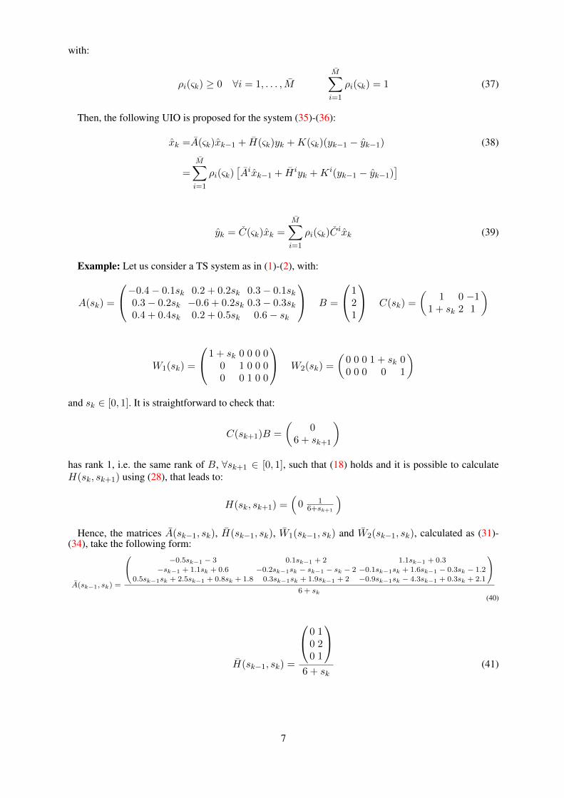
Example: Let us consider a TS system as in (1)-(2), with:

A(sk) =

−0.4− 0.1sk 0.2 + 0.2sk 0.3− 0.1sk0.3− 0.2sk −0.6 + 0.2sk 0.3− 0.3sk0.4 + 0.4sk 0.2 + 0.5sk 0.6− sk

B =

121

C(sk) =

(1 0 −1

1 + sk 2 1

)

W1(sk) =

1 + sk 0 0 0 00 1 0 0 00 0 1 0 0

W2(sk) =

(0 0 0 1 + sk 00 0 0 0 1

)

and sk ∈ [0, 1]. It is straightforward to check that:

C(sk+1)B =

(0

6 + sk+1

)has rank 1, i.e. the same rank of B, ∀sk+1 ∈ [0, 1], such that (18) holds and it is possible to calculateH(sk, sk+1) using (28), that leads to:

H(sk, sk+1) =(

0 16+sk+1

)Hence, the matrices A(sk−1, sk), H(sk−1, sk), W1(sk−1, sk) and W2(sk−1, sk), calculated as (31)-

(34), take the following form:

A(sk−1, sk) =

−0.5sk−1 − 3 0.1sk−1 + 2 1.1sk−1 + 0.3

−sk−1 + 1.1sk + 0.6 −0.2sk−1sk − sk−1 − sk − 2 −0.1sk−1sk + 1.6sk−1 − 0.3sk − 1.20.5sk−1sk + 2.5sk−1 + 0.8sk + 1.8 0.3sk−1sk + 1.9sk−1 + 2 −0.9sk−1sk − 4.3sk−1 + 0.3sk + 2.1

6 + sk

(40)

H(sk−1, sk) =

0 10 20 1

6 + sk

(41)

7

W1(sk−1, sk) =

5 + 5sk−1 −2 −1 0 0−2sk−1sk 2 + sk −2 0 0

−sk−1sk − sk−1 − sk − 1 −2 5 + sk 0 0

6 + sk

(42)

W2(sk−1, sk) =

0 0 0 0 10 0 0 0 20 0 0 0 1

6 + sk

(43)

By defining the new premise variables ς1 = sk−1, ς2 = sk and ς3 = 16+sk

, and considering thatς1 ∈ [0, 1], ς2 ∈ [0, 1] and ς3 ∈ [1/7, 1/6], (35)-(36) becomes a set of M = 8 subsystems, with thefollowing matrices

A1 =

−0.4286 0.2857 0.04290.0857 −0.2857 −0.17140.2571 0.2857 0.3000

A2 =

−0.5000 0.3333 0.05000.1000 −0.3333 −0.20000.3000 0.3333 0.3500

A3 =

−0.4286 0.2857 0.04290.2429 −0.4286 −0.21430.3714 0.2857 0.3429

A4 =

−0.5000 0.3333 0.05000.2833 −0.5000 −0.25000.4333 0.3333 0.4000

A5 =

−0.5000 0.3000 0.2000−0.0571 −0.4286 0.05710.6143 0.5571 −0.3143

A6 =

−0.5833 0.3500 0.2333−0.0667 −0.5000 0.06670.7167 0.6500 −0.3667

A7 =

−0.5000 0.3000 0.20000.1000 −0.6000 00.8000 0.6000 −0.4000

A8 =

−0.5833 0.3500 0.23330.1167 −0.7000 00.9333 0.7000 −0.4667

H1 = H3 = H5 = H7 =

0 0.14290 0.28570 0.1429

H2 = H4 = H6 = H8 =

0 0.16670 0.33330 0.1667

W 11 =

0.7143 −0.2857 −0.1429 0 0−0.2857 0.2857 −0.2857 0 0−0.1429 −0.2857 0.7143 0 0

W 21 =

0.8333 −0.3333 −0.1667 0 0−0.3333 0.3333 −0.3333 0 0−0.1667 −0.3333 0.8333 0 0

W 31 =

0.7143 −0.2857 −0.1429 0 0−0.5714 0.4286 −0.2857 0 0−0.2857 −0.2857 0.8571 0 0

W 41 =

0.8333 −0.3333 −0.1667 0 0−0.6667 0.5000 −0.3333 0 0−0.3333 −0.3333 1.0000 0 0

8

W 51 =

1.4286 −0.2857 −0.1429 0 0−0.5714 0.2857 −0.2857 0 0−0.2857 −0.2857 0.7143 0 0

W 61 =

1.6667 −0.3333 −0.1667 0 0−0.6667 0.3333 −0.3333 0 0−0.3333 −0.3333 0.8333 0 0

W 71 =

1.4286 −0.2857 −0.1429 0 0−1.1429 0.4286 −0.2857 0 0−0.5714 −0.2857 0.8571 0 0

W 81 =

1.6667 −0.3333 −0.1667 0 0−1.3333 0.5000 −0.3333 0 0−0.6667 −0.3333 1.0000 0 0

W 12 = W 3

2 = W 52 = W 7

2 =

0 0 0 0 0.14290 0 0 0 0.28570 0 0 0 0.1429

W 22 = W 4

2 = W 62 = W 8

2 ==

0 0 0 0 0.16670 0 0 0 0.33330 0 0 0 0.1667

C12 = C2

2 = C52 = C6

2 =

(1 0 −11 2 1

)C3

2 = C42 = C7

2 = C82 =

(1 0 −12 2 1

)

W 12 = W 2

2 = W 52 = W 6

2 =

(0 0 0 1 00 0 0 0 1

)W 3

2 = W 42 = W 7

2 = W 82 =

(0 0 0 2 00 0 0 0 1

)

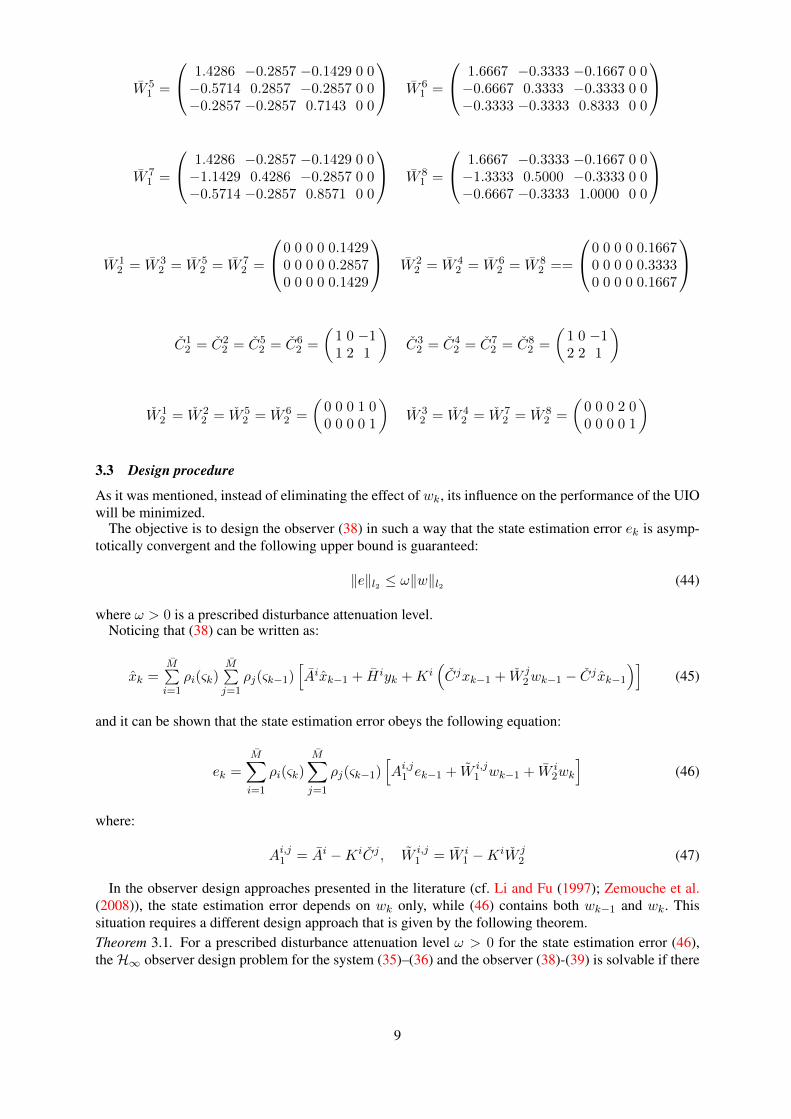
3.3 Design procedure

As it was mentioned, instead of eliminating the effect of wk, its influence on the performance of the UIOwill be minimized.

The objective is to design the observer (38) in such a way that the state estimation error ek is asymp-totically convergent and the following upper bound is guaranteed:

‖e‖l2 ≤ ω‖w‖l2 (44)

where ω > 0 is a prescribed disturbance attenuation level.Noticing that (38) can be written as:

xk =M∑i=1

ρi(ςk)M∑j=1

ρj(ςk−1)[Aixk−1 + H iyk +Ki

(Cjxk−1 + W j

2wk−1 − Cj xk−1

)](45)

and it can be shown that the state estimation error obeys the following equation:

ek =

M∑i=1

ρi(ςk)

M∑j=1

ρj(ςk−1)[Ai,j1 ek−1 + W i,j

1 wk−1 + W i2wk

](46)

where:

Ai,j1 = Ai −KiCj , W i,j1 = W i

1 −KiW j2 (47)

In the observer design approaches presented in the literature (cf. Li and Fu (1997); Zemouche et al.(2008)), the state estimation error depends on wk only, while (46) contains both wk−1 and wk. Thissituation requires a different design approach that is given by the following theorem.Theorem 3.1. For a prescribed disturbance attenuation level ω > 0 for the state estimation error (46),theH∞ observer design problem for the system (35)–(36) and the observer (38)-(39) is solvable if there

9

exist matrices P i � 0, N i (i = 1, . . . , M ) and U such that the following inequality is satisfied for alli, j, l = 1, . . . , M :

Υli,j =

I − P i 0 0 (Ai,j1 )TUT

0 −µ2I 0 (W i,j1 )TUT

0 0 −µ2I (W i2)TUT

UAi,j1 UW i,j1 UW i

2 Pl − U − UT

≺ 0 (48)

with µ = ω/√

2 and:

UAi,j1 = UAi − UKiCj = UAi −N iCj (49)

UW i,j1 = UW i

1 − UKiW j2 = UW i

1 −N iW j2 . (50)

Proof. The problem of H∞ observer design (Li and Fu 1997; Zemouche et al. 2008) is to determine thematrices Ki, i = 1, . . . , M such that

limk→∞

ek = 0 for wk = 0 ∀k (51)

‖e‖l2 ≤ ω‖w‖l2 for wk 6= 0, e0 = 0. (52)

In this paper, a quadratic Lyapunov approach is used, which means that it is sufficient to find a functionVk � 0 such that:

∆Vk−1 + eTk−1ek−1 − µ2wTk−1wk−1 − µ2wTk wk < 0, k = 1, . . . ,∞ (53)

where ∆Vk−1 = Vk − Vk−1, µ > 0. Indeed, if wk = 0, k = 1, . . . ,∞, then (53) can be expressed as:

∆Vk−1 + eTk−1ek−1 < 0, k = 1, . . .∞ (54)

and hence ∆Vk−1 < 0, which leads to (51). If wk 6= 0, k = 1, . . . ,∞, then (53) yields:

J =

∞∑k=1

(∆Vk−1 + eTk−1ek−1 − µ2wTk−1wk−1 − µ2wTk wk

)< 0 (55)

which can be written as:

J = −V0 +

∞∑k=1

eTk−1ek−1 − µ2∞∑k=1

wTk−1wk−1 − µ2∞∑k=1

wTk wk < 0 (56)

Bearing in mind that:

µ2∞∑k=1

wTk wk = µ2∞∑k=1

wTk−1wk−1 − µ2wT0 w0 (57)

the inequality (56) can be written as:

J = −V0 +

∞∑k=1

eTk−1ek−1 − 2µ2∞∑k=1

wTk−1wk−1 + µ2wT0 w0 < 0 (58)

Knowing that V0 = 0 for e0 = 0, (58) leads to (52) with ω =√

2µ.

10

Let us consider the following form for the Lyapunov function:

Vk =

M∑i=1

ρi(ςk)eTk P

iek, P i � 0 (59)

Thus, by defining vk−1 = [eTk−1, wTk−1, w

Tk ], it can be shown that the condition (53) is equivalent to:

M∑i=1

ρi(ςk−1)

M∑j=1

ρj(ςk)

M∑l=1

ρl(ςk)vTk−1Φl

i,jvk−1 < 0 (60)

where:

Φli,j =

(Ai,j1 )TP lAi,j

1 + I − P i (Ai,j1 )TP lW i,j

1 (Ai,j1 )TP lW i

2

(W i,j1 )TP lAi,j

1 (W i,j1 )TP lW i,j

1 − µ2I (W i,j1 )TP lW i

2

(W i2)TP lAi,j

1 (W i2)TP lW i,j

1 (W i2)TP lW i

2 − µ2I

(61)

Let us remind the following lemma (de Oliveira et al. 1999):Lemma 3.1. The following statements are equivalent:

(1) There exists X � O such that

Y TXY −W ≺ O (62)

(2) There exists X � O such that [−W Y TUT

UY X − U − UT]≺ O. (63)

Applying Lemma 3.1 to (61) leads to (48), which completes the proof. �

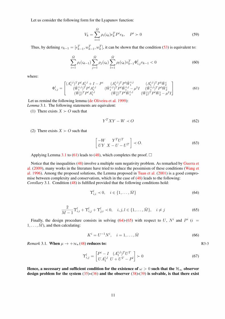
Notice that the inequalities (48) involve a multiple sum negativity problem. As remarked by Guerra etal. (2009), many works in the literature have tried to reduce the pessimism of these conditions (Wang etal. 1996). Among the proposed solutions, the Lemma proposed in Tuan et al. (2001) is a good compro-mise between complexity and conservatism, which in the case of (48) leads to the following:Corollary 3.1. Condition (48) is fulfilled provided that the following conditions hold:

Υli,i ≺ 0, i ∈ {1, . . . , M} (64)

2

M − 1Υli,i + Υl

i,j + Υlj,i ≺ 0, i, j, l ∈ {1, . . . , M}, i 6= j (65)

Finally, the design procedure consists in solving (64)-(65) with respect to U , N i and P i (i =1, . . . , M ), and then calculating:

Ki = U−1N i, i = 1, . . . , M (66)

Remark 3.1. When µ→ +∞, (48) reduces to: R3-3

Υli,j =

[P i − I (Ai,j1 )TUT

UAi,j1 U + UT − P l

]� 0 (67)

Hence, a necessary and sufficient condition for the existence of ω > 0 such that the H∞ observerdesign problem for the system (35)–(36) and the observer (38)-(39) is solvable, is that there exist

11

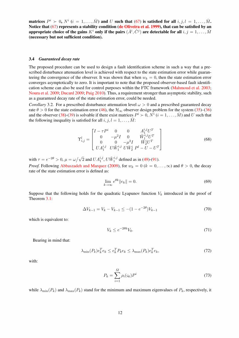
matrices P i � 0, N i (i = 1, . . . , M ) and U such that (67) is satisfied for all i, j, l = 1, . . . , M .Notice that (67) represents a stability condition (de Oliveira et al. 1999), that can be satisfied by anappropriate choice of the gains Ki only if the pairs (Ai, Cj) are detectable for all i, j = 1, . . . , M(necessary but not sufficient condition).

3.4 Guaranteed decay rate

The proposed procedure can be used to design a fault identification scheme in such a way that a pre-scribed disturbance attenuation level is achieved with respect to the state estimation error while guaran-teeing the convergence of the observer. It was shown that when wk = 0, then the state estimation errorconverges asymptotically to zero. It is important to note that the proposed observer-based fault identifi-cation scheme can also be used for control purposes within the FTC framework (Mahmoud et al. 2003;Noura et al. 2009; Ducard 2009; Puig 2010). Thus, a requirement stronger than asymptotic stability, suchas a guaranteed decay rate of the state estimation error, could be needed.Corollary 3.2. For a prescribed disturbance attenuation level ω > 0 and a prescribed guaranteed decayrate θ > 0 for the state estimation error (46), the H∞ observer design problem for the system (35)–(36)and the observer (38)-(39) is solvable if there exist matrices P i � 0, N i (i = 1, . . . , M ) and U such thatthe following inequality is satisfied for all i, j, l = 1, . . . , M :

Υli,j =

I − τP i 0 0 Ai,j1 UT

0 −µ2I 0 W i,j1 UT

0 0 −µ2I W i2U

T

UAi,j1 UW i,j1 UW i

2 Pl − U − UT

(68)

with τ = e−2θ > 0, µ = ω/√

2 and UAi,j1 , UW i,j1 defined as in (49)-(91).

Proof. Following Abbaszadeh and Marquez (2009), for wk = 0 (k = 0, . . . ,∞) and θ > 0, the decayrate of the state estimation error is defined as:

limk→∞

eθk‖ek‖ = 0. (69)

Suppose that the following holds for the quadratic Lyapunov function Vk introduced in the proof ofTheorem 3.1:

∆Vk−1 = Vk − Vk−1 ≤ −(1− e−2θ)Vk−1 (70)

which is equivalent to:

Vk ≤ e−2θkV0. (71)

Bearing in mind that:

λmin(Pk)eTk ek ≤ eTk Pkek ≤ λmax(Pk)e

Tk ek, (72)

with:

Pk =

M∑i=1

ρi(ςk)Pi (73)

while λmin(Pk) and λmax(Pk) stand for the minimum and maximum eigenvalues of Pk, respectively, it

12

can be shown that:

‖ek‖ ≤

√λmax(P0)

λmin(Pk)e−θk‖e0‖, (74)

which is equivalent to (69).Thus, using (70), to attain a guaranteed decay rate θ it is needed that:

∆Vk−1 ≤ −(1− e−2θ)Vk = −(1− e−2θ)eTk Pkek, (75)

which is equivalent to replacing −P i in (48) by −τP i (τ = e−2θ, i.e. θ = −12 ln(τ)), which gives (68),

completing the proof. �

Hence, given a prescribed disturbance attenuation level ω, the following optimisation problem can beformulated:

τ∗ = minτ>0,P i�0,N i,U

τ (76)

subject to (64) and (65).An alternative solution is to minimize µ and τ simultaneously, i.e., given a scalar 0 ≤ λ ≤ 1 the

optimization problem is (cf. Abbaszadeh and Marquez (2009)):

(τ∗, µ∗) = minτ>0,µ,P i�0,N i,U

λτ + (1− λ)µ (77)

subject to (64) and (65).These minimization problems involve bilinear matrix inequalities (BMIs) due to the products of τ by

P i. However, a line search approach allows to solve it using LMI solvers.

3.5 Fault estimation strategySince the design procedure of the UIO is provided, it is possible to propose a fault estimation strategythat is based on the obtained state estimates. For that purpose, let us rewrite the system (1)-(2) as follows:

xk+1 = A(sk)xk +B(sk)uk +B(sk)fk +W1(sk)wk (78)

yk+1 = C(sk+1)xk+1 +W2(sk+1)wk+1 (79)

Taking into account that the rank condition (18) holds, it is possible to calculate the matrixH(sk, sk+1), as in (28). Then, pre-multiplying (79) by H(sk, sk+1) and replacing in it (78), the fol-lowing is obtained:

fk = H(sk, sk+1)[yk+1 − C(sk+1)A(sk)xk − C(sk+1)W1(sk)wk −W2(sk+1)wk+1]− uk. (80)

Thus, the fault estimate is given by:

fk = H(sk, sk+1)[yk+1 − C(sk+1)A(sk)xk]− uk. (81)

3.6 Observer design with unmeasurable premise variablesLet us consider the case where the premise variables are partially or completely unmeasured. In thiscase, the assumption that Ci = C and W i

2 = W2, i = 1, . . . , M , is done. Then, the UIO (38)-(39) is

13

slightly modified, as follows:

xk =A(ςk)xk−1 + H(ςk)yk +K(ςk)(yk−1 − yk−1) (82)

=

M∑i=1

ρi(ςk)[Aixk−1 + H iyk +Ki(yk−1 − yk−1)

]

yk = Cxk (83)

where ςk is an estimation of ςk.Then, taking into account (1)-(2), the estimation error obeys the following equation:

ek =(A(ςk)−K(ςk)C

)ek−1 +

(W1(ςk)−K(ςk)W2

)wk−1 + W2(ςk)wk + ∆(·) (84)

=

M∑i=1

ρi(ςk)[Ai1ek−1 + W i

1wk−1 + W i2wk

]+ ∆(·)

where:

Ai1 = Ai −KiC, W i1 = W i

1 −KiW2 (85)

and ∆(·) is given by:

∆(·) =(A(ςk)− A(ςk)

)xk−1 +

(H(ςk)− H(ςk)

)yk +

(W1(ςk)− W1(ςk

)wk−1 +

(W2(ςk)− W2(ςk

)wk

=

M∑i=1

(ρi(ςi)− ρi(ςi))[Aixk−1 + Hiyk + W i

1wk−1 + W i2wk

](86)

Assumption 1: ∆(·) is one-sided Lipschitz (Zhang et al. 2012) in ek, i.e. there exists ρ ∈ R such that,for an arbitrary ek ∈ Rn:

〈∆(·), ek〉 ≤ ρ ‖ek‖2 (87)

where 〈·, ·〉 denotes the inner product, and ρ ∈ Rn is called the one-sided Lipschitz constant, which canbe positive, zero, or even negative.

Assumption 2: ∆(·) is quadratic inner-bounded (Zhang et al. 2012) in ek−1, i.e. for an arbitrary ek−1 ∈Rn, there exist σ, ϕ ∈ R such that:

∆(·)T∆(·) ≤ σ ‖ek−1‖2 + ϕ 〈ek−1,∆(·)〉 (88)

Notice that the properties of one-sided Lipschitz and quadratic inner-boundedness include the Lips-chitz property as a particular case2.

The discussion in Zhang et al. (2012) has shown that, under the setting of Lipschitz nonlinearities, itis difficult to design observers in the case of Lipschitz constant bigger than one. This fact has motivatedthe observer design for one-sided Lipschitz systems, with the aim of reducing the conservatism of theresults.Corollary 3.3. Assume that ∆(·), defined as in (86), satisfies conditions (87)-(88) with constants ρ, σand ϕ. Then, for a prescribed disturbance attenuation level ω > 0 and a prescribed guaranteed decay

2In practice, it is not required that these properties hold ∀ek−1, ek ∈ Rn, but only for values that are reasonable taking into account thesystem’s characteristics and sensors.

14

rate θ > 0 for the state estimation error (84), the H∞ observer design problem for the system (35)–(36)with Ci = C and W i

2 = W2, i = 1, . . . , M , and the observer (82)-(83) is solvable if there exist matricesP i � 0, N i (i = 1, . . . , M ) and U such that the following inequality is satisfied for all i, l = 1, . . . , M :

Υli,j =

I − τP i + ε1ρI + ε2σI 0 0 ϕε2−ε1

2 I Ai1UT

0 −µ2I 0 0 W i1U

T

0 0 −µ2I 0 W i2U

T

ϕε2−ε12 I 0 0 −ε2I UT

UAi1 UW i1 UW i

2 U P l − U − UT

(89)

with τ = e−2θ > 0, µ = ω/√

2 and UAi1, UW i1 defined as:

UAi1 = UAi − UKiC = UAi −N iC (90)

UW i1 = UW i

1 − UKiW2 = UW i1 −N iW2. (91)

Proof. Let us consider the following Lyapunov function:

Vk =

M∑i=1

ρi(ςk)eTk P

iek, P i � 0 (92)

and let us assume that (70) holds (see proof of Corollary 3.2). Then, by defining vk−1 =[eTk−1, w

Tk−1, w

Tk ,∆(·)T ], it can be shown that the condition (70) is equivalent to:

M∑i=1

ρi(ςk−1)

M∑l=1

ρl(ςk)vTk−1Φl

ivk−1 < 0 (93)

where:

Φli =

(Ai

1)TP lAi1 + I − τP i (Ai

1)TP lW i1 (Ai

1)TP lW i2 (Ai

1)TP l

(W i1)TP lAi

1 (W i1)TP lW i

1 − µ2I (W i1)TP lW i

2 (W i1)TP l

(W i2)TP lAi

1 (W i2)TP lW i

1 (W i2)TP lW i

2 − µ2I (W i2)TP l

P lAi1 P lW i

1 P lW i2 P l

(94)

From (87), we get ρeTk ek − eTk ∆(·) ≥ 0. Therefore, for any ε1 > 0:

ε1

[ek−1

∆(·)

]T [ρI − I

2− I

2 −I

] [ek−1

∆(·)

]≥ 0 (95)

Similarly, from (88), we have for any ε2 > 0:

ε2

[ek−1

∆(·)

]T [σI ϕI

2ϕI2 −I

] [ek−1

∆(·)

]≥ 0 (96)

By combining (93)-(94) with (95)-(96), the following is obtained:

Φli =

(Ai

1)TP lAi1 + I − τP i + ε1ρI + ε2σI (Ai

1)TP lW i1 (Ai

1)TP lW i2 (Ai

1)TP l + ϕε2−ε12 I

(W i1)TP lAi

1 (W i1)TP lW i

1 − µ2I (W i1)TP lW i

2 (W i1)TP l

(W i2)TP lAi

1 (W i2)TP lW i

1 (W i2)TP lW i

2 − µ2I (W i2)TP l

P lAi1 + ϕε2−ε1

2 I P lW i1 P lW i

2 P l − ε2I

≺ 0

(97)

15

Applying Lemma 3.1 to (97) leads to (89), which completes the proof. �

4. Illustrative examples

4.1 Academic example

Let us consider the TS system provided in the example at the end of Section 3.2, and let us notice thatthe approach proposed by Chadli and Karimi (2013) cannot be applied to this example, since (15) leadsto E = 0 which, combined with (11) and (14), gives:

TBi −KiF = Bi = 0 (98)

which is false. On the other hand, applying the design procedure described in Section 3.3, the followingUIO matrices are obtained with µ = 4.6615:

K1 =

−0.4473 0.12260.1880 −0.13240.0788 0.1570

K2 =

−0.5237 0.13830.2313 −0.14310.0790 0.1685

K3 =

−0.4872 0.10390.4589 −0.16510.0063 0.1620

K4 =

−0.5657 0.09920.5328 −0.16930.0164 0.1855

K5 =

−0.5416 0.12050.1190 −0.16160.3205 0.2266

K6 =

−0.6522 0.12730.1654 −0.17080.3576 0.2639

K7 =

−0.5802 0.08600.4185 −0.16610.2673 0.2233

K8 =

−0.6246 −0.02640.5515 −0.04030.3749 0.2220

In order to show the performance of the proposed approach, a simulation has been performed with

x0 = (5,−5, 2)T , uk = sin(k/20), wi ∈ [−0.1, 0.1], i = 1, . . . , 5, where each wi is generated as arandom sequence, s ∈ [0, 1] as shown in Figure 1 (corresponding to the activation functions ρi, i =1, . . . , 8, depicted in Figure 2), and fk as follows:

fk =

0 k ≤ 200.5 20 < k ≤ 40

0.5 + 0.5 sin(2πk/40) else

As expected, the results shown in Figures 3 and 4 demonstrate the convergence of the UIO in theestimation of both the state xk and the fault fk, thus proving the effectiveness of the developed method.

4.2 Multi-tank system

Let us consider a multi-tank system portrayed in Fig. 5. It consists of three separate tanks placedR2-1 R3-4one above the other and equipped with drain valves and level sensors based on hydraulic pressuremeasurement (Witczak 2014). Each of them has a different cross-section in order to reflect systemnonlinearities. The lower bottom tank is a water reservoir for the system. A variable speed wa-ter pump is used to fill the upper tank and the water outflows the tanks due to the gravity. The

16

0 20 40 60 80 1000

0.1

0.2

0.3

0.4

0.5

0.6

0.7

0.8

0.9

Sample k

s(k)

Figure 1. Premise variable s(k).

0 50 1000

0.05

0.1

0.15

0.2

ρ 1(ςk)

0 50 1000

0.5

1

ρ 2(ςk)

0 50 1000

0.05

0.1

0.15

0.2ρ 3(ς

k)

0 50 1000

0.05

0.1

0.15

0.2

ρ 4(ςk)

0 50 1000

0.05

0.1

0.15

0.2

ρ 5(ςk)

Sample k0 50 100

0

0.05

0.1

0.15

0.2

ρ 6(ςk)

Sample k0 50 100

0

0.05

0.1

0.15

0.2

ρ 7(ςk)

Sample k0 50 100

0

0.05

0.1

0.15

0.2ρ 8(ς

k)

Sample k

Figure 2. Activation functions ρ(k).

nonlinear discrete-time model of the multi-tank system is given by (Witczak 2014):h1(k + 1) = h1(k)− c1h1(k)α + bu(k)

h2(k + 1) = h2(k) + (c3 + c4h2(k))−1 (c2h1(k)α − c5h2(k)α)

h3(k + 1) = h3(k) +(c7 − (c8 − h3(k))2

)−0.5(c6h2(k)α − c9h3(k)α)

(99)

where the real data-based parameters were identified as follows: b = 1.14, α = 0.5, c1 = 1.15·10−4,c2 = 1.01 ·10−6, c3 = 3.5 ·10−3, c4 = 3.48 ·10−2, c5 = 1.20 ·10−6, c6 = 3.42 ·10−5, c7 = 1.33 ·10−1,c8 = 3.5 · 10−1 and c9 = 2.80 · 10−5.

By considering actuator faults fk and an exogenous disturbance vector wk entering into thesystem through the matrix:

W1 =

0.001 0 00 0 00 0 0

17

0 20 40 60 80 100−5

0

5

x 1(k)

0 20 40 60 80 100−5

0

5

x 2(k)

0 20 40 60 80 100−5

0

5

10

Sample k

x 3(k)

realestimation

Figure 3. State xk and its estimation xk using the proposed UIO.

0 20 40 60 80 100−0.2

0

0.2

0.4

0.6

0.8

1

1.2

Sample k

f k

realestimation

Figure 4. Fault fk and its estimation fk using the proposed UIO.

one can rewrite (99) as (1), with xk = [h1(k), h2(k), h3(k)]T , uk = u(k), and:

A(sk) =

s(1)k 0 0

s(2)k s

(3)k 0

0 s(4)k s

(5)k

B =

b00

18

Figure 5. Multi-Tank system.

where:

s(1)k =1− c1h1(k)α−1

s(2)k =c2 (c3 + c4h2(k))−1 h1(k)α−1

s(3)k =1− c5 (c3 + c4h2(k))−1 h2(k)α−1

s(4)k =c6

(c7 − (c8 − h3(k))2

)−0.5h2(k)α−1

s(5)k =1− c9

(c7 − (c8 − h3(k))2

)−0.5h3(k)α−1

It is assumed that noisy measurements of h1(k) and h2(k) are available, i.e., the output equation(2) is characterized by the matrices:

C =

(1 0 00 1 0

)W2 =

(0 0.003 00 0 0.003

)It is easy to check that (18) is verified, since:

CB =

(b0

)has rank 1, which allows calculating H using (28):

H =(

1b 0

)Hence, it follows from (31)-(34) that:

A(sk−1) =

0 0 0

s(2)k−1 s

(3)k−1 0

0 s(4)k−1 s

(5)k−1

H =

1 00 00 0

19

W1 =

0 0 00 0 00 0 0

W2 =

0 0.003 00 0 00 0 0

By defining the new premise variables ς1 = s

(2)k−1, ς2 = s

(3)k−1, ς3 = s

(4)k−1 and ς4 = s

(5)k−1 and

considering that hi ∈ [hmin, hmax], i = 1, 2, 3, (35)-(36) becomes a set of M = 16 subsystems,obtained considering all the possible combinations of extreme values of the intervals [ςmin

i , ςmaxi ],

i = 1, 2, 3, 4, calculated as follows:

ςmin1 = c2 (c3 + c4 + hmax)−1 hα−1

max ςmax1 = c2 (c3 + c4 + hmin)−1 hα−1

min

ςmin2 = 1− c5 (c3 + c4hmin)−1 hα−1

min ςmax2 = 1− c5 (c3 + c4hmax)−1 hα−1

max

ςmin3 = c6

(c7 − (c8 − hmax)2

)−0.5hα−1

max ςmax3 = c6

(c7 − (c8 − hmin)2

)−0.5hα−1

min

ςmin4 = 1− c9

(c7 − (c8 − hmin)2

)−0.5hα−1

min ςmax4 = 1− c9

(c7 − (c8 − hmax)2

)−0.5hα−1

max

Due to the noise and the unavailability of measurements for h3(k), the case of unmeasurablepremise variables should be considered, as described in Section 3.6. In this case, (86) reads asfollows:

∆(·) =

0(

s(2)k − s

(2)k

)h1(k) +

(s

(3)k − s

(3)k

)h2(k)(

s(4)k − s

(4)k

)h2(k) +

(s

(5)k − s

(5)k

)h3(k)

The properties of ∆(·) being one-sided Lipschitz and quadratic inner-bounded, i.e. (87)-(88),

have been verified with ρ = 0.0012, σ = 10−11 and ϕ = 0.2396.Applying the design procedure described in Section 3.6, a feasible solution has been obtained

with τ = 5, µ = 1.35 · 10−3, ε1 = 6.3829 and ε2 = 26.89.All of the experiments have been performed with the real system using the following parameters:

x0 = [0.001, 0.001, 0.001]T , x0 = [0.05, 0.05, 0.01]T , uk = 9 · 10−5, and fk defined as:

fk =

{−0.33 · uk 10001 < k ≤ 15000

0 otherwise

Fig. 6 shows the activation functions ρ(k) of the described system. Figs. 7–9 present the states and theirestimates. Considering that the water level in the third tank is unmeasurable and that it varies in theinterval [0, 0.35 (m)] the results are satisfactory, as it can be clearly observed in Fig. 10 depicting thestate estimation error. Indeed, the estimation error does not exceed 1cm which, taking into account thepermanent water flow as well as the sensor measurement imprecision, should be perceived as a goodresult. Fig. 11 shows the actuator loss of effectiveness fault fk and its robust estimate fk (red dashedline). The obtained results have been compared with the ones obtained using a linear UIO, as proposedby Witczak (2014). In this case, the matrices describing the linear model have been taken from thedocumentation (INTECO 2013). The fault estimation obtained using the linear UIO is shown in Fig. 11(black dashed line). From these results, it is clear that the proposed UIO performs significantly betterthan the linear one. Indeed, Fig. 12 clearly shows that the fault estimation error associated with theproposed approach is relatively small.

20

0 0.5 1 1.5 2 2.5

x 104

0

0.5

1

ρ 1(ςk)

0 0.5 1 1.5 2 2.5

x 104

0

0.5

1

ρ 2(ςk)

0 0.5 1 1.5 2 2.5

x 104

0

0.5

1

ρ 3(ςk)

0 0.5 1 1.5 2 2.5

x 104

0

0.5

1

ρ 4(ςk)

0 0.5 1 1.5 2 2.5

x 104

0

0.5

1

ρ 5(ςk)

0 0.5 1 1.5 2 2.5

x 104

0

0.5

1

ρ 6(ςk)

0 0.5 1 1.5 2 2.5

x 104

0

0.5

1

ρ 7(ςk)

0 0.5 1 1.5 2 2.5

x 104

0

0.5

1

ρ 8(ςk)

0 0.5 1 1.5 2 2.5

x 104

0

0.5

1

ρ 9(ςk)

0 0.5 1 1.5 2 2.5

x 104

0

0.5

1

ρ 10(ς

k)0 0.5 1 1.5 2 2.5

x 104

0

0.5

1

ρ 11(ς

k)

0 0.5 1 1.5 2 2.5

x 104

0

0.5

1

ρ 12(ς

k)

0 0.5 1 1.5 2 2.5

x 104

0

0.5

1

ρ 13(ς

k)

Sample k0 0.5 1 1.5 2 2.5

x 104

0

0.5

1

ρ 14(ς

k)

Sample k0 0.5 1 1.5 2 2.5

x 104

0

0.5

1

ρ 15(ς

k)

Sample k0 0.5 1 1.5 2 2.5

x 104

0

0.5

1

ρ 16(ς

k)

Sample k

Figure 6. Activation functions ρ(k).

0 0.5 1 1.5 2 2.5

x 104

0

0.05

0.1

0.15

0.2

0.25

0.3

Sample k

x 1(k)

realestimation

0 50 1000

0.005

0.01

Figure 7. State x1,k and its estimate using the proposed UIO - first tank.

5. Conclusions

In this paper, an UIO for TS systems has been proposed, with the goal of jointly estimating the stateand the unknown actuator faults. Differently from recent results appeared in the literature, the proposedapproach can deal with TS systems whose output equation matrices are not constant. Moreover, insteadof eliminating the external disturbances, their influence on the UIO performance is minimized, with theadvantage of not requiring the perfect knowledge of the disturbance distribution matrices. The wholedesign procedure, that aims at achieving convergence of the estimation error either with any rate, or witha guaranteed decay rate, boils down to solve a set of LMIs, a problem that can be efficiently solved usingthe solvers available nowadays. The case of activation functions which depend on unmeasurable premisevariables has been also considered. The effectiveness of the proposed method has been demonstratedusing an academical example and a real system application. In particular, a multi-tank system was em-ployed to perform a comparison of the proposed TS UIO with a linear one. The obtained results clearlyshow that the proposed approach performs significantly better than the linear one.

21

0 0.5 1 1.5 2 2.5

x 104

0

0.02

0.04

0.06

0.08

0.1

0.12

0.14

0.16

Sample k

x 2(k)

realestimation

0 50 1000

0.005

0.01

Figure 8. State x2,k and its estimate using the proposed UIO - second tank.

0 0.5 1 1.5 2 2.5

x 104

0

0.02

0.04

0.06

0.08

0.1

0.12

0.14

Sample k

x 3(k)

realestimation

0 50 1000

0.005

0.01

Figure 9. State x3,k and its estimate using the proposed UIO - third tank.

Acknowledgments

This work has been funded by the National Science Centre in Poland under the grant2013/11/B/ST7/01110, by the Spanish Government (MINECO) through the project CICYT ECOCIS(ref. DPI2013-48243-C2-1-R), by MINECO and FEDER through the project CICYT HARCRICS (ref.DPI2014-58104-R), by AGAUR through the contracts FI-DGR 2014 (ref. 2014FI_B1 00172) and FI-DGR 2015 (ref. 2015FI_B2 00171), and by the DGR of Generalitat de Catalunya (SAC group Ref.2014/SGR/374).

References

Abbaszadeh, M., and Marquez, H.J. (2009), “LMI optimization approach to robustH∞ observer design and staticoutput feedback stabilization for discrete-time nonlinear uncertain systems,” International Journal of Robustand Nonlinear Control, 19(3), 313–340.

Bouattour, M., Chadli, M., El Hajjaji, A., and Chaabane, M. (2010), “Estimation of state, actuator and sensor faultsfor TS models,” in Proceedings of the 49th IEEE Conference on Decision and Control (CDC), pp. 1613–1618.

Brahim, A., Dhahri, S., Hmida, F., and Sellami, A. (2015), “An H∞ sliding mode observer for Takagi–Sugeno

22

0 0.5 1 1.5 2 2.5

x 104

−0.01

−0.008

−0.006

−0.004

−0.002

0

0.002

0.004

0.006

0.008

0.01

Sample k

Sta

te x

3 est

imat

ion

erro

r

Figure 10. State estimation error using the proposed UIO - third tank.

0 0.5 1 1.5 2 2.5

x 104

−1.5

−1

−0.5

0

0.5

1

1.5x 10

−4

Sample k

F(k

)

realestimationlinear estimation

Figure 11. Fault fk and its estimation fk using the proposed and linear UIO.

nonlinear systems with simultaneous actuator and sensor faults,” International Journal of Applied Mathematicsand Computer Science, 25(3), 547–559.

Chadli, M. (2010), “An LMI approach to design observer for unknown inputs Takagi-Sugeno fuzzy models,” AsianJournal of Control, 12(4), 524–530.

Chadli, M., Akhenak, A., Ragot, J., and Maquin, D. (2009), “State and unknown input estimation for discrete timemultiple model,” Journal of the Franklin Institute, 346(6), 593–610.

Chadli, M., and Karimi, H.R. (2013), “Robust observer design for unknown inputs Takagi-Sugeno models,” IEEETransactions on Fuzzy Systems, 21(1), 158–164.

Chen, W., and Saif, M. (2007), “Design of a TS based fuzzy nonlinear unknown input observer with fault diagnosisapplication,” in Proceedings of the 24th American Control Conference, pp. 2545–2550.

Chen, W., and Saif, M. (2010), “Fuzzy nonlinear unknown input observer design with fault diagnosis applications,”Journal of Vibration and Control, 16(3), 377–401.

Cotton, N.J., and Wilamowski, B.M. (2010), “Compensation of sensors nonlinearity with neural networks,” inProceedings of the 24th IEEE International Conference on Advanced Information Networking and Applications,pp. 1210–1217.

de Oliveira, M.C., Bernussou, J., and Geromel, J.C. (1999), “A new discrete-time robust stability condition,” Sys-tems and Control Letters, 37(4), 261–265.

Ducard, G., Fault-tolerant flight control and guidance systems: practical methods for small unmanned aerial vehi-

23

0 0.5 1 1.5 2 2.5

x 104

−4

−3

−2

−1

0

1

2

3

4x 10

−5

Sample k

Fau

lt es

timat

ion

erro

r

Figure 12. Fault estimation error using the proposed UIO.

cles, Berlin: Springer-Verlag (2009).Elsner, L., Monov, V., and Szulc, T. (2002), “On some properties of convex matrix sets characterized by P-matrices

and block P-matrices,” Linear and Multilinear Algebra, 50, 199–218.Elsner, L., and Szulc, T. (1998), “Convex combinations of matrices - nonsingularity and Schur stability characteri-

zations,” Linear and Multilinear Algebra, 44, 301–312.Elsner, L., and Szulc, T. (2002), “Convex sets of Schur stable and stable matrices,” Linear and Multilinear Algebra,

48, 1–19.Feng, G. (2006), “A survey on analysis and design of model-based fuzzy control systems,” IEEE Transactions on

Fuzzy Systems, 14(5), 676–697.Fonod, R., Henry, D., Charbonnel, C., and Bornschlegl, E. (2014), “A class of nonlinear unknown input observer

for fault diagnosis: application to fault tolerant control of an autonomous spacecraft,” in Proceedings of the 10thUKACC International Conference on Control, pp. 19–24.

Gillijns, S., and Moor, B.D. (2007), “Unbiased minimum-variance input and state estimation for linear discrete-time systems with direct feedthrough,” Automatica, 43(5), 934–937.

Guerra, T.M., Kruszewski, A., and Lauber, J. (2009), “Discrete Takagi-Sugeno models for control: where are we?,”Annual Reviews in Control, 33(1), 37–47.

Hwang, I., Kim, S., Kim, Y., and Seah, C.E. (2010), “A survey of fault detection, isolation, and reconfigurationmethods,” IEEE Transactions on Control Systems Technology, 18(3), 636–653.

Ichalal, D., Marx, B., Ragot, J., and Maquin, D. (2009), “An approach for the state estimation of Takagi-Sugenomodels and application to sensor fault diagnosis,” in Proceedings of the 48th IEEE Conference on Decision andControl (CDC), pp. 7789–7794.

Ichalal, D., Marx, B., Ragot, J., and Maquin, D. (2010), “State estimation of Takagi-Sugeno systems with unmea-surable premise variables,” IET Control Theory and Applications, 4(5), 897–908.

INTECO„ Multitank System - User’s manual, www.inteco.com.pl (2013).Jia, Q.X., Zhang, Y.C., Guan, Y., and Wu, L.N. (2011), “Robust nonlinear unknown input observer-based fault

diagnosis for satellite attitude control system,” in Proceedings of the 10th UKACC International Conference onControl, pp. 345–350.

Johansen, T.A., Shorten, R., and Murray-Smith, R. (2000), “On the interpretation and identification of dynamicTakagi-Sugeno models,” IEEE Transactions on Fuzzy Systems, 8(3), 297–313.

Johnson, C.R., and Tsatsomeros, M.J. (1995), “Convex sets of nonsingular and P-matrices,” Linear and MultilinearAlgebra, 38, 233–239.

K. Zhang, B.J., and Shi, P. (2009), “A new approach to observer-based fault-tolerant controller design for Takagi-Sugeno fuzzy systems with state delay,” Circuits, Systems and Signal Processing, 28(5), 679–697.

Keller, J.Y., and Darouach, M. (1999), “Two-stage Kalman estimator with unknown exogenous inputs,” Automat-ica, 35(2), 339–342.

Kolodziejczak, B., and Szulc, T. (1999), “Convex combinations of matrices - Full rank characterization,” LinearAlgebra and its Applications, 287(1-3), 215–222.

24

Li, H., and Fu, M. (1997), “A linear matrix inequality approach to robust H∞ filtering,” IEEE Transactions onSignal Processing, 45(9), 2338–2350.

Mahmoud, M., Jiang, J., and Zhang, Y., Active fault tolerant control systems, Berlin: Springer-Verlag (2003).Moodi, H., and Farrokhi, M. (2013), “Robust observer design for Sugeno systems with incremental quadratic

nonlinearity in the consequent,” International Journal of Applied Mathematics and Computer Science, 23(4),711–723.

Noura, H., Theilliol, D., Ponsart, J.C., and Chamseddine, A., Fault-tolerant control systems: design and practicalapplications, Berlin: Springer-Verlag (2009).

Patan, K., Witczak, M., and Korbicz, J. (2008), “Towards robustness in neural network based fault diagnosis,”International Journal of Applied Mathematics and Computer Science, 18(4), 443–454.

Puig, V. (2010), “Fault diagnosis and fault tolerant control using set-membership approaches: application to realcase studies,” International Journal of Applied Mathematics and Computer Science, 20(4), 619–635.

Rotondo, D., Puig, V., Nejjari, F., and Witczak, M. (2015), “Automated generation and comparison of Takagi-Sugeno and polytopic quasi-LPV models,” Fuzzy Sets and Systems, 277, 44–64.

Rotondo, D., Reppa, V., Puig, V., and Nejjari, F. (2014), “Adaptive observer for switching linear parameter-varying(LPV) systems,” in Preprints of the 19th IFAC World Congress, pp. 1471–1476.

Samy, I., Postlethwaite, I., and Gu, D.W. (2011), “Survey and application of sensor fault detection and isolationschemes,” Control Engineering Practice, 19(7), 658–674.

Simani, S., Fantuzzi, C., and Patton, R., Model-based fault diagnosis in dynamic systems, Springer, London (2003).Takagi, T., and Sugeno, M. (1985), “Fuzzy identification of systems and its application to modeling and control,”

IEEE Transactions on Systems, Man, and Cybernetics, SMC-15, 116–132.Tanaka, K., and Wang, H.O., Fuzzy control systems design and analysis: a LMI approach, New York: Wiley (2001).Tuan, H.D., Apkarian, P., Narikiyo, T., and Yamamoto, Y. (2001), “Parameterized linear matrix inequality tech-

niques in fuzzy control system design,” IEEE Transactions on Fuzzy Systems, 9(2), 324–332.Vizer, D., Mercere, G., Prot, O., and Ramos, J. (2013), “A local approach for black-box and gray-box LPV system

identification,” in Proceedings of the 12th European Control Conference, pp. 1916–1921.Wang, H.O., Tanaka, K., and Griffin, M.F. (1996), “An approach to fuzzy control of nonlinear systems: stability

and design issues,” IEEE Transactions on Fuzzy Systems, 4(1), 14–23.Wang, S.H., Wang, E., and Dorato, P. (1975), “Observing the states of systems with unmeasurable disturbances,”

IEEE Transactions on Automatic Control, 20(5), 716–717.Witczak, M., Modelling and estimation strategies for fault diagnosis of non-linear systems: from analytical to soft

computing approaches, Berlin: Springer-Verlag (2007).Witczak, M., Fault diagnosis and fault-tolerant control strategies for non-linear systems, Springer (2014).Witczak, M., Buciakowski, M., Puig, V., Rotondo, D., and Nejjari, F. (2015), “An LMI approach to robust fault

estimation for a class of nonlinear systems,” International Journal of Robust and Nonlinear Control.Witczak, M., Rotondo, D., Puig, V., and Witczak, P. (2015), “A practical test for assessing the reachability of

discrete-time Takagi–Sugeno fuzzy systems,” Journal of the Franklin Institute, 352(12), 5936–5951.Xu, D., Jiang, B., and Shi, P. (2012), “Nonlinear actuator fault estimation observer: an inverse system approach via

T-S fuzzy model,” International Journal of Applied Mathematics and Computer Science, 22(1), 183–196.Zemouche, A., Boutayeb, M., and Iulia Bara, G. (2008), “Observers for a class of Lipschitz systems with extension

toH∞ performance analysis,” Systems and Control Letters, 57(1), 18–27.Zhang, W., Su, H., Zhu, F., and Yue, D. (2012), “A note on observers for discrete-time Lipschitz nonlinear systems,”

IEEE Transactions on circuits and systems - II: Express Briefs, 59(2), 123–127.Zhang, X., Polycarpou, M.M., and Parisini, T. (2010), “Fault diagnosis of a class of nonlinear uncertain systems

with Lipschitz nonlinearities using adaptive estimation,” Automatica, 46(2), 290–299.Zhang, Y., and Jiang, J. (2008), “Bibliographical review on reconfigurable fault-tolerant control systems,” Annual

Reviews in Control, 32(2), 229–252.

25