robustness and exchange rate volatility -...
TRANSCRIPT
ROBUSTNESS AND EXCHANGE RATE VOLATILITY
EDOUARD DJEUTEM AND KENNETH KASA
Abstract. This paper studies exchange rate volatility within the context of the mone-tary model of exchange rates. We assume agents regard this model as merely a bench-mark, or reference model, and attempt to construct forecasts that are robust to modelmisspecification. We show that revisions of robust forecasts are more volatile than revi-sions of nonrobust forecasts, and that empirically plausible concerns for model misspec-ification can easily explain observed exchange rate volatility.
JEL Classification Numbers: F31, D81
1. Introduction
Exchange rate volatility remains a mystery. Over the years, many explanations havebeen offered - bubbles, sunspots, ‘unobserved fundamentals’, noise traders, etcetera. Ourpaper offers a new explanation. Our explanation is based on a disciplined retreat fromthe Rational Expectations Hypothesis. The Rational Expectations Hypothesis involvestwo assumptions: (1) Agents know the correct model of the economy (at least up to asmall handful of unknown parameters, which can be learned about using Bayes rule), and(2) Given their knowledge of the model, agents make statistically optimal forecasts. Inthis paper, we try to retain the idea that agents process information efficiently, while atthe same time relaxing what we view as the more controversial assumption, namely, thatagents know the correct model up to a finite dimensional parameterization.
Of course, if agents don’t know the model, and do not have conventional finite-dimensionalpriors about it, the obvious question becomes - How are they supposed to forecast the fu-ture? Our answer is to suppose that agents possess a simple benchmark model of theeconomy, containing a few key macroeconomic variables. We further suppose that agentsare aware of their own ignorance, and respond to it strategically by constructing forecastsfrom the benchmark model that are robust to a wide spectrum of potential misspecifica-tions. We show that revisions of robust forecasts are quite sensitive to new information,and in the case of exchange rates, can easily account for observed exchange rate volatility.
Our paper is closely related to prior work by Hansen and Sargent (2008), Kasa (2001),and Lewis and Whiteman (2008). Hansen and Sargent have pioneered the application ofrobust control methods in economics. This literature formalizes the idea of a robust policyor forecast by viewing agents as solving dynamic zero sum games, in which a so-called ‘evilagent’ attempts to subvert the control or forecasting efforts of the decisionmaker. Hansenand Sargent show that concerns for robustness and model misspecification shed light ona wide variety of asset market phenomena, although they do not focus on exchange ratevolatility. Kasa (2001) used frequency domain methods to derive a robust version of the
Date : January, 2012.
1
2 EDOUARD DJEUTEM AND KENNETH KASA
well known Hansen and Sargent (1980) prediction formula. This formula is a key inputto all present value asset pricing models. Lewis and Whiteman (2008) use this formulato study stock market volatility. They show that concerns for model misspecificationcan explain observed violations of Shiller’s variance bound. They also apply a version ofHansen and Sargent’s detection error probabilities to gauge the empirical plausibility of theagent’s fear of model misspecification. Since robust forecasts are the outcome of a minmaxcontrol problem, one needs to make sure that agents are not being excessively pessimistic,by hedging against models that could have been easily rejected on the basis of observedhistorical time series. Lewis and Whiteman’s results suggest that explaining stock marketvolatility solely on the basis of a a concern for robustness requires an excessive degreeof pessimism on the part of market participants. Interestingly, when we modify theirdetection error calculations slightly, we find that robust forecasts can explain observedexchange rate volatility.1
Since there are already many explanations of exchange rate volatility, a fair questionat this point is - Why do we need another one? We claim that our approach enjoysseveral advantages compared to existing explanations. Although bubbles and sunspots canobviously generate a lot of volatility, these models require an extreme degree of expectationcoordination. So far, no one has provided a convincing story for how bubbles or sunspotsemerge in the first place. Our approach requires a more modest degree of coordination.Agents must merely agree on a simple benchmark model, and be aware of the fact thatthis model may be misspecified.2 It is also clear that noise traders can generate a lot ofvolatility. However, as with bubbles and sunspots, there is not yet a convincing story forwhere these noise traders come from, and why they aren’t driven from the market. Anattractive feature of our approach is that, if anything, agents in our model are smarter
than usual, since they are aware of their own lack of knowledge about the economy.3
Our approach is perhaps most closely related to the ‘unobserved fundamentals’ argu-ments in West (1987), Engel and West (2004), and Engel, Mark, and West (2007). Thesepapers all point out that volatility tests aren’t very informative unless one is confident
1This is not the first paper to apply robust control methods to the foreign exchange market. Li andTornell (2008) show that a particular type of structured uncertainty can explain the forward premiumpuzzle. However, they do not calculate detection error probabilities. Colacito and Croce (2011) develop adynamic general equilibrium model with time-varying risk premia, and study its implications for exchangerate volatility. They adopt a ‘dual’ perspective, by focusing on a risk-sensitivity interpretation of robustcontrol. However, they do not focus on Shiller bounds or detection error probabilities, as we do here.
2On bubbles, see inter alia Meese (1986) and Evans (1986). On sunspots, see Manuelli and Peck (1990)and King, Weber, and Wallace (1992). It should be noted that there are ways to motivate the emergenceof sunspots via an adaptive learning process (Woodford (1990)), but then this just changes the question tohow agents coordinated on a very particular learning rule. Another possibility is to avoid the coordinationproblem altogether, by postulating a collection of heterogeneous individuals who follow simple rules ofthumb, and whose behavior evolves over time via a selection process (see, e.g., Arifovic (1996).
3On the role of noise traders in fx markets, see Jeanne and Rose (2002). A more subtle way noisetraders can generate volatility is to prevent prices from revealing other traders’ private information. Thiscan produce a hierarchy of higher order beliefs about other traders’ expectations. Kasa, Walker, andWhiteman (2010) show that these higher order belief dynamics can explain observed violations of Shillerbounds in the US stock market.
ROBUSTNESS AND EXCHANGE RATE VOLATILITY 3
that the full array of macroeconomic fundamentals are captured by a model.4 As a re-sult, they argue that rather than test whether markets are ‘excessively volatile’, it is moreinformative to simply compute the fraction of observed exchange rate volatility that can
be accounted for by innovations in observed fundamentals. Our perspective is similar,yet subtlely different. In West, Engel-West, and Engel-Mark-West, fundamentals are onlyunobserved by the outside econometrician. Agents within the (Rational Expectations)model are presumed to observe them. In contrast, in our model it is the agents themselveswho suspect there might be missing fundamentals, in the form of unobserved shocks thatare correlated both over time and with the observed fundamentals. In fact, however, theirbenchmark model could be perfectly well specified. (In the words of Hansen and Sargent,their doubts are only ‘in their heads’). It is simply the prudent belief that they could be
wrong that makes agents aggressively revise forecasts in response to new information.In contrast to ‘unobserved fundamentals’ explanations, which are obviously untestable,
there is a sense in which our model is testable. Since specification doubts are only ‘intheir heads’, we can ask whether an empirically plausible degree of doubt can rationalizeobserved exchange rate volatility. That is, we only permit agents to worry about alterna-tive models that could have plausibly generated the observed time series of exchange ratesand fundamentals, where plausible is defined as an acceptable detection error probability,in close analogy to a significance level in a traditional hypothesis test. We find that givena sample size in the range of 100-150 quarterly observations, detection error probabilitiesin the range of 10-20% can explain observed exchange rate volatility.
The remainder of the paper is organized as follows. Section 2 briefly outlines the mone-tary model of exchange rates. We assume agents regard this model as merely a benchmark,and so construct forecasts that are robust to a diffuse array of unstructured alternatives.Section 3 briefly summarizes the data. We examine quarterly data from 1973:1-2011:3on six US dollar bilateral exchange rates: the Australian dollar, the Canadian dollar,the Danish kroner, the Japanese yen, the Swiss franc, and the British pound. Section4 contains the results of a battery of traditional excess volatility tests: Shiller’s originalbound applied to linearly detrended data, the bounds of West (1988) and Campbell-Shiller(1987), which are robust to inside information and unit roots, and finally, and a coupleof more recent tests proposed by Engel and West (2004) and Engel (2005). Although theresults differ somewhat by test and currency, a fairly consistent picture of excess volatilityemerges. Section 5 contains the results of our robust volatility bounds. We first applyKasa’s (2001) robust Hansen-Sargent prediction formula, based on a so-called H∞ ap-proach to robustness, and show that in this case the model actually predicts exchangerates should be far more volatile than observed exchange rate volatility. We then followLewis and Whiteman (2008) and solve a frequency domain version of Hansen and Sargent’sevil agent game, which allows us to calibrate the degree of robustness to a given detec-tion error probability. This is accomplished by assigning a penalty parameter to the evilagent’s actions. We find that observed exchange rate volatility can be explained if agentsare hedging against models that have a 10-20% chance of being the true data-generatingprocess. Section 6 contains a few concluding remarks.
4Remember, there is an important difference between unobserved fundamentals and unobserved in-formation about observed fundamentals. The latter can easily be accommodated using the methods ofCampbell and Shiller (1987) or West (1988).
4 EDOUARD DJEUTEM AND KENNETH KASA
2. The Monetary Model of Exchange Rates
The monetary model has been a workhorse model in open-economy macroeconomics.It is a linear, partial equilibrium model, which combines Purchasing Power Parity (PPP),Uncovered Interest Parity (UIP), and reduced-form money demand equations to derivea simple first-order expectational difference equation for the exchange rate. It presumesmonetary policy and other fundamentals are exogenous. Of course, there is evidenceagainst each of these underlying ingredients. An outside econometrician would have rea-sons to doubt the specification of the model. Unlike previous variance bounds tests usingthis model, we assume the agents within the model share these specification doubts.
Since the model is well known, we shall not go into details. (See, e.g., Mark (2001)for a detailed exposition). Combining PPP, UIP, and identical log-linear money demandsyields the following exchange rate equation:
st = (1 − β)ft + βEtst+1 (2.1)
where st is the log of the spot exchange rate, defined as the price of foreign currency.The variable ft represents the underlying macroeconomic fundamentals. In the monetarymodel, it is just
ft = (mt −m∗t ) − λ(yt − y∗t )
where mt is the log of the money supply, yt is the log of output, and asterisks denoteforeign variables. In what follows, we assume λ = 1, where λ is the income elasticity ofmoney demand. The key feature of equation (2.1) is that it views the exchange rate as aan asset price. It’s current value is a convex combination of current fundamentals, ft, andexpectations of next period’s value. In traditional applications employing the RationalExpectations Hypothesis, Et is defined to be the mathematical expectations operator.We relax this assumption. Perhaps not surprisingly, β turns out to be an importantparameter, as it governs the weight placed on expectations in determining today’s value.In the monetary model, this parameter is given by, β = α/(1 +α), where α is the interestrate semi-elasticity of money demand. Following Engel and West (2005), we assume.95 < β < .99.
By imposing the no bubbles condition, limj→∞ Etβjst+j = 0, and iterating eq. (2.1)
forward, we obtain the following present value model for the exchange rate
st = (1 − β)Et
∞∑
j=0
βjft+j (2.2)
which expresses the current exchange rate as the expected present discounted value offuture fundamentals. If ft is covariance stationary with Wold representation ft = A(L)εt,then application of the Hansen-Sargent prediction formula yields the following closed-formexpression for the exchange rate,
st = (1− β)
[
LA(L)− βA(β)
L− β
]
εt (2.3)
We shall have occasion to refer back to this in Section 5, when discussing robust forecasts.In practice, the assumption that ft is covariance stationary is questionable. Instead,evidence suggests that for all six countries ft contains a unit root. In this case, we need
ROBUSTNESS AND EXCHANGE RATE VOLATILITY 5
to reformulate equation (2.2) in terms of stationary variables. Following Campbell andShiller (1987), we can do this by defining the ‘spread’, φt = st − ft, and expressing it as afunction of expected future changes in fundamentals, ∆ft+1 = ft+1 − ft
5
st − ft = Et
∞∑
j=1
βj∆ft+j (2.4)
Applying the Hansen-Sargent formula to this expression yields the following closed formexpression for the spread,
st − ft = β
[
A(L)− A(β)
L− β
]
εt (2.5)
where we now assume that ∆ft = A(L)εt.
3. The Data
We study six US dollar exchange rates: the Australian dollar, the Canadian dollar,the Danish kroner, the Japanese yen, the Swiss franc, and the British pound. The dataare taken from the IFS, and are quarterly end-of-period observations, expressed as thedollar price of foreign currency. Money supply and income data are from the OECDMain Economic Indicators. Money supply data are seasonally adjusted M1 (except forBritain, which is M4). Income data are seasonally adjusted real GDP, expressed in nationalcurrency units. All data are expressed in natural logs.
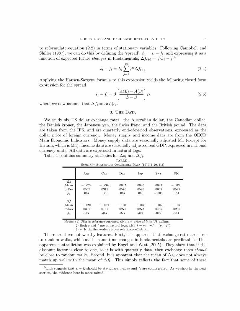
Table 1 contains summary statistics for ∆st and ∆ft.TABLE 1
Summary Statistics: Quarterly Data (1973:1-2011:3)
Aus Can Den Jap Swz UK
∆s
Mean −.0024 −.0002 .0007 .0080 .0083 −.0030
StDev .0547 .0311 .0576 .0590 .0649 .0529ρ1 .067 .178 .067 .060 −.008 .151
∆f
Mean −.0091 −.0071 −.0105 −.0035 −.0053 −.0136
StDev .0307 .0197 .0277 .0273 .0455 .0236ρ1 .197 .367 .277 .394 .092 .461
Notes: (1) USA is reference currency, with s = price of fx in US dollars.
(2) Both s and f are in natural logs, with f = m − m∗ − (y − y∗).(3) ρ1 is the first-order autocorrelation coefficient.
There are three noteworthy features. First, it is apparent that exchange rates are closeto random walks, while at the same time changes in fundamentals are predictable. Thisapparent contradiction was explained by Engel and West (2005). They show that if thediscount factor is close to one, as it is with quarterly data, then exchange rates should
be close to random walks. Second, it is apparent that the mean of ∆st does not alwaysmatch up well with the mean of ∆ft. This simply reflects the fact that some of these
5This suggests that st−ft should be stationary, i.e., st and ft are cointegrated. As we show in the nextsection, the evidence here is more mixed.
6 EDOUARD DJEUTEM AND KENNETH KASA
currencies have experienced long-run real appreciations or depreciations. This constitutesprima facie evidence against the monetary model, independent of its volatility implications.Our empirical work accounts for these missing trends by either detrending the data, orby including trends in posited cointegrating relationships. This gives the model the bestchance possible to explain exchange rate volatility. Third, and most importantly for thepurposes of our paper, note that the standard deviations of ∆st are around twice as largeas the standard deviations of ∆ft. Given the mild persistence in ∆ft, this is a majorproblem when it comes to explaining observed exchange rate volatility.
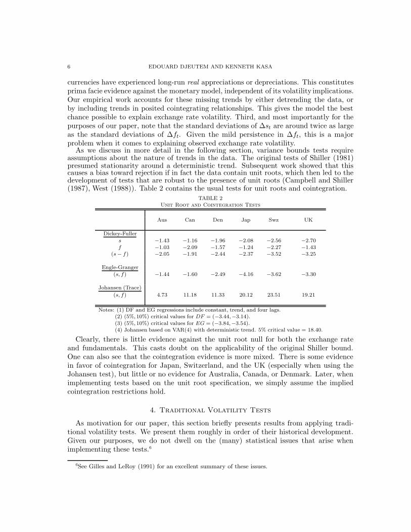
As we discuss in more detail in the following section, variance bounds tests requireassumptions about the nature of trends in the data. The original tests of Shiller (1981)presumed stationarity around a deterministic trend. Subsequent work showed that thiscauses a bias toward rejection if in fact the data contain unit roots, which then led to thedevelopment of tests that are robust to the presence of unit roots (Campbell and Shiller(1987), West (1988)). Table 2 contains the usual tests for unit roots and cointegration.
TABLE 2Unit Root and Cointegration Tests
Aus Can Den Jap Swz UK
Dickey-Fuller
s −1.43 −1.16 −1.96 −2.08 −2.56 −2.70
f −1.03 −2.09 −1.57 −1.24 −2.27 −1.43(s − f) −2.05 −1.91 −2.44 −2.37 −3.52 −3.25
Engle-Granger
(s, f) −1.44 −1.60 −2.49 −4.16 −3.62 −3.30
Johansen (Trace)
(s, f) 4.73 11.18 11.33 20.12 23.51 19.21
Notes: (1) DF and EG regressions include constant, trend, and four lags.(2) (5%,10%) critical values for DF = (−3.44,−3.14).
(3) (5%,10%) critical values for EG = (−3.84,−3.54).(4) Johansen based on VAR(4) with deterministic trend. 5% critical value = 18.40.
Clearly, there is little evidence against the unit root null for both the exchange rateand fundamentals. This casts doubt on the applicability of the original Shiller bound.One can also see that the cointegration evidence is more mixed. There is some evidencein favor of cointegration for Japan, Switzerland, and the UK (especially when using theJohansen test), but little or no evidence for Australia, Canada, or Denmark. Later, whenimplementing tests based on the unit root specification, we simply assume the impliedcointegration restrictions hold.
4. Traditional Volatility Tests
As motivation for our paper, this section briefly presents results from applying tradi-tional volatility tests. We present them roughly in order of their historical development.Given our purposes, we do not dwell on the (many) statistical issues that arise whenimplementing these tests.6
6See Gilles and LeRoy (1991) for an excellent summary of these issues.
ROBUSTNESS AND EXCHANGE RATE VOLATILITY 7
4.1. Shiller (1981). The attraction of Shiller’s original variance bound test is that it isbased on such a simple and compelling logic. Shiller noted that since asset prices arethe conditional expectation of the present value of future fundamentals, they should beless volatile than the ex post realized values of these fundamentals. More formally, if wedefine s∗t = (1− β)
∑∞j=0 β
jft+j as the ex post realized path of future fundamentals, thenthe monetary model is equivalent to the statement that st = Ets
∗t . Next, we can always
decompose a random variable into the sum of its conditional mean and an orthogonalforecast error,
s∗t = Ets∗t + ut
= st + ut
Since by construction the two terms on the right-hand side are orthogonal, we can takethe variance of both sides and get
σ2s∗ = σ2
s + σ2u ⇒ σ2
s ≤ σ2s∗
It’s as simple as that.7 Two practical issues arise when implementing the bound. First,prices and fundamentals clearly trend up over time. As a result, neither possesses a welldefined variance, so it is meaningless to apply the bounds test to the raw data. Shiller dealtwith this by linearly detrending the data. To maintain comparability, we do the same,although later we present results that are robust to the presence of unit roots. Second,future fundamentals are obviously unobserved beyond the end of the sample. Strictlyspeaking then, we cannot compute σ2
s∗ , and therefore, Shiller’s bound is untestable. Onecan always argue that agents within any given finite sample are acting on the basis ofsome as yet unobserved event. Of course, this kind of explanation is the last refugeof a scoundrel, and moreover, we show that it is unnecessary. Shiller handled the finitesample problem by assuming that s∗T , the end-of-sample forecast for the discounted presentvalue of future fundamentals, was simply given by the sample average. Unfortunately,subsequent researchers were quick to point out that this produces a bias toward rejection.So in this case, we depart from Shiller by using the unbiased procedure recommended byMankiw, Romer, and Shapiro (1985). This involves iterating on the backward recursions∗t = (1− β)ft + βs∗t+1, with the boundary condition, s∗T = sT .
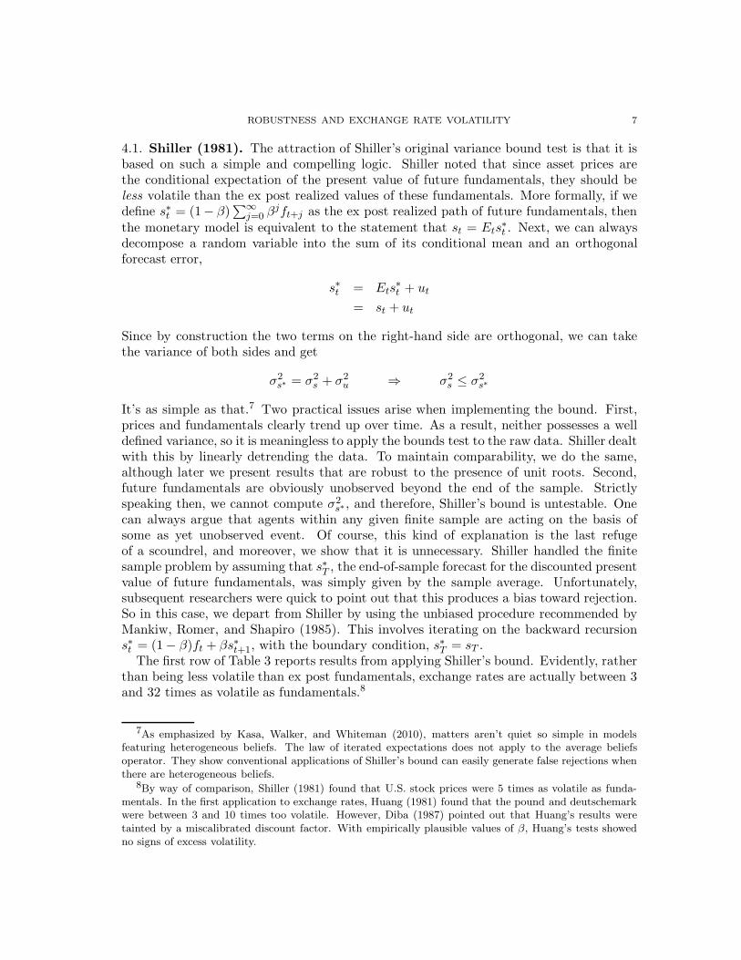
The first row of Table 3 reports results from applying Shiller’s bound. Evidently, ratherthan being less volatile than ex post fundamentals, exchange rates are actually between 3and 32 times as volatile as fundamentals.8
7As emphasized by Kasa, Walker, and Whiteman (2010), matters aren’t quiet so simple in modelsfeaturing heterogeneous beliefs. The law of iterated expectations does not apply to the average beliefsoperator. They show conventional applications of Shiller’s bound can easily generate false rejections whenthere are heterogeneous beliefs.
8By way of comparison, Shiller (1981) found that U.S. stock prices were 5 times as volatile as funda-mentals. In the first application to exchange rates, Huang (1981) found that the pound and deutschemarkwere between 3 and 10 times too volatile. However, Diba (1987) pointed out that Huang’s results weretainted by a miscalibrated discount factor. With empirically plausible values of β, Huang’s tests showedno signs of excess volatility.
8 EDOUARD DJEUTEM AND KENNETH KASA
TABLE 3Traditional Volatility Tests
Aus Can Den Jap Swz UK
Shillervar(s)/var(s∗) 3.13 7.85 25.7 2.93 14.2 32.5
Campbell-Shiller
var(φ)/var(φ∗) 3.41 10.2 7.98 211.2 178.2 9.00
West
var(ε)/var(ε) 2.36 1.81 2.33 1.34 1.73 1.77
Engel-West
var(∆s)/var(∆xH) 1.83 0.99 1.66 1.30 1.46 1.15
Engel
var(∆s)/var(∆s) 5.98 10.8 3.35 7.42 20.7 14.6
Notes: (1) Shiller bound based on detrended data, assuming s∗T = sT and β = .98.(2) Campbell-Shiller bound based on a VAR(2) for (∆f, φ), assuming β = .98.
(3) Engel-West bound based on AR(2) for ∆f , assuming β = .98 ≈ 1.(4) Engel bound based on AR(1) for detrended ft, assuming β = .98.
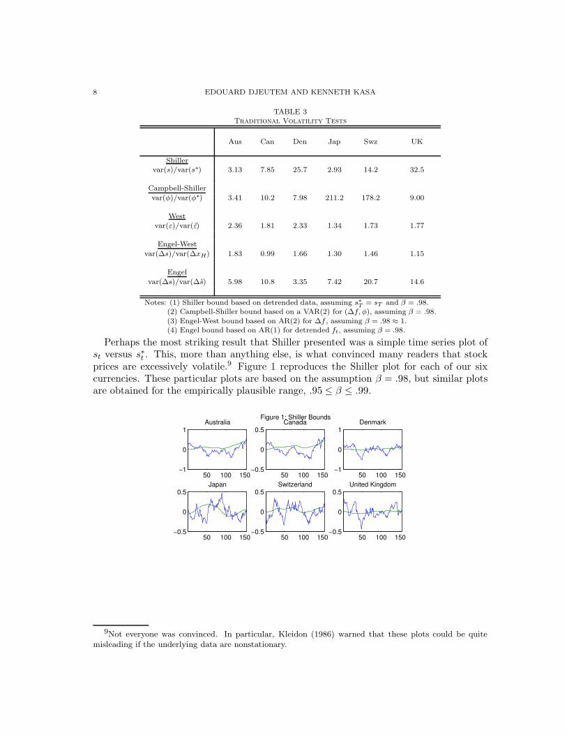
Perhaps the most striking result that Shiller presented was a simple time series plot ofst versus s∗t . This, more than anything else, is what convinced many readers that stockprices are excessively volatile.9 Figure 1 reproduces the Shiller plot for each of our sixcurrencies. These particular plots are based on the assumption β = .98, but similar plotsare obtained for the empirically plausible range, .95 ≤ β ≤ .99.
Figure 1: Shiller Bounds
50 100 150−1
0
1Australia
50 100 150−0.5
0
0.5Canada
50 100 150−1
0
1Denmark
50 100 150−0.5
0
0.5Japan
50 100 150−0.5
0
0.5Switzerland
50 100 150−0.5
0
0.5United Kingdom
9Not everyone was convinced. In particular, Kleidon (1986) warned that these plots could be quitemisleading if the underlying data are nonstationary.

ROBUSTNESS AND EXCHANGE RATE VOLATILITY 9
As with Shiller, these plots paint a clear picture of ‘excess volatility’. Unfortunately,there are enough statistical caveats and pitfalls associated with these results, that it isworthwhile to consider results from applying some of the more recently proposed boundstests, starting with the influential work of Campbell and Shiller (1987).
4.2. Campbell and Shiller (1987). The results of Shiller (1981) are sensitive to thepresence of unit roots in the data. As we saw in Table 2, there appear to be unit rootsin both st and ft (even after the removal of a deterministic trend). Campbell and Shiller(1987) devised a volatility test that is valid when the data are nonstationary. In addition,they devised a clever way of capturing potential information that market participantsmight have about future fundamentals that is unobserved by outside econometricians. Todo this, one simply needs to include current and lagged values of the exchange rate whenforecasting future fundamentals. Under the null, the current exchange rate is a sufficientstatistic for the present value of future fundamentals. Forecasting future fundamentalswith a VAR that includes the exchange rate converts Shiller’s variance bound inequalityto a variance equality. The model-implied forecast of the present value of fundamentalsshould be identically equal to the actual exchange rate!
To handle unit roots, Campbell and Shiller (1987) presume that st and ft are cointe-grated, and then define the ‘spread’ variable φt = st − ft. The model implies that φt isthe expected present value of future values of ∆ft (see eq. (2.4)). If we define the vector(∆ft, φt)
′ we can then estimate the following VAR,
xt = Ψ(L)xt−1 + εt
By adding lags to the state, this can always be expressed as a VAR(1)
xt = Ψxt−1 + εt
where Ψ is a double companion matrix, and the first element of xt is ∆ft. The model-implied spread, φ∗t , is given by the expected present discounted value of {∆ft+j}, whichcan be expressed in terms of observables as follows,
φ∗t = e1′βΨ(I − βΨ)−1xt (4.6)
where e1 is a selection vector that picks off the first element of xt. The model thereforeimplies var(φt) = var(φ∗t ).
The second row of Table 3 reports values of var(φt)/var(φ∗t ) based on a VAR(2) model(including a trend and intercept). We fix β = .98, although the results are similar forvalues in the range .95 ≤ β ≤ .99. Although Campbell and Shiller’s approach is quitedifferent, the results are quite similar. All ratios substantially exceed unity. Although theCampbell-Shiller method points to relatively less volatility in Denmark and the UK, itactually suggests greater excess volatility for Japan and Switzerland.
4.3. West (1988). West (1988) proposed an alternative test that is also robust to thepresence of unit roots. Rather than look directly at the volatility of observed prices andfundamentals, West’s test is based on comparison of two innovation variances. Theseinnovations can be interpreted as one-period holding returns, and so are stationary evenwhen the underlying price and fundamentals processes are nonstationary. Following West(1988), let It be the market information set at time-t, and let Ht ⊆ It be some subset
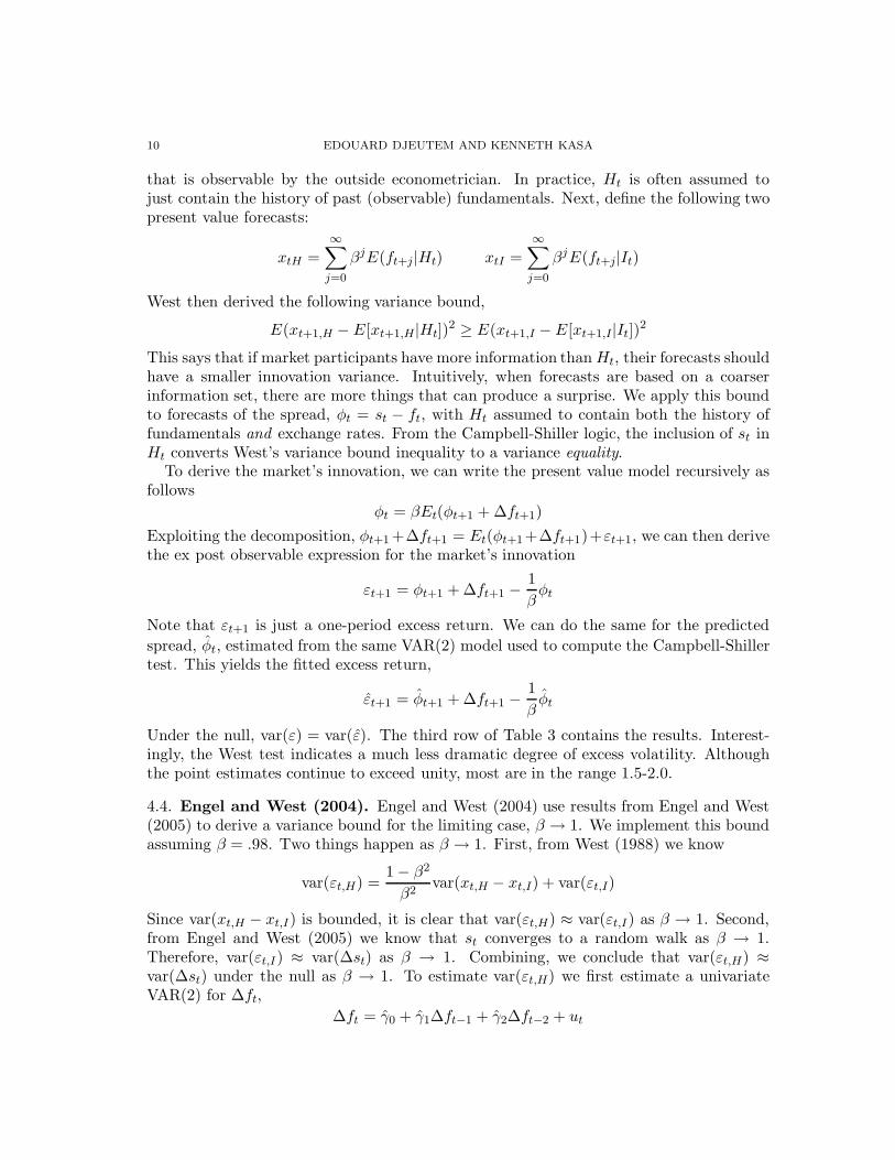
10 EDOUARD DJEUTEM AND KENNETH KASA
that is observable by the outside econometrician. In practice, Ht is often assumed tojust contain the history of past (observable) fundamentals. Next, define the following twopresent value forecasts:
xtH =
∞∑
j=0
βjE(ft+j|Ht) xtI =
∞∑
j=0
βjE(ft+j|It)
West then derived the following variance bound,
E(xt+1,H − E[xt+1,H|Ht])2 ≥ E(xt+1,I − E[xt+1,I|It])2
This says that if market participants have more information thanHt, their forecasts shouldhave a smaller innovation variance. Intuitively, when forecasts are based on a coarserinformation set, there are more things that can produce a surprise. We apply this boundto forecasts of the spread, φt = st − ft, with Ht assumed to contain both the history offundamentals and exchange rates. From the Campbell-Shiller logic, the inclusion of st inHt converts West’s variance bound inequality to a variance equality.
To derive the market’s innovation, we can write the present value model recursively asfollows
φt = βEt(φt+1 + ∆ft+1)
Exploiting the decomposition, φt+1 +∆ft+1 = Et(φt+1+∆ft+1)+εt+1, we can then derivethe ex post observable expression for the market’s innovation
εt+1 = φt+1 + ∆ft+1 −1
βφt
Note that εt+1 is just a one-period excess return. We can do the same for the predicted
spread, φt, estimated from the same VAR(2) model used to compute the Campbell-Shillertest. This yields the fitted excess return,
εt+1 = φt+1 + ∆ft+1 −1
βφt
Under the null, var(ε) = var(ε). The third row of Table 3 contains the results. Interest-ingly, the West test indicates a much less dramatic degree of excess volatility. Althoughthe point estimates continue to exceed unity, most are in the range 1.5-2.0.
4.4. Engel and West (2004). Engel and West (2004) use results from Engel and West(2005) to derive a variance bound for the limiting case, β → 1. We implement this boundassuming β = .98. Two things happen as β → 1. First, from West (1988) we know
var(εt,H) =1 − β2
β2var(xt,H − xt,I) + var(εt,I)
Since var(xt,H − xt,I) is bounded, it is clear that var(εt,H) ≈ var(εt,I) as β → 1. Second,from Engel and West (2005) we know that st converges to a random walk as β → 1.Therefore, var(εt,I) ≈ var(∆st) as β → 1. Combining, we conclude that var(εt,H) ≈var(∆st) under the null as β → 1. To estimate var(εt,H) we first estimate a univariateVAR(2) for ∆ft,
∆ft = γ0 + γ1∆ft−1 + γ2∆ft−2 + ut

ROBUSTNESS AND EXCHANGE RATE VOLATILITY 11
We can then estimate var(εt,H) as follows
var(εt,H) = (1− βγ1 − β2γ2)−2var(u)
The fourth row of Table 3 reports the ratio var(∆st)/var(εt,H) for each of our six currencies.Overall, the results are quite similar to the results from the West test, the only significantdifference being Canada, which has a point estimate (slightly) below unity. The results arealso quite similar to those reported by Engel and West (2004), although as noted earlier,they interpret the results reciprocally, as the share of exchange rate volatility that can beaccounted for by observed fundamentals.
4.5. Engel (2005). Engel (2005) derives a variance bound that is closely related to theWest (1988) bound. Like the West bound, it is robust to the presence of unit roots. Let stbe the forecast of the present discounted value of future fundamentals based on a subset,Ht, of the market’s information. Engel shows that the model, along with the RationalExpectations Hypothesis, implies the following inequality10
var(st − st−1) ≤ var(st − st−1)
For simplicity, we test this bound by assuming that ft follows an AR(1) around a de-
terministic trend. That is, letting ft denote the demeaned and detrended ft process, weassume ft = ρft−1 + ut. In this case, we have
st = α0 + α1 · t+
(
1 − β
1 − ρβ
)
ft ⇒ ∆st =
(
1 − β
1 − ρβ
)
∆ft
The bottom row reports values of var(∆st)/var(∆st). Not surprisingly, given our previ-ous results, they all exceed unity by a substantial margin, once again pointing to excessvolatility in the foreign exchange market.
5. Robust Volatility Tests
The results reported in the previous section are based on tests that make different as-sumptions about information, trends, and the underlying data generating process. Despitethis, a consistent picture emerges - exchange rates appear to exhibit ‘excess volatility’. Ofcourse, we haven’t reported standard errors, so it is possible these results lack statisticalsignificance (although we doubt it). However, we agree with Shiller (1989). Pinning yourhopes on a lack of significance does not really provide much support for the model. Itmerely says there isn’t enough evidence yet to reject it.
Although the previous tests differ along several dimensions, there is one assumptionthey all share, namely, the Rational Expectations Hypothesis (REH). As noted earlier,this is a joint hypothesis, based on two assumptions: (1) Agents have common knowl-edge of the correct model, and (2) Agents make statistically optimal forecasts. Of course,many previous researchers have interpreted Shiller’s work as evidence against the Ratio-nal Expectations Hypothesis (including Shiller himself!). However, there is an important
10Engel (2005) also derives a second bound. As before, let s∗t denote the ex post realized present valueof future fundamentals. Engel shows that the model implies var(s∗t − s∗t−1) ≤ var(st − st−1). Note, this islike the Shiller bound, but in first differences. However, note that the direction of the bound is reversed!Although we haven’t formally checked it, given our previous results, we suspect this bound would be easilysatisfied.
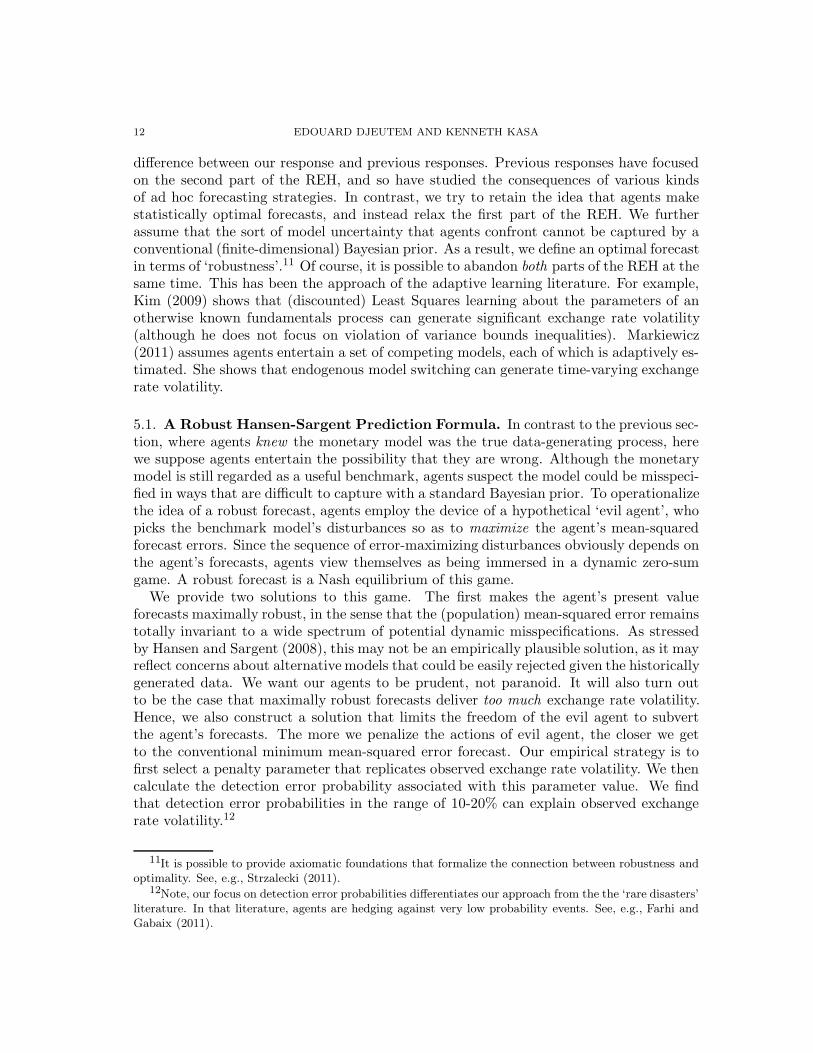
12 EDOUARD DJEUTEM AND KENNETH KASA
difference between our response and previous responses. Previous responses have focusedon the second part of the REH, and so have studied the consequences of various kindsof ad hoc forecasting strategies. In contrast, we try to retain the idea that agents makestatistically optimal forecasts, and instead relax the first part of the REH. We furtherassume that the sort of model uncertainty that agents confront cannot be captured by aconventional (finite-dimensional) Bayesian prior. As a result, we define an optimal forecastin terms of ‘robustness’.11 Of course, it is possible to abandon both parts of the REH at thesame time. This has been the approach of the adaptive learning literature. For example,Kim (2009) shows that (discounted) Least Squares learning about the parameters of anotherwise known fundamentals process can generate significant exchange rate volatility(although he does not focus on violation of variance bounds inequalities). Markiewicz(2011) assumes agents entertain a set of competing models, each of which is adaptively es-timated. She shows that endogenous model switching can generate time-varying exchangerate volatility.
5.1. A Robust Hansen-Sargent Prediction Formula. In contrast to the previous sec-tion, where agents knew the monetary model was the true data-generating process, herewe suppose agents entertain the possibility that they are wrong. Although the monetarymodel is still regarded as a useful benchmark, agents suspect the model could be misspeci-fied in ways that are difficult to capture with a standard Bayesian prior. To operationalizethe idea of a robust forecast, agents employ the device of a hypothetical ‘evil agent’, whopicks the benchmark model’s disturbances so as to maximize the agent’s mean-squaredforecast errors. Since the sequence of error-maximizing disturbances obviously depends onthe agent’s forecasts, agents view themselves as being immersed in a dynamic zero-sumgame. A robust forecast is a Nash equilibrium of this game.
We provide two solutions to this game. The first makes the agent’s present valueforecasts maximally robust, in the sense that the (population) mean-squared error remainstotally invariant to a wide spectrum of potential dynamic misspecifications. As stressedby Hansen and Sargent (2008), this may not be an empirically plausible solution, as it mayreflect concerns about alternative models that could be easily rejected given the historicallygenerated data. We want our agents to be prudent, not paranoid. It will also turn outto be the case that maximally robust forecasts deliver too much exchange rate volatility.Hence, we also construct a solution that limits the freedom of the evil agent to subvertthe agent’s forecasts. The more we penalize the actions of evil agent, the closer we getto the conventional minimum mean-squared error forecast. Our empirical strategy is tofirst select a penalty parameter that replicates observed exchange rate volatility. We thencalculate the detection error probability associated with this parameter value. We findthat detection error probabilities in the range of 10-20% can explain observed exchangerate volatility.12
11It is possible to provide axiomatic foundations that formalize the connection between robustness andoptimality. See, e.g., Strzalecki (2011).
12Note, our focus on detection error probabilities differentiates our approach from the the ‘rare disasters’literature. In that literature, agents are hedging against very low probability events. See, e.g., Farhi andGabaix (2011).
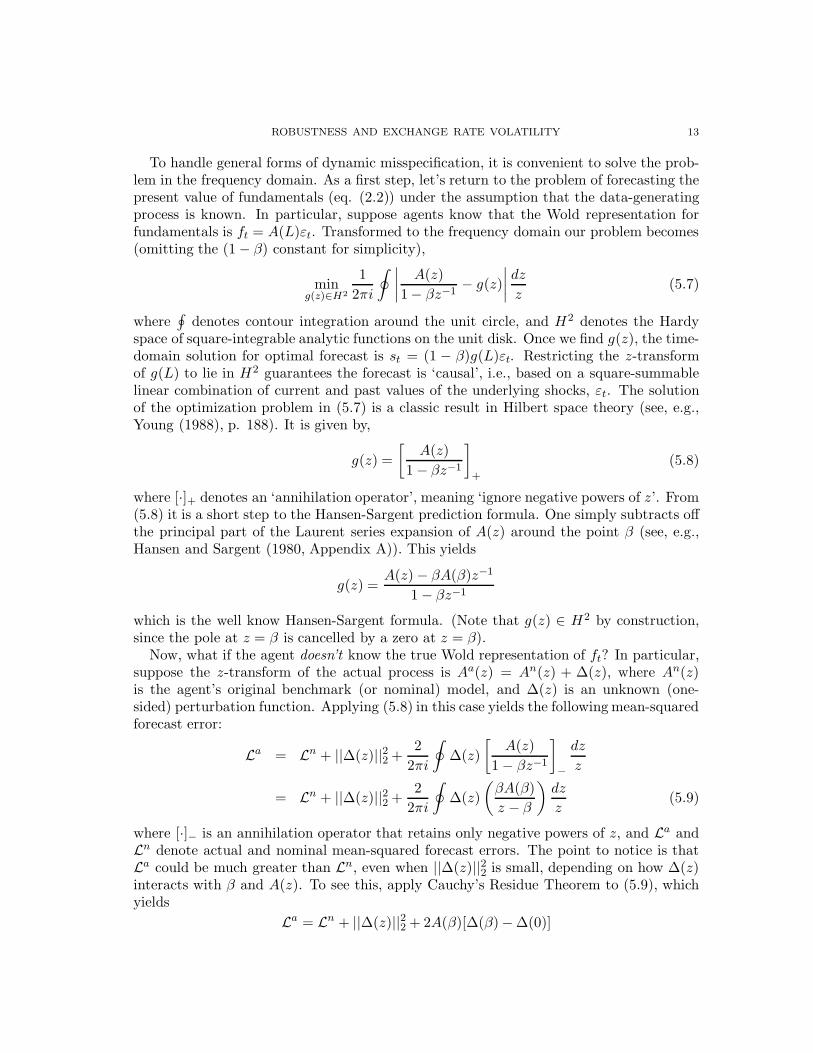
ROBUSTNESS AND EXCHANGE RATE VOLATILITY 13
To handle general forms of dynamic misspecification, it is convenient to solve the prob-lem in the frequency domain. As a first step, let’s return to the problem of forecasting thepresent value of fundamentals (eq. (2.2)) under the assumption that the data-generatingprocess is known. In particular, suppose agents know that the Wold representation forfundamentals is ft = A(L)εt. Transformed to the frequency domain our problem becomes(omitting the (1 − β) constant for simplicity),
ming(z)∈H2
1
2πi
∮
∣
∣
∣
∣
A(z)
1− βz−1− g(z)
∣
∣
∣
∣
dz
z(5.7)
where∮
denotes contour integration around the unit circle, and H2 denotes the Hardyspace of square-integrable analytic functions on the unit disk. Once we find g(z), the time-domain solution for optimal forecast is st = (1 − β)g(L)εt. Restricting the z-transformof g(L) to lie in H2 guarantees the forecast is ‘causal’, i.e., based on a square-summablelinear combination of current and past values of the underlying shocks, εt. The solutionof the optimization problem in (5.7) is a classic result in Hilbert space theory (see, e.g.,Young (1988), p. 188). It is given by,
g(z) =
[
A(z)
1 − βz−1
]
+
(5.8)
where [·]+ denotes an ‘annihilation operator’, meaning ‘ignore negative powers of z’. From(5.8) it is a short step to the Hansen-Sargent prediction formula. One simply subtracts offthe principal part of the Laurent series expansion of A(z) around the point β (see, e.g.,Hansen and Sargent (1980, Appendix A)). This yields
g(z) =A(z) − βA(β)z−1
1 − βz−1
which is the well know Hansen-Sargent formula. (Note that g(z) ∈ H2 by construction,since the pole at z = β is cancelled by a zero at z = β).
Now, what if the agent doesn’t know the true Wold representation of ft? In particular,suppose the z-transform of the actual process is Aa(z) = An(z) + ∆(z), where An(z)is the agent’s original benchmark (or nominal) model, and ∆(z) is an unknown (one-sided) perturbation function. Applying (5.8) in this case yields the following mean-squaredforecast error:
La = Ln + ||∆(z)||22 +2
2πi
∮
∆(z)
[
A(z)
1 − βz−1
]
−
dz
z
= Ln + ||∆(z)||22 +2
2πi
∮
∆(z)
(
βA(β)
z − β
)
dz
z(5.9)
where [·]− is an annihilation operator that retains only negative powers of z, and La andLn denote actual and nominal mean-squared forecast errors. The point to notice is thatLa could be much greater than Ln, even when ||∆(z)||22 is small, depending on how ∆(z)interacts with β and A(z). To see this, apply Cauchy’s Residue Theorem to (5.9), whichyields
La = Ln + ||∆(z)||22 + 2A(β)[∆(β)− ∆(0)]
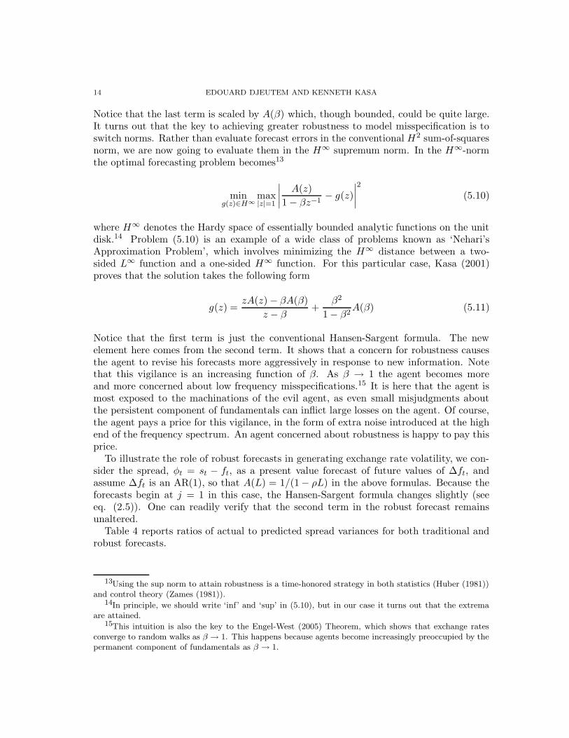
14 EDOUARD DJEUTEM AND KENNETH KASA
Notice that the last term is scaled by A(β) which, though bounded, could be quite large.It turns out that the key to achieving greater robustness to model misspecification is toswitch norms. Rather than evaluate forecast errors in the conventional H2 sum-of-squaresnorm, we are now going to evaluate them in the H∞ supremum norm. In the H∞-normthe optimal forecasting problem becomes13
ming(z)∈H∞
max|z|=1
∣
∣
∣
∣
A(z)
1 − βz−1− g(z)
∣
∣
∣
∣
2
(5.10)
where H∞ denotes the Hardy space of essentially bounded analytic functions on the unitdisk.14 Problem (5.10) is an example of a wide class of problems known as ‘Nehari’sApproximation Problem’, which involves minimizing the H∞ distance between a two-sided L∞ function and a one-sided H∞ function. For this particular case, Kasa (2001)proves that the solution takes the following form
g(z) =zA(z) − βA(β)
z − β+
β2
1− β2A(β) (5.11)
Notice that the first term is just the conventional Hansen-Sargent formula. The newelement here comes from the second term. It shows that a concern for robustness causesthe agent to revise his forecasts more aggressively in response to new information. Notethat this vigilance is an increasing function of β. As β → 1 the agent becomes moreand more concerned about low frequency misspecifications.15 It is here that the agent ismost exposed to the machinations of the evil agent, as even small misjudgments aboutthe persistent component of fundamentals can inflict large losses on the agent. Of course,the agent pays a price for this vigilance, in the form of extra noise introduced at the highend of the frequency spectrum. An agent concerned about robustness is happy to pay thisprice.
To illustrate the role of robust forecasts in generating exchange rate volatility, we con-sider the spread, φt = st − ft, as a present value forecast of future values of ∆ft, andassume ∆ft is an AR(1), so that A(L) = 1/(1− ρL) in the above formulas. Because theforecasts begin at j = 1 in this case, the Hansen-Sargent formula changes slightly (seeeq. (2.5)). One can readily verify that the second term in the robust forecast remainsunaltered.
Table 4 reports ratios of actual to predicted spread variances for both traditional androbust forecasts.
13Using the sup norm to attain robustness is a time-honored strategy in both statistics (Huber (1981))and control theory (Zames (1981)).
14In principle, we should write ‘inf’ and ‘sup’ in (5.10), but in our case it turns out that the extremaare attained.
15This intuition is also the key to the Engel-West (2005) Theorem, which shows that exchange ratesconverge to random walks as β → 1. This happens because agents become increasingly preoccupied by thepermanent component of fundamentals as β → 1.
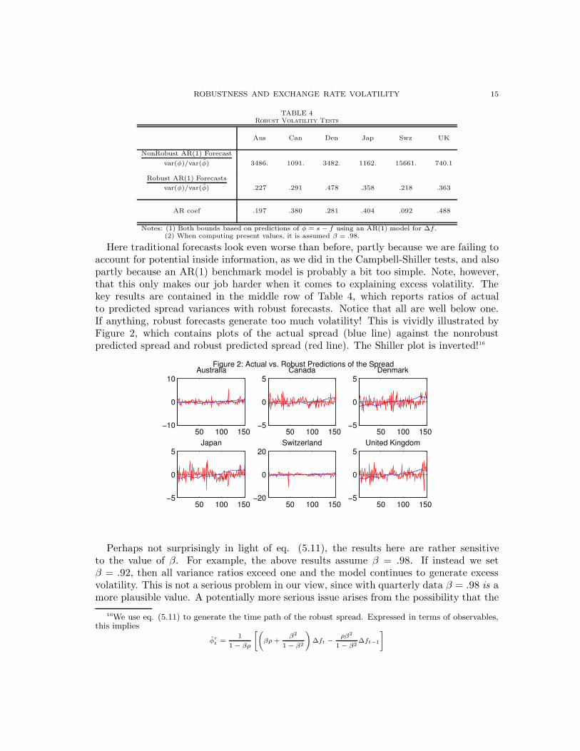
ROBUSTNESS AND EXCHANGE RATE VOLATILITY 15
TABLE 4Robust Volatility Tests
Aus Can Den Jap Swz UK
NonRobust AR(1) Forecast
var(φ)/var(φ) 3486. 1091. 3482. 1162. 15661. 740.1
Robust AR(1) Forecasts
var(φ)/var(φ) .227 .291 .478 .358 .218 .363
AR coef .197 .380 .281 .404 .092 .488
Notes: (1) Both bounds based on predictions of φ = s − f using an AR(1) model for ∆f.(2) When computing present values, it is assumed β = .98.
Here traditional forecasts look even worse than before, partly because we are failing toaccount for potential inside information, as we did in the Campbell-Shiller tests, and alsopartly because an AR(1) benchmark model is probably a bit too simple. Note, however,that this only makes our job harder when it comes to explaining excess volatility. Thekey results are contained in the middle row of Table 4, which reports ratios of actualto predicted spread variances with robust forecasts. Notice that all are well below one.If anything, robust forecasts generate too much volatility! This is vividly illustrated byFigure 2, which contains plots of the actual spread (blue line) against the nonrobustpredicted spread and robust predicted spread (red line). The Shiller plot is inverted!16
Figure 2: Actual vs. Robust Predictions of the Spread
50 100 150−10
0
10Australia
50 100 150−5
0
5Canada
50 100 150−5
0
5Denmark
50 100 150−5
0
5Japan
50 100 150−20
0
20Switzerland
50 100 150−5
0
5United Kingdom
Perhaps not surprisingly in light of eq. (5.11), the results here are rather sensitiveto the value of β. For example, the above results assume β = .98. If instead we setβ = .92, then all variance ratios exceed one and the model continues to generate excessvolatility. This is not a serious problem in our view, since with quarterly data β = .98 is amore plausible value. A potentially more serious issue arises from the possibility that the
16We use eq. (5.11) to generate the time path of the robust spread. Expressed in terms of observables,this implies
φr
t=
1
1 − βρ
"
βρ +β2
1 − β2
!
∆ft −
ρβ2
1 − β2∆ft−1
#

16 EDOUARD DJEUTEM AND KENNETH KASA
agent is being excessively pessimistic here, and is worrying about alternative models thathave little likelihood of being the true data-generating process. Fortunately, it is easy toavoid this problem by parameterizing the agent’s concern for robustness. We do this bypenalizing the actions of the evil agent.
5.2. The Evil Agent Game. The previous results incorporated robustness by evaluatingforecast errors in the H∞-norm. This delivers the maximal degree of robustness, butmay entail unduly pessimistic beliefs. Following Lewis and Whiteman (2008), we nowgo back to the H2-norm, and instead model robustness by penalizing the actions of thehypothetical evil agent. In particular, we assume the evil agent picks shocks subject to aquadratic penalty. As emphasized by Hansen and Sargent (2008), a quadratic penalty isconvenient, since in Gaussian environments it can be related to entropy distortions andthe Kullback-Leibler Information Criterion, which then opens to door to an interpretationof the agent’s worst-case model in terms of detection error probabilities. This allows us toplace empirically plausible bounds on the evil agent’s actions.
Since our methods presume stationarity, we assume the agent has a benchmark (nom-inal) model, ∆ft = An(L)εt. In the conventional monetary model, this determines thespread, φt = st − ft, as in (2.4). At the same time, he realizes this model may be sub-ject to unstructured perturbations of the form ∆(L)εt, so that the actual model becomes,∆ft = Aa(L)εt = An(L)εt + ∆(L)εt. The Evil Agent Game involves the agent selectinga forecast function, g(L), to minimize mean-squared forecast errors, while at the sametime the evil agent picks the distortion function, ∆(L). Hence, both agents must solve acalculus of variations problem. These problems are related to each other, and so we mustsolve for a Nash equilibrium. Following Lewis and Whiteman (2008), we can express theproblem in the frequency domain as follows
ming(z)
maxAa(z)
1
2πi
∮
{
∣
∣
∣
∣
βz−1Aa(z)
1− βz−1− g(z)
∣
∣
∣
∣
2
− θ
∣
∣
∣
∣
Aa(z)− An(z)
1 − βz−1
∣
∣
∣
∣
2}
dz
z(5.12)
where for convenience we assume the evil agent picks Aa(z) rather than ∆(z). The keyelement here is the parameter θ. It penalizes the actions of the evil agent. By increasingθ we get closer to the conventional minimum mean-squared error forecast. Conversely,the smallest value of θ that is consistent with the concavity of the evil agent’s problemdelivers the maximally robust H∞ solution.
The Wiener-Hopf first-order condition for the agent’s problem is
g(z)− βz−1
1 − βz−1Aa(z) =
−1∑
∞
(5.13)
where∑−1
∞ denotes an arbitrary function in negative powers of z. The evil agent’s Wiener-Hopf equation can be written
(β2 − θ)Aa(z)
1 − βz− βz
1 − βz−1
1 − βzg(z) +
θAn(z)
1 − βz=
−1∑
∞
(5.14)
ROBUSTNESS AND EXCHANGE RATE VOLATILITY 17
Applying the annihilation operator to both sides of eq. (5.13), we can then solve for theagent’s policy in terms of the policy of the evil agent
g(z) = βAa(z) −Aa(β)
z − β
Then, if we substitute this into the evil agent’s first-order condition and apply the anni-hilation operator we get
(β2 − θ)Aa(z)
1 − βz− β2A
a(z) − Aa(β)
1 − βz+θAn(z)
1 − βz= 0
which then implies
Aa(z) = An(z) +β2
θAa(β) (5.15)
To determine Aa(β) we can evaluate the evil agent’s first-order condition (5.14) at z = β,
which implies Aa(β) =θAn(β)θ−β2 . Substituting this back into (5.15) yields
Aa(z) = An(z) +β2
θ − β2An(β) (5.16)
This gives the worst-case model associated with any given benchmark model. In game-theoretic terms, it represents the evil agent’s reaction function. Notice that as θ → ∞ werecover the conventional minimum mean-squared error solution. Conversely, notice theclose correspondence to the previous H∞ solution when θ = 1.
5.3. Detection Error Calibration. The idea here is that the agent believes An(L)εtis a useful first-approximation to the actual data-generating process. However, he alsorecognizes that if he is wrong, he could suffer large losses. To minimize his exposure tothese losses, he acts as if ∆ft = Aa(L)εt is the data-generating process when formulatinghis present value forecasts. Reducing θ makes his forecasts more robust, but producesunnecessary noise if in fact the benchmark model is correct. To gauge whether observedexchange rate volatility might simply reflect a reasonable response to model uncertainty,we now ask the following question - Suppose we calibrate θ to match the observed volatilityof the spread, st −ft. (We know this is possible from the H∞ results). Given this impliedvalue of θ, how easy would it be for the agent to statistically distinguish the worst-casemodel, Aa(L), from the benchmark monetary model, An(L)? If the two would be easy todistinguish, then our explanation doesn’t carry much force. However, if the probabilityof a detection error is reasonably large, then we claim that model uncertainty provides areasonable explanation of observed exchange rate volatility.
To begin, we need to take a stand on the benchmark model. For simplicity, we assume∆ft follows an AR(1), so that An(L) = 1/(1 − ρL). (We de-mean the data). Given this,note that eq. (5.16) then implies the worst case model, Aa(L), is an ARMA(1,1), withthe same AR root. To facilitate notation, we write this model as follows,
∆ft =1 + κ− ρκL
1 − ρLεt
where κ ≡ β2
θ−β2
11−ρβ . Notice that κ → 0 as θ → ∞, and the two models become increas-
ingly difficult to distinguish. As always, there are two kinds of inferential errors the agent

18 EDOUARD DJEUTEM AND KENNETH KASA
could make: (1) He could believe An is the true model, when in fact Aa is the true model,or (2) He could believe Aa is the true model, when in fact An is the true model. Denotethe probability of the first error by P (An|Aa), and the probability of the second errorby P (Aa|An). Following Hansen and Sargent (2008), we treat the two errors symmetri-cally, and define the detection error probability, E , to be 1
2 [P (An|Aa) + P (Aa|An)]. FromTaniguchi and Kakizawa (2000) (pgs. 500-503), we have the following frequency domainapproximation to this detection error probability,
E =1
2
{
Φ
[
−√TI(An, Aa)
V (An, Aa)
]
+ Φ
[
−√TI(Aa, An)
V (Aa, An)
]}
(5.17)
where T is the sample size and Φ denotes the Gaussian cdf.17 Note that detection errorprobabilities decrease with T . The I functions in (5.17) are the KLIC ‘distances’ betweenthe two models, given by
I(An, Aa) =1
4π
∫ π
−π
[
− log|An(ω)||Aa(ω)| +
An(ω)
Aa(ω)− 1
]
dω (5.18)
I(Aa, An) =1
4π
∫ π
−π
[
− log|Aa(ω)||An(ω)| +
Aa(ω)
An(ω)− 1
]
dω (5.19)
The V functions in (5.17) can be interpreted as standard errors. They are given by thesquare roots of the following variance functions
V 2(An, Aa) =1
4π
∫ π
−π
[
An(ω)
(
1
An(ω)− 1
Aa(ω)
)]2
dω (5.20)
V 2(Aa, An) =1
4π
∫ π
−π
[
Aa(ω)
(
1
Aa(ω)− 1
An(ω)
)]2
dω (5.21)
By substituting in the expressions for Aa and An and performing the integrations, weobtain the following expressions for I functions18
I(An, Aa) =1
2
[
log(1 + κ) +1
(1 + κ)2(1 − ψ2)− 1
]
I(Aa, An) =1
2
[
− log(1 + κ) + (1 + κ)2(1 + ψ2) − 1]
17The same formula applies even when the underlying data are non-Gaussian. All that changes is thathigher-order cumulants must be added to the variance terms in (5.20)-(5.21). However, for simplicity, wesuppose the agent knows the data are Gaussian. Intuitively, we suspect that relaxing this assumptionwould only strengthen our results.
18We employed the following trick when evaluating these integrals. First, if An(L) = 1
1−ρL, we can then
write Aa = (1+κ) 1−ψL
1−ρL, where κ is defined above and ψ = ρκ/(1+κ). We then have (omitting inessential
constants)I
− log|An|
|Aa|
dz
z=
I
log(1 + κ)dz
z+
I
log
˛
˛
˛
˛
1− ψz
1 − ρz
˛
˛
˛
˛
dz
z−
I
log
˛
˛
˛
˛
1
1− ρz
˛
˛
˛
˛
dz
z= log(1 + κ)
where the last equality follows from the well known innovation formula, 1
2π
R π
−πlog f(ω)dω = log(σ2),
where f(ω) is the spectral density of a process, and σ2 is its innovation variance. This cancels the last twoterms since they have the same innovation variance. The same trick can be used to evaluate the other logintegral.

ROBUSTNESS AND EXCHANGE RATE VOLATILITY 19
where ψ ≡ ρκ/(1 + κ). As a simple reality check, note that θ → ∞ ⇒ κ → 0 ⇒ I → 0,which we know must be the case. Now, doing the same thing for the V functions gives us
V 2(An, Aa) =1
2
1
(1 + κ)2(1− ψ2)
[
(1 + κ)4 − 2(1 + κ)2 +1 + ψ2
(1 − ψ2)2
]
V 2(Aa, An) =1
2
[
1
(1 + κ)2− 2(1 + ψ2) + (1 + 4ψ2 + ψ4)(1 + κ)2
]
We use these formulas as follows. First, we estimate country-specific values of ρ. Theseare given in the bottom row of Table 4. Then we calibrate θ for each country to match theobserved variance of its spread, st−ft. The resulting values are reported in the first row ofTable 5. Since the earlier H∞ forecasts generated too much volatility, it is not surprisingthat the implied values of θ all exceed one (but not by much). Finally, as we have donethroughout, we set β = .98. We can then calculate the κ and ψ parameters that appearin the above detection error formulas. The results are contained in the second and thirdrows of Table 5.
TABLE 5
Evil Agent Game: Calibrated Detection Errors
Aus Can Den Jap Swz UK
θ 1.0442 1.0349 1.0178 1.0273 1.0454 1.0220
Det Error Prob(T = 150) .083 .109 .112 .119 .075 .131
Det Error Prob (T = 100) .107 .131 .134 .140 .099 .151
Notes: (1) θ calibrated to match observed variance of φ = s − f .
(2) When computing present values, it is assumed β = .98.
We report detection error probabilities for two different sample sizes. The first assumesT = 150, which is (approximately) the total number of quarterly observations availablein our post-Bretton Woods sample. In this case, the agent could distinguish the twomodels at approximately the 10% significance level.19 Although one could argue thisentails excessive pessimism, keep in mind that the data are generated in real-time, and soagents did not have access to the full sample when the data were actually being generated.As an informal correction for this, we also report detection error probabilities assumingT = 100. Now the detection error probabilities lie between 10-15%.
6. Concluding Remarks
This paper has proposed a solution to the excess volatility puzzle in foreign exchangemarkets. Our solution is based on a disciplined retreat from the Rational ExpectationsHypothesis. We abandon the assumption that agents know the correct model of the
19It is a little misleading to describe these results in the language of hypothesis testing. The agent is notconducting a traditional hypothesis test, since both models are treated symmetrically. It is more accurateto think of the agent as conducting a pair of hypothesis tests with two different nulls, or even better, asa Bayesian who is selecting between models with a uniform prior. The detection error probability is thenexpected loss under a 0-1 loss function.
20 EDOUARD DJEUTEM AND KENNETH KASA
economy, while retaining a revised notion of statistically optimal forecasts. We showthat an empirically plausible concern for robustness can explain observed exchange ratevolatility, even in a relatively simple environment like the constant discount rate/flexible-price monetary model.
Of course, there are many competing explanations already out there, so why is oursbetter? We think our approach represents a nice compromise between the two usual routestaken toward explaining exchange rate volatility. One obvious way to generate volatilityis to assume the existence of bubbles, herds, or sunspots. Although these models retainthe idea that agents make rational (self-fulfilling) forecasts, in our opinion they rely on animplausible degree of expectation coordination. Moreover, they are often not robust tominor changes in market structure or information. At the other end of the spectrum, manyso-called ‘behavioral’ explanations have the virtue of not relying on strong coordinationassumptions, but only resolve the puzzle by introducing rather drastic departures fromconventional notions of optimality.
As noted at the outset, our paper is closely related to Lewis and Whiteman (2008). Theyargue that robustness can explain observed US stock market volatility. However, they alsofind that if detection errors are based only on the agent’s ability to discriminate betweenalternative models for the economy’s exogenous dividend process, then implausibly smalldetection error probabilities are required. If instead detection errors are based on theagent’s ability to discriminate between bivariate models of dividends and prices, then stockmarket volatility can be accounted for with reasonable detection errors. This is not at allsurprising, since robustness delivers a substantially improved fit for prices. Interestingly,we find that even if detection errors are only based on the exogenous fundamentals process,exchange rate volatility can be accounted for with reasonable detection error probabilities.Still, one could argue that they are a bit on the low side, so it might be a useful extension toapply the bivariate Lewis-Whiteman approach to computing detection error probabilities.We conjecture that this would only strengthen our results.

ROBUSTNESS AND EXCHANGE RATE VOLATILITY 21
References
Arifovic, J. (1996): “The Behavior of the Exchange Rate in the Genetic Algorithm and ExperimentalEconomies,” Journal of Political Economy, 104, 510–41.
Campbell, J. Y., and R. J. Shiller (1987): “Cointegration and Tests of Present Value Models,” Journal
of Political Economy, 95, 1062–1088.Colacito, R., and M. M. Croce (2011): “International Asset Pricing with Risk-Sensitive Agents,”mimeo, University of North Carolina.
Diba, B. T. (1987): “A Critique of Variance Bounds Tests for Monetary Exchange Rate Models,” Journal
of Money, Credit and Banking, 19, 104–111.Engel, C. (2005): “Some New Variance Bounds for Asset Prices,” Journal of Money, Credit and Banking,37, 949–955.
Engel, C., N. Mark, and K. D. West (2007): “Exchange Rate Models Are Not As Bad As You Think,”NBER Macroeconomics Annual, 22, 381–441.
Engel, C., and K. D. West (2004): “Accounting for Exchange Rate Variability in Present-Value ModelsWhen the Discount Factor is Near 1,” American Economic Review, 94, 119–125.
(2005): “Exchange Rates and Fundamentals,” Journal of Political Economy, 113(3), 485–517.Evans, G. W. (1986): “A Test for Speculative Bubbles in the Sterling-Dollar Exchange Rate: 1981-84,”American Economic Review, 76, 621–36.
Farhi, E., and X. Gabaix (2011): “Rare Disasters and Exchange Rates,” mimeo, Harvard University.Gilles, C., and S. F. LeRoy (1991): “Econometric Aspects of the Variance-Bounds Tests: A Survey,”The Review of Financial Studies, 4, 753–791.
Hansen, L. P., and T. J. Sargent (1980): “Formulating and Estimating Dynamic Linear RationalExpectations Models,” Journal of Economic Dynamics and Control, 2, 7–46.
Hansen, L. P., and T. J. Sargent (2008): Robustness. Princeton University Press, Princeton.Huang, R. D. (1981): “The Monetary Approach to Exchange Rate in an Efficient Foreign ExchangeMarket: Tests Based on Volatility,” The Journal of Finance, 36, 31–41.
Huber, P. J. (1981): Robust Statistics. Wiley, New York.Jeanne, O., and A. Rose (2002): “Noise Trading and Exchange Rate Regimes,” Quarterly Journal of
Economics, 117, 537–69.Kasa, K. (2001): “A Robust Hansen-Sargent Prediction Formula,” Economics Letters, 71, 43–48.Kasa, K., T. B. Walker, and C. H. Whiteman (2010): “Heterogeneous Beliefs and Tests of PresentValue Models,” mimeo, University of Iowa.
Kim, Y. S. (2009): “Exchange Rates and Fundamentals Under Adaptive Learning,” Journal of Economic
Dynamics and Control, 33, 843–63.King, R., W. Weber, and N. Wallace (1992): “Nonfundamental Uncertainty and Exchange Rates,”Journal of International Economics, 32, 83–108.
Kleidon, A. W. (1986): “Variance Bounds Tests and Stock Price Valuation,” Journal of Political Econ-
omy, 94, 953–1001.Lewis, K. F., and C. H. Whiteman (2008): “Robustifying Shiller: Do Stock Prices Move Enough to beJustified by Subsequent Changes in Dividends?,” mimeo, University of Iowa.
Li, M., and A. Tornell (2008): “Exchange Rates Under Robustness: An Account of the ForwardPremium Puzzle,” mimeo, UCLA.
Mankiw, N. G., D. Romer, and M. D. Shapiro (1985): “An Unbiased Reexamination of Stock MarketVolatility,” Journal of Finance, 40, 677–87.
Manuelli, R. E., and J. Peck (1990): “Exchange Rate Volatility in an Equilibrium Asset PricingModel,” International Economic Review, 31, 559–74.
Mark, N. C. (2001): International Macroeconomics and Finance: Theory and Econometric Methods.Blackwell, Oxford.
Markiewicz, A. (2011): “Model Uncertainty and Exchange Rate Volatility,” mimeo, Erasmus School ofEconomics.
Meese, R. A. (1986): “Testing for Bubbles in Exchange Markets: A Case of Sparkling Rates?,” Journal
of Political Economy, 94, 345–73.

22 EDOUARD DJEUTEM AND KENNETH KASA
Shiller, R. J. (1981): “Do Stock Prices Move Too Much to be Justified by Subsequent Changes inDividends?,” American Economic Review, 71(3), 421–436.
(1989): Market Volatility. MIT Press.Strzalecki, T. (2011): “Axiomatic Foundations of Multiplier Preferences,” Econometrica, 79, 47–73.Taniguchi, M., and Y. Kakizawa (2000): Asymptotic Theory of Statistical Inference for Time Series.Springer, New York.
West, K. D. (1987): “A Standard Monetary Model and the Variability of the Deutschemark-DollarExchange Rate,” Journal of International Economics, 23, 57–76.
(1988): “Dividend Innovations and Stock Price Volatility,” Econometrica, 56, 37–61.Woodford, M. (1990): “Learning to Believe in Sunspots,” Econometrica, 58, 277–307.Young, N. (1988): An Introduction to Hilbert Space. Cambridge University Press, Cambridge.Zames, G. (1981): “Feedback and Optimal Sensitivity: Model Reference Transformation, MultiplicativeSeminorms, and Approximate Inverses,” IEEE Transactions on Automatic Control, 26, 301–20.
Edouard Djeutem Kenneth Kasa
Department of Economics Department of EconomicsSimon Fraser University Simon Fraser University
8888 University Drive 8888 University DriveBurnaby, BC, V5A 1S6 CANADA Burnaby, BC, V5A 1S6 CANADA
email: [email protected] email: [email protected]