robustness of the cusum and cusum-of-squares tests to ... · 157 reihe Ökonomie economics series...
TRANSCRIPT

157
Reihe Ökonomie
Economics Series
Robustness of the CUSUM and CUSUM-of-Squares Tests
to Serial Correlation, Endogeneity and Lack of
Structural InvarianceSome Monte Carlo Evidence
Guglielmo Maria Caporale, Nikitas Pittis

157
Reihe Ökonomie
Economics Series
Robustness of the CUSUM and CUSUM-of-Squares Tests
to Serial Correlation, Endogeneity and Lack of
Structural InvarianceSome Monte Carlo Evidence
Guglielmo Maria Caporale, Nikitas Pittis
May 2004
Institut für Höhere Studien (IHS), Wien Institute for Advanced Studies, Vienna

Contact: Guglielmo Maria Caporale London South Bank University 103 Borough Road London SE1 OAA, United Kingdom
: +44/20/7815 7012 fax +44/20/7815 8226 e-mail: [email protected] Nikitas Pittis University of Piraeus 80, Karaoli & Dimitriou St. 185 34 Piraeus, Greece
Founded in 1963 by two prominent Austrians living in exile – the sociologist Paul F. Lazarsfeld and the economist Oskar Morgenstern – with the financial support from the Ford Foundation, the Austrian Federal Ministry of Education and the City of Vienna, the Institute for Advanced Studies (IHS) is the firstinstitution for postgraduate education and research in economics and the social sciences in Austria.The Economics Series presents research done at the Department of Economics and Finance and aims to share “work in progress” in a timely way before formal publication. As usual, authors bear fullresponsibility for the content of their contributions. Das Institut für Höhere Studien (IHS) wurde im Jahr 1963 von zwei prominenten Exilösterreichern –dem Soziologen Paul F. Lazarsfeld und dem Ökonomen Oskar Morgenstern – mit Hilfe der Ford-Stiftung, des Österreichischen Bundesministeriums für Unterricht und der Stadt Wien gegründet und istsomit die erste nachuniversitäre Lehr- und Forschungsstätte für die Sozial- und Wirtschafts-wissenschaften in Österreich. Die Reihe Ökonomie bietet Einblick in die Forschungsarbeit der Abteilung für Ökonomie und Finanzwirtschaft und verfolgt das Ziel, abteilungsinterne Diskussionsbeiträge einer breiteren fachinternen Öffentlichkeit zugänglich zu machen. Die inhaltlicheVerantwortung für die veröffentlichten Beiträge liegt bei den Autoren und Autorinnen.

Abstract
This paper investigates by means of Monte Carlo techniques the robustness of the CUSUM and CUSUM-of-squares tests (Brown et al., 1975) to serial correlation, endogeneity and lack of structural invariance. Our findings suggest that these tests perform better in the context of a dynamic model of the ADL type, which is not affected by serial correlation or non-predetermined regressors even if over-specified. In this case, the empirical sizes of both tests are close to the nominal ones, whether a stationary or a cointegration environment is considered. The CUSUM-of-squares test is to be preferred, as it is very powerful to detect changes in the conditional model parameters, whether or not the variance of the regression error is included in the set of parameters shifting, especially towards the end of the sample.
Keywords CUSUM and CUSUM-of-squares tests, parameter instability, structural invariance, marginal and conditional processes, ADL model
JEL Classification C12, C15, C22

Contents
1 Introduction 1
2 The Model 3
3 Monte Carlo Results 9
4 Conclusions 17
References 18
Tables 21

I H S – Caporale, Pittis / Some Monte Carlo Evidence 1
1 Introduction
Two of the most frequently employed tests for parameter constancy in the context
of a linear regression are the CUSUM and CUSUM-of-squares tests proposed in
the seminal paper of Brown et al. (1975). Their widespread use is due to a large
extent to the fact that they are designed to test the null hypothesis of parameter
stability against a variety of alternatives. By constrast, other tests require prior
knowledge of the type of coefficient variation (or the timing of any structural
shifts) exhibited by model parameters, whilst have no power against other alter-
natives. Typically, the alternative being considered is that the parameters follow
a randow walk. Examples include the F-test of LaMotte and McWhorter (1978),
the point optimal invariant (POI) test of King (1980, 1985, 1988), the locally best
invariant (LBI) test of Nyblom and Makelainen (1983), King and Hillier (1985),
Leybourne and McCabe (1989) and Nyblom (1989).
The wide applicability of the CUSUM and CUSUM-of-squares tests has to be
set against several drawbacks from which they suffer, as has become increasingly
clear.1 The discussants of the original Brown et al. (1975) paper had already de-
tected some potential factors that might affect the distribution of the test statis-
tics under the null hypothesis of parameter stability or under the alternative of
parameter variation, thereby affecting size and power respectively. Subsequent
papers have investigated these issues further. Below we summarise in chronologi-
cal order the main studies concerned with factors that are likely to affect the size
of the test.
Smith (1975) and Quandt (1975) raised the question whether the null distri-
butions might be affected by the presence of a serially correlated error. Brown et
al. (1975) had speculated that these effects are likely to be substantial. Priest-
ley (1975) pointed out that that these tests require the regressors to be non-
stochastic. This rules out lagged dependent variables on the right-hand side of
the regression, thus making the applicability of the tests in the context of general
dynamic models questionable. In this respect, one should note that the effects
of a non-exogenous regressor on their null distribution might be significant. If
the regressor is non-exogenous, then the OLS estimator is inconsistent, which in
turn implies that the residual is not a consistent estimator of the regression er-
ror. Kramer et al. (1988) examined whether the CUSUM and CUSUM-of-squares
tests generalise to dynamic models. They crucially assumed that the regression
1Note that the other tests mentioned in the text also have several shortocomings, as shownin the literature (see, e.g., Moryson, 1998). However, most of the criticisms refer to their lowpower, whilst the focus in this paper is on the size of the test (see below).

2 Caporale, Pittis / Some Monte Carlo Evidence – I H S
error is a martingale difference sequence with respect to the σ− fields generated
by contemporaneous and past regressors and the past regression errors. Theorem
1 (pp. 1358) proves that the null distribution of the CUSUM test remains asymp-
totically the same regardless of whether or not a lagged endogenous variable is
included in the set of regressors. However, their analysis is not informative about
how the presence of a non-exogenous regressor might affect the properties of the
CUSUM test, since it is based on the assumption that the regression error is
orthogonal to the set of regressors.
More recently, Hansen (2000) raised a general issue concerning tests for param-
eter constancy (including the CUSUM and CUSUM-of-squares tests), i.e. whether
they can distinguish between instability in the regression parameters and insta-
bility in the process driving the regressors. This question is related to the concept
of superexogeneity, according to which a necessary condition for a regressor to be
superexogenous with respect to a parameter of interest is that the parameters of
the conditional moment be stable even if the parameters of the marginal model
change. Such a property is known as structural invariance (see Engle et al., 1983).
According to Hansen (2000), the tests suffer from size distortions when a change
in the parameters of the marginal process occurs.
He also proposed a variation of the CUSUM test for parameter stability in
the context of a cointegrating regression (see Hansen, 1992), and showed that
it can be seen as testing the null of cointegration against the alternative of no-
cointegration. Further, the modifications required for its validity involve removing
nuisance parameter dependencies which characterise the simple OLS estimator
under cointegration. These second-order effects are present if the regressor is not
strictly exogenous, and if the regression error is serially correlated. It should be
obvious, therefore, that the null distribution of the CUSUM test depends on the
type of regression, i.e. stationary or cointegrated. The effects of a non-exogenous
regressor are also different: first-order effects are present in the former case (the
OLS estimator is inconsistent), but second-order ones in the latter (the OLS
estimator is superconsistent, but its asymptotic distribution contains nuisance
parameters). This means that, in the presence of a non-exogenous regressor, the
residuals are not consistent estimates of the regression errors in the stationary
case, but they are so in the cointegrating case. Consequently, it is worthwhile to
examine any possible changes in the size of the CUSUM test as one moves from
a stationary to a cointegrating environment.
This paper sheds further light on the size properties of the CUSUM and
CUSUM-of-squares tests by conducting a number of Monte Carlo experiments. 2
2The power properties of these tests have been investigated in a number of papers. For

I H S – Caporale, Pittis / Some Monte Carlo Evidence 3
In particular, we examine possible deviations of the empirical from the nominal
size when:
1) The regressor in not exogenous, and exhibits various degrees of persistence,
ranging from a white noise process to a random walk (in the latter case, the
regression becomes a cointegrating one).
2) The regression error is serially correlated, both in a stationary and in a
cointegrating environment. We isolate the effects of serial correlation by assuming
that the regressor is exogenous.
3) The regressor is subject to structural change.
The layout of the paper is the following. Section 2 describes the Data Gen-
eration Process (DGP) considered in the analysis. Section 3 presents the Monte
Carlo evidence. Section 4 summarises the main findings and briefly discusses their
implications for the applied researcher.
2 The Model
Let zt and ut be two bivariate processes, with zt = [yt, xt]> and ut = [u1t, u2t]
>,
and let the Data Generation Process (DGP) for yt be the following:
yt = θxt + u1t (1)
xt = ρxt−1 + u2t (2)
Next, assume that ut follows a stable VAR(1) process:(u1t
u2t
)=
(a11 a12
a21 a22
)(u1t−1
u2t−1
)+
(e1t
e2t
)(3)
and (e1t
e2t
)˜NIID
[(0
0
)(σ11 σ12
σ12 σ22
)](4)
Both eigenvalues of the matrix A = [aij], i, j = 1, 2 are assumed to be less than
one in modulus. This means that ut is a stationary process (I(0)). If ρ < 1, then
(1) is a stationary regression, whereas if ρ = 1, (1) is a cointegrating regression.
instance, Kendall (1975) questioned their ability to distinguish betwen changes in regressioncoefficients and residual variance. Kramer et al.. (1988) showed that their local power dependson the angle between structural shift and mean regressor. Hansen (1991) presented evidencethat neither test can detect changes in the slope coefficient in the case of a zero-mean regressor.

4 Caporale, Pittis / Some Monte Carlo Evidence – I H S
Therefore, the ”cointegrability” of the system depends solely on the parameter ρ.
The DGP (1) - (4) implies the following:
Stationary case: ρ < 1.
a) The condition for xt to be predetermined in the context of (1) amounts to
a12 = σ12 = 0. If either a12 or σ12 are different from zero, then application of OLS
to (1) result in inconsistent estimates of θ. Concerning the degree of persistence
of the regressor, as measured by ρ, Ploberger and Kramer (1992) have shown that
the limit distributions of the CUSUM and CUSUM-of-squares test statistics are
asymptotically invariant to the limit behaviour of the regressor.
b) The regression error u1t admits an ARMA(2,1) representation. Specifically,
after some tedious algebra, one can show that
u1t − (a11 + a22)u1t−1 + (a11a22 − a21a12)u1t−2 = ε1t + γ1ε1t−1 (5)
where ε1t is i.i.d with
var(ε1t) =σ11(1 + a2
22)− 2σ12a22a12 + σ22a212
1 + γ2(6)
and γ solves
σ11a22γ2 +
(σ11(1 + a2
22)− 2σ12a22a12 + σ22a212
)γ + a22σ11 = 0 (7)
This means that a sufficient condition for the regression error u1t to be serially
uncorrelated is A = 0. If A 6= 0, then, in general, the regression error u1t will be
serially correlated. The implications of serial correlation are different for the case
ρ < 1 and ρ = 1 respectively (see below).
c) Let us turn now to the issue of structural invariance, which implies that the
parameters of the conditional model remain unchanged even when those of the
marginal model change. Assume that the regressor xt in (1) is weakly exogenous
for θ in the sense of Engle et al. (1983). It is easy to show that, with ρ < 1, the
necessary and sufficient condition for weak exogeneity is given by a12 = a21 =
σ12 = 0, i.e. weak exogeneity coincides with strict exogeneity for this particular
model. Moreover, if the error is serially uncorrelated, i.e. a11 = 0, then A = 0, and
the conditional expectation E(yt | xt, Ft−1) becomes equal to θxt (where Ft−1 is
the σ−field generated by the past values of yt and xt), namely (1) coincides with
the conditional model. In this case the variance of the regressor error is equal to
σ11. This means that the parameters of the conditional model are θ and σ11, whilst
those of the marginal model are ρ and σ22. Obviously, structural invariance holds
for this parameter configuration, as the parameters of the conditional and of the
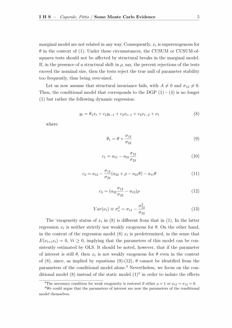
I H S – Caporale, Pittis / Some Monte Carlo Evidence 5
marginal model are not related in any way. Consequently, xt is superexogenous for
θ in the context of (1). Under these circumstances, the CUSUM or CUSUM-of-
squares tests should not be affected by structural breaks in the marginal model.
If, in the presence of a structural shift in ρ, say, the percent rejections of the tests
exceed the nominal size, then the tests reject the true null of parameter stability
too frequently, thus being over-sized.
Let us now assume that structural invariance fails, with A 6= 0 and σ12 6= 0.
Then, the conditional model that corresponds to the DGP (1) - (4) is no longer
(1) but rather the following dynamic regression:
yt = θ1xt + c1yt−1 + c2xt−1 + c3xt−2 + νt (8)
where
θ1 = θ +σ12
σ22
(9)
c1 = a11 − a21σ12
σ22
(10)
c2 = a12 −σ12
σ22
(a22 + ρ− a21θ)− a11θ (11)
c3 = (a22σ12
σ22
− a12)ρ (12)
V ar(νt) ≡ σ2ν = σ11 −
σ212
σ22
(13)
The ‘exogeneity status of xt in (8) is different from that in (1). In the latter
regression xt is neither strictly nor weakly exogenous for θ. On the other hand,
in the context of the regression model (8) xt is predetermined, in the sense that
E(νt+ixt) = 0, ∀i ≥ 0, implying that the parameters of this model can be con-
sistently estimated by OLS. It should be noted, however, that if the parameter
of interest is still θ, then xt is not weakly exogenous for θ even in the context
of (8), since, as implied by equations (9)-(12), θ cannot be identified from the
parameters of the conditional model alone.3 Nevertheless, we focus on the con-
ditional model (8) instead of the static model (1)4 in order to isolate the effects
3The necessary condition for weak exogeneity is restored if either ρ = 1 or a12 = σ12 = 0.4We could argue that the parameters of interest are now the parameters of the conditional
model themselves.

6 Caporale, Pittis / Some Monte Carlo Evidence – I H S
of structural change in the parameters of the marginal model on the properties
of the CUSUM test applied to the conditional model, when structural invariance
fails. The reason is that the dynamic model, as opposed to the static (1), is not
contaminated by other types of misspecification arising, say, from non-orthogonal
regressors and serially correlated errors.
The marginal model for xt can be written as:
xt = λ1xt−1 + λ2xt−2 + λ3yt−1 + e2t (14)
where
λ1 = ρ− a21θ + a22 (15)
λ2 = −a22ρ (16)
λ3 = a21 (17)
Assume now that the parameter ρ undergoes structural change as a result
of a change in the persistence of the regressor. The parameters of the marginal
model λ1 and λ2 will also change according to equations (9) and (10) respectively.
Furthermore, the parameters of the conditional model c2 and c3 will be affected
according to (11) and (12) respectively. In other words, the conditional model is
not structurally invariant with respect to these specific changes in the parameters
of the marginal model. Similarly, if the parameter of the marginal model λ3 = a21
changes (with all the other parameters in the DGP constant), this will induce
a change in the parameters of the conditional model c1 and c2. Moreover, if
the variance σ22 of the marginal model changes, then all the parameters of the
conditional model, including the variance of the conditional model σ2ν , will also
change according to (9)- (13). This means that, if a researcher applies the CUSUM
or CUSUM-of-squares test to the correct model (8), then he should expect a
rejection of the null hypothesis of parameter stability if one of the parameters
of the marginal process has shifted. In such a case, if the percent rejections of
the CUSUM or CUSUM-of-squares tests exceed their nominal sizes, this evidence
should be interpreted not as an indication that the tests are over-sized, but rather
in terms of their power, since the null hypothesis is obviously false.
Cointegration case: ρ = 1.
If ρ = 1 the DGP (1)-(4) becomes the triangular cointegration system anal-
ysed by Phillips and his co-authors in a series of papers (see, for example, Phillips

I H S – Caporale, Pittis / Some Monte Carlo Evidence 7
1988, Phillips and Hansen 1990). In this context, the effects of a non-exogenous
regressor are different from those in the stationary case. Applying OLS to (1)
yields superconsistent estimates of θ, regardless of the values of A and σ12. This
means that the OLS residuals u1t are consistent estimates of the regression er-
ror u1t. Nevertheless, ‘second-order’ asymptotic bias effects are present in the
asymptotic distribution of the OLS estimator. To be more precise, let us define
the long-run covariance matrix Ω and the one-sided covariance matrix ∆ given
by
Ω = (I − A)−1Σ(I − A>)−1 (18)
∆ = G(I − A>)−1 (19)
where Σ denotes the innovations covariance matrix of the VAR, and G is the
unconditional covariance matrix of ut given by
vecG = (I − A⊗ A)−1vecΣ (20)
One can now distinguish two nuisance parameters in the asymptotic distribution
of the OLS estimator. The first is the parameter, ω12/ω22, that describes the
”long-run correlation” effect, due to the non-diagonality of the long-run covariance
matrix Ω = [ωij] , i, j = 1, 2. The second is the parameter δ21 =∑∞
k=0 E(u20u1k),

8 Caporale, Pittis / Some Monte Carlo Evidence – I H S
that corresponds to the ”endogeneity” effect.5 The presence of these second-order
effects requires a modification of the standard CUSUM and CUSUM-of-squares
tests in order to correct for endogeneity and serial correlation, along the lines
suggested by Xiao and Phillips (2002). Nevertheless, it is easy to show that, if
a12 = a21 = σ12 = 0, the asymptotic nuisance parameters are zero and standard
OLS is optimal. In other words, the presence of a serially correlated error, that is
a11 6= 0, has no effects asymptotically on OLS, as shown by Kramer (1986) and
Park and Phillips (1988). Unlike in the stationary case, under the assumption that
the regressor is strictly exogenous, serial correlation has no asymptotic effects on
the null distributions of the CUSUM and CUSUM-of-squares test statistics.
As for structural invariance, similar considerations to those for the stationary
5Using some tedious algebra, it can be shown that ω12/ω22 and δ21 are related to theparameters of the VAR as follows:
ω12 = k21 σ12[(1− a11)(1− a22) + a12a21] + a12σ22(1− a11) + a21σ11(1− a22) (21)
ω22 = k21
a2
21σ11 + 2a21(1− a11)σ12 + (1− a11)2σ22
(22)
and
δ21 = k2[σ11a21ζ1 + σ12ζ2 + σ22a12ζ3] (23)
where
ζ1 = −a11 − a12a21a22 + a11a222 + a11a22 + a12a21a
222 − a11a
322 − a12a21 + (24)
+a212a
221 − a11a21a22a12
ζ2 = a212a
221 − 1 + a2
11 + a222 − a2
11a222 − a2
12a221a22 + a22 − a2
11a22 − a322 + (25)
a211a
322 − 2a11a
221a
212 − 2a21a22a12 + 2a2
11a21a22a12
ζ3 = −a11a21a12 − a22 + a211a22 + a11a21a22a12 + a2
22 − a211a
222 − 1 + a2
11 + (26)
a21a12 + a211a21a12 + a11a22 − a3
11a22
and
k1 = [det(I −A)]−1 (27)
k2 = [(−1 + detA)(det(I −A))2(1 + trA+ detA)]−1 (28)

I H S – Caporale, Pittis / Some Monte Carlo Evidence 9
case apply. The only difference is that structural change in the marginal process
cannot arise from a change in ρ, since now this parameter is fixed to unity. Of
course, one can consider a change in the parameter λ2 = −a22 affecting c2 and
c3, or in λ3 = a21 affecting c1 and c2, or in σ22 affecting all the parameters of the
conditional model.
3 Monte Carlo Results
This section reports on Monte Carlo simulations aimed at investigating the is-
sues discussed above and their implications for the size properties of the CUSUM
and CUSUM-of-squares tests. The only parameter kept fixed in all the experi-
ments that follow is θ = 1. We generate 2000 series of length 150, starting with
u10 = u20 = 0, and then discard the initial 50 observations, thus obtaining a
sample size of 100. We consider four different cases, and for each of them report
the percent rejections produced by the CUSUM and CUSUM-of-squares tests
for the hypothesis of parameter stability in the context of both the static (and
often heavily misspecified in a number of ways) regression (1) and the dynamic
regression (8).
Case I: Benchmark Case
Here we assume that A = 0, and σ12 = 0. We also set σ11 = σ22 = 1. This is a
case where the conditional expectation is equal to θxt. This means that the static
regression (1) is the correct model, whereas the dynamic (8) is over-specified. No
serial correlation or endogeneity effects are present. We set ρ = 0.5 (the stationary
case) and ρ = 1 (the cointegration case). The results are reported in Table 1. It
can be seen that the empirical sizes of both tests are close to their nominal 5%
value in both the stationary and the cointegration case. This is hardly surprising,
since, even with ρ = 1, the OLS estimator in the case of the correct model (1)
is the optimal estimator, and the modifications in the spirit of Xiao and Phillips
(2002) are redundant.
Case II: Non-exogenous Regressor
In this case, it is still assumed that A = 0, but σ12 now differs from zero.
This means that, in the context of the static regression (1), the regressor xt is
not predetermined, even though the error u1t is serially uncorrelated. On the
other hand, it is predetermined (and weakly exogenous for the parameters of
the conditional model, though not for θ) in the context of the ADL model (8),
and the regression error νt is, of course, serially uncorrelated. Nevertheless the

10 Caporale, Pittis / Some Monte Carlo Evidence – I H S
ADL model (8) is still over-specified, since the correct conditional expectation is
given by yt = θ1xt + c2x, where c2 = σ12
σ22ρ . In order to examine the effects of
different ”degrees” of endogeneity on the size properties of the tests under study,
we consider the following values of σ12 : σ12 = 0.3, 0.5, 0.7, 0.9. The results are
reported in Table 2, again for ρ = 0.5 and ρ = 1. They can be summarised as
follows:
1) The CUSUM-of-squares test is robust to the presence of σ12 6= 0 for both
ρ = 0.5 (the stationary case) and ρ = 1 (the cointegration case), since, although
applied to the misspecified equation (1), it does not exhibit size distortions. It
appears, therefore, that this source of misspecification does not affect the test in
either a stationary or a cointegrating environment.
2) A different picture emerges for the CUSUM test. Here there are important
differences between the two cases of a stationary or a cointegrating static regres-
sion. In the stationary case the size of the test applied to (1) remains close to the
nominal one for all values of σ12. If, however, ρ = 1, then the test is over-sized,
with the size distortion proportional to the endogeneity effect as measured by
σ12. For example, for σ12 = 0.7 the nominal size is 28.27 and 4.90 percent for
ρ = 1 and ρ = 0.5 respectively.
3) Nevertheless, the CUSUM test performs satisfactorily, even if ρ = 1, when
the test is applied to the dynamic model (8). The explanation is that this model,
unlike the static model (1), deals with the second-order endogeneity effects arising
from σ12 6= 0 in a parametric way, and hence they are not present in the residuals.
We also find that the non-parametric corrections for the CUSUM test, suggested
by Xiao and Phillips (2002), reduce the size distortions to a satisfactory level
(these results, not reported, are available on request).6 The implication is that,
when testing the stability of a cointegration model by means of the CUSUM test,
it is preferable to use the dynamic model (8) instead of the static model (1), unless
one is willing to undertake the additional computational burden entailed by the
Xiao and Phillips (2002) procedure. This is because the OLS-based CUSUM test
misinterprets the second-order effects as parameter instability, thus leading to
erroneous rejections of the null.
4) Finally, rather surprisingly, there appears to be no evidence that the CUSUM-
of-squares test is affected by second-order effects when applied to (1) for ρ = 1 -
a finding for which there is no obvious explanation.
Case III: Serially Correlated Regression Error
In this case it is again assumed that xt is predetermined in the context
6Note that these modifications work well even if the choice of the bandwidth parameter,needed to implement them, is not optimal.

I H S – Caporale, Pittis / Some Monte Carlo Evidence 11
of the static regression (1), which implies that a12 = σ12 = 0. We also set
a21 = 0. For this parameter settings, the conditional expectation is equal to
θxt + c1yt−1 + c2xt−1, where c1 = a11 and c2 = −a11θ. Of course, in the context of
the conditional model, xt is weakly exogenous for θ, and the regression error νt is
serially uncorrelated.7 In order to examine the effects of different degrees of serial
correlation on the size properties of the tests we consider the following values of
a11 : a11 = 0.3, 0.5, 0.7, 0.9. The results are reported in Table 3, again for ρ = 0.5
and ρ = 1. The main findings are the following:
1) In the stationary case ρ = 0.5, the effects of serial correlation on the size
(especially in the case of the CUSUM test) are significant. As the degree of serial
correlation increases, so does the size in the context of the static regression (1),
reaching the value of 86.77 and 68.37 percent for the CUSUM and CUSUM-of-
squares tests respectively. The implication is that, when testing for parameter
stability in the context of a regression model with a serially correlated error, the
researcher will erroneously infer that the model parameters are unstable.
2) In the cointegration case ρ = 1, a similar picture emerges. Both tests are
considerably over-sized, although slightly less so than in the stationary case.8
This is a rather surprising result in view of the fact that the effects of a serially
correlated error on the estimation of a cointegration parameter are asymptotically
negligible if the regressor is strictly exogenous (as in the present case - see Kramer
1986, Park and Phillips 1988). It should be noted that the Xiao and Phillips (2002)
modifications do not improve substantially the size behaviour of the tests (these
results are not reported, for reasons of space, but are available on request). For
example, for a11 = 0.7 the size of the OLS-based CUSUM test is 50.20 percent,
whereas the size of the ADL-based is 44.67 percent. This is hardly surprising,
since in this case a12 = σ12 = a21 = 0, and therefore both the nuisance parameters
ω12/ω22 and δ21 are already equal to zero, implying that there is no possible gain
from using the modifications.
3) In the context of the dynamic model (8) both tests (particularly the
CUSUM-of-squares) perform well in both environments, i.e. for ρ = 0.5 and
ρ = 1. Again, if one utilises the correct regression model, their performance is
satisfactory.
Case IV: (Lack of) Structural Invariance
The final set of experiments focuses on the role of structural invariance. One
would expect that, if this property holds, i.e. if changes in the parameters of
7Note that since a21 = 0, xt is also strongly exogenous for θ.8In the interpretation of Xiao and Phillips (2002), they reject too frequently the null hy-
pothesis of cointegration.

12 Caporale, Pittis / Some Monte Carlo Evidence – I H S
the marginal model do not cause corresponding changes in the parameters of
the conditional model, the percent rejections of the null hypothesis of parameter
constancy (of the conditional model) should not be higher than the nominal ones
for either the CUSUM or the CUSUM-of-squares tests. We consider the following
cases:
(a) Structural Invariance: A = 0, σ12 = 0. For this parameter setting the static
model (1) is the conditional model, whose parameters are θ and σ11. The marginal
model is xt = ρxt−1 + u2t, with parameters ρ and σ22. In this case structural
invariance holds. We introduce a shift in the parameter ρ of the marginal model,
which is set equal to 0.3 in the first half of the sample, and to 0.7 in the second
half. This shift in ρ does not affect the conditional parameters θ and σ11, and
hence should not affect the size properties of the tests under study. The results are
reported in Table 4A. It can be seen that both tests, whether they are applied
to the correct static (1) model or to the over-specified dynamic one (8), have
empirical sizes close to the corresponding nominal ones, confirming our prior that
the size properties should be robust to changes in the marginal parameters in the
presence of structural invariance.
We also adopt the following experimental design: we keep ρ constant for the
whole sample, and change the other parameter of the marginal model, i.e. σ22.
This allows us to examine the effects of a structural change in the marginal
model in both a stationary and a cointegrating framework (unlike in earlier cases
where ρ was allowed to change - then we could not analyse the latter case, since
cointegration requires ρ to be equal to one in the whole sample). Specifically, we
set σ22 = 1 in the first half of the sample, and σ22 = 2 in the second half. The
results are reported in Table 4B. The empirical sizes are close to the nominal
ones in both the stationary case ρ = 0.5 and the cointegration one ρ = 1, and for
both the static model (1) and the over-specified dynamic one (8). Again, despite a
change in the marginal process, structural invariance ensures that the tests retain
good size properties. Note that in the cases under study xt is superexogenous for
θ.
We also examine the robustness of the CUSUM and CUSUM-of-squares tests
to a very large shift in σ22 = 1, i.e. from 1 in the first half to 10 in the second half
of the sample. The results, reported in Table 4C, show that even such a sizeable
change in the parameters of the marginal model does not affect the properties of
the tests in the presence of structural invariance.
Further, we analyse the general case of structural invariance with A 6= 0
and σ12 6= 0, the parameter settings being such that the conditional model is
not affected by the shift in the underlying DGP parameters, whilst the marginal

I H S – Caporale, Pittis / Some Monte Carlo Evidence 13
model is. Specifically, consider the following parameter settings for the first half
of the sample: a11 = 0.4, a12 = 0.7, a22 = 0, a21 = 0.2, σ12 = 0.7, σ11 = σ22 = 1,
ρ = 0.5. Then the parameters of the marginal model will be equal to λ1 = 0.36,
λ2 = 0, λ3 = 0.2, σ22 = 1, whilst those of the conditional model will be equal to
θ1 = 1.4, c1 = 0.26, c2 = 0.168, c3 = −0.35 = σ2ν = 0.51. Assume that there is a
shift in the middle of the sample in the following parameters: a11 = 0.61, a12 =
0.98, a22 = 0.4, a21 = 0.5, σ12 = 1.4, σ11 = 1.49, σ22 = 2, ρ = 0.5. This will result
in λ1 = 0.55, λ2 = −0.2, λ3 = 0.5, σ22 = 2. As one can see, the parameters of the
marginal model have changed, whereas those of the conditional model have not -
in other words, structural invariance holds.
We have also investigated the effects of the same parameter shifts when ρ = 1
instead of ρ = 0.5, the values taken in the first subsample by the parameters of the
conditional model now being θ1 = 1.4, c1 = 0.26, c2 = −0.182, c3 = −0.70 = σ2ν =
0.51, and by those of the marginal model λ1 = 0.86, λ2 = 0.0, λ3 = 0.2, σ22 = 1.
The shifts do not affect the conditional model parameters, but the marginal ones
change to λ1 = 1.05, λ2 = −0.4, λ3 = 0.5, σ22 = 2 in the second subsample. The
results for both the stationary and the cointegration case are presented in Table
4D. It appears that structural invariance holds again, as the percent rejections
for both tests in the context of the correctly specified dynamic model (8) are
always close to the nominal ones. Let us analyse the consequences of using the
misspecified static model (1). It is apparent that its parameters, σ2u and θ, change
as a result of the shift. This is clearly the case for the former, as suggested by
equations (5)-(7). As for the latter, although the shift does not affect it directly,
it does affect the limiting parameter to which the OLS estimator applied to (1)
converges. This point can be illustrated by noting that, if one applies OLS to
(1), then this estimator, say θLS, will converge in probability to θ + θ, where θ
denotes the asymptotic bias due to the presence of a non-predetermined regressor.
It is easy to show that θ is a function of the parameters of the DGP changing
between regimes. Therefore, although θ itself does not change, θLS does as a result
of the shift in the DGP parameters, and so do the residuals on which the tests
are based. The static regression (1) is also misspecified in other ways. First, the
regression error u1t is serially correlated in both subsamples, with different degrees
of autocorrelation. For instance, the first and second autoregressive coefficients,
(a11 +a22) and (a11a22−a21a12) respectively, are equal to 0.4 and -0.14 in the first
half of the sample, and to 1.01 and -0.146 in the second. Second, the regressor xt
is not predetermined in either case (a12, σ12 6= 0 in both subsamples). Therefore,
one would expect both the CUSUM and CUSUM-of-squares tests to reject the
null when carried out in the context of the static regression (1). However, it

14 Caporale, Pittis / Some Monte Carlo Evidence – I H S
cannot be established whether such rejections are due to parameter instability
(the correct reason for rejecting), or to other types of misspecification (the wrong
reason). Indeed, the evidence presented in Table 4D confirms our conjecture that
the tests will reject the null hypothesis quite often, especially if ρ = 1. This is
in sharp contrast to their behaviour when applied to the correctly specified and
structurally invariant ADL model (8).
To summarise, these tests appear to reject the null when it is false (in the
case of the static model), and not to reject it when it is true (in the case of the
dynamic model). As already mentioned, the rejections in the former case might
reflect several types of misspecification, such as serial correlation (primarily) or
endogeneity, as well as parameter instability. We have reported earlier that au-
tocorrelated errors mainly affect the empirical size of both tests, whereas the
strongest effects of endogeneity occur in the case of the CUSUM test when coin-
tegration holds. These findings might be interpreted as an indication that the
tests under examination tend not to reject the null of parameter stability unless
some other form of misspecification is also present. Consequently, although it is
a desirable property that they should reject in the context of the static model
(which is indeed characterised by parameter instability), they are not informa-
tive about the specific reason behind such rejections, which could be one of many
forms of misspecification. Similarly, it is desirable that they should not reject
when applied to a correctly specified structurally invariant model (i.e. the ADL),
since the null in this case is true. But the question remains whether such be-
haviour is a consequence of a general tendency not to reject in the presence of
any type of misspecification (which might not be linked at all to parameter varia-
tion). To address these issues, we investigate next the performance of these tests
when the dynamic ADL model is not structurally invariant and the only source
of misspecification is instability in the parameters of the conditional model.
b) No Structural Invariance. Consider the following parameter settings for the
first half of the sample: a11 = 0.7, a12 = 0.7, a22 = 0, a21 = 0.3, σ12 = 0.7, σ11 =
σ22 = 1, ρ = 0.5. The corresponding conditional model parameters are equal to
θ1 = 1.4, c1 = 0.49, c2 = 0.007, c3 = −0.35, σ2ν = 0.51. Assume a permanent shift
in the middle of the sample in the following DGP parameters: a11 = 0.9, a12 =
0.0, a22 = 0.0, a21 = 0.7, σ12 = 0.0, σ11 = 4, σ22 = 2, ρ = 0.5. As a result, the
conditional model parameters will become equal to: θ1 = 0.7, c1 = 0.90, c2 =
-0.63, c3 = 0.00, σ2ν = 4, i.e. structural invariance does not hold. Consequently,
the CUSUM and CUSUM-of-squares tests should reject the null hypothesis of
parameter stability if applied to the dynamic regression (8). To put it differently,
the desirable behaviour of these tests in this particular case is that they should

I H S – Caporale, Pittis / Some Monte Carlo Evidence 15
”reject” as often as possible - and the percent rejections of the null should be
interpreted in terms of ”power” instead of size”. Note, once again, that here the
only form of misspecification is parameter instability: the ADL model does not
have either a serially correlated error or a non-predetermined regressor.
Similar considerations apply when the tests are applied to the static model (1).
This model is misspecified in several ways other than parameter instability: serial
correlation of the error ut (in both subsamples) and endogeneity of the regressor
(in the first subsample) are both present. Therefore, rejections of the null do not
lend themselves to a unique interpretation. The results for both the stationary
and the cointegration case are shown in Table 4E, and can be summarised as
follows:
(i) The CUSUM test lacks any power to detect the break that has occured in
the parameters of the correct (ADL) conditional model, this being true in both
the stationary and the cointegration case. In fact, its ”power” appears to be more
or less equal to its nominal size. On the contrary, the CUSUM-of-squares test
is extremely powerful and rejects the false null in 100% of the cases, whether a
stationary or a cointegration environment is considered. This is not a surprising
finding, given the very large step change in the variance of the regression error σ2v,
from 0.5 in the first to 4 in the second subsample. These results are in agreement
with those of Ploberger and Kramer (1990) and Hansen (1991), who argue that
neither test has asymptotic power to detect shifts in the slope parameters. Specif-
ically, the CUSUM test has local asymptotic power to detect shifts only in the
intercept, and the CUSUM-of-squares test only in the variance of the regression
error.
(ii) When the tests are applied to the misspecified static model (1), the
CUSUM test rejects more frequently (especially in the case of cointegration) than
it did in the context of the correctly specified ADL model. This can be seen as
further evidence that forms of misspecification other than parameter instability
cause the test to reject: here the null of parameter instability is correctly rejected,
but for the wrong reasons (serial correlation, endogeneity, etc.) The rejection fre-
quencies for the CUSUM-of-squares test are also high, but can more plausibly
be attributed to the correct reasons, as (a) it is the variance of u1t which has
changed, and therefore the test has a natural advantage over its CUSUM version
to reject for the right reasons, and (b) according to the results presented in Tables
2 and 3, it is less affected than the CUSUM test by misspecification in the form
of serial correlation or endogeneity.
Finally, we assume that the parameters of the DGP change in such a way as to
affect the slope parameters of the conditional model, but at the same time leave

16 Caporale, Pittis / Some Monte Carlo Evidence – I H S
the variance of the error σ2ν unaffected. The motivation is the following. In the
previous experiment, allowing σ2ν to change whilst keeping the intercept constant
meant that the CUSUM-of-squares test had an obvious advantage, as it is well
known that this test has more power to detect shifts in the former relative to
the CUSUM test, which performs better in detecting changes in the latter (see
Hansen, 1991). Therefore, a fairer comparison between the performance of the
two tests in the presence of a shift in the slope parameters of the conditional
model can be made by keeping the variance of the error constant. Specifically,
we assume that the parameters of the DGP in the first subsample are the same
as in the previous case, whilst in the second one they are set equal to: a11 = 0.9,
a12 = 0, a22 = 0, a21 = 0.7, σ12 = 1.732, σ11 = σ22 = 2. For the stationary case
ρ = 0.5. The parameters of the conditional model are equal to θ1 = 1.4, c1 =
0.49, c2 = 0.007, c3 = −0.35, σ2ν = 0.51 in the first subsample, and change to
θ1 = 1.566, c1 = 0.294, c2 = −0.638, c3 = 0, σ2ν = 0.51 in the second one. Similar
parameter shifts are introduced for the cointegration case ρ = 1. The results
are reported in Table 4F. It is apparent that the CUSUM-of-squares test has a
superior performance: it has satisfactory power to detect parameter instability
even when the conditional variance is kept constant. For instance, for ρ = 0.5,
and in the context of the correctly specified ADL model, the percent rejections
of the CUSUM and CUSUM-of-squares tests are 5.70 and 65.44 respectively. In
the cointegration case, with ρ = 1, the corresponding figures are 6.30 and 68.17.
Given the other types of robustness of the CUSUM-of-squares test already
documented, one can conclude that this test is more reliable to detect parameter
instability. It is important to note that its power to detect shifts in the slope
parameters of the ADL model (even when the conditional variance is constant)
increases further if the breaks occur later in the sample. For instance, if the shift
takes place after 75 (rather than 50, as previously) observations, its power is 94.56
and 94.98 percent in the stationary and cointegration case respectively. This is
in constrast to the findings of Kramer et al. (1988), who argued that ”power
decreases as the shift moves toward the end of the sample”. Instead, we find a
significantly lower power when the shift occurs after 25 observations (34.56 and
35.89 percent only in the two cases), i.e. as one moves towards the beginning of
the sample (the full set of results is not reported for reasons of space). Also note
that the power of this test is approximately equal to its nominal size regardless
of the point where the shift occurs.

I H S – Caporale, Pittis / Some Monte Carlo Evidence 17
4 Conclusions
This paper has investigated by means of Monte Carlo techniques the size proper-
ties of the CUSUM and CUSUM-of-squares tests (see Brown et al., 1975), which
are widely used in empirical applications because they are appropriate to test pa-
rameter instability against a variety of alternatives, but have been subjected to
various criticisms concerning their performance both in terms of size and power
(see, e.g., Kendall, 1975, Priestley, 1975, Kramer et al, 1988, Hansen, 1991). Our
findings, which have important implications for the applied researcher, suggest
the following.
The CUSUM-of-squares test is very robust to the presence of non-predetermined
(endogenous) regressors in both a stationary and a cointegration environment. In-
stead, the CUSUM test is robust only in the former case, whilst it is characterised
by large size distortions in the latter. These are proportional to the degree of cor-
relation between the regression error and the regressor. Further, serial correlation
has serious consequences in all cases, the CUSUM-of-squares test also being more
robust to the presence of weakly serially correlated errors.
The implication is that it is preferable to use these tests in the context of
a dynamic model of the ADL type, which is not affected by serial correlation
or non-predetermined regressors even if over-specified. In this case, the empiri-
cal sizes of both tests are close to the nominal ones, whether a stationary or a
cointegration environment is considered. This means that another advantage of
performing cointegration analysis using the ADL framework is the availability
of robust stability tests not requiring the modifications suggested by Xiao and
Phillips (2002). Although such tests are not directly interpretable as tests for
the null of cointegration, stability of the ADL parameter is a pre-requisite for
cointegration.
The two tests being considered are also robust to changes in the parameters
of the marginal process provided that structural invariance holds. In other words,
they do not misinterpret shifts in the marginal process as changes in the param-
eters of the conditional model, i.e. the frequency of a type-I error is not higher
than that implied by the nominal size. Structurally invariant parameters will be
obtained by employing the appropriate conditional model, i.e.the dynamic ADL
model, but not using a static model. For this reason, and also because such a
model is misspecified in ways that favour rejections, the percent rejections will
be higher.
When structural invariance fails, the CUSUM test is unable to detect parame-
ter instability even if this is substantial and present in both the slope parameters

18 Caporale, Pittis / Some Monte Carlo Evidence – I H S
and the variance of the regressor error. It tends to reject the null only if other
forms of misspecification are also present, and hence is more useful as a test for
serial correlation, say, than for parameter instability. Therefore, a rejection can
only be seen as a general indication of misspecification rather than a specific sign
of parameter variation. However, as is well known, this test does have power to
detect intercept shifts (see Hansen, 1991). By constrast, the CUSUM-of-squares
test is very powerful to detect changes in the conditional model parameters if the
variance of the regression error is included in the set of shifting parameters. Its
power is considerable even if this parameter is constant, especially towards the
end of the sample.
In brief, our findings imply that the CUSUM-of-squares test should always be
used in the context of a generalised dynamic ADL model, and never applied to a
static model. Its performance is satisfactory in both stationary and cointegration
environments. Importantly, it does not misinterpret shifts in the marginal process:
if it is carried out within a dynamic ADL model, rejections of the null are highly
likely to reflect actual parameter instability.
References
[1] Brown, R.L., Durbin, J. and J.M. Evans (1975), “Techniques for testing
the constancy of regression relationships over time,” Journal of the Royal
Statistical Society, Series B, 149-162.
[2] Engle, R.F., Hendry, D.F. and J.-F. Richard (1983), “Exogeneity,” Econo-
metrica, 51: 2, 277-304.
[3] Hansen , B.E. (1991) A Comparison of tests for parameter instability: An
examination of asymptotic local power, University of Rochester, working
paper.
[4] Hansen, B.E. (1992), “Tests for parameter instability in regressions with I(1)
processes,” Journal of Business & Economic Statistics, 10: 3, 321-335.
[5] Hansen, B. E. (2000), “Testing for structural change in conditional models,”
Journal of Econometrics, 97, 93-115.
[6] King, M.L. (1980), “Robust tests for spherical symmetry and their applica-
tion to least squares regression,” Annals of Statistics, 8, 1265-1271.
[7] King, M.L. (1985), “A point optimal test for autoregressive disturbances,”
Journal of Econometrics, 27, 21-37.

I H S – Caporale, Pittis / Some Monte Carlo Evidence 19
[8] King, M.L. (1988), “Towards a theory of point optimal testing,” Econometric
Reviews, 6, 169-218.
[9] King, M.L. and G.H. Hillier (1985), “Locally best invariant tests of the er-
ror covariance matrix of the linear regression model,” Journal of the Royal
Statistical Society, B 47, 98-102.
[10] Kramer, W. (1986), “Least-squares regression when the independent variable
follows an ARIMA process,” Journal of the American Statistical Association,
81, 150-154.
[11] Kramer, W., Ploberger, W., and R. Alt (1988), “Testing for structural change
in dynamic models,” Econometrica, 56, 1355-1369.
[12] LaMotte, L.R. and A. McWhorter (1978), “An exact test for the presence of
random walk coefficients ina linear regression model,” Journal of the Amer-
ican Statistical Association, 73, 816-820.
[13] Leybourne, S.J. and B.P.M. McCabe (1989), “On the distribution of some
test statistics for coefficient constancy,” Biometrika, 76, 169-177.
[14] Moryson, M. (1998), Testing for Random Walk Coefficients in Regression
and State Space Models, Physica-Verlag, Berlin.
[15] Nyblom, J. (1989), “Testing the constancy of parameters over time,” Journal
of the American Statistical Association, 84, 223-230.
[16] Nyblom, J. and T. Makelainen (1983), “Comparison of tests for the pres-
ence of random walk coefficients in a simple linear model,” Journal of the
American Statistical Association, 78, 856-864.
[17] Park, J.Y. and P.C.B. Phillips (1988), “Statistical inference in regressions
with integrated processes,” Econometric Theory, 4, 468-497.
[18] Phillips, P.C.B. (1988), “Reflections on Econometric Methodology,” Eco-
nomic Record, 64, 334-359.
[19] Phillips, P.C.B. and B.E. Hansen (1990), ”Statistical inference in instrumen-
tal regressions with I(1) processes,” Review of Economic Studies, 57, 99-125.
[20] Ploberger, W. and W. Kramer (1990), “The local power of the CUSUM and
CUSUM of squares tests,” Econometric Theory, 6, 335-347.
[21] Ploberger, W. and W. Kramer (1992), “The CUSUM test with OLS residu-
als,” Econometrica, 60, 271-285.

20 Caporale, Pittis / Some Monte Carlo Evidence – I H S
[22] Priestley, M.B. (1975), discussion of Brown, R.L., Durbin, J. and J.M. Evans
(1975), “Techniques for testing the constancy of regression relationships over
time,” Journal of the Royal Statistical Society, Series B, 166-168.
[23] Quandt, R.E. (1975), discussion of Brown, R.L., Durbin, J. and J.M. Evans
(1975), “Techniques for testing the constancy of regression relationships over
time,” Journal of the Royal Statistical Society, Series B, 183-184.
[24] Smith, A.F.M. (1975), discussion of Brown, R.L., Durbin, J. and J.M. Evans
(1975), “Techniques for testing the constancy of regression relationships over
time,” Journal of the Royal Statistical Society, Series B, 175-177.
[25] Xiao, Z. and P.C.B. Phillips (2002), “A CUSUM Test for Cointegration Us-
ing Regression Residuals,” No 1329, Cowles Foundation Discussion Papers,
Cowles Foundation, Yale University.

I H S – Caporale, Pittis / Some Monte Carlo Evidence 21
TABLE 1 Benchmark Case, A=0, Σ=Ι.
Percent Rejections of the Null Hypothesis of Parameter Stability
CUSUM CUSUM-SQ ρ=0.5
OLS 4.20 5.43 ADL 4.37 5.83
ρ=1 OLS 3.77 5.43 ADL 4.50 5.83
TABLE 2 Endogeneity: A=0, σ12≠0
Percent Rejections of the Null Hypothesis of Parameter Stability CUSUM CUSUM-SQ ρ=0.5, σ12=0.3
OLS 4.03 5.43 ADL 4.07 5.77
ρ=1, σ12=0.3 OLS 8.17 4.77 ADL 5.63 5.87
ρ=0.5, σ12=0.5 OLS 4.63 5.67 ADL 4.20 5.90
ρ=1, σ12=0.5 OLS 15.00 5.63 ADL 4.97 5.50
ρ=0.5, σ12=0.7 OLS 4.90 5.87 ADL 4.73 6.17
ρ=1, σ12=0.7 OLS 28.27 5.13 ADL 4.70 5.50
ρ=0.5, σ12=0.9 OLS 7.40 5.70 ADL 4.20 5.50
ρ=1, σ12=0.9 OLS 46.53 5.50 ADL 4.57 5.27

22 Caporale, Pittis / Some Monte Carlo Evidence – I H S
TABLE 3 Serial Correlation: a11≠0
Percent Rejections of the Null Hypothesis of Parameter Stability CUSUM CUSUM-SQ ρ=0.5, a11=0.3
OLS 16.40 8.67 ADL 5.07 5.90
ρ=1, a11=0.3 OLS 14.07 9.03 ADL 5.07 6.33
ρ=0.5, a11=0.5 OLS 31.73 15.80 ADL 5.53 6.17
ρ=1, a11=0.5 OLS 27.97 16.50 ADL 6.13 6.37
ρ=0.5, a11=0.7 OLS 56.11 33.83 ADL 6.80 6.30
ρ=1, a11=0.7 OLS 50.20 34.20 ADL 8.00 6.37
ρ=0.5, a11=0.9 OLS 86.77 68.37 ADL 10.10 6.40
ρ=1, a11=0.9 OLS 79.43 68.93 ADL 11.73 6.57

I H S – Caporale, Pittis / Some Monte Carlo Evidence 23
TABLE 4
Structural Breaks Percent Rejections of the Null Hypothesis of Parameter Stability
A. Structural Invariance Holds, Α=0 σ12=0
ρ: 0.3 →0.7 at 50th observation
CUSUM CUSUM-SQ OLS 3.80 5.37 ADL 4.93 6.00
B. Structural Invariance Holds, Α=0 σ12=0 σ22: 1 →2 at 50th observation
CUSUM CUSUM-SQ ρ=0.5
OLS 4.20 5.43 ADL 4.37 5.83
ρ=1 OLS 3.77 5.40 ADL 4.50 5.86
C. Structural Invariance Holds, Α=0 σ12=0 σ22: 1 →10 at 50th observation
Cusum Cusum-SQ ρ=0.5
OLS 5.10 5.99 ADL 5.65 6.24
ρ=1 OLS 4.87 5.87 ADL 5.76 6.87

24 Caporale, Pittis / Some Monte Carlo Evidence – I H S
D. Structural Invariance Holds, A≠0, σ12≠0
a11: 0.4 →0.61 σ11: 1 .0→1.49 a12: 0.7 →0.98 σ12: 0.7 →1.40 a21: 0.2 →0.50 σ22: 1.0 →2.00 a22: 0.0 →0.40
ALL at 50th observation
CUSUM CUSUM-SQ ρ=0.5
OLS 55.41 41.34 ADL 5.80 5.86
ρ=1 OLS 81.20 94.39 ADL 5.15 5.02
E. Structural Invariance Fails
a11: 0.7 →0.90 σ11: 1.0 →4.00 a12: 0.7 →0.00 σ12: 0.7 →0.00 a21: 0.3 →0.70 σ22: 1.0 →2.00 a22: 0.0 →0.00
ALL at 50th observation Cusum Cusum-SQ ρ=0.5
OLS 59.86 100 ADL 5.80 100
ρ=1 OLS 90.11 95.30 ADL 7.03 100

I H S – Caporale, Pittis / Some Monte Carlo Evidence 25
F. Structural Invariance Fails
(Conditional variance remains constant)
a11: 0.7 →0.90 σ11: 1.0 →2.00 a12: 0.7 →0.00 σ12: 0.7 →1.732 a21: 0.3 →0.70 σ22: 1.0 →2.00 a22: 0.0 →0.00
ALL at 50th observation CUSUM CUSUM-SQ ρ=0.5
OLS 79.66 69.39 ADL 5.70 65.44
ρ=1 OLS 93.33 78.55 ADL 6.30 68.17
G. Structural Invariance Fails (Conditional variance remains constant)
a11: 0.7 →0.90 σ11: 1.0 →2.00 a12: 0.7 →0.00 σ12: 0.7 →1.732 a21: 0.3 →0.70 σ22: 1.0 →2.00 a22: 0.0 →0.00
ALL at 75th observation CUSUM CUSUM-SQ ρ=0.5
OLS 70.19 81.89 ADL 5.40 94.56
ρ=1 OLS 93.82 78.95 ADL 6.50 94.98

Authors: Guglielmo Maria Caporale, Nikitas Pittis Title: Robustness of the CUSUM and CUSUM-of-Squares Tests to Serial Correlation, Endogeneity
and Lack of Structural Invariance: Some Monte Carlo Evidence Reihe Ökonomie / Economics Series 157 Editor: Robert M. Kunst (Econometrics) Associate Editors: Walter Fisher (Macroeconomics), Klaus Ritzberger (Microeconomics) ISSN: 1605-7996 © 2004 by the Department of Economics and Finance, Institute for Advanced Studies (IHS), Stumpergasse 56, A-1060 Vienna • +43 1 59991-0 • Fax +43 1 59991-555 • http://www.ihs.ac.at

ISSN: 1605-7996