rock, rattle and slide - politecnico di...
TRANSCRIPT

Rock, Rattle and Slidebifurcation theory for piecewise-smooth systems
Alan Champneys
Department of Engineering Mathematics, University of Bristol
Mario di Bernardo, Chris Budd, Piotr Kowalczyk
Arne Nordmark Harry Dankowicz, Gabor Licsko, Csaba Bazso . . .
Milan 4/6/09 – p. 1

Contents
1: Nonsmoothness and discontinuity-inducedbifurcation
Milan 4/6/09 – p. 2

Contents
1: Nonsmoothness and discontinuity-inducedbifurcation
2: grazing bifurcation in impacting systemsEx. i. a rattling heating valve
Milan 4/6/09 – p. 2

Contents
1: Nonsmoothness and discontinuity-inducedbifurcation
2: grazing bifurcation in impacting systemsEx. i. a rattling heating valve
3: grazing & corner bifurcation in PWS systemsEx. ii. extended model for stick-slip
Milan 4/6/09 – p. 2
Contents
1: Nonsmoothness and discontinuity-inducedbifurcation
2: grazing bifurcation in impacting systemsEx. i. a rattling heating valve
3: grazing & corner bifurcation in PWS systemsEx. ii. extended model for stick-slip
4: sliding bifurcation in Filippov systemsEx. iii. relay controller
5: nonsmooth impact laws with frictionEx. iv. Painlevé paradox of falling rod
6: Conclusion
Milan 4/6/09 – p. 2
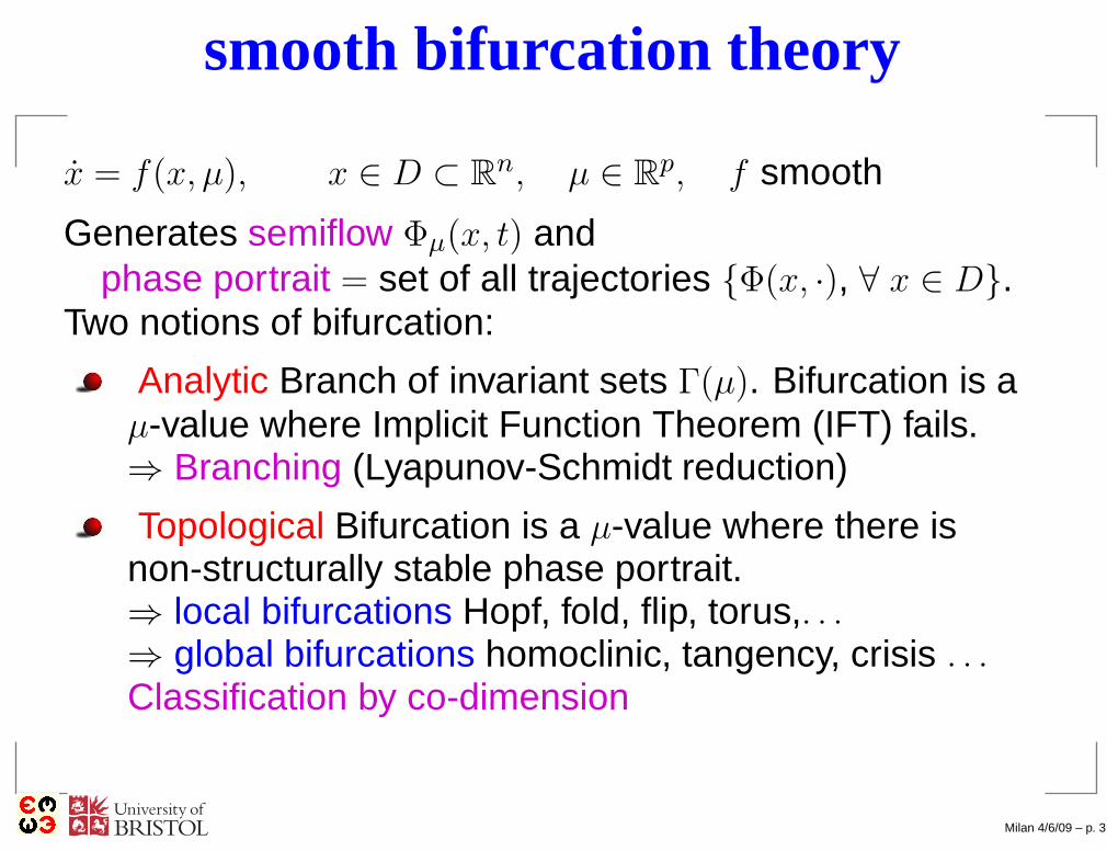
smooth bifurcation theory
x = f(x, µ), x ∈ D ⊂ Rn, µ ∈ R
p, f smooth
Generates semiflow Φµ(x, t) andphase portrait = set of all trajectories {Φ(x, ·), ∀ x ∈ D}.
Milan 4/6/09 – p. 3

smooth bifurcation theory
x = f(x, µ), x ∈ D ⊂ Rn, µ ∈ R
p, f smooth
Generates semiflow Φµ(x, t) andphase portrait = set of all trajectories {Φ(x, ·), ∀ x ∈ D}.
Two notions of bifurcation:
Milan 4/6/09 – p. 3

smooth bifurcation theory
x = f(x, µ), x ∈ D ⊂ Rn, µ ∈ R
p, f smooth
Generates semiflow Φµ(x, t) andphase portrait = set of all trajectories {Φ(x, ·), ∀ x ∈ D}.
Two notions of bifurcation:
Analytic Branch of invariant sets Γ(µ). Bifurcation is aµ-value where Implicit Function Theorem (IFT) fails.⇒ Branching (Lyapunov-Schmidt reduction)
Milan 4/6/09 – p. 3
smooth bifurcation theory
x = f(x, µ), x ∈ D ⊂ Rn, µ ∈ R
p, f smooth
Generates semiflow Φµ(x, t) andphase portrait = set of all trajectories {Φ(x, ·), ∀ x ∈ D}.
Two notions of bifurcation:
Analytic Branch of invariant sets Γ(µ). Bifurcation is aµ-value where Implicit Function Theorem (IFT) fails.⇒ Branching (Lyapunov-Schmidt reduction)
Topological Bifurcation is a µ-value where there isnon-structurally stable phase portrait.⇒ local bifurcations Hopf, fold, flip, torus,. . .⇒ global bifurcations homoclinic, tangency, crisis . . .Classification by co-dimension
Milan 4/6/09 – p. 3

smooth bifurcation theory
x = f(x, µ), x ∈ D ⊂ Rn, µ ∈ R
p, f smooth
Generates semiflow Φµ(x, t) andphase portrait = set of all trajectories {Φ(x, ·), ∀ x ∈ D}.
Two notions of bifurcation:
Analytic Branch of invariant sets Γ(µ). Bifurcation is aµ-value where Implicit Function Theorem (IFT) fails.⇒ Branching (Lyapunov-Schmidt reduction)
Topological Bifurcation is a µ-value where there isnon-structurally stable phase portrait.⇒ local bifurcations Hopf, fold, flip, torus,. . .⇒ global bifurcations homoclinic, tangency, crisis . . .Classification by co-dimension
IFT & struct. stabilty need continuity & smoothness . . .
Milan 4/6/09 – p. 3
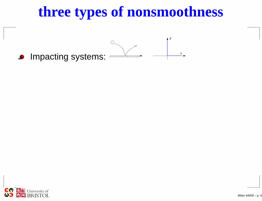
three types of nonsmoothness
Impacting systems:
F
x
Milan 4/6/09 – p. 4

three types of nonsmoothness
Impacting systems:
F
x
Milan 4/6/09 – p. 4
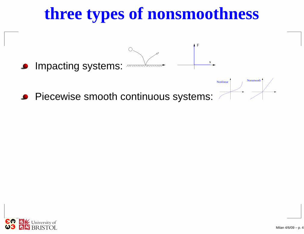
three types of nonsmoothness
Impacting systems:
F
x
Piecewise smooth continuous systems:
Nonlinear Nonsmooth
Milan 4/6/09 – p. 4

three types of nonsmoothness
Impacting systems:
F
x
Piecewise smooth continuous systems:
Nonlinear Nonsmooth
Y Y YX X X
T
PQ
a
ug
tlz
R
al
ug
b
T
tgz
P
Q
Milan 4/6/09 – p. 4

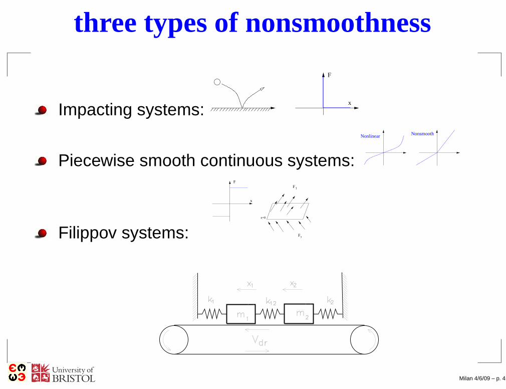
three types of nonsmoothness
Impacting systems:
F
x
Piecewise smooth continuous systems:
Nonlinear Nonsmooth
Filippov systems:
F
x
F1
F2
x=0
Milan 4/6/09 – p. 4
three types of nonsmoothness
Impacting systems:
F
x
Piecewise smooth continuous systems:
Nonlinear Nonsmooth
Filippov systems:
F
x
F1
F2
x=0
Milan 4/6/09 – p. 4
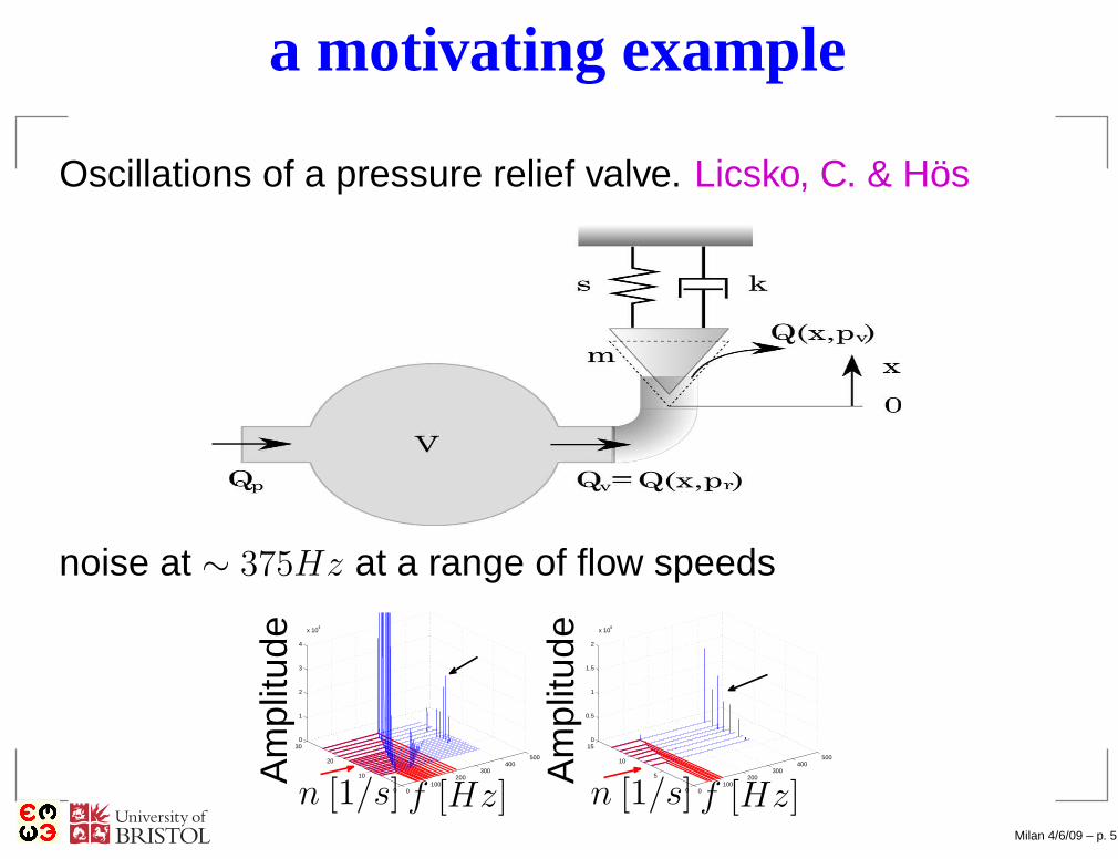
a motivating example
Oscillations of a pressure relief valve. Licsko, C. & Hös
noise at ∼ 375Hz at a range of flow speeds
0100
200300
400500
0
10
20
300
1
2
3
4
x 104
n [1/s] f [Hz]
Am
plitu
de
0100
200300
400500
0
5
10
150
0.5
1
1.5
2
x 106
n [1/s] f [Hz]
Am
plitu
de
Milan 4/6/09 – p. 5

a simple (dimensionless) model
y1 = y2
y2 = −κy2 − (y1 + δ) + y3
y3 = β (q −√y3y1)
y1 > 0 valve displacement; y2 valve velocity, y3 pressure
β valve spring stiffness; δ valve pre-stressq, flow rate; κ, fluid damping
at y1 = 0 apply a Newtonian restitution law:
y2(t+∗) = −ry2(t
−
∗)
Low κ ⇒ limit cycles between 2 Hopf bifs q = qmin, qmax.
Milan 4/6/09 – p. 6

brute force numerics
κ = 1.25, β = 20, δ = 10 (representative of experiment)
01
23
45
6 −10
−5
0
5
100
10
20
30
40
50
vel
disp
pres
−20
24
68
10 −10
0
10
20
0
10
20
30
40
50
60
70
80
vel
disp
pres
−20
24
68 −10
0
10
200
10
20
30
40
50
60
vel
disp
pres
−10
12
34
5 −10
−5
0
5
10
0
5
10
15
20
25
30
35
40
vel
disp
pres
−0.5
0
0.5
1 −4
−2
0
2
40
5
10
15
20
veldisp
pres
q
Chaotic rattling due to Grazing events at q ≈ 7.54, 5.95
Milan 4/6/09 – p. 7
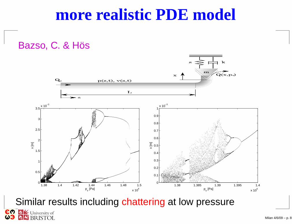
more realistic PDE model
Bazso, C. & Hös
1.38 1.4 1.42 1.44 1.46 1.48 1.5
x 106
0
0.5
1
1.5
2
2.5
3
3.5x 10
−3
pv [Pa]
x [m
]
1.38 1.385 1.39 1.395 1.4
x 106
0
0.1
0.2
0.3
0.4
0.5
0.6
0.7
0.8
0.9
1x 10
−3
pv [Pa]
x [m
]
Similar results including chattering at low pressureMilan 4/6/09 – p. 8

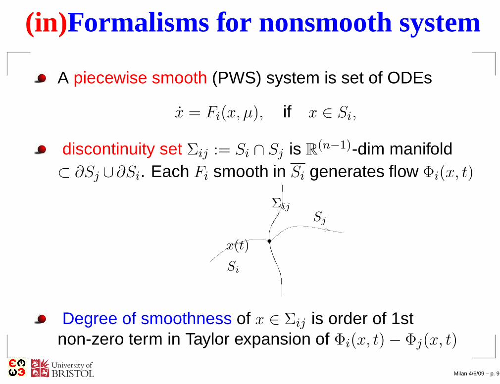
(in)Formalisms for nonsmooth system
A piecewise smooth (PWS) system is set of ODEs
x = Fi(x, µ), if x ∈ Si,
Milan 4/6/09 – p. 9

(in)Formalisms for nonsmooth system
A piecewise smooth (PWS) system is set of ODEs
x = Fi(x, µ), if x ∈ Si,
discontinuity set Σij := Si ∩ Sj is R(n−1)-dim manifold
⊂ ∂Sj ∪∂Si. Each Fi smooth in Si generates flow Φi(x, t)
x(t)
Si
Sj
Σij
Milan 4/6/09 – p. 9

(in)Formalisms for nonsmooth system
A piecewise smooth (PWS) system is set of ODEs
x = Fi(x, µ), if x ∈ Si,
discontinuity set Σij := Si ∩ Sj is R(n−1)-dim manifold
⊂ ∂Sj ∪∂Si. Each Fi smooth in Si generates flow Φi(x, t)
x(t)
Si
Sj
Σij
Degree of smoothness of x ∈ Σij is order of 1stnon-zero term in Taylor expansion of Φi(x, t) − Φj(x, t)
Milan 4/6/09 – p. 9
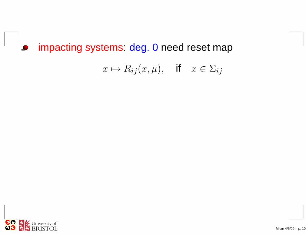
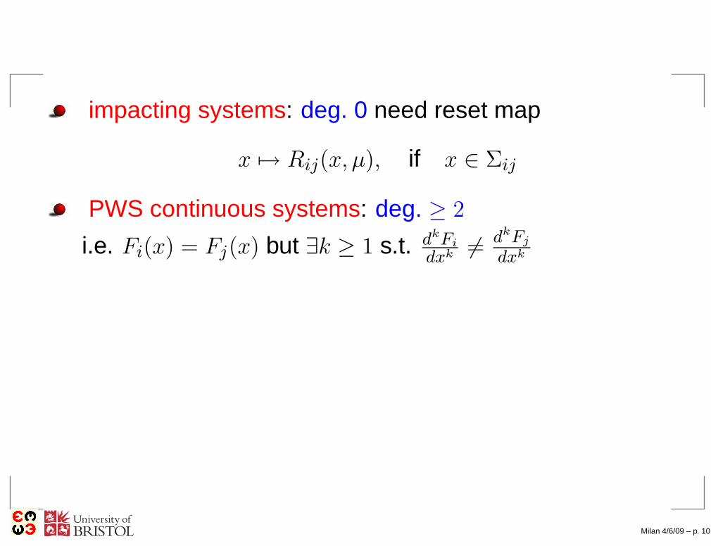
impacting systems: deg. 0 need reset map
x 7→ Rij(x, µ), if x ∈ Σij
Milan 4/6/09 – p. 10
impacting systems: deg. 0 need reset map
x 7→ Rij(x, µ), if x ∈ Σij
PWS continuous systems: deg. ≥ 2
i.e. Fi(x) = Fj(x) but ∃k ≥ 1 s.t. dkFi
dxk 6= dkFj
dxk
Milan 4/6/09 – p. 10
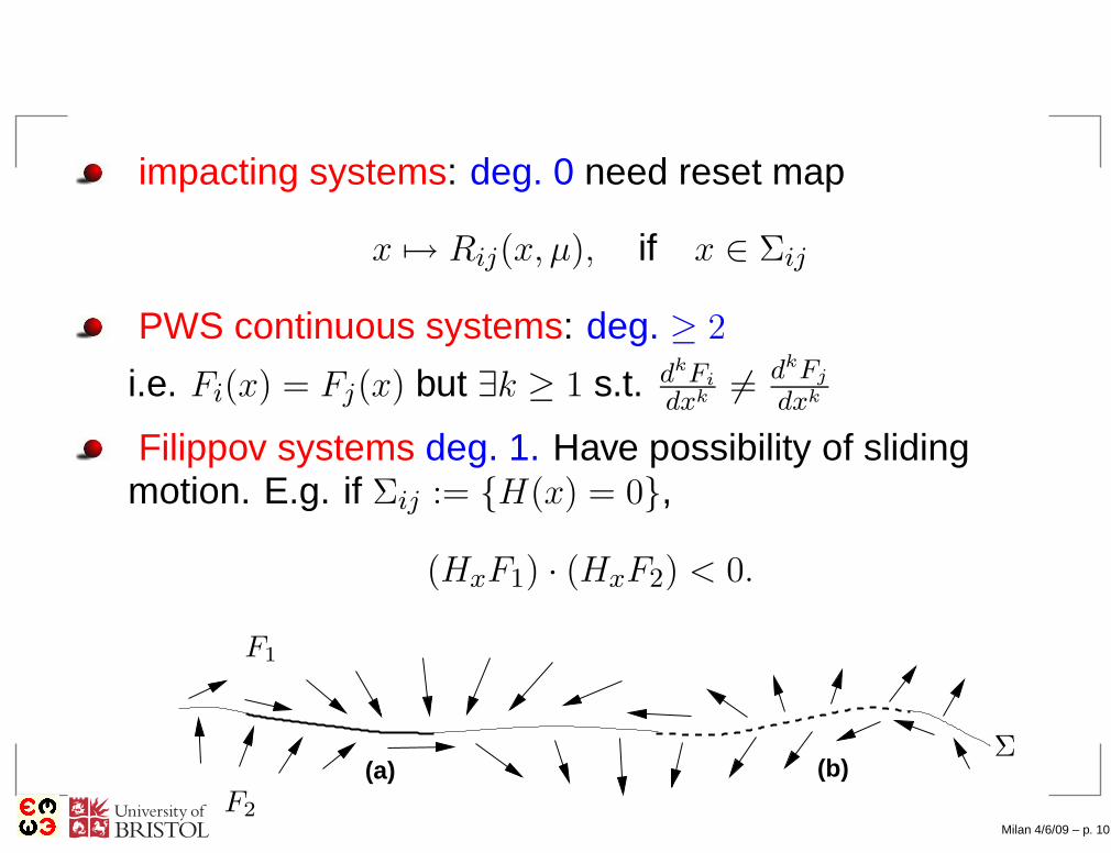
impacting systems: deg. 0 need reset map
x 7→ Rij(x, µ), if x ∈ Σij
PWS continuous systems: deg. ≥ 2
i.e. Fi(x) = Fj(x) but ∃k ≥ 1 s.t. dkFi
dxk 6= dkFj
dxk
Filippov systems deg. 1. Have possibility of slidingmotion. E.g. if Σij := {H(x) = 0},
(HxF1) · (HxF2) < 0.
(a) (b)
F1
F2
Σ
Milan 4/6/09 – p. 10
bifurcation
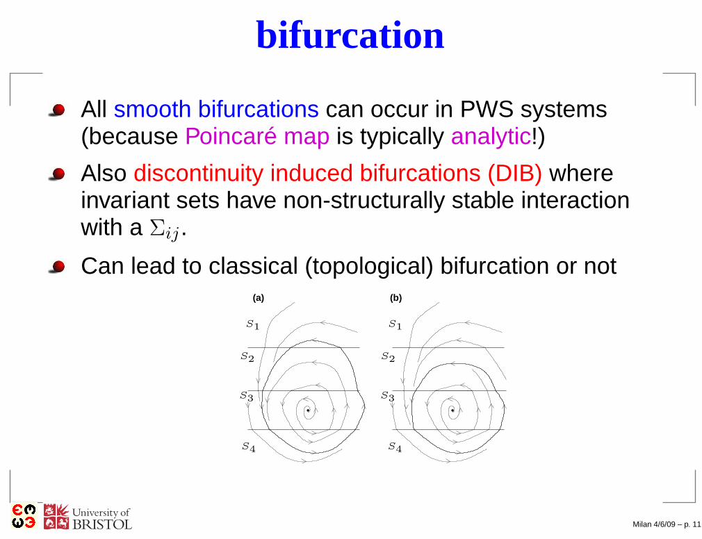
All smooth bifurcations can occur in PWS systems(because Poincaré map is typically analytic!)
Milan 4/6/09 – p. 11
bifurcation
All smooth bifurcations can occur in PWS systems(because Poincaré map is typically analytic!)
Also discontinuity induced bifurcations (DIB) whereinvariant sets have non-structurally stable interactionwith a Σij .
Milan 4/6/09 – p. 11
bifurcation
All smooth bifurcations can occur in PWS systems(because Poincaré map is typically analytic!)
Also discontinuity induced bifurcations (DIB) whereinvariant sets have non-structurally stable interactionwith a Σij .
Can lead to classical (topological) bifurcation or not(a) (b)
S1
S2
S3
S4
S1
S2
S3
S4
Milan 4/6/09 – p. 11

bifurcation
All smooth bifurcations can occur in PWS systems(because Poincaré map is typically analytic!)
Also discontinuity induced bifurcations (DIB) whereinvariant sets have non-structurally stable interactionwith a Σij .
Can lead to classical (topological) bifurcation or not(a) (b)
S1
S2
S3
S4
S1
S2
S3
S4
idea topological DIB ⇐ PW structural stabilityMilan 4/6/09 – p. 11

types of DIB
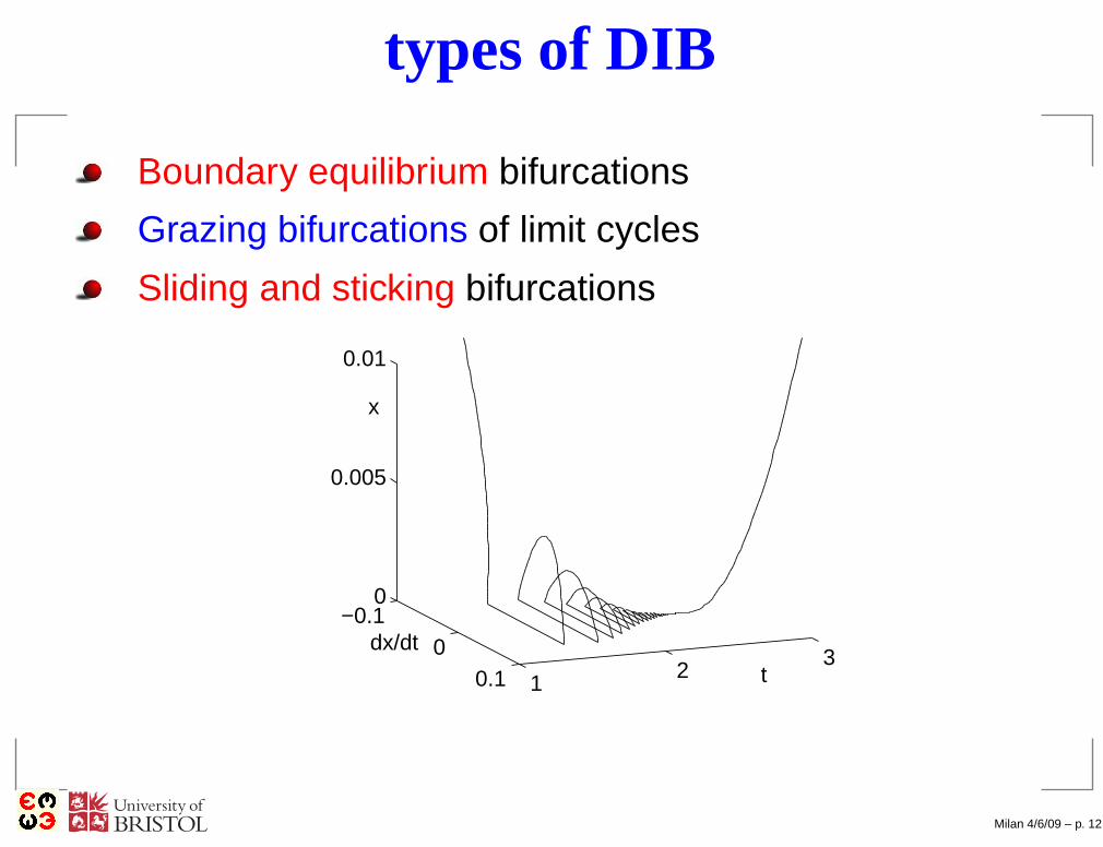
Boundary equilibrium bifurcations
mlz
b
mezmgz
Milan 4/6/09 – p. 12

types of DIB
Boundary equilibrium bifurcations
Grazing bifurcations of limit cyclesc
mezmlz
mgz
Milan 4/6/09 – p. 12

types of DIB
Boundary equilibrium bifurcations
Grazing bifurcations of limit cycles
Sliding and sticking bifurcations
Milan 4/6/09 – p. 12
types of DIB
Boundary equilibrium bifurcations
Grazing bifurcations of limit cycles
Sliding and sticking bifurcations
−0.10
0.1 12
3
0
0.005
0.01
t
dx/dt
x
Milan 4/6/09 – p. 12

types of DIB
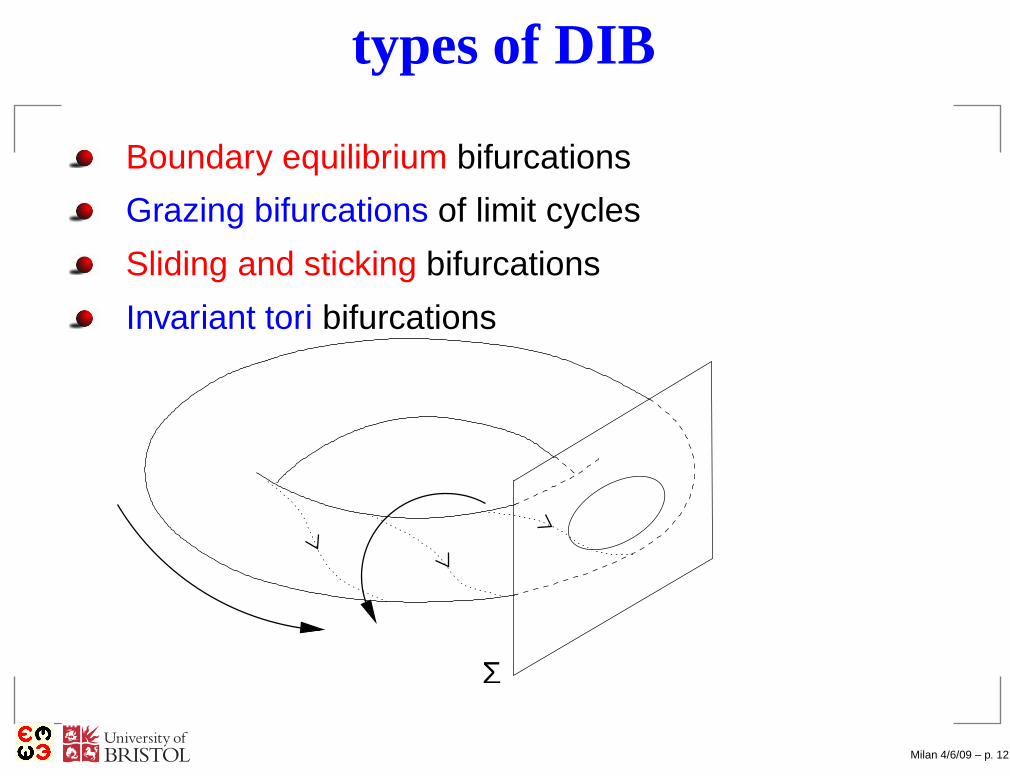
Boundary equilibrium bifurcations
Grazing bifurcations of limit cycles
Sliding and sticking bifurcations
Invariant tori bifurcations
Milan 4/6/09 – p. 12
types of DIB
Boundary equilibrium bifurcations
Grazing bifurcations of limit cycles
Sliding and sticking bifurcations
Invariant tori bifurcations
Σ
Milan 4/6/09 – p. 12
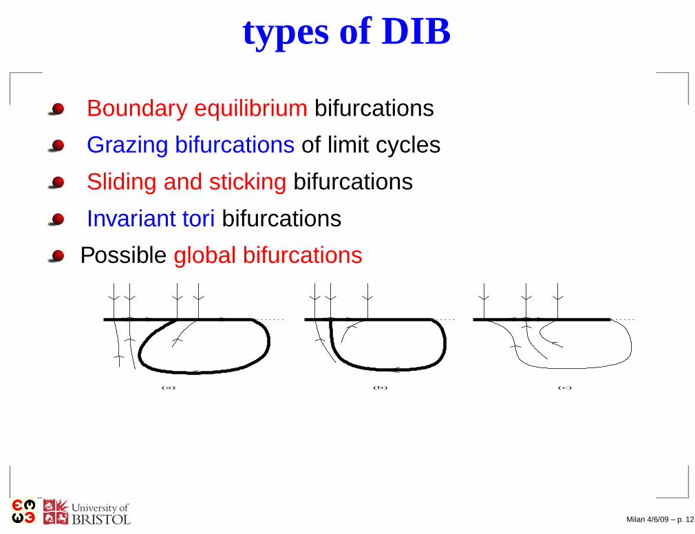
types of DIB
Boundary equilibrium bifurcations
Grazing bifurcations of limit cycles
Sliding and sticking bifurcations
Invariant tori bifurcations
Possible global bifurcations
Milan 4/6/09 – p. 12
types of DIB
Boundary equilibrium bifurcations
Grazing bifurcations of limit cycles
Sliding and sticking bifurcations
Invariant tori bifurcations
Possible global bifurcations
(c)(a) (b)
Milan 4/6/09 – p. 12
this talk: periodic orbit DIBs
Goal: Catalogue & unfold codim-1 possibilities.E.g. ‘grazing bifurcation’: [Nordmark]
Milan 4/6/09 – p. 13
this talk: periodic orbit DIBs
Goal: Catalogue & unfold codim-1 possibilities.E.g. ‘grazing bifurcation’: [Nordmark]
Derive map close to DIB as composition of smoothPoincaré map Pπ and discontinuity mapping PDM
Pπ
Πp(t)
Σ : {H(x) = 0}PDM
Milan 4/6/09 – p. 13
this talk: periodic orbit DIBs
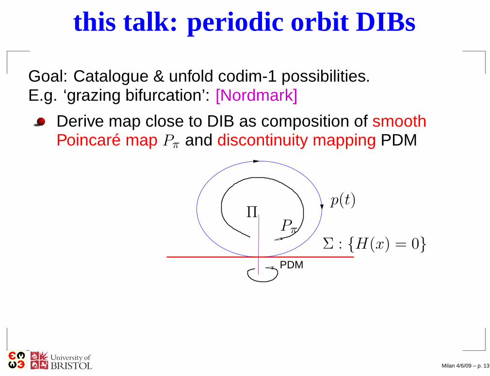
Goal: Catalogue & unfold codim-1 possibilities.E.g. ‘grazing bifurcation’: [Nordmark]
Derive map close to DIB as composition of smoothPoincaré map Pπ and discontinuity mapping PDM
Pπ
Πp(t)
Σ : {H(x) = 0}PDM
Use results on border collisions of maps to classifydynamics [Feigin] [Yorke, Banergee et al]
Milan 4/6/09 – p. 13

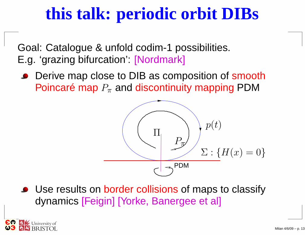
this talk: periodic orbit DIBs
Goal: Catalogue & unfold codim-1 possibilities.E.g. ‘grazing bifurcation’: [Nordmark]
Derive map close to DIB as composition of smoothPoincaré map Pπ and discontinuity mapping PDM
Pπ
Πp(t)
Σ : {H(x) = 0}PDM
Use results on border collisions of maps to classifydynamics [Feigin] [Yorke, Banergee et al]
Nb. piecewise linear (PWL) flow 6⇒ PWL mapMilan 4/6/09 – p. 13

2. Grazing bifurcation in impact systems
cf. Theory of impact oscillators: [Peterka] 1970s,[Thompson & Ghaffari], [Shaw & Holmes] 1980s,[Budd et al], [Nordmark] 1990s.
Consider single impact surface Σ := {H(x) = 0}with impact law:
x+ = R(x−) = x− + W (x−)HxF (x−)
W is smooth function and HxF (x−) is ‘velocity’. e.g.
W = −(1 + r)Hx ⇒ Newton’s ‘restitution law’
More complex impact laws are possible, e.g. impactwith friction (see later)
Milan 4/6/09 – p. 14
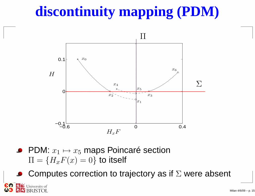
discontinuity mapping (PDM)
−0.6 0 0.4−0.1
0
0.1
HxF
H
x2 x3
x5
x1
x4
x0
x6
Σ
Π
PDM: x1 7→ x5 maps Poincaré sectionΠ = {HxF (x) = 0} to itself
Computes correction to trajectory as if Σ were absent
Milan 4/6/09 – p. 15

explicit form of PDM
cf. [Fredrickson & Nordmark]
x 7→{
x if H(x) ≥ 0
x + β(x, y)y if H(x) < 0
}
where β = −√
2a
(
W − (HxF )xW
aF
)
+ O(y2),
where y =√−H and
a(x) = d2H/dt2 = (HxF )xF = HxxFF + HxFxF
⇒ square root map
Milan 4/6/09 – p. 16

Proof is by Taylor expansion of flow in (x, y) and IFT
Milan 4/6/09 – p. 17
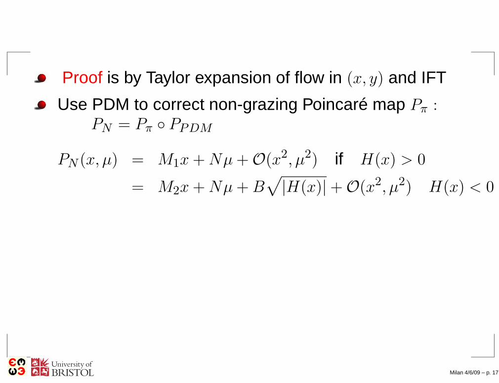
Proof is by Taylor expansion of flow in (x, y) and IFT
Use PDM to correct non-grazing Poincaré map Pπ :PN = Pπ ◦ PPDM
PN (x, µ) = M1x + Nµ + O(x2, µ2) if H(x) > 0
= M2x + Nµ + B√
|H(x)| + O(x2, µ2) H(x) < 0
Milan 4/6/09 – p. 17
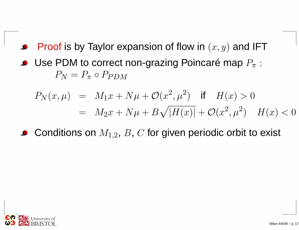
Proof is by Taylor expansion of flow in (x, y) and IFT
Use PDM to correct non-grazing Poincaré map Pπ :PN = Pπ ◦ PPDM
PN (x, µ) = M1x + Nµ + O(x2, µ2) if H(x) > 0
= M2x + Nµ + B√
|H(x)| + O(x2, µ2) H(x) < 0
Conditions on M1,2, B, C for given periodic orbit to exist
Milan 4/6/09 – p. 17
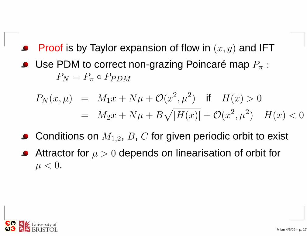
Proof is by Taylor expansion of flow in (x, y) and IFT
Use PDM to correct non-grazing Poincaré map Pπ :PN = Pπ ◦ PPDM
PN (x, µ) = M1x + Nµ + O(x2, µ2) if H(x) > 0
= M2x + Nµ + B√
|H(x)| + O(x2, µ2) H(x) < 0
Conditions on M1,2, B, C for given periodic orbit to exist
Attractor for µ > 0 depends on linearisation of orbit forµ < 0.
Simplest case:λ1 real leading eigenvalue of M1 . . ., then dynamics isdetermined by 1D map:
Milan 4/6/09 – p. 17

dynamics of 1D map
f(x) =√
µ − x + λ1µ x < µ, f(x) = λ1x x > µ,
1. 2/3 < |λ1| < 1: robust chaotic attractor size ∼ √µ.
2. If 1/4 < |λ1| < 2/3 alternating series of chaos andperiod-n orbits, n → ∞ as µ → 0.
3. 0 < |λ1| < 1/4: just period-adding cascade
Milan 4/6/09 – p. 18

return to Ex.i: valve rattle
Two grazing bifurcation events q = 7.54, q = 5.95
q = 5.95: λ1 < 0 ⇒ discontinuous jump in attractorq = 7.54: λ1 = 0.8537 ⇒ jump to chaos. Iterate map
7.4 7.45 7.5 7.55 7.6 7.65−0.1
−0.05
0
0.05
0.1
0.15
0.2
0.25
y[−
]
Milan 4/6/09 – p. 19

3. DIBs in PWS continuous systems
Simplest case: grazing bifurcationAnalyse using discontinuity mapping: PDM
��������
��������
��������
��������
��������
��������
��������
��������
��
����
��
δ∆
Σx x
fx
0xε
01tst 2t ft
S
S
ε
DiscontinuityMap
0
-
+
ΠΠ 1
2
Π
-
Milan 4/6/09 – p. 20
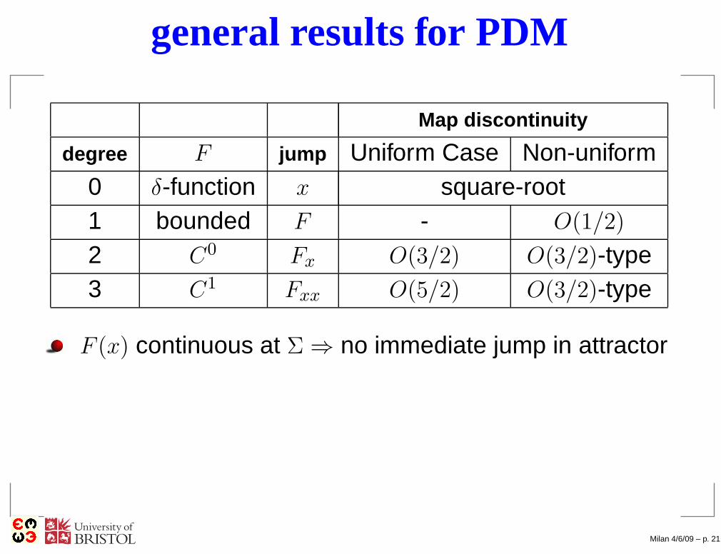
general results for PDM
Map discontinuity
degree F jump Uniform Case Non-uniform0 δ-function x square-root1 bounded F - O(1/2)
2 C0 Fx O(3/2) O(3/2)-type3 C1 Fxx O(5/2) O(3/2)-type
F (x) continuous at Σ ⇒ no immediate jump in attractor
Milan 4/6/09 – p. 21
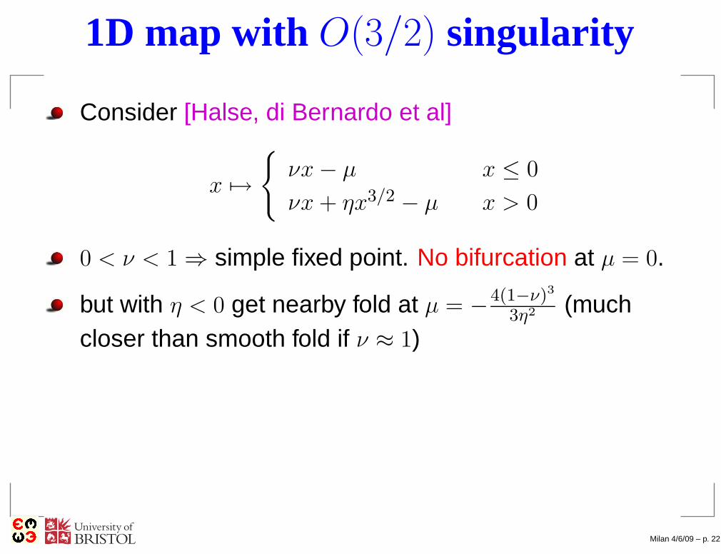
1D map with O(3/2) singularity
Consider [Halse, di Bernardo et al]
x 7→{
νx − µ x ≤ 0
νx + ηx3/2 − µ x > 0
0 < ν < 1 ⇒ simple fixed point. No bifurcation at µ = 0.
but with η < 0 get nearby fold at µ = −4(1−ν)3
3η2 (muchcloser than smooth fold if ν ≈ 1)
Milan 4/6/09 – p. 22
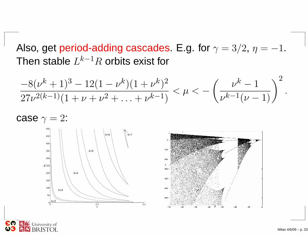
Also, get period-adding cascades. E.g. for γ = 3/2, η = −1.Then stable Lk−1R orbits exist for
−8(νk + 1)3 − 12(1 − νk)(1 + νk)2
27ν2(k−1)(1 + ν + ν2 + . . . + νk−1)< µ < −
(
νk − 1
νk−1(ν − 1)
)2
.
case γ = 2:
0 0.2 0.40
50
100
150
200
250
300
350
400
450
500
α
βµ
k=2
k=3
k=4
k=5
k=6 k=7
Milan 4/6/09 – p. 23
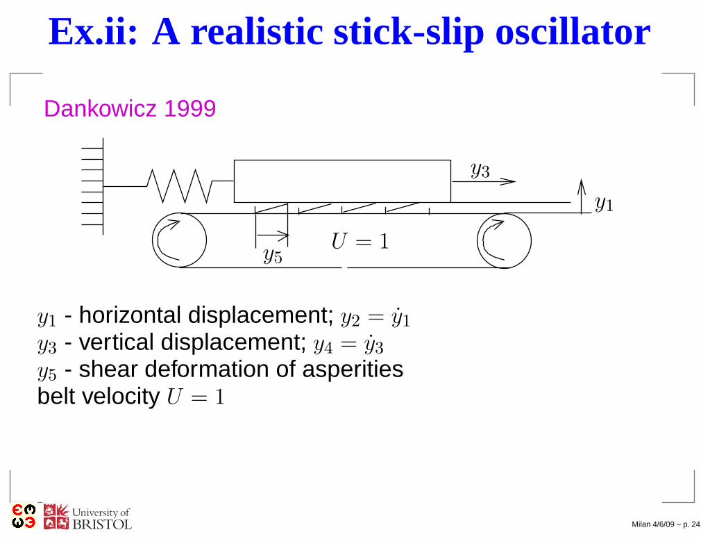
Ex.ii: A realistic stick-slip oscillator
Dankowicz 1999
U = 1
y1
y3
y5
y1 - horizontal displacement; y2 = y1
y3 - vertical displacement; y4 = y3
y5 - shear deformation of asperitiesbelt velocity U = 1
Milan 4/6/09 – p. 24

equations of motion
y1 = y2,
y2 = −1 +[
1 − γU |1 − y4|y2 + βU2(1 − y4)2√
K(y1)]
ey1−d,
y3 = y4,
y4 = −sy3 +
√gσ
Ue−d
[
µ(y5e−y1 − 1) + αU2S(y1, y4)
]
,
y5 =1
τ[(1 − y4) − |1 − y4|y5],
where K(y1) = 1 − y1−d∆ ,
S(y1, y4) = (1 − y4)|1 − y4|K(y1)e−y1 − 1 + d
∆ .
⇒ PWS continuous across discontinuity boundary y4 = 1.
Milan 4/6/09 – p. 25

grazing bifurcation analysis
Dankowicz & Nordmark 20003 successive zooms of bifurcation diagram:
Milan 4/6/09 – p. 26

grazing bifurcation analysis
Dankowicz & Nordmark 2000Simulation (left) and iteration of DM (right)
in local map co-ordinates ∼ y4 × 10−4
Milan 4/6/09 – p. 26

4. Sliding DIBs in Filippov systems
Kowalczyk, Nordmark, diBernardoFour possible DIB involving collision of limit cycle withsliding boundary ∂Σ−; see Mike Jeffrey’s talk
(a)
S
S
+
−
B AC
crossing sliding(b)
S+
C
B
A
grazing sliding
(c) S−
S+
A
C
B
switching sliding(d) C
S+
B
A
adding slidingMilan 4/6/09 – p. 27

Unfold with discontinuity mapping Di Bernardo, Kowalczyk,Nordmark
Bifurcation type DM leading-order term Map singularity
crossing sliding ε2 + O(ε3) 2grazing sliding ε + O(ε3/2) 1
switching sliding ε3 + O(ε4) 3adding sliding ε2 + O(ε5/2) 2
Maps are non-invertible on one side
Only grazing sliding ⇒ jump in attractor
Milan 4/6/09 – p. 28

Ex.iv: a relay control system
x = Ax − Bsgn(y), y = CT x,
A =
0
B
B
@
−a1 1 0
−a2 0 1
−a3 0 0
1
C
C
A
, B =
0
B
B
@
b1
b2
b3
1
C
C
A
, CT =
0
B
B
@
1
0
0
1
C
C
A
T
.
Complex dynamics:
−2
0
2
−4
0
4−0.1
0
0.1
x1
x2x3 z
z
z
0p1
m4
p2
m2
p4m0p1
b = (1,−2, 1)T , a31 = −5 a21 = −99.3, and(a) a11 = 1.206, 1.35, periodic; (b) nearby, chaotic
Milan 4/6/09 – p. 29
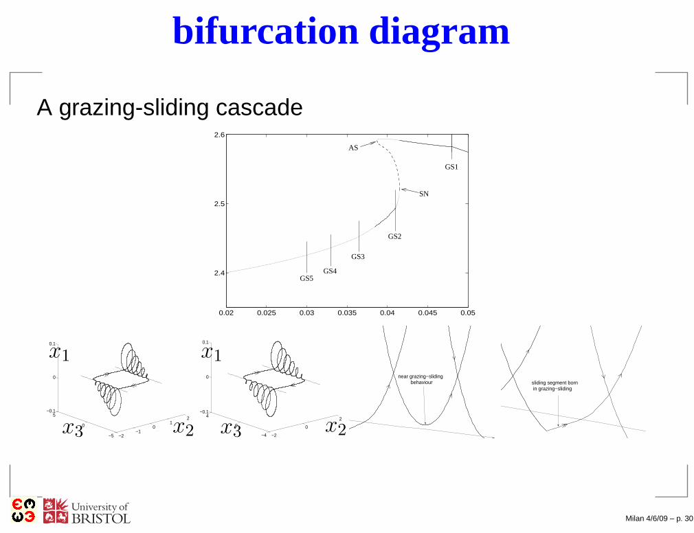
bifurcation diagram
A grazing-sliding cascade
0.02 0.025 0.03 0.035 0.04 0.045 0.05
2.4
2.5
2.6
SN
GS5GS4
GS3
GS2
GS1
AS
−2−1
01
2
−5
0
5−0.1
0
0.1
x2
x3
x1
x1
x2x3 −2
0
2
−4
0
4−0.1
0
0.1
x2
x3
x1
x1
x2x3
near grazing−sliding behaviour sliding segment born
in grazing−sliding
Milan 4/6/09 – p. 30

5. Impact with friction
Dankowicz Nordmark & C.
q ∈ Rn, with rigid contact in 2D + Coulomb friction
M (q, t) q = f(q, q, t) + λT cTu (q, t) + λNcT
v (q, t),
Scalar constraint y ≥ 0, y ∈ R normal distance;λN ≥ 0, λT ∈ R normal and tangential forces;
Coulomb friction, |λT | ≤ µλN , λT = −sign(u)µλN if u 6= 0
e.g. rod & table Painlevé 1905, Brogliato et al.
P1
P2
¸N
¸T
X
Y
Sx
Sy
Rµ
(x; y)
¹
u
¡¹
¡¸T =¸N
Milan 4/6/09 – p. 31
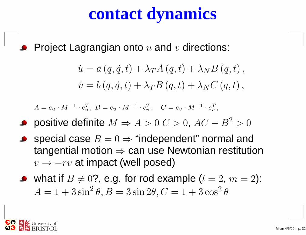
contact dynamics
Project Lagrangian onto u and v directions:
u = a (q, q, t) + λT A (q, t) + λNB (q, t) ,
v = b (q, q, t) + λT B (q, t) + λNC (q, t) ,
A = cu · M−1· cT
u , B = cu · M−1· cT
v , C = cv · M−1· cT
v ,
positive definite M ⇒ A > 0 C > 0, AC − B2 > 0
special case B = 0 ⇒ “independent” normal andtangential motion ⇒ can use Newtonian restitutionv → −rv at impact (well posed)
what if B 6= 0?, e.g. for rod example (l = 2, m = 2):A = 1 + 3 sin2 θ,B = 3 sin 2θ, C = 1 + 3 cos2 θ
Milan 4/6/09 – p. 32
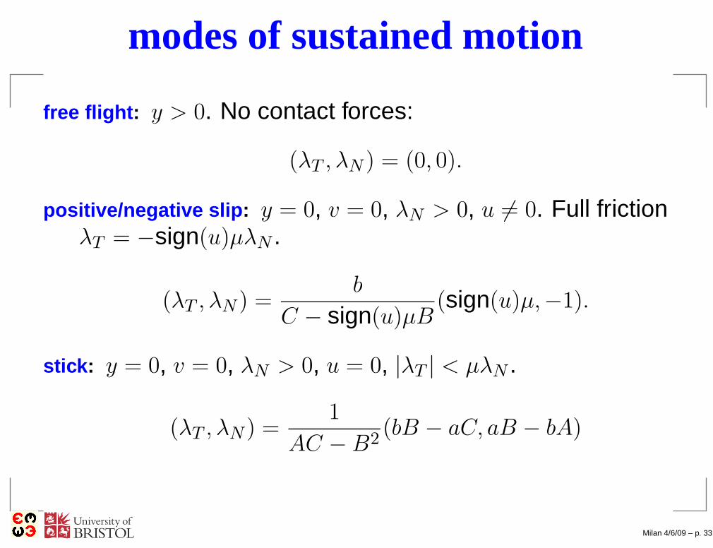
modes of sustained motion
free flight : y > 0. No contact forces:
(λT , λN ) = (0, 0).
positive/negative slip : y = 0, v = 0, λN > 0, u 6= 0. Full frictionλT = −sign(u)µλN .
(λT , λN ) =b
C − sign(u)µB(sign(u)µ,−1).
stick : y = 0, v = 0, λN > 0, u = 0, |λT | < µλN .
(λT , λN ) =1
AC − B2(bB − aC, aB − bA)
Milan 4/6/09 – p. 33
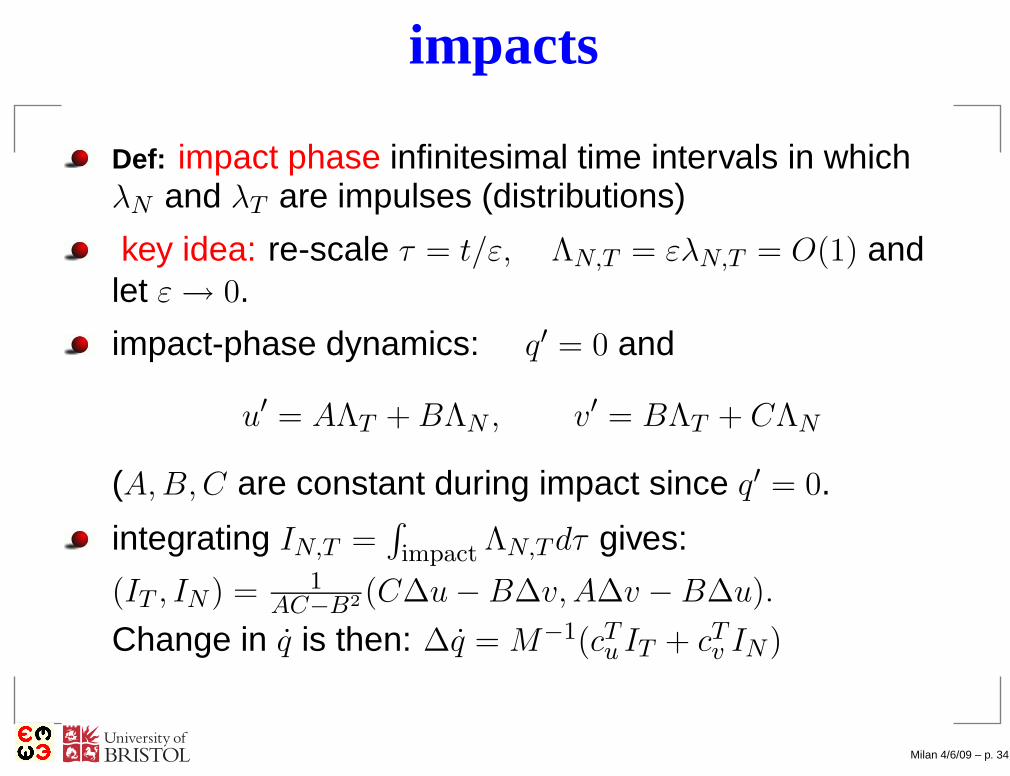
impacts
Def: impact phase infinitesimal time intervals in whichλN and λT are impulses (distributions)
key idea: re-scale τ = t/ε, ΛN,T = ελN,T = O(1) andlet ε → 0.
impact-phase dynamics: q′ = 0 and
u′ = AΛT + BΛN , v′ = BΛT + CΛN
(A,B,C are constant during impact since q′ = 0.
integrating IN,T =∫
impact ΛN,T dτ gives:
(IT , IN ) = 1AC−B2 (C∆u − B∆v,A∆v − B∆u).
Change in q is then: ∆q = M−1(cTu IT + cT
v IN )
Milan 4/6/09 – p. 34
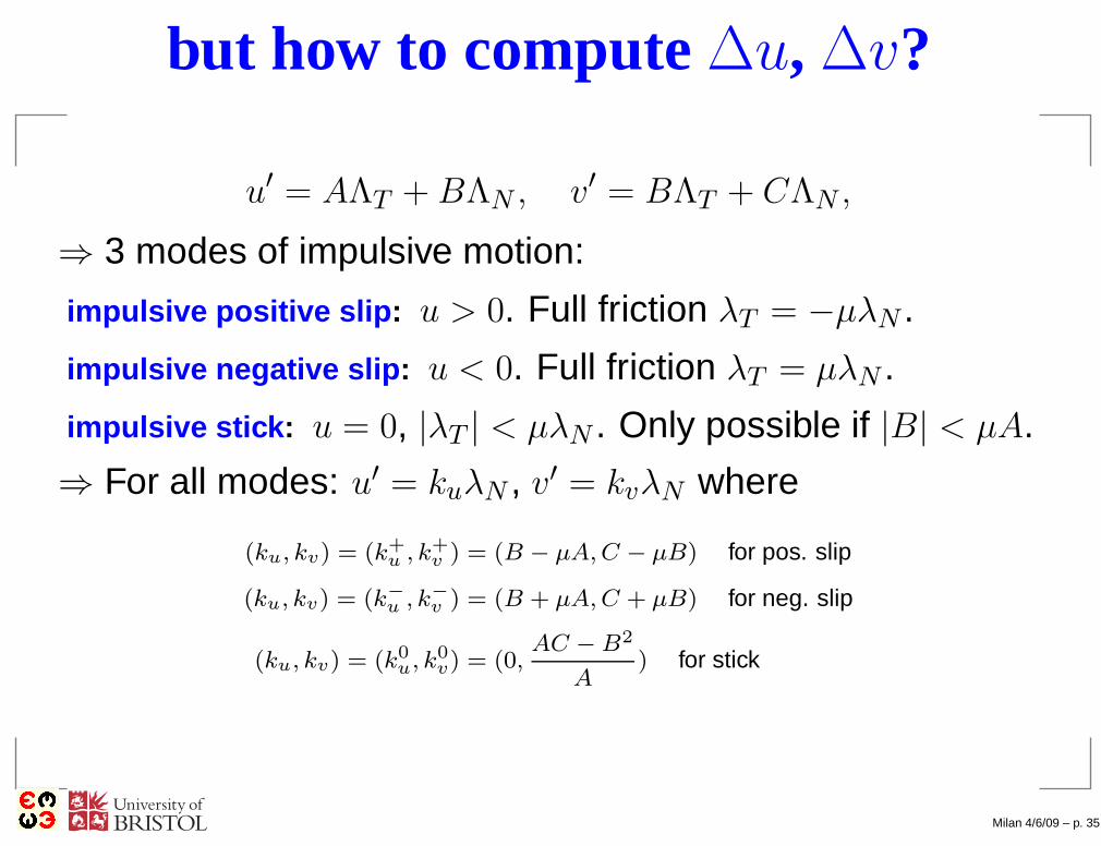
but how to compute∆u, ∆v?
u′ = AΛT + BΛN , v′ = BΛT + CΛN ,
⇒ 3 modes of impulsive motion:
impulsive positive slip : u > 0. Full friction λT = −µλN .
impulsive negative slip : u < 0. Full friction λT = µλN .
impulsive stick : u = 0, |λT | < µλN . Only possible if |B| < µA.
⇒ For all modes: u′ = kuλN , v′ = kvλN where
(ku, kv) = (k+u , k+
v ) = (B − µA, C − µB) for pos. slip
(ku, kv) = (k−
u , k−
v ) = (B + µA, C + µB) for neg. slip
(ku, kv) = (k0u, k0
v) = (0,AC − B2
A) for stick
Milan 4/6/09 – p. 35
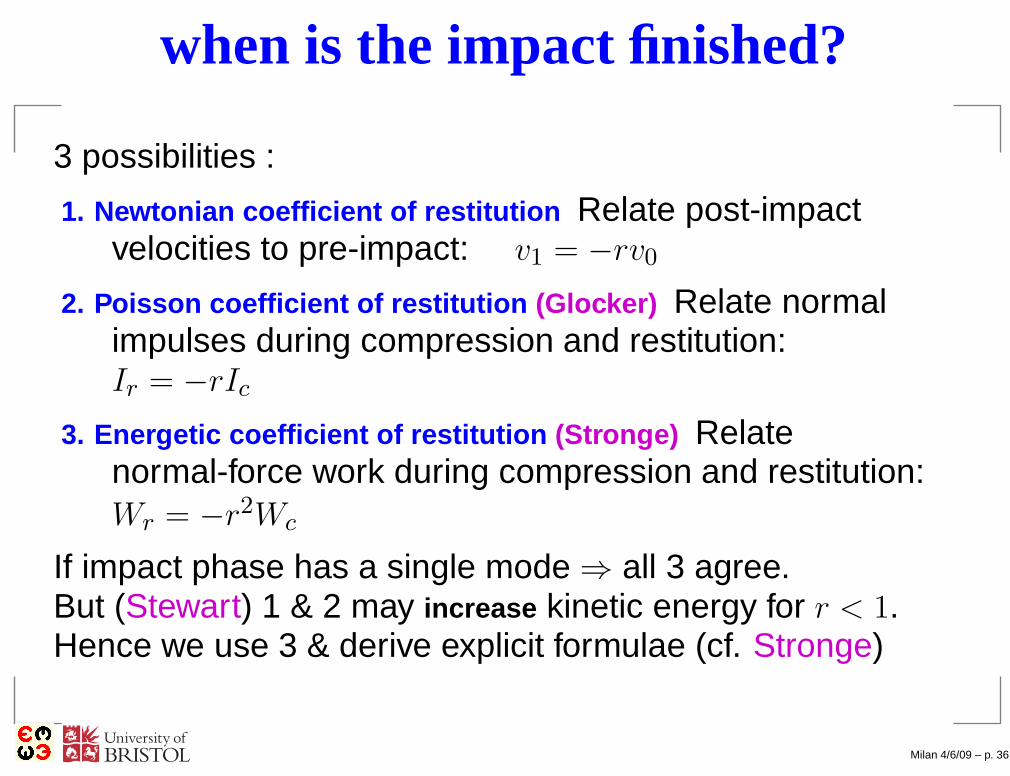
when is the impact finished?
3 possibilities :
1. Newtonian coefficient of restitution Relate post-impactvelocities to pre-impact: v1 = −rv0
2. Poisson coefficient of restitution (Glocker) Relate normalimpulses during compression and restitution:Ir = −rIc
3. Energetic coefficient of restitution (Stronge) Relatenormal-force work during compression and restitution:Wr = −r2Wc
If impact phase has a single mode ⇒ all 3 agree.But (Stewart) 1 & 2 may increase kinetic energy for r < 1.Hence we use 3 & derive explicit formulae (cf. Stronge)
Milan 4/6/09 – p. 36
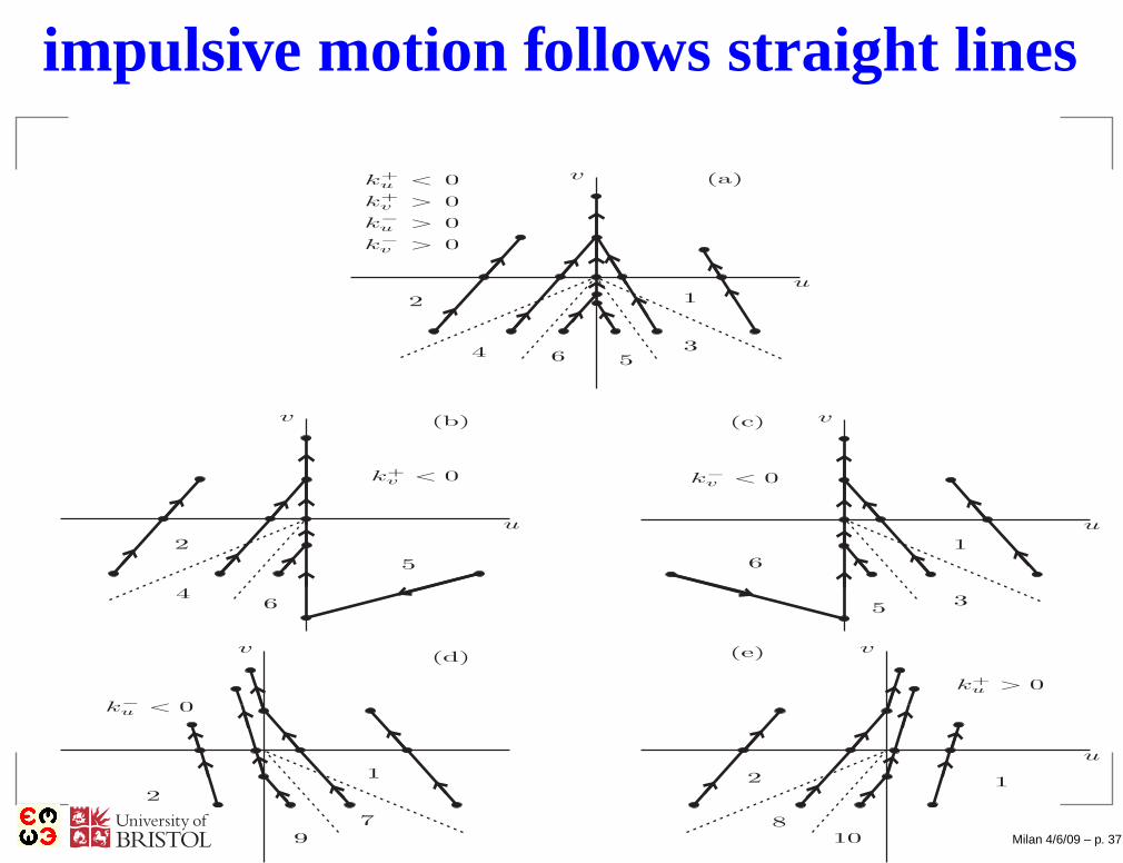
impulsive motion follows straight lines
u
v
12
810
k+u > 0
u
v
2
4
5
6
k+v < 0
1
2
79
k¡
u < 0
u
v
1
35
6
k¡
v < 0
u
v
12
3456
<
>
>
k+u
k+v
k¡
u
k¡
v >
0
0
0
0
(a)
(b) (c)
(d) (e)v
Milan 4/6/09 – p. 37
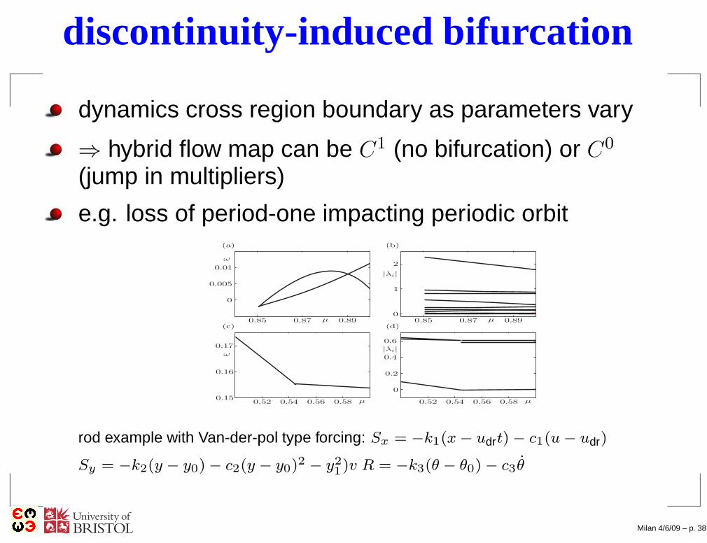
discontinuity-induced bifurcation
dynamics cross region boundary as parameters vary
⇒ hybrid flow map can be C1 (no bifurcation) or C0
(jump in multipliers)
e.g. loss of period-one impacting periodic orbit
0:01
0:005
0
!
0:85 0:87 0:89¹ 0:85 0:87 0:89¹0
1
2
j¸ij
0:17
0:16
0:150:52 0:54 0:56 0:58 ¹
!
0:52 0:54 0:56 0:58 ¹
0
0:2
0:4
0:6
j¸ij
(a) (b)
(c) (d)
rod example with Van-der-pol type forcing: Sx = −k1(x − udrt) − c1(u − udr)
Sy = −k2(y − y0) − c2(y − y0)2 − y21)v R = −k3(θ − θ0) − c3θ
Milan 4/6/09 – p. 38
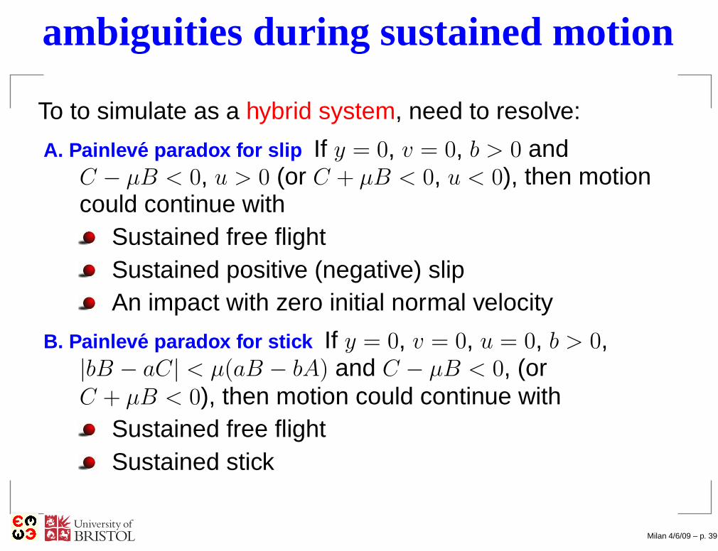
ambiguities during sustained motion
To to simulate as a hybrid system, need to resolve:
A. Painlev e paradox for slip If y = 0, v = 0, b > 0 andC − µB < 0, u > 0 (or C + µB < 0, u < 0), then motioncould continue with
Sustained free flightSustained positive (negative) slipAn impact with zero initial normal velocity
B. Painlev e paradox for stick If y = 0, v = 0, u = 0, b > 0,|bB − aC| < µ(aB − bA) and C − µB < 0, (orC + µB < 0), then motion could continue with
Sustained free flightSustained stick
Milan 4/6/09 – p. 39
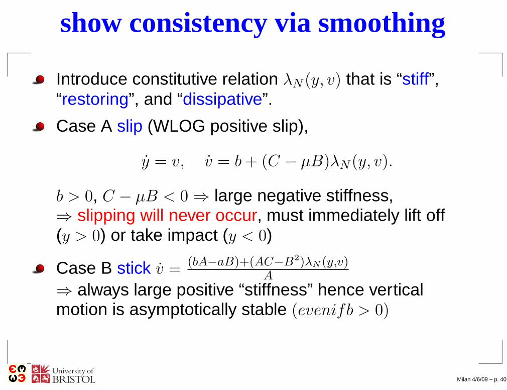
show consistency via smoothing
Introduce constitutive relation λN (y, v) that is “stiff”,“restoring”, and “dissipative”.
Case A slip (WLOG positive slip),
y = v, v = b + (C − µB)λN (y, v).
b > 0, C − µB < 0 ⇒ large negative stiffness,⇒ slipping will never occur, must immediately lift off(y > 0) or take impact (y < 0)
Case B stick v = (bA−aB)+(AC−B2)λN (y,v)A
⇒ always large positive “stiffness” hence verticalmotion is asymptotically stable (evenifb > 0)
Milan 4/6/09 – p. 40
ambiguities at mode transitions
Sustained motion is consistent BUT what about transitions
Case a. approach to the Painlevé boundary(C − µB = 0) during (positive) slip.
previous analysis shows: can’t actually reachC − µB = 0, so what happens instead?
Case b. transitions into stick or chatter
Def: chattering (also known as zeno-ness) isaccumulation of impacts. No contradiction if accumulatein forwards time. But can get reverse chatter.
Milan 4/6/09 – p. 41
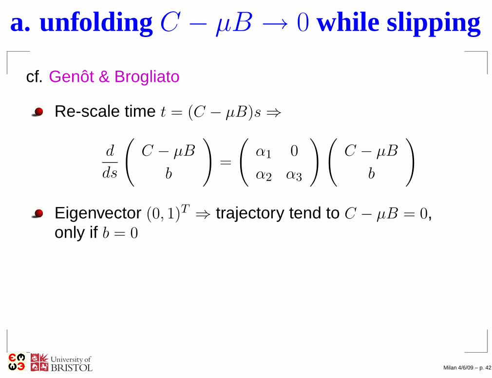
a. unfolding C − µB → 0 while slipping
cf. Genôt & Brogliato
Re-scale time t = (C − µB)s ⇒
d
ds
(
C − µB
b
)
=
(
α1 0
α2 α3
)(
C − µB
b
)
Eigenvector (0, 1)T ⇒ trajectory tend to C − µB = 0,only if b = 0
Milan 4/6/09 – p. 42

approaching the singular point
C ¡ ¹B
b
C ¡ ¹B
b
C ¡ ¹B
b
C ¡ ¹B
b
C ¡ ¹B
b
C ¡ ¹B
b
C ¡ ¹B
b
C ¡ ¹B
b
C ¡ ¹B
b
C ¡ ¹B
b
C ¡ ¹B
b
C ¡ ¹B
b
®2 < 0
®3 > ®1 > 0
®1 > ®3 > 0
®2 > 0 ®2 > 0
®1 > 0 > ®3
®3 > 0 > ®1
®2 < 0
0 > ®1 > ®3
®2 > 0
0 > ®3 > ®1
®2 < 0
®2 < 0
®1 > 0 > ®3
®2 < 0
0 > ®1 > ®3
®2 < 0
®1 > ®3 > 0
®2 > 0
®3 > ®1 > 0
®2 > 0
®3 > 0 > ®1
®2 > 0
0 > ®3 > ®1
Milan 4/6/09 – p. 43
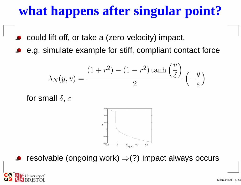
what happens after singular point?
could lift off, or take a (zero-velocity) impact.
e.g. simulate example for stiff, compliant contact force
λN (y, v) =(1 + r2) − (1 − r2) tanh
(v
δ
)
2
(
−y
ε
)
for small δ, ε
−0.1 0 0.1 0.2 0.3−0.4
−0.2
0
0.2
0.4
0.6
C−µ B
b
resolvable (ongoing work) ⇒(?) impact always occurs
Milan 4/6/09 – p. 44
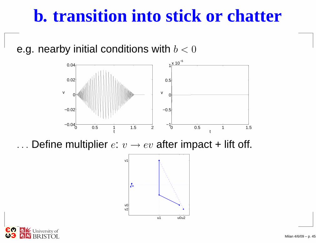
b. transition into stick or chatter
e.g. nearby initial conditions with b < 0
0 0.5 1 1.5 2−0.04
−0.02
0
0.02
0.04
t
v
0 0.5 1 1.5−1
−0.5
0
0.5
1x 10⁻⁶
t
v
. . . Define multiplier e: v → ev after impact + lift off.
u1 u0u2
v2v0
v1
Milan 4/6/09 – p. 45
analysis of chatter
Find parameter regions in which e > 1 (reverse chatter)despite r < 1 - even in the “non-Painlevé” case
Milan 4/6/09 – p. 46
analysis of chatter
Find parameter regions in which e > 1 (reverse chatter)despite r < 1 - even in the “non-Painlevé” case
then we would have “infinite” non-uniqueness inforwards time -:(
Milan 4/6/09 – p. 46

analysis of chatter
Find parameter regions in which e > 1 (reverse chatter)despite r < 1 - even in the “non-Painlevé” case
then we would have “infinite” non-uniqueness inforwards time -:(
but can such transitions occur?
Milan 4/6/09 – p. 46
analysis of chatter
Find parameter regions in which e > 1 (reverse chatter)despite r < 1 - even in the “non-Painlevé” case
then we would have “infinite” non-uniqueness inforwards time -:(
but can such transitions occur?
analysis of smoothed “stiff” systems suggest yes . . .
Milan 4/6/09 – p. 46

analysis of chatter
Find parameter regions in which e > 1 (reverse chatter)despite r < 1 - even in the “non-Painlevé” case
then we would have “infinite” non-uniqueness inforwards time -:(
but can such transitions occur?
analysis of smoothed “stiff” systems suggest yes . . .
it depends how you take the smoothing -:(
ongoing work . . .
Milan 4/6/09 – p. 46

6. Conclusion
used piecewise-smooth as formalism.
Milan 4/6/09 – p. 47
6. Conclusion
used piecewise-smooth as formalism.
⇒ degree of smoothness case by case
Milan 4/6/09 – p. 47
6. Conclusion
used piecewise-smooth as formalism.
⇒ degree of smoothness case by case
⇒ discontinuity induced bifurcationclassification with DMs ⇒ sudden jumps to chaos, etc.
Milan 4/6/09 – p. 47
6. Conclusion
used piecewise-smooth as formalism.
⇒ degree of smoothness case by case
⇒ discontinuity induced bifurcationclassification with DMs ⇒ sudden jumps to chaos, etc.
provides natural explanation of observed behaviour
Milan 4/6/09 – p. 47

6. Conclusion
used piecewise-smooth as formalism.
⇒ degree of smoothness case by case
⇒ discontinuity induced bifurcationclassification with DMs ⇒ sudden jumps to chaos, etc.
provides natural explanation of observed behaviour
much on-going work, e.g.impact + friction Dankowitz, Nordmark & C.catastrophic sliding bifurcations ∼ canards Jeffrey,C. di Bernardo, Shaw, Moehlis
Piecewise-Smooth Dynamical Systems: Theory &Applications diBernardo, Budd, C. & KowalczykSpringer Jan 08. . . + SIAM review Dec 08
Milan 4/6/09 – p. 47