PBL WORKING PAPER 12 MAY 2013 Rocketing rents The magnitude and attenuation of agglomeration economies in the commercial property market1 HANS R.A. KOSTER Department of Spatial Economics, VU University E-mail: h.koster@vu.nl Abstract Rocketing rents in urban areas are likely explained by agglomeration economies. This paper measures the impact of these external economies on commercial property values using unique micro-data on commercial rents and employment. A measure of agglomeration is employed that is continuous over space, avoiding the modifiable areal unit problem. To distinguish agglomeration economies from unobserved endowments and shocks, I use temporal variation in densities and instrumental variables. The spatial extent of agglomeration economies is determined by estimating a spatial bandwidth within the model. The results show that agglomeration economies have a considerable impact on rents: a standard deviation increase in employment density leads to an increase in rents of about 10 percent. The geographical extent of these benefits is about 15 kilometres. The bias of ignoring time-invariant unobserved endowments and unobserved shocks seems to be limited.

JEL classifications: R30, R33 Keywords: commercial buildings; hedonic pricing; agglomeration economies; spatial decay; kernel densities

1 This paper was originally presented as SERC-discussion paper 125 of the London School of Economics (http://www.spatialeconomics.ac.uk/textonly/SERC/publications/download/sercdp0125.pdf), and as Chapter 3 of the PhD thesis Koster, H.R.A. (2013). ´The Internal Structure of Cities: The Economics of Agglomeration, Amenities and Accessibility´. Amsterdam: Rozenberg Publishers.

―2―

1. Introduction The average rent for a unit of office space in New York City is about four times the average rent for a unit of office space in Wichita, Kansas. Also in other high-density cities, such as London, Frankfurt, Milan and Amsterdam, office rents are rocketing. High rents in dense areas are, among other things, caused by agglomeration economies: firms in dense cities seem to be much more productive than in the sparsely populated countryside and are therefore willing to pay higher rents (Glaeser and Gottlieb, 2009; Puga, 2010). Firms aim to locate in dense urban areas because negative crowding effects, such as traffic congestion, high wages and higher crime rates, are more than offset by these positive external economies (Glaeser et al., 2001). Sources of agglomeration economies are proximity to suppliers, access to a thick and well-educated labour market and knowledge spillovers between workers of similar or different firms (Marshall, 1890; Jacobs, 1969; Glaeser et al., 1992; Duranton and Puga, 2002; Ellison et al., 2010).2 So, high rents in contemporary business centres are potentially explained by the many opportunities to interact with other firms: deal-making, relationship adjustment and exchange of tacit knowledge are almost impossible without face-to-face contacts (Storper and Venables, 2004; Amiti and Cameron, 2007). For example, headquarters of manufacturing firms may aim to locate in city centres, because it reduces the costs of interacting with consultants, accountants and lawyers (Davis and Henderson, 2008).

Economists and geographers alike are interested in the magnitude of agglomeration economies for several decades. However, the empirical literature faces a range of challenges in correctly measuring agglomeration economies, which are often proxied by employment density (see Puga, 2010; Combes et al., 2011).3 First, identification of agglomeration economies remains a delicate issue, because employment density is likely correlated to unobserved endowments (Ellison and Glaeser, 1997; 1999; Anas et al., 1999; Bayer and Timmins, 2007; Combes et al., 2011; Ahlfeldt et al., 2012). For example, Ellison and Glaeser (1999) conjecture that at least half of the observed concentration of firms is due to natural advantages. Many studies therefore use long-lagged instruments (e.g. employment density in 1800) or use some imperfect proxy of natural advantages, as to control for these unobserved factors (see e.g. Ciccone and Hall, 1996; Melo et al., 2008; Ellison et al., 2011). The validity of the long-lagged instruments, however, may be questioned.4 Second, the measurement of agglomeration economies is often rather crude. Agglomeration economies are often measured as the density of employment at a city, metropolitan or even state level (Rosenthal and Strange, 2004). As geographical units are arbitrary, this may lead to biased estimates (Briant et al., 2010; Burger et al., 2010). More importantly, aggregate measures 2 In this paper I focus on agglomeration economies that arise between firms in all industries. Often, the literature refers to these agglomeration economies as urbanisation economies or economies of density. 3 Many studies confirm the positive relationship of agglomeration economies using data on firm productivity (e.g. Ciccone and Hall, 1996; Ciccone, 2002; Greenstone et al., 2010; Morikawa, 2011), location choices of start-ups (e.g. Woodward, 1992; Figueiredo et al., 2002; Rosenthal and Strange, 2003; Woodward et al., 2006; Arzaghi and Henderson, 2008), wages (e.g. Glaeser and Maré, 2001; Duranton and Monastiriotis, 2002; Amiti and Cameron, 2007; Combes et al., 2008; 2010), and rents (e.g. Eberts and McMillen, 1999; Drennan and Kelly, 2011). 4 It has frequently been argued that long-lagged unobserved endowments are uncorrelated to current endowments, whereas the past agglomeration pattern is strongly correlated to the current agglomeration pattern (see e.g. Ciccone and Hall, 1996). However, given that one observes extreme persistence of location patterns over time, it may well be that unobserved endowments that were important a century ago are still an important determinant of current rents.

―3―

of density make it difficult to determine the geographical extent of agglomeration economies. It is therefore not surprising that the geographical scope of agglomeration economies is too a large extent unknown.5 Third, Rosenthal and Strange (2004) argue that high rents, as well as high wages, reflect the presence of agglomeration economies, but very few studies use rents to measure the magnitude of agglomeration economies (Puga, 2010). This is particularly unfortunate because agglomeration effects are thought to capitalise mainly into rents rather than into wages, for example because wages are often determined in collective bargaining agreements, which limits the spatial heterogeneity of wages (Arzaghi and Henderson, 2008; Rusinek and Tojerov, 2011; Simón et al., 2006). Additionally, using rents to measure agglomeration economies is insightful, as rents represent a monetary value, in contrast to for example the number of patents or start-ups. Rents are therefore easier to use in appraisals and local cost benefit analyses, allowing for a comparison between industries, so an analysis using commercial rents is not limited to manufacturing industries (see e.g. Acs et al., 1991; Ellison et al., 2011).

The contribution of this paper is threefold. First, this study uses temporal, rather than geographical, variation in densities to estimate agglomeration economies in the Netherlands.6 To control for unobserved shocks, I use instrumental variables (IV). So, the identification strategy deals with time-invariant unobserved endowments and unobserved shocks.7 Second, a new method to determine the geographical scope of agglomeration economies is proposed. Third, I use micro-data on employment and rents to measure agglomeration economies in the commercial property market.

To be more specific, Section II discusses the (theoretical) relationship between productivity, rents, agglomeration economies and consumption amenities, and then proposes a two-step estimation procedure to investigate the magnitude of agglomeration economies on commercial rents. In the first step, I employ kernel methods to estimate weighted employment densities for each location, given a spatial bandwidth, avoiding the arbitrary choice of spatial units. Using a distance decay function and a spatial bandwidth, employment further away contributes less to the kernel density at a certain location. In the second step I regress the rent per unit of floor space on kernel employment densities, while controlling for a wide range of control variables. Most important, I include postcode fixed effects. As these areas are about equal to a US census block, the unobserved heterogeneity with respect to the economic environment can be completely assumed away (see similarly Van Ommeren and Wentink, 2012).8 An important identification issue is that the spatial detail of the postcode fixed effects mitigates the role of fixed unobservable components, but exacerbates the problem of random shocks: when specific areas receive positive (negative) demand shocks, this will lead to higher (lower) densities and rents, implying a spurious correlation (Ottaviano and Peri, 2010; Duranton et al., 2011). Therefore, in addition to including fixed effects, I employ an instrumental variables approach where I use a ‘shift-

5 Cross-sectional studies find that localisation economies (industry-specific agglomeration economies) tend to be very local and attenuate within 7.5 kilometres. However, these studies usually include spatial fixed effects that may capture some agglomeration economies (see Rosenthal and Strange, 2003). Alternatively, they focus on a small study area, so a larger geographical extent is assumed away (see Arzaghi and Henderson, 2008; Ahlfeldt et al., 2012). 6 To use temporal variation in densities based on micro-data is rare. Drennan and Kelly (2011) use temporal variation but rely on data that are aggregated at the metropolitan level. 7 I rely on information on rents rather than sales prices: prices likely generate downward biased results, as prices are forward looking and may capture expected changes in the environment. 8 The average number of employees per postcode six-digit (PC6) location is about 25.

―4―

share’ instrument, following Bartik (1991) and Moretti (2010), among others. So, it is assumed that in absence of local shocks, industries at all locations grew at the national growth rate. I optimise the spatial bandwidth using a cross-validation procedure.9 This implies that one estimates for each bandwidth a hedonic price function and select the model that minimises the cross-validation score.

Greenstone et al. (2010) compare winning and runner-up locations that compete for attracting large firms. A disadvantage of the current study compared to Greenstone et al. (2010) is that I cannot distinguish between different sources of agglomeration economies, due to data limitations. The advantage of this study is that I deal with unobserved demand shocks. Ahlfeldt et al. (2012) use Berlin’s division and reunification as a source of exogenous variation to separate agglomeration economies from unobserved location fundamentals. An attractive feature of their study is that they are able to estimate structural parameters, based on information on land prices, residential and workplace employment. The advantage of the current paper is that it does not has a quasi-experimental set-up, so it seems more general (see also Bajari et al., 2012). The proposed estimation procedure may therefore be used in different time periods and locations. It also puts more emphasis on the estimation of the spatial extent of agglomeration economies.

Section III discusses a unique nation-wide micro-dataset of the Netherlands with employment of all establishments and their exact locations from 1996 to 2010. The Netherlands is dominated by the dense polycentric city region of the Randstad, but it also has many rural areas in the upper northern, southern and eastern parts. Many areas have experienced substantial changes in employment density in the last decade. I also use another micro-dataset containing 25 thousand rental transactions of offices and industrial buildings in the Netherlands from 1997 to 2011.

In Section IV, I present the main results. It is shown that agglomeration has a strong impact on commercial property values. A standard deviation increase in the (weighted) employment density leads to an increase in rents of about 10 percent. To put it differently, doubling of agglomeration leads to an increase in rents of on average 13.5 percent. The geographical scope of agglomeration economies is found to be about 15 kilometres. In line with Combes et al. (2008) and Melo et al. (2008), I find that the bias introduced by ignoring unobserved endowments is limited. Also, unobserved (time-varying) shocks have limited impact on the estimation results, as IV estimates are not statistically significantly different from OLS estimates with fixed effects. I also present other important findings. First, agglomeration economies are an important determinant of rents in the office market, but there is no effect found on rents of industrial space. Second, although the current paper focuses on the economies of density, so urbanisation economies (see Hoover, 1936; 1937), I do not find that localisation economies, so industry-specific agglomeration advantages, capitalise into rents of commercial properties. Third, I do not find evidence that the effect of agglomeration is significantly different between industries. Fourth, it is found that an increase in agglomeration has a stronger effect in urbanised areas.

The results are shown to be robust in Section V, wherein I use other instruments, investigate the decay of agglomeration in more detail and try a plethora of alternative specifications. I also show that the effect of agglomeration is very similar in the housing market, as suggested by the theoretical framework. Section VI concludes. 9 This procedure is standard in nonparametric applications and in the determination of the bandwidth in regression-discontinuity designs, but has not been used in the context of the measurement of agglomeration economies.

―5―

2. Theoretical framework and estimation 2.1 Productivity and rents When agglomeration economies have a positive impact on productivity, one expects to observe higher rents in places where densities are higher. To show this, let us assume that 𝜋𝑗𝑡 is the profit per unit of commercial space of a typical firm in rental property 𝑗 at time 𝑡. Let Γ(𝑛𝑗𝑡) denote some function of employment of firms in all other properties. 𝑛𝑗𝑡 is the spatially weighted employment in the neighbourhood or city. Λ(ℓ𝑗𝑡 , 𝑧𝑗 ,𝑣𝑗𝑡) is a function of some other input ℓ𝑗𝑡, let’s say labour, time-invariant locational endowments 𝑧𝑗 and time-varying endowments 𝑣𝑗𝑡. For convenience, I assume that Λ(ℓ𝑗𝑡, 𝑧𝑗 ,𝑣𝑗𝑡) = �𝑧𝑗𝑣𝑗𝑡�

𝜂ℓ𝑗𝑡𝛼 and Γ�𝑛𝑗𝑡� = e𝜁𝑛𝑗𝑡.10 The profit per square meter of commercial space is then:

(1) 𝜋𝑗𝑡 = �𝑧𝑗𝑣𝑗𝑡�𝜂ℓ𝑗𝑡𝛼e𝜁𝑛𝑗𝑡 − 𝑤𝑗𝑡ℓ𝑗𝑡 − 𝑟𝑗𝑡 ,

where 𝑤𝑗𝑡 is the wage and 𝑟𝑗𝑡 is the rent in rental property 𝑗 at time 𝑡. Given zero profits, it may be shown that the rent per square meter paid by firm in rental property 𝑗 in time period 𝑡 is:

(2) 𝑟𝑗𝑡 = e𝜁

1−𝛼𝑛𝑗𝑡(1 − 𝛼)�𝛼𝑤𝑗𝑡

�

𝛼1−𝛼

�𝑧𝑗𝑣𝑗𝑡�𝜂

1−𝛼.

Note, however, that the wage 𝑤𝑗𝑡 is endogenous and may be a function of house prices and consumption amenities. To show this, assume a worker that gains utility 𝑢𝑡𝑗 in property 𝑗 in time 𝑡 from house size ℎ and a composite commodity 𝑐. For convenience, I assume that workers live where they work and therefore do not incur commuting costs.11 The Cobb-Douglas utility is then 𝑢𝑗𝑡 = Δ�𝑚𝑗𝑡�𝑐𝑗𝑡

𝜙ℎ𝑗𝑡1−𝜙 which is maximised subject to the budget constraint

𝑤𝑗𝑡 = 𝑝𝑗𝑡ℎ𝑗𝑡 − 𝑐𝑗𝑡, where 𝑝𝑗𝑡 is the price for residential space, 𝜙 < 1, and 𝑚𝑗𝑡 is a spatially weighted density of people and let Δ�𝑚𝑗𝑡� = e𝜅𝑚𝑗𝑡. So, when 𝜅 > 0, people prefer to live in dense areas because they may offer (population-induced) amenities. Workers may move to another location where they receive reservation utility 𝑢� and in equilibrium 𝑢𝑗𝑡 = 𝑢�. It may then be shown that the price 𝑝𝑗𝑡 paid per square meter of housing at 𝑗 in time period 𝑡 is:

(3) 𝑝𝑗𝑡 = 𝜙𝜙

1−𝜙e𝜅

1−𝜙𝑚𝑗𝑡(1 − 𝜙) �𝑤𝑗𝑡𝑢��

11−𝜙.

The only wage that is consistent with zero commuting costs is the wage that just equates the bid rents of firms and workers for space at a certain location 𝑗 (see Lucas and Rossi-Hansberg, 2002). This is given by:

(4) 𝑤𝑗𝑡∗ = 𝐾𝑗e1−𝜙1−𝛼𝜙𝜁𝑛𝑗𝑡e

𝛼−11−𝛼𝜙𝜅𝑚𝑗𝑡�𝑧𝑗𝑣𝑗𝑡�

𝜂(1−𝜙)1−𝛼𝜙 ,

where 𝐾𝑗 = �𝜙𝜙(1 − 𝛼)�(1−𝛼)(𝜙−1)

1−𝛼𝜙 𝑢�1−𝛼1−𝛼𝜙𝛼

𝛼(1−𝜙)1−𝛼𝜙 . So, given that 𝜁 > 0 and 𝜅 > 0, wages are higher in

dense areas because of productivity advantages, whereas wages tend to be lower in areas with consumption amenities. When one inserts 𝑤𝑗𝑡∗ into (2) and (3) one has:

10 I pay some attention in the robustness analysis (Section V.E) to functional form assumptions. 11 The assumption of zero commuting costs is harmless if wage is assumed to be constant across the city. The same implications will follow when I assume that workers have to commute to work (see similarly Ottaviano and Peri, 2006). The wage then equates the bid rents of firms and workers for space at the boundary of a central business district.

―6―

(5) 𝑟𝑗𝑡 = 𝑝𝑗𝑡 = e𝜁𝑛𝑗𝑡1−𝛼𝜙e

𝛼𝜅𝑚𝑗𝑡1−𝛼𝜙 (1 − 𝛼)�

𝛼𝐾𝑗�

𝛼1−𝛼

�𝑧𝑗𝑣𝑗𝑡�𝜂

1−𝛼𝜙.

When the above equation is simplified and written in logs:

(6) log 𝑟𝑗𝑡 = 𝛽𝑛𝑗𝑡 + 𝛾𝑚𝑗𝑡 + 𝜆𝑗 + 𝜉𝑗𝑡 ,

Equation (6) is a reduced form equation, so so the coefficient 𝛽 must be interpreted as the marginal effect on productivity, rather than on absolute levels of profits. It holds that 𝛽 = 𝜁 (1 − 𝛼𝜙)⁄ , 𝛾 = 𝜅𝛼 (1 − 𝛼𝜙)⁄ , 𝜆𝑗 = 𝜂 log 𝑧𝑗 (1 − 𝛼𝜙)⁄ and 𝜉𝑗𝑡 = 𝜂 log 𝑣𝑗𝑡 (1 − 𝛼𝜙)⁄ , so 𝜁, 𝜅 and 𝜂 are only identified given a normalisation assumption on 𝛼 and 𝜙. Because 𝛼 < 1 and 𝜙 < 1, 𝛽 is larger than the structural parameter 𝜁. I assume that 𝛽 is time-invariant, an assumption which is tested in the robustness analysis, Section V.E.

Throughout this study, I refer to employment agglomeration 𝑛𝑗𝑡 as agglomeration and to population agglomeration 𝑚𝑗𝑡 as population density. To distinguish agglomeration economies from time-invariant unobserved endowments 𝑧𝑗 I include location fixed effects. Controlling for time-invariant unobserved endowments is potentially important, because rivers and natural resources may attract firms. For example, the port of Rotterdam likely attracts firms, while this is not necessarily because of agglomeration economies (Glaeser, 2008). Also endowments related to the regulatory framework are highly correlated over time. For example, the city centres of Amsterdam and Utrecht are protected historic districts for many decades. Another concern is that simultaneous changes in density and rents are caused by unobserved shocks, denoted by 𝜉𝑗𝑡, leading to a spurious correlation between density and rents. In Section II.C I will therefore pay attention to the construction of an instrument that should be uncorrelated to local shocks.

It has been argued that urban density also facilitates consumption amenities and may be an important reason for the recent growth of many cities (Glaeser et al., 2001; Glaeser and Gottlieb, 2006; Rappaport, 2008). The estimates of agglomeration economies using commercial rents therefore may provide an overestimate of productivity effects. In the presence of productivity advantages, workers have to be compensated for the higher costs of living (Dekle and Eaton, 1999). Note however that, conditional on house prices, locations that offer amenities also offer lower wages (see Rosenthal and Strange, 2002). To separate agglomeration economies from consumption amenities, I will assume that all population-induced amenities are captured by the population density, following Ahlfeldt et al. (2012). This seems reasonable as locations that become attractive to households command higher prices and are likely to attract more households. Consumption amenities are also captured by (time-varying) control variables at a certain location and location fixed effects.

A third issue is that by including location fixed effects I may identify a short-term effect of agglomeration rather than a long-term effect in a cross-sectional setting, which implies that this may be an underestimate of the total effect of agglomeration economies. However, it will be shown that the effect with and without location fixed effects will lead to results that are very similar.

Another implication of this, probably overly stylised, theoretical framework is that agglomeration should have a similar impact on commercial rents 𝑟𝑗𝑡 and house prices 𝑝𝑗𝑡 because in a mixed city 𝑟𝑗𝑡 = 𝑝𝑗𝑡. There may be many reasons why this equality does not strictly hold (e.g. wages 𝑤𝑗𝑡 are not constant across the city, adjustment effects in the housing market, land use planning), but if 𝛽 is similar for the housing market it provides

―7―

additional evidence for the importance of agglomeration economies. I test for agglomeration effects in the housing market in Section V.D. 2.2 A two-step estimation procedure The procedure to estimate equation (6) consists of two steps. First, kernel density functions of employment are estimated, including a spatial bandwidth. In the second step, these kernel densities are inserted into a hedonic price function. The spatial bandwidth is optimised using by repeating these two steps and minimising a cross-validation procedure.

To verify the impact of agglomeration, usually aggregate measures at the county, region, or state level are used. This means that potentially important information is ignored (Duranton and Overman, 2005). It may also lead to an additional bias, especially when the dependent variable is measured in a disaggregate way (as in this paper), while the explanatory variables are not (Briant et al., 2010). In the first step, I therefore use kernel densities that exploit the continuous nature of the data. The employment density for a rental property 𝑗 in period 𝑡 is estimated as:

(7) 𝑛𝑗𝑡(𝛿) = �ℓ𝑘𝑡Ω�𝑑𝑗𝑘,𝛿�𝐾

𝑘=1

,

where ℓ𝑘𝑡 is the employment in another rental property 𝑘 in time 𝑡, where 𝑘 = 1, … ,𝐾, Ω( ∙ ) is some function of 𝛿, which denotes a distance bandwidth, and 𝑑𝑗𝑘 denoting the Euclidian distance between 𝑗 and 𝑘.12 I assume that Ω( ∙ ) is a tricube weighting function, which is often used in spatial applications (McMillen, 2010):

(8) Ω�𝑑𝑗𝑘,𝛿� = �1 − �𝑑𝑗𝑘𝛿�3

�3

𝐼�𝑑𝑗𝑘 < 𝛿�,

where 𝐼( ∙ ) is an indicator function that equals one when the condition is true. As 𝑑𝑗𝑘 will be measured in kilometres, the bandwidth 𝛿 has a clear interpretation. For 𝑑𝑗𝑘 > 𝛿 agglomeration effects are assumed to be zero, so 𝛿 denotes the geographical range of agglomeration economies in kilometres. In contrast to Rosenthal and Strange (2003; 2008) and Arzaghi and Henderson (2008), I estimate smooth density functions instead of using dummies for different distance intervals. The advantage of the current approach is that it is more efficient, because I impose that weights decline in distance. I also avoid arbitrariness in the choice of distance intervals and the model estimates only one coefficient related to agglomeration (instead of one per distance band), which facilitates interpretation. Also, an instrumental variables approach is easier to implement because only one instrument is needed, rather than an instrument for each distance interval. A disadvantage of this approach is that the choice of the kernel function Ω( ∙ ) is arbitrary. I therefore test for alternative kernel functions. Because all kernel functions share the (obvious) feature of declining weights in distance, I show that the estimates are insensitive to the choice of kernel function (see similarly McMillen, 2010; McMillen and Redfearn, 2010). Moreover, I test the functional form of the decay function using distance interval dummies and I show that the tricube weighting function is not rejected (see Section V.C). In contrast, the choice of the bandwidth 𝛿 seems to be more important in the current setting.

12 I use Euclidian distance rather than network travel time because I do not have detailed data on the network. This does not seem to be a problem in the Netherlands, as the correlation between network travel time and Euclidian distance is 0.95.

―8―

In the second step I aim to verify the monetary effect of agglomeration economies. A standard hedonic price approach is employed, which implies that the rent a typical firm is willing to pay for a square meter in rental property 𝑗 at time 𝑡 is regressed on 𝑛𝑗𝑡 and controls, conditional on the choice of the spatial bandwidth 𝛿. Based on equation (6), I then estimate:13

(9) log 𝑟𝑗𝑡 = 𝛽𝑛𝑗𝑡(𝛿) + 𝛾𝑚𝑗𝑡(𝜔) + 𝑏𝑗𝑡′ 𝜃 + 𝜆𝑗 + 𝜏𝑡 + 𝜖𝑗𝑡,

where 𝛽, 𝛾, 𝜃 are parameters to be estimated, 𝜔 is a bandwidth related to population density (the exact definition of 𝑚𝑗𝑡(𝜔) is given in Section III.B), 𝑏𝑗𝑡 are building and location attributes that change over time (such as distance to new stations, land use), 𝜆𝑗 is a location fixed effect, 𝜏𝑡 is a year fixed effect and 𝜖𝑗𝑡 denotes the error term, which is assumed to be independently and identically distributed across firms.14 As argued by Bayer and Timmins (2007), among others, location decisions alone are insufficient in distinguishing the potential of local spillovers from those of locational advantages. As a result, any positive effect of agglomeration is likely to be overstated (Ellison and Glaeser, 1999; Bayer and Timmins, 2007). Because I include location fixed effects at a very low level of aggregation, I effectively control for time-invariant natural advantages and location endowments. So, the key identifying assumption is that changes in 𝜖𝑗𝑡 are uncorrelated to changes in 𝑛𝑗𝑡(𝛿). I also will consider the possibility that agglomeration is correlated to unobserved local shocks, by employing an instrumental variables approach (see Section II.C for more details).

Finally, the spatial bandwidth 𝛿 is determined using a cross-validation procedure. Cross-validation is often used in the determination of the smoothing parameter in nonparametric and semiparametric estimation (Cleveland, 1979; Bowman, 1984; Farber and Páez, 2007; McMillen and Redfearn, 2010). Also in regression-discontinuity designs, a cross-validation procedure is frequently employed to determine the bandwidth (Imbens and Lemieux, 2008; Lee and Lemieux, 2010).15 I define the cross-validation criterion as:

(10) 𝐶𝑉(𝛿) =1𝐽��𝑟𝑗𝑡 − �̂�𝑗𝑡(𝛿)�

2𝐽

𝑗=1

,

where 𝑗 = 1, … , 𝐽. The corresponding bandwidth choice is then given by:

(11) {𝛿∗} = arg min𝐶𝑉(𝛿).

Preferably, 𝛿 is defined as a continuous bandwidth. However, estimating kernel densities of employment for a large dataset is computational intensive. To reduce the computational burden, I therefore assume that 𝛿 is an integer between 0 and 50 kilometres. I will show that the latter is not a limiting assumption, as it is found that 𝛿∗ is always much less than 50 kilometres. The cross-validation scores monotonically increase when 𝛿 gets larger (see Appendix B for more details), so it does not make sense to increase this distance range. One 13 Note that when one has exactly two observations per property 𝑗, equation (9) would be identical to a standard difference-in-difference equation. 14 In an ideal setting, 𝜆𝑗 should denote a rental property fixed effect. I do not include fixed effects at the rental property level, but at the PC6 level. As a consequence, 𝑏𝑗𝑡 therefore also contain time-invariant building attributes and attributes related to the rental contract (so, attributes that vary within a PC6 area). In Section V.E, also building fixed effects are included instead of PC6 fixed effects. 15 One may also use other criteria to determine optimal the bandwidth 𝛿. For example, the Akaike Information Criterion (AIC) and the Bayesion Information Criterion (BIC) are often used (see e.g. Hurvich et al., 1998). It may be shown that these criteria will lead to exactly the same results.

―9―

may argue that there is too little temporal variation in densities to identify the distance parameter. Because densities mainly may change at a local level, the estimation procedure may suggest a too low bandwidth. If this is true, the estimates that do not include fixed effects should suggest a substantially higher spatial bandwidth (because identification in the latter case mainly relies on geographical variation in densities). However, in the analysis it is shown that the spatial bandwidth is reasonably robust across different specifications, regardless of the inclusion of fixed effects.16 2.3 A shift-share instrument As emphasised in Section II.A, agglomeration may be correlated to unobserved time-varying variables, implying a spurious correlation between agglomeration and rents. I therefore need an instrument that is correlated to agglomeration but uncorrelated to unobserved local shocks. Following Bartik (1991), Bartik (1994), Ottaviano and Peri (2007), Moretti (2010) and Faggio and Overman (2012), I will therefore use a ‘shift-share’ approach. The instrument uses the initial employment situation and combines that with national employment growth in an industry. More specifically, it is assumed that, in absence of local shocks, each location would have received a share of employment growth that is in proportion to its initial share.17 Conditional on location fixed effects and when the number of employees in an industry is reasonably large, local shocks should not influence the national employment growth in an industry.

More formally, let 𝑁𝑠𝑡 be the total employment in an industry 𝑠 in year 𝑡, where 𝑠 = 1, … , 𝑆, and 𝑡𝐵 the base year. The predicted number of workers ℓ�𝑠𝑘𝑡 in industry 𝑠 in rental property 𝑘 in year 𝑡 is ℓ�𝑠𝑘𝑡 = �𝑁𝑠𝑡 𝑁𝑠𝑡𝐵⁄ �ℓ𝑠𝑘𝑡𝐵. As an instrument for agglomeration 𝑛𝑗𝑡 I use:

(12) 𝑛�𝑗𝑡(𝛿) = ��ℓ�𝑠𝑘𝑡

𝑆

𝑠=1

Ω�𝑑𝑗𝑘,𝛿�𝐾

𝑘=1

.

So, I re-estimate equation (9) with the predicted kernel employment density 𝑛�𝑗𝑡(𝛿) as an instrument for agglomeration 𝑛𝑗𝑡(𝛿) in a specific year, using the predicted number of workers ℓ�𝑠𝑘𝑡 in a specific industry 𝑠. 3. Data 3.1 LISA-data I use two unique micro-datasets. The first is the LISA employment register. These data provide information on the exact location (geocoded at the address level), the number of employees and information on a five-digit SBI level of all establishments with positive

16 In principle, it is possible to bootstrap this whole procedure to get an estimate for the standard error of 𝛿. However, as in most nonparametric applications, I will not estimate the standard error of 𝛿 to keep the estimation procedure computationally tractable. This implies that I may have a small underestimate of the standard error of 𝛽. However, I will cluster standard errors at the postcode location and show in Appendix B that the variation of 𝛽 across different values of 𝛿 is limited 17 When the number of employees in an industry is very small, local shocks may be correlated to the national employment growth of an industry. This is only an issue when the total employment of a sector changes due to local shocks, i.e. when local shocks induce start-ups or exits. Nevertheless, in almost all cases the total number of employees is large (as an illustration, the average size of an SBI two-digit industry was 72,235 employees in 1996). Also, in the robustness analysis (Section V) it is shown that the results are insensitive to the detail of sectoral classification. Other instruments are also used.

―10―

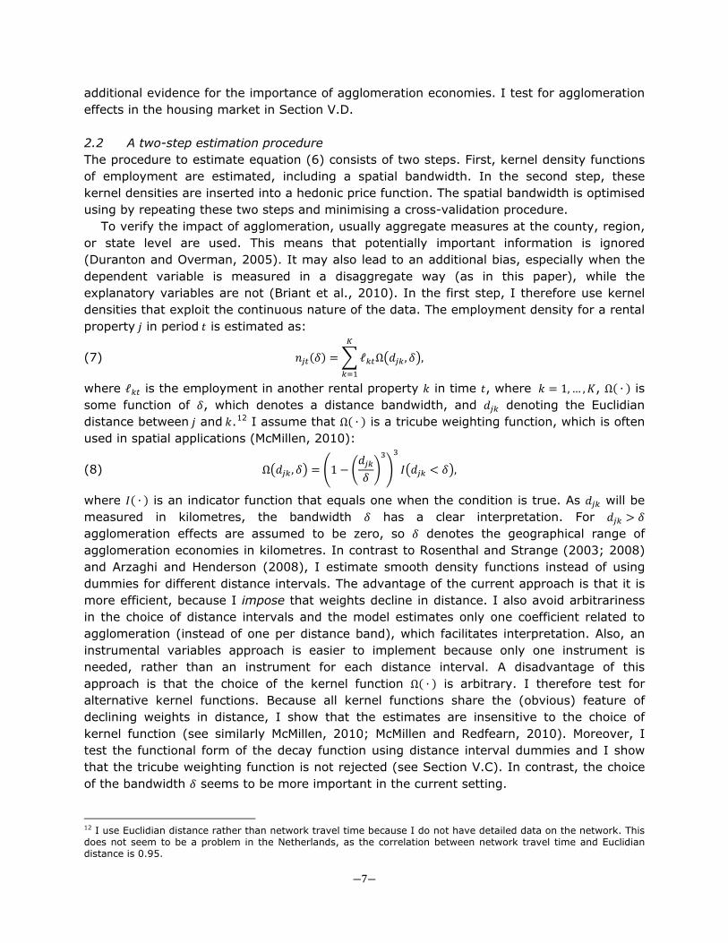
employment in the Netherlands between 1996 and 2010.18 See Van Oort (2004) for a detailed description of these data. The total number of jobs in 1996 was about 6.14 million in 1996 and rose to 7.19 million jobs in 2010 (see Figure 1A). Likely because of the economic crisis, employment growth has slowed down the last decade and total employment even slightly decreases in the last year. In contrast, the number of establishments has increased from 0.66 million in 1996 to 1.11 million in 2010 and is still steadily increasing. As a result, the average firm size is strongly decreasing from 2001 onwards.

Looking at a more disaggregate level, employment growth figures are quite different, which is essential for the identification strategy. For example, the so-called South-Axis in Amsterdam experienced a more than average employment growth. This is the major upcoming business centre in the Netherlands hosting many corporate head offices. On the other hand, another major business centre in the centre of Rotterdam (Weena) showed negative employment growth the last decade. Indeed, some large law firms have recently moved to the South-Axis, likely because of proximity to internationally operating clients and the presence of strong agglomeration economies (see Jacobs et al., 2013).

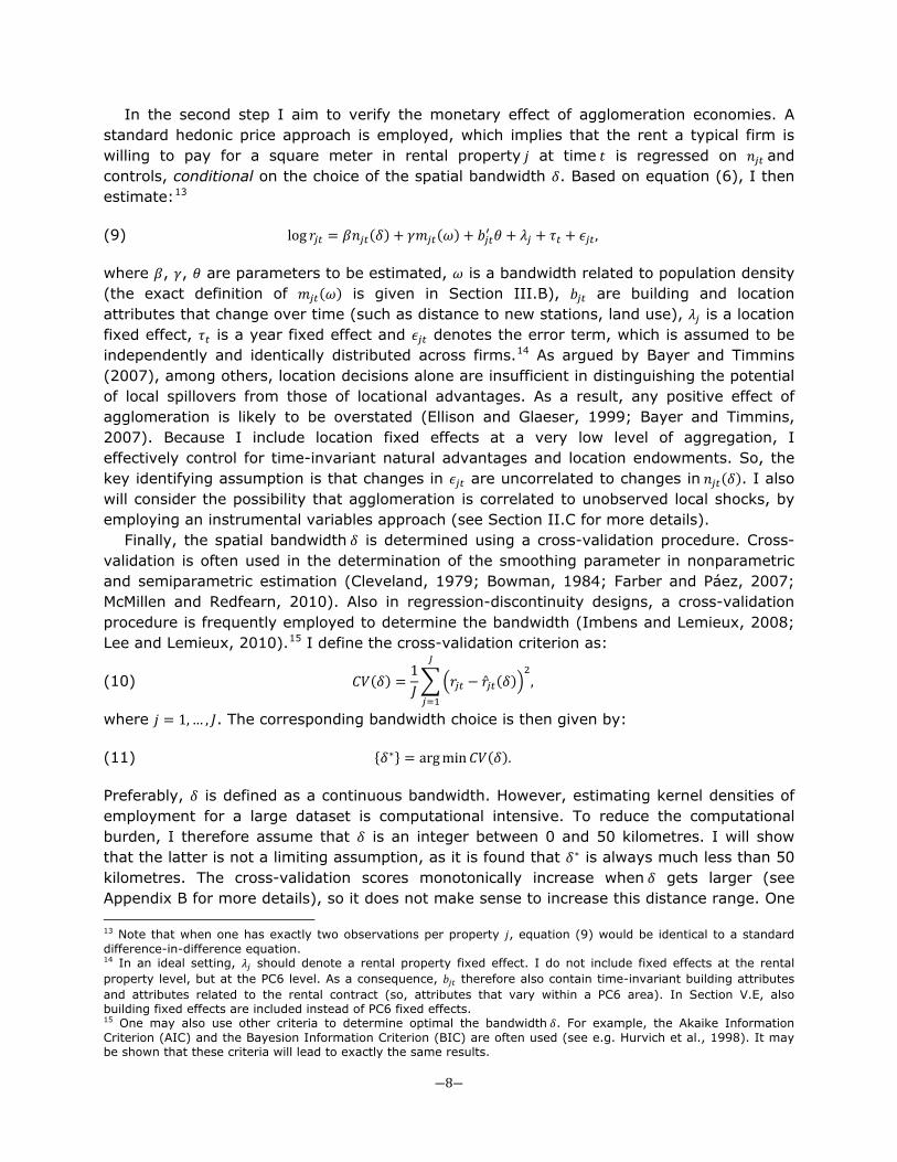
In Figure 2A I map the spatial distribution of employment. All major employment concentrations are part of the so-called Randstad (which is formed by the cities of Amsterdam, Utrecht, The Hague and Rotterdam). It may be shown that in the absolute number of jobs, the Randstad is also the region where most employment growth takes place. There is however a substantial difference between the northern part of the Randstad, which hosts the most important headquarters, business services and ICT firms operating at a supra-regional level, and the southern part of the Randstad, where many logistics and manufacturing activities are located (because of the presence of the port of Rotterdam, which is the largest in Europe). In line with Figure 1B growth rates in the latter part tend to hamper because of the presence of declining industries, whereas Amsterdam and especially some areas nearby Amsterdam tend to experience relatively high growth rates (see Figure 2B).

(A) (B)

FIGURE 1 ― DUTCH EMPLOYMENT FIGURES

18 This classification is comparable to the SIC (Standard Industrial Classification) and NACE (Nomenclature statistique des Activites dans la Communaute Europeenne).

7

8

9

10

6.000

6.500

7.000

7.500

8.000

8.500

9.000

1995 2000 2005 2010

Ave

rag

e Fi

rm S

ize

Emp

loym

ent

(×1

00

0)

Year

Total employmentAverage Firm Size

90

115

140

165

1995 2000 2005 2010

Emp

loym

ent

Ind

ex

(1

99

6 =

10

0)

Year

Total EmploymentAmsterdam - South-axisRotterdam - Weena

―11―

(A) (B)

FIGURE 2 ― SPATIAL DISTRIBUTION AND GROWTH RATES OF DUTCH EMPLOYMENT Notes: In Figure 2A, I calculate for 2010 employment densities. For presentational purposes, I estimate equation (7) for centroids of all four-digit postcode areas (PC4) instead of postcode six-digit areas (a PC4 area is about equal to a census tract in the United States). I set the bandwidth 𝛿 to 15 kilometres. It will be shown in Section IV that this is a reasonable value. In Figure 2B, I calculate the compound annual growth rate using the estimated PC4 employment densities in 1996 and 2010.

3.2 Commercial property data The second dataset that is used is a dataset provided by Strabo, a consultancy firm that gathers and analyses commercial property data. It consists of transactions of commercial office properties, provided by real estate agents between 1997 and 2011.19 The property dataset contains information on the transacted or agreed rent, rental property attributes, such as a geocoded address, size (gross floor area in square meters), and whether the building is newly constructed or renovated.20 Also the share of office and industrial space is included in the dataset, as well as some information on the contract (such as sale-and-lease-back, turnkey properties).21 The dataset also provides information on the broadly-defined industry of the tenant for about 90 percent of the observations.22 After selections, I have 24,086 transactions, of which about 70 percent are transactions related to office space.

19 For the latter year, I only have information for the first two months. 20 I also have information on sales prices. The main reason that I do not use this information in the current paper is because of the limited number of observations (about 10 percent of the number of rent transactions). In the office market it is uncommon that users own properties. Further, renting firms are generally more mobile than owning firms, leading to more transactions. 21 I exclude transactions with missing data on either the price or the size of the rental price, yearly rents per square meter lower than € 20 or higher than € 700 and rental properties that are less than 25 square meters. These selections do not influence the results. 22 Firms are divided in 13 industries: manufacturing, construction, logistics, wholesale, retail, consumer services, hospitality industry, education and healthcare, government, ICT, financial services, business services and other firms. In Table A2, Appendix A, it is shown which SBI codes are part of these broadly-defined industries.

―12―

The rental property dataset is matched to data from the Administration of Buildings and Addresses, which provides the exact location, construction year and energy label (if it has one) for all buildings in the Netherlands. I also define whether the building is multitenant (when it hosts multiple rental properties) and whether it hosts multiple uses (e.g. office, restaurant, shop). Using the Listed Building Register, I include a dummy whether the building is listed. The property dataset is merged with a detailed land use data from Statistics Netherlands for 1996, 2000, 2003, 2006 and 2008. I match each transaction year to the nearest preceding year of the land use data. This may lead to some bias, but as the average time difference between transactions in the same postcode six-digit location (PC6) is about 2.5 year, I expect that the bias is limited. The latter data enable me to calculate the distance to the nearest hectare of commercial land, open space, water, major roads and railways. I also include the land use of the actual location (industrial, commercial, residential or other) and the distance to the nearest station.

Population density (𝑚𝑗𝑡) at a postcode four-digit level is also included as a control variable. To calculate the (weighted) population density, I first assume that population is uniformly distributed over all PC6 locations in a PC4 area. Population density is then measured as 𝑚𝑗𝑡 = ∑ 𝑎𝑘𝑡Ω�𝑑𝑗𝑘,𝜔�𝐾

𝑘=1 , where 𝑎𝑘𝑡 is the number of people at a certain location 𝑘 and 𝜔 is a fixed bandwidth. So, 𝑚𝑗𝑡 is a ‘lumpy’ approximation of the continuous kernel density of population density. To save computation time, I will provisionally assume that 𝜔 = 2.5; when population density reflects the presence of amenities, the benefits are expected to be very local (see Koster and Rouwendal, 2012). In the sensitivity analysis (Section V.E) I will jointly optimise 𝛿 and 𝜔 and show that the results of agglomeration are almost unaffected.

Using the Listed Building Register I determine whether the rental property is in an area that is assigned as a historic district, or which is in the process of becoming a designated historic district. As I include spatial fixed effects at the PC6 location, I identify the coefficients related to land use and population density based on changes. The coefficient of stations is identified using new station openings. It is also important to note that all variables related to the environment (including agglomeration) are referring to the year preceding the transaction to avoid simultaneity bias, but also because location choices likely imply a thorough preliminary study of local markets in a previous period (Greenstone et al., 2010; Hilber and Voicu, 2010).23

In Table A1 in Appendix A descriptive statistics are presented. The average rent is € 105 per square meter and the standard deviation is about € 54 per square meter. The most expensive office space can be found in and close to Amsterdam with average rents of about € 180 per square meter, whereas office space in the upper north, east and south of the Netherlands can be as low as € 50 per square meter, so there is substantial spatial variation in the rents for office space. For industrial buildings, the variation is less with average prices ranging from € 30 to € 100 per square meter. Most rental properties are either in a commercial area or at an industrial site, but still about 20 percent of the observations are in

23 One may argue that kernel densities of employment are biased if the firm’s own employment is included in the kernel density. Because the kernel densities are estimated in the year that precedes the transaction and because most observations are movers or start-ups, this bias is likely to be small. Further, I identify agglomeration based on changes in densities. Firms that stay do therefore not contribute to identification of the agglomeration effect. Nevertheless, in the robustness analysis (Section V.E), it is shown that the effect of agglomeration is very similar when I exclude firms that have prolonged their contracts (so, the latter firms are not movers or start-ups).

―13―

(A) (B) FIGURE 3 ― AGGLOMERATION AND RENTS

Notes: It is assumed that the bandwidth 𝛿 = 15. In 3B, I plot the average annual change in rents in a PC6 area 𝑗 in year 𝑡, �𝑟𝑗𝑡1 − 𝑟𝑗𝑡0� (𝑡1 − 𝑡0)⁄ , against the average annual change in agglomeration 𝑛𝑗𝑡, �𝑛𝑗𝑡1 − 𝑛𝑗𝑡0� (𝑡1 − 𝑡0)⁄ , in a PC6 area.

a residential area. The average size of the rental property is 1,173 square meters, which is almost twice the median size (630 square meter). Almost 80 percent of the transactions are in postcodes with more than one observation, which seems sufficiently high to use temporal variation in explanatory variables as a source of identification. In Figure 3A, I plot agglomeration (using 𝛿 = 15) against rents. None of the controls are included, so these results are suggestive, at best. Nevertheless, this univariate regression suggests that a standard deviation increase in agglomeration increases rents with on average 32 percent. Figure 3B plots the annual changes in rents against annual changes in agglomeration. This suggests that rents increase with 45 percent when agglomeration increases with one standard deviation. 4. Results 4.1 Baseline regressions Table 1 presents the baseline results of the effects of agglomeration 𝑛𝑗𝑡 on rents. I first run standard OLS and instrumental variables regressions without PC6 fixed effects 𝜆𝑗. Specification (1) suggests that there is a considerable effect of agglomeration: one standard deviation increase in (weighted) employment density 𝑛𝑗𝑡 may lead to an increase in rents of 13.1 percent. Using the cross-validation procedure, it appears that the geographical range of agglomeration economies is 17 kilometres.24

24 When I include municipality fixed effects, the estimate of agglomeration is 0.117, which is similar to Specification (1). This suggests that, given the explanatory variables included, municipality fixed effects do not capture unobserved endowments.

0

100

200

300

400

500

-1,5 -0,5 0,5 1,5 2,5 3,5

Ren

ts p

er m

² (i

n €

)

Agglomeration (in std. dev.)

-100

-50

0

50

100

-0,1 0,0 0,1 0,2 0,3

An

nu

al c

han

ge

in

ren

ts (

in €

)

Annual change in agglomeration (in std. dev.)

―14―

TABLE 1 ― REGRESSION RESULTS ON THE IMPACT OF AGGLOMERATION (Dependent variable: the logarithm of commercial rent per square meter)

(1) (2) (3) (4) OLS IV FE IV – FE Agglomeration, 𝑛𝑗𝑡 0.133 (0.004) *** 0.115 (0.021) *** 0.099 (0.031) *** 0.120 (0.035) *** Population density, 𝑚𝑗𝑡 0.022 (0.005) *** 0.036 (0.013) *** 0.012 (0.039) 0.014 (0.038) Land use – residential -0.019 (0.011) * -0.019 (0.011) * 0.048 (0.016) *** 0.048 (0.016) *** Land use – industrial site -0.121 (0.011) *** -0.116 (0.012) *** -0.010 (0.014) -0.011 (0.014) Land use – other -0.034 (0.014) ** -0.030 (0.015) ** 0.034 (0.018) * 0.033 (0.018) * Distance to industrial land (km) -0.048 (0.024) ** -0.044 (0.026) * -0.109 (0.031) *** -0.110 (0.031) *** Distance to major road (km) -0.100 (0.030) *** -0.082 (0.034) ** -0.048 (0.061) -0.044 (0.061) Distance to railway (km) 0.006 (0.002) *** 0.005 (0.002) ** -0.007 (0.007) -0.007 (0.007) Distance to station (km) -0.016 (0.002) *** -0.015 (0.002) *** 0.006 (0.012) 0.006 (0.012) Distance to open space (km) -0.086 (0.018) *** -0.088 (0.018) *** -0.086 (0.033) *** -0.086 (0.033) *** Distance to water (km) -0.027 (0.006) *** -0.030 (0.008) *** -0.034 (0.021) -0.034 (0.021) Historic district – in process 0.054 (0.033) * 0.053 (0.033) 0.043 (0.033) 0.045 (0.033) Historic district – assigned 0.048 (0.014) *** 0.048 (0.014) *** 0.122 (0.045) *** 0.121 (0.049) *** Green heart 0.060 (0.012) *** 0.046 (0.013) *** 0.023 (0.015) 0.024 (0.015) Size in m² (log) -0.036 (0.004) *** -0.035 (0.004) *** -0.041 (0.004) *** -0.041 (0.004) *** Share industrial space -0.759 (0.009) *** -0.763 (0.010) *** -0.550 (0.013) *** -0.550 (0.013) *** Newly Constructed 0.097 (0.011) *** 0.098 (0.011) *** 0.065 (0.009) *** 0.065 (0.009) *** Renovated 0.094 (0.024) *** 0.097 (0.026) *** 0.052 (0.014) *** 0.052 (0.014) *** Parking spaces (log) 0.050 (0.005) *** 0.049 (0.005) *** 0.033 (0.004) *** 0.033 (0.004) *** Listed building 0.061 (0.019) *** 0.060 (0.019) *** 0.019 (0.027) 0.018 (0.027) Energy label A 0.027 (0.030) 0.025 (0.030) 0.052 (0.029) * 0.052 (0.029) * Building surface area in m² (log) -0.005 (0.003) * -0.005 (0.004) -0.015 (0.004) *** -0.015 (0.004) *** Building – multitenant 0.034 (0.007) *** 0.033 (0.007) *** 0.002 (0.008) 0.002 (0.008) Building – multiple uses -0.045 (0.008) *** -0.045 (0.008) *** -0.016 (0.010) -0.016 (0.010) Rent – turnkey 0.151 (0.035) *** 0.158 (0.035) *** 0.133 (0.029) *** 0.133 (0.029) *** Rent – sub rent 0.022 (0.015) 0.027 (0.015) * -0.015 (0.012) -0.015 (0.012) Rent – sale and lease back 0.064 (0.024) *** 0.060 (0.025) ** 0.036 (0.029) 0.036 (0.030) Rent – contract prolongation 0.019 (0.012) 0.022 (0.012) * -0.013 (0.009) -0.013 (0.009) Rent – length contract (in years) 0.018 (0.003) *** 0.018 (0.003) *** 0.005 (0.003) 0.005 (0.003) Other control variables (9) Yes Yes Yes Yes Year fixed effects (15) Yes Yes Yes Yes PC6 fixed effects (8,461) No No Yes Yes Spatial bandwidth 𝛿∗ (km) 16 18 13 17 Cross validation score 𝐶𝑉(𝛿∗) 0.07941 0.07940 0.03706 0.03707 R² 0.7329 0.9192 F-Test weak instruments 103.218 3,187.732 Notes: The number of observations is 24,086. Other control variables are parking spaces missing, contract length missing and seven construction decade dummies. In Specification (2), the instruments of agglomeration are the logarithm of municipal population density in 1830 and distance to station in 1870. In Specification (4), the shift-share instrument is used (see equation (12)). First-stage results are presented in Table C2, Appendix C. Standard errors are clustered at the postcode six-digit location. *** Significant at the 0.01 level ** Significant at the 0.05 level * Significant at the 0.10 level

In Specification (2), I estimate an instrumental variables regression. The standard procedure to control for unobserved locational advantages is to use long-lagged instruments. I use the logarithm of municipal population density in 1830. Note that municipalities in 1830 were much smaller and do not overlap with current ones. The Netherlands in 1830 consisted of 1,228 municipalities, whereas nowadays it consists of only 431 municipalities. The instrument’s validity rests on the (debatable) assumption that population density in 1830 is unrelated to current unobserved locational advantages (and therefore productivity of firms), but has a causal effect on the current agglomeration pattern (see also Ciccone and Hall, 1996; Rice et al., 2006; Combes et al., 2008). This instrument is strong as geographical concentration of firms and people are strongly autocorrelated (McMillen and McDonald,

―15―

1998). The second instrument I employ is the distance to the nearest station in 1870. Stations were an important factor that caused agglomeration in the second half of the 19th century (Ciccone and Hall, 1996). Specification (2) shows that the impact of agglomeration is only 1.8 percentage points lower.25 Using the Hausman t-statistic, it appears that the coefficient of agglomeration is not statistically significantly different from the estimate in Specification (1) at the five percent level (the t-statistic is 0.89).26 The spatial bandwidth of agglomeration economies is 18 kilometres. The latter specification may produce an inconsistent estimate of agglomeration if current unobserved endowments are correlated with past unobserved endowments. In Specification (3) I therefore include 8,461 PC6 fixed effects. It is shown that the effect of agglomeration is still substantial and statistically significant.27 One standard deviation increase in agglomeration leads to an increase in rents of 9.9 percent. Alternatively, doubling of agglomeration leads to an increase in rents of on average 13.6 percent. For an area with a median level of agglomeration, this is 9.9 percent. It is important to note that the bandwidth is very similar to the specifications that (mainly) rely on geographical variation in densities as a source of identification. Compared to Specifications (1) and (2), the results of Specification (3) suggest that estimates employing ordinary least squares and instrumental variables are not upward biased. The Hausman t-statistic for the difference with the OLS without fixed effects is 1.11. The difference with the IV estimates without fixed effects is also statistically insignificant (the Hausman t-statistic is 0.69).28

In Specification (4) agglomeration is instrumented with the predicted agglomeration pattern based on the shift-share methodology. The instrument is (very) strong, so most of the changes in employment can be explained by the initial sectoral employment share and national trends. The coefficient of agglomeration suggests that a standard deviation increase in agglomeration leads to an increase in rents of 12 percent, which is slightly higher than the estimate in Specification (3). However, this coefficient is not significantly different from the coefficient in Specification (3) (the Hausman t-statistic is -1.40). One may conclude that unobserved shocks are not strongly correlated to measures of employment density. Because Specification (3) is then more efficient, this is the preferred specification. So, conditional on covariates, time-invariant unobserved endowments and unobserved shocks seem to play a limited role in the market for commercial properties, in line with Combes et al. (2008) and Melo et al. (2008), among others. In accordance with Arzaghi and Henderson (2008), it seems that agglomeration economies mainly capitalise into rents, rather than into wages, as the effect of agglomeration economies on wages is found to be an order of magnitude smaller (typically between two and five percent, see Combes et al. 2008; 2010; and for the Netherlands: Groot et al., 2011). One explanation may be that wage bargaining agreements limit geographical variation in wages and therefore also the possibility of agglomeration economies to capitalise into wages. In contrast, there are no rent-controls in the commercial property market in the Netherlands. Another reason may be that commuting trips, which

25 First-stage results are presented in Appendix C, as well as descriptives of the instruments. 26 The Hausman t-statistic is calculated as 𝑡𝛽� = ��̂�𝑂𝐿𝑆 − �̂�𝐼𝑉� �𝜎𝛽�𝐼𝑉

2 − 𝜎𝛽�𝑂𝐿𝑆2� (see Wooldridge, 2002, pp. 120).

27 In Appendix B it is shown that the cross-validation score is minimised when 𝛿 = 13 (Figure B1). 28 This result only holds because of the large number of relevant control variables. When I exclude all variables except year fixed effects and re-estimate Specifications (2) and (3) the coefficients are respectively 0.241 and 0.103. The Hausman t-statistic is then 5.53.

―16―

capitalise in wages, are only made once a day, while intra-firm trips are made multiple times a day.

It appears that the geographical range of agglomeration economies is about 15 kilometres. That is not to say that there are no interactions over longer distances. For example, input-output relationships between firms are likely to decay slower and are even occurring between firms in different continents. However, these long-distance input-output relationships are unlikely to be a main driver of local rents. Storper and Venables (2004) Amiti and Cameron (2007) and Arzaghi and Henderson (2008) argue that especially an abundant supply of possibilities to engage in face-to-face contacts capitalises into rents, which seems to be in line with the results of the current study. For example, these findings are in accordance with the observation that businesses that offer specialised services to maritime industries are mostly located in Rotterdam, which hosts Europe’s largest port (see Jacobs et al., 2011). Similarly, many large law and accountants firms that offer face-to-face services to corporate headquarters are concentrated in Amsterdam, which hosts the largest concentration of headquarters in the Netherlands (see Jacobs et al., 2012).

Control variables have in general plausible effects on rents. Population density has a positive impact on commercial rents in Specifications (1) and (2). However, when I include PC6 fixed effects, the effect of population density becomes statistically insignificant.29 It is shown that locations further away from commercial land are much cheaper, ranging from 6 to 11 percent per kilometre. Locations near open spaces are also considered as attractive, likely because they offer amenities to workers. I also find a statistically significant positive effect of historic district designation, implying a rent increase ranging from 6 to 12 percent. Further, industrial buildings tend to be cheaper, which is not surprising as office space refers to a much higher quality building, in particular internally, whereas industrial buildings are usually bare. Also newly constructed and renovated buildings tend to be more expensive. The number of available parking spaces is positively related to rents (see similarly Van Ommeren and Wentink, 2010). In line with Eichholtz et al. (2010), energy-efficient buildings tend to be more expensive, although this effect is only marginally significant. 4.2 Other results In this subsection I discuss other relevant results. In particular, one may wonder whether the results differ for offices and industrial buildings, whether there is an effect of localisation (or industry-specific agglomeration economies), whether the importance of agglomeration economies differs between industries and whether the effect of agglomeration is nonlinear. The results are presented in Table 2 and Figures 4 and 5. It may be expected that agglomeration economies are not equally important for firms occupying offices and industrial buildings. Therefore, I estimate separate specifications for these submarkets. Specification (5) only includes rental transactions for which at least half of the rented size refers to office space. It appears that the effect of agglomeration is very similar to the effect found in Specification (3): one standard deviation increase in agglomeration leads to an increase in rents of 10 percent. It is also shown that the spatial

29 One may argue that population density may pick up some effect of agglomeration economies (e.g. external economies related to a thick labour market). Nevertheless, when I exclude population density, the coefficient of agglomeration is almost identical. See Section V.E for more details.

―17―

TABLE 2 ― REGRESSION RESULTS, ALTERNATIVE SPECIFICATIONS (Dependent variable: the logarithm of rent per square meter)

(5) (6) (7) (8) (9)

FE

Offices FE

Industrial Buildings

FE Localisation

FE Industry-

specific effect

FE Nonlinear

effect Agglomeration, 𝑛𝑗𝑡 0.100 -0.079 0.098 (0.033) *** (0.088) (0.031) *** Localisation, 𝑛𝑗𝑡𝑙𝑜𝑐 0.003 (0.002) Agglomeration, 𝑛𝑗𝑡, industry-specific effects (14) No No No Yes No

Agglomeration, 𝑛𝑗𝑡, centile-specific effects (10) No No No No Yes

Control variables included (51) Yes Yes Yes Yes Yes PC6 fixed effects (8,461) Yes Yes Yes Yes Yes Spatial bandwidth 𝛿∗ (km) 11 6 13 14 14 Spatial bandwidth localisation 𝛿𝑙𝑜𝑐∗ (km) 2 Cross-validation score 0.02441 0.04523 0.03706 0.03699 0.03701 R² 0.8612 0.8400 0.9193 0.9195 0.9194 Notes: The number of observations in Specifications (5) and (6) is respectively 15,823 and 8,263. See Table 1.

bandwidth is now slightly lower and 11 kilometres. In Specification (6), I concentrate on industrial buildings. It is shown that the coefficient of agglomeration is statistically insignificant. This is not too surprising as industrial buildings are often located in low-density low-rent areas where agglomeration economies seem to be less important, whereas firms in offices likely rely much more on costly face-to-face contacts.30 The negative point estimate suggests the possibility of a negative effect of employment density. However, the point estimate is very sensitive to the choice of bandwidth, e.g. when 𝛿 = 4, the point estimate is -0.003.

Specification (7) adds a variable that measures the number of employees in the own-industry (or localisation) (see Table A2, Appendix A for the industrial classification).31 It is shown that the coefficient of agglomeration is about the same as in Specification (3) and localisation does not have an effect on rents. Note that the spatial bandwidth of localisation is much lower (2 kilometre) because it is hard to properly estimate a spatial bandwidth when an effect is (almost) absent. It may be that the effect of agglomeration is heterogeneous between firms in different industries. So, agglomeration is interacted with industry dummies (see Specification (8)). It is shown in Figure 4 that the effect of agglomeration is not statistically significantly different across different industries (the F-test is 1.33).32

Specification (9) considers the possibility of a nonlinear effect of agglomeration. Agglomeration 𝑛𝑗𝑡 is therefore interacted with centile dummies. Figure 5 shows the marginal

30 As an illustration, the average (standardised) value of agglomeration for industrial buildings is -0.349, while it is 0.188 for offices for 𝛿 = 13. 31 I estimate localisation densities as 𝑛𝑠𝑗𝑡𝑙𝑜𝑐(𝛿𝑙𝑜𝑐) = ∑ ℓ𝑠𝑘𝑡Ω�𝑑𝑗𝑘 , 𝛿𝑙𝑜𝑐�𝐾

𝑘=1 . For 10 percent of the transactions I do not have data on the industry 𝑠, so I cannot estimate localisation densities. I then include a dummy in the specification when localisation is missing. Excluding these observation will lead to almost identical results. 32 Koster et al. (2013) also found that there is only modest heterogeneity of the agglomeration effect between industries. They show that only retailers and the government are willing to pay substantially more for agglomeration. However, in that paper, also shops are taken into account, which explains the strong preference of retailers for dense areas.

―18―

FIGURE 4 ― HETEROGENEITY IN THE EFFECT OF AGGLOMERATION Notes: The dashed vertical bars denote 95 percent confidence intervals and the horizontal bars denote point estimates for each industry.

FIGURE 5 ― NONLINEAR EFFECT OF AGGLOMERATION

effect of agglomeration for different values of agglomeration. The results suggest that agglomeration benefits are more pronounced in dense areas. For example, in a strongly urbanised area (e.g. Amsterdam or Rotterdam) a standard deviation increase in agglomeration leads to an increase in rents of about 10 percent, whereas on the countryside a standard deviation increase in agglomeration seems to have no impact on rents. For low values of agglomeration, the confidence intervals are relatively wide, so I cannot reject a linear relationship of agglomeration, as the coefficient of Specification (3) almost always falls in the 95 confidence interval.

-0,20

-0,10

0,00

0,10

0,20

Effe

ct o

f ag

glo

mer

atio

n, β

-0,40

-0,30

-0,20

-0,10

0,00

0,10

0,20

0,30

-1,5 -1,0 -0,5 0,0 0,5 1,0 1,5 2,0 2,5 3,0 3,5

Effe

ct o

f ag

glo

mer

atio

n, β

Agglomeration (in std.dev.)

―19―

5. Robustness analysis 5.1 Introduction The robustness analysis focuses on four sets of issues. First, is the regression using a shift-share instrument robust? I will use other instruments and use other approaches to test the correlation of agglomeration to unobserved shocks. Second, is the assumption of a Tricube weighting function for the spatial decay of agglomeration appropriate? Third, does agglomeration impact house prices in a similar way, as is suggested by the theoretical framework? Fourth, is the measure of agglomeration robust to excluding time-varying locational endowments and geographical size of the fixed effects? 5.2 Endogeneity of agglomeration To identify the causal impact of agglomeration on commercial rents, changes in unobserved endowments should be uncorrelated to changes in agglomeration. In this subsection I will investigate whether the results of Specification (4) are robust to other assumptions on how shocks impact the local environment. The results are presented in Table 3. First, in Specification (10), I construct the shift-share instrument on the SBI five-digit level. It may be argued that when industries are reasonably small, the shift-share instrument may be correlated to local shocks. Again, this argument only applies when local shocks impact the total number of employees in an industry, so when local shocks induce start-ups or exits. When I use the most detailed SBI five-digit sectoral classification (the average size of an industry was only 7,782 employees in 1996), one may conjecture that the results are biased and different from the estimates in Specification (4), which relies on a much less detailed sectoral classification. However, it is shown that the results are almost identical to the results of Specification (4), suggesting that my instrument is valid.

One may criticise the use of a shift-share instrument, for example because trends in employment growth may be correlated with initial industrial shares at certain locations. To

TABLE 3 ― REGRESSION RESULTS, AGGLOMERATION AND SHOCKS (Dependent variable: the logarithm of rent per square meter)

(10) (11) (12) (13) (14)

IV – FE SBI five-

digit instrument

FE Municipa-lity

trends

FE NUTS2-year,

coordinates

IV – FE Political

instruments

IV – FE Political

instruments

Agglomeration, 𝑛𝑗𝑡 0.121 0.163 0.162 0.132 0.208 (0.034) *** (0.066) ** (0.040) *** (0.097) (0.147) Control variables included (51) Yes Yes Yes Yes Yes PC6 fixed effects (8,461) Yes Yes Yes Yes Yes Municipality-specific trends (714) No Yes No No No NUTS2-year fixed effects (180) No No Yes No Yes Function of location and year Θ( ∙ ) No No Yes No Yes Spatial bandwidth 𝛿∗ (in km) 17 11 14 10 13 Cross validation score 𝐶𝑉(𝛿) 0.03707 0.03589 0.03649 0.03707 0.03610 R² 0.9241 0.9214 F-Test first-stage 2,816.425 194.023 135.929 Notes: See Table 1. The instrument in Specification (8) is the shift-share instrument (see equation (12)) based on a five-digit SBI level. Instruments in Specification (13) and (14) are the municipal share of voters for socialist parties, the share of voters for liberal parties and the share of voters for Christian parties and the share if these parties have the maximum share. Reference category is the share of voters for local parties. First-stage results are presented in Table B1, Appendix B.

―20―

deal with this criticism, I assume that shocks operate at a municipal scale. For example, some municipality-specific subsidies may attract firms, which lead to higher rents. In Specification (11), I include linear-quadratic time trends for each municipality to control for changes in unobservables. It is shown that the effect of agglomeration is somewhat higher: one standard deviation increase in agglomeration leads to an increase in rents of 16.2 percent, which suggests that the preferred estimate is a lower bound estimate of the effect of agglomeration. However, the Hausman t-statistic does not suggest that the coefficient of agglomeration economies is statistically different from Specification (3) (the t-value is -1.09).

Another way to proceed is to include fixed effects for each NUTS2 area ℎ in each year.33 However, it is likely that there are local unobserved time-varying endowments. It is then assumed that these time-varying unobserved endowments are continuous and smooth over space and not (perfectly) collinear with agglomeration, so that these are captured by a flexible nonparametric function of geographic coordinates and time. I estimate log 𝑟ℎ𝑗𝑡 =𝛽𝑛𝑗ℎ𝑡(𝛿) + 𝛾𝑚𝑗ℎ𝑡 + 𝑏𝑗ℎ𝑡′ 𝜃 + Θℎ(𝑥,𝑦, 𝑡) + 𝜇ℎ𝑡 + 𝜆𝑗 + 𝜏𝑡 + 𝜖𝑗ℎ𝑡 , where Θℎ( ∙ ) is a flexible NUTS2-specific function of the 𝑥-coordinate, the 𝑦-coordinate and year 𝑡, and 𝜇ℎ𝑡 denotes a NUTS2-year fixed effect. It is shown that the coefficient of agglomeration is statistically significantly higher than the preferred estimate, so the initial estimate may be somewhat conservative (the Hausman t-statistic is -2.40).

Specification (13) uses alternative instruments to control for unobserved shocks. Following Duranton et al. (2011), I use political instruments. Using data from the Election Council, I calculate the municipal shares of votes for local parties, liberal (right-wing) parties, socialist (left-wing) parties and Christian parties. Especially socialist parties tend to focus on low unemployment rates and therefore aim to create new jobs. Right-wing liberal parties tend to be more focused on attracting high income households and guarantee high levels of education. As government assistance to individual firms is considered as undesirable, vote shares arguably only impact rents via aggregate changes in agglomeration levels, conditional on control variables (see Duranton et al., 2011 for a similar argument). Municipal elections took place in 1994, 1998, 2002, 2006 and 2010, so there is spatial and temporal variation in vote shares. Specification (13) shows that agglomeration has a positive impact on rents similar to Specification (3), but the effect is not statistically significant.34 Duranton et al. (2011) argue that the validity of the political instruments may be questioned without spatial differencing, because the share of voters for a political party may be correlated with unobserved shocks. I therefore re-estimate Specification (3), but now I include region-year fixed 𝜇ℎ𝑡 effects and a flexible function of location and time Θℎ( ∙ ). Specification (14) shows that the coefficient of agglomeration is now higher (0.208) but is not statistically significantly different from Specification (3) (the Hausman t-value is -0.76)

All in all, the results suggest that agglomeration is not strongly correlated to shocks. The specifications in this subsection suggest a slightly higher coefficient of agglomeration, so the preferred estimate (Specification (3)) seems to be somewhat conservative.

33 A NUTS2 (Nomenclature of Territorial Units for Statistics) area is comparable in size to Metropolitan Statistical Areas (MSAs) in the United States. In the Netherlands, there are 12 NUTS2 regions, usually labelled provinces. The time period of the sample is 15 years, which implies 180 fixed effects. 34 I include vote shares and the vote shares if it is the maximum share. As, in the Netherlands, parties almost always have to form coalitions, it makes sense to include also the maximum vote shares.

―21―

5.3 Spatial attenuation of agglomeration economies As acknowledged earlier, the choice of the kernel function is arbitrary. I will first employ a nonparametric weighting function by including the total employment in 5 kilometres rings around the employment location, following Rosenthal and Stange (2002). Then, I compare the estimates using the Tricube weighting function with a Triangular, an Exponential and an Epanechnikov kernel. Table 4 presents the results.

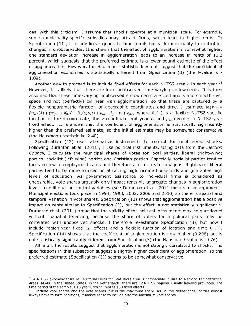
Specification (15) shows that an increase of 113,429 employees within 5 kilometres increases rents with 10.5 percent.35 This effect is almost half when this increase is between 5 and 10 kilometres of the firm location. For distances larger than 10 kilometres, the effect becomes effectively zero. I plot this relationship in Figure 6, together with the spatial attenuation implied by Tricube weighting function, based on Specification (3). It is shown that the Tricube weighting function is always within the 95 confidence interval of the ‘nonparametric’ attenuation function. This is mainly because of relatively wide confidence intervals, which stresses the importance of the more efficient estimation approach proposed in this paper. Nevertheless, also the point estimates of Specification (15) more or less follow the attenuation function implied by the Tricube kernel. When I test for different kernel functions, the effects of agglomeration are almost identical to the coefficients of Specification (3) (see Specifications (16), (17) and (18)). Also the spatial bandwidths are very similar to the spatial bandwidth of a Tricube weighting function. It may be shown that the Exponential kernel fits the data slightly better than the other kernel functions, but the differences in cross-validation scores for the optimal spatial bandwidth are very small (see Figure D2 in Appendix D).

TABLE 4 ― REGRESSION RESULTS, ATTENUATION OF AGGLOMERATION ECONOMIES (Dependent variable: the logarithm of rent per square meter)

(15) (16) (17) (18)

FE

Stepwise decay

FE Triangular kernel

FE Epanechnikov

kernel

FE Exponential

kernel

Agglomeration, 𝑛𝑗𝑡 0.101 0.099 0.103 (0.031) *** (0.031) *** (0.031) *** Agglomeration 0-5 km 0.105 (0.052) ** Agglomeration 5-10 km 0.051 (0.037) Agglomeration 10-15 km -0.026 (0.032) Control variables included (51) Yes Yes Yes Yes PC6 fixed effects (8,461) Yes Yes Yes Yes Spatial bandwidth 𝛿∗ (in km) 12 11 12 Cross validation score 𝐶𝑉(𝛿) 0.03706 0.03706 0.03706 0.03705 R² 0.9192 0.9192 0.9192 0.9193 Notes: See Table 1. The Triangular kernel is calculated as Ω�𝑑𝑗𝑘 ,𝛿� = �1 − �𝑑𝑗𝑘 𝛿⁄ �� 𝐼�𝑑𝑗𝑘 < 𝛿�, the Epanechnikov kernel as Ω�𝑑𝑗𝑘 ,𝛿� = �1 − �𝑑𝑗𝑘 𝛿⁄ �2� 𝐼�𝑑𝑗𝑘 < 𝛿� and the Exponential kernel as Ω�𝑑𝑗𝑘 ,𝛿� =�1 −�𝑑𝑗𝑘 𝛿⁄ �𝐼�𝑑𝑗𝑘 < 𝛿�.

35 113,429 employees is a standard deviation increase in (weighted) employment for a Tricube kernel function given 𝛿 = 13.

―22―

FIGURE 6 ― SPATIAL ATTENUATION OF AGGLOMERATION ECONOMIES

Notes: The dashed lines indicate the 95 confidence interval of Specification (15) 5.4 Agglomeration economies and house prices In the theoretical framework (Section II.A) it is shown that commercial rents and house prices at a certain location should be equal in a mixed city. Given the stylised nature of the framework, it is unlikely that this holds in practice, for example because of land use restrictions and externalities that impact commercial rents and house prices differently. Nevertheless, a less restrictive implication of the framework is that agglomeration should have a similar impact on house prices and on commercial rents, given that wages equalise rents and prices in the city. I test this implication in the current subsection using a very large dataset on house prices in the Netherlands.36 The data on house prices is obtained from NVM (Dutch Association of Real Estate Agents). It contains information on a large majority (about 75 percent) of (owner-occupied) house transactions between 1997 and 2009. I know the transaction price, the exact address, and a wide range of structural attributes such as inside floor space size (in square meters), number of rooms, parking, garden, the construction year and whether the house is a listed building.37 I also include the state of maintenance, whether a house is insulated and has central heating. In the analysis, I control for the same locational attributes as in the commercial rent regressions. After selections, the data consists of 1,517,970 observations. I then estimate log𝑝𝑗𝑡 = 𝛽𝑛𝑗𝑡(𝛿) +𝛾𝑚𝑗𝑡(𝜔) + 𝑏𝑗𝑡′ 𝜃 + 𝜆𝑗 + 𝜏𝑡 + 𝜖𝑗𝑡, and assume that 𝜔 = 2.5 to save computation time. Table 5 presents the results.

Specification (19) includes all control variables and NUTS2 fixed effects. The effect is similar to Specification (1), which also identifies agglomeration effects based on geographical variation in employment density. The effect of agglomeration is very similar in

36 One may argue that it is preferable to use data on residential rents instead of prices. However, in the Netherlands, the large majority of residential rents are controlled and owners of rent-controlled apartments are not allowed to sell these apartments by terminating rent controls. So, residential rents are almost certainly not reflecting the true market price (see Van Ommeren and Koopman, 2009) 37 I exclude transactions with prices that are above € 1 million or below € 25,000 and have a price per square meter which is above € 5,000 or below € 500. I furthermore leave out transactions that refer to properties that are larger than 250 square meters or smaller than 25 square meters. These selections comprise less than one percent of the data.

-0,10

-0,05

0,00

0,05

0,10

0,15

0,20

0,25

0 2 4 6 8 10 12 14 16

Effe

ct o

n r

ents

of

a σ

incr

ease

in

em

plo

ymen

t (i

n %

)

Distance from property j (in km)

Specification (3)Specification (14)

―23―

TABLE 5 ― REGRESSION RESULTS, AGGLOMERATION ECONOMIES AND HOUSE PRICES (Dependent variable: the logarithm of house price per square meter)

(19) (20) (21) (22)

FE NUTS2 FE

FE PC6 FE

FE No population

FE No controls

Agglomeration, 𝑛𝑗𝑡 0.115 0.074 0.067 0.077 (0.002) *** (0.003) *** (0.003) *** (0.004) *** Population density, 𝑚𝑗𝑡 -0.071 -0.077 (0.002) *** (0.005) *** Control variables included (40/13) Yes Yes Yes Yes NUTS2 fixed effects (12) Yes Yes Yes Yes PC6 fixed effects (149,764) No Yes Yes Yes Spatial bandwidth 𝛿∗ (in km) 5 5 6 7 Cross validation score 𝐶𝑉(𝛿) 0.05447 0.02085 0.02084 0.03071 R² 0.6254 0.8709 0.8708 0.8306 Notes: See Table 1. The number of observations is 1,517,970.

magnitude to Specification (1): one standard deviation increase in agglomeration increases house prices with 11.5 percent. It is also observed that population density is strongly negatively influencing house prices. For no obvious reason, the spatial decay parameter is much lower than in the commercial property market. Specification (20) includes 149,764 PC6 fixed effects and confirms that agglomeration has a strong impact on house prices. It shows that one standard deviation increase in agglomeration leads to an increase in house prices of 7.4 percent. This effect is similar but slightly lower than in market for commercial properties, likely because house owners are, in contrast to commercial tenants, increasingly forward looking, so prices are expected to anticipate to some extent changes in employment. One may argue that multicollinearity is a problem in Specification (20), due to correlation between agglomeration and population density. In Specification (21) I therefore exclude population density, but the effect of agglomeration is still substantial and statistically significant. In Specification (22) I exclude all control variables, except year and location fixed effects. The effect of agglomeration is then very similar to Specification (20), suggesting that the correlation of agglomeration with endowments is limited. 5.5 Robustness analysis – other specifications In this subsection, I investigate robustness of the results with respect to control variables and fixed effects. Results are presented in Table 6. Specification (23) does not include any of the 13 location control variables to test the assumption that agglomeration is correlated to other changes in the environment. It is shown that the coefficient of agglomeration is very similar and 0.106, suggesting that changes in control variables are not strongly correlated to changes in agglomeration.

In Specification (24) I do not fix the bandwidth related to population density 𝜔 to 2.5, but jointly optimise 𝛿 and 𝜔. It is shown that the effect of agglomeration is similar, but the coefficient of population density is negative and statistically insignificant. This is again evidence that amenities are unlikely to be strongly correlated with productivity effects, as locations with strong population growth are less attractive to firms. One may also argue that population density reflects effects of labour market pooling. Absence of a positive effect of

―24―

TABLE 6 ― REGRESSION RESULTS, ALTERNATIVE SPECIFICATIONS (Dependent variable: the logarithm of rent per square meter)

(23) (24) (25) (26) (27)

FE

No location controls

FE Population

flexible

FE Building

fixed effects

FE Time-varying coefficients

FE Only moving

firms Agglomeration, 𝑛𝑗𝑡 0.106 0.121 0.076 0.092 (0.032) *** (0.032) *** (0.032) ** (0.031) *** Agglomeration, 𝑛𝑗𝑡, 1997-2001 0.160 (0.047) *** Agglomeration, 𝑛𝑗𝑡, 2002-2006 0.153 (0.042) *** Agglomeration, 𝑛𝑗𝑡, 2007-2011 0.141 (0.041) *** Population density, 𝑚𝑗𝑡 -0.111 -0.001 0.010 0.010 (0.097) (0.051) (0.038) (0.039) Control variables included (38/51) Yes Yes Yes Yes Yes PC6 fixed effects (8,461) Yes Yes No Yes Yes Building fixed effects (12,988) No No Yes No No Spatial bandwidth 𝛿∗ (in km) 12 10 13 16 13 Spatial bandwidth population density 𝜔 (in km) 9 2.5 2.5 2.5

Cross validation score 𝐶𝑉(𝛿∗,𝜔) 0.03719 0.03705 0.02596 0.03704 0.03727 R² 0.9189 0.9193 0.9598 0.9193 0.9194 Notes: See Table 1. The number of observations in Specification (26) is 23,644. The standard errors are clustered at the PC6 level in Specification (22), (23), (25) and (26) and at the building level in Specification (24).

population density would then be surprising. However, in my opinion, population density is unlikely to reflect labour market pooling, as it does capture any measure of skill relatedness (see e.g. Amiti and Cameron, 2007; Andersson et al., 2007; Ellison et al., 2010).

One may still argue that I do not control for all spatial variation in unobserved endowments by including six-digit postcode effects. In Specification (25) I therefore include 12,988 building fixed effects instead of PC6 fixed effects. The results show that agglomeration is still positively related to rents and statistically significant at the five percent level: a standard deviation increase in agglomeration leads to an increase in rents of 7.6 percent. Note that the spatial bandwidth is found to be exactly the same as in Specification (3).

In the estimated equation (9) it is assumed that the coefficient of agglomeration 𝛽 is time-invariant (and so are the underlying structural parameters 𝛼, 𝜁 and 𝜙). I test this assumption by interacting agglomeration with a dummy for each five-year period from 1997 onwards. Specification (26) shows that the coefficients are slightly higher (because 𝛿 is different) than the estimates in Specification (3) but, more importantly, the effect is very persistent over time.

In equation (7) the kernel employment densities are estimated based on employment of firms in the preceding year. It is well known that including the own-firm employment may lead to biases. This is not an issue here, as in most cases the tenant is a start-up or mover. Furthermore, I identify agglomeration based on changes in densities. Firms that stay do therefore not contribute to identification of the agglomeration effect. Nonetheless, to avoid the possibility of any bias, I exclude firms that have prolonged their contract. It appears that the coefficient of agglomeration is slightly lower but very similar to Specification (3) (see Specification (27)).

―25―

6. Conclusions In this study I use unique micro-data to estimate the impact of agglomeration economies on commercial property values. The contribution of this paper is threefold. First, rather than identifying agglomeration using spatial variation in density and using (historic) long-lagged instruments, which is common, agglomeration economies are identified based on temporal variation in densities. The key identifying assumption is that unobserved natural advantages and locational endowments are time-invariant. I relax this assumption by using a ‘shift-share’ instrumental variables approach. Second, based on space-continuous data, I introduce a new method to determine the geographical scope of agglomeration economies by minimising a cross-validation score. Third, this is one of the first studies that uses commercial rents to measure agglomeration economies. Rents represent a monetary value and are easy to compare across industries and time.

The results indicate that a standard deviation increase in agglomeration leads to an increase in rents of about 10 percent. Agglomeration economies are found to be important in the office market, but not in the market for industrial buildings. Localisation economies do not seem to capitalise into commercial rents. The geographical scope of agglomeration economies is about 15 kilometres, confirming results of other studies that find that agglomeration economies are rather localised and are therefore more likely to capitalise into rents, rather than into wages. The results also suggest that unobserved time-invariant as well as unobserved shocks are not strongly correlated with agglomeration.

Further research should pay attention to the relative importance of different sources of agglomeration economies and how they capitalise into commercial rents (see Ellison et al., 2010; Greenstone et al., 2010). For example, localised knowledge spillovers are likely to capitalise into rents, whereas long-distance input-output relationships are more likely to capitalise into wages.

Acknowledgements This paper is written while the author was visiting the Spatial Economics Research Centre, London School of Economics. The author cooperated with The Netherland Environmental Assessment Agency (PBL) on the project ‘agglomerations and clusters as determinants of competitiveness of Dutch cities. I thank Strabo, NVM, the Basisadminstratie Adresgegevens en Gebouwen, and Statistics Netherlands for providing data. This work has benefited from a NICIS-KEI research grant. Stephen Billings, Giulia Faggio, David Genesove, Steve Gibbons, Wouter Jacobs, Paul Koster, Henry Overman, Jos van Ommeren, Piet Rietveld, Martijn Smit and Anet Weterings are thanked for providing helpful comments, as well as participants of seminars at the VU University Amsterdam, the Hebrew University Jerusalem and the 2nd European Meetings of the Urban Economic Association in Bratislava.

―26―

References Acs, Z.J., Audretsch, D., Feldman, M. (1991). Real Effects of Academic Research: a Comment. American Economic

Review 82(1): 363-367.

Ahlfeldt, G.M., Redding, S.J., Sturm, D.M., Wolf, N. (2012). The Economics of Density: Evidence from the Berlin Wall.

Mimeo, London School of Economics.

Amiti, M., Cameron, L. (2007). Economic Geography and Wages. Review of Economics and Statistics 89(1): 15-29.

Anas, A., Arnott, R., Small, K.A. (1998). Urban Spatial Structure. Journal of Economic Literature 36(3): 1426-1464.

Andersson, F., Burgess, S., Lane, J.I. (2007). Cities, Matching and the Productivity Gains of Agglomeration. Journal

of Urban Economics 61: 112-118.

Arzaghi, M., Henderson, J.V. (2008). Networking off Madison Avenue. Review of Economic Studies 75: 1011-1038.

Bartik, T.J. (1991). Who Benefits from State and Local Economic Development Policies? Kalamazoo: Upjohn

Institute Press.

Bartik, T.J. (1994). The Effects of Metropolitan Job Growth on the Size Distribution of Family Income. Journal of

Regional Science 34(4): 483-501.

Bayer, P., Timmins, C. (2007). Estimating Equilibrium Models of Sorting Across Locations. Economic Journal 117:

353-374.

Bowman, A.W. (1984). An Alternative Method of Cross-Validation for the Smoothing Density Estimates. Biometrika

71(2): 353-360.

Briant, A., Combes, P.P., Lafourcade, M. (2010). Dots to Boxes: Do the Size and Shape Jeopardise Economic

Geography Estimations. Journal of Urban Economics 67(3): 287-302.

Burger, M.J., Van Oort, F.G., Van der Knaap, G.A. (2010). A Treatise on the Geographical Scale of Agglomeration

Externalities and the Maup. Scienze Regionali 9(1): 19-40.

Combes, P.P., Duranton, G., Gobillon, L. (2008). Spatial Wage Disparities: Sorting Matters! Journal of Urban

Economics 63: 723-742.

Combes, P.P., Duranton, G., Gobillon, L., Roux, S. (2011). Estimating Agglomeration Economies with History,

Geology, and Worker Fixed Effects. In: Glaeser, E.L. (ed.). Agglomeration Economics, pp. 15-35. Chicago, IL:

The University of Chicago Press.

Combes, P.P., Duranton, G., Gobillon, L. (2011). The Identification of Agglomeration Economies. Journal of

Economic Geography 11(2): 253-266.

Ciccone, A., Hall, R.E. (1996). Productivity and the Density of Economic Activity. American Economic Review 86(1):

54-70.

Ciccone, A. (2002). Agglomeration Effects in Europe. European Economic Review 46: 213-227.

Cleveland, W.S. (1979). Robust Locally Weighted Regression and Smoothing Scatterplots. Journal of the American

Statistical Association 74(368): 829-836.

Davis, J.C., Henderson, J.V. (2008). The Agglomeration of Headquarters. Regional Science and Urban Economics 38:

445-460.

Dekle, R., Eaton, J. (1999). Agglomeration and Land Rents: Evidence from the Prefectures. Journal of Urban

Economics 46: 200-214.

Drennan, M.P., Kelly, H.F. (2011). Measuring Urban Agglomeration Economies with Office Rents. Journal of

Economic Geography 11(3): 481-507.

Duranton, G., Gobillion, L., Overman, H.G. (2011). Assessing the Effects of Local Taxation Using Microgeographic

Data. The Economic Journal 121: 1017-1046.

Duranton, G., Monastiriotis, V. (2002). Mind the Gaps: the Evolution of Regional Earnings Inequalities in the UK,

1982-1997. Journal of Regional Science 42(2): 219-256.

―27―

Duranton, G., Overman, H.G. (2005). Testing for Localization Using Micro-Geographic Data. Review of Economic

Studies 72, 1077-1106.

Eberts, R., McMillen, D. (1999). Agglomeration Economies and Urban Public Infrastructure. In: Cheshire, P., Mills, E.

(eds). Handbook of Regional and Urban Economics 3, Applied Urban Economics, pp. 1455-1495. Amsterdam:

North-Holland.

Eichholtz, P., Kok, N., Quigley, J.M. (2010). Doing Well by Doing Good? Green Office Buildings. American Economic

Review 100: 2492-2509.

Ellison, G., Glaeser, E.L. (1997). Geographic Concentration in US Manufacturing Industries: a Dartboard Approach.

Journal of Political Economy 105(5): 889-927

Ellison, G., Glaeser, E.L. (1999). The Geographic Concentration of Industry: Does Natural Advantage Explain

Agglomeration? American Economic Review 89(2): 311-316.

Ellison, G., Glaeser, E.L., Kerr, W.R. (2010). What Causes Industry Agglomeration? Evidence from Coagglomeration

Patterns. American Economic Review 100: 1195-1213.

Faggio, G., Overman, H.G., (2012). The Effect of Public Sector Employment on Local Labour Markets. Mimeo,

London School of Economics.

Farber, S., Páez, A. (2007). A Systematic Investigation of Cross-Validation in GWR Model Estimation: Empirical

Analysis and Monte Carlo Simulations. Journal of Geographic Systems 9(4): 371-396.

Figueiredo, O., Guimarães, P., Woodward, D. (2002). Home-Field Advantage.: Location Decisions of Portuguese

Entrepreneurs. Journal of Urban Economics 52(2): 341-361.

Fotheringham, A.S., Brunsdon, C., Charlton, M. (2002). Geographically Weighted Regression. The Analyis of Spatially

Varying Relationships. Chichester: Wiley.

Glaeser, E.L. (2008). Cities, Agglomeration, and Spatial Equilibrium. Oxford: Oxford University Press.

Glaeser, E.L., Gottlieb, J.D. (2009). The Wealth of Cities: Agglomeration Economies and Spatial Equilibrium in the

United States. Journal of Economic Literature 47(4): 983-1028.

Glaeser, E.L., Kallal, H.D., Scheinkman, J.A., Shleifer, A. (1992). Growth in Cities. Journal of Political Economy

100(6): 1126-1152

Glaeser, E.L., Kolko, J., Saiz, A. (2001). Consumer City. Journal of Economic Geography 1: 27-50.

Glaeser, E.L., Maré, D. (2001). Cities and Skills. Journal of Labour Economics 19: 316-342.

Greenstone, M., Hornbeck, R., Moretti, E. (2010). Identifying Agglomeration Spillovers: Evidence from Winners and

Losers of Large Plant Openings. Journal of Political Economy 118(3): 536-598.

Groot, S.P.T., De Groot, H.L.F., Smit, M.J. (2011). Regional Wage Differences in the Netherlands: Micro-Evidence on

Agglomeration Externalities. Tinbergen Discussion Paper TI 2011-050/3

Hilber, C.A.L., Voicu, I. (2010). Agglomeration Economies and the Location of Foreign Direct Investment: Empirical

Evidence from Romania. Regional Studies 44(3): 355-371.

Hoover, E.M. (1936). The Measurement of Industrial Localisation. Review of Economics and Statistics 18(4): 161-

171.

Hoover, E.M. (1937). Location Theories and the Shoe and Leather Industries. Cambridge MA: Harvard University

Press.

Hurvich, C.M., Simonoff, J.S., Tsai, C.L. (1998). Smoothing Parameter Selection in Nonparametric Regression Using

an Improved Akaike Information Criterion. Journal of the Royal Statistical Society B 60(2): 271-293.

Imbens, G.W., Lemieux, T. (2008). Regression Discontinuity Design: A Guide to Practice. Journal of Econometrics 142:

615-635.

Jacobs, J. (1969). The Economy of Cities. New York: Vintage.

Jacobs, W., Koster, H.R.A., Hall, P.V. (2011). The Location and Global Network Structure of Maritime Advanced

Producer Services. Urban Studies 48(13): 2749-2769.

―28―

Jacobs, W., Koster, H.R.A., Van Oort, F. (2012). Start-ups of Knowledge Intensive Business Services and Proximity to

MNEs: Testing for Co-agglomeration in the Netherlands. Forthcoming in Journal of Economic Geography.

Koster, H.R.A., Rouwendal, J. (2012). The Impact of Mixed Land Use on Residential Property Values. Forthcoming in

Journal of Regional Science.

Koster, H.R.A., Van Ommeren, J.N., Rietveld, P. (2012). Agglomeration Economies and Productivity: A Structural

Estimation Approach using Commercial Rents. Forthcoming in Economica.

Lee, D.S., Lemieux, T. (2010). Regression Discontinuity Designs in Economics. Journal of Economic Literature 48: 281-

355.

Lucas, R.E., Jr., Rossi-Hansberg, E. (2002). On the Internal Structure of Cities. Econometrica 70(4): 1445-1476.

Marshall, A. (1890). Principles of Economics. London: MacMillan.

McMillen, D.P. (2010). Issues in Spatial Data Analysis. Journal of Regional Science 50(1): 119-141.

McMillen, D.P., McDonald, J.F. (1998). Suburban Employment and Employment Density in Metropolitan Chicago.

Journal of Urban Economics 43: 157-180.

McMillen, D.P., Redfearn, C.L. (2010). Estimation and Hypothesis Testing for Nonparametric Hedonic House Price

Functions. Journal of Regional Science 50(3): 712-733.

Melo, P.C., Graham, D.J., Noland, R.B. (2009). A Meta-Analysis of Estimates of Urban Agglomeration Economies.

Regional Science and Urban Economics 39: 332-342.

Moretti, E. (2010). Local Multipliers. American Economic Review: Papers and Proceedings 100: 1-7.

Morikawa, M. (2011). Economies of Density and Productivity in Service Industries: An Analysis of Personal Service

Industries Based on Establishment-Level Data. Review of Economics and Statistics 93(1): 179-192.

Ottaviano, G.I.P., Peri, G. (2006). The Economic Value of Cultural Diversity: Evidence from US Cities. Journal of

Economic Geography 6(1): 9-44.

Puga, D. (2010). The Magnitude and Causes of Agglomeration Economies. Journal of Regional Science 50(1): 203-

219.

Rappaport, J. (2008). Consumption Amenities and City Population Density. Regional Science and Urban Economics

38(6): 533-552.

Rice, P., Venables, A.J., Patacchini, E. (2006). Spatial Determinants of Productivity: Analysis for Regions of Great

Britain. Regional Science and Urban Economics 36: 727-752.

Rosenthal, S.S., Strange, W.C. (2003). Geography, Industrial Organisation, and Agglomeration. Review of

Economics and Statistics 85(2): 377-393.

Rosenthal, S.S., Strange, W.C. (2004). Evidence on the Nature and Sources of Agglomeration Economies. In:

Henderson, J.V., Thisse, J. (eds.). Handbook of Urban and Regional Economics, 4.

Rosenthal, S.S., Strange, W.C. (2008). Attenuation of Human Capital Spillovers. Journal of Urban Economics 64(2):

373-389.

Rusinek, M., Tojerow, I. (2011). The Regional Dimension of Collective Wage Bargaining: the Case of Belgium.

Regional Studies 12(13): 1-17.

Simón, H., Ramos, R., Sanróma, R. (2006). Collective Bargaining and Regional Wage Differences in Spain: An

Empirical Analysis. Applied Economics 38: 1749-1760.

Storper, M., Venables, A.J. (2004). Buzz: Face-to-Face Contact and the Urban Economy. Journal of Economic

Geography 4(4): 351-370.

Van Ommeren, J.N., Koopman, M. (2009). Public Housing and the Value of Apartment Quality to Households.

Regional Science and Urban Economics 41: 207-213.

Van Ommeren, J.N., Wentink, D. (2011). The (Hidden) Cost of Employer Parking Policies. Forthcoming in

International Economic Review,

Van Oort, F.G. (2004). Urban Growth and Innovation. Spatially Bounded Externalities in the Netherlands. Aldershot:

Ashgate.

―29―

Woodward, D. (1992). Locational Determinants of Japanese Manufacturing Start-Ups in the United States. Southern

Economic Journal 58: 690-708.

Woodward, D., Figueiredo, O., Guimarães, P. (2006). Beyond the Silicon Valley: University R&D and High-Technology

Location. Journal of Urban Economics 60(1): 15-32.

Wooldridge, J. (2002). Econometric Analysis of Cross-section and Panel Data. Cambridge MA: MIT Press.

―30―

Appendix A. Descriptives

TABLE A1 ― DESCRIPTIVE STATISTICS Mean Median Std.dev. Min Max Price per m² (in €) 105.782 105.000 53.716 20.000 668.000 Agglomeration, 𝑛𝑗𝑡 (𝛿 = 15) 182,716.000 133,970.000 127,068.000 3,231.700 591,360.000 Population density, 𝑚𝑗𝑡 (𝜔 = 2.5) 22,873.173 17,913.000 19,112.000 25.958 109,869.280 Land use – commercial 0.127 Land use – residential 0.203 Land use – industrial site 0.597 Land use – other 0.073 Distance to industrial land (km) 0.046 0.000 0.130 0.000 4.560 Distance to major road (km) 0.103 0.068 0.107 0.000 0.956 Distance to railway (km) 1.317 0.706 1.904 0.000 21.398 Distance to station (km) 2.256 1.619 2.337 0.033 22.532 Distance to open space 0.210 0.163 0.174 0.000 1.377 Distance to water 0.462 0.301 0.509 0.000 5.629 Historic district – not assigned 0.926 Historic district – in process 0.010 Historic district – assigned 0.064 Green heart 0.034 Size (m²) 1,173.164 630.000 2,125.248 25.000 64,414.000 Share office space 0.681 1.000 0.432 0.000 1.000 Share industrial space 0.319 0.000 0.432 0.000 1.000 Newly Constructed 0.046 Renovated 0.013 Parking spaces 18.178 10.000 28.072 2.000 450.000 Parking spaces – missing 0.861 Listed building 0.041 Energy label A 0.008 Construction year 1,971.000 1,989.000 65.177 1,190.000 2,011.000 Building surface area (m²) 2,163.000 960.000 4,775.343 10.108 257,172.000 Building – multitenant 0.590 Building – multiple uses 0.348 Rent – turnkey 0.003 Rent – sub rent 0.023 Rent – sale and lease back 0.006 Rent – contract prolongation 0.018 Rent – length contract (in years) 6.612 7.000 4.018 0.250 20.667 Rent – length contract missing 0.975 Industry missing 0.091 Transaction year 2,004.000 2,004.000 3.990 1,997.000 2,011.000 Note: The number of observations is 24,086. The values referring to agglomeration and population density are unstandardised.

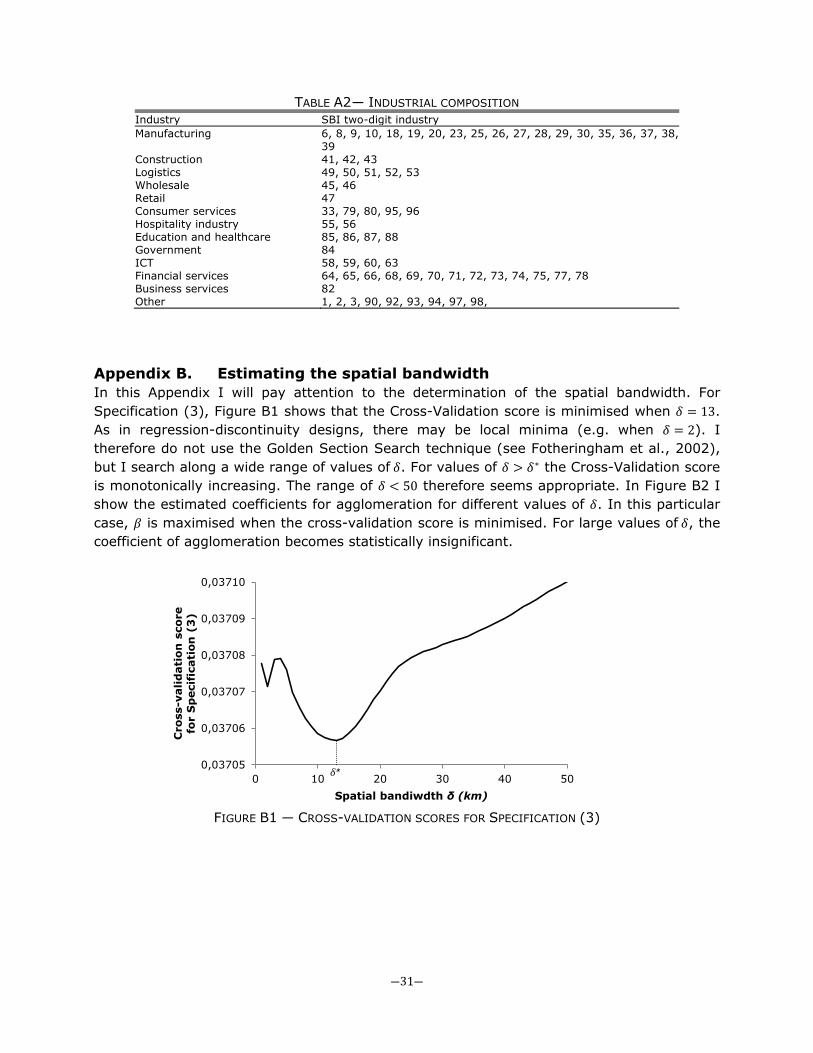
―31―

TABLE A2― INDUSTRIAL COMPOSITION Industry SBI two-digit industry Manufacturing 6, 8, 9, 10, 18, 19, 20, 23, 25, 26, 27, 28, 29, 30, 35, 36, 37, 38,

39 Construction 41, 42, 43 Logistics 49, 50, 51, 52, 53 Wholesale 45, 46 Retail 47 Consumer services 33, 79, 80, 95, 96 Hospitality industry 55, 56 Education and healthcare 85, 86, 87, 88 Government 84 ICT 58, 59, 60, 63 Financial services 64, 65, 66, 68, 69, 70, 71, 72, 73, 74, 75, 77, 78 Business services 82 Other 1, 2, 3, 90, 92, 93, 94, 97, 98,

Appendix B. Estimating the spatial bandwidth In this Appendix I will pay attention to the determination of the spatial bandwidth. For Specification (3), Figure B1 shows that the Cross-Validation score is minimised when 𝛿 = 13. As in regression-discontinuity designs, there may be local minima (e.g. when 𝛿 = 2). I therefore do not use the Golden Section Search technique (see Fotheringham et al., 2002), but I search along a wide range of values of 𝛿. For values of 𝛿 > 𝛿∗ the Cross-Validation score is monotonically increasing. The range of 𝛿 < 50 therefore seems appropriate. In Figure B2 I show the estimated coefficients for agglomeration for different values of 𝛿. In this particular case, 𝛽 is maximised when the cross-validation score is minimised. For large values of 𝛿, the coefficient of agglomeration becomes statistically insignificant.

FIGURE B1 ― CROSS-VALIDATION SCORES FOR SPECIFICATION (3)

δ* 0,03705

0,03706

0,03707

0,03708

0,03709

0,03710

0 10 20 30 40 50

Cro

ss-v

alid

atio

n s

core

fo

r S

pec

ific

atio

n (

3)

Spatial bandiwdth δ (km)

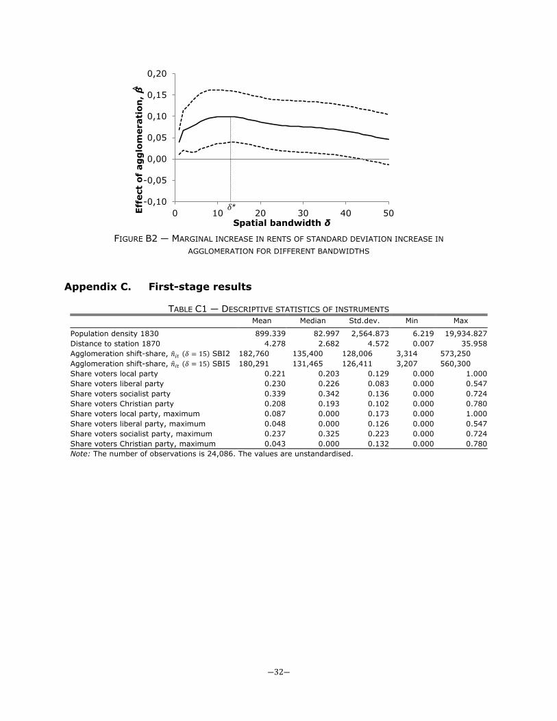
―32―

FIGURE B2 ― MARGINAL INCREASE IN RENTS OF STANDARD DEVIATION INCREASE IN

AGGLOMERATION FOR DIFFERENT BANDWIDTHS

Appendix C. First-stage results

TABLE C1 ― DESCRIPTIVE STATISTICS OF INSTRUMENTS Mean Median Std.dev. Min Max

Population density 1830 899.339 82.997 2,564.873 6.219 19,934.827 Distance to station 1870 4.278 2.682 4.572 0.007 35.958 Agglomeration shift-share, 𝑛�𝑗𝑡 (𝛿 = 15) SBI2 182,760.389 135,400.000 128,006.000 3,314.000 573,250.000 Agglomeration shift-share, 𝑛�𝑗𝑡 (𝛿 = 15) SBI5 180,291.000 131,465.000 126,411.000 3,207.000 560,300.000 Share voters local party 0.221 0.203 0.129 0.000 1.000 Share voters liberal party 0.230 0.226 0.083 0.000 0.547 Share voters socialist party 0.339 0.342 0.136 0.000 0.724 Share voters Christian party 0.208 0.193 0.102 0.000 0.780 Share voters local party, maximum 0.087 0.000 0.173 0.000 1.000 Share voters liberal party, maximum 0.048 0.000 0.126 0.000 0.547 Share voters socialist party, maximum 0.237 0.325 0.223 0.000 0.724 Share voters Christian party, maximum 0.043 0.000 0.132 0.000 0.780 Note: The number of observations is 24,086. The values are unstandardised.

δ*

<

-0,10

-0,05

0,00

0,05

0,10

0,15

0,20

0 10 20 30 40 50Effe

ct o

f ag

glo

mer

atio

n, β

Spatial bandwidth δ

―33―

TABLE C2 ― FIRST STAGE REGRESSION RESULTS (Dependent variable: the logarithm of rent per square meter)

(2) (4) (9) (12) (13)

IV – FE Population

density

IV– FE SBI two-

digit instrument

IV – FE SBI five-

digit instrument

IV – FE Political

instruments

IV – FE Political

instruments

Population density 1830 (log) -0.077 (0.008) *** Distance to station 1870 -0.032 (0.003) *** Agglomeration shift-share, 𝑛�𝑗𝑡 0.761 0.766 (0.013) *** (0.014) *** Share voters liberal party -0.026 -0.022 (0.004) *** (0.004) *** Share voters socialist party 0.090 0.053 (0.008) *** (0.006) *** Share voters Christian party -0.003 -0.012 (0.005) (0.005) ** Share voters liberal party, maximum

-0.004 0.009 (0.003) (0.003) ***

Share voters socialist party, maximum

-0.025 -0.009 (0.003) *** (0.004) **

Share voters Christian party, maximum

-0.004 0.010 (0.003) (0.003) ***

Control variables included (51) Yes Yes Yes Yes Yes PC6 fixed effects (8,461) Yes Yes Yes Yes Yes NUTS2-year fixed effects (180) No No No No Yes Function of location and year Θ( ∙ ) No No No No Yes Spatial bandwidth 𝛿∗ (in km) 18 17 17 10 13 R² First-stage 0.4074 0.9991 0.9991 0.9969 0.9983 F-Test weak instruments 103.218 3,187.732 2,816.425 194.023 135.929 Notes: See Table 1. All instruments are transformed to have zero mean and unit standard deviation.

Appendix D. Kernel functions Throughout the paper, I employ a Tricube kernel to estimate employment densities. The average weight for a Tricube function is relatively high, in contrast to the Exponential distance decay function, which decays much more quickly. For example, given a uniform distribution of employment and 𝛿 = 13, 95 percent for the weight of a Tricube weighting function is within 9 kilometres of the location, given a uniform distribution of employment over space. For a Triangular, Epanechnikov and Exponential distance decay function, this is respectively 10.09, 10.56 and 5.8 kilometres. Figure D1 illustrates the shapes of the different kernel functions. Figure D2 presents the cross-validation scores for three specifications with different kernel functions and highlights that the bandwidth is very similar for different kernel functions.

―34―

FIGURE D1 ― KERNEL FUNCTIONS

FIGURE D2 ― CROSS-VALIDATION SCORES FOR SPECIFICATIONS (3), (16), (17) AND (18)

δ δ 0.0

1.0

0.5

Wei

gh

t

TricubeTriangularEpanechnikovExponential

0,037050

0,037060

0,037070

0,037080

0,037090

0 5 10 15 20 25 30

Cro

ss-v

alid

atio

n s

core

Spatial bandwidth δ (km)

TricubeTriangularEpanechnikovExponential