rocky mountain power 1407 w. north temple street, room 220
TRANSCRIPT

Integra Realty Resources 5107 South 900 East T 801.263.9700 Salt Lake City Suite 200Suite 200 F 801.263.9709 Salt Lake City, Utah 84117 [email protected] www.irr.com/saltlakecity
January 16, 2019 Mr. Benjamin Clegg Rocky Mountain Power 1407 W. North Temple Street, Room 220 Salt Lake City, Utah 84116 SUBJECT: Opinion Letter – Impact of Electrical Transmission Line Upgrade on Home Values Dear Mr. Clegg,
It is my understanding that you are involved in a project to upgrade a ~60‐year old 46kV transmission line with a 138kV line. Based on this, you have asked that I summarize the implications to this matter of my research on home values and transmission lines. Please note that I have not looked specifically at this project nor any particular property(s). Instead, my opinion is informed by published studies my co‐authors and I conducted on the impact of transmission lines on home values in Salt Lake County. In our studies, copies of which are attached, we analyzed over 350,000 homes and 100,000 sales in Salt Lake County occurring from 2001 through 2014. We evaluated over 300 different home/property variables for the homes in order to isolate the impact on value of proximity to transmission lines. These studies represent the largest studies ever undertaken on this valuation issue.
Based on the results of our studies, upgrading an existing transmission corridor from 46kV to 138kV would have no impact to very nominal impact on immediately proximate homes. Though we did not specifically address pole design in our studies, it is my opinion based on our general research that any such impact would be eliminated or reduced further if general pole type is not meaningfully changed as a result of the voltage upgrade of the corridor.

2
If you have any questions or comments, please contact the undersigned. Thank you for the opportunity to be of service.
Respectfully submitted,
Integra Realty Resources ‐ Salt Lake City
Troy A. Lunt, MAI, SR/WA

Troy A. Lunt, MAI, SR/WA Salt Lake City Integra Realty Resources
irr.com
T 801.263.9700 F 801.263.9709
5107 South 900 East Suite 200 Salt Lake City, UT 84117
Experience Troy is a director and full time commercial real estate appraiser and consultant with Integra Realty Resources – Salt Lake City. He has been appraising since 1994 assisting commercial, governmental and private clients across a wide range of property and assignment types. Troy specializes in eminent domain/right‐of‐way valuation pertaining to surface, subsurface and aerial property interests. He also has considerable experience in forensic appraising and litigation consulting/expert services for a wide range of litigation actions including eminent domain, ad valorem taxation, corporate/ partnership dissolution and allocation, estate planning/resolution, divorce, and value impairment from all sources including environmental and regulatory. Troy has been qualified as an expert witness. Other areas of expertise include fundamental market analyses, feasibility studies, investment consultation and general commercial appraisal. Troy holds the MAI designation issued by the Appraisal Institute. Prior to joining Integra Realty Resources, he was a founding partner in the Fortis Group, a local appraising and consulting firm, and before that was a Director with LECG, an international expert services firm.
Professional Activities & Affiliations MAI, Appraisal Institute SR/WA, International Right of Way Association R/W‐AC, International Right of Way Association Affiliate Member Salt Lake Board of Realtors Past President/Current Board Member, Utah Chapter International Right of Way Association Utah Appraiser Board Experience Screening Committee, 2004 – present Board of Directors Utah Association of Appraisers, 2009 – present
Licenses Utah, Certified General, 5457226‐CG00 Nevada, Certified General, A.0206229‐CG Wyoming, Certified General, Permit 1060 Idaho, Certified General, CGA‐3399
Education
Bachelor of Arts, University of Utah, June 1994 Appraisal Principles Basic Income Capitalization Appraisal Procedures Highest and Best Uses Advanced Income Capitalization Report Writing & Valuation Analysis Advanced Applications Advanced Sales Comparison & Cost Approaches Uniform Standards of Professional Appraisal Practice Uniform Appraisal Standards for Federal Land Acquisitions Environmental Contamination Around Hill AFB Understanding Real Estate Investment Eminent Domain New Tools & Strategies Appraisal Laws & Legislation Current State of Wetlands Regulations Planning & Growth Issues Along the Wasatch Front Water Rights Valuation Challenges Environmental Issues in Real Estate Real Estate Finance Detrimental Conditions in Real Estate Valuation The Impact on Real Estate Changes in Tax Law
[email protected] ‐ 801.263.9700 x120

Troy A. Lunt, MAI, SR/WA Salt Lake City Integra Realty Resources
irr.com
T 801.263.9700 F 801.263.9709
5107 South 900 East Suite 200 Salt Lake City, UT 84117
Education (Cont'd) Evaluating Commercial Construction Eminent Domain & Condemnation Business Practices & Ethics New Technology for Real Estate Appraisers Scope of Work Feasibility, Market Value, Investment Timing: Option Value Condemnation Appraising: Principles & Applications Utah Eminent Domain Update (Presenter) Litigation Appraising: Specialized Topics & Applications International Right of Way SR/WA Comprehensive Exam Challenge Review Course National USPAP Equivalent Update Course Environmental Due Diligence & Liability Project Development & the Environmental Process The Valuation of Partial Acquisitions Eminent Domain Law: Basics for the Right of Way Professional Easement Valuation
Expert Testimony 2011 UDOT v. AF 1‐15 – Deposition 2011 UDOT v. Brown – Trial 2011 UDOT v. Dunsmure Long Term Investments, LLC, Et Al. – Deposition 2012 Cook v. SITLA – Deposition 2012 UDOT v. McDougal – Trial 2012 Salt Lake City v. Evans Development Group – Deposition 2012 Rocky Mountain Power v. Millerberg Holdings, LC – Deposition 2012 Giovengo Properties v. Hallmark Homes & Development – Deposition 2012 DL Evans Bank v. Clark Real Estate, Et Al. – Deposition 2013 Traverse Mountain v. Fox Ridge, LLC – Trial 2013 Windygates, LLC v. BMA Construction – Arbitration 2013 Salt Lake City v. Evans Development Group – Trial 2013 Davis County v. Aland Foundation – Trial 2014 UDOT v. Fort Lane Village, LLC – Deposition 2014 UTA v. D&S North Temple – Trial 2014 First Utah Bank v. Cottonwood Professional Plaza ‐ Trial 2014 UTA v. Fear Factory – Trial 2014 UDOT v. Sanchez – Trial 2014 Plumb v. Salt Lake County, Et Al. – Deposition & Trial 2015 Williamson v. Farrell – Deposition 2015 Rocky Mountain Power v. Marriott – Deposition 2015 Porter v. Morrell – Trial 2015 Bochner v. Durham Jones & Pinegar – Arbitration 2015 UDOT v. Target, Et Al. – Trial 2015 UDOT v. LEJ – Deposition & Trial 2015 UDOT v. Frontage 11400 ‐ Trial 2016 Bear River Insurance Company v. Ford Motor Company – Deposition 2017 Stromness MPO, LLC v. United States – Deposition & Trial 2017 Chard, Et Al. v. Chard, Et Al. ‐ Deposition 2018 Daufuskie Investments II v. Haws, Et Al. – Trial 2018 Taylor v. Paul Menlove Inc. – Deposition 2019 Marcantel v. Michael & Sonja Saltman Family Trust – Deposition
[email protected] ‐ 801.263.9700 x120
Articles and Publications “A Closer Look at Proximity Damages.” Right of Way. March/April 2016: Pages 32 – 36. “Property Value Impacts from Transmission Lines, Subtransmission Lines, and Substations,” The Appraisal Journal, Summer 2016, Pages 205 – 229
www.appraisalinstitute.org Summer2016•TheAppraisalJournal 205
Peer-ReviewedArticle
Introduction
Numerous previous quantitative studies have addressed the impact of power lines on property values. These studies have been carefully reviewed and summarized by a number of authors, including Colwell, 1990; Kroll and Priestley, 1992; Delaney and Timmons, 1992; Chalmers and Vooraart, 2009; Jackson and Pitts, 2010; and Haggerty, 2012.1 Such studies have yielded a mix of conclusions, ranging from no impact on prop-erty value to a negative impact of usually less than 10%. In virtually every study, any impact on
property value diminishes rapidly as the distance from the property to the power line increases. Unfortunately, these studies have a number of deficiencies, which may be attributable to the limited data sets on which these studies are based. In contrast, the current study includes a compre-hensive data set compiled for the largest counties in Utah, although the discussion in this article focuses specifically on Salt Lake County, the most populous county in the state. Using more comprehensive data, it is possible to address several important issues that have not been adequately analyzed in previous research
Property Value Impacts from Transmission Lines, Subtransmission Lines, and SubstationsbyTedTatos,MarkGlick,PhD,JD,andTroyA.Lunt,MAI
AbstractPriorresearchonthevalueimpactofproximitytotransmissionlineshasreliedonrelativelylimitedsamplesizes,
propertycharacteristics,andtypesoflines.Thisstudyextendsthepreviousresearchbyanalyzingalmostallsingle-
familyhomesalesoverafourteen-yearperiodforSaltLakeCounty,Utah,usingover125,000transactionsand
approximately450homecharacteristicstoexaminetheeffectsofvarioustypesoftransmissionlinesandofsubsta-
tions.Thislargesampleanalysispermitsestimationofthecountywideaggregateeffectsofthesefactorsonproperty
values.Theresultsfindsomenegativeeffectsthatdifferbytypeoftransmissionline,andasinpreviousresearch,
theeffectsdiminishwithdistance.Aswithsomepreviousresearch,theresultsalsoshowsomeevidenceofmodest
positiveeffectsassociatedwithproximitytolargetransmissionlines,whichmayberelatedtogreenwaysconstructed
beneathsuchlines.Ongoingresearchtoimprovethereliabilityofthestudyresultswillincludeconsiderationof
propertyrightsassociatedwiththetransmissioncorridorsandimpactonhomevaluesoffrontingroadtypes.
1. PeterF.Colwell,“PowerLinesandLandValue,”Journal of Real Estate Research5,no.1(1990):117–127;CynthiaKrollandThomas
Priestley,The Effects of Overhead Transmission Lines on Property Values: A Review and Analysis of the Literature(Washington,DC:Edison
ElectricInstituteSitingandEnvironmentalPlanningTaskForce,1992);CharlesJ.DelaneyandDouglasTimmons,“HighVoltagePowerLines:
DoTheyAffectResidentialPropertyValue?”Journal of Real Estate Research7,no.3(June1992):315–329;JamesA.ChalmersandFrank
A.Voorvaart,“High-VoltageTransmissionLines:Proximity,Visibility,andEncumbranceEffects,”The Appraisal Journal(Summer2009):
227–245;ThomasO.Jackson,andJenniferPitts,“TheEffectsofElectricTransmissionLinesonPropertyValues:ALiteratureReview,”
Journal of Real Estate Literature18,no.2(2010):239–259;andJuliaHaggerty,“TransmissionLinesandPropertyValueImpacts:ASummary
ofPublishedResearchonPropertyValueImpactsfromHighVoltageTransmissionLines”(reportpreparedbyHeadwatersEconomicsforthe
MountainStatesTransmissionIntertieReviewProject,May2012).

Peer-Reviewed Article
206TheAppraisalJournal•Summer2016 www.appraisalinstitute.org
studies. First, while previous research has focused on a specific neighborhood or even a single sub-division, the current study’s data set covers almost all single-family home sales in Salt Lake County from 2001 through 2014.2 Second, the transmission line data contains location information for all types of high-voltage and medium-voltage transmission lines (500 kV, 345 kV, 230 kV, 138 kV, 100 kV, and 46 kV) as well as substation locations.3 Consequently, it is possible to examine the effects of one type of line, e.g., 345 kV, while controlling for the effects of other types of lines. Previous research has either considered a single type of line4 or com-bined the effects of various types of power lines.5 Such simplifications, which are likely the by-product of limited data, can lead to erroneous estimates. For example, consider the impact of proximity to a 345 kV transmission line within 200 meters and beyond 200 meters. The presence of other types of transmission lines close to the properties studied, but omitted from the data, may significantly impact the indicated effects of the 345 kV lines. Third, the data includes almost all single- family home sales for all of Salt Lake County over a fourteen-year period, representing well over 100,000 sales. The depth and breadth of the data in the database allows investigation of the impacts of a wider range of property characteris-tics than has been considered in previous studies. The scope of the data also permits future investi-gation into the property-value impacts of other externalities, such as pipelines, road expansions, open-space areas, and research centers. Fourth, while previous studies often proxy the influence of macroeconomic factors by simply introducing time variables, this study directly tests the impact on price of macroeconomic fac-tors in order to isolate the influence of power lines on property values. Correctly accounting for such factors is essential in this case as the data begins before the housing crash in 2007, includes the entire recession, and stretches well
into the recovery period. Time dummy variables are included to capture any effects not included in the macroeconomic variables; this is discussed in more detail later. Finally, the data and methodology introduced here can be used to analyze the effects of many other changes to neighborhood infrastructure on property values, including mass transit, sources of solid waste and pollution, pipelines, roads, and, of particular interest to the Salt Lake region, prox-imity to earthquake and liquefaction risk areas.
Background on Transmission Lines and Substations
The current study is unique in that it simultane-ously, but separately, analyzes the impact of dif-ferent types of transmission lines on property values. It is important, therefore, to understand the different types of transmission lines that potentially impact property values. The starting point for electricity generation lies at the power plant. Generators at power plants generate elec-tricity at voltages that usually fall below 22 kV. Power must then be transmitted, often across long distances, to the areas where it will be con-sumed. To reduce energy loss, power is transmit-ted at very high voltages. In the United States, transmission lines voltages range up to 765 kV, with lines above 220 kV commonly referred to as extra-high-voltage transmission lines. The high-est-voltage line in Utah is 500 kV, though such lines are not located in Salt Lake County and are not considered in this analysis. The highest-volt-age lines in Salt Lake County are 345 kV, which are discussed in this analysis. Power plants use generating transformers to “step up” the voltage to transmission level. Very-high-voltage lines, such as 500 kV and 345 kV, then carry bulk power from the generating sta-tion to transmission substations near population centers. Power must then be transmitted across the entire area, which often includes hundreds
2. WhilethedatabasecoversothercountiesinUtah,thisstudyfocusesonSaltLakeCountybecause(1)wearewellfamiliarwiththearea,
(2)itisthemostpopulatedcountyinUtah,and(3)thereisarichtransmissionlinedataset.
3. DatawereobtainedfromtheUtahGeographicalSurvey.Substationlocationswereidentifiedaseithercompany-owned(PacifiCorp/Rocky
MountainPower)orprivatelyowned.
4. ChalmersandVoorvaart,“High-VoltageTransmissionLines.”
5. StanleyW.HamiltonandGregoryM.Swann,“DoHighVoltageTransmissionLinesAffectPropertyValue?”Land Economics71,no.4
(November1995):436–444.

Property Value Impacts from Transmission Lines, Subtransmission Lines, and Substations
www.appraisalinstitute.org Summer2016•TheAppraisalJournal 207
of thousands of homes. Large towers, such as the ones that support 500 kV and 345 kV lines, are not ubiquitous in population centers. Homes require voltages at much lower levels: 120 volts in the United States. Therefore, interconnected transformers at transmission substations “step down” the power to subtransmission voltages of generally between 46 kV and 138 kV. These subtransmission lines, which are commonly located along highways or arterial roads, then carry bulk power from major substations to regional and local distribution substations. Transmission line poles, such as those that carry 138 kV lines, can have under-built power dist-ribution lines as well as cable TV and commu-nications lines. Exhibit 1 illustrates such a configuration in Salt Lake County, Utah. The distribution substations, which are located close to consumers, then step down the voltage again to between 2 kV and 35 kV, which is con-
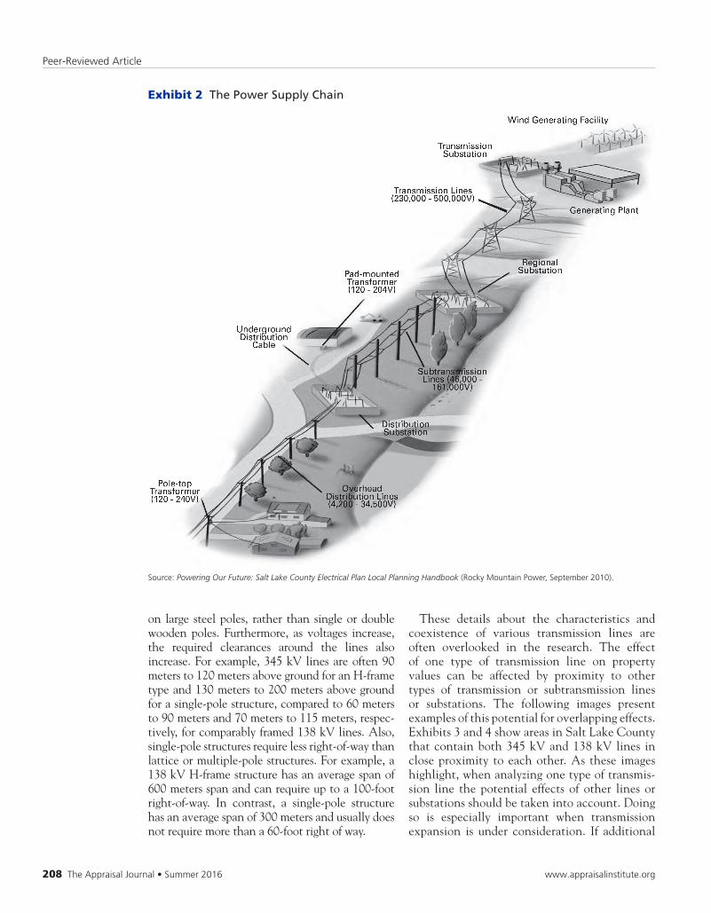
sidered medium voltage. Primary distribution lines then carry the power to distribution trans-formers near a customer location. The distribu-tion transformers, usually located on a wooden power pole, step down the voltage again to utili-zation voltage. Secondary distribution lines typi-cally service multiple customers, who connect using service drops, i.e., the line running from the home to the power pole. Exhibit 2 depict the electric power supply chain. This combination of power plants, substations, transmission lines, and distribution lines is known as the power grid. The study analysis only considers transmission lines, subtransmission lines, and substations in the power grid. Also, although the database contains other types of transmission lines, only the line types that exist in Salt Lake County are discussed. The types of transmission lines are distinguished not just by voltage, but also by the appearance. Higher-voltage transmission lines are often located
Source:MickeyBeaver,“SitingTransmissionLinesandSubstations,”SaltLakeCountyElectricalPlanTaskForce(RockyMountainPower,
December3,2009).
Exhibit 1 Double Circuit 138 kV Transmission Line with 12.5 kV Distribution Under-Build
Peer-Reviewed Article
208TheAppraisalJournal•Summer2016 www.appraisalinstitute.org
on large steel poles, rather than single or double wooden poles. Furthermore, as voltages increase, the required clearances around the lines also increase. For example, 345 kV lines are often 90 meters to 120 meters above ground for an H-frame type and 130 meters to 200 meters above ground for a single-pole structure, compared to 60 meters to 90 meters and 70 meters to 115 meters, respec-tively, for comparably framed 138 kV lines. Also, single-pole structures require less right-of-way than lattice or multiple-pole structures. For example, a 138 kV H-frame structure has an average span of 600 meters span and can require up to a 100-foot right-of-way. In contrast, a single-pole structure has an average span of 300 meters and usually does not require more than a 60-foot right of way.
These details about the characteristics and coexistence of various transmission lines are often overlooked in the research. The effect of one type of transmission line on property values can be affected by proximity to other types of transmission or subtransmission lines or substations. The following images present examples of this potential for overlapping effects. Exhibits 3 and 4 show areas in Salt Lake County that contain both 345 kV and 138 kV lines in close proximity to each other. As these images highlight, when analyzing one type of transmis-sion line the potential effects of other lines or substations should be taken into account. Doing so is especially important when transmission expansion is under consideration. If additional
Exhibit 2 The Power Supply Chain
Source:Powering Our Future: Salt Lake County Electrical Plan Local Planning Handbook(RockyMountainPower,September2010).

Property Value Impacts from Transmission Lines, Subtransmission Lines, and Substations
www.appraisalinstitute.org Summer2016•TheAppraisalJournal 209
lines are proposed in proximity to existing lines, ignoring the presence of those existing lines could result in overstating the impact on prop-erty values of the proposed lines. Neglecting the presence of each type of transmission line can affect the calculated impact on property values of one or the other type of line.
Study Database
The study database has been compiled from a number of sources. Transmission-line location data for the entire state of Utah was obtained from the Utah Geographical Survey in the form of a shapefile identifying transmission line locations at regular intervals for all individual transmission lines in Utah.6 The data, which contained approximately 165,000 coordinate points, also identified the types of transmission lines and the location of individual substations in Utah (Exhibit 5). For Salt Lake County, arm’s-length transaction sales and home characteristic data were obtained from the multiple listing service (MLS) and the county assessor’s computer-assisted mass appraisal (CAMA) databases. These data provided a fea-ture-rich array of variables identifying home and neighborhood characteristics. In addition to the variables provided, information was parsed from the “Remarks,” “Amenities,” “Interior Features,” and “Exterior Features” fields in the MLS data; many home characteristics that could impact value are included as comments in these fields. For example, various amenities, such as skylights, Trex decking, solar paneling, tankless water heat-ers, gourmet kitchens, types of cabinetry, have no fields associated with them so realtors and home-owners often list such information in the Remarks field. The parsing effort proved useful since the analysis could control for a greater number of home characteristics than in previous research. Geocoding data was also included in the form of latitude and longitude location of each home. These data were necessary in order to compute distances from each home to each point on each transmission line. The distance was calculated between each data point and the location of each of the approximately 350,000 properties in
Salt Lake County, for a total of over 60 billion computations. Next, the minimum distance from each property to each transmission line was calculated. Thus, the database includes data on
Exhibit 3 Transmission Lines near King’s Point Park, West Valley City, Utah
Source:©2015,GoogleEarth.
Exhibit 4 Transmission Lines and Substation, Bluffdale, Utah
Source:©2015,GoogleEarth.
6. ThesedatawerecodedinNorthAmericanDatum83,thedatumusedtoidentifythegeodeticnetworkinNorthAmerica.Wetranslated
thesepointsintolatitudeandlongitudecoordinates.

Peer-Reviewed Article
210TheAppraisalJournal•Summer2016 www.appraisalinstitute.org
the distance to every 345 kV, 230 kV, 138 kV, and 46 kV line and substation for every parcel. (In Salt Lake County there were no 500 kV, 230 kV, 100 kV, or 69 kV lines.) Each parcel in the assessor database was matched to each single-family home property sale during the period, as reported by the MLS. This matching resulted in a database that contains all sales infor-mation, including detailed characteristics as well as distances from each property to each type of transmission line and substation. Monthly eco-nomic variables (unemployment rate, housing starts, etc.) for Salt Lake County were based on data obtained from the Census Bureau.
Statistical Methodology
A hedonic regression model was used to estimate the property value impacts of proximity to vari-ous types of transmission lines. Hedonic analysis
enjoys ubiquitous use and acceptance as a statis-tical method, and it is recognized as a reliable technique of analyzing real estate transaction data. Hedonic analysis involves the valuation of a commodity as a function of its constituent parts, estimating the implicit price impact of each of those characteristics.7 Researchers often include additional variables to explain property values, such as economic factors, whether directly or by including time as a proxy. As is common for hedonic regression models, the sale price is estimated as a function of home charac-teristics and location variables. In addition, quarterly time dummies are included, using first quarter 2001 as the benchmark. Of course, time itself has little, if any, theoretical basis. Rather, it is used as a proxy for changing economic con-ditions or changing consumer preferences. For example, home sales in Utah generally dip during the winter season because of the difficult winters. Homes in certain neighborhoods, e.g.,
Exhibit 5 Location Overview: Utah and Salt Lake County High-Voltage Transmission Lines and Substations
7. Hedonicanalysisisoftenperformedusingregressionanalysis,leadingtothetermhedonic regression.Thistermsimplyreferstothe
useofregressionanalysistoestimateamodelwherethevalueofagoodisafunctionofitsindividualcharacteristics.Forexample,the
generalhedonicequationexpressestheproperty’spriceasafunctionofitsfeatures:Price=Constant+b1 Bedrooms+b2 Bathrooms+
b3 Lot Size…etc.
Utah Salt Lake County

Property Value Impacts from Transmission Lines, Subtransmission Lines, and Substations
www.appraisalinstitute.org Summer2016•TheAppraisalJournal 211
Olympus Cove, are often covered in snow, mak-ing marketing considerably more difficult. Although time dummies are a rough measure that offer limited insight into the actual impacts of changing market factors on property values, they are helpful in creating quality-adjusted price indices. Price indices are often of great interest to realtors, investors, home buyers and sellers, and researchers since these can be used to measure overall price changes controlling for the qualitative differences in property transac-tions. For example, the current analysis shows a significant difference between the quality-ad-justed and unadjusted indices in Salt Lake County beginning with the Great Recession. While the two indices generally followed each other before the recession, the quality-adjusted index shows a significantly greater drop than the
unadjusted index during the post-recession period (Exhibit 6). Such a result is not surprising. During the recession and the recovery the real estate market favored buyers, and higher-quality homes could be obtained at considerably lower prices. Thus, more high-quality homes were sold and more lesser-quality homes remained unsold. Such an effect would mask the actual drop in home prices, since, if the same quality of homes had been sold both pre- and post-recession, the drop would have been much greater. In the study, the sale price is also adjusted by netting out seller-paid concessions. Also, many of the sales have inclusions that could affect the price of the home, such as appliances, hot tubs, playgrounds, sheds, etc. To control for these inclusions, they are added as dummy
Exhibit 6 Differences between Quality-Adjusted and Unadjusted Home Price Indices, 2001–2014 by Quarter
Source:SaltLakeCountyMLSdata.
1.800
1.600
1.400
1.200
1.000
0.800
0.600
0.400
0.200
0.000
Pric
e In
dex
(1s
t q
uar
ter
2001
= 1
)
5,000
4,500
4,000
3,500
3,000
2,500
2,000
1,500
1,000
500
0
Nu
mb
er o
f Sa
les
YQ2001
_1
YQ2001
_3
YQ2002
_1
YQ2002
_3
YQ2003
_1
YQ2003
_3
YQ2004
_1
YQ2004
_3
YQ2005
_1
YQ2005
_3
YQ2006
_1
YQ2006
_3
YQ2007
_1
YQ2007
_3
YQ2008
_1
YQ2008
_3
YQ2009
_1
YQ2009
_3
YQ2010
_1
YQ2010
_3
YQ2011
_1
YQ2011
_3
YQ2012
_1
YQ2012
_3
YQ2013
_1
YQ2013
_3
YQ2014
_1
YQ2014
_3
AdjustedIndex UnadjustedIndex Sales

Peer-Reviewed Article
212TheAppraisalJournal•Summer2016 www.appraisalinstitute.org
variables in the regression model. Also, short sales and home auctions increased during the study period due to the recession, and it was necessary to control for short sales, auctions, and sales of bank-owned homes. In total, the model for Salt Lake County for the 2001–2014 period includes 127,584 observations and 450 explanatory variables. One of the key issues in hedonic analysis, and one that often receives less attention than warranted, is the handling of count variables, such as bedrooms, bathrooms, etc. These vari-ables often enter hedonic models in natural log form (e.g., ln_bedrooms, ln_bathrooms, ln_acreage). A different approach is used in this study, by creating individual binary (dummy) variables for the values taken by bedrooms, bath-rooms (whole bathrooms, half bathrooms, and three-quarter bathrooms are treated separately). This approach is preferred, because it avoids functional form assumptions with respect to these variables. Also, the dummy variable approach mitigates, at least in part, the obvious multicollinearity problem that arises from including both bedrooms and bathrooms in con-tinuous form. For quasi- continuous variables, such as acreage and square footage, the natural log form is used. For the key variables of interest—proximities to various types of transmission lines—dummy variables are created indicating whether homes are located within a certain radial distance from each type of transmission line. Then, the homes are grouped into distance categories, such as distances 50 meters or less, 50+–100 meters, 100+–150 meters, etc. For example, a property located 33 meters away from a 354 kV line and 77 meters away from a 138 kV line would be flagged with a 1 for the 100 meters or less category for the 345 kV line distance and a 1 for the 50+–100m category for the 138 kV line distance. It would receive a 0 in all other cat egories. Exhibit 7 shows the definitions of the distance variables. The final regression specification expresses the natural logarithm of sale price as a function of home characteristics, date identifiers, location factors, economic conditions, and transmission line proximities. As previously explained, prox-imities are expressed as dummy variables that indicate location in set distance bands around the transmission lines or substations. The regres-sion equation is as follows:
where:
HC = home characteristics, appearing in dummy vari-
ableform
LOC=locationdummies,identifyingspecificzipcodes
TL=distancedummies,indicatingproximityradii(e.g.,
propertyiswithin100meters)ofacertaintransmission
line type or a substation
EC = economic factors, including unemployment rate
andhousingstarts
YQ = dummy variables, indicating year and quarter.
These were included to capture any additional effects
thatwerenotcapturedbythemonthlyeconomicfactors.
Also addressed are two points that have been the subject of interest in this field: easements and the presence of power poles on the location. Easement information was obtained from Salt Lake County. This was included as a dummy variable in the model and, as expected, yielded a negative effect from the presence of an ease-ment. The easement variable results are not used to draw any conclusions, however, because there is a low frequency of easements, and to date, it has not been confirmed that the easements only include transmission line access. As part of con-tinued research, property-by-property investiga-tion is being undertaken to identify, among other things, properties where such power-line easements occur. Also part of the continuing research is an effort to identify the parcels on which power poles are located (although it is likely that poles located on residential parcels are dis tribution line poles, not transmission line poles). It is expected that there will be value impacts from poles located on residential parcels, and that such effects may extend to adjoining properties when the poles are located near lot lines. Determining these impacts will require a significant amount of research; such research would be aided signifi-cantly if utilities, which hold precise location data, became involved in the study. The next step in the analysis is to address var-ious data and statistical issues that often con-front researchers using hedonic analysis. These issues can be separated into four categories: spatial relationships, functional form, hetero-
n z y
ln(Price)=a +k bi(HC)+k bj(LOC )+k bk(TL)+i=1 j=1 k=1
v t
k bi(EC)+k bi(YQ)h=1 i=1

Property Value Impacts from Transmission Lines, Subtransmission Lines, and Substations
www.appraisalinstitute.org Summer2016•TheAppraisalJournal 213
skedasticity, and collinearity. Functional form, heteroskedasticity, and collinearity have received considerable attention in previous lit-erature. Spatial relationships, however, have begun to receive greater scrutiny only recently as geographic information systems (GIS) have gained popularity. Issues such as functional form distinctions and heteroskedasticity can be solved by addressing spatial relationships, commonly called spatial autocorrelation. Rather than adopt-ing computational solutions, the current study attempts to address spatial effects and other potential issues by including a large number of explanatory variables that capture the potential effects. Such variables may not be available for every study, as their collection is a time- consuming and perhaps impossible task given data limitations in specific studies. The large data set in the current study, however, does make it possible to address issues such as heteroskedas-ticity and spatial autocorrelation directly through analytical methods.8
Results Summary
The results over the entire 2001–2014 sample period indicate both practically and statistically significant effects from 138 kV and 69 kV lines but no negative effects from 345 kV lines. In fact, a slight positive effect was noted for prop-erties within 50 meters of 345 kV lines. This is discussed in more detail below. In addition, a negative effect is noted for close proximity (within 50 meters) to substations. A summary of the results regarding transmission lines and sub-stations appears in Exhibit 8; the full results are shown in the appendix at the end of this article. As Exhibit 8 shows, 138 kV lines appear to generate the most significant effects, both practi-cally and statistically. Homes within 50 meters of these lines see a 5.1% decrease in value, while the effect diminishes with distance. At 50+–100 meters, homes see a 2.9% decrease, while after 400 meters the effect drops below 1%. Somewhat of interest, homes within 50 meters of 46 kV lines see no effect, but homes 50+–100 meters see a 2.5% decrease. Beyond 200 meters, the effect for 46 kV lines drops to zero. Blockage of view may be one reason for this finding; the lines may actually be more noticeable by homes at a medium distance rather than directly adjacent. Since mountain views are an important positive factor in determining home values in Salt Lake County, this negative effect is not surprising. Finally, the results show that proximate location to substations (≤ 50 meters) is associated with a 2.9% decrease in value. The results with regard to 345 kV lines are interesting, since one would expect that these larger transmission lines would have a commen-surate negative effect on property values, but this is not the case for the entire sample. The location of these lines was closely investigated by conducting site visits and examining aerial photography, and this showed that homes abut-ting 345 kV corridors often benefit from open space unavailable to other homes. For example, the corridor might include a greenway and path amenity, as shown Exhibit 9. Further, since no other homes can be built on the corridor, homes adjacent to the corridor may benefit from view-shed and less crowding.
Variable Type of Line Proximity
TL_345_100 345kV ≤ 100 meters
TL_345_100_200 345kV 100+–200meters
TL_345_200_300 345kV 200+–300meters
TL_345_300_400 345kV 300+–400meters
TL_138_50 138kV ≤50meters
TL_138_50_100 138kV 50+–100meters
TL_138_100_200 138kV 100+–200meters
TL_138_200_300 138kV 200+–300meters
TL_138_300_400 138kV 300+–400meters
TL_46_50 46kV ≤50meters
TL_46_50_100 46kV 50+–100meters
TL_46_100_200 46kV 100+–200meters
TL_46_200_300 46kV 200+–300meters
TL_46_300_400 46kV 300+–400meters
TL_SUBCO_50 Substation ≤50meters
TL_SUBCO_50_100 Substation 50+–100meters
Exhibit 7 Definitions of Distance Variables
8. In-depthinformationonissuesrelatedtostatisticalsignificanceandfunctionalformcanbeobtainedbycontactingtheauthors.

Peer-Reviewed Article
214TheAppraisalJournal•Summer2016 www.appraisalinstitute.org
Time Model ResultsThe study results cover the entire period from 2001 through 2014. In addition to quantifying any distance effects, the data is analyzed to deter-mine whether the effects change over time. Salt Lake County experienced considerable develop-ment during the study period, particularly in the southern and western portions. As such, an inter-esting question is whether consumer preferences changed over the study period given additional development, economic changes due to the Great Recession, and, as a potential result, the diver-gence between adjusted and unadjusted price indices in Salt Lake County. Given the behavior
of the indices, it was postulated that during buy-ers’ markets the effects of transmission lines may be amplified. The attractiveness of neighbor-hoods in high demand may mute some of the effects of the transmission lines, particularly if those precise neighborhood characteristics can-not be fully controlled in the hedonic model. To investigate the interaction of market changes over time and transmission line effects, the sample population was divided into the fol-lowing temporal subsets of sales: 2001–2004, 2005–2008, 2009–2011, 2012–2014. Then, the model was run separately on these subsets to observe any changes in the effects of transmission
Variable Type of Line Proximity Effect Size* Pr > | t |† VIF‡
Intercept 8.95476 <.0001 0
TL_345_100 345kV ≤ 100 meters 0.94% 0.286 1.05525
TL_345_100_200 345kV 100+–200meters 0.85% 0.217 1.0778
TL_345_200_300 345kV 200+–300meters 0.88% 0.104 1.09186
TL_345_300_400 345kV 300+–400meters 0.65% 0.174 1.0888
TL_138_50 138kV ≤50meters -5.10% <.0001 1.02982
TL_138_50_100 138kV 50+–100meters -2.91% <.0001 1.04463
TL_138_100_200 138kV 100+–200meters -2.09% <.0001 1.12057
TL_138_200_300 138kV 200+–300meters -1.85% <.0001 1.11169
TL_138_300_400 138kV 300+–400meters -1.11% <.0001 1.10736
TL_46_50 46kV ≤50meters -0.49% 0.399 1.14255
TL_46_50_100 46kV 50+–100meters -2.53% <.0001 1.10109
TL_46_100_200 46kV 100+–200meters -0.94% <.0001 1.16574
TL_46_200_300 46kV 200+–300meters 0.19% 0.303 1.10713
TL_46_300_400 46kV 300+–400meters 0.27% 0.103 1.08094
TL_SUBCO_50 Substation ≤50meters -2.92% 0.052 2.39144
TL_SUBCO_50_100 Substation 50+–100meters -0.38% 0.845 2.24569
Exhibit 8 Summary of Results
* Effect sizeisthecoefficientindicatingtheeffectofeachvariable(i.e.,theparameterestimate).
† Pr > |t|isthep-valueindicatingtheprobabilityofobservinganeffectaslargeorlargeriftheassumptionofnoeffectweretrue(i.e.,ifthenull
hypothesisweretrue).Inotherwords,ifweassumethatthisvariablehasnoeffectonprice,whatistheprobabilitythattherewouldbean
effectsizeaslargeorlargerthanwhatisobservedintheregression.Typically,ap-valuelessthan0.05isconsideredstatisticallysignificant,
thoughthestudyfocusismoreonthepracticaleffectsizeratherthanthestatisticalsignificance,especiallygiventhesamplesize.
‡ VIFisthevarianceinflationfactor.TheVIFsindicatehowthepresenceofmulticollinearityinflatesthevarianceofanestimatorbyexamining
howoneexplanatory variable canbeexplainedby the remainingexplanatory variables in themodel. Ifnocollinearityexists, theVIFofa
coefficientwill be1.GenerallyVIF valuesabove5or10are considered indicatorsofamulticollinearityproblem.SeeA.H.Studenmund,
Using Econometrics—A Practical Guide4thed.,at258 (“While there isno tableof formalcriticalVIFvalues,acommonruleof thumb is
thatifVIF(bi)>5,themulticollinearityissevere.”).SeealsoDamodarGujarati,Basic Econometrics3rded.,at339(“Asaruleofthumb,ifthe
VIFofavariableexceeds10(thiswillhappeniftheR2exceeds0.90),thatvariableissaidtobehighlycollinear.”).

Property Value Impacts from Transmission Lines, Subtransmission Lines, and Substations
www.appraisalinstitute.org Summer2016•TheAppraisalJournal 215
lines. Exhibit 10 shows the number of observa-tions, the resulting fit of each time subset model, and the effect sizes with corresponding p-values. The time model results offer several findings of note. First, with respect to 138 kV lines, the effect on homes within 50 meters is the strongest in the most recent sample subset (2012–2014), with a negative effect of approximately -7%. Moreover, the findings show the opposite of what was originally expected. The effects were higher during the prerecession seller’s market (2005–2008), coming in at -6.8%, and lower during the recession and immediately post-re-cession period (2009–2011), coming in at -5.3%. Second, the time model indicates most-pro-nounced negative effects from 345 kV lines occurred in the more recent samples (2012–2014), coming in at -4.6%, although these effects diminish at distances beyond 100 meters. The time model results also offer some caution-ary notes. The most recent period shows by far the lowest number of sales. The 2012–2014 period has fewer than half the number of sales per year compared with the first two periods, and only 63% of the sales of the immediately preced-ing 2008–2011 period, which included the reces-sion. These findings indicate that examining small samples of more recent data may yield sub-stantially different estimates than large samples that cover a longer period. Further, while some studies have found that effects on value from proximity to transmission lines may dissipate over time, this study does not confirm such an effect. The findings presented here indicate that other potential factors could explain temporal effects, such as the state of the economy as a whole, regional employment, and supply and demand effects. If such factors are correlated with the passage of time, researchers may erroneously attribute diminishing proximity effects to the passage of time alone, while, in reality, other factors drive the effect. Consequently, care should be taken when including time variables. While time variables, either as dummy variables or time trends, can add significant explanatory power to a regression (usually in the form of increased R2), these time factors serve as proxies for the underlying economic mechanism(s) driv-ing the effect. The researcher must always keep in mind the purpose of the study when estimating the regression. A high R2, with a high percentage of the variation in the depen-
dent variable (e.g., prices) being explained by the model may be a visually pleasing statistic, but such comfort is misleading if the true purpose of the regression is to predict or inves-tigate the effects of a particular variable or set of variables, such as proximity to transmission lines. Therefore, future research should con-tinue to examine temporal effects on proximity to transmission lines.
Conclusion
It should be noted that the foregoing results do not account for property rights considerations for abutting transmission corridors. While 345 kV corridors often exist in fee, 138 kV and 46 kV corridors typically involve only easements. Fur-ther, the data have not yet been qualified as to location of the lines relative to the properties (front yard, rear yard, etc). These refinements should allow more precise isolation of specific elements that may impact values of homes prox-imate to transmission lines. Application of similar studies in other market areas is essential to improve the extrapolative reliability of any proximity study results. Over the past several years, we have assembled sales data nationwide and anticipate identifying other mar-
Exhibit 9 Transmission Line Greenway
Source:Powering Our Future: Salt Lake County Electrical Plan Local Planning Handbook
(RockyMountainPower,September2010).

Peer-Reviewed Article
216TheAppraisalJournal•Summer2016 www.appraisalinstitute.org
Variable Model 2001–2004 Model 2005–2008 Model 2009–2011 Model 2012–2014
EFFECT_ESMT -0.0597(0.0001) 0.5536(0.0000) -0.4084(0.0110) -0.1820(0.0017)
STREET_1W 0.0153(0.5916) -0.0578(0.0164) 0.0237(0.4644) 0.1281(0.0107)
STREET_2W -0.0535(0.0000) -0.0552(0.0000) -0.0230(0.0070) 0.0276(0.0046)
STREET_4L -0.1238(0.0000) -0.1727(0.0004) -0.0570(0.1282) -0.0596(0.0952)
STREET_CS -0.0468(0.0000) -0.0518(0.0000) -0.0141(0.1163) 0.0359(0.0006)
STREET_DE -0.0529(0.0000) -0.0648(0.0000) -0.0304(0.0066) 0.0343(0.0098)
STREET_EX -0.2581(0.0000) -0.2834(0.0000) -0.2335(0.0000) -0.1752(0.0000)
STREET_HW -0.0906(0.0003) -0.1161(0.0000) -0.1087(0.0000) -0.0550(0.0241)
STREET_RW -0.1019(0.0000) -0.0897(0.0008) -0.0775(0.0138) -0.0105(0.8123)
TL_138_100_200 -0.0179(0.0004) -0.0265(0.0000) -0.0158(0.0554) -0.0155(0.0806)
TL_138_200_300 -0.0243(0.0000) -0.0194(0.0000) -0.0199(0.0058) -0.0050(0.4958)
TL_138_300_400 -0.0165(0.0000) -0.0107(0.0037) -0.0104(0.0765) -0.0102(0.1528)
TL_138_50 -0.0210 (0.2233) -0.0684 (0.0000) -0.0532 (0.0160) -0.0698 (0.0146)
TL_138_50_100 -0.0273(0.0046) -0.0494(0.0000) -0.0060(0.6697) -0.0220(0.2087)
TL_345_100 0.0251 (0.0431) 0.0306 (0.0031) 0.0014 (0.9486) -0.0461 (0.1125)
TL_345_100_200 0.0201(0.0432) 0.0004(0.9564) 0.0274(0.1409) 0.0060(0.7751)
TL_345_200_300 0.0247(0.0004) 0.0019(0.7975) 0.0151(0.2223) -0.0130(0.3365)
TL_345_300_400 0.0109(0.1145) 0.0075(0.2232) 0.0085(0.4018) -0.0220(0.0425)
TL_46_100_200 -0.0030(0.4409) -0.0113(0.0008) -0.0220(0.0002) -0.0154(0.0227)
TL_46_200_300 0.0038(0.2299) 0.0024(0.4089) -0.0029(0.5461) -0.0033(0.5625)
TL_46_300_400 0.0027(0.3449) 0.0044(0.0886) -0.0049(0.2595) 0.0044(0.3937)
TL_46_50 -0.0151(0.0815) 0.0067(0.4855) -0.0303(0.0628) 0.0043(0.7778)
TL_46_50_100 -0.0207 (0.0011) -0.0244 (0.0000) -0.0358 (0.0006) -0.0282 (0.0179)
TL_SUBCO_100_200 -0.0049(0.7501) 0.0108(0.4477) 0.0107(0.6806) -0.0030(0.9186)
TL_SUBCO_200_300 -0.0121(0.1558) -0.0015(0.8341) -0.0062(0.6102) 0.0123(0.3458)
TL_SUBCO_50 -0.0472(0.0852) -0.0110(0.6063) -0.0227(0.5394) 0.0274(0.5181)
TL_SUBCO_50_100 0.0035 (0.9126) 0.0108 (0.7119) -0.0196 (0.7114) -0.0362 (0.4842)
Exhibit 10 Time Model Results
p-valuesindicatedinparentheses
Model Observations Used Adj. R-Squared
2001–2004 42,001 89.8%
2005–2008 47,084 92.8%
2009–2011 23,638 90.6%
2012–2014 14,863 92.0%

Property Value Impacts from Transmission Lines, Subtransmission Lines, and Substations
www.appraisalinstitute.org Summer2016•TheAppraisalJournal 217
ket areas for study in the short term. Furthermore, while the foregoing study specifically addresses electrical transmission corridors, the data and methodology introduced here can be used to ana-lyze other types of rights-of-way, including road-ways, petroleum and natural gas pipelines, water and wastewater pipelines, and mass-transit routes. In addition, the same data and models can be used in analyzing other geospatial value questions, such as correlation between home value and prox-imity to negative externalities (e.g., correctional facilities, sources of pollution, solid waste facili-
ties) or positive externalities (e.g., public parks, universities, transit stations), and even value impacts of higher-risk areas associated with natu-ral disasters, such as flooding, earthquakes/lique-faction, landslides, wildfires, and high winds. Finally, the data and methodologies allow for the reliable analysis of value impacts associated with issues with considerable political implica-tions, such as correlation between improving performance of neighborhood schools and home values or the impact on home value of adding energy-efficiency elements, such as solar panels.
About the AuthorsTed TatosisadirectoratEmpiricalAnalytics,aneconomicsandstatisticalconsultingfirmspecializinginquantitative
analysisandlitigationsupport.HealsohasbeenanadjunctprofessorofeconomicsandstatisticsattheUniversityof
Utah.TatosreceivedhisBAineconomicsfromDukeUniversityandMSinstatisticsfromtheUniversityofUtah.Hehas
analyzedpropertyvalueissuesthroughhedonicmodelingandanalyticsforvariousprivatesectorclientsoverthelast
twentyyears.TatosisalsoaprincipaliniQuantix,adataanalyticsfirmthatcombineseconomic,statistical,and
valuationexpertise.Contact: [email protected]
Mark Glick, PhD, JD,isaprofessorofeconomicsandanadjunctprofessoroflawandtheUniversityofUtah.He
receivedhisBAandMAatUCLA,hisPhDattheNewSchoolforSocialResearch,andhisJDfromColumbiaUniversity.
Hehaspublishedoverthirtyprofessionalarticlesandbooksonissuesrelatedtolawandeconomics.Heiscurrentlyof
counselwiththelawfirmofParsons,Behle&Latimer.Contact: [email protected]
Troy A. Lunt, MAI, SR/WA,isamanagingdirectorwiththeSaltLakeCityofficeofIntegraRealtyResources.His
primarypracticeareasareright-of-wayandlitigationsupport.Lunthasbeenappraisingrealestateforovertwenty
yearsandhereceivedhisMAIdesignationin2004.HehasaBSinorganizationalcommunicationsfromtheUniversity
ofUtah.HeisaprincipaliniQuantix,adataanalyticsfirmthatcombineseconomic,statistical,andvaluationexpertise.
Contact: [email protected]
AcknowledgmentsThisresearchstudywasnotsupportedbyanyfundingfromanyindustry,academic,orotherpublicorprivatesources.
Theauthorsself-fundedallresearch,datagathering,andanalysis.TheauthorswouldliketothankDavidBuell,with
theUtahAutomatedGeographicReferenceCenter;DavidBaird,withCaldwellRealty;SaltLakeCountyAssessorKevin
Jacobs;andJaromZenger,withtheSaltLakeCountyAssessor’sOfficefortheirvaluableassistancewiththisresearch.
CONTINUED>

Peer-Reviewed Article
218TheAppraisalJournal•Summer2016 www.appraisalinstitute.org
TL_345_100 0.009 0.009 1.070 0.286
TL_345_100_200 0.009 0.007 1.230 0.217
TL_345_200_300 0.009 0.005 1.620 0.104
TL_345_300_400 0.007 0.005 1.360 0.174
TL_138_50 -0.051 0.010 -5.240 <.0001
TL_138_50_100 -0.029 0.006 -4.770 <.0001
TL_138_100_200 -0.021 0.003 -6.410 <.0001
TL_138_200_300 -0.018 0.003 -6.530 <.0001
TL_138_300_400 -0.011 0.003 -4.300 <.0001
TL_46_50 -0.005 0.006 -0.840 0.399
TL_46_50_100 -0.025 0.004 -6.510 <.0001
TL_46_100_200 -0.009 0.002 -4.250 <.0001
TL_46_200_300 0.002 0.002 1.030 0.303
TL_46_300_400 0.003 0.002 1.630 0.103
TL_SUBCO_50 -0.029 0.015 -1.940 0.052
TL_SUBCO_50_100 -0.004 0.020 -0.200 0.845
TL_SUBCO_100_200 0.002 0.009 0.200 0.842
TL_SUBCO_200_300 -0.003 0.005 -0.730 0.464
HILLSIDE 0.019 0.002 9.380 <.0001
RAISEDROOF 0.017 0.003 6.140 <.0001
EFFECT_ESMT -0.072 0.067 -1.080 0.281
EFFECT_FLOD -0.025 0.103 -0.240 0.812
STREET_HW -0.102 0.007 -13.990 <.0001
STREET_2W -0.046 0.003 -14.930 <.0001
STREET_1W 0.003 0.010 0.330 0.739
STREET_CS -0.038 0.003 -11.480 <.0001
STREET_DE -0.047 0.004 -11.570 <.0001
STREET_RW -0.097 0.011 -8.640 <.0001
STREET_4L -0.129 0.010 -13.240 <.0001
STREET_EX -0.267 0.011 -23.820 <.0001
TOPO_MTN 0.024 0.012 1.970 0.049
TOPO_ROL 0.031 0.002 16.700 <.0001
ZIP_84006 -0.048 0.147 -0.330 0.743
ZIP_84020 0.112 0.013 8.700 <.0001
ZIP_84044 -0.077 0.033 -2.310 0.021
ZIP_84047 0.118 0.026 4.610 <.0001
ZIP_84065 0.066 0.040 1.660 0.097
ZIP_84070 0.118 0.017 6.950 <.0001
ZIP_84081 0.031 0.016 1.890 0.059
ZIP_84084 0.044 0.016 2.730 0.006
ZIP_84088 0.046 0.016 2.860 0.004
Appendix Full Results
Variable Parameter Estimate Standard Error t -Value Pr > | t |
Intercept 8.955 0.035 256.630 <.0001

Property Value Impacts from Transmission Lines, Subtransmission Lines, and Substations
www.appraisalinstitute.org Summer2016•TheAppraisalJournal 219
ZIP_84090 0.257 0.075 3.420 0.001
ZIP_84091 0.315 0.147 2.140 0.033
ZIP_84092 0.187 0.017 11.030 <.0001
ZIP_84093 0.191 0.017 11.430 <.0001
ZIP_84094 0.121 0.017 7.150 <.0001
ZIP_84095 0.079 0.038 2.080 0.037
ZIP_84096 0.064 0.040 1.620 0.105
ZIP_84102 0.371 0.012 30.760 <.0001
ZIP_84103 0.572 0.013 42.530 <.0001
ZIP_84104 -0.050 0.011 -4.420 <.0001
ZIP_84105 0.429 0.012 37.140 <.0001
ZIP_84106 0.269 0.012 23.300 <.0001
ZIP_84107 0.105 0.012 8.690 <.0001
ZIP_84108 0.484 0.012 41.300 <.0001
ZIP_84109 0.329 0.012 28.120 <.0001
ZIP_84110 0.169 0.074 2.280 0.022
ZIP_84111 0.145 0.012 11.840 <.0001
ZIP_84112 -0.065 0.104 -0.630 0.530
ZIP_84113 0.078 0.085 0.920 0.357
ZIP_84114 0.000 . . .
ZIP_84115 0.119 0.012 10.320 <.0001
ZIP_84116 0.023 0.013 1.740 0.081
ZIP_84117 0.254 0.012 21.100 <.0001
ZIP_84118 -0.003 0.011 -0.280 0.776
ZIP_84119 -0.007 0.011 -0.590 0.552
ZIP_84120 -0.013 0.011 -1.140 0.253
ZIP_84121 0.186 0.012 15.930 <.0001
ZIP_84123 0.089 0.012 7.560 <.0001
ZIP_84124 0.275 0.012 23.290 <.0001
ZIP_84126 -0.060 0.085 -0.710 0.478
ZIP_84127 0.006 0.104 0.060 0.956
ZIP_84128 -0.026 0.012 -2.240 0.025
ZIP_84129 0.003 0.014 0.200 0.840
ZIP_84150 0.140 0.104 1.350 0.177
ZIP_84152 0.505 0.147 3.440 0.001
ZIP_84157 0.072 0.147 0.490 0.624
ZIP_84170 -0.065 0.085 -0.760 0.446
ZIP_84171 0.305 0.104 2.940 0.003
NSCoord -0.000 0.000 -1.970 0.049
EWCoord -0.000 0.000 0.000 0.998
EAST 0.106 0.003 38.100 <.0001
SOUTH 0.015 0.007 2.210 0.027
Appendix (continued )
Variable Parameter Estimate Standard Error t -Value Pr > | t |

Peer-Reviewed Article
220TheAppraisalJournal•Summer2016 www.appraisalinstitute.org
NUM_STORIES 0.022 0.002 12.100 <.0001
BATHFULL1 0.028 0.005 5.750 <.0001
BATHFULL2 0.063 0.005 12.370 <.0001
BATHFULL3 0.107 0.005 19.580 <.0001
BATHFULL4 0.169 0.007 24.820 <.0001
BATHFULL5 0.269 0.011 25.380 <.0001
BATHFULL6 0.341 0.020 17.190 <.0001
BATHHAL1 0.023 0.001 19.590 <.0001
BATHHAL2 0.086 0.004 20.580 <.0001
BATHHAL3 0.177 0.016 10.780 <.0001
BATHHAL4 0.255 0.060 4.260 <.0001
BATHHAL5 -0.016 0.104 -0.150 0.877
BATHTQ1 0.030 0.001 24.450 <.0001
BATHTQ2 0.053 0.002 22.490 <.0001
BATHTQ3 0.119 0.008 15.260 <.0001
BATHTQ4 0.344 0.025 13.540 <.0001
BATHTQ5 0.753 0.104 7.230 <.0001
BATHTQ6 0.820 0.104 7.920 <.0001
BED_1 -0.097 0.007 -13.470 <.0001
BED_2 -0.008 0.004 -1.850 0.064
BED_3 0.006 0.004 1.620 0.106
BED_4 0.007 0.004 1.960 0.050
BED_5 0.002 0.004 0.480 0.630
BED_6 0.009 0.004 2.380 0.017
TotFamRm -0.002 0.001 -2.470 0.014
TotFire 0.017 0.001 25.070 <.0001
TotFormal 0.008 0.005 1.560 0.119
TotKitch -0.002 0.001 -2.340 0.019
TotLdy 0.014 0.002 9.020 <.0001
TotSemi 0.002 0.001 2.110 0.035
LNHOUSINGST 0.021 0.003 6.960 <.0001
UNEMPLOYMENT_RATE 0.028 0.182 0.150 0.879
LISTTYPE_EAL -0.006 0.003 -2.040 0.041
AUCTION -0.158 0.012 -12.790 <.0001
ASISFIXER -0.070 0.002 -41.510 <.0001
FORECL_NBO 0.015 0.008 1.980 0.048
LNSQFT 0.387 0.003 150.680 <.0001
LNACRES 0.134 0.001 108.710 <.0001
LNAGE -0.094 0.001 -112.760 <.0001
NEWHOME 0.018 0.003 6.470 <.0001
SHORTSALE -0.055 0.002 -27.070 <.0001
HASBAR 0.011 0.001 11.190 <.0001
Appendix (continued )
Variable Parameter Estimate Standard Error t -Value Pr > | t |

Property Value Impacts from Transmission Lines, Subtransmission Lines, and Substations
www.appraisalinstitute.org Summer2016•TheAppraisalJournal 221
BsmntFin 0.000 0.000 25.030 <.0001
HASDECK 0.007 0.001 7.550 <.0001
GaragCap 0.002 0.000 15.240 <.0001
STYLE_RAMBLERRANCH -0.067 0.003 -20.980 <.0001
STYLE_2STORY -0.056 0.003 -17.230 <.0001
STYLE_BUNGALOW -0.061 0.003 -18.320 <.0001
STYLE_TRIMULTI -0.053 0.003 -15.390 <.0001
STYLE_SPLITENTR -0.063 0.004 -18.060 <.0001
STYLE_MANUFMOD -0.363 0.009 -41.410 <.0001
STYLE_CABIN 0.060 0.027 2.230 0.026
STYLE_TUDOR 0.079 0.006 13.620 <.0001
STYLE_MOBILE -0.562 0.015 -37.670 <.0001
STYLE_VICTORIAN 0.004 0.006 0.670 0.503
STYLE_AFRAME -0.141 0.030 -4.770 <.0001
STYLE_CAPECOD 0.019 0.010 1.840 0.066
ACCESS_ASPHALT 0.009 0.003 3.290 0.001
ACCESS_DIRT -0.047 0.008 -6.100 <.0001
ACCESS_GRAVEL 0.004 0.005 0.850 0.395
ACCESS_CIRCULAR 0.056 0.014 4.100 <.0001
ACCESS_CONCRETE 0.006 0.001 4.620 <.0001
ACCESS_COMMONDRIVE 0.009 0.006 1.550 0.121
OWNER_BANK -0.030 0.002 -12.880 <.0001
OWNER_HOMESTEPS -0.049 0.005 -10.430 <.0001
HEAT_FRCAIR_CENTGAS 0.001 0.001 0.910 0.362
HEAT_CENTGAS 0.005 0.002 2.840 0.005
HEAT_FRCAIR 0.007 0.002 4.260 <.0001
AMEN_SOLARPANELS 0.092 0.034 2.740 0.006
AMEN_HEATDRIVE 0.073 0.015 5.010 <.0001
AMEN_TREXDECK 0.009 0.004 2.150 0.032
AMEN_MUDROOM 0.025 0.008 3.220 0.001
AMEN_SKYLIGHT 0.016 0.005 3.320 0.001
AMEN_WICLOSET 0.003 0.003 1.220 0.221
AMEN_GARDENTUB -0.012 0.004 -3.120 0.002
AMEN_JETTEDTUB -0.015 0.002 -6.140 <.0001
AMEN_ELECTRICDRYER-
HOOKUP
-0.002 0.001 -2.470 0.013
AMEN_CABLETVWIRED 0.001 0.001 1.460 0.145
AMEN_CABLETVAVAILABLE 0.000 0.001 0.020 0.981
AMEN_GASDRYERHK 0.003 0.001 2.730 0.006
AMEN_HOMEWARR 0.001 0.001 0.590 0.552
AMEN_PARKPLAY -0.014 0.002 -7.130 <.0001
AMEN_POOL 0.024 0.004 6.260 <.0001
Appendix (continued )
Variable Parameter Estimate Standard Error t -Value Pr > | t |

Peer-Reviewed Article
222TheAppraisalJournal•Summer2016 www.appraisalinstitute.org
AMEN_WORKSHOP 0.002 0.002 1.060 0.290
AMEN_EXERCRM 0.027 0.003 9.290 <.0001
AMEN_CLUBHOUSE 0.014 0.004 3.700 0.000
AMEN_TENNISCOURT 0.016 0.005 3.460 0.001
AMEN_SAUNASTEAM 0.043 0.005 8.140 <.0001
AMEN_GATEDCOMM 0.032 0.009 3.480 0.001
AIR_CENT_ELEC 0.030 0.001 28.340 <.0001
AIR_CENT_GAS 0.031 0.002 13.990 <.0001
INCL_RANGE 0.001 0.001 1.060 0.291
INCL_MICROWAVE 0.017 0.001 16.420 <.0001
INCL_CEILINGFAN -0.004 0.001 -4.310 <.0001
INCL_WINDOWCOVRS 0.003 0.001 3.270 0.001
INCL_FRIDGE 0.017 0.001 17.430 <.0001
INCL_RANGEHOOD 0.006 0.001 5.980 <.0001
INCL_STORAGESHED -0.006 0.001 -4.950 <.0001
INCL_ALARMSYS 0.018 0.001 13.690 <.0001
INCL_SATDISHOREQ -0.002 0.001 -2.330 0.020
INCL_FIREPLACEINS -0.009 0.002 -6.140 <.0001
INCL_DWPORT 0.003 0.002 1.860 0.063
INCL_BASKETBALLST 0.003 0.002 2.020 0.044
INCL_SWINGSET -0.000 0.002 -0.060 0.949
INCL_HUMID 0.009 0.002 4.210 <.0001
INCL_TVANTENNA -0.004 0.002 -2.130 0.033
INCL_HOTTUB 0.009 0.002 4.420 <.0001
INCL_WOODSTOVE -0.020 0.002 -8.830 <.0001
INCL_DOGRUN -0.000 0.002 -0.150 0.883
INCL_COMPACTOR 0.017 0.003 6.300 <.0001
INCL_FREEZER -0.004 0.004 -1.050 0.295
INCL_WORKBENCH 0.014 0.004 3.190 0.001
INCL_GASGRILLBBQ 0.006 0.004 1.590 0.111
INCL_ELEAIRCLNR 0.012 0.004 3.060 0.002
INCL_GAZEBO 0.002 0.004 0.580 0.563
INCL_TRAMPOLINE 0.018 0.008 2.100 0.035
INCL_PLAYGYM 0.019 0.008 2.300 0.022
INCL_WATERSOFT 0.005 0.001 4.090 <.0001
INCL_PROJECTOR 0.052 0.016 3.270 0.001
INCL_DRYER_ONLY -0.003 0.003 -0.770 0.442
INCL_WASHER_ONLY 0.008 0.003 2.470 0.014
FINT_OAKCAB -0.008 0.003 -2.640 0.008
FINT_MAPLECAB -0.003 0.003 -0.980 0.325
FINT_ALDERCAB 0.020 0.003 7.690 <.0001
FINT_CHERRYCAB 0.053 0.006 8.380 <.0001
Appendix (continued )
Variable Parameter Estimate Standard Error t -Value Pr > | t |

Property Value Impacts from Transmission Lines, Subtransmission Lines, and Substations
www.appraisalinstitute.org Summer2016•TheAppraisalJournal 223
FINT_CSTMKITCHEN 0.046 0.004 11.180 <.0001
FINT_CANLIGHTS 0.007 0.006 1.150 0.249
FINT_MAHOGWDWK 0.044 0.026 1.690 0.090
FINT_CORIANCNTR 0.009 0.005 1.810 0.070
FINT_RADIANTHEAT 0.021 0.010 2.140 0.032
FINT_TANKLESS 0.042 0.016 2.720 0.007
FINT_WINECELLAR 0.095 0.019 5.100 <.0001
FINT_OPENFLOOR 0.002 0.002 1.110 0.267
FINT_TILEBATH 0.002 0.006 0.290 0.771
FINT_NEWCARPET 0.025 0.001 16.750 <.0001
FINT_DW 0.014 0.001 10.810 <.0001
FINT_DISP 0.000 0.001 0.150 0.878
FINT_MASTERBATH -0.014 0.001 -11.780 <.0001
FINT_WICLOSET 0.003 0.001 2.490 0.013
FINT_VCEILING -0.003 0.001 -2.980 0.003
FINT_UPDTKITCHEN 0.030 0.001 27.830 <.0001
FINT_GASLOG -0.001 0.001 -0.450 0.656
FINT_BATHSEPTUB 0.013 0.001 9.510 <.0001
FINT_DENOFFICE 0.019 0.001 15.990 <.0001
FINT_JETTUB 0.011 0.001 7.390 <.0001
FINT_GASRANGE 0.013 0.001 8.710 <.0001
FINT_FRDOORS 0.015 0.001 11.170 <.0001
FINT_RANGEBLT 0.001 0.001 0.530 0.597
FINT_GASOVEN 0.002 0.002 1.210 0.228
FINT_RANGECTOP -0.008 0.002 -3.850 0.000
FINT_DOUBLEOVEN 0.045 0.002 19.010 <.0001
FINT_CENTRALVAC 0.052 0.002 24.850 <.0001
FINT_SECKITCHEN 0.003 0.003 1.070 0.286
FINT_WETBAR 0.022 0.002 10.750 <.0001
FINT_GRANCNTR 0.045 0.002 25.160 <.0001
FINT_WALLOVEN 0.005 0.003 1.950 0.051
FINT_GREATROOM 0.022 0.003 6.500 <.0001
FINT_ALARM 0.018 0.004 5.110 <.0001
FINT_INTERCOM 0.015 0.003 4.660 <.0001
FINT_LAUNDCHUTE -0.004 0.003 -1.460 0.144
FINT_DRYBAR -0.002 0.003 -0.610 0.544
FINT_FLOORDRAIN 0.012 0.004 2.640 0.008
FINT_FIREALARM 0.015 0.004 3.460 0.001
FINT_RANGEDVENT 0.004 0.005 0.700 0.485
FINT_THEATERROOM 0.022 0.009 2.490 0.013
FINT_SILECOUNTER 0.050 0.011 4.710 <.0001
FINT_APT -0.027 0.003 -9.620 <.0001
Appendix (continued )
Variable Parameter Estimate Standard Error t -Value Pr > | t |

Peer-Reviewed Article
224TheAppraisalJournal•Summer2016 www.appraisalinstitute.org
BASEMNT_FULL -0.022 0.002 -14.580 <.0001
BASEMNT_PARTIAL 0.007 0.002 4.180 <.0001
BASEMNT_NONECRAWLSPACE 0.064 0.002 26.070 <.0001
BASEMNT_DAYLIGHT 0.001 0.001 0.750 0.456
BASEMNT_WALKOUT 0.004 0.002 2.470 0.013
BASEMNT_ENTRANCE -0.002 0.002 -1.350 0.177
LANDSCAPE_FULL 0.029 0.001 21.210 <.0001
LANDSCAPE_MATURETREES 0.005 0.001 4.600 <.0001
LANDSCAPE_FRUITTREES -0.010 0.001 -9.040 <.0001
LANDSCAPE_VEGGARDEN 0.001 0.001 1.150 0.249
LANDSCAPE_PART -0.018 0.002 -11.120 <.0001
LANDSCAPE_PINES 0.005 0.001 3.710 0.000
LANDSCAPE_TERRYARD 0.002 0.002 0.990 0.324
LANDSCAPE_SCRUBOAK 0.018 0.003 5.960 <.0001
LANDSCAPE_STREAM 0.082 0.005 18.010 <.0001
LANDSCAPE_WATERFALL 0.035 0.007 4.710 <.0001
LANDSCAPE_XERISCAPED 0.048 0.007 6.560 <.0001
FEXT_DOUBLEPANEWINDOWS 0.010 0.001 10.000 <.0001
FEXT_SLIDINGGLASSDOORS -0.012 0.001 -11.800 <.0001
FEXT_BAYBOXWINDOWS 0.006 0.001 5.220 <.0001
FEXT_OUTDOORLIGHTING 0.005 0.001 4.740 <.0001
FEXT_PORCHOPEN -0.005 0.001 -4.690 <.0001
LOT_CITYVIEW 0.023 0.007 3.280 0.001
LOT_SIDEWALKS -0.004 0.001 -3.810 0.000
LOT_SPRINKLERAUTO 0.019 0.001 17.170 <.0001
LOT_TERRAINFLAT 0.003 0.001 3.090 0.002
LOT_VIEWMOUNTAIN -0.003 0.001 -3.130 0.002
LOT_FENCEDFULL 0.004 0.001 2.690 0.007
LOT_ROADPAVED -0.002 0.001 -2.610 0.009
LOT_FENCEDPART 0.000 0.001 0.310 0.759
LOT_SECLYARD 0.008 0.001 7.280 <.0001
LOT_CULDESAC -0.010 0.002 -6.230 <.0001
LOT_PRIVATE 0.008 0.002 5.380 <.0001
LOT_CORNERLOT -0.010 0.001 -8.010 <.0001
LOT_VIEWVALLEY -0.006 0.002 -3.570 0.000
LOT_TERRGRADSLOPE 0.001 0.002 0.660 0.509
LOT_WOODED 0.027 0.002 10.920 <.0001
LOT_SPRINKRMAN 0.008 0.002 3.870 0.000
LOT_VIEWLAKE 0.027 0.004 7.120 <.0001
LOT_TERRMTN -0.014 0.005 -2.820 0.005
LOT_TERRHILL -0.010 0.005 -2.120 0.034
LOT_TERRSTEEPSLP -0.027 0.005 -4.950 <.0001
Appendix (continued )
Variable Parameter Estimate Standard Error t -Value Pr > | t |

Property Value Impacts from Transmission Lines, Subtransmission Lines, and Substations
www.appraisalinstitute.org Summer2016•TheAppraisalJournal 225
LOT_DRIPIRRIG 0.030 0.005 5.880 <.0001
LOT_ADDTLLANDAVL 0.017 0.008 2.150 0.031
LOT_ADJTOGOLFCRS 0.046 0.018 2.520 0.012
LOT_DRIPIRRMAN 0.005 0.018 0.300 0.764
EXTR_ALUMINUMVINYL -0.009 0.001 -8.680 <.0001
EXTR_BRICK 0.006 0.001 5.510 <.0001
EXTR_STUCCO 0.012 0.001 8.980 <.0001
EXTR_STONE 0.026 0.002 17.120 <.0001
EXTR_CEDARREDWOOD -0.007 0.002 -3.160 0.002
EXTR_FRAME -0.013 0.002 -6.280 <.0001
FLOOR_CHERRY 0.038 0.011 3.530 0.000
FLOOR_OAK 0.014 0.007 2.040 0.042
FLOOR_MAPLE 0.006 0.008 0.790 0.430
FLOOR_HICKORY 0.040 0.010 3.810 0.000
FLOOR_HANDSCRAPE 0.008 0.011 0.700 0.485
FLOOR_CARPET 0.009 0.002 5.180 <.0001
FLOOR_TILE 0.017 0.001 17.350 <.0001
FLOOR_HARDWOOD 0.023 0.001 23.000 <.0001
FLOOR_LINOLEUM -0.022 0.001 -20.210 <.0001
FLOOR_LAMINATE -0.003 0.003 -1.060 0.290
FLOOR_VINYL -0.028 0.004 -7.490 <.0001
FLOOR_MARBLE 0.079 0.003 25.110 <.0001
FLOOR_TRAVERT 0.059 0.004 14.040 <.0001
FLOOR_SLATE 0.029 0.005 6.180 <.0001
FLOOR_BAMBOO 0.045 0.007 6.760 <.0001
FLOOR_NATROCK 0.043 0.014 3.000 0.003
FLOOR_CORK 0.091 0.019 4.650 <.0001
FLOOR_HEATED 0.061 0.017 3.520 0.000
ROOF_ASPHALTSHIN -0.005 0.002 -1.890 0.059
ROOF_ASBESTOSSHIN -0.012 0.004 -3.210 0.001
ROOF_TARGRAVEL -0.029 0.003 -8.670 <.0001
ROOF_TILE 0.024 0.005 5.090 <.0001
ROOF_WOODSHAKESH 0.031 0.004 7.200 <.0001
ROOF_ALUMINUM -0.010 0.005 -2.010 0.044
ROOF_RUBBEREPDM 0.007 0.004 1.660 0.097
ROOF_FLAT -0.005 0.013 -0.410 0.682
ROOF_COMPOSITION -0.019 0.005 -4.080 <.0001
ROOF_PITCHED 0.007 0.004 1.880 0.060
ROOF_ROLLEDSILVER -0.030 0.007 -4.140 <.0001
POOL_INCLUDED 0.026 0.003 8.300 <.0001
WINDOW_WOOD 0.027 0.013 2.080 0.037
WINDOW_VINYL 0.004 0.003 1.270 0.204
Appendix (continued )
Variable Parameter Estimate Standard Error t -Value Pr > | t |
Peer-Reviewed Article
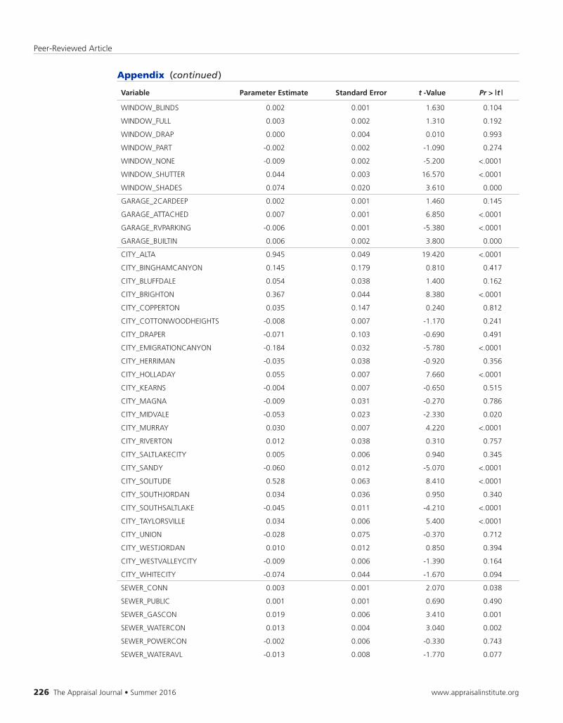
226TheAppraisalJournal•Summer2016 www.appraisalinstitute.org
WINDOW_BLINDS 0.002 0.001 1.630 0.104
WINDOW_FULL 0.003 0.002 1.310 0.192
WINDOW_DRAP 0.000 0.004 0.010 0.993
WINDOW_PART -0.002 0.002 -1.090 0.274
WINDOW_NONE -0.009 0.002 -5.200 <.0001
WINDOW_SHUTTER 0.044 0.003 16.570 <.0001
WINDOW_SHADES 0.074 0.020 3.610 0.000
GARAGE_2CARDEEP 0.002 0.001 1.460 0.145
GARAGE_ATTACHED 0.007 0.001 6.850 <.0001
GARAGE_RVPARKING -0.006 0.001 -5.380 <.0001
GARAGE_BUILTIN 0.006 0.002 3.800 0.000
CITY_ALTA 0.945 0.049 19.420 <.0001
CITY_BINGHAMCANYON 0.145 0.179 0.810 0.417
CITY_BLUFFDALE 0.054 0.038 1.400 0.162
CITY_BRIGHTON 0.367 0.044 8.380 <.0001
CITY_COPPERTON 0.035 0.147 0.240 0.812
CITY_COTTONWOODHEIGHTS -0.008 0.007 -1.170 0.241
CITY_DRAPER -0.071 0.103 -0.690 0.491
CITY_EMIGRATIONCANYON -0.184 0.032 -5.780 <.0001
CITY_HERRIMAN -0.035 0.038 -0.920 0.356
CITY_HOLLADAY 0.055 0.007 7.660 <.0001
CITY_KEARNS -0.004 0.007 -0.650 0.515
CITY_MAGNA -0.009 0.031 -0.270 0.786
CITY_MIDVALE -0.053 0.023 -2.330 0.020
CITY_MURRAY 0.030 0.007 4.220 <.0001
CITY_RIVERTON 0.012 0.038 0.310 0.757
CITY_SALTLAKECITY 0.005 0.006 0.940 0.345
CITY_SANDY -0.060 0.012 -5.070 <.0001
CITY_SOLITUDE 0.528 0.063 8.410 <.0001
CITY_SOUTHJORDAN 0.034 0.036 0.950 0.340
CITY_SOUTHSALTLAKE -0.045 0.011 -4.210 <.0001
CITY_TAYLORSVILLE 0.034 0.006 5.400 <.0001
CITY_UNION -0.028 0.075 -0.370 0.712
CITY_WESTJORDAN 0.010 0.012 0.850 0.394
CITY_WESTVALLEYCITY -0.009 0.006 -1.390 0.164
CITY_WHITECITY -0.074 0.044 -1.670 0.094
SEWER_CONN 0.003 0.001 2.070 0.038
SEWER_PUBLIC 0.001 0.001 0.690 0.490
SEWER_GASCON 0.019 0.006 3.410 0.001
SEWER_WATERCON 0.013 0.004 3.040 0.002
SEWER_POWERCON -0.002 0.006 -0.330 0.743
SEWER_WATERAVL -0.013 0.008 -1.770 0.077
Appendix (continued )
Variable Parameter Estimate Standard Error t -Value Pr > | t |
Property Value Impacts from Transmission Lines, Subtransmission Lines, and Substations
www.appraisalinstitute.org Summer2016•TheAppraisalJournal 227
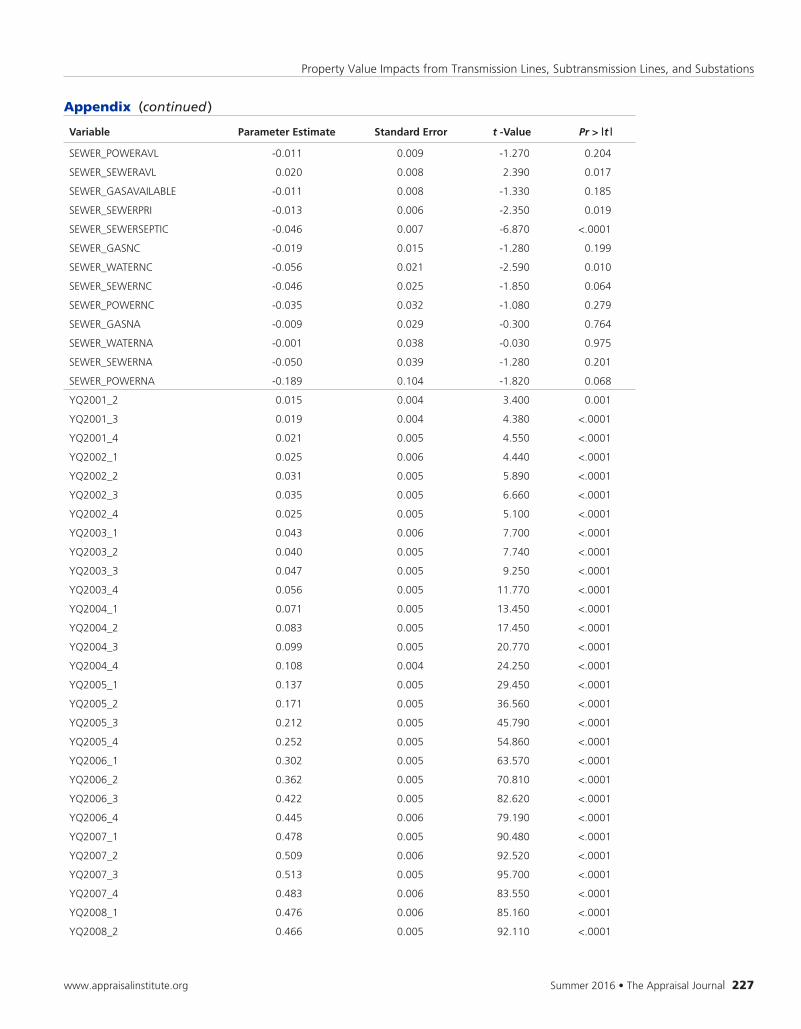
SEWER_POWERAVL -0.011 0.009 -1.270 0.204
SEWER_SEWERAVL 0.020 0.008 2.390 0.017
SEWER_GASAVAILABLE -0.011 0.008 -1.330 0.185
SEWER_SEWERPRI -0.013 0.006 -2.350 0.019
SEWER_SEWERSEPTIC -0.046 0.007 -6.870 <.0001
SEWER_GASNC -0.019 0.015 -1.280 0.199
SEWER_WATERNC -0.056 0.021 -2.590 0.010
SEWER_SEWERNC -0.046 0.025 -1.850 0.064
SEWER_POWERNC -0.035 0.032 -1.080 0.279
SEWER_GASNA -0.009 0.029 -0.300 0.764
SEWER_WATERNA -0.001 0.038 -0.030 0.975
SEWER_SEWERNA -0.050 0.039 -1.280 0.201
SEWER_POWERNA -0.189 0.104 -1.820 0.068
YQ2001_2 0.015 0.004 3.400 0.001
YQ2001_3 0.019 0.004 4.380 <.0001
YQ2001_4 0.021 0.005 4.550 <.0001
YQ2002_1 0.025 0.006 4.440 <.0001
YQ2002_2 0.031 0.005 5.890 <.0001
YQ2002_3 0.035 0.005 6.660 <.0001
YQ2002_4 0.025 0.005 5.100 <.0001
YQ2003_1 0.043 0.006 7.700 <.0001
YQ2003_2 0.040 0.005 7.740 <.0001
YQ2003_3 0.047 0.005 9.250 <.0001
YQ2003_4 0.056 0.005 11.770 <.0001
YQ2004_1 0.071 0.005 13.450 <.0001
YQ2004_2 0.083 0.005 17.450 <.0001
YQ2004_3 0.099 0.005 20.770 <.0001
YQ2004_4 0.108 0.004 24.250 <.0001
YQ2005_1 0.137 0.005 29.450 <.0001
YQ2005_2 0.171 0.005 36.560 <.0001
YQ2005_3 0.212 0.005 45.790 <.0001
YQ2005_4 0.252 0.005 54.860 <.0001
YQ2006_1 0.302 0.005 63.570 <.0001
YQ2006_2 0.362 0.005 70.810 <.0001
YQ2006_3 0.422 0.005 82.620 <.0001
YQ2006_4 0.445 0.006 79.190 <.0001
YQ2007_1 0.478 0.005 90.480 <.0001
YQ2007_2 0.509 0.006 92.520 <.0001
YQ2007_3 0.513 0.005 95.700 <.0001
YQ2007_4 0.483 0.006 83.550 <.0001
YQ2008_1 0.476 0.006 85.160 <.0001
YQ2008_2 0.466 0.005 92.110 <.0001
Appendix (continued )
Variable Parameter Estimate Standard Error t -Value Pr > | t |

Peer-Reviewed Article
228TheAppraisalJournal•Summer2016 www.appraisalinstitute.org
YQ2008_3 0.450 0.005 87.180 <.0001
YQ2008_4 0.414 0.006 71.890 <.0001
YQ2009_1 0.378 0.009 44.180 <.0001
YQ2009_2 0.346 0.008 44.380 <.0001
YQ2009_3 0.344 0.008 40.850 <.0001
YQ2009_4 0.332 0.008 39.410 <.0001
YQ2010_1 0.317 0.010 33.290 <.0001
YQ2010_2 0.292 0.008 34.840 <.0001
YQ2010_3 0.250 0.009 28.730 <.0001
YQ2010_4 0.218 0.008 26.730 <.0001
YQ2011_1 0.178 0.008 21.060 <.0001
YQ2011_2 0.172 0.007 24.110 <.0001
YQ2011_3 0.177 0.007 25.210 <.0001
YQ2011_4 0.146 0.007 21.330 <.0001
YQ2012_1 0.152 0.007 21.700 <.0001
YQ2012_2 0.200 0.006 33.360 <.0001
YQ2012_3 0.230 0.006 38.420 <.0001
YQ2012_4 0.253 0.006 42.420 <.0001
YQ2013_1 0.293 0.006 46.800 <.0001
YQ2013_2 0.351 0.005 65.570 <.0001
YQ2013_3 0.373 0.005 68.020 <.0001
YQ2013_4 0.356 0.006 59.330 <.0001
YQ2014_1 0.369 0.006 58.380 <.0001
YQ2014_2 0.397 0.006 70.200 <.0001
YQ2014_3 0.407 0.006 72.410 <.0001
YQ2014_4 0.399 0.007 59.430 <.0001
IRR_LOT 0.001 0.001 0.660 0.508
P1_LAUNDRY -0.008 0.001 -7.500 <.0001
P1_BEDROOM 0.009 0.002 3.860 0.000
P1_FULLBATH -0.009 0.002 -4.060 <.0001
P1_FORMALDINING 0.021 0.005 4.010 <.0001
Appendix (continued )
Variable Parameter Estimate Standard Error t -Value Pr > | t |

Property Value Impacts from Transmission Lines, Subtransmission Lines, and Substations
www.appraisalinstitute.org Summer2016•TheAppraisalJournal 229
Additional ReadingSuggestedbytheAuthors
Anselin,Luc.“TheMoranScatterplotasanESDATooltoAssessLocalInstabilityinSpatialAssociation.”InSpatial Analytical Perspectives on GIS,editedbyManfredM.Fischer,HenkJ.Scholten,andDavidUnwin,121–138.London:
TaylorandFrancis.Ltd.,1996.
Beaver,Mickey.“SitingTransmissionLinesandSubstations.”SaltLakeCountyElectricalPlanTaskForce.Rocky
MountainPower,December3,2009.
Berger,JamesO.“CouldFisher,Jeffreys,andNeymanHaveAgreedonTesting?”Statistical Science18,no.1(February
2003):1–12.
Bloomquist,Glenn.“TheEffectofElectricUtilityPowerPlantLocationonAreaPropertyValue.”Land Economics50,
no.1(February1974):97–100.
Cliff,A.D.,andJ.K.Ord.Spatial Processes: Models and Applications(London:PionLtd.,1981).
Cliff,JoelP.,andPaulWaddell.“AHedonicRegressionofHomePricesinKingCounty,Washington,UsingActivity-
SpecificAccessibilityMeasures.”Proceedings of the Transportation Research Board 82nd Annual Meeting.Washing-
ton,DC,2003.
Furby,Lita,RobinGregory,PaulSlovic,andBaruchFischoff.“ElectricPowerTransmissionLines,PropertyValues,and
Compensation.”Journal of Environmental Management27(January1988):69–83.
Geary,R.C.“TheContiguityRatioandStatisticalMapping.”The Incorporated Statistician5,no.3(November1954):
115–146.
Hubbard,Raymond,andM.J.Bayarri.“P-ValuesAreNotErrorProbabilities.”November2003.
Kinnard,WilliamN.,Jr.,andSueAnnDickey.“APrimeronImpactResearch:ResidentialPropertyValuesNear
High-VoltageTransmissionLines.”Real Estate Issues20,no.1(April1995):23–29.
Kroll,CynthiaA.“PropertyValuation:APrimeronProximityImpactResearch.”PaperpresentedatConferenceon
ElectricandMagneticFields,February1994.
Moran,P.A.P.“NotesonContinuousStochasticPhenomena,”Biometrika37,no.1-2(1950):17–23.
Mueller,JulieM.,andJohnB.Loomis.“SpatialDependenceinHedonicPropertyModels:DoDifferentCorrectionsfor
SpatialDependenceResultinEconomicallySignificantDifferencesinEstimatedImplicitPrices?”Journal of Agricul-tural and Resource Economics33,no.2(August2008):212–231.
Pitts,Jennifer,andThomasO.Jackson.“PowerLinesandPropertyValuesRevisited.”The Appraisal Journal(Fall2007):
323–325.
Wilson,AlbertR.“ProximityStigma:TestingtheHypothesis.”The Appraisal Journal(Summer2004):253–262.
Additional ResourcesSuggestedbytheY.T.andLouiseLeeLumLibrary
Appraisal Institute Lum Library External Information Sources [Login required] InformationFiles—RealEstateDamages,ProximityImpact
Electric Power Research Institute http://my.epri.com
Federal Energy Regulatory Commission—Transmission Line Siting http://www.ferc.gov/industries/electric/indus-act/siting.asp
US Department of Energy http://www.energy.gov
US Energy Information Administration http://www.eia.gov/
32 Right of Way M arch/April 2 0 1 6
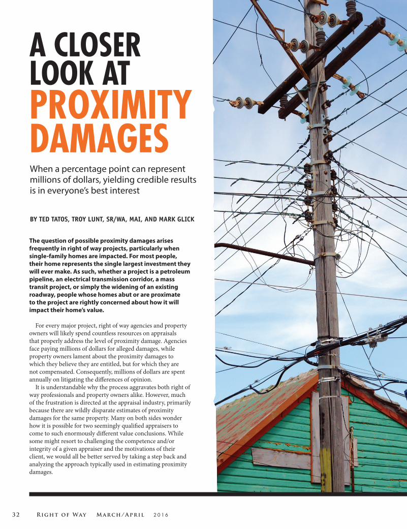
The question of possible proximity damages arises frequently in right of way projects, particularly when single-family homes are impacted. For most people, their home represents the single largest investment they will ever make. As such, whether a project is a petroleum pipeline, an electrical transmission corridor, a mass transit project, or simply the widening of an existing roadway, people whose homes abut or are proximate to the project are rightly concerned about how it will impact their home’s value.
For every major project, right of way agencies and property owners will likely spend countless resources on appraisals that properly address the level of proximity damage. Agencies face paying millions of dollars for alleged damages, while property owners lament about the proximity damages to which they believe they are entitled, but for which they are not compensated. Consequently, millions of dollars are spent annually on litigating the differences of opinion.
It is understandable why the process aggravates both right of way professionals and property owners alike. However, much of the frustration is directed at the appraisal industry, primarily because there are wildly disparate estimates of proximity damages for the same property. Many on both sides wonder how it is possible for two seemingly qualified appraisers to come to such enormously different value conclusions. While some might resort to challenging the competence and/or integrity of a given appraiser and the motivations of their client, we would all be better served by taking a step back and analyzing the approach typically used in estimating proximity damages.
BY TED TATOS, TROY LUNT, SR/WA, MAI, AND MARK GLICK
When a percentage point can represent millions of dollars, yielding credible results is in everyone’s best interest
A CLOSER LOOK AT PROXIMITY DAMAGES

March/April 2 0 1 6 Right of Way 33
Standing Up to ScrutinyIt is not unusual for one appraiser to use paired sales and published studies that indicate no damages, while another appraiser might use paired sales and published studies that suggest damages of 10 percent or more. This variance could potentially be avoided if the question of proximity damages were not addressed merely as part of another appraisal assignment, but were instead its own assignment.
The scope of such an assignment should be to analyze proximity impacts using data and methodologies that stand up to scrutiny not only by appraisers, but also by experts in associated fields such as statistics and economics, something that paired sales and most published studies on proximity impacts do not. While the costs of such a study would obviously be much greater than a typical appraisal, it would yield better project results when faced with balancing the need to treat property owners fairly with the need to prudently allocate agency or company funds.
Recognizing the unreliability and often wild inconsistencies of the status quo, some right of way agencies have commissioned larger studies. And while some of these studies have been published, most of them only address proximity impacts from electrical transmission corridors. These studies have generally reflected value impacts that are only loosely connected to corridor characteristics such as width, voltage, location on property and associated property rights. While the variance appears modest, an understatement or overstatement of
damages by only a few percentage points could easily translate into millions of dollars annually—either allocated to or withheld from property owners.
With significant financial impacts to right of way agencies and property owners alike, questions regarding the credibility of a given study in estimating proximity impacts become very practical for the right of way community. Exacerbating the saliency of these questions for the right of way community is the fact that certain federal agencies, such as the Federal Energy Regulatory Commission, have become increasingly concerned with the impact that right of way projects have on the value of abutting or proximate properties. Unfortunately, even cursory review of the scope and methodology of currently available studies indicates that proximity impacts are not being adequately analyzed, even when larger studies have been commissioned.
Addressing the InadequaciesThe most serious shortcomings of the published studies are lack of analytical rigor, limited scope of data and time, failure to use the latest advances in geocoding and computing, and failure to consider differences in the type or scope of corridors. Resolving these shortcomings requires that practitioners and their clients alike reconsider the assignment scope. To ensure that a proximity impact analysis will yield credible results requires significantly more data than is reflected in currently available studies. Additionally, the modeling must
Getting a Fair ShareWhen an appraiser is hired to value a partial acquisition, the primary assignment is determining the before and after valuation and any resulting damages. The proximity impact determination is usually relegated to a secondary consideration. As such, if the appraisal fee is only a few thousand dollars for the entire assignment, it’s likely that a relatively small portion will be allocated to the question of damages.
Consequently, the scope of work that is practical in analyzing proximity impacts is limited, even if appraisers are unwilling to admit it. As a result, the appraiser’s primary research on proximity impacts is likely to be some form of paired sales analysis that attempts to quantify proximity impacts by considering as few as two sales transactions. Unfortunately, much of the wide variances seen in proximity damage estimates can be attributed to the reality that paired sales analysis is, at best, a minefield for well-intended appraisers, while at the same time serving as a goldmine for the unscrupulous.
Given that disparate proximity impact estimates often result from typical appraisal assignments, the right of way industry should consider whether there is a more reliable means of analyzing proximity damages. We also question whether this should be part of a typical appraisal assignment or whether it requires a specific skillset and should be contracted as a separate assignment.
In a typical appraisal assignment, the appraiser is asked to estimate the proximity impact for a specific property. To do so, appraisers rely on proxy data such as paired sales or published studies. For example, to estimate proximity damages, if any, for a property next to a proposed transmission line, an appraiser would use paired sales and/or published data to derive a damage factor, generally expressed as a percentage of value. However, neither the paired sales nor the published study is specific to the property being appraised. Instead, the proxy data reflects how proximity to power corridors impacted the prices of other properties. This information is then extrapolated to the subject property. The credibility of the damages estimate rests entirely on the how reliable this proxy data is.
...millions of dollars are spent annually on litigating the differences
of opinion... ”

34 Right of Way M arch/April 2 0 1 6
leverage expertise in various practice areas, not merely those of an appraiser or economist.
Recognizing these shortcomings, we have been compiling national databases over the past several years to address the issue. Further, unlike many previous studies compiled solely by appraisers or economists, we have leveraged expertise in statistics, real estate valuation, and economics to collaboratively develop analytical models for those databases that yield meaningful and reliable results from the perspective of all three areas of study. Combining significantly larger data sets with more robust modeling allows for considerably improved study results.
Case Study to Address ImpactTo illustrate the type of analysis that refocused assignments can provide, we considered proximity impacts of electrical transmission corridors on single-family homes in Salt Lake County, Utah, where a significant amount of research has already been conducted on proximity to power lines. Using a larger data set and more robust analyses, we are able to address several
important issues that have been inadequately addressed in previous work.
While previous research focused on specific neighborhoods or subdivisions with certain data limitations, our data covers almost all single-family home transaction sales in Salt Lake County from 2001 through 2014. Our transmission line data contains location information for each type of high-voltage overhead transmission line, as well as medium-voltage transmission lines and substations. In contrast to previous studies, we are able to examine the effects of one type of line, while controlling for effects of others.
Due to limited data, previous research had only considered a single type of line or the combined effects of various power lines. This led to inadequately supported proximity impact estimates. For example, if a 46kV corridor runs within 200 meters of a 345kV transmission corridor, ignoring the 46kV line may result in proximity impacts relating to that line being erroneously attributed to the 345kV line.
With more than 100,000 sales from one county, we were able to consider a wider range of property characteristics than past studies. Also, previous studies have substituted the influence of macroeconomic conditions by simply introducing time variables. In contrast, we directly tested the influence of macroeconomic conditions on the influence of power lines on property values. Additionally, our data begins before the 2007 housing crash and stretches through the recovery period, thereby allowing for impacts to be tested for market condition sensitivity as well.
We also went beyond a typical appraisal and applied tests for spatial autocorrelation to investigate the implications of Waldo Tobler’s first law of geography that states, “Everything is related to everything else, but near things are more related than distant things.” This analytical step is crucial for improving the extrapolative reliability of the study by accounting for atypical neighborhood or community market responses to transmission corridors.
For Salt Lake County, we obtained transmission line locations at regular intervals for all individual transmission lines by type as well as the location of all substations. Using this data, we calculated the distance from each transmission line and substation location data point to the location of each of the county’s approximately 350,000 properties. This resulted in more than 60 billion proximity computations. Next, we calculated the minimum distance from each property to each transmission line.
We then matched each parcel to the sales in our transaction database during the study period. This resulted in a combined database of all sales information, including detailed property characteristics, and distances from each property to each type of transmission line and to the closest substation. We then combined the resulting database with our economic variable database to allow us to account for market changes. In total, our model Adding recreational space can work to enhance the area under a transmission corridor.

March/April 2 0 1 6 Right of Way 35
and calculating the impacts of mitigation.
Using the same dataset, we can estimate the potential effects of adding a nearby park or a landscaped trail. The availability of such results can facilitate a mutually satisfactory agreement with both parties, where perhaps the community and other project stakeholders can come together to fund improvements that mitigate any negative impacts.
Another interesting observation of the analysis is that homes within 50m of 46kV lines see relatively no effect, but homes within 50 to 100m see a 2.5 percent decrease. We expect blockage of view may be one reason for this finding. The lines may actually be more noticeable by homes at a medium distance rather than directly adjacent. Since mountain views are an important value variable for homes in Salt Lake County, we are not surprised to see this negative effect.
This study is merely illustrative of the advanced analytical tools available to the right of way community. In its current form, there are refinements that would improve the data’s reliability, such as analysis of property rights and inclusion of additional market areas. Therefore, even though the indicated proximity factors are more reliable than existing research, additional refinement would improve reliability.
Developing more analytically sound databases and models would allow for broader applications and create greater value for the right
The results indicate both practically and statistically significant effects from 138kV and 46kV lines, but no negative effects from 345kV lines. In fact, we notice a slight positive effect on properties within 400 meters of 345kV lines. This result underscores the need for careful analysis when attempting to extrapolate results from one area or corridor type to another.
Opportunity for CompromiseThe open space corridors and associated recreational amenities often resulting from high-voltage transmission lines are viewed by many as a preferable alternative to abutting other homes. This reality suggests potential for compromise between homeowners and right of way agencies in planning new projects that may reduce the potential for, if not cost and duration of, litigation between the parties.
For example, adding amenities in transmission line corridors may be an acceptable solution to existing or potential homeowners and a cost-effective outcome for the utility. Further, such results underscore the added benefit of cooperation—especially in large-scale right of way projects—between appraisers and other experts skilled in high-level data analysis and statistical modeling. Not only do high-level data analysis techniques permit more accurate estimates of property value impacts from proximity to transmission lines, they also offer the possibility of more accurately identifying potential sources
for Salt Lake County from 2001 to 2014 period includes a total of 127,584 home transactions and 450 explanatory variables.
The overall results of our regression indicate a fit of 91.5 percent. In other words, the variables in our model explained over 91 percent of the variation in home prices in Salt Lake County over a 14-year period. Our results with regard to transmission lines appear below.
Proximity Effect P-Value(meters)
50 -2.90% 0.061350-100 -0.40% 0.8455
Substation
Proximity Effect P-Value(meters)
100 0.90% 0.2702100-200 0.90% 0.1844200-300 0.90% 0.0753300-400 0.70% 0.1127
345 kV Line
138 kV Line
Proximity Effect P-Value(meters)
50 -5.10% <.000150-100 -2.90% <.0001100-200 -2.10% <.0001200-300 -1.80% <.0001300-400 -1.10% <.0001
Proximity Effect P-Value(meters)
50 -0.50% 0.405550-100 -2.50% <.0001100-200 -0.90% <.0001200-300 0.20% 0.3364300-400 0.30% 0.1142
46 kV Line
Salt Lake County 2001-2014
...adding amenities in transmission line corridors may be
an acceptable solution. ”
The highlighted areas show the most significant value impact from the transmission lines.

36 Right of Way M arch/April 2 0 1 6
of way community. For example, in addition to analyzing proximity value factors by line type, our model allows for us to calculate aggregate value impacts for a given corridor or corridor type. Below is the indicated value impact on homes of all 138kV corridors in Salt Lake County by distance and in total.
Proximity to Total Impact138 kV line(meters)
Less than 50 -$2,365,41550-100 -$3,985,451100-200 -$10,349,946200-300 -$12,331,579300-400 -$8,898,034TOTAL -$37,930,425
Aggregate Value Impact
Justifying the CostObviously, the primary deterrent to conducting this kind of analysis is cost. A proximity study costing tens or even hundreds of thousands of dollars may, on initial glance, be difficult to justify. However, the cost is more realistic when compared to the real costs that may be incurred from the use of inadequate analytical tools. Arguments based on conflicting appraisals can often lead to significant legal costs and sizeable awards. While not a panacea for all valuation disputes, one might expect that robust analyses leveraging statistical, economic and valuation expertise in addressing broader data sets will result in less disagreement than analyses that rest wholly on appraisers’ judgment within the context of a typical appraisal assignment.
While the foregoing study specifically addresses electrical transmission corridors, the data and methodology introduced can also be used to analyze other right of way projects such as roadways, oil and natural gas pipelines, water and wastewater pipelines and mass-transit routes.
Mark is a professor of economics and an adjunct professor of law at the University of Utah. He has published over 30 professional articles and books on issues related to economics and law.
Troy is a principal in iQuantix LLC, and a Managing Director with Integra Realty Resources. With expertise in real estate valuation and consulting, his focus is on right of way issues and litigation support.
Ted is a principal in iQuantix LLC, and a Director with Empirical Analytics. He specializes in complex statistical and economic analysis in property valuation diminution and has been an adjunct professor at the University of Utah.
The same data and models can be used in analyzing other geospatial value questions such as correlation between home value and proximity to negative externalities (correctional facilities, sources of pollution, solid waste facilities) or positive externalities (public parks, universities, transit stations), correlation between improving performance of neighborhood schools and home values, and proximity to earthquake and liquefaction risk areas.
The interests of right of way agencies, companies and the general public are aligned in recognizing and leveraging the ongoing confluence of increasing availability of data and improving analytical tools. Knowingly requesting and utilizing analyses that are methodologically unreliable as the basis of decision-making is obviously is not beneficial to any party. Given this, the right of way community would be well served by taking a closer look at how proximity impacts are analyzed. J
A similar analysis could be used to estimate and compare the total value impact of various possible alignments of a proposed corridor. Such would be useful not only for budget planning purposes, but also for obtaining regulatory approvals and for addressing potential public opposition to a project.
Transmission lines along open space corridors like the Provo River Parkway Trail are viewed by many as preferable to those abutting private homes.