rocky mountain subalpine-montane riparian woodland … · 2006-01-06 · a.2.4. landscape ......
TRANSCRIPT
Draft****************************Draft*******************************Draft
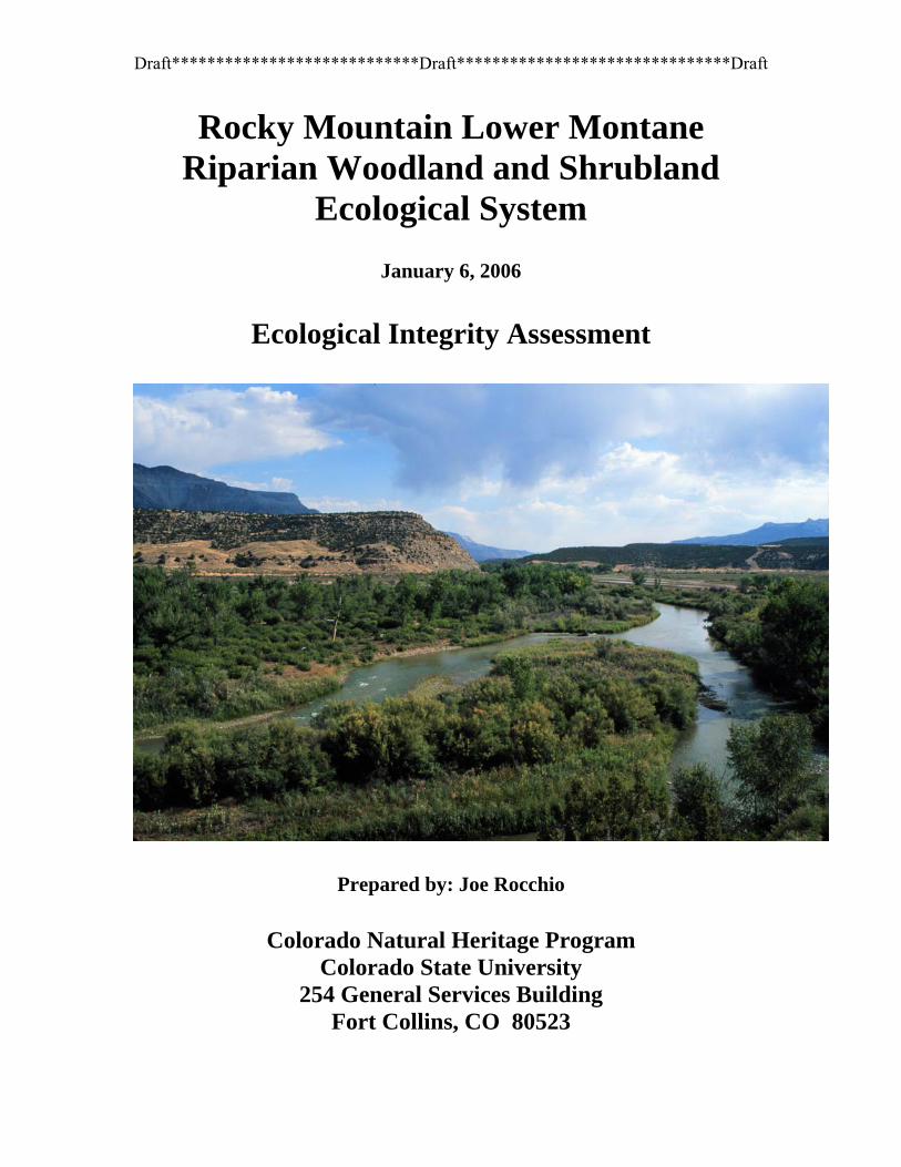
Rocky Mountain Lower Montane Riparian Woodland and Shrubland
Ecological System
January 6, 2006
Ecological Integrity Assessment
Prepared by: Joe Rocchio
Colorado Natural Heritage Program Colorado State University
254 General Services Building Fort Collins, CO 80523

Draft****************************Draft*******************************Draft
TABLE OF CONTENTS
A. INTRODUCTION.................................................................................... 4 A.1 Classification Summary............................................................................................ 4 A.2 Ecological System Description................................................................................. 5
A.2.1. Environment............................................................................................. 5 A.2.2. Vegetation & Ecosystem.......................................................................... 7 A.2.3. Dynamics ................................................................................................. 9 A.2.4. Landscape............................................................................................... 11 A.2.5. Size......................................................................................................... 11
A.3 Ecological Integrity ................................................................................................ 12 A.3.1. Threats.................................................................................................... 12 A.3.2. Justification of Metrics........................................................................... 13 A.3.3. Ecological Integrity Metrics................................................................... 14
A.4 Scorecard Protocols ............................................................................................... 26 A.4.1. Landscape Context Rating Protocol....................................................... 26 A.4.2. Biotic Condition Rating Protocol........................................................... 27 A.4.3 Abiotic Condition Rating Protocol ......................................................... 28 A.4.4 Size Rating Protocol................................................................................ 28 A.4.5 Overall Ecological Integrity Rating Protocol.......................................... 29
B. PROTOCOL DOCUMENTATION FOR METRICS........................ 31 B.1 Landscape Context Metrics .................................................................................... 31
B.1.1. Adjacent Land Use ................................................................................. 31 B.1.2. Buffer Width .......................................................................................... 32 B.1.3. Percentage of Unfragmented Landscape Within One Kilometer........... 33 B.1.4. Riparian Corridor Continuity ................................................................. 34
B.2. Biotic Condition Metrics ....................................................................................... 36 B.2.1. Percent of Cover of Native Plant Species .............................................. 36 B.2.2. Floristic Quality Index (Mean C) ........................................................... 37 B.2.3. Biotic/Abiotic Patch Richness................................................................ 38 B.2.4. Interspersion of Biotic/Abiotic Patches.................................................. 39 B.2.5. Saplings/seedlings of Native Woody Species ........................................ 40
B.3 Abiotic Condition Metrics ...................................................................................... 41 B.3.1 Land Use Within the Wetland................................................................. 41 B.3.2. Sediment Loading Index ........................................................................ 43 B.3.3. Upstream Surface Water Retention........................................................ 44 B.3.4. Upstream/Onsite Water Diversions........................................................ 45 B.3.5. Floodplain Interaction ............................................................................ 47 B.3.6. Surface Water Runoff Index .................................................................. 48 B.3.7. Index of Hydrological Alteration ........................................................... 49 B.3.8. Bank Stability......................................................................................... 50 B.3.9. Beaver Activity ...................................................................................... 51 B.3.10. Litter Cover .......................................................................................... 52 B.3.11. Nutrient/Pollutant Loading Index......................................................... 53 B.3.12. Nutrient Enrichment (C:N)................................................................... 54
ii
Draft****************************Draft*******************************Draft
B.3.13. Nutrient Enrichment (C:P) ................................................................... 56 B.3.14. Soil Organic Matter Decomposition .................................................... 57 B.3.15. Soil Organic Carbon............................................................................. 59 B.3.16. Soil Bulk Density ................................................................................. 60
B.4 Size Metrics ............................................................................................................ 62 B.4.1. Absolute Size.......................................................................................... 62 B.4.2. Relative Size........................................................................................... 63
C. REFERENCES....................................................................................... 65 APPENIDX A: FIELD FORMS............................................................... 74 APPENDIX B: SUPPLEMENTARY DATA:......................................... 80
List of Tables
Table 1. Overall Set of Metrics for the Rocky Mountain Lower Montane Riparian Woodland and Shrubland System. .......................................................................... 15
Table 2. Metric Ranking Criteria. . .................................................................................. 17 Table 3. Landscape Context Rating Calculation.............................................................. 26 Table 4. Biotic Condition Rating Calculation.................................................................. 27 Table 5. Abiotic Condition Rating Calculation. .............................................................. 28 Table 6. Size Rating Calculation. ..................................................................................... 29 Table 7. Current Land Use and Corresponding Land Use Coefficients .......................... 32 Table 8. Biotic/Abiotic Patch Types in Fens ................................................................... 39 Table 9. Current Land Use and Corresponding Land Use Coefficients .......................... 42
iii

Draft****************************Draft*******************************Draft
A. INTRODUCTION
A.1 Classification Summary CES306.821 Rocky Mountain Lower Montane Riparian Woodland and Shrubland Division 306, Woody Wetland Spatial Scale & Pattern: Linear Classification Confidence: medium Required Classifiers: Natural/Semi-natural, Vegetated (>10% vasc.), Wetland Diagnostic Classifiers: Montane [Lower Montane], Mineral: W/ A Horizon <10 cm, Unconsolidated, Short (50-100 yrs) Persistence, Riverine / Alluvial, Short (<5 yrs) Flooding Interval Non-Diagnostic Classifiers: Forest and Woodland (Treed), Shrubland (Shrub-dominated), Braided channel or stream, Drainage bottom (undifferentiated), Floodplain, Stream terrace (undifferentiated), Valley bottom, Temperate [Temperate Continental], Circumneutral Water HGM: Riverine Concept Summary: This system is found throughout the region within a broad elevation range from approximately 900 to 2,800 m. This system often occurs as a mosaic of multiple communities that are tree dominated with a diverse shrub component. This system is dependent on a natural hydrologic regime especially annual to episodic flooding. Occurrences are found within the flood zone of rivers, on islands, sand or cobble bars, and immediate stream banks. They can form large, wide occurrences on mid-channel islands in larger rivers or narrow bands on small, rocky canyon tributaries and well-drained benches. The system is also typically found in backwater channels and other perennial wet, but less scoured sites, such as floodplains swales and irrigation ditches. Dominant trees may include box elder (Acer negundo), narrowleaf cottonwood (Populus angustifolia), balsam poplar (P. balsamifera), plains cottonwood (P. deltoides), Fremont’s cottonwood (P. fremontii), Douglas fir (Pseudotsuaga menziesii), blue spruce (Picea pungens), peachleaf willow (Salix amygdaloides), or Rocky Mountain juniper (Juniperus scopulorum). Dominant shrubs include Rocky Mountain maple (Acer glabrum), thinleaf alder (Alnus incana), river birch (Betula occidentalis), red-osier dogwood (Cornus sericea), river hawthorn (Crataegus rivularis), stretchberry (Forestiera pubescens), chokecherry (Prunus virginiana), skunkbush (Rhus trilobata), mountain willow (Salix monticola), Drummond’s willow (S. drummondiana), narrowleaf willow (S. exigua), dewystem willow (S. irrorata), Pacific willow (S. lucida), buffaloberry (Shepherdia argentea), or snowberry (Symphoricarpos spp.). Exotic trees such as Russian olive (Elaeagus angustifolia) and tamarisk (Tamarix spp.) are common in some stands. The upland vegetation surrounding this riparian system varies and ranges from grasslands to forests. Ecological Divisions (Bailey): 304, 306
4
Draft****************************Draft*******************************Draft
TNC Ecoregions: 11:C, 18:C, 19:C, 20:C, 21:C, 25:C, 6:P, 8:C, 9:C Subnations/Nations: AZ:c, CO:c, ID:c, MT:c, NM:c, NV:c, OR:c, SD:c, UT:c, WY:c
A.2 Ecological System Description
A.2.1. Environment Climate A continental climate dominates the Southern Rocky Mountains producing warm, dry summers and cold winters and an overall semi-arid climate. Most precipitation occurs as snowfall (as much as 80% at high elevations) during the winter months and thus is the most important source of water for wetlands and riparian areas in the Southern Rocky Mountains (Laubhan 2004; Windell et. al 1986; Cooper 1990). However, late-summer convective thunderstorms produce slight peaks in runoff in late summer (Baker 1987; Rink and Kiladis 1986). Evaporation generally exceeds precipitation, especially at lower elevations and in the intermountain basins; however, increasing precipitation and lower temperatures at higher elevations tends to reverse this trend, although aspect, topography, and intense solar radiation can moderate these effects on the evaporation/precipitation ratio (Laubhan 2004). The ratio between evaporation and precipitation has a strong influence on the hydrology of wetlands and riparian areas throughout the region. Climate has a large role in maintenance of riparian areas since the hydrological and geomorphic characteristics of riparian areas are tied to the precipitation and runoff characteristics of their contributing basins. Geomorphology The Southern Rocky Mountains are composed of various igneous, metamorphic, and sedimentary rocks (Mutel and Emerick 1984; Windell et al. 1986). The mountain valleys are relatively young topographical forms created by the erosional effects of flowing water and glacier movement (Windell et al. 1986). Intermountain basins were formed from tectonic and volcanic events which occurred during mountain-forming processes (Windell et al. 1986). The valleys of these basins are now filled with deep alluvial deposits derived from erosional processes in the nearby mountain ranges (Windell et al. 1986). Glaciation has had a large influence on landforms at high elevations through large-scale erosional and depositional processes. Hydrology The interaction of climate and geomorphology has a strong influence on local hydrological processes in a riparian area. For example, snowmelt at high elevations contributes a large proportion of water to most wetland and riparian types through its influence on groundwater and surface water dynamics (Laubhan 2004). In mountain valleys, snowmelt and geomorphology are major factors controlling the extent, depth, and duration of saturation resulting from high groundwater levels and also exert controls most aspects of the frequency, timing, duration, and depth of flooding along riparian areas (Laubhan 2004). Wetlands and riparian areas in intermountain basins are also affected by snowmelt via its association with the contributing surface water to the valley aquifers.
5
Draft****************************Draft*******************************Draft
Flooding from the stream channel recharges many alluvial aquifers and as stream flow decreases the trend is reversed as the alluvial aquifer begins to recharge stream flow (Hubert 2004). Groundwater levels in riparian areas are dependent on the underlying bedrock, watershed topography, soil characteristics, and season (Rink and Kiladis 1986). In areas of thin soils, little surface water is retained as groundwater; however, in areas of deep alluvial material surface water collects in alluvial aquifers which support numerous wetlands (Rink and Kiladis 1986). The level of the water table in alluvial aquifers varies temporally and spatially depending on the distance from the stream channel, time since streamflow has increased or decreased (or flooded), geometry of the river valley, and the composition of the alluvium (Hubert 2004). The temporal and spatial variation of the level of the alluvial aquifer is an important determining factor in the distribution and types of riparian habitats present (Hubert 2004). Surface water flow and flooding is a function of snowmelt, watershed and valley topography and area, late-summer rainfall, and the extent of upstream riparian wetlands (Rink and Kiladis 1986). For example, riparian areas which are steep are not prone to as much flooding as riparian areas in more gently sloped and broad valleys (Mitsch and Gosselink 2000). Watershed area also affects surface flow which has subsequent effects on channel dimensions and varies according to stream discharge, which generally increases with increasing drainage basin area. Baker (1989) notes that in Western Colorado, montane and subalpine streams typically have mean discharges < 71 m3 sec-1 and that historic peak discharges are less than 990 m3 sec-1, which are small for similar sized basins in other areas. Upstream wetlands release water throughout the growing season and are an important contribution to streamflow during later-summer and/or drought periods. Surface water is a very important formative process in riparian areas. Flooding inundates vegetation, can physically dislodge seedlings/saplings, and alter channel morphology through erosion and deposition of sediment. Infrequent, high-powered floods determine large geomorphic patterns that persist on the landscape for hundreds to thousands of years (Hubert 2004). Floods of intermediate frequency and power produce floodplain landforms which persist for tens to hundreds of years while high frequency low-powered floods which occur nearly annually determine short-term patterns such as seed germination and seedling survival (Hubert 2004). Flooding in subalpine-montane streams occurs annually in May and June with the volume and duration affected by snowpack levels (Baker 1987). Occasional September flooding may occur due to intense convective thunderstorms, however these are often very localized (Baker 1987). These thunderstorms can result in sporadic and frequent small-scale flooding in small mountain streams (Hubert 2004). Interannual variation of streamflow can range from 60-150% of the mean annual flow on the west slope, whereas eastern slope streams have less variation (Baker 1987). Runoff from adjacent hillsides can also contribute to the hydrological regime of riparian shrublands by recharging local alluvial aquifers and supporting wetland vegetation that is otherwise disconnected from stream flow (Cooper 1990).
6
Draft****************************Draft*******************************Draft
Riparian areas can generally be referred to as confined or unconfined streams. Gregory et al. (1991) have defined confined streams as those whose valley floors are less than twice the width of the active stream channel. Confined streams typically have relatively straight, single channels flowing through narrow valley floors (Gregory et al. 1991). Flooding in confined streams increases stream depth and flow velocity increases rapidly as discharge increases due to minimal lateral floodplain areas (Gregory et al. 1991). Confined streams typically have shallow soils with minimal alluvium deposition (Hubert 2004). Unconfined streams lack lateral constraint and are typically found in low-gradient, lowland areas or in glaciated valleys and intermountain basins in the mountainous regions. Meandering occurs in unconfined streams where the gradient is low (Hubert 2004). The meander process leads to the formation of a complexity of geomorphic surfaces which support a diverse array of riparian habitats such as point bars, oxbows and backchannels, natural levees, ridges and swales, and pools and riffles in the stream channel, etc. (Hubert 2004; Gregory et al. 1991). These geomorphic surfaces support many different type of vegetation communities such as early seral plant communities, emergent vegetation associated with oxbows and backwater areas, decadent stands of vegetation (Hubert 2004; Gregory et al. 1991). Due to the diversity of abiotic and biotic patches created by the meander process, perennial, low-gradient streams support the most extensive riparian habitat in the Intermountain West (Hubert 2004). Lower Montane Riparian Woodlands and Shrublands are found along confined as well as unconfined streams and are found below the extent of glaciation in the Southern Rocky Mountains. Lower montane riparian areas achieve their most extensive development in the intermountain basins located between mountain ranges (Windell et. al. 1986). However, wide mountain valleys throughout the lower montane zone also support extensive riparian vegetation. Beaver are also an important hydrogeomorphic variable in Rocky Mountain Lower Montane Riparian Woodlands and Shrublands and are discussed below.
A.2.2. Vegetation & Ecosystem Vegetation This system consists of temporarily, seasonally and intermittently flooded woodlands and shrublands comprised of broad leaved deciduous species, both in the tree and shrub canopy, as well as occasional conifers. Species such as Rio Grande cottonwood (Populus deltoides ssp. wislizenii), narrowleaf cottonwood (P. angustifolia), plains cottonwood (P. deltoides ssp. monilifera), Fremont’s cottonwood (P. fremontii), skunkbrush, and narrowleaf willow are common. Other woody species that may be present include Douglas fir (Pseudotsuga menziesii) (on north facing slopes of canyon floors), blue spruce, thinleaf alder (Alnus incana), rockspirea (Holodiscus dumosus), and roundleaf snowberry (Symphoricarpos rotundifolius), western snowberry (Symphoricarpos occidentalis), river birch (Betula occidentalis), Colorado barberry (Berberis fendleri), box elder (Acer negundo), subalpine fir (Abies lasiocarpa), golden currant (Ribes aureum), buffaloberry (Shepherdia argentea), poison ivy (Toxicodendron radicans),
7
Draft****************************Draft*******************************Draft
Wood’s rose (Rosa woodsii), spearleaf rabbitbrush (Chrysothamnus linifolius), stretchberry (Forestiera pubescens) and a variety of willows (Salix spp.). The herbaceous layer is relatively sparse and is typically graminoid dominated. Associated species may include mountain rush (Juncus balticus var. montanus), common spikerush (Eleocharis palustris, saltgrass (Distichlis spicata), wildrye (Elymus spp.), horsetail (Equisetum spp.), foxtail barley (Hordeum jubatum), bulrush (Schoenoplectus spp.), scratchgrass (Muhlenbergia asperifolia), western wheatgrass (Pascopyrum smithii), giant reed (Phragmites australis), Canada goldenrod (Solidago canadensis), starry false lily of the valley (Maianthemum stellatum), sedges (Carex spp.), and various non-native graminoids. The understory may be associated with bare soil, gravel, cobbles, and boulders. Biogeochemistry Bedrock geology, soil characteristics, and discharge of the contributing watershed basin determine the type and amount of nutrient flux in riparian woodland (Windell et al. 1986). Nutrient concentrations in high elevation streams in Colorado tend to be nutrient poor and are related to stream flow (Knud-Hansen 1986). Further downstream, bedrock geology has a large influence on nutrients in stream water. For example, thin coarse soils associated with granitic bedrock are nutrient poor and tend to be acidic whereas soils derived from limestone or shale outcrops have more nutrients and a higher pH (Knud-Hansen 1986). Groundwater can also contribute nutrients via subsurface hillside runoff into riparian areas (Cooper 1990). Periodic flooding is an important contributor of nutrients to riparian areas as it deposits organic material and fine-sediment (Hubert 2004). Riparian areas may serve as important biogeochemical filters of nutrients and sediment before they enter the stream from adjacent human land uses (Peterjohn and Correll 1984). For example, unconfined riparian areas have been shown to retain more than two times the amount of NH4
+ than confined riparian areas (e.g., Rocky Mountain Subalpine-Montane Riparian Woodlands) (Gregory et al. 1991). In Colorado, a 10 m riparian wet meadow buffer zone was experimentally shown to reduce applied NO3
- by 84% and PO4-3
by 79% (Corley et al. 1999). Riparian areas are also important nutrient sources as they provide sources of particulate and dissolved carbon (e.g., detritus) to the stream which are crucial food sources for aquatic invertebrates in local environments as well as downstream areas (Gregory et al. 1991; Kattelmann and Embury 1996). Productivity In general, productivity in terrestrial environments tends to decline with increasing elevation and aridity (Manley and Schlesinger 2001). Because riparian areas contain perennial or intermittent water, they often have higher primary productivity than adjacent upland systems, especially in the semi-arid portions of the Southern Rocky Mountains, and thus have been suggested to be the most productive and diverse parts of the western
8
Draft****************************Draft*******************************Draft
landscape (Gregory et al. 1991; Kattelmann and Embury 1996; Knud-Hansen 1986). In addition, species richness of montane and subalpine riparian areas in the Southern Rocky Mountains was found to be as rich or richer than riparian ecosystems in the southwest, central, and northeast portions of the United States and was found to have higher species richness than most temperate North American forests (Baker 1990). In Colorado, Baker (1990) found that species richness was highest in subalpine riparian forests (mean of 57.8 species/0.1 ha) on the West Slope while Peet (1978) found that montane riparian forests on the East Slope was highest (mean of 60.3 species/0.1 ha). Undisturbed montane riparian forests on the West Slope had an average of 47.4 species/0.1 ha (Baker 1990). The spatial complexity of patch types in the riparian zone results in a high edge-area ratio creating many ecotones with contrasting environmental processes and habitat types (Knud-Hansen 1986; Manley and Schlesinger 2001). This spatial heterogeneity supports numerous types of plant communities which provide for abundant secondary productivity of riparian areas (i.e. abundant support of fauna taxa). Riparian vegetation also shades streamside aquatic habitat and therefore regulates stream temperatures which as large implications on habitat quality for aquatic invertebrates and fish. Animals The spatial complexity of riparian areas support numerous vegetation types such wet meadows and marshes. These community types are associated with the Lower Montane Riparian Woodland and Shrubland system, unless they are large enough (i.e., meet the minimum size criteria) to classify as another Ecological System types (e.g., Rocky Mountain Alpine-Montane Wet Meadows or North American Arid Freshwater Marsh). These communities have their own unique assemblages of plants which in turn support a variety of aquatic and terrestrial invertebrates. These invertebrates process detritus, consume vegetation, and provide abundant food resources for other taxa such as birds, mammals, fish, amphibians, and other invertebrate species. In the Sierra Nevada Mountains, approximately 400 species of vertebrates are dependent on riparian areas for a portion of their life cycle (Kattelmann and Embury 1996). In Colorado, it is estimated that riparian areas, which account for only 1% of the landscape, are used by greater than 70% of the state’s wildlife species and 27% of the breeding bird species depend on riparian habitats for their viability (Knopf 1988; Pague and Carter 1996). Deer, moose, and elk seek out riparian shrublands and wet meadows for their rich and nutritious grasses and forbs (Foster 1986). Lower montane riparian areas are also important for variety of native fish, including native cutthroat trout (Windell et al. 1986). Open water areas such as beaver ponds provide nesting, feeding, and resting habitat for migrating waterbirds (Foster 1986). Small mammals such as meadow voles (Microtus pennsylvanicus), pocker gophers (Thomomys talpoides), field mice (Permyscus spp.), shrews (Sorex spp.), mink (Mustela vison), and ground squirrels (Citellus spp.) may use riparian woodlands that are seasonally wet (Foster 1986).
A.2.3. Dynamics Development of lower montane riparian areas is driven mostly by the magnitude and frequency of flooding, valley type, and beaver activity. Seasonal and episodic flooding
9

Draft****************************Draft*******************************Draft
erode and/or deposit sediment resulting in complex patterns of soil development which subsequently have a strong influence on the distribution of riparian vegetation (Gregory et al. 1991; Poff et al. 1997). Bare alluvium also provides suitable substrate for the germination of cottonwood and willow seedlings and is thus a critical patch type for continued regeneration of riparian vegetation (Poff et al. 1997; Woods 2001). Alluvial soils are of variable thickness and texture and often exhibit redoximorphic features such as mottling, indicating a fluctuating water table. Valley geomorphology, flooding regime, and substrate dictate the types of riparian vegetation which develops. For example, this ecological system contains early seral, mid- and late seral riparian plant associations as well as a diversity of wet meadow and emergent wetland communities. The distribution and extent of these communities is determined by valley type (confined vs. unconfined), flooding regime, and beaver activity. Cottonwood communities are early, mid- or late seral, depending on the age class of the trees and the associated species of the stand (Kittel et al. 1998). Mature cottonwood stands do not regenerate in place, but regenerate by “moving” up and down a river reach by establishing on “new ground” created by seasonal and episodic flooding. Overtime a healthy riparian area supports all stages of cottonwood communities (Kittel et al. 1998). Narrowleaf willow (Salix exigua) persists under a regime of repeated fluvial disturbances and is an early seral plant species. Narrowleaf willow is often found with cottonwood seedlings and overtime may succeed to a cottonwood dominated community type. As cottonwood forests mature, they become more disconnected from the stream, mostly due to changes in channel migration and morphology, and are often found on secondary floodplain terraces. Blue spruce (Picea pungens) may establish in mature and decadent cottonwood forests in higher elevations, while species such skunkbush (Rhus trilobata) is a late seral riparian species found within this system at lower elevations (i.e. along the Colorado River near Grand Junction). Beavers typically inhabit streams with a gentle gradient (< 15%) and in wide valleys (at least wider than the stream channel) (Bierly 1972). Beaver dams impound surface water creating open water areas. When dams are initially created, they often flood and kill large areas of shrublands or trees. These areas are eventually colonized by herbaceous emergent and submergent vegetation. As local food supplies are diminished, beavers tend to abandon their dams and move up or downstream to find additional food supply as well as suitable dam sites (Baker 1987; Phillips 1977). The abandoned beaver ponds eventually fill with sediment and are colonized by willows and saplings, thus completing the cycle. The presence of beaver creates a heterogeneous complex of wet meadows and riparian shrublands and increases species richness on the landscape. For example, Wright et al. (2002) note that beaver-modified areas may contribute as much as 25% of the species richness of herbaceous species in Adirondack Mountains of New York. Naiman et al. (1986) note that beaver-influenced streams are very different from those not impacted by beaver activity by having numerous zones of open water and vegetation, large accumulations of detritus and nutrients, more wetland areas, having more anaerobic biogeochemical cycles, and in general are more resistance to disturbance. Neff (1957; in Knight 1994) estimated that a Colorado valley with an active beaver colony had eighteen
10
Draft****************************Draft*******************************Draft
times more water storage in the spring and an ability to support higher streamflow in late summer than a drainage where beaver were removed. It is not known what the density of beaver were in the Southern Rocky Mountains prior to the fur trade (Baker 1987); however, Naiman et al. (1986) suggest that when beaver are not managed or harvested their activity may influence 20-40% of the total length of 2nd to 5th order streams in the boreal forest of Canada. It is apparent that active beaver colonies are very important for ecosystem development in riparian areas.
A.2.4. Landscape It is evident from the hydro-geomorphic setting of lower montane riparian shrublands that their integrity is partly determined by processes operating in the surrounding landscape and more specifically in the contributing watershed. The quality and quantity of ground and surface water input into riparian areas is almost entirely determined by the condition of the surrounding landscape. Various types of land use can alter surface runoff, recharge of local aquifers, and introduce excess nutrients, pollutants, or sediments. Riparian areas are intimately connected to uplands in their upstream watersheds as well as adjacent areas. However, the reverse is also true: riparian areas provide connectivity between upland systems and between up and downstream riparian patch types (Wiens 2002). Thus, the types, abundance, and spatial distribution of riparian patch types is an important ecological component to these systems as they affect the flow and movement of nutrients, water, seed dispersal, and animal movement (Wiens 2002). Assessments of riparian areas have considered the landscape properties of the local watershed to be a critical factor in assessing condition (Hauer et al. 2002, Hauer and Smith 1998, Costick 1996, Moyle and Randall 1998, Richter et al. 1996, Poff et al. 1997, and Rondeau 2001).
A.2.5. Size The size of a wetland or riparian area, whether very small or very large, is a natural characteristic defined by a site’s topography, soils, and hydrological processes. The natural range of sizes found on the landscape varies for each wetland type. As long as a wetland has not been reduced in size by human impacts or isn’t surrounded by areas which have experienced human disturbances, then size isn’t very important to the assessment of ecological integrity. However, if human disturbances have decreased the size of the wetland or if the surrounding landscape is impacted and has the potential to affect the wetland, larger sized wetlands are able to buffer against these impacts better than smaller sized wetlands due to the fact they generally possess a higher diversity of abiotic and biotic processes allowing them to recover and remain more resilient. Under such circumstances, size may be an important factor in assessing ecological integrity. Size is often very important when the conservation or functional value of a wetland is considered. For example, larger wetlands tend to have more diversity, often support
11
Draft****************************Draft*******************************Draft
larger populations of component species, are more likely to support sparsely distributed species, and may provide more suitable wildlife habitat as well as more ecological services derived from natural ecological processes (e.g. sediment/nutrient retention, floodwater storage, etc.) than smaller wetlands. Thus, when conservation or functional values are of concern, size is almost always an important component to the assessment. Of course, in the context of regulatory wetland mitigation, size is always important whether mitigation transactions are based on function or integrity “units” and thus should be used to weight such transactions. The size of riparian shrublands can vary greatly depending on their topographic location, underlying soil texture, and driving hydrological processes. Some are very small (> 8 linear km) while others can be very large (< 1.5 linear km).
A.3 ECOLOGICAL INTEGRITY
A.3.1. Threats Hydrological Alteration: Reservoirs, water diversions, ditches, roads, and human land uses in the contributing watershed can have a substantial impact on the hydrology as well as biotic integrity of riparian areas (Woods 2001; Kattelmann and Embury 1996; Poff et al. 1997; Baker 1987). All these stressors can induce downstream erosion and channelization, reduce changes in channel morphology, reduce base and/or peak flows, lower water tables in floodplains, and reduce sediment deposition in the floodplain (Poff et al. 1997). Vegetation responds to these changes by shifting from wetland and riparian dependent species to more mesic and xeric species typical of adjacent uplands and/or encroaching into the stream channel. Without periodic disturbance by flooding, riparian areas become dominated by late-seral communities due to the inability of pioneer species (e.g., cottonwood and willow) to regenerate. These late-seral communities are dominated by more upland species, such as conifers in montane areas or other, more drought tolerant species in the foothill and plains environments (Kittel et al 1998). Floodplain width and the abundance and spatial distribution of various patch types also typically decline. In addition, the spatial complexity of riparian and wetland habitat is greatly reduced due to alteration of the flooding regime. An unaltered hydrologic regime is crucial to maintaining the diversity and viability of the riparian area. Nutrient enrichment: Adjacent and upstream land uses all have the potential to contribute excess nutrients into riparian areas. Increased nutrients can alter species composition by allowing aggressive, invasive species to displace native species. Altered hydrology can disrupt nutrient cycles by eliminating normal flushing cycles and lack of deposition of organic material from floodwaters. Exotics: Non-native plants or animals can have wide-ranging impacts. Non-native plants can increase dramatically under the right conditions and essentially dominate a previously natural area. This can generate secondary effects on animals (particularly
12

Draft****************************Draft*******************************Draft
invertebrates) that depend on native plant species for forage, cover, or propagation. Tamarisk (Tamarix spp.) and Russian olive (Elaeagnus angustifolia) are two aggressive non-native shrubs which can invade and drastically alter ecological processes in lower montane riparian areas. Tamarisk can decrease the amount of sediment deposition in floodplains, displace native vegetation, alter nutrient cycles due to the excessive salts it contributes to the soil, and stabilize streambanks reducing the connectivity between the river and floodplain areas (Graf 1978; Sala 1996). Unfortunately, tamarisk can be extremely difficult to eradicate. Other common aggressive non-native species in the lower montane riparian zone are tumble mustard (Sisymbrium altissimum), Canada thistle (Cirsium canadensis), Russian knapweed (Acroptilon repens), alfalfa (Medicago sativa), sweet clover (Melilotus alba; M. officinalis), reedcanary grass (Phalaris arundinacea), barnyard grass (Echinochloa crus-galli), cocklebur (Xanthium strumarium), red top (Agrostis gigantea), and Kentucky bluegrass (Poa pratensis). Fragmentation: Human land uses both within the riparian area as well as in adjacent and upland areas can fragment the landscape and thereby reduce connectivity between riparian patches and between riparian and upland areas. This can adversely affect the movement of surface/groundwater, nutrients, and dispersal of plants and animals. Roads, bridges, and development can also fragment both riparian and upland areas. Intensive grazing and recreation can also create barriers to ecological processes.
A.3.2. Justification of Metrics As reviewed above, the literature suggests that the following attributes are important measures of the ecological integrity of Rocky Mountain Lower Montane Riparian Woodland and Shrublands:
Landscape Context: Land use within the contributing watershed and riparian corridor has important effects on the connectivity and sustainability of many ecological processes critical to this system.
Biotic condition: Species composition and diversity, presence of conservative plants, regeneration, and invasion of exotics are important measures of biological integrity.
Abiotic Condition: Hydrological integrity is the most important variable to measure, however land use within the wetland can have detrimental impacts on other important abiotic processes such as nutrient cycling, bank stability, and floodplain interaction.
Size: Absolute size is important for consideration of conservation values as well as ecosystem resilience. Relative size is also very important as it provides information regarding historical loss or degradation of wetland size.
13
Draft****************************Draft*******************************Draft
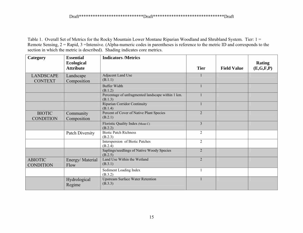
A.3.3. Ecological Integrity Metrics A synopsis of the ecological metrics and ratings is presented in Table 2. The three tiers refer to levels of intensity of sampling required to document a metric. Tier 1 metrics are able to be assessed using remote sensing imagery, such as satellite or aerial photos. Tier 2 typically require some kind of ground sampling, but may require only qualitative or semi-quantitative data. Tier 3 metrics typically require a more intensive plot sampling or other intensive sampling approach. A given measure could be assessed at multiple tiers, though some metrics are not doable at Tier 1 (i.e., they require a ground visit). Core and Supplementary Metrics The Scorecard (see Tables 1 & 2) contains two types of metrics: Core and Supplementary. Separating the metrics into these two categories allows the user to adjust the Scorecard to available resources, such as time and funding, as well as providing a mechanism to tailor the Scorecard to specific information needs of the user. Core metrics are shaded gray in Tables 1 & 2 and represent the minimal metrics that should be applied to assess ecological integrity. Sometimes, a Tier 3 Core metric might be used to replace Tier 2 Core Metrics. For example, if a Vegetation Index of Biotic Integrity is used, then it would not be necessary to use similar Tier 2 Core metrics such as Percentage of Native Graminoids, Percentage of Native Plants, etc. Supplementary metrics are those which should be applied if available resources allow a more in depth assessment or if these metrics add desired information to the assessment. Supplementary metrics are those which are not shaded in Tables 1 & 2.
14
Draft****************************Draft*******************************Draft
Table 1. Overall Set of Metrics for the Rocky Mountain Lower Montane Riparian Woodland and Shrubland System. Tier: 1 = Remote Sensing, 2 = Rapid, 3 =Intensive. (Alpha-numeric codes in parentheses is reference to the metric ID and corresponds to the section in which the metric is described). Shading indicates core metrics.
Category EssentialEcological Attribute
Indicators /Metrics
Tier
Field Value
Rating
(E,G,F,P)
LANDSCAPE CONTEXT
Landscape Composition
Adjacent Land Use (B.1.1)
1
Buffer Width (B.1.2)
1
Percentage of unfragmented landscape within 1 km. (B.1.3)
1
Riparian Corridor Continuity (B.1.4)
1
BIOTIC CONDITION
Community Composition
Percent of Cover of Native Plant Species (B.2.1)
2
Floristic Quality Index (Mean C) (B.2.2)
3
Patch Diversity Biotic Patch Richness (B.2.3)
2
Interspersion of Biotic Patches (B.2.4)
2
Saplings/seedlings of Native Woody Species (B.2.5)
2
ABIOTIC CONDITION
Energy/ Material Flow
Land Use Within the Wetland (B.3.1)
2
Sediment Loading Index (B.3.2)
1
Hydrological Regime
Upstream Surface Water Retention (B.3.3)
1
15

Draft****************************Draft*******************************Draft
Category Essential Ecological Attribute
Indicators /Metrics
Tier
Field Value
Rating
(E,G,F,P)
Upstream/Onsite Water Diversions (B.3.4)
1
Floodplain Interaction (B.3.5)
2
Surface Water Runoff Index (B.3.6)
1
Index of Hydrological Alteration (B.3.7) NOTE: this metric should be used in lieu of B.3.3, B.3.4, B.3.5 and B.3.6 when data are available.
3
Bank Stability (B.3.8)
2
Beaver Activity (B.3.9)
2
Chemical/Physical Processes
Litter Cover (B.3.10)
2
Nutrient/ Pollutant Loading Index (B.3.11)
1
Nitrogen Enrichment (C:N) (B.3.12)
3
Phosphorous Enrichment (C:P) (B.3.13)
3
Soil Organic Matter Decomposition (B.3.14)
2
Soil Organic Carbon (B.3.15)
3
Soil Bulk Density (B.3.16)
3
SIZE Absolute Size Absolute Size (B.4.1) 1 Relative Size Relative Size (B.4.2) 1
16
Draft****************************Draft*******************************Draft
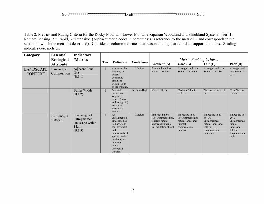
Table 2. Metrics and Rating Criteria for the Rocky Mountain Lower Montane Riparian Woodland and Shrubland System. Tier: 1 = Remote Sensing, 2 = Rapid, 3 =Intensive. (Alpha-numeric codes in parentheses is reference to the metric ID and corresponds to the section in which the metric is described). Confidence column indicates that reasonable logic and/or data support the index. Shading indicates core metrics.
Category Metric Ranking Criteria
Essential Ecological Attribute
Indicators /Metrics
Tier
Definition
Confidence Excellent (A) Good (B) Fair (C) Poor (D)
LANDSCAPE CONTEXT
Landscape Composition
Adjacent Land Use (B.1.1)
1 Addresses the intensity of human dominated land uses within 100 m of the wetland.
Medium Average Land Use Score = 1.0-0.95
Average Land Use Score = 0.80-0.95
Average Land Use Score = 0.4-0.80
Average Land Use Score = < 0.4
Buffer Width (B.1.2)
1 Wetland buffers are vegetated, natural (non-anthropogenic) areas that surround a wetland.
Medium/High Wide > 100 m Medium. 50 m to <100 m
Narrow. 25 m to 50 m
Very Narrow. < 25 m
Landscape Pattern
Percentage of unfragmented landscape within 1 km. (B.1.3)
1 An unfragmented landscape has no barriers to the movement and connectivity of species, water, nutrients, etc. between natural ecological systems.
Medium Embedded in 90-100% unfragmented, roadless natural landscape; internal fragmentation absent
Embedded in 60-90% unfragmented natural landscape; internal fragmentation minimal
Embedded in 20-60%% unfragmented natural landscape; Internal fragmentation moderate
Embedded in < 20% unfragmented natural landscape. Internal fragmentation high
17

Draft****************************Draft*******************************Draft
Category Metric Ranking Criteria
Essential Ecological Attribute
Indicators /Metrics
Tier
Definition
Confidence Excellent (A) Good (B) Fair (C) Poor (D)
Riparian Corridor Continuity (B.1.4)
1 Indicates the degree to which the riparian area exhibits an uninterrupted vegetated riparian corridor.
Medium/High < 5% of riparian reach with gaps / breaks due to cultural alteration
> 5 - 20% of riparian reach with gaps / breaks due to cultural alteration
>20 - 50% of riparian reach with gaps / breaks due to cultural alteration
> 50% of riparian reach with gaps / breaks due to cultural alteration
BIOTIC CONDITION
Community Composition
Percent of Cover of Native Plant Species (B.2.1)
2 Percent of the plant species which are native to the Southern Rocky Mountains.
High 100% cover of native plant species
85-< 100% cover of native plant species
50-85% cover of native plant species
<50% cover of native plant species
Floristic Quality Index (Mean C) (B.2.2)
3 The mean conservatism of all the native species growing in the wetland.
High Mean C > 4.5 Mean C = 3.5-4.5 Mean C = 3.0 – 3.5 Mean C < 3.0
Community Extent
Biotic/Abiotic Patch Richness (B.2.3)
2 The number of biotic/abiotic patches or habitat types present in the wetland.
Medium > 75-100% of the possible patch types are evident in the wetland
> 50-75% of the possible patch types are evident in the wetland
25-50% of the possible patch types are evident in the wetland
< 25% of the possible patch types are evident in the wetland
18
Draft****************************Draft*******************************Draft
Category Metric Ranking Criteria
Essential Ecological Attribute
Indicators /Metrics
Tier
Definition
Confidence Excellent (A) Good (B) Fair (C) Poor (D)
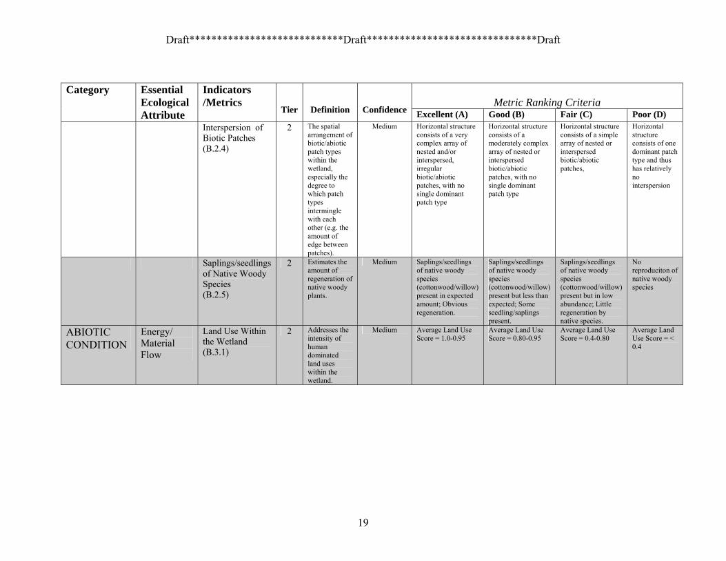
Interspersion of Biotic Patches (B.2.4)
2 The spatial arrangement of biotic/abiotic patch types within the wetland, especially the degree to which patch types intermingle with each other (e.g. the amount of edge between patches).
Medium Horizontal structureconsists of a very complex array of nested and/or interspersed, irregular biotic/abiotic patches, with no single dominant patch type
Horizontal structure consists of a moderately complex array of nested or interspersed biotic/abiotic patches, with no single dominant patch type
Horizontal structure consists of a simple array of nested or interspersed biotic/abiotic patches,
Horizontal structure consists of one dominant patch type and thus has relatively no interspersion
Saplings/seedlings of Native Woody Species (B.2.5)
2 Estimates the amount of regeneration of native woody plants.
Medium Saplings/seedlings of native woody species (cottonwood/willow) present in expected amount; Obvious regeneration.
Saplings/seedlings of native woody species (cottonwood/willow) present but less than expected; Some seedling/saplings present.
Saplings/seedlings of native woody species (cottonwood/willow) present but in low abundance; Little regeneration by native species.
No reproduciton of native woody species
ABIOTIC CONDITION
Energy/ Material Flow
Land Use Within the Wetland (B.3.1)
2 Addresses the intensity of human dominated land uses within the wetland.
Medium Average Land Use Score = 1.0-0.95
Average Land Use Score = 0.80-0.95
Average Land Use Score = 0.4-0.80
Average Land Use Score = < 0.4
19
Draft****************************Draft*******************************Draft
Category Metric Ranking Criteria
Essential Ecological Attribute
Indicators /Metrics
Tier
Definition
Confidence Excellent (A) Good (B) Fair (C) Poor (D)
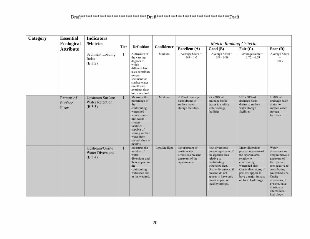
Sediment Loading Index (B.3.2)
1 A measure of the varying degrees to which different land uses contribute excess sediment via surface water runoff and overland flow into a wetland.
Medium Average Score = 0.9 – 1.0
Average Score = 0.8 – 0.89
Average Score = 0.75 – 0.79
Average Score =
< 0.7
Pattern of Surface Flow
Upstream Surface Water Retention (B.3.3)
1 Measures the percentage of the contributing watershed which drains into water storage facilities capable of storing surface water from several days to months
Medium < 5% of drainage basin drains to surface water storage facilities
>5 - 20% of drainage basin drains to surface water storage facilities
>20 - 50% of drainage basin drains to surface water storage facilities
> 50% of drainage basin drains to surface water storage facilities
Upstream/Onsite Water Diversions (B.3.4)
1 Measures the number of water diversions and their impact in the contributing watershed and in the wetland.
Low/Medium No upstream or onsite water diversions present upstream of the riparian area
Few diversions present upstream of the riparian area relative to contributing watershed size. Onsite diversions, if present, do not appear to have only minor impact on local hydrology.
Many diversions present upstream of the riparian area relative to contributing watershed size. Onsite diversions, if present, appear to have a major impact on local hydrology.
Water diversions are very numerous upstream of the riparian area relative to contributing watershed size. Onsite diversions, if present, have drastically altered local hydrology.
20
Draft****************************Draft*******************************Draft
Category Metric Ranking Criteria
Essential Ecological Attribute
Indicators /Metrics
Tier
Definition
Confidence Excellent (A) Good (B) Fair (C) Poor (D)
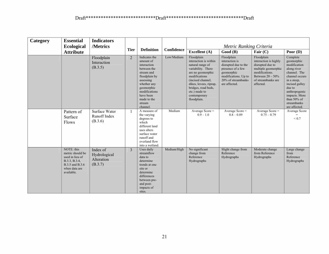
Floodplain Interaction (B.3.5)
2 Indicates the amount of interaction between the stream and floodplain by assessing whether any geomorphic modifications have been made to the stream channel.
Low/Medium Floodplain interaction is within natural range of variability. There are no geomorphic modifications (incised channel, dikes, levees, riprap, bridges, road beds, etc.) made to contemporary floodplain.
Floodplain interaction is disrupted due to the presence of a few geomorphic modifications. Up to 20% of streambanks are affected.
Floodplain interaction is highly disrupted due to multiple geomorphic modifications. Between 20 – 50% of streambanks are affected.
Complete geomorphic modification along river channel. The channel occurs in a steep, incised gulley due to anthropogenic impacts. More than 50% of streambanks are affected.
Pattern of Surface Flows
Surface Water Runoff Index (B.3.6)
1 A measure of the varying degrees to which different land uses alters surface water runoff and overland flow into a wetland.
Medium Average Score = 0.9 – 1.0
Average Score = 0.8 – 0.89
Average Score = 0.75 – 0.79
Average Score =
< 0.7
NOTE: this metric should be used in lieu of B.3.3, B.3.4, B.3.5 and B.3.6 when data are available.
Index of Hydrological Alteration (B.3.7)
3 Uses daily streamflow data to determine trends at one site or determine differences between pre- and post-impacts of sites.
Medium/High No significant change from Reference Hydrographs
Slight change from Reference Hydrographs
Moderate change from Reference Hydrographs
Large change from Reference Hydrographs
21

Draft****************************Draft*******************************Draft
Category Metric Ranking Criteria
Essential Ecological Attribute
Indicators /Metrics
Tier
Definition
Confidence Excellent (A) Good (B) Fair (C) Poor (D)
Bank Stability (B.3.8)
2 Assesses the stability and condition of the streambanks.
Medium Banks stable; evidence of erosion of bank failure absent or minimal; little potential for future problems. < 5% of bank affected. Streambanks dominated (> 90% cover) by Stabilizing Plant Species (OBL & FACW)
Moderately stable; infrequent, small areas of erosion mostly healed over. 5-30% of bank in reach has areas of erosion. Streambanks have 75-90% cover of Stabilizing Plant Species (OBL & FACW)
Moderately unstable; 30-60% of bank in reach has areas of erosion; high erosion potential during floods. Streambanks have 60-75% cover of Stabilizing Plant Species (OBL & FACW)
Unstable; many eroded areas; "raw" AREAS frequent along straight sections and bends; obvious bank sloughing; 60-100% of bank has erosional scars. Streambanks have < 60% cover of Stabilizing Plant Species (OBL & FACW)
Beaver Activity
Beaver Activity (B.3.9)
2 Assesses the presence and degree of beaver activity.
Medium New, recent, and/orold beaver dams present. Beaver currently active in the area.
Recent and old beaver dams present. Beaver may not be currently active but evidence suggests that have been within past 10 years.
Only old beaver dams present. No evidence of recent or new beaver activity despite available food resources and habitat.
Nutrient Cycling
Litter Cover (B.3.10)
2 The percent cover of plant litter or detritus covering the soil surface.
Low/Medium Litter cover 75-125% of Reference Standard (Litter > 50% cover)
Litter cover 25-75% of Reference Standard (Litter 10-50% cover)
Litter cover 0-25% of Reference Standard (Litter cover present but sparse < 10%)
No litter present.
22

Draft****************************Draft*******************************Draft
Category Metric Ranking Criteria
Essential Ecological Attribute
Indicators /Metrics
Tier
Definition
Confidence Excellent (A) Good (B) Fair (C) Poor (D)
Nutrient Enrichment
Nutrient/ Pollutant Loading Index (B.3.11)
1 A measure of the varying degrees to which different land uses contributed excess nutrients and pollutants via surface water runoff and overland flow into a wetland.
Medium Average Score = 0.9 – 1.0
Average Score = 0.8 – 0.89
Average Score = 0.75 – 0.79
Average Score =
< 0.7
Nitrogen Enrichment (C:N) (B.3.12)
3 The carbon to nitrogen (C:N) ratio in the aboveground biomass or leaves of plants. .
Medium/High Leaf tissue C:N is equivalent to natural range of variability
Leaf tissue C:N is slightly less and outside of natural range of variability
Leaf tissue C:N is significantly lower than natural range of variability
Leaf tissue C:N is significantly lower than natural range of variability
Phosphorous Enrichment (C:P) (B.3.13)
3 The carbon to phosphorous (C:P) ratio in the aboveground biomass or leaves of plants.
Medium/High Leaf tissue C:P is equivalent to natural range of variability
Leaf tissue C:P is slightly less and outside of natural range of variability
Leaf tissue C:P is significantly lower than natural range of variability
Leaf tissue C:P is significantly lower than natural range of variability
23

Draft****************************Draft*******************************Draft
Category Metric Ranking Criteria
Essential Ecological Attribute
Indicators /Metrics
Tier
Definition
Confidence Excellent (A) Good (B) Fair (C) Poor (D)
Organic matter
Soil Organic Matter Decomposition (B.3.14)
2 The metric is calculated as an Organic Matter Decomposition Factor (OMDF) based on the depth of the O-horizon, the depth and soil color value of the surface-horizons.
Medium Mature Cottonwoodareas: OMDF > 2.25; Immature cottonwood areas & cottonwood/ willow seedlings: OMDF > 0.8
Mature Cottonwood areas: OMDF 1.1 - 2.25; Immature cottonwood areas & cottonwood/ willow seedlings: OMDF 0.4 - 0.8
Mature Cottonwood areas: OMDF 0.5 - 1.1; Immature cottonwood areas & cottonwood/ willow seedlings: OMDF 0.2 - 0.4
Mature Cottonwood areas: OMDF < 0.5; Immature cottonwood areas & cottonwood/ willow seedlings: OMDF < 0.2
Soil Organic Carbon (B.3.15)
3 Measures the amount of soil organic carbon present in the soil.
Medium/High Soil C is equivalent to natural range of variability
Soil C is nearly equivalent to natural range of variability
Soil C is significantly lower than natural range of variability
Soil C is significantly lower than natural range of variability
Compaction Soil Bulk Density (B.3.16)
3 A measure of the compaction of the soil horizons.
Medium/High Bulk density is within natural range of variability
Bulk density is slightly higher than natural range of variability
Bulk density is higher than natural range of variability
Bulk density is much higher than natural range of variability
SIZE Absolute Size
Absolute Size (B.4.1)
1 The current size of the wetland
High > 8.0 linear km (minimum of 10 m wide)
5.0 to 8.0 linear km (minimum of 10 m wide)
1.5 to 5.0 linear km (minimum of 10 m wide)
< 1.5 linear km (minimum of 10 m wide)
24
Draft****************************Draft*******************************Draft
Category Metric Ranking Criteria
Essential Ecological Attribute
Indicators /Metrics
Tier
Definition
Confidence Excellent (A) Good (B) Fair (C) Poor (D)
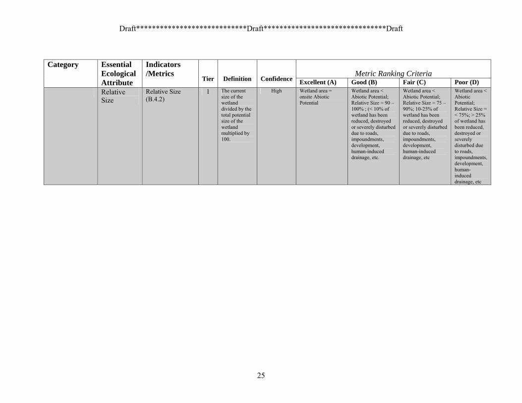
Relative Size
Relative Size (B.4.2)
1 The current size of the wetland divided by the total potential size of the wetland multiplied by 100.
High Wetland area = onsite Abiotic Potential
Wetland area < Abiotic Potential; Relative Size = 90 – 100% ; (< 10% of wetland has been reduced, destroyed or severely disturbed due to roads, impoundments, development, human-induced drainage, etc.
Wetland area < Abiotic Potential; Relative Size = 75 – 90%; 10-25% of wetland has been reduced, destroyed or severely disturbed due to roads, impoundments, development, human-induced drainage, etc
Wetland area < Abiotic Potential; Relative Size = < 75%; > 25% of wetland has been reduced, destroyed or severely disturbed due to roads, impoundments, development, human-induced drainage, etc
25

Draft****************************Draft*******************************Draft
A.4 Scorecard Protocols For each metric, a rating is developed and scored as A – (Excellent) to D – (Poor). The background, methods, and rationale for each metric are provided in section B. Each metric is rated, then various metrics are rolled together into one of four categories: Landscape Context, Biotic Condition, Abiotic Condition, and Size. A point-based approach is used to roll-up the various metrics into Category Scores. Points are assigned for each rating level (A, B, C, D) within a metric. The default set of points are A = 5.0, B = 4.0, C = 3.0, D = 1.0. Sometimes, within a category, one measure is judged to be more important than the other(s). For such cases, each metric will be weighted according to its perceived importance. Points for the various measures are then added up and divided by the total number of metrics. The resulting score is used to assign an A-D rating for the category. After adjusting for importance, the Category scores could then be averaged to arrive at an Overall Ecological Integrity Score. Supplementary metrics are not included in the Rating Protocol. However, they could be incorporated if the user desired.
A.4.1. Landscape Context Rating Protocol Rate the Landscape Context metrics according to their associated protocols (see Table 2 and details in Section B). Use the scoring table below (Table 3) to roll up the metrics into an overall Landscape Context rating. Rationale for Scoring: Adjacent land use, buffer width, and connectivity of the riparian corridor are judged to be more important than the amount of fragmentation within 1 km of the wetland since a wetland with no other natural communities bordering it is very unlikely to have a strong biological connection to other natural lands at a further distance. Thus, the following weights apply to the Landscape Context metrics:
Table 3. Landscape Context Rating Calculation.
Measure Definition Tier A
B
C
D
Weight Score (weight x rating)
Adjacent Land Use (B.1.1)
Addresses the intensity of human dominated land uses within 100 m of the wetland.
1 5 4 3 1 0.30
Buffer Width (B.1.2)
Wetland buffers are vegetated, natural (non-anthropogenic) areas that surround a wetland.
1 5 4 3 1 0.30
Percentage of unfragmented landscape within 1 km. (B.1.3)
An unfragmented landscape has no barriers to the movement and connectivity of species, water, nutrients, etc. between natural ecological systems.
1 5 4 3 1 0.10
26
Draft****************************Draft*******************************Draft
Measure Definition Tier A
B
C
D
Weight Score (weight x rating)
Riparian Corridor Continuity (B.1.4)
Indicates the degree to which the riparian area exhibits an uninterrupted vegetated riparian corridor.
1 5 4 3 1 0.30
Landscape Context Rating
A = 4.5 - 5.0 B = 3.5 – 4.4 C = 2.5 – 3.4 D = 1.0 – 2.4
Total = sum of N scores
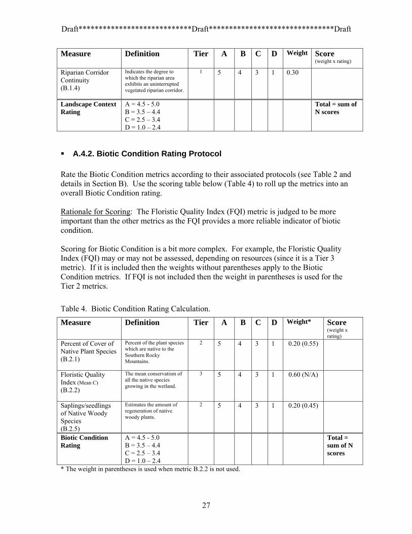
A.4.2. Biotic Condition Rating Protocol Rate the Biotic Condition metrics according to their associated protocols (see Table 2 and details in Section B). Use the scoring table below (Table 4) to roll up the metrics into an overall Biotic Condition rating. Rationale for Scoring: The Floristic Quality Index (FQI) metric is judged to be more important than the other metrics as the FQI provides a more reliable indicator of biotic condition. Scoring for Biotic Condition is a bit more complex. For example, the Floristic Quality Index (FQI) may or may not be assessed, depending on resources (since it is a Tier 3 metric). If it is included then the weights without parentheses apply to the Biotic Condition metrics. If FQI is not included then the weight in parentheses is used for the Tier 2 metrics.
Table 4. Biotic Condition Rating Calculation.
Measure Definition Tier A
B
C
D
Weight* Score (weight x rating)
Percent of Cover of Native Plant Species (B.2.1)
Percent of the plant species which are native to the Southern Rocky Mountains.
2 5 4 3 1 0.20 (0.55)
Floristic Quality Index (Mean C) (B.2.2)
The mean conservatism of all the native species growing in the wetland.
3 5 4 3 1 0.60 (N/A)
Saplings/seedlings of Native Woody Species (B.2.5)
Estimates the amount of regeneration of native woody plants.
2 5 4 3 1 0.20 (0.45)
Biotic Condition Rating
A = 4.5 - 5.0 B = 3.5 – 4.4 C = 2.5 – 3.4 D = 1.0 – 2.4
Total = sum of N scores
* The weight in parentheses is used when metric B.2.2 is not used.
27

Draft****************************Draft*******************************Draft
A.4.3 Abiotic Condition Rating Protocol Rate the Abiotic Condition metrics according to their associated protocols (see Table 2 and details in Section B). Use the scoring table below (Table 5) roll up the metrics into an overall Abiotic Condition rating. Rationale for Scoring: Quantitative water table data are judged to more reliable than the other metrics for indicating Abiotic Condition (shaded metric in Table 5). However, if such data are lacking then stressor related metrics (Land Use & Hydrological Alterations) are perceived to provide more dependable information concerning Abiotic Condition.
Table 5. Abiotic Condition Rating Calculation.
Measure Definition Tier A
B
C
D
Weight* Score (weight x rating)
Land Use Within the Wetland (B.3.1)
Addresses the intensity of human dominated land uses within the wetland.
1 5 4 3 1 0.20
Upstream Surface Water Retention (B.3.3)
Measures the percentage of the contributing watershed which drains into water storage facilities capable of storing surface water from several days to months
1 5 4 3 1 0.20
Upstream/Onsite Water Diversions (B.3.4)
Measures the number of water diversions and their impact in the contributing watershed and in the wetland.
1 5 5 0 0 0.20
Floodplain Interaction (B.3.5)
Indicates the amount of interaction between the stream and floodplain by assessing whether any geomorphic modifications have been made to the stream channel.
2 5 5 0 0 0.20
Bank Stability (B.3.8)
Assesses the stability and condition of the streambanks.
2 5 4 3 1 0.20
Index of Hydrological Alteration (B.3.7)
Uses daily streamflow data to determine trends at one site or determine differences between pre- and post-impacts of sites.
3 N/A
1.0
Abiotic Condition Rating
A = 4.5 - 5.0 B = 3.5 – 4.4 C = 2.5 – 3.4 D = 1.0 – 2.4
Total = sum of N scores
* B.3.7 is a more accurate and reliable measure than the other metrics. Thus, if B.3.7 is used no other metrics are needed for the assessment.
A.4.4 Size Rating Protocol Rate the two measures according to the metrics protocols (see Table 2 and details in Section B). Use the scoring table below (Table 6) to roll up the metrics into an overall Size rating.
28

Draft****************************Draft*******************************Draft
Rationale for Scoring: Since the importance of size is contingent on human disturbance both within and adjacent to the wetland, two scenarios are used to calculate size:
(1) When Landscape Context Rating = “A”: Size Rating = Relative Size metric rating (weights w/o parentheses)
(2) When Landscape Context Rating = “B, C, or D”.
Size Rating = (weights in parentheses)
Table 6. Size Rating Calculation.
Measure Definition Tier A
B
C
D
Weight* Score (weight x rating)
Absolute Size (B.4.1)
The current size of the wetland
1 5 4 3 1 0.0 (0.70)
Relative Size (B.4.2)
The current size of the wetland divided by the total potential size of the wetland multiplied by 100.
1 5 4 3 1 1.0 (0.30)
Size Rating A = 4.5 - 5.0 B = 3.5 – 4.4 C = 2.5 – 3.4 D = 1.0 – 2.4
Total = sum of N scores
* The weight in parentheses is used when Landscape Context Rating = B, C, or D.
A.4.5 Overall Ecological Integrity Rating Protocol If an Overall Ecological Integrity Score is desired for a site, then a weighted-point system should be used with the following rules:
1. If Landscape Context = A then the Overall Ecological Integrity Rank = [Abiotic Condition Score *(0.35)] + [Biotic Condition Score *(0.25)] + [Landscape Context Score * (0.25)] + [Size Score * (0.15)] Note: For this calculation ONLY consider Relative Size for Size Score
2. If Landscape Context is B, C, or D AND Size = A then the Overall Ecological
Integrity Rank = [Abiotic Condition Score *(0.35)] + [Biotic Condition Score *(0.25)] + [Size Score * (0.25)] + [Landscape Context Score * (0.15)]
3. If Landscape Context is B, C, or D AND Size = B then the Overall Ecological
Integrity Rank = [Abiotic Condition Score *(0.35)] + [Biotic Condition Score *(0.25)] + [Landscape Context Score * (0.20)] + [Size Score * (0.20)]
4. If Landscape Context is B, C, or D AND Size = C or D then the Overall
Ecological Integrity Rank = [Abiotic Condition Score *(0.35)] + [Biotic
29

Draft****************************Draft*******************************Draft
Condition Score *(0.25)] + [Landscape Context Score * (0.25)] + [Size Score * (0.15)] Note: For this calculation use both Absolute and Relative Size for Size Score.
The Overall Ecological Rating is then assigned using the following criteria:
A = 4.5 - 5.0 B = 3.5 – 4.4 C = 2.5 – 3.4 D = 1.0 – 2.4
30

Draft****************************Draft*******************************Draft
B. PROTOCOL DOCUMENTATION FOR METRICS
B.1 Landscape Context Metrics
B.1.1. Adjacent Land Use Definition: This metric addresses the intensity of human dominated land uses within 100 m of the wetland. Background: This metric is one aspect of the landscape context of specific occurrences of wetland and riparian ecological systems. Rationale for Selection of the Variable: The intensity of human activity in the landscape has a proportionate impact on the ecological processes of natural systems. Each land use type occurring in the 100 m buffer is assigned a coefficient ranging from 0.0 to 1.0 indicating its relative impact to the wetland (Hauer et al. 2002). Measurement Protocol: This metric is measured by documenting surrounding land use(s) within 100 m of the wetland. This should be completed in the field then verified in the office using aerial photographs or GIS. However, with access to current aerial photography and/or GIS data a rough calculation of Land Use can be made in the office. Ideally, both field data as well as remote sensing tools are used to identify an accurate % of each land use within 100 m of the wetland edge. To calculate a Total Land Use Score estimate the % of the adjacent area within 100 m under each Land Use type and then plug the corresponding coefficient (Table 3) with some manipulation to account for regional application) into the following equation:
Sub-land use score = ∑ LU x PC⁄100
where: LU = Land Use Score for Land Use Type; PC = % of adjacent area in Land Use Type.
Do this for each land use within 100 m of the wetland edge, then sum the Sub-Land Use Score(s) to arrive at a Total Land Score. For example, if 30% of the adjacent area was under moderate grazing (0.3 * 0.6 = 0.18), 10% composed of unpaved roads (0.1 * 0.1 = 0.01), and 40% was a natural area (e.g. no human land use) (1.0 * 0.4 = 0.4), the Total Land Use Score would = 0.59 (0.18 + 0.01 + 0.40).
31

Draft****************************Draft*******************************Draft
Metric Rating: Assign the metric an Excellent, Good, Fair, or Poor rating on the scorecard.
Measure (Metric) Rating Excellent Good Fair Poor
Average Land Use Score = 1.0-0.95
Average Land Use Score = 0.80-0.95
Average Land Use Score = 0.4-0.80
Average Land Use Score = < 0.4
Data:
Table 7. Current Land Use and Corresponding Land Use Coefficients (based on Table 21 in Hauer et al. (2002))
Current Land Use Coefficient Paved roads/parking lots/domestic or commercially developed buildings/gravel pit operation 0.0 Unpaved Roads (e.g., driveway, tractor trail) / Mining 0.1 Agriculture (tilled crop production) 0.2 Heavy grazing by livestock / intense recreation (ATV use/camping/popular fishing spot, etc.) 0.3 Logging or tree removal with 50-75% of trees >50 cm dbh removed 0.4 Hayed 0.5 Moderate grazing 0.6 Moderate recreation (high-use trail) 0.7 Selective logging or tree removal with <50% of trees >50 cm dbh removed 0.8 Light grazing / light recreation (low-use trail) 0.9 Fallow with no history of grazing or other human use in past 10 yrs 0.95 Natural area / land managed for native vegetation 1.0 Scaling Rationale: Land uses have differing degrees of potential impact. Some land uses have minimal impact, such as simply altering the integrity of native vegetation (e.g., recreation and grazing), while other activities (e.g., hay production and agriculture) may replace native vegetation with nonnative or cultural vegetation yet still provide potential cover for species movement. Intensive land uses (i.e., urban development, roads, mining, etc.) may completely destroy vegetation and drastically alter hydrological processes. The coefficients were assigned according to best scientific judgment regarding each land use’s potential impact (Hauer et al. 2002). Confidence that reasonable logic and/or data support the index: Medium.
B.1.2. Buffer Width Definition: Wetland buffers are vegetated, natural (non-anthropogenic) areas that surround a wetland. This includes forests, grasslands, shrublands, lakes, ponds, streams, or another wetland. Background: This metric is one aspect of the landscape context of specific occurrences of wetland and riparian ecological systems. Rationale for Selection of the Variable: The intensity of human activity in the landscape often has a proportionate impact on the ecological processes of natural
32

Draft****************************Draft*******************************Draft
systems. Buffers reduce potential impacts to wetlands by alleviating the effects of adjacent human activities (Castelle et al. 1992). For example, buffers can moderate stormwater runoff, reduce loading of sediments, nutrients, and pollutants into a wetland as well as provide habitat for wetland-associated species for use in feeding, roosting, breeding and cover (Castelle et al. 1992). Measurement Protocol: This metric is measured by estimating the width of the buffer surrounding the wetland. Buffer boundaries extend from the wetland edge to intensive human land uses which result non-natural areas. Some land uses such as light grazing and recreation may occur in the buffer, but other more intense land uses should be considered the buffer boundary. Irrigated meadows may be considered a buffer if the area appears to function as a buffer between the wetland and nearby, more intensive land uses such as agricultural row cropping, fenced or unfenced pastures, paved areas, housing developments, golf courses, mowed or highly managed parkland, mining or construction sites, etc. (Mack 2001). Measurement should be completed in the field then verified in the office using aerial photographs or GIS. Measure or estimate buffer width on four or more sides of the wetland then take the average of those readings (Mack 2001). This may be difficult for large wetlands or those with complex boundaries. For such cases, the overall buffer width should be estimated using best scientific judgment. Metric Rating: Assign the metric an Excellent, Good, Fair, or Poor rating on the scorecard.
Measure (Metric) Rating Excellent Good Fair Poor
Wide > 100 m Medium. 50 m to <100 m
Narrow. 25 m to 50 m Very Narrow. < 25m
Data: N/A Scaling Rationale: Increases in buffer width improve the effectiveness of the buffer in moderating excess inputs of sediments, nutrients, and other pollutants from surface water runoff and provides more potential habitat for wetland dependent species (Castelle et al. 1992). The categorical ratings are based on data from Castelle et al. (1992), Keate (2005), Mack (2001), and best scientific judgment regarding buffer widths and their effectiveness in the Southern Rocky Mountains. Confidence that reasonable logic and/or data support the index: Medium/High.
B.1.3. Percentage of Unfragmented Landscape Within One Kilometer Definition: An unfragmented landscape is one in which human activity has not destroyed or severely altered the landscape. In other words, an unfragmented landscape has no
33

Draft****************************Draft*******************************Draft
barriers to the movement and connectivity of species, water, nutrients, etc. between natural ecological systems. Fragmentation results from human activities such as timber clearcuts, roads, residential and commercial development, agriculture, mining, utility lines, railroads, etc. Background: This metric is one aspect of the landscape context of specific occurrences of wetland and riparian ecological systems. Rationale for Selection of the Variable: The intensity of human activity in the landscape often has a proportionate impact on the ecological processes of natural systems. The percentage of fragmentation (e.g., anthropogenic patches) provides an estimate of connectivity among natural ecological systems. Although related to metric B.1.1 and B.1.2, this metric differs by addressing the spatial interspersion of human land use as well as considering a much larger area. Measurement Protocol: This metric is measured by estimating the amount of unfragmented area in a one km buffer surrounding the wetland and dividing that by the total area. This can be completed in the office using aerial photographs or GIS.
Metric Rating: Assign the metric an Excellent, Good, Fair, or Poor rating on the scorecard.
Measure (Metric) Rating Excellent Good Fair Poor
Embedded in 90-100% unfragmented, roadless natural landscape; internal fragmentation absent
Embedded in 60-90% unfragmented natural landscape; internal fragmentation minimal
Embedded in 20-60%% unfragmented natural landscape; Internal fragmentation moderate
Embedded in < 20% unfragmented natural landscape. Internal fragmentation high
Data: N/A Scaling Rationale: Less fragmentation increases connectivity between natural ecological systems and thus allow for natural exchange of species, nutrients, and water. The categorical ratings are based on Rondeau (2001).
Confidence that reasonable logic and/or data support the index: Medium.
B.1.4. Riparian Corridor Continuity Definition: This metric indicates the degree to which the riparian area exhibits an uninterrupted naturally vegetated riparian corridor. Background: This metric is one aspect of the landscape context of specific occurrences of wetland and riparian ecological systems.
34

Draft****************************Draft*******************************Draft
Rationale for Selection of the Variable: Riparian areas are typically comprised of a continuous corridor of intact natural vegetation along the stream channel and floodplain (Smith 2000). These corridors allow uninterrupted movement of animals to up- and down-stream portions of the riparian zone as well as access to adjacent uplands (Gregory et al. 1991). These corridors also allow for unimpeded movement of surface and overbank flow, which are critical for the distribution of sediments and nutrients as well as recharging local alluvial aquifers. Fragmentation of the riparian corridor can occur as a result of human alterations such as roads, power and pipeline corridors, agriculture activities, and urban/industrial development (Smith 2000). Measurement Protocol: This metric is measured as the percent of anthropogenic patches within the riparian corridor. Anthropogenic patches are defined as areas which have been converted or are dominated by human activities such as heavily grazed pastures, roads, bridges, urban/industrial development, agriculture fields, and utility right-of-ways. The riparian corridor itself is defined at the width of the geomorphic floodplain. Using GIS, field observations, and/or aerial photographs the area occupied by anthropogenic patches is compare to the area occupied by natural vegetation with the riparian corridor.
Metric Rating: Assign the metric an Excellent, Good, Fair, or Poor rating on the scorecard.
Measure (Metric) Rating Excellent Good Fair Poor
< 5% of riparian reach with gaps / breaks due to cultural alteration
> 5 - 20% of riparian reach with gaps / breaks due to cultural alteration
>20 - 50% of riparian reach with gaps / breaks due to cultural alteration
> 50% of riparian reach with gaps / breaks due to cultural alteration
Data: N/A Scaling Rationale: As fragmentation increases the continuity of natural vegetated patches in the riparian decreases, along with corresponding changes in species, sediment, nutrient, and water movement. The categorical ratings are based on Smith (2000).
Confidence that reasonable logic and/or data support the index: Medium/High.
35
Draft****************************Draft*******************************Draft
B.2. Biotic Condition Metrics
B.2.1. Percent of Cover of Native Plant Species Definition: Percent of the plant species which are native to the Southern Rocky Mountains. Background: This metric is one aspect of the condition of specific occurrences of wetland and riparian ecological systems. Rationale for Selection of the Variable: Native species dominate Southern Rocky Mountain wetlands which have excellent ecological integrity. This metric is a measure of the degree to which native plant communities have been altered by human disturbance. With increasing human disturbance, non-native species invade and can dominate the wetland. Measurement Protocol: A qualitative, ocular estimate of cover is used to calculate and score the metric. The entire occurrence of the riparian system should be walked and a qualitative ocular estimate of the total cover of native species growing in the riparian area should be made. Alternatively, if time and resources allow a more quantitative determination of species presence and cover such methods (i.e. Peet et al. 1998) are encouraged to be used. The metric is calculated by dividing the total cover of native species by the total cover of all species and multiplying by 100. Metric Rating: Assign the metric an Excellent, Good, Fair, or Poor rating on the scorecard.
Measure (Metric) Rating Excellent Good Fair Poor
100% cover of native plant species
85-< 100% cover of native plant species
50-85% cover of native plant species
<50% cover of native plant species
Data: N/A Scaling Rationale: The criteria are based on extrapolated thresholds from ecological site descriptions from Utah, Wyoming, and Montana (NRCS 2005), data and descriptions in Cooper (1990), Windell et al. (1996), CNHP (2005), and best scientific judgment. These are tentative hypotheses as they have not been validated with quantitative data. The Colorado Natural Heritage Program is currently developing a Vegetation Index of Biotic Integrity. Data from this project will likely provide the necessary information to confirm, validate, and improve the criteria. Confidence that reasonable logic and/or data support the index: High
36

Draft****************************Draft*******************************Draft
B.2.2. Floristic Quality Index (Mean C) Definition: The mean conservatism of all the native species growing in the riparian area. Background: This metric is one aspect of the condition of specific occurrences of wetland and riparian ecological systems. Rationale for Selection of the Variable: Plants grow in habitats in which they are adapted to, including biotic and abiotic fluctuations associated with that habitat (Wilhelm and Masters 1995). However, when disturbances to that habitat exceed the natural range of variation (e.g. many human-induced disturbances), only those plants with wide ecological tolerance will survive and conservative species (e.g. those species with strong fidelity to habitat integrity) will decline or disappear according to the degree of human disturbance (Wilhelm and Master 1995; Wilhelm personal communication, 2005). The Floristic Quality Index (FQI), originally developed for the Chicago region (Swink and Wilhelm 1979, 1994) is a vegetative community index designed to assess the degree of "naturalness" of an area based on the presence of species whose ecological tolerance are limited (U.S. EPA 2002). FQI methods have been developed and successfully tested in Illinois (Swink and Wilhelm 1979), Missouri (Ladd 1993), Ohio (Andreas and Lichvar 1995), southern Ontario (Oldham et al. 1995), Michigan (Herman et al. 1996), Indiana (Coffee Creek Watershed Conservancy, 2001), and North Dakota (Northern Great Plains Floristic Quality Assessment Panel, 2001). The Colorado Floristic Quality Assessment Panel is currently assigning coefficients of conservatism to the Colorado flora. Initial testing of the Colorado FQI should begin in 2006 and available for use shortly thereafter. However, calibration of the FQI will likely occur over many years of use and thus this metric will need to be updated accordingly. Measurement Protocol: Species presence/absence data need to be collected from the riparian area. Although, quantitative measurements are preferred, depending on time and financial constraints, this metric can be measured with qualitative or quantitative data. The two methods are described as follows: (1) Site Survey (semi-quantitative): walk the entire occurrence of the riparian system and make notes of each species encountered. A thorough search of each macro- and micro-habitat is required. (2) Quantitative Plot Data: The plot method described by Peet et al. (1998) is recommended for collecting quantitative data for this metric. This method uses a 20 x 50 m plot which is typically established in a 2 x 5 arrangement of 10 x 10 m modules. However, the array of modules can be rearranged or reduced to meet site conditions (e.g. 1 x 5 for linear areas or 2 x 2 for small, circular sites). The method is suitable for most types of vegetation, provides information on species composition across spatial scales, is flexible in intensity and effort, and compatible with data from other sampling methods (Mack 2004; Peet et al. 1998). The metric is calculated by referencing only native species C value from the Colorado FQI Database (in development; expected to be completed in 2006), summing the C values, and dividing by the total number of native species (Mean C).
37
Draft****************************Draft*******************************Draft
Metric Rating: Assign the metric an Excellent, Good, Fair, or Poor rating on the scorecard.
Measure (Metric) Rating Excellent Good Fair Poor
> 4.5 3.5-4.5 3.0 – 3.5 < 3.0 Data: Colorado FQI Database (in development; expected to be completed in 2006) Scaling Rationale: In the Midwest, field studies using FQI have determined that a site with a Mean C of 3.0 or less is unlikely to achieve higher C values thus this value was used as the Restoration Threshold (between Fair and Poor). In other words, those sites have been disturbed to the degree that conservative species are no longer able to survive and or compete with the less conservative species as a result of the changes to the soil and or hydrological processes on site (Wilhelm and Masters 1995). Sites with a Mean C of 3.5 or higher are considered to have at least marginal quality or integrity thus this value was used as the Minimum Integrity Threshold (between Good and Fair) (Wilhelm and Masters 1995). The threshold between Excellent and Good was assigned based on best scientific judgment upon reviewing the FQI literature. Although it is not know if these same thresholds are true for the Southern Rocky Mountains, they have been used to construct the scaling for this metric. As the FQI is applied in this region, the thresholds may change. Confidence that reasonable logic and/or data support the index: High
B.2.3. Biotic/Abiotic Patch Richness Definition: The number of biotic/abiotic patches or habitat types present in the riparian area. The metric is not a measure of the spatial arrangement of each patch. Background: This metric is one aspect of the condition of specific occurrences of wetland and riparian ecological systems. Rationale for Selection of the Variable: Ecological diversity of a site is correlated with biotic/abiotic patch richness (Collins et al. 2004). Unimpacted sites have an expected range of biotic/abiotic patches. Human-induced alterations can decrease patch richness by homogenizing microtopography, altering channel characteristics, etc. Measurement Protocol: This metric is measured by determining the number of biotic/abiotic patches present at a site and dividing by the total number of possible patches for the specific riparian type (see Table 4). This percentage is then used to rate the metric in the scorecard.
38
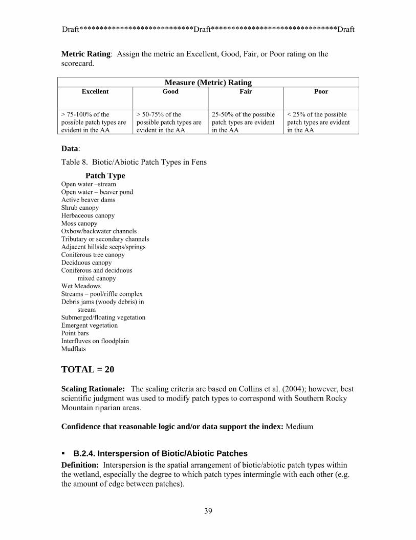
Draft****************************Draft*******************************Draft
Metric Rating: Assign the metric an Excellent, Good, Fair, or Poor rating on the scorecard.
Measure (Metric) Rating Excellent Good Fair Poor
> 75-100% of the possible patch types are evident in the AA
> 50-75% of the possible patch types are evident in the AA
25-50% of the possible patch types are evident in the AA
< 25% of the possible patch types are evident in the AA
Data:
Table 8. Biotic/Abiotic Patch Types in Fens
Patch Type Open water –stream Open water – beaver pond Active beaver dams Shrub canopy Herbaceous canopy Moss canopy Oxbow/backwater channels Tributary or secondary channels Adjacent hillside seeps/springs Coniferous tree canopy Deciduous canopy Coniferous and deciduous
mixed canopy Wet Meadows Streams – pool/riffle complex Debris jams (woody debris) in
stream Submerged/floating vegetation Emergent vegetation Point bars Interfluves on floodplain Mudflats TOTAL = 20 Scaling Rationale: The scaling criteria are based on Collins et al. (2004); however, best scientific judgment was used to modify patch types to correspond with Southern Rocky Mountain riparian areas. Confidence that reasonable logic and/or data support the index: Medium
B.2.4. Interspersion of Biotic/Abiotic Patches Definition: Interspersion is the spatial arrangement of biotic/abiotic patch types within the wetland, especially the degree to which patch types intermingle with each other (e.g. the amount of edge between patches).
39

Draft****************************Draft*******************************Draft
Background: This metric is one aspect of the condition of specific occurrences of wetland and riparian ecological systems. Rationale for Selection of the Variable: Spatial complexity of biotic/abiotic patches is indicative of intact ecological processes (Collins et al. 2004). Unimpacted sites have an expected spatial pattern of biotic/abiotic patches. Human-induced alterations can decrease this complexity and homogenize patch distribution. Measurement Protocol: This metric is measured by determining the degree of interspersion of biotic/abiotic patches present in the riparian area. This can be completed in the field for most riparian areas, however aerial photography may be beneficial for larger sites (Collin et al. 2004). The metric is rated by matching site interspersion with the categorical ratings in the scorecard. Metric Rating: Assign the metric an Excellent, Good, Fair, or Poor rating on the scorecard.
Measure (Metric) Rating Excellent Good Fair Poor
Horizontal structure consists of a very complex array of nested and/or interspersed, irregular biotic/abiotic patches, with no single dominant patch type
Horizontal structure consists of a moderately complex array of nested or interspersed biotic/abiotic patches, with no single dominant patch type
Horizontal structure consists of a simple array of nested or interspersed biotic/abiotic patches,
Horizontal structure consists of one dominant patch type and thus has relatively no interspersion
Data: See B.2.3 for list and definitions of Biotic Patches. Scaling Rationale: The scaling criteria are based on Collin et al. (2004), however best scientific judgment was used to modify criteria to correspond with Southern Rocky Mountain riparian areas. Confidence that reasonable logic and/or data support the index: Medium
B.2.5. Saplings/seedlings of Native Woody Species Definition: This metric estimates the amount of regeneration of native woody plants. Background: This metric is one aspect of the condition of specific occurrences of wetland and riparian ecological systems. Rationale for Selection of the Variable: Intensive grazing by domestic livestock and/or alteration of natural flow regime can reduce to eliminate regeneration by native woody plants (Elmore and Kauffman 1994). Species such as willows depend on episodic
40

Draft****************************Draft*******************************Draft
flooding to create new bare surfaces suitable for germination of willow seedlings (Woods 2001). In addition, base flows following flooding need to be high enough to maintain soil water content in these areas at or above 15% through July and August in order for these seedlings to survive long enough to establish a deep root system (Woods 2001). Beaver dams also create bare areas suitable for regeneration of woody species, especially as they accumulate silt and/or there is a breach in the dam. Lack of regeneration is indicative of altered ecological processes and has adverse impacts to the biotic integrity of the riparian area. Measurement Protocol: This metric is measured by determining the degree of regeneration of native woody species present along the streambank and edges of beaver ponds/dams. This is completed in the field and ocular estimates are used to match regeneration with the categorical ratings in the scorecard. Metric Rating: Assign the metric an Excellent, Good, Fair, or Poor rating on the scorecard.
Measure (Metric) Rating Excellent Good Fair Poor
Saplings/seedlings of native woody species (cottonwood/willow) present in expected amount; Obvious regeneration.
Saplings/seedlings of native woody species (cottonwood/willow) present but less than expected; Some seedling/saplings present.
Saplings/seedlings of native woody species (cottonwood/willow) present but in low abundance; Little regeneration by native species.
No reproduciton of native woody species
Data: N/A Scaling Rationale: The criteria are based on best scientific judgment. Confidence that reasonable logic and/or data support the index: Medium
B.3 Abiotic Condition Metrics
B.3.1 Land Use Within the Wetland Definition: This metric addresses the intensity of human dominated land uses within the riparian area. Background: This metric is one aspect of the condition of specific occurrences of wetland and riparian ecological systems. Rationale for Selection of the Variable: The intensity of human activity in the riparian area often has a proportionate impact on the ecological processes occurring onsite. Each
41

Draft****************************Draft*******************************Draft
land use type is assigned a coefficient ranging from 0.0 to 1.0 indicating its relative impact to the riparian area (Hauer et al. 2002). Measurement Protocol: This metric is measured by documenting land use(s) within the riparian area. This should be completed in the field then verified in the office using aerial photographs or GIS. However, with access to current aerial photography and/or GIS data a rough calculation of Land Use can be made in the office. Ideally, both field data as well as remote sensing tools are used to identify an accurate % of each land use within 100 m of the riparian area edge. To calculate a Total Land Use Score estimate the % of the riparian area under each Land Use type and then plug the corresponding coefficient (Table 5) with some manipulation to account for regional application) into the following equation:
Sub-land use score = ∑ LU x PC⁄100
where: LU = Land Use Score for Land Use Type; PC = % of adjacent area in Land Use Type.
Do this for each land use, then sum the Sub-Land Use Score(s) to arrive at a Total Land Score. For example, if 30% of the riparian area was under moderate grazing (0.3 * 0.6 = 0.18), 10% composed of unpaved roads (0.1 * 0.1 = 0.01), and 40% was a natural area (e.g. no human land use) (1.0 * 0.4 = 0.4), the Total Land Use Score would = 0.59 (0.18 + 0.01 + 0.40). Metric Rating: Assign the metric an Excellent, Good, Fair, or Poor rating on the scorecard.
Measure (Metric) Rating Excellent Good Fair Poor
Average Land Use Score = 1.0-0.95
Average Land Use Score = 0.80-0.95
Average Land Use Score = 0.4-0.80
Average Land Use Score = < 0.4
Data:
Table 9. Current Land Use and Corresponding Land Use Coefficients (based on Table 21 in Hauer ete al. (2002))
Current Land Use Coefficient Paved roads/parking lots/domestic or commercially developed buildings/gravel pit operation 0.0 Unpaved Roads (e.g., driveway, tractor trail) / Mining 0.1 Agriculture (tilled crop production) 0.2 Heavy grazing by livestock / intense recreation (ATV use/camping/popular fishing spot, etc.) 0.3 Logging or tree removal with 50-75% of trees >50 cm dbh removed 0.4 Hayed 0.5 Moderate grazing 0.6 Moderate recreation (high-use trail) 0.7 Selective logging or tree removal with <50% of trees >50 cm dbh removed 0.8 Light grazing / light recreation (low-use trail) 0.9
42
Draft****************************Draft*******************************Draft
Fallow with no history of grazing or other human use in past 10 yrs 0.95 Natural area / land managed for native vegetation 1.0 Scaling Rationale: The coefficients were assigned according to best scientific judgment regarding each land use’s potential impact (Hauer et al. 2002). Land uses have differing degrees of potential impact. Some land uses have minimal impact, such as simply altering the integrity of native vegetation (e.g., recreation and grazing), while other activities (e.g., hay production and agriculture) may replace native vegetation with nonnative or cultural vegetation yet still provide potential cover for species movement. Intensive land uses (i.e., urban development, roads, mining, etc.) may completely destroy vegetation and drastically alter hydrological processes. Confidence that reasonable logic and/or data support the index: Medium.
B.3.2. Sediment Loading Index Definition: The sediment loading index is a measure of the varying degrees to which different land uses contribute excess sediment via surface water runoff and overland flow into a riparian area. Background: This metric is one aspect of the condition of specific occurrences of wetland and riparian ecological systems. Rationale for Selection of the Variable: The type and amount of each land use in the riparian area and contributing watershed affects the amount of sediment that enters into a riparian area. Excess sediment can change nutrient cycling, bury vegetation, suppress regeneration of plants, and carry pollutants into the riparian area. In a functional assessment of slope and depressional wetlands associated with the Great Salt Lake, Keate (2005) developed a HGM assessment model primarily based on land use as a surrogate for human impacts on wetland functions. Coefficients from Nnadi (1997) were used to represent the sediment, nutrient loading, runoff, and wildlife impacts associated with various land uses. The functions considered included hydrologic, geochemical and habitat characteristics. The same coefficients used in the Keate (2005) method are used for this metric. Measurement Protocol: Identify and estimate the percentage of each land use within the riparian area and the contributing watershed (within 100 m of the riparian area). This is best completed in the field, however with access to current aerial photography a rough calculation of Land Use can be made in the office. Ideally, both field data as well as remote sensing tools are used to identify an accurate % of each land use. Once the percentage of each land use is identified, multiply it by the corresponding Sediment Loading coefficient found for each land use in Appendix B, then sum for the Sediment Loading Index Score. For example, if 50% of the riparian area and contributing watershed (within 100 m of the riparian area) was multi-family residential, 20% had a dirt/local roads, and 30% natural
43

Draft****************************Draft*******************************Draft
vegetation the calculation would be (0.5 * 0.61) + (0.2 * 0.97) + (0.3* 1.0) = 0.79 (Sediment Loading Index Score). Referring to the scorecard, this would give the metric a “Fair” rating. The contributing watershed can be calculated or digitized using Digital Elevation Models in a GIS. Surface water divides are determined using topography and although groundwater divides do not always coincide with these same hydrological divides, groundwater movement is assumed to do so, unless other data for the site is available. Metric Rating: Assign the metric an Excellent, Good, Fair, or Poor rating on the scorecard.
Measure (Metric) Rating Excellent Good Fair Poor
Average Score = 0.9 – 1.0
Average Score = 0.8 – 0.89
Average Score = 0.75 – 0.79
Average Score = < 0.7
Data: Appendix B. Scaling Rationale: The scaling is based on best scientific judgment. Scores below 0.7 are assumed to have crossed a threshold in which loading impacts are considered to not be restoreable (based on the land uses that have coefficients below 0.7). Additional research may suggest changes to the scaling criteria. Confidence that reasonable logic and/or data support the index: Low/medium.
B.3.3. Upstream Surface Water Retention Definition: This metric measures the percentage of the contributing watershed which drains into water storage facilities (e.g., reservoirs, sediment basins, retention ponds, etc.) that are capable of storing surface water from several days to months (Smith 2000). Background: This metric is one aspect of the condition of specific occurrences of wetland and riparian ecological systems. Rationale for Selection of the Variable: Ecological processes of riparian areas are driven to a large degree by the magnitude and frequency of peak flows and the duration and volume of base flows (Poff et al. 1997). The biotic and physical integrity of riparian areas are dependent on the natural variation associated with these flow characteristics (Gregory et al. 1991; Poff et al. 1997). The amount of water retained in upstream facilities has a direct effect on these flows and subsequent effects on the continued biotic and physical integrity of the riparian area (Poff et al. 1997). For example, retention of surface water can decrease or eliminate episodic, high intensity flooding, decrease seasonal high flows (e.g., spring snowmelt) and increase base flows during seasonal dry periods causing a shift in channel morphology and altering the dispersal capabilities,
44
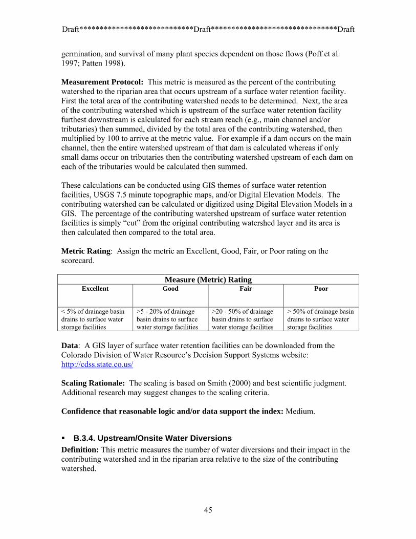
Draft****************************Draft*******************************Draft
germination, and survival of many plant species dependent on those flows (Poff et al. 1997; Patten 1998). Measurement Protocol: This metric is measured as the percent of the contributing watershed to the riparian area that occurs upstream of a surface water retention facility. First the total area of the contributing watershed needs to be determined. Next, the area of the contributing watershed which is upstream of the surface water retention facility furthest downstream is calculated for each stream reach (e.g., main channel and/or tributaries) then summed, divided by the total area of the contributing watershed, then multiplied by 100 to arrive at the metric value. For example if a dam occurs on the main channel, then the entire watershed upstream of that dam is calculated whereas if only small dams occur on tributaries then the contributing watershed upstream of each dam on each of the tributaries would be calculated then summed. These calculations can be conducted using GIS themes of surface water retention facilities, USGS 7.5 minute topographic maps, and/or Digital Elevation Models. The contributing watershed can be calculated or digitized using Digital Elevation Models in a GIS. The percentage of the contributing watershed upstream of surface water retention facilities is simply “cut” from the original contributing watershed layer and its area is then calculated then compared to the total area. Metric Rating: Assign the metric an Excellent, Good, Fair, or Poor rating on the scorecard.
Measure (Metric) Rating Excellent Good Fair Poor
< 5% of drainage basin drains to surface water storage facilities
>5 - 20% of drainage basin drains to surface water storage facilities
>20 - 50% of drainage basin drains to surface water storage facilities
> 50% of drainage basin drains to surface water storage facilities
Data: A GIS layer of surface water retention facilities can be downloaded from the Colorado Division of Water Resource’s Decision Support Systems website: http://cdss.state.co.us/ Scaling Rationale: The scaling is based on Smith (2000) and best scientific judgment. Additional research may suggest changes to the scaling criteria. Confidence that reasonable logic and/or data support the index: Medium.
B.3.4. Upstream/Onsite Water Diversions Definition: This metric measures the number of water diversions and their impact in the contributing watershed and in the riparian area relative to the size of the contributing watershed.
45

Draft****************************Draft*******************************Draft
Background: This metric is one aspect of the condition of specific occurrences of wetland and riparian ecological systems. Rationale for Selection of the Variable: Ecological processes of riparian areas are driven to a large degree by the magnitude and frequency of peak flows and the duration and volume of base flows (Poff et al. 1997). The biotic and physical integrity of riparian areas are dependent on the natural variation associated with these flow characteristics (Gregory et al. 1991; Poff et al. 1997). The amount of water imported, exported, or diverted from a watershed can affect these processes by decreasing episodic, high intensity flooding, seasonal high flows (e.g., spring snowmelt), and base flows (Poff et al. 1997; Patten 1998). Measurement Protocol: This metric can be measured by calculating the total number of water diversions occurring in the upstream contributing watershed as well as those onsite. The number of diversions relative to the size of the contributing basin is considered and then compared to the scorecard to determine the rating. Since the riparian area may occur on a variety of stream orders and since the corresponding upstream or contributing watershed differs in area, it is difficult to set standard guidelines. Thus, the user must use their best scientific judgment regarding the number of diversions and their impact relative to the size of the contributing watershed. If available, attributes such as capacity (cubic feet/second) of each diversion can be considered in the assessment. Metric Rating: Assign the metric an Excellent, Good, Fair, or Poor rating on the scorecard.
Measure (Metric) Rating Excellent Good Fair Poor
No upstream or onsite water diversions present
Few diversions present or impacts from diversions minor relative to contributing watershed size. Onsite diversions, if present, appear to have only minor impact on local hydrology.
Many diversions present or impacts from diversions moderate relative to contributing watershed size. Onsite diversions, if present, appear to have a major impact on local hydrology.
Water diversions are very numerous or impacts from diversions high relative to contributing watershed size. Onsite diversions, if present, have drastically altered local hydrology.
Data: A GIS layer of surface water diversions can be downloaded from the Colorado Division of Water Resource’s Decision Support Systems website: http://cdss.state.co.us/ Scaling Rationale: The scaling is based on best scientific judgment. Additional research is needed and may suggest changes to the scaling criteria. Confidence that reasonable logic and/or data support the index: Low/Medium.
46

Draft****************************Draft*******************************Draft
B.3.5. Floodplain Interaction Definition: This metric indicates the amount of interaction between the stream and floodplain by assessing whether any geomorphic modifications have been made to the stream channel. Background: This metric is one aspect of the condition of specific occurrences of wetland and riparian ecological systems. Rationale for Selection of the Variable: Overbank flooding is a critical ecological process in riparian areas as it replenishes floodplain aquifers, deposits and/or removes sediment, detritus, and nutrients in the floodplain. Stream channels affected by geomorphic modifications (e.g., channel incision, dikes, levees, roads, bridges, rip-rap, etc.) lose their connection to the adjacent floodplain and the ability to migrate (Poff et al. 1997). The biotic and physical integrity of riparian areas are partially dependent on the natural variation associated with overbank flows (Gregory et al. 1991; Poff et al. 1997). Measurement Protocol: This metric is estimated in the field by observing signs of overbank flooding, channel migration, and geomorphic modifications that are present within the riparian area. From these observations, best scientific judgment is used to assign the metric rating in the scorecard. Metric Rating: Assign the metric an Excellent, Good, Fair, or Poor rating on the scorecard.
Measure (Metric) Rating Excellent Good Fair Poor
Floodplain interaction is within natural range of variability. There are no geomorphic modifications (incised channel, dikes, levees, riprap, bridges, road beds, etc.) made to contemporary floodplain.
Floodplain interaction is disrupted due to the presence of a few geomorphic modifications. Up to 20% of streambanks are affected.
Floodplain interaction is highly disrupted due to multiple geomorphic modifications. Between 20 – 50% of streambanks are affected.
Complete geomorphic modification along river channel. The channel occurs in a steep, incised gulley due to anthropogenic impacts. More than 50% of streambanks are affected.
Data: N/A Scaling Rationale: The scaling is based on best scientific judgment. Additional research is needed and may suggest changes to the scaling criteria. Confidence that reasonable logic and/or data support the index: Low/Medium.
47

Draft****************************Draft*******************************Draft
B.3.6. Surface Water Runoff Index Definition: The surface water runoff index is a measure of the varying degrees to which different land uses alters surface water runoff and overland flow into a riparian area. Background: This metric is one aspect of the condition of specific occurrences of wetland and riparian ecological systems. Rationale for Selection of the Variable: The type and amount of each land use in the riparian area and contributing watershed affects the timing, duration, and frequency of surface water runoff and overland flow into a riparian area. These flows alter the hydrological regime of the riparian area and can result in degradation of biotic integrity, change nutrient cycling, and potentially affect physical integrity. In a functional assessment of slope and depressional wetlands associated with the Great Salt Lake, Keate (2005) developed a HGM assessment model primarily based on land use as a surrogate for human impacts on wetland functions. Coefficients from Nnadi (1997) were used to represent the sediment, nutrient loading, runoff, and wildlife impacts associated with various land uses. The functions considered included hydrologic, geochemical and habitat characteristics. The same coefficients used in the Keate (2005) method are used for this metric. Measurement Protocol: Identify and estimate the percentage of each land use within the riparian area and the contributing watershed (within 100 m of the riparian area). This is best completed in the field, however with access to current aerial photography a rough calculation of Land Use can be made in the office. Ideally, both field data as well as remote sensing tools are used to identify an accurate % of each land use. Once the percentage of each land use is identified, multiply it by the corresponding Surface Water Runoff coefficient found for each land use in Appendix B, then sum for the Surface Water Index Score. For example, if 50% of the riparian area and contributing watershed (within 100 m of the riparian area) was under heaving grazing, 10% had a dirt road, and 40% natural vegetation the calculation would be (0.5 * 0.76) + (0.1 * 0.71) + (0.4* 1.0) = 0.85 (Surface Water Index Score). Referring to the scorecard, this would give the metric a “Fair” rating. The contributing watershed can be calculated or digitized using Digital Elevation Models in a GIS. Surface water divides are determined using topography and although groundwater divides do not always coincide with these same hydrological divides, groundwater movement is assumed to do so, unless other data for the site is available
48

Draft****************************Draft*******************************Draft
Metric Rating: Assign the metric an Excellent, Good, Fair, or Poor rating on the scorecard.
Measure (Metric) Rating Excellent Good Fair Poor
Average Score = 0.9 – 1.0
Average Score = 0.8 – 0.89
Average Score = 0.75 – 0.79
Average Score = < 0.7
Data: Appendix B. Scaling Rationale: The scaling is based on best scientific judgment. Scores below 0.7 are assumed to have crossed a threshold in which runoff impacts are considered to not be restoreable (based on the land uses that have coefficients below 0.7). Additional research may suggest changes to the scaling criteria.
Confidence that reasonable logic and/or data support the index: Medium.
B.3.7. Index of Hydrological Alteration Definition: This metric uses daily streamflow data to determine trends at one site or determine differences between pre- and post-impacts of sites. Background: This metric is one aspect of the condition of specific occurrences of wetland and riparian ecological systems. Rationale for Selection of the Variable: The Index of Hydrological Alteration (IHA) is an easy to use tool for calculating the characteristics of natural and altered hydrologic regimes using any type of daily hydrologic data, such as streamflows, river stages, ground water levels, etc. Rather that review the entire method here, please refer to http://www.freshwaters.org/tools to download the IHA software as well as supporting documentation, including numerous published papers. Measurement Protocol: Long-term daily streamflow data are required for this metric. If those are not available daily flow data may be generated using a hydrologic model or other simulation method (see Richter et al. 1997). The IHA statistics will be meaningful only when calculated for a sufficiently long hydrologic record. The length of record necessary to obtain reliable comparisons is currently being researched, however it is recommended that at least twenty years of daily records be used (see Richter et al. 1997). Some lake level and ground water well data are also available from the USGS, but much of this type of data is collected and managed by other local governmental entities.
49
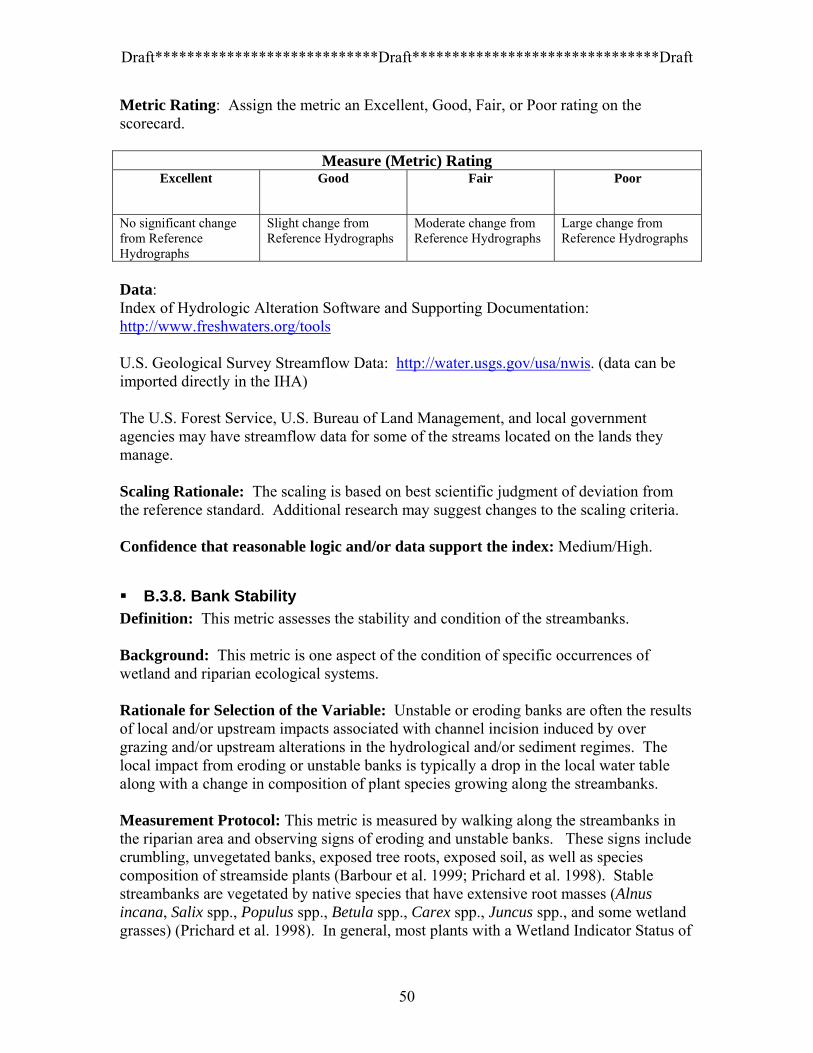
Draft****************************Draft*******************************Draft
Metric Rating: Assign the metric an Excellent, Good, Fair, or Poor rating on the scorecard.
Measure (Metric) Rating Excellent Good Fair Poor
No significant change from Reference Hydrographs
Slight change from Reference Hydrographs
Moderate change from Reference Hydrographs
Large change from Reference Hydrographs
Data: Index of Hydrologic Alteration Software and Supporting Documentation: http://www.freshwaters.org/tools U.S. Geological Survey Streamflow Data: http://water.usgs.gov/usa/nwis. (data can be imported directly in the IHA) The U.S. Forest Service, U.S. Bureau of Land Management, and local government agencies may have streamflow data for some of the streams located on the lands they manage. Scaling Rationale: The scaling is based on best scientific judgment of deviation from the reference standard. Additional research may suggest changes to the scaling criteria.
Confidence that reasonable logic and/or data support the index: Medium/High.
B.3.8. Bank Stability Definition: This metric assesses the stability and condition of the streambanks. Background: This metric is one aspect of the condition of specific occurrences of wetland and riparian ecological systems. Rationale for Selection of the Variable: Unstable or eroding banks are often the results of local and/or upstream impacts associated with channel incision induced by over grazing and/or upstream alterations in the hydrological and/or sediment regimes. The local impact from eroding or unstable banks is typically a drop in the local water table along with a change in composition of plant species growing along the streambanks. Measurement Protocol: This metric is measured by walking along the streambanks in the riparian area and observing signs of eroding and unstable banks. These signs include crumbling, unvegetated banks, exposed tree roots, exposed soil, as well as species composition of streamside plants (Barbour et al. 1999; Prichard et al. 1998). Stable streambanks are vegetated by native species that have extensive root masses (Alnus incana, Salix spp., Populus spp., Betula spp., Carex spp., Juncus spp., and some wetland grasses) (Prichard et al. 1998). In general, most plants with a Wetland Indicator Status of
50
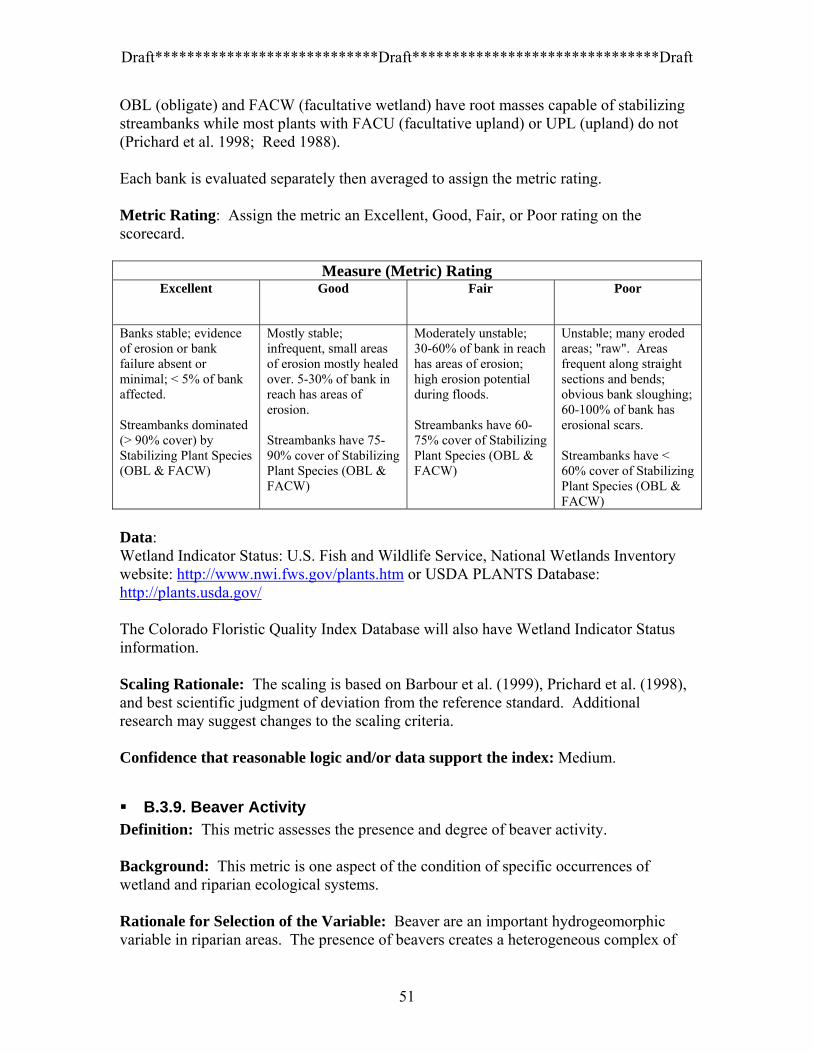
Draft****************************Draft*******************************Draft
OBL (obligate) and FACW (facultative wetland) have root masses capable of stabilizing streambanks while most plants with FACU (facultative upland) or UPL (upland) do not (Prichard et al. 1998; Reed 1988). Each bank is evaluated separately then averaged to assign the metric rating. Metric Rating: Assign the metric an Excellent, Good, Fair, or Poor rating on the scorecard.
Measure (Metric) Rating Excellent Good Fair Poor
Banks stable; evidence of erosion or bank failure absent or minimal; < 5% of bank affected. Streambanks dominated (> 90% cover) by Stabilizing Plant Species (OBL & FACW)
Mostly stable; infrequent, small areas of erosion mostly healed over. 5-30% of bank in reach has areas of erosion. Streambanks have 75-90% cover of Stabilizing Plant Species (OBL & FACW)
Moderately unstable; 30-60% of bank in reach has areas of erosion; high erosion potential during floods. Streambanks have 60-75% cover of Stabilizing Plant Species (OBL & FACW)
Unstable; many eroded areas; "raw". Areas frequent along straight sections and bends; obvious bank sloughing; 60-100% of bank has erosional scars. Streambanks have < 60% cover of Stabilizing Plant Species (OBL & FACW)
Data: Wetland Indicator Status: U.S. Fish and Wildlife Service, National Wetlands Inventory website: http://www.nwi.fws.gov/plants.htm or USDA PLANTS Database: http://plants.usda.gov/ The Colorado Floristic Quality Index Database will also have Wetland Indicator Status information. Scaling Rationale: The scaling is based on Barbour et al. (1999), Prichard et al. (1998), and best scientific judgment of deviation from the reference standard. Additional research may suggest changes to the scaling criteria.
Confidence that reasonable logic and/or data support the index: Medium.
B.3.9. Beaver Activity Definition: This metric assesses the presence and degree of beaver activity. Background: This metric is one aspect of the condition of specific occurrences of wetland and riparian ecological systems. Rationale for Selection of the Variable: Beaver are an important hydrogeomorphic variable in riparian areas. The presence of beavers creates a heterogeneous complex of
51
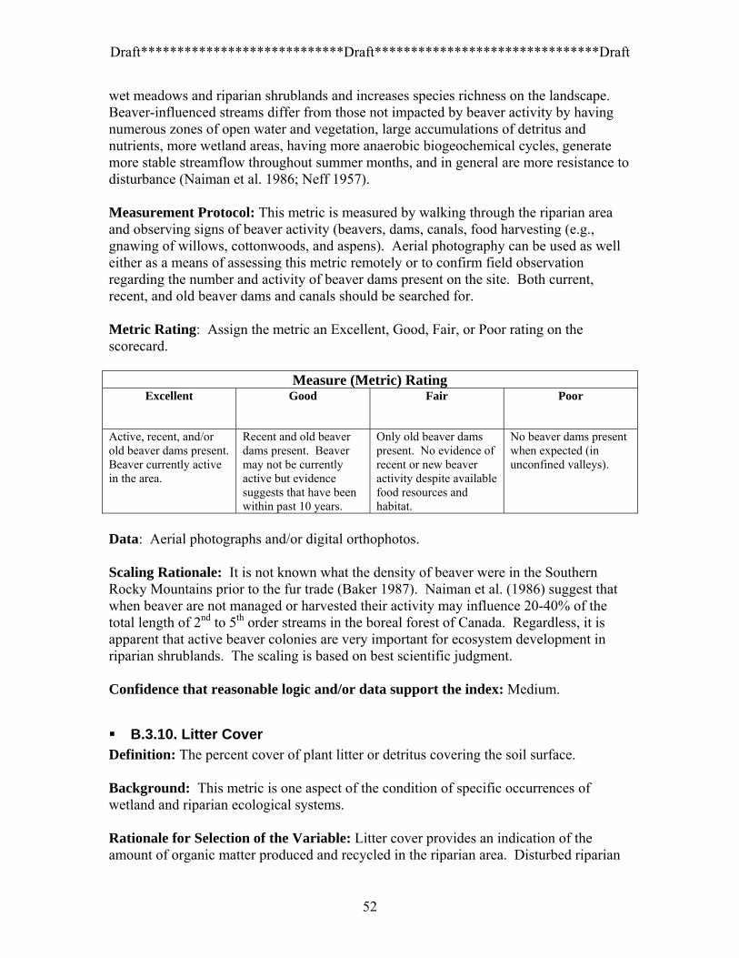
Draft****************************Draft*******************************Draft
wet meadows and riparian shrublands and increases species richness on the landscape. Beaver-influenced streams differ from those not impacted by beaver activity by having numerous zones of open water and vegetation, large accumulations of detritus and nutrients, more wetland areas, having more anaerobic biogeochemical cycles, generate more stable streamflow throughout summer months, and in general are more resistance to disturbance (Naiman et al. 1986; Neff 1957). Measurement Protocol: This metric is measured by walking through the riparian area and observing signs of beaver activity (beavers, dams, canals, food harvesting (e.g., gnawing of willows, cottonwoods, and aspens). Aerial photography can be used as well either as a means of assessing this metric remotely or to confirm field observation regarding the number and activity of beaver dams present on the site. Both current, recent, and old beaver dams and canals should be searched for. Metric Rating: Assign the metric an Excellent, Good, Fair, or Poor rating on the scorecard.
Measure (Metric) Rating Excellent Good Fair Poor
Active, recent, and/or old beaver dams present. Beaver currently active in the area.
Recent and old beaver dams present. Beaver may not be currently active but evidence suggests that have been within past 10 years.
Only old beaver dams present. No evidence of recent or new beaver activity despite available food resources and habitat.
No beaver dams present when expected (in unconfined valleys).
Data: Aerial photographs and/or digital orthophotos. Scaling Rationale: It is not known what the density of beaver were in the Southern Rocky Mountains prior to the fur trade (Baker 1987). Naiman et al. (1986) suggest that when beaver are not managed or harvested their activity may influence 20-40% of the total length of 2nd to 5th order streams in the boreal forest of Canada. Regardless, it is apparent that active beaver colonies are very important for ecosystem development in riparian shrublands. The scaling is based on best scientific judgment.
Confidence that reasonable logic and/or data support the index: Medium.
B.3.10. Litter Cover Definition: The percent cover of plant litter or detritus covering the soil surface. Background: This metric is one aspect of the condition of specific occurrences of wetland and riparian ecological systems. Rationale for Selection of the Variable: Litter cover provides an indication of the amount of organic matter produced and recycled in the riparian area. Disturbed riparian
52

Draft****************************Draft*******************************Draft
areas often have different amounts of litter cover than reference sites due to a change in species composition, productivity, and decomposition. Measurement Protocol: Litter cover is measured using the same protocols as vegetation. A qualitative, ocular estimate of litter cover is used to calculate and score the metric. The entire occurrence of the riparian system should be walked and a qualitative ocular estimate of the total cover of litter in the wetland should be made. Alternatively, if time and resources allow a more quantitative determination of species presence and cover such methods (i.e. Peet et al. 1998) are encouraged to be used. The metric is scored by comparing current litter cover values to those of reference or baseline conditions. Metric Rating: Assign the metric an Excellent, Good, Fair, or Poor rating on the scorecard.
Measure (Metric) Rating Excellent Good Fair Poor
No significant change from Reference Amount
Slight change from Reference Amount
Moderate change from Reference Amount
Large change from Reference Amount
Data: The Colorado Vegetation Index of Biotic Integrity project will likely provide the necessary data to establish the range of litter cover found in undisturbed examples. Scaling Rationale: The criteria are based on best scientific judgment. Confidence that reasonable logic and/or data support the index: Low/medium.
B.3.11. Nutrient/Pollutant Loading Index Definition: The nutrient/pollutant loading index is a measure of the varying degrees to which different land uses contributed excess nutrients and pollutants via surface water runoff and overland flow into a riparian area. Background: This metric is one aspect of the condition of specific occurrences of wetland and riparian ecological systems. Rationale for Selection of the Variable: The type and amount of each land use in the riparian area and contributing watershed affects the amounts and types of nutrients and pollutants that enter into a riparian area. Excess nutrients can result in degradation of biotic integrity, change nutrient cycling, and potentially affect peat integrity. In a functional assessment of slope and depressional wetlands associated with the Great Salt Lake, Keate (2005) developed a HGM assessment model primarily based on land use as a surrogate for human impacts on wetland functions. Coefficients from Nnadi (1997) were used to represent the sediment, nutrient loading, runoff, and wildlife impacts associated with various land uses. The functions considered included hydrologic,
53
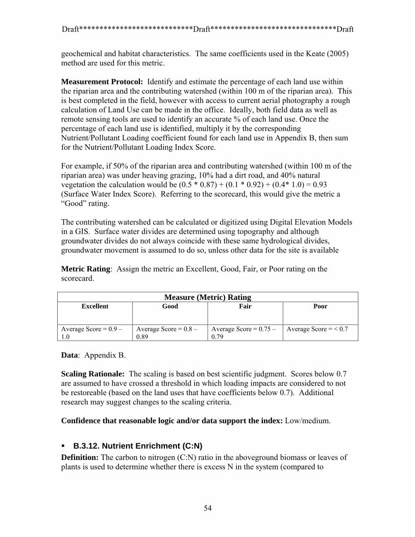
Draft****************************Draft*******************************Draft
geochemical and habitat characteristics. The same coefficients used in the Keate (2005) method are used for this metric. Measurement Protocol: Identify and estimate the percentage of each land use within the riparian area and the contributing watershed (within 100 m of the riparian area). This is best completed in the field, however with access to current aerial photography a rough calculation of Land Use can be made in the office. Ideally, both field data as well as remote sensing tools are used to identify an accurate % of each land use. Once the percentage of each land use is identified, multiply it by the corresponding Nutrient/Pollutant Loading coefficient found for each land use in Appendix B, then sum for the Nutrient/Pollutant Loading Index Score. For example, if 50% of the riparian area and contributing watershed (within 100 m of the riparian area) was under heaving grazing, 10% had a dirt road, and 40% natural vegetation the calculation would be (0.5 * 0.87) + (0.1 * 0.92) + (0.4* 1.0) = 0.93 (Surface Water Index Score). Referring to the scorecard, this would give the metric a “Good” rating. The contributing watershed can be calculated or digitized using Digital Elevation Models in a GIS. Surface water divides are determined using topography and although groundwater divides do not always coincide with these same hydrological divides, groundwater movement is assumed to do so, unless other data for the site is available Metric Rating: Assign the metric an Excellent, Good, Fair, or Poor rating on the scorecard.
Measure (Metric) Rating Excellent Good Fair Poor
Average Score = 0.9 – 1.0
Average Score = 0.8 – 0.89
Average Score = 0.75 – 0.79
Average Score = < 0.7
Data: Appendix B. Scaling Rationale: The scaling is based on best scientific judgment. Scores below 0.7 are assumed to have crossed a threshold in which loading impacts are considered to not be restoreable (based on the land uses that have coefficients below 0.7). Additional research may suggest changes to the scaling criteria. Confidence that reasonable logic and/or data support the index: Low/medium.
B.3.12. Nutrient Enrichment (C:N) Definition: The carbon to nitrogen (C:N) ratio in the aboveground biomass or leaves of plants is used to determine whether there is excess N in the system (compared to
54
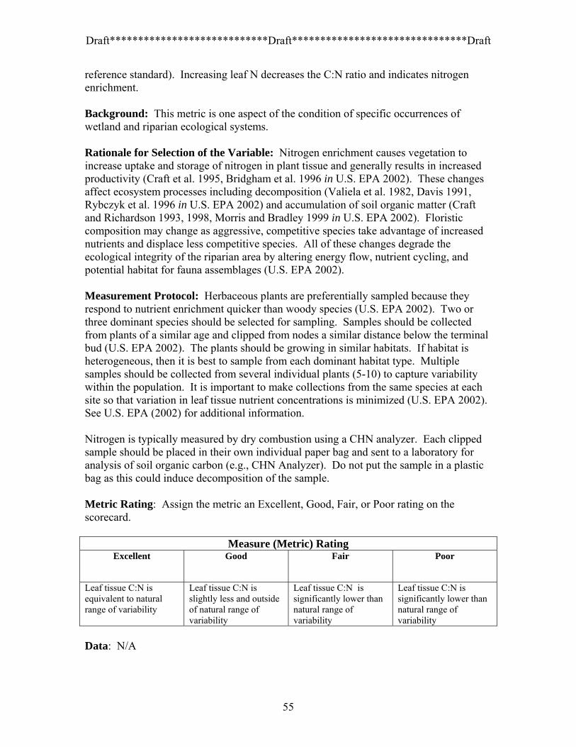
Draft****************************Draft*******************************Draft
reference standard). Increasing leaf N decreases the C:N ratio and indicates nitrogen enrichment. Background: This metric is one aspect of the condition of specific occurrences of wetland and riparian ecological systems. Rationale for Selection of the Variable: Nitrogen enrichment causes vegetation to increase uptake and storage of nitrogen in plant tissue and generally results in increased productivity (Craft et al. 1995, Bridgham et al. 1996 in U.S. EPA 2002). These changes affect ecosystem processes including decomposition (Valiela et al. 1982, Davis 1991, Rybczyk et al. 1996 in U.S. EPA 2002) and accumulation of soil organic matter (Craft and Richardson 1993, 1998, Morris and Bradley 1999 in U.S. EPA 2002). Floristic composition may change as aggressive, competitive species take advantage of increased nutrients and displace less competitive species. All of these changes degrade the ecological integrity of the riparian area by altering energy flow, nutrient cycling, and potential habitat for fauna assemblages (U.S. EPA 2002). Measurement Protocol: Herbaceous plants are preferentially sampled because they respond to nutrient enrichment quicker than woody species (U.S. EPA 2002). Two or three dominant species should be selected for sampling. Samples should be collected from plants of a similar age and clipped from nodes a similar distance below the terminal bud (U.S. EPA 2002). The plants should be growing in similar habitats. If habitat is heterogeneous, then it is best to sample from each dominant habitat type. Multiple samples should be collected from several individual plants (5-10) to capture variability within the population. It is important to make collections from the same species at each site so that variation in leaf tissue nutrient concentrations is minimized (U.S. EPA 2002). See U.S. EPA (2002) for additional information.
Nitrogen is typically measured by dry combustion using a CHN analyzer. Each clipped sample should be placed in their own individual paper bag and sent to a laboratory for analysis of soil organic carbon (e.g., CHN Analyzer). Do not put the sample in a plastic bag as this could induce decomposition of the sample. Metric Rating: Assign the metric an Excellent, Good, Fair, or Poor rating on the scorecard.
Measure (Metric) Rating Excellent Good Fair Poor
Leaf tissue C:N is equivalent to natural range of variability
Leaf tissue C:N is slightly less and outside of natural range of variability
Leaf tissue C:N is significantly lower than natural range of variability
Leaf tissue C:N is significantly lower than natural range of variability
Data: N/A
55
Draft****************************Draft*******************************Draft
Scaling Rationale: Reference C:N ratios need to be established in undisturbed riparian areas. Thereafter, the scaling is based on best scientific judgment and an assumed linear relationship of the amount of deviation from the reference standard to level of nutrient enrichment. If data are collected from riparian areas across a disturbance gradient, quantitative criteria could be established. Confidence that reasonable logic and/or data support the index: Medium/High.
B.3.13. Nutrient Enrichment (C:P) Definition: The carbon to phosphorous (C:P) ratio in the aboveground biomass or leaves of plants is used to determine whether there is excess P in the system (compared to reference standard). Increasing leaf P decreases the C:P ratio and indicates phosphorous enrichment. Background: This metric is one aspect of the condition of specific occurrences of wetland and riparian ecological systems. Rationale for Selection of the Variable: Phosphorous enrichment causes vegetation to increase uptake and storage of phosphorous in plant tissue and generally results in increased productivity (Craft et al. 1995, Bridgham et al. 1996 in U.S. EPA 2002). These changes affect ecosystem processes including decomposition (Valiela et al. 1982, Davis 1991, Rybczyk et al. 1996 in U.S. EPA 2002) and accumulation of soil organic matter (Craft and Richardson 1993, 1998, Morris and Bradley 1999 in U.S. EPA 2002). Floristic composition may change as aggressive, competitive species take advantage of increased nutrients and displace less competitive species. All of these changes degrade the ecological integrity of the riparian area by altering energy flow, nutrient cycling, and potential habitat for fauna assemblages (U.S. EPA 2002). Measurement Protocol: Herbaceous plants are preferentially sampled because they respond to nutrient enrichment quicker than woody species (U.S. EPA 2002). Two or three dominant species should be selected for sampling. Samples should be collected from plants of a similar age and clipped from nodes a similar distance below the terminal bud (U.S. EPA 2002). The plants should be growing in similar habitats. If habitat is heterogeneous, then it is best to sample from each dominant habitat type. Multiple samples should be collected from several individual plants (5-10) to capture variability within the population. It is important to make collections from the same species at each site so that variation in leaf tissue nutrient concentrations is minimized (U.S. EPA 2002). See U.S. EPA (2002) for additional information.
Phosphorous is typically measured by spectrophotometry in acid (H2SO4-H2O2) digests. Each clipped sample should be placed in their own individual paper bag and sent to a laboratory for analysis of soil organic carbon (e.g., CHN Analyzer). Do not put the sample in a plastic bag as this could induce decomposition of the sample.
56
Draft****************************Draft*******************************Draft
Metric Rating: Assign the metric an Excellent, Good, Fair, or Poor rating on the scorecard.
Measure (Metric) Rating Excellent Good Fair Poor
Leaf tissue C:P is equivalent to natural range of variability
Leaf tissue C:P is slightly less and outside of natural range of variability
Leaf tissue C:P is significantly lower than natural range of variability
Leaf tissue C:P is significantly lower than natural range of variability
Data: N/A Scaling Rationale: Reference C:P ratios need to be established in undisturbed riparian areas. Thereafter, the scaling is based on best scientific judgment and an assumed linear relationship of the amount of deviation from the reference standard to level of nutrient enrichment. If data are collected from riparian areas across a disturbance gradient, quantitative criteria could be established. Confidence that reasonable logic and/or data support the index: Medium/High.
B.3.14. Soil Organic Matter Decomposition Definition: This metric indicates the amount of decomposition of soil organic matter present in the soil and thus is an indicator measure of nutrient cycling. Background: This metric is one aspect of the condition of specific occurrences of wetland and riparian ecological systems. Rationale for Selection of the Variable: Soil organic matter generally refers to the organic fraction of the soil, including plant and animal residues at various stages of decomposition, as well as substances synthesized by the soil organisms (Neue 1984). Organic matter plays an extremely important role in the soil environment, including increasing water holding capacity, encouraging soil structure, has a high cation exchange capacity, and supplies essential nutrients (Brady 1990). Soil organic matter is accumulated in both the O and surface soil (either A or E) horizons in the soil profile. In some riparian areas, soils can be poorly developed, thus the A and E horizons are lumped into a “surface mineral soil horizon” (SMS-horizons) category for this metric (Hauer et al. 2002). The O horizon is found on the soil surface and is composed of various stages of decomposition. The SMS-horizons accumulate highly decomposed organic matter (e.g., humus), which often gives the horizon a dark, black color and high amount of colloids (Brady 1990). Deviation of the depth of the O horizon from reference conditions indicate under- or over-abundance or too fast or slow of a decomposition rate (Hauer et al. 2002). The depth and color of the SMS-horizons is used in this metric as an index of the ability of the
57

Draft****************************Draft*******************************Draft
soil to store nutrients and thus changes from reference conditions are assumed to be indicators of changes in the input of organic matter as well in nutrient cycling (Hauer et al. 2002). For example, human disturbance may cause lower productivity resulting in thinner and lighter colored SMS-horizons (Hauer et al. 2002). Alternatively, thicker SMS-horizons than the reference standard may result from increased sedimentation (Hauer et al. 2002). Measurement Protocol: The metric is calculated as an Organic Matter Decomposition Factor (OMDF) based on the depth of the O-horizon, the depth of the SMS-horizon, and the soil color value (from Munsell Soil Chart) of the SMS-horizon (Hauer et al. 2002). Multiple soil pits should be dug in the riparian area to a depth where the lower boundary of the SMS-horizon is detected. If quantitative vegetation data are being collected, soil pits should be located within these plots to allow correlations with vegetation data. For example, if using the 20 x 50 m plots described by Peet et al. (1998), soil pits would be located within each of the intensive modules. The thickness of the O and SMS-horizons should be measured and the soil color estimated using a Munsell Soil Color Chart.
The OMDF is calculated as: OMDF = ( ) ⎥⎦
⎤⎢⎣
⎡⎟⎠⎞
⎜⎝⎛+
alueSoilColorVrizonDepthSMShozonDepthOhori
Metric Rating: Assign the metric an Excellent, Good, Fair, or Poor rating on the scorecard.
Measure (Metric) Rating Excellent Good Fair Poor
Mature Cottonwood areas: OMDF > 2.25; Immature cottonwood areas & cottonwood/ willow seedlings: OMDF > 0.8
Mature Cottonwood areas: OMDF 1.1 - 2.25; Immature cottonwood areas & cottonwood/ willow seedlings: OMDF 0.4 - 0.8
Mature Cottonwood areas: OMDF 0.5 - 1.1; Immature cottonwood areas & cottonwood/ willow seedlings: OMDF 0.2 - 0.4
Mature Cottonwood areas: OMDF < 0.5; Immature cottonwood areas & cottonwood/ willow seedlings: OMDF < 0.2
Data: N/A Scaling Rationale: The reference OMDF values are based on the work of Hauer et al. (2002) who found that riparian shrublands (e.g., willows and alders) and wet meadows in riverine floodplains in the Northern Rockies had OMDF values > 1.8. This reference value is tentatively used for Southern Rocky Mountain riparian shrublands, but additional data collection may suggest alternative values. The scaling is based on best scientific judgment and an assumed linear relationship of the amount of deviation from the reference standard to level of disturbance. If data are collected from riparian areas across a disturbance gradient, quantitative criteria could be established. Alternatively if “baseline” OMDF levels are known (from “pre-impact”
58
Draft****************************Draft*******************************Draft
conditions or from adjacent unaltered sites) then this metric can be used to determine change of OMDF with time. Confidence that reasonable logic and/or data support the index: Medium.
B.3.15. Soil Organic Carbon Definition: This metric measures the amount of soil organic carbon present in the soil. Background: This metric is one aspect of the condition of specific occurrences of wetland and riparian ecological systems. Rationale for Selection of the Variable: Soil organic matter or carbon generally refers to the organic fraction of the soil, including plant and animal residues at various stages of decomposition, as well as substances synthesized by the soil organisms (Neue 1984). Organic matter plays an extremely important role in the soil environment, including increases water holding capacity, encouraging soil structure, has a high cation exchange capacity, and supplies essential nutrients (Brady 1990). Soil organic carbon is strong metric of soil quality due to its sensitivity to environmental disturbance (NRC 2000 in Fennessy et al. 2004). Given that soil organic carbon contributes to critical hydrologic, biogeochemical, and physical processes, a reduction in soil organic carbon from reference conditions serves as a strong indicator of loss of soil quality. Measurement Protocol: Multiple soil pits should be dug in the riparian area to a depth of at least 40 cm. If quantitative vegetation data are being collected, soil pits should be located within these plots to allow correlations with vegetation data. For example, if using the 20 x 50 m plots described by Peet et al. (1998), soil pits would be located within each of the intensive modules. At least five replicate soil samples should be taken within the top 10 cm of the soil surface in each pit. The replicates are mixed together as “one” sample from the site. Each soil sample should be placed in their own individual plastic bag, packed on ice, and sent to a laboratory for analysis of soil organic carbon (e.g., CHN Analyzer). Metric Rating: Assign the metric an Excellent, Good, Fair, or Poor rating on the scorecard.
Measure (Metric) Rating Excellent Good Fair Poor
Soil C is equivalent to natural range of variability
Soil C is nearly equivalent to natural range of variability
Soil C is significantly lower than natural range of variability
Soil C is significantly lower than natural range of variability
Data: N/A
59
Draft****************************Draft*******************************Draft
Scaling Rationale: Reference soil organic carbon levels need to be established in undisturbed riparian areas. Thereafter, the scaling is based on best scientific judgment and an assumed linear relationship of the amount of deviation from the reference standard to level of disturbance. If data are collected from riparian areas across a disturbance gradient, quantitative criteria could be established. Alternatively, if “baseline” soil organic carbon levels are known (from “pre-impact” conditions or from adjacent unaltered sites) then this metric can be used to determine change of soil organic carbon with time. Confidence that reasonable logic and/or data support the index: Medium/High.
B.3.16. Soil Bulk Density Definition: Soil bulk density is a ratio of the mass/volume of the soil. This metric is a measure of the compaction of the soil horizons. Background: This metric is one aspect of the condition of specific occurrences of wetland and riparian ecological systems. Rationale for Selection of the Variable: Bulk density is a measure of the weight of the soil divided by its volume and provides an indication of the level of compaction. Compaction can result from any activity which compresses soil particles thereby increasing the weight to volume ratio. This can reduce the soil’s water holding capacity, infiltration rate, water movement through the soil, and limit plant growth by physically restricting root growth (NRCS 2001). Bulk density of organic soils are typically much less than those of mineral soils, however as decomposition increases and/or organic soils are compacted from human activity, bulk density of organic soils will increase. This has corresponding negative impacts on ecological processes such as water movement through the peat body, decomposition, and nutrient cycling. Measurement Protocol: Multiple soil pits should be dug in the riparian area to a depth of at least 40 cm. If quantitative vegetation data are being collected, soil pits should be located within these plots to allow correlations with vegetation data. For example, if using the 20 x 50 m plots described by Peet et al. (1998), soil pits would be located and samples collected within each of the intensive modules. The samples are collected by taking a core sample within the top 15 cm of the soil. A cylinder of known volume should be used to collect samples. A PVC pipe of known dimensions will suffice. The cylinder is simply inserted into the soil profile, extracted, then shaved to eliminate any soil which is not contained within the cylinder. The soil remaining in the cylinder can then be placed into a plastic bag and then sent to a laboratory for analysis. Bulk density and soil texture (e.g., particle distribution) should be analyzed. Alternatively, texture can be determined in the field using the “field hand method”, however lab analysis is preferable.
60

Draft****************************Draft*******************************Draft
Once texture and bulk density are determined, use the information below to determine whether the soil’s bulk density is less than, equal to, or greater then the minimum root-restricting bulk density values listed for the corresponding texture of the soil and assign the metric rating accordingly in the scorecard. There are no root restricting values given for organic soils, thus if the riparian area is dominated by organic soil, reference bulk density measurements need to be established in undisturbed areas. Metric Rating: Assign the metric an Excellent, Good, Fair, or Poor rating on the scorecard.
Measure (Metric) Rating Excellent Good Fair Poor
Bulk density value for riparian area is at least 0.2 (g/cm3) less than Root Restricting Bulk Density value for the soil texture found in the riparian area.
Bulk density value for riparian area is at least 0.2 (g/cm3) less than Root Restricting Bulk Density value for the soil texture found in the riparian area. (same as Very Good)
Bulk density for riparian area is between 0.2 to 0.1 (g/cm3) less than Root Restricting Bulk Density value for the soil texture found in the riparian area.
Bulk density for riparian area is = or > than Root Restricting Bulk Density value for the soil texture found in the riparian area.
Data: The data below are derived from a Natural Resource Conservation Service, Soil Quality Information Sheet — Compaction which can be found online at: http://soils.usda.gov/sqi/publications/sqis.html Theses texture classes have the following Root Restricting Bulk Density values (g/cm3): 1. Coarse, medium, and fine sand AND loamy sand other than loamy very fine sand = 1.8 g/cm3 2. Very fine sand, loamy very find sand = 1.77 g/cm3 3. Sandy loam = 1.75 g/cm3 4. Loam, sandy clay loam = 1.7 g/cm3 5. Clay loam = 1.65 g/cm3 6. Sandy clay = 1.6 g/cm3 7. Silt, silt loam = 1.55 g/cm3 8. Silty clay loam = 1.5 g/cm3 9. Silty clay = 1.45 g/cm3 10. Clay = 1.4 g/cm3 Scaling Rationale: The scaling is based on best scientific judgment and an assumed linear relationship of the amount of deviation from the reference standard to level of disturbance. However, no distinction was made between Excellent and Good as there is no information to suggest that threshold. Alternatively if “baseline” bulk density levels are known (from “pre-impact” conditions or from adjacent unaltered areas) then this metric can be used to determine change of bulk density with time. Confidence that reasonable logic and/or data support the index: Medium/High.
61

Draft****************************Draft*******************************Draft
B.4 Size Metrics
B.4.1. Absolute Size Definition: Absolute size is the current size of the riparian area. Background: This metric is one aspect of the size of specific occurrences of wetland and riparian ecological systems. Rationale for Selection of the Variable: Absolute size is pertinent to ecological integrity if the surrounding landscape is impacted by human-induced disturbances. When the surrounding landscape is impacted and has the potential to affect the wetland, larger sized wetlands are able to buffer against these impacts better than smaller sized wetlands due to the fact they generally possess a higher diversity of abiotic and biotic processes allowing them to recover and remain more resilient. However, when the landscape is unimpacted (i.e. has an “Excellent” rating), then absolute size has little impact on ecological integrity since there are no adjacent impacts to buffer. Of course, larger riparian areas tend to have more diversity (MacArthur and Wilson 1967); however, this is a metric more pertinent to functional or conservation value than ecological integrity. Thus, absolute size is included as a metric but is only considered in the overall ecological integrity rank if the landscape is impacted. Regardless, absolute size provides important information to conservation planners and land managers. Measurement Protocol: Absolute size can be measured easily in GIS using aerial photographs, orthophoto quads, National Wetland Inventory maps, etc. Absolute size can also be estimated in the field using 7.5 minute topographic quads, National Wetland Inventory maps, or a global positioning system. Riparian area boundaries aren’t delineated using jurisdictional methods (U.S. Army Corps of Engineers 1987) rather by the guidelines identified for delineating the boundaries of the riparian ecological system type. Metric Rating: Assign the metric an Excellent, Good, Fair, or Poor rating on the scorecard.
Measure (Metric) Rating Excellent Good Fair Poor
> 8.0 linear km (minimum of 10 m wide)
5.0 to 8.0 linear km (minimum of 10 m wide)
1.5 to 5.0 linear km (minimum of 10 m wide)
< 1.5 linear km (minimum of 10 m wide)
Data: N/A
62

Draft****************************Draft*******************************Draft
Scaling Rationale: Scaling criteria are based on Rondeau (2001) and best scientific judgment. Confidence that reasonable logic and/or data support the index: Medium/High.
B.4.2. Relative Size Definition: Relative size is the current size of the riparian area divided by the total potential size of the riparian area multiplied by 100. Background: This metric is one aspect of the size of specific occurrences of wetland and riparian ecological systems. Rationale for Selection of the Variable: Relative size is an indication of the amount of the riparian area lost due to human-induced disturbances. It provides information allowing the user to calibrate the Absolute Size metric to the abiotic potential of the riparian area onsite. For example, if a riparian area has an Absolute Size of 2 hectares but the Relative Size is 50% (1 hectare), this indicates that half of the original riparian area has been lost or severely degraded. Unlike Absolute Size, the Relative Size metric is always considered in the ecological integrity rank. Measurement Protocol: Relative size can be measured in GIS using aerial photographs, orthophoto quads, National Wetland Inventory maps, etc. However, field calibration of size is required since it can be difficult to discern the abiotic potential of the riparian area from remote sensing data. However, the reverse may also be true since old or historic aerial photographs may indicate a larger riparian area than observed in the field. Relative size can also be estimated in the field using 7.5 minute topographic quads, National Wetland Inventory maps, or a global positioning system. Riparian area boundaries aren’t delineated using jurisdictional methods (U.S. Army Corps of Engineers 1987) rather by the guidelines identified for delineating the boundaries of the riparian ecological system type.
63

Draft****************************Draft*******************************Draft
Metric Rating: Assign the metric an Excellent, Good, Fair, or Poor rating on the scorecard.
Measure (Metric) Rating Excellent Good Fair Poor
Riparian area = onsite Abiotic Potential
Riparian area < Abiotic Potential; < 10% of riparian area has been reduced (destroyed or severely disturbed e.g change in hydrology) due to roads, impoundments, development, human-induced drainage, etc.
Riparian area < Abiotic Potential; 10-25% of riparian area has been reduced (destroyed or severely disturbed e.g change in hydrology) due to roads, impoundments, development, human-induced drainage, etc.
Riparian area < Abiotic Potential; > 25% of riparian area has been reduced (destroyed or severely disturbed e.g change in hydrology) due to roads, impoundments, development, human-induced drainage, etc.
Data: N/A Scaling Rationale: Scaling criteria are based on Rondeau (2001) and best scientific judgment. Confidence that reasonable logic and/or data support the index: Medium/High.
64
Draft****************************Draft*******************************Draft
C. REFERENCES Andreas, B.K. and R.W. Lichvar. 1995. Floristic index for establishing assessment standards: A case study for northern Ohio. Technical Report WRP-DE-8, U.S. Army Corps of Engineer Waterways Experiment Station, Vicksburg, MS. Baker, W.L. 1987. Recent Changes in the Riparian Vegetation of the Montane and Subalpine Zones of Western Colorado, U.S.A. PhD Dissertation. University of Wisconsin. Madison, WI. Baker, W.L. 1988. Size-class structure of contiguous riparian woodlands along a Rocky Mountain river. Physical Geography 9(1):1-14. Baker, W.L. 1989a. Macro- and Micro-scale Influences on Riparian Vegetation in Western Colorado. Annals of the Association of American Geographers 79(1): 65-78. Baker, W. L. 1989b. Classification of the riparian vegetation of the montane and subalpine zones in western Colorado. Great Basin Naturalist 49(2):214-228. Baker, W.L. 1990. Species richness of Colorado riparian vegetation. Journal of Vegetation Science 1: 119-124. Barbour, M.T., J. Gerritsen, B.D. Snyder, and J.B. Stribling. 1999. Rapid Bioassessment Protocols for Use in Streams and Wadeable Rivers: Periphyton, Benthic Macroinvertebrates and Fish, Second Edition. EPA 841-B-99-002. U.S. Environmental Protection Agency; Office of Water; Washington, D.C. Bierly, K.F. 1972. Meadow and Fen Vegetation in Big Meadows, Rocky Mountain National Park. M.S. Thesis. Colorado State University, Fort Collins, CO. Brady, N.C. 1990. The Nature and Properties of Soils. MacMillian Publishing, New York, NY. Bridgham SD, Pastor J, Jannsens JA, Chapin C, Malterer TJ. 1996. Multiple limiting gradients in peatlands: a call for a new paradigm. Wetlands 16:45-65. Castelle, A.J., C. Conolly, M. Emers, E.D. Metz, S. Meyer, M. Witter, S. Mauermann, T. Erickson, S.S. Cooke. 1992. Wetland Buffers: Use and Effectiveness. Adolfson Associates, Inc., Shorelands and Coastal Zone Management Program, Washington Department of Ecology, Olympia, Pub. No. 92-10. Coffee Creek Watershed Conservancy. 2001. 2001 Monitoring reports. http://www.coffeecreekwc.org/ccwc/ccwcmission/monitoring_reports.htmCoffee Creek Watershed Conservancy, Chesterton, IN.
65

Draft****************************Draft*******************************Draft
Collins, J.N., E. Stein, and M. Sutula. 2004. California Rapid Assessment Method for Wetlands V.2.0, User’s Manual and Scoring Forms (Draft). Online at: http://www.wrmp.org/cram.html Colorado Natural Heritage Program. 2005. Wetland and Riparian Plot Database. These data can be found at VegBank: http://vegbank.org/vegbank/index.jsp Comer, P. J., M. S. Reid, R. J. Rondeau, A. Black, J. Stevens, J. Bell, M. Menefee, and D. Cogan. 2002. A working classification of terrestrial ecological systems in the Northern Colorado Plateau: Analysis of their relation to the National Vegetation Classification System and application to mapping. NatureServe. Report to the National Park Service. 23 pp. plus appendices Cooper, D.J. 1986. Community structure and classification of Rocky Mountain wetland ecosystems. Pages 66-147 in J.T. Windell, B.E. Willard, D.J. Cooper, S.Q. Foster, C.F. Knud-Hansen, L.P. Rink, and G.N. Kiladis, editors. An ecological characterization of Rocky Mountain montane and subalpine wetlands. U.S. Fish and Wildlife Service, Biological Report 86. Cooper, D.J. 1990. Ecology of Wetlands in Big Meadows, Rocky Mountain National Park, Colorado. U.S. Fish and Wildlife Service, Biological Report 90(15). Corley, C.J., G.W. Fraser, M.J. Trislica, F.M. Smith, and E.M. Taylor Jr. 1999. Technical Note: Nitrogen and phosphorous in runoff from 2 montane riparian communities. Journal of Range Management 52: 600-605. Costick, L.A. 1996. Indexing Current Watershed Conditions Using Remote Sensing and GIS. In Sierra Nevada Ecosystem Project: Final Report to Congress, Vol. III, Assessment and Scientific Basis for Management Options. Center for Water and Wildland Resources, University of California, Davis, CA. Craft CB, Richardson CJ. 1993. Peat accretion and phosphorus accumulation along a eutrophication gradient in the Northern Everglades. Biogeochem 22:133-156. Craft CB, Richardson CJ. 1998. Recent and long-term organic soil accretion and nutrient accumulation in the Everglades. Soil Sci Soc Amer J 62:834-843. Craft CB, Vymazal J, Richardson CJ. 1995. Response of Everglades plant communities to nitrogen and phosphorus additions. Wetlands 15:258-271. Crowe, E. A., and R. R. Clausnitzer. 1997. Mid-montane wetland plant associations of the Malheur, Umatilla, and Wallowa-Whitman national forests. USDA Forest Service, Pacific Northwest Region. Technical Paper R6-NR-ECOL-TP-22-97. Davis SM. 1991. Growth, decomposition and nutrient retention of Cladium jamaicense Crantz and Typha domingensis Pers. in the Florida Everglades. Aqua Bot 40:203-224.
66
Draft****************************Draft*******************************Draft
Elmore, W. and B. Kauffman. 1994. Riparian and Watershed Systems: Degradation and Restoration. In: Ecological implications of livestock herbivory in the west. Society of Range Mgmt. Denver, Colo. Fennessy, M. Siobhan, John J. Mack, Abby Rokosch, Martin Knapp, and Mick Micacchion. 2004. Integrated Wetland Assessment Program. Part 5: Biogeochemical and Hydrological Investigations of Natural and Mitigation Wetlands. Ohio EPA Technical Report WET/2004-5. Ohio Environmental Protection Agency, Wetland Ecology Group, Division of Surface Water, Columbus, Ohio. Graf, W.L. 1978. Fluvial adjustments to the spread of tamarisk n the Colorado Plateau region. Bulletin of the Geological Society of America 89: 1491-1501. Gregory, S.V., F.J. Swanson, W.A. McKee, and K.W. Cummins. 1991. An Ecosystem Perspective of Riparian Zones. BioScience 41(8): 540-551. Hauer, F.R., B.J. Cook, M.C. Gilbert, E.J. Clairain Jr., and R.D. Smith. 2002. A Regional Guidebook for Applying the Hydrogeomorphic Approach to Assessing Wetland Functions of Riverine Floodplains in the Northern Rocky Mountains. U.S.Army Corps of Engineers, Engineer Research and Development Center, Environmental Laboratory, Vicksburg, MS. ERDC/EL TR-02-21. Hauer, F.R. and R.D. Smith. 1998. The hydrogeomorphic approach to functional assessment of riparian wetlands: evaluating impacts and mitigation on river floodplains in the U.S.A. Freshwater Biology 40: 517-530. Herman, K.D., L.A. Masters, M.R. Penskar, A.A. Reznicek, G.S. Wilhelm, and W.W. Brodowicz. 1996. Floristic quality assessment with wetland categories and computer application programs for the State of Michigan. Michigan Department of Natural Resources, Wildlife Division, Natural Heritage Program. In partnership with U.S. Department of Agriculture Natural Resources Conservation Service, Rose Lake Plant Materials Center, Michigan. Hubert, W.A. 2004. Ecological Processes in Riverine Wetland Habitats. Pages 52-73 in M. C. McKinstry, W.A. Hubert, and S.H. Anderson, editors. Wetland and Riparian Areas of the Intermountain West: Ecology and Management. University of Texas Press, Austin, TX. Johnson, J.B. 1996. Environmental Function, Vegetation, and the Effects of Peat Mining on a Calcareous Fen in Park County, Colorado. Unpublished report prepared for the U.S. Environmental Protection Agency, Region VIII and Park County Department of Public Health. Department of Biology, Colorado State University, Fort Collins, CO. Kattelmann, R. and M. Embury. 1996. Riparian Areas and Wetlands. In Sierra Nevada Ecosystem Project: Final Report to Congress, Vol. III, Assessment and Scientific Basis
67

Draft****************************Draft*******************************Draft
for Management Options. Center for Water and Wildland Resources, University of California, Davis, CA. Keate, N.S. 2005. Functional Assessment of Great Salt Lake Ecosystem Slope and Depressional Wetlands. Unpublished report prepared for the U.S. Environmental Protection Agency, Region VIII. Utah Department of Natural Resources, Division of Wildlife Resource. Salt Lake City, UT. Kittel, G., E. VanWie, and M. Damm. 1998. Community Characterization Abstracts. In: Osborn, R., G. Kittel, and M. Reid. 1998. Colorado Riparian Plant Associations and Western States Vegetation Classification. CDROM. U.S. Geological Survey, Mid-Continent Ecology Research Center, Fort Collins, CO. Kittel, G., E. Van Wie, M. Damm, R. Rondeau, S. Kettler, A. McMullen, and J. Sanderson. 1999b. A classification of riparian and wetland plant associations of Colorado: A user's guide to the classification project. Colorado Natural Heritage Program, Colorado State University, Fort Collins CO. 70 pp. plus appendices. Knight, D.H. 1994. Mountains and Plains: The Ecology of Wyoming Landscapes. Yale University Press, New Haven, CT. Knopf, F. L., R. R. Johnson, T. Rich, F. B. Samson, and R. C. Sears. 1988. Conservation of riparian ecosystems in the United States. Wilson Bull. 10(2):272-284. Knud-Hansen, C.F. 1986. Ecological processes in Rocky Mountain wetlands. Pages 148-176 in J.T. Windell, B.E. Willard, D.J. Cooper, S.Q. Foster, C.F. Knud-Hansen, L.P. Rink, and G.N. Kiladis, editors. An ecological characterization of Rocky Mountain montane and subalpine wetlands. U.S. Fish and Wildlife Service, Biological Report 86. Kovalchik, B. L. 1987. Riparian zone associations - Deschutes, Ochoco, Fremont, and Winema national forests. USDA Forest Service Technical Paper 279-87. Pacific Northwest Region, Portland, OR. 171 pp. Kovalchik, B. L. 1992. Riparian zone associations on the national forests of eastern Washington. USDA Forest Service, Pacific Northwest Region. Draft. 203 pp. Ladd, D. The Missouri floristic quality assessment system. The Nature Conservancy, St. Louis, MO. Laubhan, M.K. 2004. Variation in Hydrology, Soils, and Vegetation of Natural Palustrine Wetlands Among Geologic Provinces. Pages 23-51 in M. C. McKinstry, W.A. Hubert, and S.H. Anderson, editors. Wetland and Riparian Areas of the Intermountain West: Ecology and Management. University of Texas Press, Austin, TX. MacArthur, R. and E.O. Wilson. 1967. The Theory of Island Biogeography. Princeton: Princeton University Press.
68

Draft****************************Draft*******************************Draft
Mack, J.J., 2001. Ohio rapid assessment method for wetlands v. 5.0, user's Manual and scoring forms. Ohio EPA Technical Report WET/2001-1. Ohio Environmental Protection Agency, Division of Surface Water, Wetland Ecology Group, Columbus, Ohio. Mack, John J. 2004. Integrated Wetland Assessment Program. Part 9: Field Manual for the Vegetation Index of B iotic Integrity for W etlands v. 1.3. Ohio EPA Technical Report W ET/2004-9. Ohio Environmental Protection Agency, Wetland Ecology Group, Division of Surface Water, Columbus, Ohio. Manley, P.N and M.D. Schlesinger. 2001. Riparian Biological Diversity in the Lake Tahoe Basin. Unpublished report prepared for the California Tahoe Conservancy and the U.S. Forest Service. Online at: http://www.tahoecons.ca.gov/library/rip_apr_2001/ Manning, M. E., and W. G. Padgett. 1995. Riparian community type classification for Humboldt and Toiyabe national forests, Nevada and eastern California. USDA Forest Service, Intermountain Region. 306 pp. Mitsch, W.J. and J. G. Gosselink. 2000. Wetlands, 3rd edition. J.Wiley & Sons, Inc. 920 pp. Morris JT, PM. Bradley. 1999. Effects of nutrient loading on the carbon balance of coastal wetland sediments. Limnol Oceanogr 44:699-702. Muldavin, E., P. Durkin, M. Bradley, M. Stuever, and P. Mehlhop. 2000a. Handbook of wetland vegetation communities of New Mexico: Classification and community descriptions (volume 1). Final report to the New Mexico Environment Department and the Environmental Protection Agency prepared by the New Mexico Natural Heritage Program, University of New Mexico, Albuquerque, NM. Mutel, C.F. and J.C. Emerick. 1984. From Grassland to Glacier : the Natural History of Colorado. Johnson Books, Boulder, CO. Nachlinger, J., K. Sochi, P. Comer, G. Kittel, and D. Dorfman. 2001. Great Basin: An ecoregion-based conservation blueprint. The Nature Conservancy, Reno, NV. 160 pp. plus appendices. Naiman, R.J., J.M. Melillo, and J.E. Hobbie. 1986. Ecosystem Alteration of Boreal Forest Streams by Beaver (Castor canadensis). Ecology 67(5): 1254-1269. National Research Council. 2000. Ecological Metrics for the Nation. National Academy Press, Washington, D.C. Natural Resources Conservation Service. 2001. Rangeland Soil Quality – Compaction. Soil Quality Information Sheet, Rangeland Sheet 4. U.S. Department of Agriculture,
69

Draft****************************Draft*******************************Draft
Natural Resources Conservation Service. Accessed online at: http://soils.usda.gov/sqi/publications/sqis.html Natural Resource Conservation Service. 2005. Ecological Site Descriptions for Utah, Wyoming, and Montana. These can be found online at http://www.nrcs.usda.gov/technical/efotg/ Neely, B., P. Comer, C. Moritz, M. Lammerts, R. Rondeau, C. Prague, G. Bell, H. Copeland, J. Jumke, S. Spakeman, T. Schulz, D. Theobald, and L. Valutis. 2001. Southern Rocky Mountains: An ecoregional assessment and conservation blueprint. Prepared by The Nature Conservancy with support form the U.S. Forest Service, Rocky Mountain Region, Colorado Division of Wildlife, and Bureau of Land Management. Neff, D.J. 1957. Ecological effects of beaver habitat abandonment in the Colorado Rockies. Journal of Wildlife Management 21: 80-84. Neue, H.U. 1984. Organic Matter Dynamics in Wetland Soils. Wetland Soils: Characterization, Classification, and Utilization. International Rice Research Institute. Manilla, Phillipines. Nnadi, F.N. and B. Bounvilay. 1997. Land Use Categories Index and Surface Water Efficiencies Index. Unpublished report prepared for U.S. Army Corps of Engineers, West Palm Beach, FL. University of Central Florida, Orlando, FL. Northern Great Plains Floristic Quality Assessment Panel. 2001. Floristic quality assessment for plant communities of North Dakota, South Dakota (excluding the Black Hills), and adjacent grasslands. Jamestown, ND: Northern Prairie Wildlife Research Center Home Page. http://www.npwrc.usgs.gov/resource/2001/fqa/fqa.htm Oldham, M.J., W.D. Bakowsky, and D.A. Sutherland. 1995. Floristic quality assessment system for southern Ontario. Natural Heritage Information Centre, Ontario Ministry of Natural Resources, Peterborough, Ontario. Padgett, W. G., A. P. Youngblood, and A. H. Winward. 1989. Riparian community type classification of Utah and southeastern Idaho. USDA Forest Service, Intermountain Region. Report R4-ECOL-89-01. Ogden, UT. 191 pp. Pague, C. A., and M. Carter. 1996. Unpublished data. Patten, D.T. Riparian Ecosystems of Semi-Arid North America: Diversity and Human Impacts. Wetlands 18(4): 498-512 Peet, R.K. 1978. Forest vegetation of the Colorado Front Range: Patterns of species diversity. Vegetatio 37: 65-78. Peet, R. K., T. R. Wentworth, and P. S. White, 1998. A flexible, multipurpose method for recording vegetation composition and structure. Castanea 63, 262-274.
70
Draft****************************Draft*******************************Draft
Peterjohn, W.T. and D.L. Correll. 1984. Nutrient dynamics in an agricultural watershed: observations on the role of a riparian forest. Ecology 65(5): 1466-1475. Phillips, C.M. 1977. Willow carrs of the Upper Laramie River Valley, Colorado. M.S. Thesis. Colorado State University, Fort Collins, CO. Poff, N.L., J.D. Allan, M.B. Bain, J.R. Karr, K.L. Presegaard, B.D. Richter, R.E. Sparks, and J.C. Stromburg. 1997. The Natural Flow Regime: A Paradigm for River Conservation and Restoration. BioScience 47: 769-784. Prichard, D., J. Anderson, C. Correll, J. Fogg, K. Gebhardt, R. Krapf, S. Leonard, B. Mitchell, and J. Staats. 1998. Riparian Area Management: A User’s Guide to Assessing Proper Functioning Condition and the Supporting Science for Lotic Areas. Technical Reference 1737-15. Bureau of Land Management, U.S. Department of Interior, Denver, CO. Reed, P.B., Jr. 1988. National list of plant species that occur in wetlands: Intermountain (Region 8). Biological Report 88(26.8), U.S. Department of Interior, Fish and Wildlife Service, Fort Collins, CO. Richter, B.D., J.V. Baumgartner, J. Powell, and D.P. Braun. 1997. A Method for Assessing Hydrologic Alteration within Ecosystems. Conservation Biology 10: 1163-1174. Richter, B.D, J.V. Baumgartner, R. Wigington, and D.P. Braun. 1997. How much water does a river need? Freshwater Biology 37, 231-249. Rink, L.P. and G.N Kiladis. 1986. Geology, hydrology, climate, and soils of the Rocky Mountains. Pages 42-65 in J.T. Windell, B.E. Willard, D.J. Cooper, S.Q. Foster, C.F. Knud-Hansen, L.P. Rink, and G.N. Kiladis, editors. An ecological characterization of Rocky Mountain montane and subalpine wetlands. U.S. Fish and Wildlife Service, Biological Report 86. Rondeau, R. 2001. Ecological system viability specifications for Southern Rocky Mountain ecoregion. First Edition. Colorado Natural Heritage Program, Colorado State University, Fort Collins, CO. 181 pp. Rybczyk JM, Garson G, Day JW Jr. 1996. Nutrient enrichment and decomposition in wetland ecosystems: models, analyses and effects. Current Topics Wetland Biogeochem 2:52-72. Sala, A. S., S.D. Smith, and D. A. Devitt 1996. Water use by Tamarix ramosissima and associated phreatophytes in a Mojave desert floodplain. Ecological Applications 6, 888-898.
71

Draft****************************Draft*******************************Draft
Smith, R.D. 2000. Assessment of Riparian Ecosystem Integrity in the San Diego Creek Watershed, Orange County, California. Unpublished report prepared for the U.S. Army Corps of Engineers, Los Angeles District, Los Angeles, CA. Engineering Research and Development Center, Waterways Experiment Station, Vicksburg, MS. Swink F. and G. Wilhelm. 1979. Plants of the Chicago Region. Revised and expanded edition with keys. The Morton Arboretum, Lisle, IL. Swink F. and G. Wilhelm. 1994. Plants of the Chicago Region. 4th Edition. Morton Arboretum, Lisle, IL. Szaro, R. C. 1989. Riparian forest and scrubland community types of Arizona and New Mexico. Desert Plants Special Issue 9(3-4):70-139. Tuhy, J., P. Comer, D. Dorfman, M. Lammert, B. Neely, L. Whitham, S. Silbert, G. Bell, J. Humke, B. Baker, and B. Cholvin. 2002. An ecoregional assessment of the Colorado Plateau. The Nature Conservancy, Moab Project Office. 112 pp. plus maps and appendices. U.S. Army Corps of Engineers. 1987. Corps of Engineers Wetlands Delineation Manual. Environmental Laboratory, U.S. Army Corps of Engineers Waterways Exp. Stn. Tech. Rep. Y-87-1. U.S. EPA. 2002. Methods for Evaluating Wetland Condition: Using Vegetation to Assess Environmental Conditions in Wetlands. Office of Water, U.S. Environmental Protection Agency, Washington D.C. EPA-822-R-02-020. U.S. EPA. 2002. Methods for Evaluating Wetland Condition: Vegetation-Based Metrics of Wetland Nutrient Enrichment. Office of Water, U.S. Environmental Protection Agency, Washington, DC. EPA-822-R-02-024. Valiela I, Howes B, Howarth R, Giblin A, Foreman K, Teal JM, Hobbie JE. 1982. Regulation of primary production and decomposition in a salt marsh ecosystem. In: Gopal B, Turner RE, Wetzel RG Whigham DF (eds). Wetlands: ecology and management. Jaipur, India: National Institute of Ecology and International Scientific Publications, pp. 151-168. Vannote, R. L., G. W. Minshall, K. W. Cummins, J. R. Sedell, and C. E. Cushing. 1980. The river continuum concept. Can. J. Fish. Aquat. Sci. 37:130−137. Walford, G. M. 1996. Statewide classification of riparian and wetland dominance types and plant communities - Bighorn Basin segment. Report submitted to the Wyoming Department of Environmental Quality, Land Quality Division by the Wyoming Natural Diversity Database. 185 pp. Walford, G., G. Jones, W. Fertig, and K. Houston. 1997. Riparian and wetland plant community types of the Shoshone National Forest. Unpublished report. Wyoming
72

Draft****************************Draft*******************************Draft
Natural Diversity Database for The Nature Conservancy, and the USDA Forest Service. Wyoming Natural Diversity Database, Laramie. 227 pp. Walford, G., G. Jones, W. Fertig, S. Mellman-Brown, and K. E. Houston. 2001. Riparian and wetland plant community types of the Shoshone National Forest. USDA Forest Service, Rocky Mountain Research Station. General Technical Report RMRS-GTR-85. Ogden, UT. 122 pp. Windell, J.T., B.E. Willard, and S.Q. Foster. 1986. Introduction to Rocky Mountain wetlands. Pages 1-41 in J.T. Windell, B.E. Willard, D.J. Cooper, S.Q. Foster, C.F. Knud-Hansen, L.P. Rink, and G.N. Kiladis, editors. An ecological characterization of Rocky Mountain montane and subalpine wetlands. U.S. Fish and Wildlife Service, Biological Report 86. Wiens, J.A. 2002. Riverine landscapes: taking landscape ecology into the water. Freshwater Biology 47: 501-515. Wilhelm, Gerould. Personal communication, 1995. Wilhelm, G.S. and L.A. Masters. 1995. Floristic Quality Assessment in the Chicago Region. The Morton Arboretum, Lisle, IL. Woods, S.W. 2001. Ecohydrology of subalpine wetlands in the Kawuneeche Valley, Rocky Mountain National Park, Colorado. PhD Dissertation. Department of Earth Sciences, Colorado State University, Fort Collins, CO. Wright, H.E. Jr. 1983. The Late Pleistocene. Volume 1 of Late-Quaternary environments of the United States. S.C. Porter, editor. University of Minnesota Press, Minneapolis, MN. Wright, J.P., C.G. Jones, and A.S. Flecker. 2002. An ecosystem engineer, the beaver, increases species richness at the landscape scale. Oecologia 132: 96-101.
73

Draft****************************Draft*******************************Draft
APPENIDX A: FIELD FORMS
74

Draft****************************Draft*******************************Draft
Scorecard Field Form, pg 1 of 5 General Information Location Site Characteristics
Project General: Elevation (m/ft): Team: County: Slope (deg): Plot: USGS quad: Aspect (deg): Date (Start): / / Ownership: Compass: magnetic /corrected Date (End): / /
GPS location in plot: x= y=
Buffer width:
UTM Zone: 13 Plot Documentation UTM-E:
% unfragmented area of wetland:
Cover method: UTM-N: Land use w/in 100m of wetland Types: Relative %:
Photos Unc
orre
cte
d
Coord. Accuracy (m radius):
Film roll: /Frame(s) GPS File Name: Focal length: T: R: S:
Land use in contributing watershed
Ground watershed
Surface watershed
Physiognomic Class* __ I Forest __ II Woodland __ III Shrubland __ IV Dwarf Shrubland __ V Herbaceous __ VI Nonvascular __ VII Sparsely vegetated
Leaf Type* __ B Broad-leaved __ N Needle-leaved __ M Microphyllous __ G Graminoid __ F Forb __ P Pteridophyte
Leaf Phenology* __ EG Evergreen __ CD Cold-deciduous __ DD Drought- deciduous __ MC Mixed evergreen- cold deciduous __ MD Mixed evergreen- drought deciduous
Soil Chemistry* ____ pH ____ Conductivity __ __ Temperature
Cowardin System* __ UPL Upland __ EST Estuarine __ RIP Riparian __ PAL Palustrine __ LAC Lacustrine
Community Classification* CNHP Type ___________________ Cowardin _____________________ HGM_________________________ Classifier _____________________ Date _________________________
** Definitions and/or values are in the Reference section of the Pulse FieldGuide
75

Draft****************************Draft*******************************Draft
Scorecard Field Form, pg 2 of 5 Present? Biotic/abiotic patch type √ one Interspersion of patches Open water –stream Open Water - Pools Open Water – Rivulets/Streams –fen
Excellent: Horizontal structure consists of a very complex array of nested and/or interspersed, irregular biotic/abiotic patches, with no single dominant patch type.
Open water – beaver pond Oxbow/backwater channels Tributary or secondary channels
Good: Horizontal structure consists of a moderately complex array of nested or interspersed biotic/abiotic patches, with no single dominant patch type.
Streams – pool/riffle complex Active beaver dams
Fair: Horizontal structure consists of a simple array of nested or interspersed biotic/abiotic patches.
Wet meadows Occasional trees
Poor: Horizontal structure consists of one dominant patch type and thus has relatively no interspersion.
Point bars Abundance of willows/cottonwoods Adjacent hillside seeps/springs Beaver canals
Excellent: Saplings/seedlings present in expected amount; obvious regeneration
Interfluves on floodplain Debris jams (woody debris) in stream
Good: Saplings/seedlings present but less than expected; some seedling/saplings present
Mudflats Saltflats
Fair: Saplings/seedlings present but in low abundance; Little regeneration by native species
Submerged/floating vegetation Poor: No reproduction of native woody species Emergent vegetation
Beaver Activity
Moss bed Occasional shrubs
Excellent: New, recent, and/or old beaver dams present. Beaver currently active in the area.
Emergent vegetation Hummock/tussock - fen Water Tracks/Hollows - fen
Good: Recent and old beaver dams present. Beaver may not be currently active but evidence suggests that have been with past 10 years.
Lawns - fen Floating Mat - fen
Fair: Only old beaver dams present. No evidence of recent or new beaver activity despite available food resources and habitat.
Spring fen Shrubs - fen
Poor: No beaver dams present when expected (in unconfined valleys).
Marl/Limonite beds - fen Relative Size Ground Cover (%) Excellent: Wetland area = outside abiotic potential
Bryo/lichen: Sand/soil: Decaying wood: Water: Bedrock/boulder: Litter/OM: Gravel/cobble: Other
Good: Wetland area < abiotic potential; Relative size = 90 – 100%; (<10% of wetland has been reduced, destroyed or severly disturbed due to roads, impoundments, development, human-induced drainage, etc.
Cover by Strata Canopy height (m): Abr. Stratum Height
range (m) Total Cover (%)
S Shrub
Fair: Wetland area < abiotic potential; Relative size = 75 – 90%; (10-25% of wetland has been reduced, destroyed or severly disturbed due to roads, impoundments, development, human-induced drainage, etc.
F Forb G Graminoid T Tree FL Floating A Aquatic
submerged
Landform type*: _____________________________
Poor: Wetland area < abiotic potential; Relative size = <75 – > 25 %; of wetland has been reduced, destroyed or severly disturbed due to roads, impoundments, development, human-induced drainage, etc.
** Definitions and/or values are in the Reference section of the Pulse FieldGuide
76

Draft****************************Draft*******************************Draft
Scorecard Field Form, pg 3 of 5
Water Source (√ one)
Ground water
Seasonal surface water
Permanent surface
Diversions in/near wetland?
Precipitation
Layout Notes: (anything unusual about plot layout and shape)
Location Notes: (include why location was chosen and a small map, more space on reverse)
Hydro Regime* __ SP Semipermanently flooded __ SE Seasonally flooded __ ST Saturated __ TM Temporarily flooded __ IN Intermittently flooded __ PR Permanently flooded __ TD Tidally flooded __ IR Irregularly flooded __ IE Irregularly exposed __ UN Unknown __ RD Rapidly drained __ WD Well drained __ MW Moderately well drained __ SP somewhat poorly drained __ PD Poorly drained __ VP Very poorly drained
Vegetation Notes: (characterization of community, dominants, and principle strata)
Additional Notes:
Topographic Position * __ H interfluve (crest,summit,ridge) __ E High slope (shoulder, upper, convex) __ M High level __ D Mid slope __ F Back slope (cliff) __ C Low slope (lower, foot, colluvial) __ B Toeslope __ G Low level (terrace) __ J Channel wall (bank) __ K Channel bed (valley bottom) __ I Basin floor (depression)
** Definitions and/or values are in the Reference section of the Pulse FieldGuide
77

Draft****************************Draft*******************************Draft
Scorecard Field Form, pg 4 of 5 Soils Data Horizon Range
(depth cm)
Texture
Soil & Mottle Color
Depth to water table (cm)
Depth to Saturated Soils (cm)
Depth of Peat (cm)
Structure %Coarse (Est.% per horizon by type- gravel, cobble, boulder)
Comments (90% root depth, charcoal, etc.) Mottle Abundance(few <2%, common 2-20%, many >20%), Size (fine <5 mm dia., medium 5-15 mm, large >15 mm) and Contrast (faint-similar to matrix, distinct-contrast slightly, prominent- mottles vary by several units of hue, value or chroma)
78

Draft****************************Draft*******************************Draft
Scorecard Field Form, pg 5 of 5 Vegetation Plot data (see Carolina Vegetation Survey for digital versions of their data forms: http://www.bio.unc.edu/faculty/peet/lab/CVS/)
Species Code 2 2 2 4 3 2 3 3 8 2 8 4 9 2 9 3 R R
79

Draft****************************Draft*******************************Draft
APPENDIX B: SUPPLEMENTARY DATA: Coefficient Table (coefficients were calculated from numerous studies throughout the U.S. (Keate (2005) Land Use Surface
Water Runoff
Nutrient/ Pollutant Loading
Suspended Solids
Natural area 1.00 1.00 1.00 Dirt Road (dirt or crushed or loose gravel, unpaved roads, local traffic)
0.71 0.92 0.90*
Field Crop (actively plowed field) 0.95 0.94 0.85** Clearcut forest 0.83 0.93 0.98 Golf Course (area manipulated for golf, manicured grass) 0.75 0.86 0.94 High Intensity Commercial (area is entirely of commercial use and paved - shopping malls, construction yards)
0.13 0 0
High Traffic Highway (4 lanes or larger, railroads) 0.26 0.43 0.48 Industrial (intense production activity occurs on a daily basis - oil refineries, auto body and mechanic shops, welding yards, airports)
0.25 0.54 0
Feedlot, Dairy 0.62 0 0.81 Heavy grazing - Non-rotational grazing (year-round or mostly year-round grazing, vegetation is sparse and area trampled)
0.76 0.87 0.85***
Rotational Grazing (grazing is for short periods during the year, vegetation is allowed to recover)
0.96 0.95 0.98
Light Intensity Commercial (businesses have large warehouses and showrooms - large patches of vegetation occur between buildings)
0.19 0.64 0.02
Low Density Rural Development (areas of small structures in a farm or ranch setting - silos, barns)
0.87 0.92 0.98
Low Traffic Highway (2-3 lane paved highways) 0.26 0.69 0.16 Multi-family Residential (subdivisions with lots ½ acre or less)
0.38 0.55 0.61
Nursery (business where the production of nursery grade vegetation occurs including greenhouses, outbuildings and sales lots)
0.86 0.94 1.00
Orchards 0.86 0.93 0.99
Waterfowl Management Areas 0.86 0.91 0.98
Single Family Residential (residential lots are greater than ½ acre with vegetation between houses)
0.75 0.86 0.94
Surface Solid Waste (landfills and waste collection facilities)
0.71 0.87 0.61
Sewage Treatment Plants and Lagoons 0.60 0.61 0.71 Mining 0.76 0.94 0.80
* changed value from 0.97; ** changed value from 1.00; *** changed value from 0.98
80