Contents

• MATH241 Guide/Project 1• Running Matlab• Okay, I’m running Matlab, now what?• Precalculus• Calculus 1• Calculus 2• Calculus 3 - Vectors• Combinations of Vectors• Tangents, Normals• Plotting Points• Plotting Curves• Plotting Vectors• Plotting Planes

MATH241 Guide/Project 1

The basic format of this Guide/Project is that you will sit down with this guideopen and Matlab running and try things as you go.

The Guide/Project has various Tasks interspersed within. The Project involvescompleting all the Tasks in the order given and then printing out that Matlabsession as well as all the pictures. Alternately (and more nicely) you can createa script m-file and put the tasks in order into that file, then publish that file.

Running Matlab

There are two typical ways to obtain/run Matlab:

1. Free, as a student, through the university. To do this follow the link

http://https://terpware.umd.edu/

I strongly recommend this way because it guarantees you your own functioningcopy of Matlab on your own machine.

2. In one of the labs on campus.

1

Okay, I’m running Matlab, now what?

When you run Matlab you will see a bunch of windows. The important one willhave a prompt in it which looks like >>. This is where we will tell Matlab whatto do.

Go into this window and type 2+3. You will see:

2+3

ans =

5

Oh yeah, you know Matlab! Let’s do something more relevant to calculus liketake a derivative. Before we do that it’s important to note that Matlab worksa lot with what are called symbolic expressions. If we want to take a derivativewe use the diff command. It’s tempting to do diff(x^2) but this errors. Tryit and see!

Why does it error? The reason is that Matlab doesn’t know what x is and wemust tell it that x is a symbol to work with. We do so with the syms command.So we can do the following two commands. The first line tells Matlab that x issymbolic and will be symbolic until we tell it otherwise.

syms x

diff(x^2)

ans =

2*x

Eat your heart out Newton and Leibniz! Here’s an even uglier derivative. Keepin mind that we don’t need a syms x now because x is still symbolic and willremain so from our previous declaration. Notice something important - thatmultiplication in Matlab always needs a *. Leaving this out will give an error.

diff(2*x^2*sin(x)/cos(x))

ans =

2*x^2 + (2*x^2*sin(x)^2)/cos(x)^2 + (4*x*sin(x))/cos(x)

2

Oh boy, that’s pretty messy. Can we simplify that at all? Indeed we can. Wecan wrap it in the Matlab command simplify as follows:

simplify(2*diff(x^2*sin(x)/cos(x)))

ans =

(2*x*(x + sin(2*x)))/cos(x)^2

Precalculus

Here are some precalculus things done in Matlab.

Solve an equation: Notice that we give it a symbolic expression and the solvecommand assumes that it equals 0 when it solves.

solve(x^2+x-1)

ans =

- 5^(1/2)/2 - 1/2

5^(1/2)/2 - 1/2

We can tell it to equal something else too. Note the == we use. In somecases Matlab will accept a single equals sign but Matlab is currently undergoingchanges to bring it in line with most programming languages. Single = areused for assigning variables whereas double == are used to check when thingsare equal. Solving an equation really means checking when two things are thesame, hence ==.

solve(x^2+x-1==1)

ans =

-2

1

Task 1: Solve the equation x3 − 3x2 − x = 0.

Substitute a value into a symbolic expression: Here we tell Matlab toput -1 in place of x. The reason it knows to put it in place of x is that x is theonly variable.

3

subs(x^3+4/x+1,-1)

ans =

-4

Task 2: Substitute x = 3 into 1

x+ ex + x2. Note: What’s the exponential

function in Matlab?

If you have multiple variables then you should tell it which variable to substi-tute for. If you don’t then it will make assumptions and those assumptionsmay confused you. So here I’ll redeclare our variables just for clarity and thensubstitute for y:

syms x y

subs(x^2+y^2+x+y,y,2)

ans =

x^2 + x + 6

4

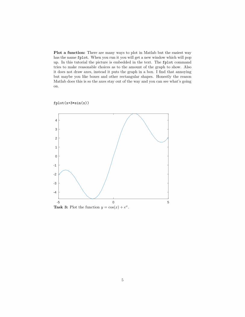
Plot a function: There are many ways to plot in Matlab but the easiest wayhas the name fplot. When you run it you will get a new window which will popup. In this tutorial the picture is embedded in the text. The fplot commandtries to make reasonable choices as to the amount of the graph to show. Alsoit does not draw axes, instead it puts the graph in a box. I find that annoyingbut maybe you like boxes and other rectangular shapes. Honestly the reasonMatlab does this is so the axes stay out of the way and you can see what’s goingon.

fplot(x+3*sin(x))

-5 0 5

-4

-3

-2

-1

0

1

2

3

4

Task 3: Plot the function y = cos(x) + ex.

5

If you want to give it a specific domain of x-values you can do that too:

fplot(x+3*sin(x),[-3,3])

-3 -2 -1 0 1 2 3

-4

-3

-2

-1

0

1

2

3

4

Task 4: Plot the function f(x) = x2 + x sinx on the interval [−2π, 2π].

6

Calculus 1

There are some other things we can do.

Take a derivative and then substitute:

subs(diff(x^3),x,3)

ans =

27

Task 5: Find the derivative of x2

x+1at x = −2.

Notice that subs is wrapped around diff. If we wrap diff around subs lookat what happens and think about why. Do you know why?

diff(subs(x^3,x,3))

ans =

0

Find an indefinite integral: Notice that Matlab, like many careless students,never puts a +C in its indefinite integrals. Grrr.

int(x*sin(x))

ans =

sin(x) - x*cos(x)

Task 6: Find∫x+ x2 tan(x) dx.

Find a definite integral:

int(x*sin(x),0,pi/6)

ans =

1/2 - (pi*3^(1/2))/12

Task 7: Find∫ 1

−1xe2x+1 dx.

7

Calculus 2

Plot a parametric curve: Plot the parametric curve x = cos t and y = sin tfor 0 ≤ t ≤ π. Note that this also a Calculus 3 problem if we think of this asplotting the VVF given by r̄(t) = cos(t)i+sin(t)j. Notice also the new symbolicvariable t is declared.

syms t

fplot(cos(t),sin(t),[0,pi])

-1 -0.5 0 0.5 10

0.1

0.2

0.3

0.4

0.5

0.6

0.7

0.8

0.9

1

Task 8: Plot the curve x = t

10cos t and y = t

5cos t for 0 ≤ t ≤ 4π.

8

Calculus 3 - Vectors

Define a vector: Vectors in Matlab are treated like in linear algebra so thismay be new to you. The vector 2i+3j+7k can be entered either as a horizontalvector or a vertical vector. Whatever you choose to use, be consistent. I will usehorizontal vectors in this guide because that’s how we think of them in Math241, except with i, j and k.

As a horizontal vector (like I’ll do) we use spaces or commas to separate values.

u=[2,3,7]

u =

2 3 7

We can put variables inside vectors too for VVFs and then take derivatives andstuff like that:

a=[t^2,1/t,2*t]

diff(a)

int(a,1,3)

a =

[ t^2, 1/t, 2*t]

ans =

[ 2*t, -1/t^2, 2]

ans =

[ 26/3, log(3), 8]

Task 9: Assign r̄(t) to be the VVF r̄(t) = t3i− etj+ k and then find r̄′(t) and∫ 2

0r̄(t) dt.

9

Combinations of Vectors

Here are various combinations of vectors. Notice also here the semicolons at theend of the first two lines. These semicolons suppress the output, meaning we’retelling Matlab ”assign the vectors and keep quiet about it”. Also note the useof norm for the length (magnitude) of a vector. Don’t use the Matlab commandlength because that just tells you how many elements are in the vector.

u=[6,9,12];

v=[-1,0,3];

norm(u)

w=u+v

dot(u,v)

cross(u,v)

dot(u,cross(u,v))

dot(u,v)/dot(v,v)*v

ans =

16.1555

w =

5 9 15

ans =

30

ans =

27 -30 9

ans =

0

ans =

-3 0 9

10

A few things to observe: The cross command produces a new vector, obviously.The second-to-last value is 0 and you should have expected that. Why? Whatis the last calculation finding? It’s something familiar.

Here’s the distance from the point (1,2,3) to the line with parametric equationsx=2t, y=-3t+1, z=5. Make sure you see what’s going on here. The point Q is offthe line, the point P is on the line and the vector L points along the line. Thereason P and Q are given as vectors is that we can then easily do Q-P to get thevector from P to Q.

Q=[1,2,-3];

P=[0,1,5];

L=[2,-3,0];

norm(cross(Q-P,L))/norm(L)

ans =

8.1193

Warning: There are certain things which behave differently in Matlab thanyou might expect because Matlab knows a bit more than you might about somethings. For example the dot product of two vectors has a more flexible definitionif the entries are complex numbers. In the above example this was never an issuesince neither u nor v is complex but if we try to use a variable look at whathappens. Notice I’ve put clear all first which completely clears out Matlabso we know we’re starting anew.

clear all;

syms t;

a=[t,2*t,5];

dot(a,a)

ans =

5*t*conj(t) + 25

What happened? Matlab doesn’t know that t is a real number and so it doesthe more generic dot product which we are not familiar with. If we want Matlabto know that t is a real number we can tell it:

clear all;

syms t;

11

assume(t,’real’);

a=[t,2*t,5];

dot(a,a)

ans =

5*t^2 + 25

That additional line assume(t,’real’) tells Matlab to treat t as a real numberso that conj stuff (complex conjugate) won’t bother us.

We can also find the norm of a symbolic vector. Here we’ll redefine our variablesfor clarity and I’ll simplify:

assume(t,’real’);

a=[t,2*t,5];

simplify(norm(a))

ans =

5^(1/2)*(t^2 + 5)^(1/2)

Task 10: Define four points P = (2,−1, 3), Q = (0, 7, 9), R = (4,−9,−3) andS = (7,−6,−6) and then with two subtractions and one dot product all on oneMatlab line show that the line through P and Q is perpendicular to the linethrough R and S.

Task 11: Define two points P = (1,−2, 3) and Q = (2,−1, 3) and one vectorn̄ = 2i+ 2j+ 3k and then with one subtraction and one dot product all on oneMatlab line show that Q is not contained in the plane containing P and normalto n̄.

Task 12: Define four points P = (5, 0, 2), Q = (1, 1, 1), R = (0, 1,−2) andS = (1,−2,−1) and then with five subtractions, two cross products and one dotproduct all on one Matlab line find the distance from S to plane containing theother three points.

12

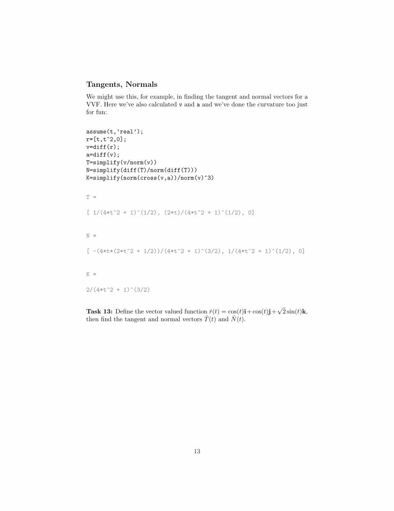
Tangents, Normals

We might use this, for example, in finding the tangent and normal vectors for aVVF. Here we’ve also calculated v and a and we’ve done the curvature too justfor fun:

assume(t,’real’);

r=[t,t^2,0];

v=diff(r);

a=diff(v);

T=simplify(v/norm(v))

N=simplify(diff(T)/norm(diff(T)))

K=simplify(norm(cross(v,a))/norm(v)^3)

T =

[ 1/(4*t^2 + 1)^(1/2), (2*t)/(4*t^2 + 1)^(1/2), 0]

N =

[ -(4*t*(2*t^2 + 1/2))/(4*t^2 + 1)^(3/2), 1/(4*t^2 + 1)^(1/2), 0]

K =

2/(4*t^2 + 1)^(3/2)

Task 13: Define the vector valued function r̄(t) = cos(t)i+cos(t)j+√2 sin(t)k,

then find the tangent and normal vectors T̄ (t) and N̄(t).

13

Plotting Points

Okay, let’s plot some stuff in three dimensions! Here is how we can plot justone point, the point (1,2,3):

view([10 10 10])

plot3(1,2,3,’o’)

00.5

11.5

2

1

1.5

2

2.5

32

2.5

3

3.5

4

14

And here are two points:

plot3(1,2,3,’o’,-1,2,5,’o’)

view([10 10 10])

-1

-0.5

0

0.5

1

1

1.5

2

2.5

3

3

3.5

4

4.5

5

Note the ’o’ tells Matlab to draw circles for points. Also note the view com-mand there. Matlab has an annoying habit of viewing the axes from a nonstan-dard angle. The view([10 10 10]) command puts our point-of-view at thepoint (10, 10, 10) so we look down at the origin as we’re used to in class.

Important observation! On the figure window there is a little rotation buttonwhich allows you to drag the picture around and look at it from different angles.Very useful and fun too! I can’t demonstrate in a fixed html document though.

Task 14: Plot the three points together (1, 2, 3), (2,−3, 0) and (−3, 5, 1).

15

Plotting Curves

Okay now, let’s plot some curves! We’ll use the 3D command fplot3. In classwe sketched a helix with r̄(t) = cos(t)i+ sin(t)j+ tk.

fplot3(cos(t),sin(t),t,[0,6*pi])

view([10 10 10])

0-1

5

-0.5-0.5

10

00

15

0.50.5

1

16

Here’s a different thing - it’s a circle but the z-value is oscillating as well, fivetimes around the circle:

fplot3(cos(t),sin(t),sin(5*t),[0,2*pi])

view([10 10 10])

-1

-0.5

-0.5-0.5

0

00

0.5

0.50.5

1

Task 15: Plot the VVF given by r̄(t) = 3 cos(t)i+ 1

tj+2 sin(t)k for 0.1 ≤ t ≤ 2π.

Task 16: Plot the VVF given by r̄(t) = ti+ tj+ (9− t2)k for −3 ≤ t ≤ 3.

17

If you have a VVF defined already and wish to fplot3 it then you need to giveit the component functions. You can do this like:

r=[t,-t,t^2];

fplot3(r(1),r(2),r(3),[-1,1])

view([10 10 10])

0-1 -1

0.2

-0.5 -0.5

0.4

0 0

0.6

0.8

0.50.5

1

11

18

Plotting Vectors

Here’s a vector in 3D. The first three coordinates are the anchor point and thelast three are the vector. So this is the vector 3i+ 4j− 2k anchored at (1, 2, 3).

quiver3(1,2,3,3,4,-2)

view([10 10 10])

daspect([1 1 1])

1

2

1.5

2

13

2.5

3

4 2

35

46This last command daspect sets the aspect ratio so that all the axes are scaledthe same. I have no idea why Matlab doesn’t do this by default but grumblegrumble grumble.

Task 17: Plot the vector 2i− 3j− 1k anchored at (−1, 4, 2).

19

Plotting Planes

Just to close out let’s draw some planes. Matlab has a great command patch

which draws a polygon. To use this to draw a plane we need to give it severalpoints on the plane. It’s a bit awkward - we need to give the points in orderaround the plane in either direction and we need to give it the x-coordinatestogether and the y-coordinates together. There’s a slick way to do the secondpart but for the first part we just need to choose the points carefully, followingaround the part of the plane we want to plot. Here are some examples.

For the plane x+2y+3z = 12 we’ve seen that we can get a good picture usingthe intercepts (12, 0, 0) and (0, 6, 0) and (0, 0, 4). The order we take them indoesn’t matter since any order will either be counterclockwise or clockwise. Todraw this with patch we do:

figure

points = [12 0 0;0 6 0;0 0 4];

patch(points(1,:),points(2,:),points(3,:),[0.95 0.95 0.95]);

view([10 10 10])

00 0

1

2 5

2

3

4 10

4

6 15

Task 18: Plot the plane 2x+ y + 4z = 16.

20

For the plane 2x+4y = 20 we’ve seen that the way to approach this is to drawthe line 2x + 4y = 20 in the xy-plane and then extend upwards. The x andy-intercepts are (10, 0, 0) and (0, 5, 0) so we’ll plot those along with (10, 0, 10)and (0, 5, 10). Note that the order we’ve chosen goes around the piece of theplane.

figure

points = [10 0 0;0 5 0;0 5 10;10 0 10];

patch(points(:,1),points(:,2),points(:,3),[0.95 0.95 0.95]);

view([10 10 10])

000

2

4

25

6

4

8

10

106

Task 19: Plot the plane 3y + 4z = 12.

Task 20: Plot the plane z = 3.

The end.

21