rotation rates of koronis family asteroid (1029) la...
TRANSCRIPT

Rotation Rates of Koronis Family Asteroid
(1029) La Plata
Alessondra Springmann
Advisor: Stephen M. Slivan
Wellesley College Department of Astronomy
May 18, 2007
For Astronomy 350, Spring 2007
– 2 –
ABSTRACT
Members of the Koronis family of asteroids have been noted for their odd
spin behavior in that these objects have “marked alignments of their spin vec-
tors, which has interesting implications for the evolution of small asteroids and
the age of the family (Slivan et al. 2007).” To expand the sample of ten objects,
the rotation periods and spin vectors of more family members need to be mea-
sured. By combining previously collected data of Koronis family member (1029)
La Plata with new observations, we can better constrain its rotation period in
addition to determining its spin vector, increasing the number of Koronis family
objects for which spin vector solutions have been performed.
1. Introduction
Asteroids, or small solar system bodies, are leftovers from the formation of our solar
system. Once referred to as “vermin of the skies” due to their unpredictable nature and
for disrupting astronomical observations of galaxies and other objects outside of the Solar
System, these bodies are now known to be scientifically interesting instead of a nuisance.
As some asteroids are mostly unchanged since their formation, studying these bodies allows
us to better comprehend the early conditions of the Solar System and therefore the Earth,
and also predict future impacts with our planet.
Asteroid families, or groupings, were first remarked upon by Hirayama (1918), and are
now widely believed to be caused by a collision between a large parent body and a smaller
asteroid. Family members tend to retain similar orbital elements to their parent body after
the disrupting collision, such as orbital eccentricity, inclination, and semimajor axis. The
Koronis family of asteroids, located in the main belt, is a Hirayama family thought to be
– 3 –
on the order of billions of years old (Bottke et al. 2001). Through laboratory and numerical
experiments, astronomers predict that the rotation rates of Koronis family members should
follow a Maxwellian distribution, in addition to having random spin orientations in space
(Bottke et al. 2006).
Koronis family members do not behave in this predicted manner: in contrast, at least
ten objects in this family demonstrate a bimodal distribution of spin vectors (Figure 1)
and appear to be trapped in spin-orbit resonances with the longitude of Saturn’s s6 orbit
node (Vokrouhlicky et al. 2003). Objects rotating in the prograde sense (i.e. rotating in the
same direction as their orbit) have periods ranging from 7.5 to 9.5 hours and obliquities
between 42◦ and 50◦, while objects rotating in a retrograde sense have rotation periods less
than 5 hours or greater than 13 hours, with obliquities greater than or equal to 154◦ (Slivan
2002; Slivan et al. 2003). These spin vectors are inconsistent with the predictions of the
laboratory model and to explain this behavior we must look at forces other than collisions.
It is assumed that this odd spin grouping is due to Yarkovsky or YORP (Yarkovsky-
O’Keefe-Radzievskii-Paddack) effects, which are thermal torques due to solar radiation
that can change the rotation rates and spin vector alignments of small bodies. Thermal
forces may cause Koronis objects to be trapped in spin-orbit resonances, where spin axes
are less likely to be perturbed by thermal radiation effects. Models by Vokrouhlicky
et al. (2003) show that the YORP effects are plausible explanations for the unexpected
bimodal alignment of these spin vectors and that YORP forces work most efficiently on
asteroids less than 40 kilometers in diameter. As the largest member of the Koronis family
is 42 kilometers across (Slivan et al. 2003), it would not be unreasonable to assume that
Yarkovsky or YORP forces are responsible for perturbing the spin axis alignment of Koronis
family objects into the present observed distribution.
Spin axis alignments of Koronis family objects are calculated by inversion of rotation

– 4 –
lightcurves to determine shape, pole, sidereal period, and sense of rotation (prograde versus
retrograde) (Slivan et al. 2003). However, there only exist models for 10 Koronis family
objects, biased against low amplitude objects or ones with longer periods (Slivan et al.
2007). Thus, in order to reduce sampling bias, more Koronis family objects need to be
observed and their spin axes determined. In this paper, we present observations of Koronis
family object (1029) La Plata from 1975 to 2007 to better constrain the sidereal rotation
period and thus eventually expand the sample of objects for which exist shape models and
pole solutions.
2. Observations & Data Reduction
In this paper, we present rotation lightcurves of Koronis family member (1029) La
Plata obtained between 1975 and 2007. Observations from 1975 were recorded at the
Kvistaberg Observatory, Uppsala-Bro, Sweden by Lagerkvist (1978) using photographic
plates and measurements were made with an iris photometer. Binzel (1987) recorded
observations at McDonald Observatory, Ft. Davis, Texas using the 0.91-m Cassegrain
telescope there and took measurements with a photoelectric photometer. The majority
of observations were recorded at Whitin Observatory at Wellesley College, Wellesley,
Massachusetts. Observations were made in the V filter with four minute integrations, using
a 1024-pixel square CCD detector with an image scale of 0.9 arcseconds per pixel and a
field size of 16’ square at Cassegrain focus. The nightly observing circumstances for the six
previously unpublished individual lightcurves are given in Table 1.
Composite lightcurve plots are shown in Figures 2-3 with the horizontal (time) axis
marked in UT hours on the date of the composite curve, covering one cycle of the rotation
period. Data from different nights have been translated into the plotted time span modulo
the given rotation period.

– 5 –
2.1. (1029) La Plata
La Plata had been previously observed by Lagerkvist (1978), Binzel (1987), and Slivan
et al. (2007). We observed La Plata during its 2007 apparition on 2007 Mar 12 and Mar 25.
The refined synodic period of 15.310 ± 0.003 h was used for folding together observations
from different nights. Daylight constraints prevented observing the entire rotation period
of (1029) in one night, so by using the known synodic period of (1029), it was possible to
determine over which time spans on a given night that the missing lightcurve portions could
be observed. Data images taken during 2007 were reduced using IRAF1 and calibrated to
standard stars using an extinction solution.
3. Results
From Slivan et al. (2007) the refined synodic period was determined to be 15.310±0.003
h, more precise than the period of 15.37 ± 0.10 h determined by Binzel (1987). Using
this synodic period, observations during one apparition were folded together to generate
a lightcurve over one rotation period. Observations taken between 2005 and 2007 are
presented in Figures 2-3. Reduced V magnitude is plotted versus UT hours on the first
night of observation during the 2005 apparition (Fig. 2) while relative V magnitude is
plotted versus hours for the 2007 apparition (Fig. 3).
Observations were corrected for the changing solar phase angle during apparitions by
using the Lumme-Bowell relation (Binzel et al. 1989). For (1029) La Plata, we assumed a
mean solar phase slope parameter of G = 0.179. For each night of observations, effects due
1IRAF is distributed by the National Optical Astronomy Observatories, which are oper-
ated by the Association of Universities for Research in Astronomy, Inc., under cooperative
agreement with the National Science Foundation.
– 6 –
to the changing solar phase angle were removed from the reduced magnitudes.
To link apparitions, the amount of time elapsed between maxima must be known in
order to correctly determine the number of rotation cycles elapsed between apparitions.
For doubly periodic lightcurves of approximately symmetric asteroids, it suffices to observe
down to half of a period in order to determine the location of lightcurve extrema.
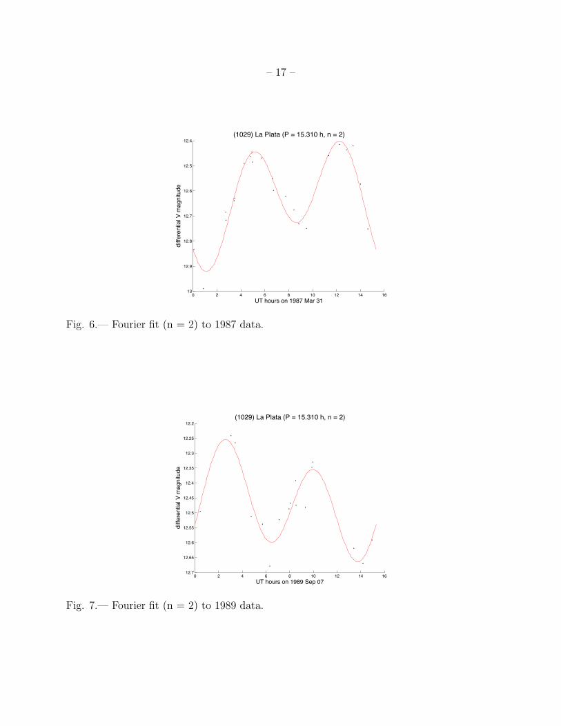
In order to best estimate the times of maxima we fit a Fourier series to the lightcurves,
then used only the constant term and the second-order harmonics to determine the times
corresponding to lightcurve maxima. In the cases where the lightcurve coverage was
insufficient to fit a doubly-period Fourier series at the synodic period, lightcurve data were
fit using half the synodic period with a singly periodic Fourier model (Slivan et al. 2003).
Both non-linear and linear least-squares fitting methods were used to plot Fourier series
on top of the observations of the 2004 apparition, yielding indistinguishable results, but as
the linear algorithm took less time computationally and did not require initial guesses as to
the fit parameters unlike the non-linear method, the linear one was used to fit data from the
rest of the apparitions (see Figures 4-10). As we were not fitting for the period, a non-linear
parameter, it was sufficient to use a linear fit to determine Fourier series coefficients.
To link apparition maxima, the time elapsed between apparitions was calculated then
divided by the lower and upper limits of the known synodic period to better constrain the
sidereal rotation period. From this, the minimum and maximum number of cycles elapsed
between two apparitions could be calculated. The difference in the ecliptic longitude of the
phase angle bisector, which determines the longitude of the point on the asteroid facing the
Earth, was also calculated.
When calculating the sidereal rotation period from the synodic period, we assume that
the same feature in the lightcurve occurs at the same part in the asteroid’s rotation, no
– 7 –
matter where Earth is relative to the asteroid. Looking at the asteroid from Earth, it makes
most sense to measure the rotational phase relative light reflected normal to the surface of
the asteroid at a specific point (Figure 11).
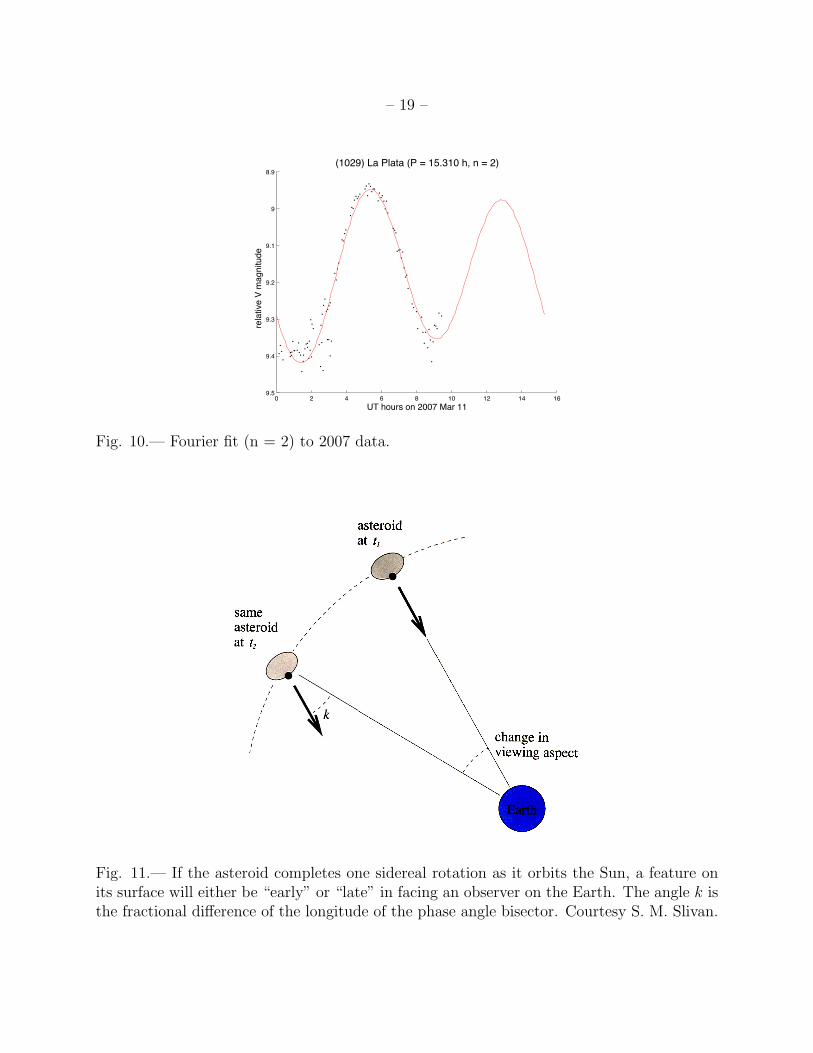
Between t1 and t2, observers on Earth see a point (with a specific longitude of the phase
angle bisector) on the surface of the asteroid revolve less than 360◦ about the asteroid’s axis
if the asteroid is rotating prograde, but more than 360◦ if the asteroid is rotating in the
retrograde sense. In this figure if the asteroid is spinning prograde, it has to rotate some
distance more to complete its 360◦ rotation whereas for rotating in the retrograde sense,
it has already completed one full rotation and thus arrived “early” as seen by an observer
on Earth measuring the change in phase angle bisector. The angle k is the difference in
longitude of the phase angle bisector—if the asteroid is late, it will have to rotate through
this angle k for the same point on its surface to face Earth again whereas if the asteroid is
early, it will have already rotated through this angle k past 360◦.
By determining what fraction of an orbit the asteroid has already completed or has yet
to complete between apparitions based on its orbital position and change in the longitude of
the phase angle bisector, the number of cycles elapsed can be constrained based on whether
the asteroid is rotating in either a prograde or retrograde sense. When determining the
change in phase of a lightcurve maxima, we assume that the the asteroid is spinning with
its pole normal to the plane it makes with the Earth. The times of maxima and longitude
of the phase angle bisector are shown in Table 2.
The fraction of turns the asteroid would have to complete to face Earth again, combined
with the number of cycles elapsed between features, can be used to calculate a new sidereal
period for rotation in either the prograde or retrograde sense and eventually constrain these
values. The error in the sidereal period is equivalent to the inverse of the number of cycles
elapsed, so as the sidereal period is calculated between apparitions that are further and

– 8 –
further away from each other are used, the error in the sidereal period decreases. Table 3
shows the fractional change in the phase angle bisectors between apparitions while Table 4
shows the calculated sidereal period between apparitions.
The refined sidereal period is sufficient to link the 1975 and the 1983 apparitions, which
are six apparitions apart. Even though the periods appear to be converging in both the
retrograde and prograde sense, it was impossible to determine whether (1029)’s rotation
sense was prograde or retrograde.
Given the possible range of cycles elapsed between the 1975 and 1983 apparitions
(between 4301.38 and 4301.53 cycles), the only period that is consistent with the fractional
change in the phase angle bisector (0.46 or 0.96 if retrograde; 0.04 or 0.54 if prograde)
is the sidereal period corresponding rotation in the retrograde sense, providing a value of
15.3110 ± 0.0002 hours for the sidereal period. If the asteroid was rotating in a prograde
sense, the fractional change in the longitude of the phase angle bisector would be 0.01
rotations larger than the upper bound of the number of cycles elapsed, whereas if the
asteroid is rotating in a retrograde sense, the fractional change of the phase angle bisector
falls comfortably within the range of possible cycles elapsed.
4. Conclusion
Calculating the sidereal period from the synodic rotation period of (1029) La Plata
using the time elapsed between apparitions yields a retrograde period of 15.3110± 0.0002 h,
slightly larger than the synodic period of 15.310± 0.003 h calculated by Slivan et al. (2007)
and consistent with the other calculated sidereal periods between apparitions (as shown in
Table 4).
For Koronis family objects with existing shape solutions and known polar alignments,

– 9 –
objects that rotate in the retrograde sense have rotation periods less than 5 hours or greater
than 13 hours (Slivan 2002; Slivan et al. 2003; Bottke et al. 2006). This calculated sidereal
period seems consistent with other retrograde Koronis family objects, though the possibility
remains that this object is rotating in the prograde sense, as the prograde sidereal period
is 0.01 rotation cycles away from the range of elapsed cycles between apparitions for which
this sidereal period was calculated.
Regardless, the pole orientation and thus the spin vector direction of (1029) La Plata
is not yet known. The sidereal rotation period was calculated assuming that the asteroid’s
rotation vector is normal to the plane between the asteroid and the Earth; knowing the true
pole alignment would thus change the number of elapsed cycles and thus the calculated
period of (1029). There exist a number of methods in the literature (Slivan et al. 2003) that
can further refine the sidereal period in addition to calculating the spin vector orientation of
(1029). Only when the shape model and spin vector of (1029) La Plata are known can it be
determined whether this object fits into the known distribution of Koronis family objects.
More Koronis family members must be observed to expand upon the sample with
known spin vectors and shape solutions to determine whether the behavior of this small
sample is indicative of the spin alignments of the rest of the family. Understanding Koronis
family rotation dynamics not only gives us a better understanding of the formation of this
family, but a better comprehension of the implications of Yarkovsky and YORP effects
acting not only on Koronis family objects but on other bodies in the Solar System.

– 10 –
Acknowledgments
I am grateful to Professor Slivan for his guidance, patience, encouragement, and
knowledge; for Tim Smith’s ability to convince Matlab to parse text; for Kate and Bekki’s
keeping the asteroids in check; for Dick French reminder about Julian dates; and for the
rest of the Astronomy Department’s support.

– 11 –
REFERENCES
Binzel, R. P. 1987, Icarus, 72, 135
Binzel, R. P., Gehrels, T., & Matthews, M. S., eds. 1989, Asteroids II (The University of
Arizona Press)
Bottke, W. F., Vokrouhlicky, D., Broz, M., Nesvorny, D., & Morbidelli, A. 2001, Science,
294, 1693
Bottke, Jr., W. F., Vokrouhlicky, D., Rubincam, D. P., & Nesvorny, D. 2006, Annual
Review of Earth and Planetary Sciences, 34, 157
Hirayama, K. 1918, AJ, 31, 185
Lagerkvist, C.-I. 1978, A&AS, 31, 361
Slivan, S. M. 2002, Nature, 419, 49
Slivan, S. M., Binzel, R. P., Boroumand, S. C., Pan, M. W., Simpson, C. M., Tanabe, J. T.,
Villastrigo, R. M., Yen, L. L., Ditteon, R. P., Pray, D. P., & Stephens, R. D. 2007,
Icarus
Slivan, S. M., Binzel, R. P., Crespo da Silva, L. D., Kaasalainen, M., Lyndaker, M. M., &
Krco, M. 2003, Icarus, 162, 285
Vokrouhlicky, D., Nesvorny, D., & Bottke, W. F. 2003, Nature, 425, 147
This manuscript was prepared with the AAS LATEX macros v5.0.

– 12 –
Tables
Table 1: Observing circumstances for (1029) La PlataUT date α◦ Filter Telescope Observer(s) Fig.
2005 12 04.1 2.8 V Whitin Observatory 0.61-m Springmann 212 08.1 1.3 V Whitin Observatory 0.61-m Maynard 212 09.0 1.1 V Whitin Observatory 0.61-m Slivan 212 10.1 0.9 V Whitin Observatory 0.61-m Slivan 2
2007 03 12 1.2 V Whitin Observatory 0.61-m Springmann 303 26 5.1 V Whitin Observatory 0.61-m Springmann 3
Table 2: Times of maximaYear Reference Day Time of First Maximum λPAB
(hours after 0 UT) (◦)
1975 Nov 07 0.16 033.21983 May 13 4.40 228.41987 Mar 31 4.89 141.51989 Sep 07 2.45 327.92004 Sep 11 6.37 349.82005 Dec 04 4.93 078.22007 Mar 12 5.40 172.9

– 13 –
Table 3: Rotations elapsed between apparitionsYear range Apparitions elapsed Cycles elapsed Fractional difference of λPAB
2005 - 2004 1 703 0.251987 - 1989 2 1396 0.521983 - 1987 3 2222 0.761983 - 1989 5 3619 0.281975 - 1983 6 4301 0.54
Table 4: Calculation of sidereal periodsYear range Apparitions elapsed Calculated sidereal period
if retrograde (h) if prograde (h)
2005 - 2004 1 15.3103± 0.0014 15.3101± 0.00141987 - 1989 2 15.3106± 0.0007 15.3110± 0.00071983 - 1987 3 15.3109± 0.0004 15.3108± 0.00041983 - 1989 5 15.3110± 0.0002 15.3106± 0.00021975 - 1983 6 15.3110± 0.0002 15.3106± 0.0002

– 14 –
Figures
Fig. 1.— Shape models and north pole directions of 10 Koronis family members with spinvector determinations from Slivan (2002) and Slivan et al. (2003).

– 15 –
0 2 4 6 8 10 12 14 16
10.9
10.95
11
11.05
11.1
11.15
11.2
11.25
UT hours on 2005 Dec 04
diffe
rent
ial V
mag
nitu
de
(1029) La Plata (P = 15.310 h)
Fig. 2.— Observations from 2005 courtesy of S. M. Slivan.
0 2 4 6 8 10 12 14 16
8.9
9
9.1
9.2
9.3
9.4
9.5
UT hours on 2007 Mar 11
rela
tive
V m
agni
tude
(1029) La Plata (P = 15.310 h)
Fig. 3.— Observations from 2007.

– 16 –
0 2 4 6 8 10 12 14 16
!4.2
!4.1
!4
!3.9
!3.8
!3.7
!3.6
!3.5
!3.4
UT hours on 1975 Nov 07
diffe
rent
ial V
mag
nitu
de
(1029) La Plata (P = 15.310 h, n = 1)
Fig. 4.— Fourier fit (n = 1) to 1975 data.
0 2 4 6 8 10 12 14 16
11.7
11.8
11.9
12
12.1
12.2
UT hours on 1983 May 13
diffe
rent
ial V
mag
nitu
de
(1029) La Plata (P = 15.310 h, n = 1)
Fig. 5.— Fourier fit (n = 1) to 1983 data.
– 17 –
0 2 4 6 8 10 12 14 16
12.4
12.5
12.6
12.7
12.8
12.9
13
UT hours on 1987 Mar 31
diffe
rent
ial V
mag
nitu
de
(1029) La Plata (P = 15.310 h, n = 2)
Fig. 6.— Fourier fit (n = 2) to 1987 data.
0 2 4 6 8 10 12 14 16
12.2
12.25
12.3
12.35
12.4
12.45
12.5
12.55
12.6
12.65
12.7
UT hours on 1989 Sep 07
diffe
rent
ial V
mag
nitu
de
(1029) La Plata (P = 15.310 h, n = 2)
Fig. 7.— Fourier fit (n = 2) to 1989 data.

– 18 –
0 2 4 6 8 10 12 14 16
10.8
10.9
11
11.1
11.2
11.3
11.4
11.5
11.6
11.7
11.8
UT hours on 2004 Sep 11
diffe
rent
ial V
mag
nitu
de
(1029) La Plata (P = 15.310 h, n = 7)
Fig. 8.— Fourier fit (n = 7) to 2004 data.
0 2 4 6 8 10 12 14 16
10.9
10.95
11
11.05
11.1
11.15
11.2
11.25
UT hours on 2005 Dec 04
diffe
rent
ial V
mag
nitu
de
(1029) La Plata (P = 15.310 h, n = 4)
Fig. 9.— Fourier fit (n = 4) to 2005 data.
– 19 –
0 2 4 6 8 10 12 14 16
8.9
9
9.1
9.2
9.3
9.4
9.5
UT hours on 2007 Mar 11
rela
tive
V m
agni
tude
(1029) La Plata (P = 15.310 h, n = 2)
Fig. 10.— Fourier fit (n = 2) to 2007 data.
Fig. 11.— If the asteroid completes one sidereal rotation as it orbits the Sun, a feature onits surface will either be “early” or “late” in facing an observer on the Earth. The angle k isthe fractional difference of the longitude of the phase angle bisector. Courtesy S. M. Slivan.