rotor loads prediction using helios: a multi-solver

Rotor Loads Prediction Using Helios: A Multi-Solver

Framework for Rotorcraft CFD/CSD Analysis

Jayanarayanan Sitaraman∗ 1, Mark Potsdam† 2, Buvaneswari Jayaraman‡ 3, AnubhavDatta§ 3, Andrew Wissink¶ 2, Dimitri Mavriplis‖ 1, and Hossein Saberi∗∗ 4

1University of Wyoming, Laramie, WY2U.S. Army Aeroflightdynamics Directorate (AMRDEC), Moffett Field, CA

3NASA Ames Research Center, Moffett Field, CA4Advanced Rotorcraft Technologies, Sunnyvale, CA

We explore the use of the Helios high-fidelity rotorcraft simulation software for forwardflight CFD/CSD simulation of the UH-60A rotorcraft, comparing computed results forthree critical flight conditions. The approach used for moving-body CFD/CSD analysis inHelios applies Cartesian-based unsteady adaptive mesh refinement (AMR) for the off-bodywake solution, and results with the enhanced wake solution are compared to traditionalfixed off-body refinement. Results show airload predictions that are generally comparableto existing state-of-the-art CFD/CSD analysis codes. The enhanced wake resolution fromAMR provides some improvement to vibratory airload predictions but the improvementsare marginal.

I. Introduction

This paper presents a validation of the aerodynamic loading predictions of the UH-60A Black Hawk rotor-craft using the multi-solver rotorcraft CFD/CSD analysis framework – Helios. Helios1 is being designed anddeveloped by the DOD-sponsored High Performance Computing (HPC) institute for Advanced RotorcraftModeling and Simulation (HIARMS). Improvement of usability, accuracy and efficiency were the principalmetrics utilized in the design and development of Helios. To this end, Helios provides several novel fea-tures that are different from existing state-of-the-art. These include (1) a multi-code unstructured/Cartesiandual-mesh CFD solver architecture,2 (2) an automated and parallel overset grid assembling capability withimplicit hole-cutting3 (3) the capability for solution adaption and high-order accuracy in the off-body solver4

(4) an unstructured patch force based fluid-structure interface5 and (5) a Python-based software integrationframework that supports seamless and efficient data exchange between component modules.6

The fluid dynamics model in Helios differs from traditional monolithic CFD code architecture owing toits utilization of a heterogeneous meshing paradigm (Fig. 1). The meshing paradigm in Helios combines theadvantages of unstructured grids (their ability to model complex geometry, resolving boundary layers usinganisotropic meshes) and Cartesian adaptive grids (efficient high order algorithms, efficient storage, ease ofsolution based adaption). The use of multiple mesh paradigms provides the potential for optimizing thegridding strategy on a local basis. For the rotorcraft problem in particular, it is apparent that one shouldemploy body fitted unstructured grids around the solid boundaries and then transition the gridding paradigmto solution adaptive Cartesian grids for wake capturing. The use of a heterogeneous meshing paradigm doesinvolve several implementation challenges. For example, integrating different meshing paradigms into a

∗Assistant Professor, Dept. Mechanical Engineering, AIAA Member†Aerospace Engineer, Research Development and Engineering Command, AIAA Member‡Research Scientist, Science and Technology Corp.,§Research Scientist, Science and Technology Corp.,¶Aerospace Engineer, Research Development and Engineering Command, AIAA Member‖Professor, Dept. Mechanical Engineering, AIAA Member

∗∗Vice President

1 of 35

American Institute of Aeronautics and Astronautics

Figure 1. Overset near/off-body gridding paradigm used in Helios. Unstructured or curvilinear grids to capturegeometric features and boundary layer near body surface, adaptive block-structured Cartesian grids to capture far-fieldflow features.

single large monolithic code is complex and has the disadvantage of forcing at least one of the griddingparadigms to be less optimized and flexible than the original stand alone solver. In Helios, we overcomethis challenge by utilizing a multiple-mesh strategy that is implemented through the use of multiple CFDcodes, each optimized for a particular mesh type. In addition to supporting heterogeneous grids and solvers,the software was also developed in a manner to minimize the analysis burden on the user. While an interfaceprocedure is required for each specific solver, this interface must only be written once. Once the interfaceexists, the domain connectivity software retrieves the information it needs directly from the flow solvers andthe grids themselves, so the human analyst does not need to provide input specific to each problem. Thedesign paradigm used in Helios automates most analysis procedures, thus considerably simplifying its routineusage for production needs. For example, for the four-bladed UH-60A simulation, the only grid generationrequired is for a single blade (i.e. the user needs to create an unstructured grid that extends about one chordfrom the blade). The creation and partitioning of the four-bladed grid system, the generation/adaption ofthe off-body Cartesian grid system, the execution of the overset grid assembly, the execution of CFD/CSDcoupling and data exchange are completely automated from then on and can proceed seamlessly withoutany user intervention.

The focus of this paper concerns primarily the prediction of aerodynamic loading and resolution of thevortex wake structure. We utilize the UH-60A flight test data obtained as part of the UH-60A airloadsprogram (jointly sponsored by NASA and the U.S. Army) for all the validation and verification purposes.The flight test data set is quite comprehensive and contains measurements of rotor performance, sectionalaerodynamic loading, structural loads, blade motion, control loads and aircraft states. It also spans anextensive range of flight conditions, including level flight and maneuvers. We choose three critical flightconditions for validation/verification purposes in this paper. They are (1) steady high speed forward flight(noted henceforth as C8534 based on the test data counter label) (2) low speed transition flight (C8513) and(3) high-altitude stall flight (C9017). Coupled fluid/structure simulations for these flight conditions havebeen performed for these flight conditions by several research groups with varying degrees of success (seereferences7,9, 10). The objectives of this paper are (1) to verify that the prediction capabilities of Helios areon par with the existing state-of-the-art (2) demonstrate solution/geometry based dynamic off-body meshadaption capability in the complex operating condition involving unsteady flows and elastically deformingmeshes and (3) characterize the improvements in efficiency and accuracy brought forth by the dynamic meshadaption.

2 of 35


II. Technical Approach

Full fluid/structure coupled analysis requires the invocation of all the participant modules in Helios.These are (a) the parallel NSU3D code11 as the unstructured near-body solver (b) the SAMARC code4 whichcombines the SAMRAI framework12 and high-order ARC3DC code as the off-body solver (c) the paralleldomain connectivity module PUNDIT3 (d) a patch force based fluid/structure interface (RFSI5) and (e)the RCAS13 rotorcraft comprehensive analysis which performs structural dynamic analysis and trim. Thecoupling of all these components is accomplished through a Python-based infrastructure with emphasis onpreserving the modularity of the participating solvers. In addition to the advantages in efficiency and easein code development, coupling existing mature simulation codes through a common high-level infrastructureprovides a natural way to reduce the complexity of the coupling task and to leverage the large amount ofverification, validation, and user experience that typically go into the development of each separate model.Brief descriptions of the implementations of all the component modules and the python infrastructure areoutlined below. More detailed descriptions and validations of the Python-based infrastructure can be foundin Refs.2,6

II.A. Python Infrastructure

Python-based computational frameworks have been developed previously by other researchers14 as ameans of coupling together existing legacy codes or modules. Such a framework has a number of advantagesover a traditional monolithic code structure: (1) it is easier to incorporate well-tested and validated legacycodes rather than to build the capabilities into an entirely new code, (2) there is less code complexity inthe infrastructure itself, so maintenance and modification costs are less, and (3) it is easier to test andoptimize the performance of each module separately, often yielding better performance for the code as awhole. Essentially, Python enables the legacy solvers to execute independently of one another and referenceeach other’s data without memory copies or file I/O. Further, the Python-wrapped code may be run inparallel using pyMPI or myMPI, with each of the solvers following its native parallel implementations.

II.B. Flow Solver

The flow solution methodology in Helios utilizes a heterogeneous meshing paradigm consisting of un-structured near-body grids and Cartesian off-body grids. Three distinct modules operate synchronously tofacilitate the flow solution procedure. The modules are termed as the near-body-solver, the off-body solverand the domain connectivity module, respectively. In the following sections, we provide brief descriptions ofthe meshing paradigm and each of the participating solvers.

II.B.1. Meshing Paradigm

The meshing paradigm consists of separate near-body and off-body grid systems. The near-body gridtypically extends a short distance from the body, sufficient to contain the boundary layer. This grid can bean unstructured tetrahedral or prismatic grid that has been extracted from a standard unstructured volumegrid or generated directly from a surface triangulation using hyperbolic marching. The reason for usingunstructured grids in the near-body region is to properly capture the geometry and viscous boundary layereffects, which are difficult or impossible to capture with Cartesian grids alone. We further note that eitherstructured or unstructured grids will work equally well in the near-body region from the point of view of ourinfrastructure. Away from the body the near-body grid solution is interpolated onto a Cartesian backgroundmesh with the aid of the domain connectivity algorithm (see section II.B.4). This transition normally occursat a distance wherein the sizing of the near-body grid cells is approximately commensurate with the sizingof the Cartesian mesh in the off-body region.

The off-body grid system consists of a hierarchy of nested refinement levels, generated from coarsest tofinest. In the Structured Adaptive Mesh Refinement (SAMR) paradigm,15 the coarsest level defines thephysical extents of the computational domain. Each finer level is formed by selecting cells on the coarserlevel and then clustering the marked cells together to form the regions that will constitute the new finerlevel. Solution-based refinement progresses as follows: physical quantities and gradients are computed ateach Cartesian cell using the latest available solution and those cells that hold values deemed to requirerefinement are marked. The marked cells are then clustered to form the new set of patches that constitutethe next finer level. The process is repeated at each new grid level until the geometry and solution features

3 of 35


Figure 2. Block structured AMR grid composed of a hierarchy of nested levels of refinement. Each level containsuniformly-spaced logically-rectangular regions, defined over a global index space.

are adequately resolved. We note that this entire procedure is automated within the software and no userintervention is required. The procedure of adaptive mesh refinement is graphically illustrated in Figure 2.

An example of the overset near-body/off-body meshing strategy is given in Figure 1, which shows themeshes for flow computations over a helicopter fuselage and blade. Here, the mixed-element unstructurednear-body grid envelops the surface of the fuselage and blade, while a multi-level Cartesian off-body gridextends from the outer boundary of the near-body grid to the far-field boundary. The two sets of meshesoverlap in the so-called fringe region, where data are exchanged between the grids.

II.B.2. Near-body solver

For the unstructured solver in the near-body region, we employ the NSU3D11 code, which is an implicitnode-centered Reynolds-Averaged Navier-Stokes (RANS) code capable of handling arbitrary unstructuredmesh elements. NSU3D utilizes a node-centered finite-volume scheme, that is spatially second-order accurate.Time-accurate computations utilize second-order accurate backwards-Euler time-stepping along with dual-time-stepping for iterative convergence of the non-linear problem at each physical time-step. The solutionscheme is comprised of a non-linear multigrid algorithm that employs a three-stage Runge-Kutta schemewith line-Jacobi relaxation as a smoother at each grid level. The code employs an edge-based data structure,which facilitates flux computations on the edges of the median-dual control volume. NSU3D has beenextensively tested and benchmarked in stand-alone mode (see refs16,17).

II.B.3. Off-Body Flow Solver

The off-body solver is an Euler equation derivative of the ARC3D code,18 that is optimized for isotropicCartesian grids. It uses an explicit 3rd-order Runge-Kutta time-integration scheme and has spatial differ-encing options ranging from second- to fifth-order accurate. As mentioned earlier, the code is compiled asa library that is callable by SAMRAI, which is responsible for the overall management of the off-body gridgeneration, adaption, parallel domain decomposition and load balancing. The combined SAMRAI/ARC3Dpackage is referred to as SAMARC.4

II.B.4. Overset Methodology and domain connectivity module

The overall solution procedure for the overset meshes is as follows. At each iteration step, the solutionsof the fluid equations in each mesh system are obtained independently with the solution in each fringe regionbeing specified by interpolation from the overlapping “donor” mesh as a Dirichlet boundary condition. Atthe end of the iteration, the fringe data are exchanged between the solvers so that the evolution of theglobal solution is faithfully represented in the overset methodology. Further, if one or more of the meshesis moving or changing, the fringe regions and the interpolation weights are recalculated at the beginning of

4 of 35


the time step. For a steady-state calculation, this procedure is repeated for each iteration step until solutionconvergence is attained in both the near- and off-body meshes.

The domain connectivity module (PUNDIT3) is responsible for performing all the overset grid assem-bly operations. These include determination of donor-recipient relationships and appropriate interpolationschedules between multiple overlapping meshes. For static meshes, these operations are done once, at thebeginning of the computation, while, for the more general case of moving or adapting meshes, the determi-nations of donors and weights has to be repeated within the time-stepping or iteration loop.

All the overset grid assembly operations are fully automated and do not require any geometry inputfrom the user. In addition, PUNDIT performs all the domain connectivity operations on the partitionedgrid system in a fully parallel environment. PUNDIT adopts the implicit hole cutting procedure followedby NAVAIR-IHC.19 The core idea of this approach is to retain the grids with the finest resolution at anylocation in space as part of the computational domain and interpolate data at all coarser grids in this regionfrom the solution on the fine grid. This results in the automatic generation of optimal holes without any userspecification as in the case of explicit hole-cutting. Moreover, the implicit hole-cutting procedure producesan arbitrary number of fringe points based on mesh density compared to traditional methods which use afixed fringe width (usually single or double). The critical parameter that quantifies the quality of a gridcell or node is termed as “resolution capacity”. PUNDIT nominally uses the cell volume as the resolutioncapacity for a grid cell and the average of cell volumes of all associated grid cells as resolution capacity fora grid node. The near-body to near-body and near-body to off-body domain connectivity procedures areseparated in PUNDIT to facilitate automatic off-body grid generation and to improve efficiency (Ref.20).

II.C. Comprehensive Analysis and Fluid/Structure Interface

Accurate modeling of the UH-60 requires establishing a trim condition where all rotor aerodynamic forcesare balanced. A structural model is also needed to properly model the structural dynamics of the flexiblerotor. These structural dynamics and trim operations are provided by a rotorcraft comprehensive analysispackage that is called by Helios. That is, at each timestep Helios computes the aerodynamic loads using thedual-mesh CFD analysis and then calls the comprehensive analysis package which sets the rotor pitch angle,structural deflections, etc. Aerodynamic loads computed by CFD are transmitted to the comprehensivepackage through a fluid/structural interface. This section discusses details of this procedure.

II.C.1. Rotorcraft Comprehensive Analysis System

Rotor structural dynamics and trim coupling are handled by the Rotorcraft Comprehensive AnalysisSystem (RCAS).13 RCAS is a rotorcraft comprehensive analysis (CA) platform developed and maintained bythe U.S. Army Aeroflightdynamics Directorate (AFDD) in partnership with Advanced Rotorcraft Technology,Inc. over the past ten years. In general, RCAS contains state-of-the-art multibody, large deformation,composite nonlinear beam finite-element modeling (FEM), full aircraft trim and vehicle dynamics, andlower-order unsteady lifting-line aerodynamic models. It also contains a suite of solution procedures for levelflight trim solution, flutter and aeroelastic stability, ground/air resonance capabilities, unsteady maneuvers,and external slung load/missile release capabilities. In Helios, the RCAS component supplies the CSD andtrim modules. Importantly, it provides the delta-coupling capability that is central to multi-disciplinaryCFD-CA coupled analysis. Additional capabilities such as tight-coupling, multiple rotors and rotor-fuselageconfigurations will be included in future versions of Helios. RCAS uses a Hilbert-Hughes-Taylor timemarching with an azimuthal time step of ∆ψ = 5◦. The RCAS trim model used for these calculations isa shaft fixed, moment trim, targeting the estimated thrust and measured hub moments from the standardAirloads database, to calculate the rotor control pitch angles.

II.C.2. Fluid/structure interface

The rotor fluid-structure interface (RFSI) transfers surface forces from the near-body CFD solver tothe structural dynamic model of the rotor. The implementation is based on the exact coupling methoddescribed in Ref.5 The method consists of a patch force based interface and a modified delta procedure.The interface does not require 2-D sectional airloads from CFD, and instead, imposes each and every surfaceforce (integrated fluid stresses over surface elements) on the structure by an exact calculation of virtual work.Thus, it is both exact (conservative in energy and preservative in total airloads) and generic (applicable

5 of 35


to arbitrary grids, geometries, and structural models). The modified delta procedure also bypasses therequirement for 2-D sectional airloads and implements the delta-quantities directly at the finite elementlevel (of the structure). The patch force interface can be collapsed, as an option, on to a reduced set ofspan-wise points to re-create sectional airloads. In this form, the interface (no longer conservative but stillpreservative) allows the implementation of the conventional delta procedure. It is this form which is usedhere for coupling with RCAS.

The reduced interface provides an efficient sectional airloads calculation, without the need for this cal-culation in the CFD code itself. An example is shown in Figure 3 (from Ref.5). Figure 3(a) shows typicalpatch forces at zero azimuth for a high-speed forward flight case from a structured CFD solver. The beamexcitations from each patch force – accumulated on a limited number of span-wise points (say x) on thebeam axis (Figure 3(b)) by simply distributing them proportionally among two neighboring points aroundthe span-wise station to which it is assigned – if divided by ∆x provide an estimate of sectional airloads. Theonly difference is that whereas the sectional airloads contain only the sectional pressure/shear solution, thereduced airloads contain all patch forces within a domain (Figure 3(b)). As the number of span-wise pointsincrease, the reduced airloads approach sectional airloads. An example is shown in Figure 3(c) where thepatch forces have been accumulated on a set of 27 span-wise points (with a point at 96.5% R). The isolatedexample shown here uses a structured near-body CFD to serve the purpose of a consistent verification. Thecoupled solutions in the rest of the paper use unstructured near-body CFD.

RFSI ensures consistency of geometry and coordinate system frames between CFD and CSD solvers.Currently, the module works for conventional single rotor configurations, although the capability to handlemulti-element rotors (advanced geometry and flaps) and multiple rotor configurations is under development.

II.C.3. Mesh Motion Module (MMM)

The final component that plugs into Helios are the mesh motion and deformation modules. There aretwo specific sub-modules: pydeform which is used for prescribed motion cases, and rdeform which is usedfor full aero-elastic coupling. In both instances, the module uses the original mesh coordinates and movesand deforms the mesh to account for rotor rotation and blade surface deformations based on the azimuthaland radial location of a grid point.

II.C.4. CFD-CA Delta Coupling Analysis

The delta-coupling or loose-coupling formulation23 takes advantage of the periodic nature of the rotordynamics. In this scenario, the aerodynamic forces on the blade are obtained over a period and input intothe comprehensive analysis code. In turn, the periodic deflections are used to deform and move the mesh forthe aerodynamic simulations over the next period. This sequence of CFD and CA simulations is repeateduntil the load and deflections converge to a periodic steady-state, thereby ensuring time-accuracy of theresponse harmonics and, simultaneously, trim. In practice, the coupling is performed every N time steps ofthe CFD time-marching solution, where N is sufficient to construct airloads over one entire rotor revolutionusing the solution from all blades. These deflections are used to move the grid over the next period of rotorrevolution and so on until the loads and deflections converge.

III. UH-60 Black Hawk

III.A. Flight test data

A unique and extensive flight test database exists for a UH-60A Black Hawk helicopter in level flight andtransient maneuvers.22 The data were obtained during the NASA/Army UH-60A Airloads Program. Thedatabase provides aerodynamic pressures, structural loads, control positions, and rotor forces and moments,allowing for the validation of both aerodynamic and structural models. The test matrix contains a rangeof advance ratios and gross weight coefficients, as shown in Figure 4, with the test points investigated hereindicated. Absolute pressures were measured at r/R = 0.225, 0.40, 0.55, 0.675, 0.775, 0.865, 0.92, 0.965, and0.99 (Figure 5) along the blade chord and integrated to obtain normal force, pitching moment, and chordforce.

The data have undergone a significant amount of careful investigation,21 however, some discrepancieshave not yet been resolved. Measured rotor thrust was determined from the gross weight of the helicopter

6 of 35


0 0.2 0.4 0.6 0.8 1−5

0

5

10

15

span, r/R

lbs

Fz − vertical(total 6040)

Fy − inplane(−1130)

Fx − Axial(−478)

(a) CFD surface patch forces on a blade at ψ = 0◦; Fx is to tip,Fz is in direction of thrust; Fy is to leading edge (for counterclock-wise rotation).

(b) A limited set of span-wise points on CSD beam axis.

0 90 180 270 360360−120

−80

−40

0

4040

Azimuth, degs.

ft−lb

/ft

SectionalReduced

(c) Accumulated airloads from reduced interface (patch forcescollapsed on to a set of CSD beam axis points) compared withsectionally integrated 2-D airloads; pitching moment (1/4-c) at96.5% R.

Figure 3. Calculation of 1-D beam excitation from 3-D CFD surface forces; Verification of an exactpatch force interface by reduction on to a limited set of span-wise points and comparison with 2-Dsectional airloads.

7 of 35


Figure 4. UH-60 test matrix

Figure 5. UH-60 blade with pressure sensor locations

8 of 35


plus estimates for the fuselage and tail rotor loads. Measured hub moments, roll and pitch, were determinedfrom an upper shaft bending moment gauge. However, integration of the measured pressures over the rotorresults in poor agreement with measured thrust and moments. For example, for the high speed test point,the integrated thrust is 10% higher and the total integrated hub moment is 50% larger with an 80-degreephase difference compared to the measured values. Consequently, it is clear that there is some uncertaintyin the aircraft trim condition, and there will be some discrepancy in comparison of mean airloads values.Errors in the blade pressures can have large effects on integrated section pitching moments. Faulty trailingedge pressure taps have been discovered in this dataset that considerably skew the pitching moment meanvalues. For this reason, all plots of pitching moment have the mean removed.

The UH-60A master input database, available to approved researchers, has been used to define the elasticUH-60A four-bladed rotor model. The database contains geometric, aerodynamic, and structural materialproperties. Figure 5 shows the blade planform and pressure transducer locations. The blade has a radiusof 322 inches, and the 20 deg swept tip begins at r/R = 0.929. The solidity (blade area/disk area) σ is.0826 with a root cut-out of 14% and there is about 16 degs of nonlinear twist. The chord of the unsweptportion of the blade is 20.76 inches. The nominal rotor speed is 258 RPM. Further details of the blade canbe found in Ref.21 The geometry and grids have been developed from CAD-based surface grid definitions inPLOT3D format distributed to the UH-60 Airloads Workshop participants by Sikorsky Aircraft in 2010. Incomparison with previous theoretical definitions of the UH-60 blade,22 the CAD-based definition corrects thetab location, strings the airfoils along the span more correctly, and modifies a small region at the tip. Noneof the major blade characteristics (twist, chord, airfoil sections, planform) are changed from that used in alarge range of previous investigations. Three flight conditions are analyzed in the paper, shown in Table 1.

Table 1. UH-60 flight conditions. RM=rolling moment, PM=pitching moment, AOA=angle of attack.

Flight Advance Hover AOA Density Weight Thrust Torque Hub RM Hub PMCond Ratio Tip Mach (deg) (slug/ft3) coeff/σ coeff/σ coeff/σ (ft-lb) (ft-lb)8534 0.368 0.642 -7.31 0.0020823 0.079 0.084 0.00905 1510 -10428513 0.153 0.638 +0.75 0.0021717 0.079 0.076 0.00384 239 -13679017 0.237 0.666 -0.19 0.0013242 0.135 0.126 0.01058 97 34

IV. Computational Details

IV.A. Near-body Unstructured Grid Generation

Two unstructured near-body grids of the UH-60 blade have been used in this work, a coarse grid andfine grid. The relevant sizes of the two grids are detailed in Table 2. Both grids were generated in the samemanner. A surface grid was developed using the commercial GRIDGEN/Pointwise software, and a volumegrid based on this surface grid was created using AFLR3 from Mississippi State University. The coarse surfacemesh uses a structured mesh on the main part of the blade with fully unstructured tip caps (Figure 6(a)).The fine surface mesh uses a quasi-structured approach (Figure 6(b)), where structured cells are generatedfrom the leading edge aft and the trailing edge forward. They are then transitioned to triangles after somedistance where the cells become isotropic. In both cases, the volume grid generation process converts thequadrilateral surface cells into two triangles. The volume meshes are comprised of prismatic cells in theboundary layer and tetrahedral cells in the farfield, with some pyramidal cells for transition (Figures 6(c)and (d)). The purpose of initially developing structured grids on the surface is to allow for anisotropic cellsand stretching, which is not generally available from unstructured surface mesh generators. For the viscousboundary layer, the initial wall normal spacing on both grids is 5e-05 inches (y+ < 1). The outer boundaryspacing and distance for each grid relative to the rotor chord are also shown in Table 3. For the fine mesh, autility has been used to trim the original outer boundary back (Figure 6(f)), resulting in an irregular outerboundary compared with the coarse mesh outer boundary box (Figure 6(e)).

9 of 35


(a) coarse surface (b) fine surface

(c) coarse volume (d) fine volume

(e) coarse outer boundary (f) fine outer boundary

Figure 6. UH-60 unstructured near-body rotor unstructured meshes, coarse (left) and fine (right). (a)–(b) surfacemeshes; (c)–(d) cut through volume mesh; (e)–(f) outer boundary (overlaps with Cartesian off-body).

10 of 35


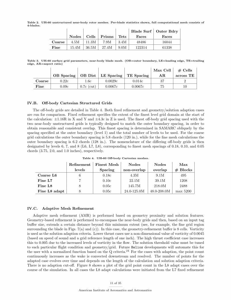
Table 2. UH-60 unstructured near-body rotor meshes. Per-blade statistics shown, full computational mesh consists of4-blades.

Blade Surf Outer BdryNodes Cells Prisms Tets Faces Faces

Coarse 4.5M 11.3M 7.9M 3.4M 48486 16044Fine 15.4M 36.5M 27.4M 9.0M 122314 61338

Table 3. UH-60 surface grid parameters, near-body blade mesh. (OB=outer boundary, LE=leading edge, TE=trailingedge, AR=aspect ratio)

Max Cell # CellsOB Spacing OB Dist LE Spacing TE Spacing AR across TE

Coarse 0.22c 1.6c 0.0029c 0.014c 37 2Fine 0.09c 0.7c (cut) 0.0067c 0.0067c 75 10

IV.B. Off-body Cartesian Structured Grids

The off-body grids are detailed in Table 4. Both fixed refinement and geometry/solution adaption casesare run for comparison. Fixed refinement specifies the extent of the finest level grid domain at the start ofthe calculation: ±1.16R in X and Y and ±4.3c in Z is used. The finest off-body grid spacing used with thetwo near-body unstructured grids is typically designed to match the outer boundary spacing, in order toobtain reasonable and consistent overlap. This finest spacing is determined in SAMARC obliquely by thespacing specified at the outer boundary (level 1) and the total number of levels to be used. For the coarsegrid calculations the outer boundary spacing is 5.8 chords (120 in.), while for the fine mesh calculations theouter boundary spacing is 6.2 chords (128 in.). The nomenclature of the differing off-body grids is thendesignated by levels 6, 7, and 8 (L6, L7, L8), corresponding to finest mesh spacings of 0.18, 0.10, and 0.05chords (3.75, 2.0, and 1.0 inches), respectively.

Table 4. UH-60 Off-body Cartesian meshes.

Refinement Finest Mesh Nodes Nodes Maxlevels Spacing non-overlap overlap # Blocks

Coarse L6 6 0.18c 4.3M 9.1M 495Fine L7 7 0.10c 22.1M 39.1M 1208Fine L8 8 0.05c 145.7M 218.0M 2488Fine L8 adapt 8 0.05c 24.0-125.0M 48.0-208.0M max 5200

IV.C. Adaptive Mesh Refinement

Adaptive mesh refinement (AMR) is performed based on geometry proximity and solution features.Geometry-based refinement is performed to encompass the near-body grids and then, based on an input tagbuffer size, extends a certain distance beyond this minimum extent (see, for example, the fine grid regionsurrounding the blade in Figs. 7(a) and (c)). In this case, the geometry-refinement buffer is 8 cells. Vorticityis used as the solution adaption criteria. Lower thrust cases use a non-dimensional value of vorticity of 0.0045(based on speed of sound and a grid reference length of one inch). The high thrust coefficient case increasesthis to 0.005 due to the increased levels of vorticity in the flow. The solution threshold value must be tunedto each particular flight condition and geometry/grid. Future Helios developments will automate this forthe user with a normalized function based on the Q criteria.24 For the cases with adaption, the point countcontinuously increases as the wake is convected downstream and resolved. The number of points for theadapted case evolves over time and depends on the length of the calculation and solution adaption criteria.There is no adaption cut-off. Figure 8 shows a plot of the grid point count in the L8 adapt cases over thecourse of the simulation. In all cases the L8 adapt calculations were initiated from the L7 fixed refinement

11 of 35


solution. Even after 144 adaption cycles (one rotor revolution) the point count is less than that obtainedwith L8 fixed refinement, which is more limited in the extent of wake capture downstream of the rotor.Specifically, the adapted grids for the high speed, low speed, and high thrust coefficient cases have generated67, 59, and 125 million grid points, respectively, after one rotor revolution (only half a rotor revolution forthe high speed case). This is in comparison to the L7 fixed grid with 22 million points, which was used asthe starting point, and the L8 fixed grid with 146 million points.

(a) ψ = 0 deg (b) ψ = 7.5 deg

(c) ψ = 0 deg (d) ψ = 7.5 deg

Figure 7. High speed wake. Vorticity magnitude overlaid on AMR mesh at (a) ψ = 0 deg and (b) ψ = 7.5deg; (c)–(d)close up of third-quadrant tip vortex at these azimuthal locations.

Geometry and solution-based refinement are performed concurrently every 2.5 degs of rotor rotation. Thisis problem dependent, but for conventional rotorcraft the adapt frequency is driven by the rotor rotationspeed and the movement of the rotor tip (advance ratio < 1). Figure 7(a/c) shows an AMR mesh at aparticular time (ψ = 0 deg) and the corresponding vorticity magnitude contours for the high speed case.Also shown are the vorticity contours 7.5 degs later (Figure 7(b/d)) on the same mesh. The maximumvorticity value shown (red) is the refinement criteria (0.0045). It is seen that based on the size of thedefault solution-based buffer region, the high vorticity regions (tip vortices) are just exiting the refinedregion. However, the blade geometry has moved well beyond the fine grid geometry-refinement boundaries,and is, therefore, the limiting factor setting the required frequency of adaption. This could be remedied byincreasing the geometry-based tag buffer region, and would be particularly beneficial for low speed cases inorder to significantly reduce the adaption frequency. However, the cost of an adaption is roughly on theorder of 5 SAMARC steps, or one total Helios step, and is, therefore, relatively efficient given the significant

12 of 35


Figure 8. L8 adaptive grid point count for the three UH-60A flight conditions, compared with L7 and L8 fixedrefinement.

regridding and data communication that is being performed. This amounts to 1% of the total calculationcost.

IV.D. Flow Solver Inputs

The 5th-order ARC3D spatial scheme is employed for off-body calculations. Time integration in the off-body solver uses an explicit time-dependent 3-stage Runge-Kutta scheme which has a CFL limitation on thesize of the timestep for stability. Finer off-body grids require smaller timesteps. For the unsteady coarse gridcalculations with 6 off-body levels, a physical time step of ∆ψ = 0.25 degs is used. This corresponds to anoff-body CFL=1.67, which is slightly high given the target stable CFL is 1.0, but the solution remained stablewith this setting. Enforcing the CFL limitation with finer off-body meshes requires either 1) reducing thephysical timestep ∆ψ, or 2) applying sub-steps within each physical timestep. We chose to use a combinationof these two options. For the medium (7 level) and fine (8 level) off-body grid systems a ∆ψ = 0.1 degs isemployed, and sub-steps are applied to maintain a CFL < 1. Table 5 shows the parameters used. Duringthe off-body substepping, the overset boundary conditions within the off-body solver are updated, however,the near-body overset boundary points cannot be updated due to inconsistent solution methodologies duringsub-stepping/sub-iterating. Since the most significant cost of the Helios solution is the near-body solver, theoff-body substepping provides an efficient alternative to unnecessarily reducing the global time step belowthat required to capture the physics.

Near-body NSU3D calculations use an iterative scheme to converge the solution at each physical timestep. An implicit line solver is applied in the prismatic boundary layer part of the grid, along with multigridacceleration. The number of subiterations are chosen based on the drop in subiteration residual, convergenceof the global rotor forces (CT , CQ) at each time step (Figure 9), and convergence of the section airloadsfrom revolution to revolution. Such convergence criteria typically require at least one order of magnitudereduction in the subiteration residual. Table 5 lists the near-body subiterations and multigrid levels usedfor the UH-60 calculations.

Table 5. Unsteady CFD time-stepping parameters.

Off-body Time step Off-body Near-body Near-bodyLevels (deg Azimuth) Substeps CFL Subiters MG Levels

6 0.25 1 1.67 25 17 0.10 2 0.66 15 38 0.10 3 0.88 15 3

13 of 35


Figure 9. NSU3D fine grid subiteration convergence. left axis: density ρ and force CT , CQ residual increments; rightaxis: normalized CT and CQ convergence (local iteration value divided by final value).

IV.E. CFD/CSD Coupling

For the both the coarse and fine grids fully coupled CFD/CSD results are obtained. For the coarse grid,results are obtained using fixed L6 refinement. On the fine grid, both the low speed transition and highspeed (C8513 and C8534) cases have been fully coupled using L8 adapt. All three cases on the fine gridhave, however, been computed using prescribed motions from coarse grid coupled calculations. The trimconditions (thrust, hub moments, and angle of attack) are taken from the UH-60 Airloads database withcorrections made for fuselage, empennage, and tail rotor lift. The trim conditions are shown in Table 1. Forthe coarse grid coupling is performed every 180 degs of rotor rotation. For the fine grid the frequency isincreased to every 90 degs. All cases are run for at least 6 coupling iterations, which is generally enough forengineering convergence of the coupling procedure.

IV.F. Solution Timing

All cases were run on 256 processors of a Dell PowerEdge M610 (DOD MHPCC mana). Solution timesbroken down by Helios module are shown in Table 6. The near-body (NSU3D) cost is fixed since the near-body grid is unchanged. The off-body solution time varies with the number of grid points. In all cases,the timings are the averaged values for all the flight conditions. Due to the nature of the adaption, thetimings for these cases are approximate. The near-body and off-body timings are generally very repeatablebetween runs. It is seen that the near-body flow solver dominates the cost of the solution, even for the L8grid which has 9.5 times as many off-body as near-body points, making the off-body solver almost 40 timesmore efficient on this grid. It should be noted, however, that the off-body scheme is structured, inviscid andexplicit, while the near-body is unstructured, viscous and implicit. The domain connectivity cost is quitevariable (min/max times are quoted), particularly with finer off-body grids. At best, PUNDIT requires only7% of the time step, although at worst the cost is upwards of 40%. At present we are unclear of the cause.but we have found disk access speeds on the mana system are highly variable and can at times be veryslow. Although communication in the domain connectivity software are not file based, the inter-processor

14 of 35


communication takes place in core memory using MPI, information is written to a centralized log file andthe consequent disk access may be introducing the variability in timing. The issue is under investigation.The total times quoted in the table are based on minimum domain connectivity times. It is seen that onaverage the cost of an adapted solution is on par with a fixed refinement case, with the extra cost due notto adaption but domain connectivity.

Table 6. Breakdown of time per timestep in the CFD solution (seconds/percentage), computed on 256 cores of a DellPowerEdge M610 system.

Adaption Domain ConnNear-body Off-body Overhead (min/max) Total

Coarse L6 13.1 (82%) 0.31 (1%) – 1.28 (7%) 15.8Fine L7 27.5 (86%) 1.3 (4%) – 2.2/5.3 (7%) 31.8Fine L8 27.8 (71%) 6.8 (17%) – 3.7/14.8 (10%) 38.9

Fine L8 adapt 27.0 (54%) 4.0 (17%) 0.8 (2%) 8.9/21.3 (18%) 50.0

V. Results and Discussions

The results are organized as follows. We first present the convergence of the fluid/structure simulationstrategy. Following that more detailed comparisons of sectional aerodynamic loading (both time historyas well as harmonics) with flight test data are demonstrated to verify the prediction capability of Helios.Finally, we illustrate comparisons of wake visualizations with and without solution-based AMR.

V.A. Convergence of Fluid/Structure coupling

Fluid/structure coupling involves exchange of loads/displacements according to a prescribed scheduleuntil convergence of the aerodynamic/structural dynamic loading is attained based on the periodicity of therotor. In Fig. V.A we compare the evolution of steady sectional aerodynamic normal force variation over thespan of the rotor blade with coupling iteration. It can be noticed that the aerodynamic loading approachesthe flight data with coupling iterations and finally shows fair correlation with the measured flight data.Aerodynamic loading (normal force) history at a radial location close to the tip of the blade (96.5% span)is also shown in Fig. V.A. The high speed forward flight condition shows the best convergence and requiresonly six coupling iterations for the variations to be within plotting accuracy. The low speed and stall casesrequire further iterations for tight convergence – though the general pattern of vibratory and oscillatoryairloads are already in place.

V.B. Airload Comparisons

Airloads comparisons are made in this section between the CFD/CSD coupled coarse near-body/L6 off-body and fine near-body/L8 adaptive grid systems. As described previously, prescribed motion cases werealso run for all the flight conditions using L7 fixed refinement, L8 fixed refinement, and L8 adaptive with thefine near-body grid. The differing wake resolutions had minor impact on section airloads and global forcesand moments (rotor thrust and torque). As would be expected, torque was most noticeably dependent onnear-body grid resolution.

V.B.1. High speed forward flight condition (C8534)

The high speed forward flight condition is characterized by high vibratory loads owing to returningwake interactions on the advancing side. Results for this case shown in Fig. 11 indicate good predictionof the advancing blade interaction compared to other state-of-the-art computations.7 Note the lift andpitching moment impulses around 90 degs blade azimuth, indicating resolution of some probable wake-induced vibratory loads on the advancing side. This phenomena is a key contributor to the vibratory liftphase and 3/rev flap bending moment.

The results for the L6 and L8 adaptive grids, which differ significantly in both near-body and off-bodygrid resolution, are quite similar in their ability to capture the salient features of the aerodynamic loading

15 of 35


0 90 180 270 360−600

−300

0

300Normal force at 96.5% R, lb/ft

Flt

853

4

0 0.25 0.5 0.75 10

100

200

300

400Steady normal force, lb/ft

0 90 180 270 360−200

0

200

Flt

851

3

0 0.25 0.5 0.75 10

100

200

300

400

0 90 180 270 360−200

0

200

Azimuth, degs.

Flt

901

7

0 0.25 0.5 0.75 10

100

200

300

400

Radial station r/R

FlightIter 0

Iter 6

Figure 10. Convergence of oscillatory (mean removed) and mean normal forces.

waveform. It appears the L8 adapt grids do show more vibratory characteristics, likely owing to betterresolution of the wake, but the difference is slight. Other studies? have indicated that improved resolutionof both the near- and off-body grids is required for optimal load prediction.

From basic rotor dynamics it is possible to infer that the first two harmonics (of the rotor rotatingfrequency) of the sectional aerodynamic loading do not contribute to fixed frame vibration, if the numberof blades in the rotor is greater than or equal to four. Therefore it is a common practice in the rotary wingcommunity to characterize the vibratory load prediction by plotting sectional aerodynamic loading afterfiltering the first two harmonics of variation. The vibratory part of the aerodynamic loading (3/rev andhigher) for the UH-60A high speed forward flight condition is shown in Fig. 12. The overall waveform ofthe vibratory loading is captured quite well by both mesh systems. Minor improvement in the magnitudeof vibratory lift can be noticed from the adaptive solution (denoted by L8a in plots). It is worth notingthat although the magnitude of vibratory lift from Helios does show improvement from state-of-the-artpredictions, it still remains underpredicted compared to the flight test data.

Basic rotor dynamics also indicates that Nb − 1, Nb and Nb + 1 (Nb=number of blades) harmonics ofrotor frequency in rotating frame loading are the primary contributors to fixed frame vibration. Therefore,for the four-bladed UH-60A rotor, we show the variation of the magnitudes of the 3, 4 and 5/rev rotating

16 of 35


−1

0

1

2

3

Chord Force (lb/in)(mean removed)

22.5

% R

−2

0

2

4

55 %

R

−4

−2

0

2

4

77.5

% R

−4

−2

0

2

4

86.5

% R

0 90 180 270 360−4

−2

0

2

4

Azimuth (deg)

96.5

% R

−10

0

10

20

30

Normal Force (lb/in)

0

10

20

30

40

−20

0

20

40

−50

0

50

0 90 180 270 360−40

−20

0

20

40

Azimuth (deg)

−50

0

50

100

Pitching Moment(lb−in/in)(mean removed)

−40

−20

0

20

−60

−40

−20

0

20

−100

−50

0

50

0 90 180 270 360−100

−50

0

50

Azimuth (deg)

DataHELIOS (L6)HELIOS (L8a)

Figure 11. High speed (C8534) airloads. Predicted and measured airloads for high speed flight using coarse (off-bodyL6) and fine (off-body L8 adapt) grid systems; µ = 0.368; CT /σ = 0.084

17 of 35


−1

0

1

2

Chord Force (lb/in)

22.5

% R

−2

−1

0

1

2

55 %

R

−1

0

1

2

77.5

% R

−1

0

1

2

86.5

% R

0 90 180 270 360−1

−0.5

0

0.5

1

Azimuth (deg)

96.5

% R

−10

−5

0

5

10


−10

−5

0

5

10

−20

−10

0

10

20

−20

−10

0

10

20

0 90 180 270 360−20

−10

0

10

20

Azimuth (deg)

Data

HELIOS (L6)

HELIOS (L8a)

Figure 12. High speed (C8534) vibratory airloads. Predicted and measured vibratory airload (3/rev and higher)time-histories for high speed flight using coarse (off-body L6) and fine (off-body L8 adapt) grid systems; µ = 0.368;CT /σ = 0.084

18 of 35


frame aerodynamic loading with non-dimensional spanwise coordinate in Figure 13. It can be noticed thatadaptive mesh refinement (denoted by L8a in plots) does produce non-negligible improvement in the 3/revand 4/rev harmonics of loading in mid-span locations. Indeed, mid-span locations are where returningwake interactions are prominent at this flight condition, and adaptive mesh refinement contributes to theimprovement of aerodynamic loading at these locations by better capturing the vortex wake field.

V.B.2. Low speed transition flight condition (C8513)

The low speed transition flight condition is also a high vibration flight condition similar to the highspeed flight. The mechanism of vibration is, however, quite different. The aerodynamic loading in this flightcondition is dominated by the interactions of the rotor blade with the rolled up vortex structures on the rearof the rotor disk (often termed ’disk-vortices’ or ’super vortices’). Helios predictions for this flight conditionis shown in Figure 14. The data shows good correlation with the flight test data indicating effective captureof the vortex wake structures. Similar to the high-speed C8534 case, the L6 and L8 adapt grid systems showlargely similar characteristics, although the L8 adapt results do show more vibratory characteristics likelyfrom better resolution of the wake.

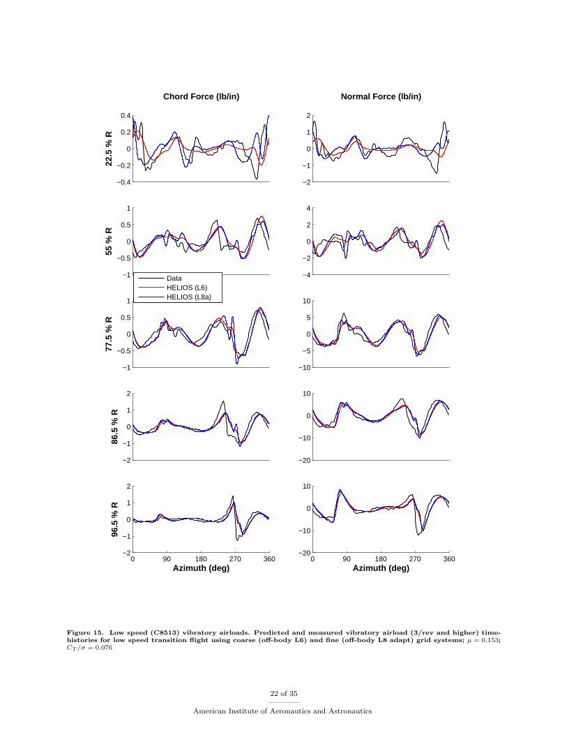
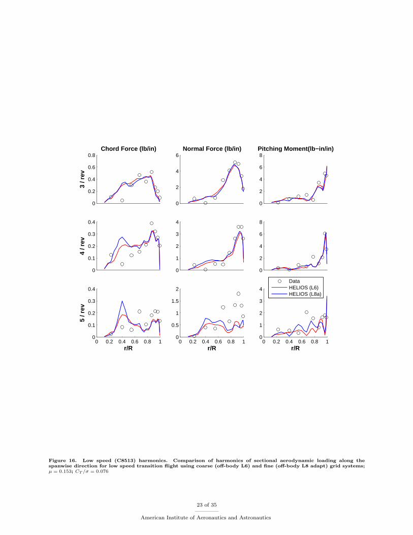
Figure 15 shows the vibratory aerodynamic loading (3/rev and higher) at this flight condition. Thewaveforms of the vibratory loads are in good agreement with flight data for both normal and chord forces.The peak magnitude remains underpredicted, although to a lesser extent compared to high speed forwardflight condition. The variation on rotor frequency harmonics with spanwise coordinate is compared with testdata in Fig. 16. Differences are observed between the L6 and L8 adapt grids but, in general, it is difficultto discern whether the finer L8 adapt off-body grids are leading to improvements in the spanwise harmonicloading as well.

V.B.3. High-altitude stall flight condition (C9017)

The high altitude stall flight condition represents one of the extremes in the level flight operating envelope.The high thrust generated at this condition causes distinct dynamic stall events on the retreating blade.These stall events dominate the high frequency blade pitch excitation causing large torsion moments andconsequently large push-rod loads (almost the maximum in level flight).

For this flight condition, the target thrust was arbitrarily reduced by 5% from the previously publishedCT /σ = 0.129 to CT /σ = 0.126 due to well known uncertainties associated with this flight. Unlike the othertwo flight conditions, this flight occurs at the stall boundary of the rotor, and achieving the correct trimstate is a critical pre-requisite to any meaningful stall prediction.

The retreating blade stall events in the aerodynamic loading is the key phenomena that needs to beresolved at this flight condition. From Fig. 17 it is evident that the two stall cycles are resolved quiteaccurately at the stations outboard of 80%. The advancing blade lift waveform, however, is not as wellpredicted as the other two flight conditions. This is partly due to previously described differences in thetrim targets. Coupled solutions were available only using the coarse grid (L6) at the time of preparationof this article. We compare the coarse grid solutions with an adaptive solution obtained by prescribing theblade motions obtained from the coarse grid coupled solution (represented as L8a-prescribed) in the figure.We observe noticeable improvements in prediction of stall patterns (especially in the inboard stations) whenAMR is utilized. This improvement is also evident in the harmonic variation with span coordinate (shown inFig. 18), where the AMR clearly shows improved magnitude of the vibratory airloads. Torsion moments andpush-rod loads at this flight conditions are characterized by the presence of large 5/rev magnitude harmonicsowing to the frequency content of the two prominent stall cycles in the pitching moment wave form. It isworth noting that the 5/rev harmonic variation across span is well captured by both grid systems, with theAMR grid system showing comparatively better prediction inboard.

V.C. Wake Comparisons

Figure 19 show a top view comparison of the wakes for the various grid combinations – L6, L7, L8, andL8 adapt – for the high speed (C8534) case. For the fixed refinement calculations ((a)–(c)) the wake detailis increasingly well captured as indicated by the iso-surface of the Q criteria (Q ∗R2 = 0.3). The grid showsthe extent of the fixed refinement region. For the L8 off-body grids ((c)–(d)) only every other point is shown.The adapted grid (d) maintains clustering near the tip and root vortices and vortices emanating from the

19 of 35


0

0.2

0.4

0.6

0.8Chord Force (lb/in)

3 / r

ev

0

0.2

0.4

0.6

0.8

4 / r

ev

0 0.2 0.4 0.6 0.8 10

0.2

0.4

0.6

0.8

r/R

5 / r

ev

0

2

4

6

8Normal Force (lb/in)

0

2

4

6

0 0.2 0.4 0.6 0.8 10

1

2

3

r/R

0

10

20

30Pitching Moment(lb−in/in)

0

5

10

15

0 0.2 0.4 0.6 0.8 10

2

4

6

r/R


Figure 13. High speed (C8534) harmonics. Comparison of harmonics of sectional aerodynamic loading along thespanwise direction for high speed flight using coarse (off-body L6) and fine (off-body L8 adapt) grid stem’s; µ = 0.368;CT /σ = 0.084

20 of 35


−0.5

0

0.5

1


22.5

% R

−2

−1

0

1

2

55 %

R

−1

0

1

2

77.5

% R

−1

0

1

2

86.5

% R

0 90 180 270 360−1

0

1

2

Azimuth (deg)

96.5

% R

0

5

10

15


10

15

20

25

30

15

20

25

30

35

10

20

30

40

0 90 180 270 3600

10

20

30

40

Azimuth (deg)

−5

0

5

10


−20

−10

0

10

−10

−5

0

5

10

−20

−10

0

10

20

0 90 180 270 360−40

−20

0

20

40

Azimuth (deg)

Data

HELIOS (L6)

HELIOS (L8a)

Figure 14. Low speed (C8513) airloads. Predicted and measured airloads for low speed transition flight using coarse(off-body L6) and fine (off-body L8 adapt) grid systems; µ = 0.153;CT /σ = 0.076

21 of 35


−0.4

−0.2

0

0.2

0.4

Chord Force (lb/in)22

.5 %

R

−1

−0.5

0

0.5

1

55 %

R

−1

−0.5

0

0.5

1

77.5

% R

−2

−1

0

1

2

86.5

% R

0 90 180 270 360−2

−1

0

1

2

Azimuth (deg)

96.5

% R

−2

−1

0

1

2


−4

−2

0

2

4

−10

−5

0

5

10

−20

−10

0

10

0 90 180 270 360−20

−10

0

10

Azimuth (deg)


Figure 15. Low speed (C8513) vibratory airloads. Predicted and measured vibratory airload (3/rev and higher) time-histories for low speed transition flight using coarse (off-body L6) and fine (off-body L8 adapt) grid systems; µ = 0.153;CT /σ = 0.076

22 of 35


0

0.2

0.4

0.6


3 / r

ev

0

0.1

0.2

0.3

0.4

4 / r

ev

0 0.2 0.4 0.6 0.8 10

0.1

0.2

0.3

0.4

r/R

5 / r

ev

0

2

4


0

1

2

3

4

0 0.2 0.4 0.6 0.8 10

0.5

1

1.5

2

r/R

0

2

4

6


0

2

4

6

8

0 0.2 0.4 0.6 0.8 10

1

2

3

4

r/R


Figure 16. Low speed (C8513) harmonics. Comparison of harmonics of sectional aerodynamic loading along thespanwise direction for low speed transition flight using coarse (off-body L6) and fine (off-body L8 adapt) grid systems;µ = 0.153; CT /σ = 0.076

23 of 35


swept tip break. The wake sheet in the 2nd quadrant is also picked up by the adaption. Comparing theL8 fixed refinement and adapted cases indicates very little difference in the structure. The most noticeabledifference is in the 4th quadrant. The adapted grid does a much better job at resolving the region outsideof the fixed refinement box. For clarity the near-body grids have not been shown, although the hole cuts inthe off-body meshes indicate their appropriate location.

Figure 20 shows a comparison of the vorticity contours in a streamwise cut at 62% span on the retreatingside for the high speed (C8534) case. The maximum vorticity shown is the refinement criteria (0.0045 non-dimensional). Again the wake is increasingly well captured as the off-body grid is refined ((a)-(c)). Thecut off and dissipation of the vortex at the downstream boundary of the refinement region is drastic. Forthis flight condition the refined region is poorly placed and should be moved downward, but this is flightcondition dependent. The adapted solution (d) removes the requirement to know the location of the wakea priori. It does an excellent job of capturing the tip vortices with the finest refinement level. The vorticesare effectively tracked continuously downstream. Unlike the L8 fixed refinement case (c) the shear layers arenot fully refined so that the vorticity contours differ visually. The location of the blade is indicated by theblanked out region and is seen to have geometry adaption (Fig. 20(d)).

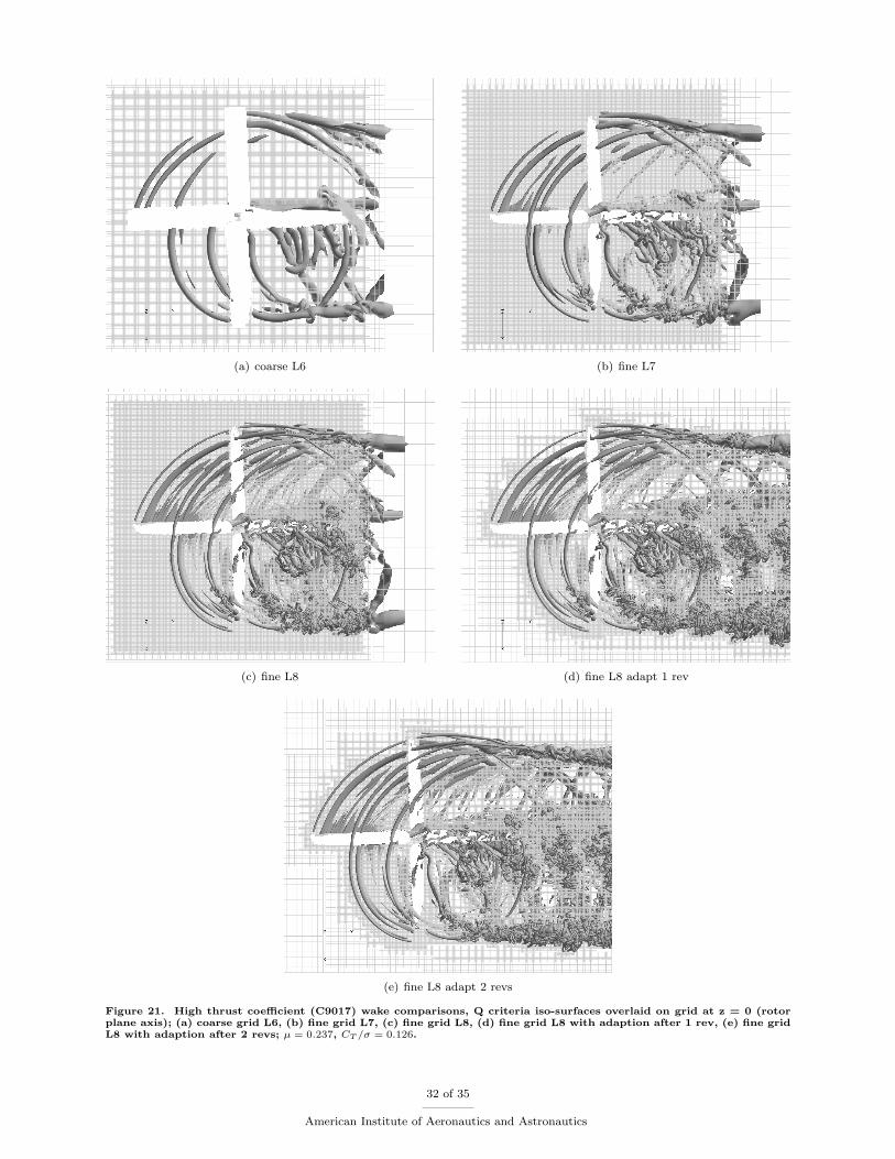
At the start of the adaption calculation the L8 adapted grid has only 29 million grid points used to refineto the geometry and solution in the fixed refinement region. This is a significant savings over the L8 fixedrefinement box which required 146 million points and is comparable to the 22 million required for the L7fixed refinement case but with better resolution. At the end of the adaption portion of the calculation, i.e.half a rotor revolution for C8534, the L8 adapted grid (Fig. 20(d)) has half the number of grid points as theL8 fixed grid (Fig. 20(c)) – 67 million compared with 146 million. Overall, there is a much more efficient useof grid points (computational resources) with the adaption scheme throughout the calculation.

Figures 21 and 22 shown Q iso-surfaces (top view) and vorticity contours (side view, retreating side, 62%span) for the high thrust coefficient case (C9017). The top view (Figure 21) clearly shows the wake and shedvorticity being increasingly well captured with increasing grid density. The L8 grids (fixed and adapted)capture the same wake structures (Fig. 21(c-d)). This includes what appears to be a ”bursting” of the tipvortex early in the 4th quadrant and the entrainment of this structure into the retreating-side super-vortex.A significant amount of turbulent wake is also generated from the hub vortices and their interaction withthe stall cycle late in the 4th quadrant. This detailed type of turbulent (i.e. chaotic) wake structure has notbeen seen previously in UH-60 high thrust coefficient calculations and deserves further investigation as tothe causes and effects of these instabilities.

In the vorticity contours (Fig. 22) it is seen that the L8 fixed refinement actually better captures someof the wake sheets and maintains the older vortices longer compared with the L8 adapted grid after 1 rotorrevolution (Fig. 22(d)). The older vortices (from the front of the rotor disk) are lower in the side view.The vorticity magnitude of these older structures that originated in the non-refined L7 fixed grid startingsolution were not strong enough to be identified by the feature-based refinement procedure. In this sense, thefixed L8 refinement would seem to be better capturing the wake, and the reduction in vorticity of the oldervortices would appear to be an artifact of the adaption. However, additional visualization of the adaptedsolution after 2 rotor revolutions (Fig. 22(e)) indicates that vortices which originate in the L8 refined meshare properly maintained. This delay in adapting to the vortex is due to 1) the choice of adaption criteria (i.e.vorticity) and 2) the physical time it takes for the highly resolved adaption regions to be ”convected” withthe flow. This second point is a function of the starting conditions for the AMR calculations (L7 fixed in thiscase). Additional study of the effects of time-dependent AMR on rotorcraft flowfields, including adaptionfrequency, extent of buffer regions, and grid interpolation on vortex capturing is required to understand thisphenomenon. Note that the Cartesian ”holes” in the L8 off-body grid that are not associated with the bladehole cuts (e.g. regions between refinement levels) are an artifact of plotting every other point.

Due to a combination of lower advance ratio producing more wake, increased thrust producing highervorticity levels, and shed vorticity from the stall regions, this case generates the most grid points from solutionadaption. The vorticity adaption criteria was only increased slightly from 0.0045 to 0.0050 to account for theincreased levels of vorticity. At the adaption initiation from L7 fixed, 36 million grid points are generated.The adaption portion of the calculation results in 125 million grid points after one rotor revolution, andover 240 million points after 2.5 rotor revolutions. For one rotor revolution, the L8 adapt point count is,therefore, still less than the L8 fixed refinement (145 million) case but with noticeable differences in wakecapturing as previously described. The cost of refinement and the associated domain connectivity make thiscalculation approximately 12% more expensive on average.

24 of 35


Finally, for completeness, Figs. 23 and 24 shown Q iso-surfaces and vorticity contours for the low speedcase (C8513). The trends from the previous cases are maintained. Even though the advance ratio is low,which maintains more revolutions of the wake near the plane of the rotor, (compare Figs. 19 and 23), theL8 adaption grid point count is not as large as would be expected. In fact, the starting and ending pointcount values (after one rotor revolution) of 24 and 59 million are the lowest of the three flight conditions. Inthis case the L8 adapt cost is 12% less than the fixed refinement. However, as in the high thrust coefficientcase, the wake sheets and older wake ages are not always well captured or maintained (Fig. 24(d)) unlessadditional rotor revolutions are performed (Fig. 24(e)).

VI. Concluding Observations

This article describes the CFD/CSD implementation of the Helios software framework and validates itsprediction capability using experimental flight data from the UH-60 rotorcraft in three flight conditions. Thecomputations exercise all of the capabilities of Helios including adaptive mesh refinement, automated over-set domain connectivity and seamless in-core fluid/structure coupling. Furthermore, this is perhaps the firstsuccessful demonstration of solution based adaptive mesh refinement for the complex coupled fluid/structureproblem encountered in rotorcraft aeromechanics, particularly in forward flight. Key observations and con-clusions are summarized below.

1. The CFD flow solution process involving a dual-mesh paradigm – unstructured near-body solver(NSU3D), Cartesian-adaptive off-body solver (SAMARC), and automated parallel domain connec-tivity (PUNDIT) – is verified to be robust for application in rotary-wing systems with relative motionand elasticity.

2. Some outstanding issues were identified with respect to solution timings. In particular, the cost ofdomain connectivity was quite variable, sometimes as low as 7% while at other times as high as 40%of the total cost per step, with some dependency on AMR (i.e. grid point and grid block count). Also,the cost of the unstructured near-body solution at each unsteady timestep remains high relative tocalculations with structured-grid solvers.

3. The fluid/structure interface process used by Helios is verified to be seamless, consistent, and accurate,hence providing accurate and convergent solutions to the coupled fluid/structure/vehicle trim problem.

4. The off-body AMR scheme generally achieves equal accuracy in the wake as compared to a finely-resolved fixed refinement off-body grid with equal resolution but with significantly fewer gridpoints.It also aids in automatically preserving flow features for much larger distances/times downstream ofthe rotor, which removes from the user the burden of having to define, a priori, the condition/problemdependent wake location. In certain cases, older vortices from the front of the rotor disk were not alwayswell captured by vorticity-based adaption, thus motivating the development of more sophisticatedfeature detection criteria and schemes.

5. The improved wake resolution with AMR is found to have minimal impact on aerodynamic sectionalloading predictions (normal force, chord force, and pitching moment). Furthermore, global force pre-diction (thrust and torque coefficient) showed little sensitivity to off-body wake resolution, basedon prescribed motion calculations with various levels of off-body spacing using fixed refinement andfeature-based adaption. This suggests that the fine wake resolution from AMR is not absolutelyrequired for obtaining reasonable aerodynamic loading predictions for the three level forward flightconditions studied. This would not be a likely conclusion for blade-vortex interaction (BVI) analysis.

6. Although the AMR scheme reduces the off-body grid point count, the cost of solutions are not signifi-cantly changed compared with equivalently fine fixed refinement meshes (±12%). One reason is thatAMR maintains the wake for much larger downstream distances and, in some cases, creates compara-ble amounts of grid points as a case with fixed refinement. This effect can be mitigated by limitingthe extent of the wake tracking and adaption, although maintaining refinement of the wake may bepreferable for modeling rotor/fuselage or main-rotor/tail-rotor interactions. Another is that AMR in-troduces many more grid blocks which potentially increases domain connectivity cost. Nonetheless,the off-body solution component is quite fast compared with the near-body module, on average about

25 of 35


15% of the total cost. Even significant efficiency improvements to the off-body solution will thus havea lesser impact on the overall cost.

7. Further study of the effects of AMR on a range of rotorcraft flowfields (i.e. BVI and hover), performanceprediction, and wake capturing is required. This includes automation of the feature detection andoptimization of the adaption parameters, such as extent and frequency.

VII. Acknowledgments

Material presented in this paper is a product of the CREATE-AV (Air Vehicles) Element of the Compu-tational Research and Engineering for Acquisition Tools and Environments (CREATE) Program sponsoredby the U.S. Department of Defense HPC Modernization Program Office. This work was conducted at theHigh Performance Computing Institute for Advanced Rotorcraft Modeling and Simulation (HIARMS). Theauthors gratefully acknowledge additional contributions by Dr. Venkateswaran Sankaran, Dr. Roger Strawn,and Prof. Dimitri Mavriplis. The authors gratefully acknowledge the use of the DoD High PerformanceComputing and Modernization Office (HPCMO) DOD Shared Resource Centers (DSRC).

References

1Sankaran, V., J. Sitaraman, A. Wissink, A. Datta, B. Jayaraman, M. Potsdam D. Mavriplis, Z. Yang, D. O’Brien,H. Saberi, R. Cheng, N. Hariharan, and R. Strawn, “Application of the Helios Computational Platform to Rotorcraft Flowfields,”AIAA-2010-1230, 48th AIAA Aerospace Sciences Meeting, Orlando FL, Jan 2010.

2J. Sitaraman, A. Katz, B. Jayaraman, A. Wissink, V. Sankaran, “Evaluation of a multi-solver paradigm for CFD usingoverset unstructured and structured adaptive Cartesian grids,” AIAA-2008-0660, AIAA 48th Aerospace Sciences Meeting, RenoNV, Jan. 2008.

3J. Sitaraman, M. Floros, A. Wissink, M. Potsdam,”Parallel Domain Connectivity Algorithm For Unsteady Flow Com-putations Using Overlapping And Adaptive Grids,” Journal of Computational Physics, Volume 229, Issue 12, p. 4703-4723.

4A. Wissink, S. Kamkar, T. Pulliam, J. Sitaraman, and V. Sankaran, “Cartesian Adaptive Mesh Refinement for RotorcraftWake Resolution,” AIAA-2010-4554, AIAA 28th Applied Aerodynamics Conference, Chicago IL, June 2010.

5S. Choi, and A. Datta, “CFD Prediction of Main Rotor Vibratory Loads Using Time-Spectral Method,” AIAA Paper2008-7325, 26th AIAA Applied Aerodynamics Conference, Honolulu, Hawaii, Aug. 18-21, 2008.

6A. Wissink, J. Sitaraman, D. Mavriplis, T. Pulliam, V. Sankaran, “A python-based infrastructure for overset CFD withadaptive Cartesian grids,” AIAA-2008-0927, AIAA 48th Aerospace Sciences Meeting, Reno NV, Jan. 2008.

7M. Potsdam, H. Yeo, and W. Johnson, “Rotor Airloads Prediction Using Loose Aerodynamic/Structural DynamicCoupling,” Presented at the 60th Forum of American Helicopter Society, Baltimore, MD, May 2004.

8Wissink, A.M., M. Potsdam, V. Sankaran, J. Sitaraman, Z. Yang, and D. Mavriplis, “A Coupled Unstructured-AdaptiveCartesian CFD Approach for Hover Prediction,” Presented at the 66th Forum of the American Helicopter Society, Phoenix AZ,May 11-16, 2010.

9J. Sitaraman, J. D. Baeder, “Evaluation of the wake prediction methodologies used in CFD based rotor airload compu-tations,” AIAA-2006-3472, AIAA 24th Conference on Applied Aerodynamics, Washington, DC, 2006.

10R. Biedron and E. Lee-Rausch, “Rotor Airloads Prediction Using Unstructured Meshes and Loose CFD/CSD Coupling”,Paper AIAA-2008-7341, 26th AIAA Applied Aerodynamics Conference, Honolulu, Hawaii, Aug. 18-21, 2008.

11Z. Yang, D. Mavriplis, “Higher-order time integration schemes for aeroelastic applications on unstructured meshes,”AIAA-2006-0441, AIAA 44th Aerospace Sciences Meeting, Reno NV, Jan. 2006.

12R. D. Hornung, A. M. Wissink, S. R. Kohn, “Managing complex data and geometry in parallel structured AMRapplications,” Engineering with Computers, Vol. 22, No. 3, 2006, pp. 181–195.

13Saberi, H., Khoshlahjeh, M., Ormiston, R., and Rutkowski, M. J., “Overview of RCAS and Application to AdvancedRotorcraft Problems,” 4th AHS Decennial Specialist’s Conference on Aeromechanics, San Francisco, CA, January 21-23, 2004.

14J. J. Alonso, P. LeGresley, E. Van Der Weide, “pyMDO: A framework for high-fidelity multi-disciplinary optimization,”AIAA-2004-4480, AIAA/ISSMO 10th Conference on Multidisciplinary Analysis and Optimization, Washington, DC, 2004.

15M. J. Berger, P. Colella, “Local adaptive mesh refinement for shock hydrodynamics,” Journal of Computational Physics,Vol. 82, No. 1, 1989, pp. 65–84.

16Mavriplis, D. and Levy, W., D., “Transonic Drag Prediction Using an Unstructured Multigrid Solver”, Journal ofAircraft, Vol. 42, No. 4, July-August, 2005.

17Mavriplis, D., “DLRF6 WB and WBF Results using NSU3D,” Proceedings of the 3rd Drag Prediction Workshop, SanFrancisco, CA, June 2006.

18Pulliam, T. H., “Euler and Thin-Layer Navier-Stokes Codes: ARC2D, and ARC3D,” Computational Fluid DynamicsUsers Workshop, The University of Tennessee Space Institute, Tullahoma, Tennessee, March 12-16, 1984.

19Y. Lee, J. D. Baeder, “Implicit hole cutting - a new approach to overset grid connectivity,” AIAA-2003-4128, AIAA16th Conference on Computational Fluid Dynamics, Washington, DC, 2003.

20R. L. Meakin, A. M. Wissink, W. C. Chan, S. A. Pandya, J. Sitaraman, “On strand grids for complex flows,” AIAA-2007-3834, AIAA 18th Conference on Computational Fluid Dynamics, Miami FL, June 2007.

21W. G. Bousman and R. M. Kufeld, “UH-60A Airloads Catalog,” NASA TM-2005-212827/AFDD TR-05-003, 2005.

26 of 35


22R. M. Kufeld, D. L. Balough, J. L. Cross, K. F. Studebaker, C. D. Jennison, and W. G. Bousman, “Flight Testing ofthe UH-60A Airloads Aircraft,” Presented at the 50th Forum of the American Helicopter Society, Washington, DC, May 1994.

23C. Tung, F. X. Caradonna, and W. R. Johnson, “The Prediction of Transonic Flows on an Advancing Rotor, Presentedat the 40th Forum of the American Helicopter Society,” Arlington, VA, May 1984.

24Kamkar, S.J., A. Wissink, V. Sankaran, A. Jameson, “Feature-Driven Cartesian Adaptive Mesh Refinement in the HeliosCode,” AIAA-2010-171, 48th AIAA Aerospace Sciences Meeting, Orlando FL, Jan 2010.

27 of 35


−1

−0.5

0

0.5

1


22.5

% R

−2

0

2

4

55 %

R

−4

−2

0

2

4

77.5

% R

−2

0

2

4

86.5

% R

0 90 180 270 360−2

0

2

4

Azimuth (deg)

96.5

% R

−5

0

5

10


0

10

20

30

10

20

30

40

50

0

20

40

60

0 90 180 270 360−20

0

20

40

Azimuth (deg)

−10

0

10

20


−40

−20

0

20

−100

−50

0

50

−100

−50

0

50

0 90 180 270 360−50

0

50

Azimuth (deg)

Data

HELIOS (L6)

HELIOS(L8a−prescribed)

Figure 17. High thrust coefficient (C9017) airloads. Predicted and measured airloads using coarse (off-body L6) andfine (off-body L8 adapt) grid systems; µ = 0.237;CT /σ = 0.126

28 of 35


0

0.5

1


3 / r

ev

0

0.2

0.4

0.6

0.8

4 / r

ev

0 0.2 0.4 0.6 0.8 10

0.2

0.4

0.6

0.8

r/R

5 / r

ev

0

2

4


0

1

2

3

4

0 0.2 0.4 0.6 0.8 10

1

2

3

r/R

0

5

10


0

5

10

15

0 0.2 0.4 0.6 0.8 10

5

10

15

20

r/R

DataHELIOS (L6)HELIOS (L8a prescribed)

Figure 18. High thrust coefficient (C9017) harmonics. Comparison of various harmonics of sectional aerodynamicloading along the spanwise direction using coarse (off-body L6) and fine (off-body L8 adapt) grid systems; µ = 0.237;CT /σ = 0.126

29 of 35


(a) coarse L6 (b) fine L7

(c) fine L8 (d) fine L8 adapt

Figure 19. High speed (C8534) wake comparisons, Q criteria iso-surfaces overlaid on grid at z = 0 (rotor plane axis);(a) coarse grid L6, (b) fine grid L7, (c) fine grid L8, (d) fine grid L8 with adaption, µ = 0.368, CT /σ = 0.084.

30 of 35



(c) fine L8 (d) fine L8 adapt

Figure 20. High speed (C8534) wake comparisons, vorticity contours overlaid on grid at rotor r/R=0.62 spanwiselocation on retreating size (3rd and 4th quadrant); (a) coarse grid L6, (b) fine grid L7, (c) fine grid L8, (d) fine gridL8 with adaption, µ = 0.368, CT /σ = 0.084.

31 of 35



(c) fine L8 (d) fine L8 adapt 1 rev

(e) fine L8 adapt 2 revs

Figure 21. High thrust coefficient (C9017) wake comparisons, Q criteria iso-surfaces overlaid on grid at z = 0 (rotorplane axis); (a) coarse grid L6, (b) fine grid L7, (c) fine grid L8, (d) fine grid L8 with adaption after 1 rev, (e) fine gridL8 with adaption after 2 revs; µ = 0.237, CT /σ = 0.126.

32 of 35





Figure 22. High thrust coefficient (C9017) wake comparisons, vorticity contours overlaid on grid at rotor r/R=0.62spanwise location on retreating size (3rd and 4th quadrant); (a) coarse grid L6, (b) fine grid L7, (c) fine grid L8, (d)fine grid L8 with adaption after 1 rev, (e) fine grid L8 with adaption after 2 revs; µ = 0.237, CT /σ = 0.126.

33 of 35





Figure 23. Low speed (C8513) wake comparisons, Q criteria iso-surfaces overlaid on grid at z = 0 (rotor plane axis);(a) coarse grid L6, (b) fine grid L7, (c) fine grid L8, (d) fine grid L8 with adaption after 1 rev, (e) fine grid L8 withadaption after 2 revs; µ = 0.150, CT /σ = 0.076.

34 of 35





Figure 24. Low speed (C8513) wake comparisons, vorticity contours overlaid on grid at rotor r/R=0.62 spanwiselocation on retreating size (3rd and 4th quadrant); (a) coarse grid L6, (b) fine grid L7, (c) fine grid L8, (d) fine gridL8 with adaption after 1 rev, (e) fine grid L8 with adaption after 2 revs; µ = 0.150, CT /σ = 0.076.

35 of 35


rotor loads prediction using helios: a multi-solver

Documents