NCAT Report 05-07

ROUND ROBIN EVALUATION OF NEW TEST PROCEDURES FOR DETERMINING THE BULK SPECIFIC GRAVITY OF FINE AGGREGATE By Brian D. Prowell Nolan V. Baker

B

November 2005

277 Technology Parkway Auburn, AL 36830

ROUND ROBIN EVALUATION OF NEW TEST PROCEDURES FOR

DETERMINING THE BULK SPECIFIC GRAVITY OF FINE AGGREGATE

By

Brian D. Prowell Assistant Director

National Center for Asphalt Technology Auburn University, Auburn, Alabama

Nolan V. Baker

Engineer Anderson Engineers

Sarasota Beach, Florida (Formerly of National Center for Asphalt Technology)

Sponsored by

Federal Highway Administration and

National Asphalt Pavement Association

NCAT Report 05-07

November 2005

- i -

DISCLAIMER

The contents of this report reflect the views of the authors who are responsible for the facts and accuracy of the data presented herein. The contents do not necessarily reflect the official views or policies of the Federal Highway Administration, National Asphalt Pavement Association, the National Center for Asphalt Technology, or Auburn University. This report does not constitute a standard, specification, or regulation.

- ii -

TABLE OF CONTENTS Introduction................................................................................................................1 Purpose and Scope .....................................................................................................2 Materials ............................................................................................................2 Proposed Methods......................................................................................................3 InstroTek Corelok ..........................................................................................3 Thermolyne SSDetect ....................................................................................5 Ruggedness Testing ...................................................................................................6 InstroTek Ruggedness Results.......................................................................7 Percent Absorption.............................................................................8 Bulk Specific Gravity ........................................................................10 Apparent Specific Gravity .................................................................12 Additional Investigation of Significant Factors for InstroTek Procedure ...........................................................................................12 Thermolyne SSDetect Ruggedness Results ...................................................16 Percent Absorption and Bulk Specific Gravity..................................16 Apparent Specific Gravity .................................................................18 Round Robin Testing .................................................................................................20 Comparison of Bias between Automated Methods and AASHTO T 84 Results ............................................................................................................20 Water Absorption...............................................................................21 Apparent Specific Gravity .................................................................22 Bulk Dry Specific Gravity ................................................................23 Precision of Test Methods .............................................................................24 AASHTO T 84...................................................................................24 Corelok Method .................................................................................28 SSDetect.............................................................................................32 Comparison of Precision of AASHTO T 84 and New Methods .......36 Recommended Precision Statements .................................................39 Conclusions ............................................................................................................40 Recommendations......................................................................................................42 Acknowledgements....................................................................................................43 Glossary .....................................................................................................................43 References..................................................................................................................45 Appendix A - Ruggedness Study...............................................................................46 Appendix B - Corelok Test Method in AASHTO Format.........................................50 Appendix C – SSDetect Test Method in AASHTO Format ......................................62 Appendix D – Round Robin Results..........................................................................71

- iii -

ABSTRACT This study evaluated two automated methods for determining the dry bulk specific gravity (Gsb) of fine aggregates, the Thermolyne SSDetect and InstroTek Corelok. Each proposed method was evaluated against the standard method described in AASHTO T 84. The evaluation was based on a round robin study with twelve labs and six materials, four crushed fine and two uncrushed (natural) fine aggregate sources. The Corelok and SSDetect methods of determining fine aggregate specific gravity offer significant timesavings over AASHTO T 84. Both the Corelok and SSDetect methods generally produce Gsb results that are similar to AASHTO T 84. It is believed that AASHTO T 84 may not produce accurate results for angular materials with high dust contents. More frequent statistical differences exist between both the Corelok and SSDetect apparent specific gravity (Gsa) and water absorption results and the AASHTO T 84 results than were observed for Gsb. However, Gsa and water absorption are not used in volumetric calculations for hot mix asphalt. Both new methods offer improved precision as compared to AASHTO T 84, particularly for crushed materials with high dust contents.

Prowell & Baker

1 1

ROUND ROBIN EVALUATION OF NEW TEST PROCEDURES FOR DETERMINING THE BULK SPECIFIC GRAVITY OF FINE AGGREGATE

Brian D. Prowell and Nolan V. Baker

INTRODUCTION Determining the bulk specific gravity of fine aggregate is very important when designing a hot mix asphalt (HMA) pavement and for other uses. The bulk specific gravity is used in calculating the voids in the mineral aggregate (VMA) of an HMA mixture. The current methods of determining dry bulk specific gravity (Gsb) of fine aggregates, AASHTO T 84 (1) or ASTM C 128 (2), use a cone and tamp to determine the saturated surface-dry (SSD) condition of a fine aggregate. This method does not work well when determining the SSD condition of angular or rough fine aggregates because they do not readily slump. Therefore, a more accurate and more repeatable method of determining Gsb is needed to provide lower variability between operators and to address problems with angular materials. In order to solve this problem, a method that is more automated and less user dependent is needed to determine both Gsb and absorption of fine aggregates. The Gsb of an aggregate is defined as the ratio of the mass of dry aggregate to the mass of water having a volume equal to that of the aggregate including both its permeable and impermeable voids. Permeable voids are those voids that are filled with water when in the SSD condition and impermeable voids are the voids that water cannot penetrate. Gsb is defined by Equation 1.

Gsb = (Ws / (Vs + Vv))/ γw (1) Ws = mass of solid Vs = Volume of solid (including volume of impermeable voids) Vv = Volume of water permeable voids

γw = Density of water (at a stated temperature) The apparent specific gravity (Gsa) is defined as the ratio of the weight of dry aggregate to the weight of water having a volume equal to the solid volume of the aggregate excluding its permeable voids. Gsa is defined by Equation 2.

Gsa = (Ws / Vs) / γw (2)

An aggregate is said to be in the SSD condition when the permeable voids in the aggregate are filled with water, but outside (surface) moisture is not present on the particle. To reach this SSD condition, the current method (AASHTO T 84) calls for an aggregate to be immersed in water for 15–19 hours and then dried back to this “SSD” state (1). During the 1970s, The Arizona Department of Transportation (DOT) developed a prototype for determining SSD using a rotating vertical tube. Warm air was blown through the tube while it rotated. Using the plots of the inlet and outlet temperature and the basic principles of thermodynamics, they determined the SSD region of these plots. The prototype gave

Prowell & Baker

2 2

encouraging results; however, it had a high variability. The researchers recommended testing a wider variety of fine aggregates (3). NCAT continued with Arizona DOT’s ideas. Instead of blowing warm air vertically over the sample, NCAT tried blowing the warm air longitudinally in a steel drum while it was rotating on its side. NCAT discovered that the SSD point could be determined on a more repeatable basis by monitoring the outgoing relative humidity. There were several problems with this method though: inconsistent drying, loss of fines, clogging of screens, aggregate sticking to the drum and the prototype was not automated (4). Haddock and Prowell (5) explored how InstroTek’s prototype and Thermolyne’s SSDetect determined Gsb. Bulk specific gravities for InstroTek’s prototype were determined from the apparent specific gravities measured with the device assuming constant water absorption for each aggregate type (absorption values were determined at the beginning of a project with ASTM C 128). It was concluded that both prototypes improved the precision of Gsb measurements over the standard method. Hall (6) compared InstroTek prototype’s variability to that of the standard method (AASHTO T 84) using six Arkansas aggregates. Hall concluded that from a practical standpoint, the Gsb and absorption values for both methods were comparable in most cases. However, statistically significant differences existed between the absorption and Gsb measured in three of six cases. There were no significant differences between the apparent gravities measured by the two methods. PURPOSE AND SCOPE

The objective of this study was to evaluate two new automated methods for determining the Gsb of fine aggregates; each proposed method was evaluated against the standard method described in AASHTO T 84. Ruggedness studies were performed according to ASTM C 1067 with three participating laboratories for the Instrotek and Thermolyne procedures to refine the test methods. A round robin was conducted according to ASTM C 802 for both new methodologies and AASHTO T 84. The round robin data were used to compare the Gsb, Gsa and absorption expected from a cross section of laboratories and materials. The round robin data were also used to develop a precision statement for each method. MATERIALS Six different aggregates, representing a wide range of material properties were selected to evaluate the precision of the devices (Table 1). Three of the materials: A, B and E were used for ruggedness testing. All six materials were used for the round-robin. A limestone (material A), medium and high dust diabase (materials B and C), slag (material D), rounded natural sand (material E) and angular natural sand (material F) were selected for the study. The percent passing the 0.075 mm (No. 200) sieve ranged from 14.3 percent for the unwashed diabase (material C) to 0.9 percent for the rounded sand (material E). Material E also had the lowest uncompacted void content as measured by AASHTO T 304 method A (41.2 percent) whereas; material D had the highest uncompacted void content with a value of 50.7 percent.

Prowell & Baker

3 3

TABLE 1 Fine Aggregate Properties

Percent Passing Sieve Size (mm) Material A

Limerock Material B

Washed Diabase

Material C Diabase

Material D Slag

Material E Rounded Natural

(uncrushed) Sand

Material F Angular Natural

(uncrushed) Sand

4.75 100. 100 100 100 100 100 2.36 87 71 85 78 85 83 1.18 66 46 53 54 68 61 0.600 47 30 40 35 50 34 0.300 32 19 30 22 18 15 0.150 14 12 21 13 2.6 7 0.075 5.9 7.5 14.3 7.1 0.9 3.4

UV,%1 47.5 48.8 48.8 50.7 41.2 45.1 1Uncompacted void content, percent determined according to AASHTO T304 Method A

In order to minimize material variability, all of the material processing was conducted at NCAT. When a material was received at NCAT, it was dried and then broken over a 4.75 mm (No. 4) sieve to remove any plus 4.75 mm (No. 4) material. Next, the material was split into the desired sample sizes. Finally, after all samples had been split out to the appropriate sample sizes, the samples were randomized prior to shipping to the participating labs. PROPOSED METHODS Based on the prototype developed in (4), equipment manufacturers were solicited to develop prototypes for evaluation. Three companies emerged with proposed methodologies for determining the Gsb and absorption of fine aggregate: Gilson, InstroTek and Thermolyne. Each proposed method presented a different approach to obtain Gsb and absorption. Gilson took the “wet to dry” approach. After soaking a sample overnight, they used a warm airflow to obtain Gsb and absorption. This is similar to the prototypes investigated by Arizona Department of Transportation and NCAT. InstroTek and Thermolyne both tried the “dry to wet” approach of obtaining Gsb and absorption. InstroTek used a calibrated pycnometer and vacuum pressure whereas; Thermolyne used an infrared (IR) signal to determine SSD combined with a vacuum and agitation system to determine Gsa. Initially, the three methodologies were evaluated in an internal study conducted at NCAT. The internal study consisted of three operators testing ten replicates of each of seven materials with each of the prototype devices and AASHTO T 84. The internal study is documented in (7, 8). Based on the results of the internal study, modifications were made to each new procedure.

InstroTek Corelok InstroTek devised a method using a combination of a calibrated pycnometer and a vacuum-sealing device to determine Gsb and absorption (Figure 1). The pycnometer (volumeter) is used

Prowell & Baker

4 4

to determine the bulk volume of the sample and the vacuum-sealing device is used in determining the apparent specific gravity. The Gsb is calculated using the overall volume of an aggregate sample including the volume of the pores that are filled with water. The InstroTek approach requires that a sample be placed into a calibrated pycnometer. The volume of the pycnometer is calibrated by filling it completely with water (before each set of 10 samples). To test a sample, the container is halfway filled with water and a 500 g dry sample is added. The sample is stirred to remove entrapped air. Additional water is added and a lid is then placed on the pycnometer. The remaining air space is then filled with water. This is used to determine the volume of the aggregate by the displacement of water. This whole process is done within two minutes to reduce the amount of water absorbed into the pores of the aggregate, thus giving the bulk volume of the fine aggregate. This process is repeated twice and the results averaged for a single test determination. To determine the apparent specific gravity a vacuum is pulled on an additional 1000 g sample that is placed in a plastic bag. The bag is sealed. The sample/bag is placed in a water bath and the bag is cut to release the vacuum. In doing so, all of the voids accessible to water within the aggregate are quickly filled with water. The sample is then weighed underwater to determine the volume of the solid mass of the aggregate (excluding the water accessible voids) by water displacement. The density of the bag, the dry mass of the sample and bag, as well as the weight in water are used to calculate Gsa. Once the samples are prepared, total test time is approximately 30 minutes.

Figure 1. InstroTek Corelok Vacuum Sealing Device and Volumeter.

Prowell & Baker

5 5

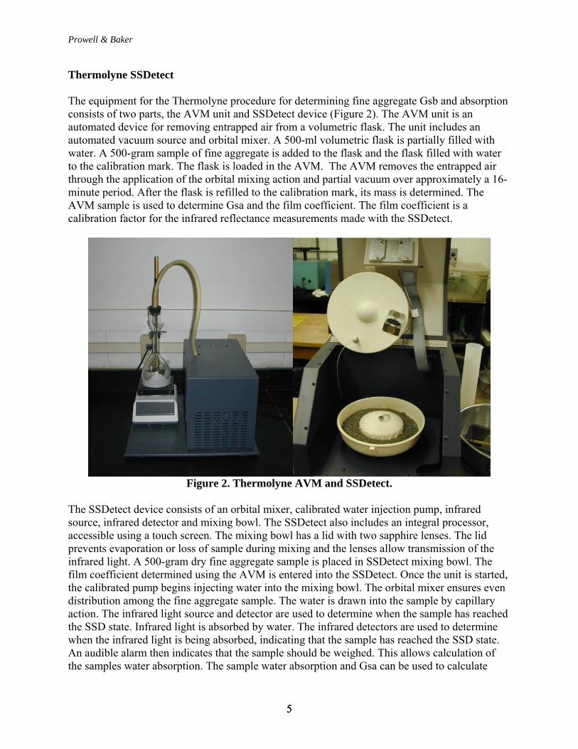
Thermolyne SSDetect The equipment for the Thermolyne procedure for determining fine aggregate Gsb and absorption consists of two parts, the AVM unit and SSDetect device (Figure 2). The AVM unit is an automated device for removing entrapped air from a volumetric flask. The unit includes an automated vacuum source and orbital mixer. A 500-ml volumetric flask is partially filled with water. A 500-gram sample of fine aggregate is added to the flask and the flask filled with water to the calibration mark. The flask is loaded in the AVM. The AVM removes the entrapped air through the application of the orbital mixing action and partial vacuum over approximately a 16-minute period. After the flask is refilled to the calibration mark, its mass is determined. The AVM sample is used to determine Gsa and the film coefficient. The film coefficient is a calibration factor for the infrared reflectance measurements made with the SSDetect.

Figure 2. Thermolyne AVM and SSDetect.

The SSDetect device consists of an orbital mixer, calibrated water injection pump, infrared source, infrared detector and mixing bowl. The SSDetect also includes an integral processor, accessible using a touch screen. The mixing bowl has a lid with two sapphire lenses. The lid prevents evaporation or loss of sample during mixing and the lenses allow transmission of the infrared light. A 500-gram dry fine aggregate sample is placed in SSDetect mixing bowl. The film coefficient determined using the AVM is entered into the SSDetect. Once the unit is started, the calibrated pump begins injecting water into the mixing bowl. The orbital mixer ensures even distribution among the fine aggregate sample. The water is drawn into the sample by capillary action. The infrared light source and detector are used to determine when the sample has reached the SSD state. Infrared light is absorbed by water. The infrared detectors are used to determine when the infrared light is being absorbed, indicating that the sample has reached the SSD state. An audible alarm then indicates that the sample should be weighed. This allows calculation of the samples water absorption. The sample water absorption and Gsa can be used to calculate

Prowell & Baker

6 6

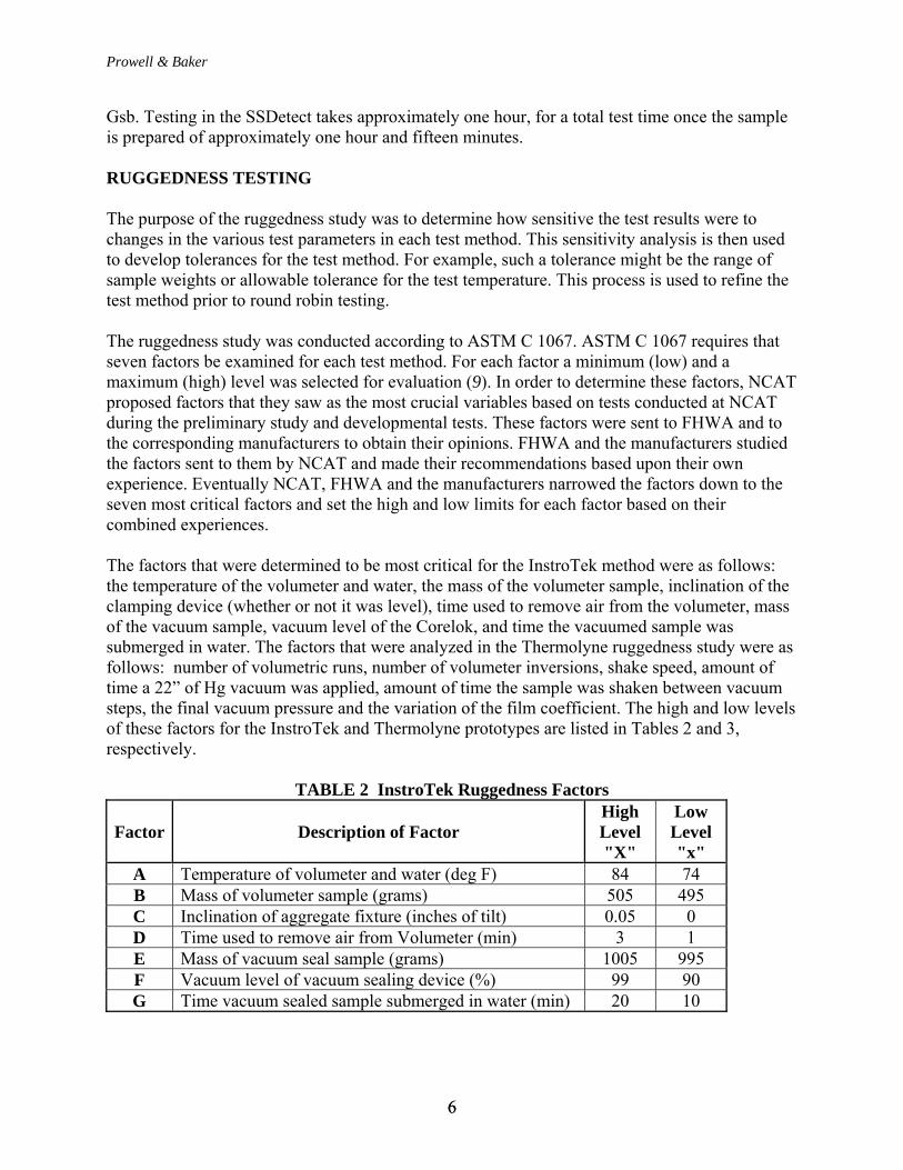
Gsb. Testing in the SSDetect takes approximately one hour, for a total test time once the sample is prepared of approximately one hour and fifteen minutes. RUGGEDNESS TESTING The purpose of the ruggedness study was to determine how sensitive the test results were to changes in the various test parameters in each test method. This sensitivity analysis is then used to develop tolerances for the test method. For example, such a tolerance might be the range of sample weights or allowable tolerance for the test temperature. This process is used to refine the test method prior to round robin testing. The ruggedness study was conducted according to ASTM C 1067. ASTM C 1067 requires that seven factors be examined for each test method. For each factor a minimum (low) and a maximum (high) level was selected for evaluation (9). In order to determine these factors, NCAT proposed factors that they saw as the most crucial variables based on tests conducted at NCAT during the preliminary study and developmental tests. These factors were sent to FHWA and to the corresponding manufacturers to obtain their opinions. FHWA and the manufacturers studied the factors sent to them by NCAT and made their recommendations based upon their own experience. Eventually NCAT, FHWA and the manufacturers narrowed the factors down to the seven most critical factors and set the high and low limits for each factor based on their combined experiences. The factors that were determined to be most critical for the InstroTek method were as follows: the temperature of the volumeter and water, the mass of the volumeter sample, inclination of the clamping device (whether or not it was level), time used to remove air from the volumeter, mass of the vacuum sample, vacuum level of the Corelok, and time the vacuumed sample was submerged in water. The factors that were analyzed in the Thermolyne ruggedness study were as follows: number of volumetric runs, number of volumeter inversions, shake speed, amount of time a 22” of Hg vacuum was applied, amount of time the sample was shaken between vacuum steps, the final vacuum pressure and the variation of the film coefficient. The high and low levels of these factors for the InstroTek and Thermolyne prototypes are listed in Tables 2 and 3, respectively.

TABLE 2 InstroTek Ruggedness Factors

Factor Description of Factor High Level "X"

Low Level "x"

A Temperature of volumeter and water (deg F) 84 74 B Mass of volumeter sample (grams) 505 495 C Inclination of aggregate fixture (inches of tilt) 0.05 0 D Time used to remove air from Volumeter (min) 3 1 E Mass of vacuum seal sample (grams) 1005 995 F Vacuum level of vacuum sealing device (%) 99 90 G Time vacuum sealed sample submerged in water (min) 20 10

Prowell & Baker

7 7

TABLE 3 Thermolyne Ruggedness Factors

Factor Description of Factor High Level "X"

Low Level "x"

A Number of volumetric runs 3 1 B Number of volumeter inversions 2 1 C Maxi Mix III shake speed (RPM) 2200 1500 D Time 22" vacuum is pulled (min) 5 0 E Time used to shake b/w vacuum steps (min) 5 2 F Final vacuum pressure (inches of Hg) 27 25 G How far the film coefficient is varied from actual 0 -3

ASTM C 1067 requires that 16 determinations be conducted with the factors. A determination is a prescribed combination of these factors. In this case, there were 8 different combinations evaluated. Each combination was replicated for a total of 16 determinations. This represents a 1/16th partial fraction (27-4) with two replicates. The factor level combinations for each determination are shown in Appendix A, Tables A-1 and A-2. After the factors for each test method were evaluated, they were used to set tolerance ranges for future testing. ASTM C 1067 also recommends that three labs be used during the investigation, especially if one of the labs performed the initial development work on the prototype. Using two additional labs also helped clarify the instructions in the test methods and made sure that the results were not biased. The three labs that participated in the ruggedness study for the InstroTek prototype were FHWA, InstroTek and NCAT. The same labs were used for the Thermolyne ruggedness study except Thermolyne participated instead of InstroTek. In order to get an overall idea of how each prototype would react to a wide range of materials, three different material types were used: limestone (material A), diabase (material B) and natural sand (material E). These three material types were chosen because of their great differences in angularities and dust contents (percent passing 0.075 mm (No. 200) sieve) as seen in Table 1. Material B had the highest dust content with a dust content of 7.5 percent whereas Material E had the lowest dust content (0.9 percent). Material E also had the lowest angularity with a fine aggregate angularity value of 41.2 percent. Materials A and B had similar angularities with fine aggregate angularities of 47.5 and 48.8 percent according to AASHTO T-304, respectively. InstroTek Ruggedness Results The test results for the InstroTek ruggedness study are presented in Appendix A, Table A-3. Because of the different factor level combinations used for each determination, observation of the results themselves is difficult. However, it was noticed that Lab 1 had much higher absorption results in determinations 1, 2, 7, and 8 for both replicates for materials A and E. This coincided with lower bulk specific gravity results. At first, it was thought that Lab 1 might be an outlier, but after comparing determination 1 of replicate 1 with determination 1 of replicate 2 and so on, a trend appeared. Factor D coincided with the different results. Even though Lab 1

Prowell & Baker

8 8

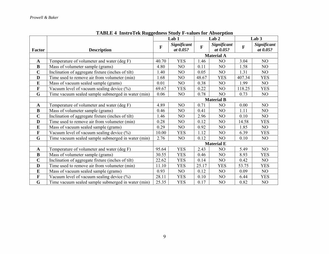
differed from the other two labs, all three had consistent results; meaning that each lab’s replicate one determination results were similar to that lab’s replicate two determination results. For example, Labs 1, 2, and 3 had absorption results of 5.91, 3.85, and 3.27, respectively, for determination 2 of replicate one and for replicate two of determination 2 they had values of 5.73, 3.56, and 3.92, respectively. This suggested that Lab 1 was doing something different, but consistently different. Table A-1 was then examined to determine what factors were different for these four determinations (1, 2, 7, and 8) as compared to the remaining four. It was noticed that Laboratory 1 determined a higher absorption when Factor D, the time to remove the air in the volumeter, was at the high level (3 minutes). From talking with the operators of the tests, it was determined that the method of stirring the sample to remove the air was the cause of this trend. The procedure required that the samples be stirred by inserting the spatula and pulling it to the center of the bowl and repeating this process at 45 degree increments. It was determined that Lab 1 stirred the samples only 8 times where, Labs 2 and 3 stirred the samples continuously until the appropriate time period (1 or 3 minutes) had elapsed. When performing a 3-minute test (determinations 1, 2, 7 and 8), continuous stirring removed more entrapped air and may have allowed the aggregate to absorb more water, both of which result in a smaller bulk volume because the process measures the displacement of water. The more water an aggregate absorbs, the less volume it displaces. In determinations 3, 4, 5 and 6, Lab 3’s absorption results were higher than the other two labs in most cases. This was also thought to be an effect of the stirring method used, but it could not be determined if this was the only factor that caused this trend. A modified version of a spreadsheet developed by Hall (10) was used to analyze the data according to ASTM C 1067. ASTM C 1067 uses an F-test to evaluate the effect of the seven factors. If an F value greater than 5.59 was calculated for a factor, then that factor was said to cause a significant effect at the 5 percent level (95 percent confidence) (11). If the F value for a given factor was 5.59 or less NO was reported, meaning that this factor was not significant. There are nine results (three materials x three labs) for each property analyzed (absorption, bulk specific gravity and apparent specific gravity). The results of these properties are described below in detail. Percent Absorption Examining the F-values for absorption in Table 4, one first notices that the time to remove the air in the volumeter (Factor D) and the vacuum level (Factor F) of the Corelok were the most significant factors. Both factors had results that were significant in six of nine cases. Taking a closer look at the time to remove entrapped air results, it was noticed that material E was significant for all labs, material A was significant for two of the three labs and material B was significant in only one case. Since materials A and E had absorptions of about 5 and 2 percent, respectively, high absorptive materials appeared to have the greatest effect on the time used to remove air. Another contribution to the significant differences for Factor F was caused by the different stirring methods described previously.

Prowell & Baker

9

TABLE 4 InstroTek Ruggedness Study F-values for Absorption Lab 1 Lab 2 Lab 3

Factor

Description F Significant at 0.05? F Significant

at 0.05? F Significant at 0.05?

Material A A Temperature of volumeter and water (deg F) 40.70 YES 1.46 NO 3.04 NO B Mass of volumeter sample (grams) 4.80 NO 0.11 NO 1.58 NO C Inclination of aggregate fixture (inches of tilt) 1.40 NO 0.05 NO 1.31 NO D Time used to remove air from volumeter (min) 1.68 NO 48.67 YES 407.34 YES E Mass of vacuum sealed sample (grams) 0.01 NO 0.38 NO 1.99 NO F Vacuum level of vacuum sealing device (%) 69.67 YES 0.22 NO 118.25 YES G Time vacuum sealed sample submerged in water (min) 0.06 NO 0.78 NO 0.73 NO

Material B A Temperature of volumeter and water (deg F) 4.89 NO 0.71 NO 0.00 NO B Mass of volumeter sample (grams) 0.46 NO 0.41 NO 1.11 NO C Inclination of aggregate fixture (inches of tilt) 1.46 NO 2.96 NO 0.10 NO D Time used to remove air from volumeter (min) 0.28 NO 0.12 NO 14.58 YES E Mass of vacuum sealed sample (grams) 0.29 NO 0.92 NO 1.85 NO F Vacuum level of vacuum sealing device (%) 10.00 YES 1.12 NO 6.39 YES G Time vacuum sealed sample submerged in water (min) 2.76 NO 0.12 NO 0.10 NO

Material E A Temperature of volumeter and water (deg F) 95.64 YES 2.43 NO 5.49 NO B Mass of volumeter sample (grams) 30.55 YES 0.46 NO 8.93 YES C Inclination of aggregate fixture (inches of tilt) 22.62 YES 0.14 NO 0.42 NO D Time used to remove air from volumeter (min) 11.10 YES 25.17 YES 53.75 YES E Mass of vacuum sealed sample (grams) 0.93 NO 0.12 NO 0.09 NO F Vacuum level of vacuum sealing device (%) 28.11 YES 0.10 NO 6.44 YES G Time vacuum sealed sample submerged in water (min) 25.35 YES 0.17 NO 0.82 NO

Prowell & Baker

10

The vacuum level of the Corelok device was significant for two of the three labs for all three materials (six of nine cases). All six cases occurred with Labs 1 and 3. Changing the vacuum level from 99 to 98 percent resulted in significant differences for all materials for Labs 1 and 3. Since Lab 2 did not have any significant differences, it was thought that Lab 2’s Corelok device was not obtaining the correct or the same vacuum levels. The mass of the vacuum-sealed sample (Factor G) had no significant differences between levels. This was expected since this factor was not directly related to the absorption results. The inclination of the aggregate fixture (Factor C) and the time that the sample was submerged in water (Factor G) were significant in only one of the nine cases. The significant case for both factors occurred with Lab 1 for material E. Therefore, these two factors were not considered to have significant effects. The volumeter and volumeter water temperature (Factor A) and the mass of the volumeter sample (Factor B) were significant in two of the nine cases. These factors were both significant for Material E tested by Lab 1. It should be noted that Lab 1 changed the ambient temperature of the room to the prescribed bulk determination test temperatures (74 and 84oF) for materials B and E. Changing the ambient temperature should not affect any of the other factors examined in this study; therefore Lab 1’s results were not eliminated from the evaluation. Material E was a highly absorptive material; it was thought that this along with the changing of the ambient temperature caused a significant difference in material E’s results for Lab 1. Since Lab 1 changed the ambient temperature, another study on just temperature effects was conducted. It is described later in the evaluation of significant factors section. Bulk Specific Gravity The F-values for each lab and material for bulk specific gravity are shown in Table 5. The bulk specific gravity results coincided with the absorption results since the calculation of the bulk specific gravity was dependent on absorption. As with absorption, the time to remove air in the volumeter (Factor D) proved to be the most significant factor. It was significant in six of the nine cases. There were significant differences for materials A and E in five of those six cases whereas; there was only one significant case for material B. As described previously, the stirring method used and the absorption capacity of the aggregates appeared to cause the significant differences. Volumeter and water temperature (Factor A) was the next most influential factor having significant differences in four of the nine cases. Materials A and B had just one lab each with significant differences and material E had two labs with significant differences for this factor. Since two of these significant differences were produced by Lab 1 (materials A and E), a reasonable conclusion could not be made because Lab 1 changed the ambient room temperature. Therefore, this factor was investigated further in the reevaluation of factors section described below. Next, the mass of the volumeter sample (Factor B) and the inclination of the aggregate fixture (Factor C) had significant differences in only two of nine and one of nine cases, respectively. All of these differences occurred with material E and two of the three cases were produced by the Lab 1. These two cases could have been caused by the fact that Lab 1 changed the ambient temperature of the room, as described previously, when conducting these tests.

Prowell & Baker

11

TABLE 5 InstroTek Ruggedness Study F-values for Bulk Specific Gravity Lab 1 Lab 2 Lab 3

Factor

Description F Significant at 0.05? F Significant

at 0.05? F Significant at 0.05?

Material A A Temperature of volumeter and water (deg F) 37.50 YES 1.07 NO 3.11 NO B Mass of volumeter sample (grams) 1.36 NO 0.01 NO 0.99 NO C Inclination of aggregate fixture (inches of tilt) 0.41 NO 0.01 NO 0.74 NO D Time used to remove air from volumeter (min) 1.93 NO 102.27 YES 492.86 YES E Mass of vacuum sealed sample (grams) 0.01 NO 0.17 NO 2.65 NO F Vacuum level of vacuum sealing device (%) 16.16 YES 0.43 NO 46.61 YES

G Time vacuum sealed sample submerged in water (min) 0.07 NO 0.34 NO 1.18 NO

Material B A Temperature of volumeter and water (deg F) 2.65 NO 7.81 YES 0.03 NO B Mass of volumeter sample (grams) 0.00 NO 0.05 NO 1.29 NO C Inclination of aggregate fixture (inches of tilt) 1.35 NO 2.52 NO 0.06 NO D Time used to remove air from volumeter (min) 0.18 NO 1.46 NO 17.64 YES E Mass of vacuum sealed sample (grams) 0.49 NO 0.09 NO 2.03 NO F Vacuum level of vacuum sealing device (%) 0.95 NO 0.02 NO 1.92 NO

G Time vacuum sealed sample submerged in water (min) 0.62 NO 0.05 NO 0.06 NO

Material E A Temperature of volumeter and water (deg F) 71.92 YES 2.44 NO 5.61 YES B Mass of volumeter sample (grams) 17.49 YES 0.42 NO 11.57 YES C Inclination of aggregate fixture (inches of tilt) 18.15 YES 0.23 NO 0.61 NO D Time used to remove air from volumeter (min) 9.06 YES 26.90 YES 65.41 YES E Mass of vacuum sealed sample (grams) 0.18 NO 0.03 NO 0.02 NO F Vacuum level of vacuum sealing device (%) 18.15 YES 0.01 NO 2.76 NO

G Time vacuum sealed sample submerged in water (min) 21.63 YES 0.39 NO 2.14 NO

Prowell & Baker

12

The mass of the vacuum-sealed sample (Factor E) was the only factor that had no significant differences. The vacuum level of the Corelok (Factor F) had significant differences occur in three of the nine cases. Two of these cases occurred with material A with the remaining case occurring with material E. This indicated that changes in vacuum levels for high absorption materials could cause a difference in the results since materials A and E were considered to be highly absorptive materials. Since the bulk specific gravity is related to the apparent specific gravity and absorption, a definite conclusion could not be made solely from the bulk specific gravity results. Therefore, the apparent specific gravity results for this factor were further examined, as discussed later, to better define the cause of variation for this factor. Finally, the time the sample was submerged in the water (Factor G) had only one significant difference. This difference occurred with material E when tested by Lab 1. Apparent Specific Gravity As described previously, a test consists of a bulk volume determination and an apparent specific gravity determination. During the apparent specific gravity determination a vacuum is pulled on a separate 1000g sample and then the sample is placed underwater, where water is introduced to the sample as described previously. During this evaluation there were four factors that occurred in the bulk determination that were analyzed as follows: volumeter and volumeter water temperature, mass of volumeter sample, inclination of aggregate fixture and the amount of time required to remove air in the volumeter. These factors (A, B, C, and D) in the bulk determination should not cause any significant differences in the apparent specific gravity since the two are not directly related. However, three significant differences occurred during the apparent determinations that were related to the determination of bulk specific gravity as seen in Table 6. Two of these differences occurred with the mass of the volumeter sample (Factor B) and the other one occurred with the volumeter and volumeter water temperature (Factor A). All three of these differences were produced by the same lab (Lab 1) and occurred with the higher absorptive materials (A and E). Therefore, it was concluded that lab error might be the cause. The other two factors, inclination of aggregate fixture (Factor C) and the amount of time to remove air in the volumeter (Factor D), as expected had no significant differences. In the apparent specific gravity determination, the vacuum level of the Corelok device (Factor F) proved to be the most significant factor. Significant differences occurred in six of the nine cases. All six of the cases occurred with materials A, B and E for Labs 1 and 3. This was a result of the higher vacuum level enabling more water to fill the permeable voids of the aggregate. Lab 2 did not have any significant differences for any of the materials. This could be a result of Lab 2’s vacuum not obtaining the same vacuum levels as the other two labs. The mass of the vacuum-sealed sample (Factor E) and the time the sample was submerged in water (Factor G) both had only one significant difference. These differences occurred with material E in both cases.

Additional Investigation of Significant Factors for InstroTek Procedure After reviewing the data as a whole, it was observed that the vacuum level of the Corelok and the time to remove air in the volumeter were the factors that caused the most variation in the results. The vacuum level influenced the apparent specific gravity and water absorption the most whereas; the time to remove air in the volumeter influenced the bulk specific gravity and the water absorption. InstroTek, FHWA and NCAT decided to conduct additional tests on these

Prowell & Baker

13

TABLE 6 InstroTek Ruggedness Study F-values for Apparent Specific Gravity Lab 1 Lab 2 Lab 3

Factor

Description F Significant at 0.05? F Significant

at 0.05? F Significant at 0.05?

Material A A Temperature of volumeter and water (deg F) 0.34 NO 1.63 NO 1.17 NO B Mass of volumeter sample (grams) 16.52 YES 0.90 NO 5.03 NO C Inclination of aggregate fixture (inches of tilt) 4.87 NO 0.21 NO 3.65 NO D Time used to remove air from volumeter (min) 0.34 NO 0.77 NO 0.56 NO E Mass of vacuum sealed sample (grams) 0.34 NO 0.73 NO 3.04 NO F Vacuum level of vacuum sealing device (%) 291.45 YES 0.02 NO 667.04 YES

G Time vacuum sealed sample submerged in water (min) 0.12 NO 1.57 NO 1.17 NO

Material B A Temperature of volumeter and water (deg F) 0.51 NO 0.16 NO 1.61 NO B Mass of volumeter sample (grams) 0.51 NO 0.69 NO 0.03 NO C Inclination of aggregate fixture (inches of tilt) 0.00 NO 1.39 NO 0.63 NO D Time used to remove air from volumeter (min) 1.85 NO 1.08 NO 1.61 NO E Mass of vacuum sealed sample (grams) 3.05 NO 0.81 NO 0.10 NO F Vacuum level of vacuum sealing device (%) 8.48 YES 1.23 NO 112.63 YES

G Time vacuum sealed sample submerged in water (min) 1.21 NO 0.11 NO 0.40 NO

Material E A Temperature of volumeter and water (deg F) 14.20 YES 0.99 NO 2.48 NO B Mass of volumeter sample (grams) 19.32 YES 0.99 NO 0.23 NO C Inclination of aggregate fixture (inches of tilt) 1.58 NO 1.00 NO 0.00 NO D Time used to remove air from volumeter (min) 0.89 NO 1.01 NO 0.23 NO E Mass of vacuum sealed sample (grams) 7.99 YES 1.01 NO 0.57 NO F Vacuum level of vacuum sealing device (%) 11.93 YES 0.99 NO 42.26 YES

G Time vacuum sealed sample submerged in water (min) 0.00 NO 1.01 NO 7.12 YES

Prowell and Baker

14

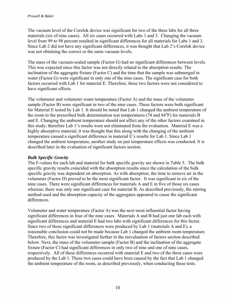
factors using tighter tolerances and focusing on the material/materials that posed the most variation in the test results to reduce the variability of the test method. The vacuum levels examined in this study were 98 and 99 percent vacuum. As described previously, the results indicated that changing the vacuum level by one percent caused a significant difference in the results. The only way that this can be accomplished is by manually changing the setting. Therefore, requiring the Corelok to be set at a 99 percent vacuum level alleviated this variation in the results. This idea worked because the Corelok will keep running until the desired vacuum level is obtained. However, this approach did not consider the amount of dwell time used. The dwell time is the period of time the vacuum is held once the desired vacuum level is achieved. To address the dwell time issue, a study of different dwell times was conducted. The study used material A (limerock) because it gave the most variable results during the ruggedness study. The study included three labs (InstroTek, FHWA, and NCAT) with each lab evaluating three different dwell times (0, 15, and 30 seconds). In order to obtain a true idea as to how the dwell time affected the apparent results, the volumeter results were kept constant for all labs. This helped show the true variation of the dwell times. The results are shown in Table 7. Practically speaking, there appears to be little consistent difference as a function of dwell time. Analysis of variance (ANOVA) was performed to analyze the results using apparent specific gravity as the

TABLE 7 ASG Results for Dwell Time Evaluation

Dwell Time

Apparent Specific Gravity

(sec) Lab 1 Lab 2 Lab 3 0 2.700 2.688 2.694 0 2.702 2.690 2.699 0 2.706 2.696 2.694 0 2.701 2.689 2.693 0 2.703 2.695 2.696

Average 2.702 2.692 2.695 Std. 0.002 0.004 0.002 15 2.707 2.701 2.705 15 2.705 2.697 2.707 15 2.703 2.689 2.704 15 2.699 2.691 2.698 15 2.696 2.691 2.708

Average 2.702 2.694 2.704 Std. 0.004 0.005 0.004 30 2.705 2.689 2.705 30 2.701 2.694 2.707 30 2.698 2.693 2.700 30 2.697 2.689 2.707 30 2.697 2.693 2.703

Average 2.700 2.692 2.704 Std. 0.003 0.002 0.003

Prowell and Baker

15

response variable and dwell time and lab as factors. The results indicate that dwell time, lab and the interaction between dwell time and lab were all significant. Lab was the most significant effect (F-value = 32.78, p-value = 0.000), followed by the interaction between dwell time and lab (F-value = 4.44, p-value = 0.000) and dwell time was the least significant factor (F-value = 4.12, p-value = 0.025). Tukey’s pair-wise comparisons indicated that the average apparent specific gravity for the 15 second dwell time was significantly different from the apparent specific gravity for zero dwell time, but there were no significant differences for the other pair-wise comparisons. Based on these analyses, a minimum 15 second dwell time was selected for the round robin test procedure.

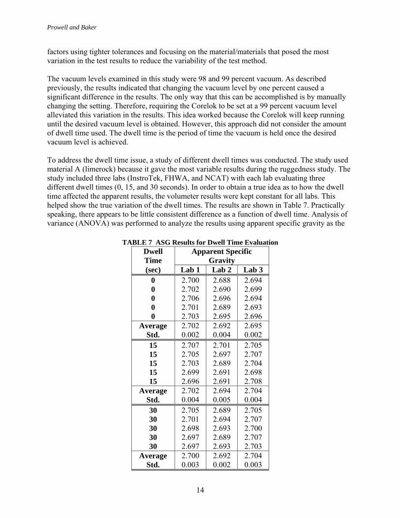
A small secondary study was also conducted to further evaluate the volumeter and volumeter water temperature. As with the previous factor, only the most variable material from the ruggedness study was evaluated (Material E). The same three labs were used. The vacuum sample results were held constant to better obtain the true variance of the volumeter data. A temperature strip was also added to the outside of the volumeter so that the temperature could be recorded (Figure 3).

Figure 3. Volumeter with Temperature Strip.

All three labs were instructed to conduct the volumeter test within 2 +/- 0.5 minutes. Labs 1 and 2 tested five samples at 70°F and 76oF and Lab 3 tested five samples at 68oF and 78oF. Two temperature ranges were evaluated in order to determine which one would produce the most repeatable results. The results are shown in Table 8. Lab 3 conducted tests at 73 +/- 5oF and Labs 1 and 2 conducted tests at 73 +/- 3oF. ANOVA was conducted using either absorption or bulk specific gravity (Gsb) as responses and volumeter temperature and lab as factors for Labs 1 and 2’s results. ANOVA indicated that the +/- 3°F range used by Labs 1 and 2 did not result in significant differences for either water absorption or

Prowell and Baker

16

bulk specific gravity. Therefore, tests conducted at 70 oF and 76 oF would not result in significant differences in the results.

TABLE 8 Volumeter and Volumeter Water Temperature Evaluation Temperature Lab 1 Lab 2 Temperature Lab 3

(°F) % Absorption Gsb

% Absorption Gsb (°F) % Absorption Gsb

70 2.10 2.523 2.41 2.503 68 3.30 2.451 70 1.86 2.538 2.41 2.503 68 2.99 2.470 70 1.90 2.535 2.41 2.503 68 2.72 2.486 70 1.98 2.530 2.53 2.495 68 2.19 2.520 70 1.94 2.533 2.41 2.503 68 3.08 2.464

Average 1.95 2.532 2.44 2.501 Average 2.86 2.478 Std. 0.091 0.006 0.053 0.004 Std. 0.426 0.027 76 2.29 2.510 2.53 2.495 78 2.32 2.511 76 2.29 2.510 2.57 2.493 78 2.50 2.500 76 2.45 2.500 2.37 2.505 78 2.19 2.520 76 1.98 2.530 2.41 2.503 78 2.23 2.517 76 1.86 2.538 2.49 2.498 78 2.37 2.509

Average 2.18 2.518 2.48 2.499 Average 2.32 2.511 Std. 0.247 0.016 0.082 0.005 Std. 0.122 0.008

However, the +/- 5°F volumeter temperature range used by Lab 3 resulted in significant differences for both absorption and bulk specific gravity. Based on these analyses, the volumeter temperature tolerance was set at +/- 3°F. Thermolyne SSDetect Ruggedness Results The test results for the Thermolyne SSDetect ruggedness study are presented in Appendix A, Table A-4. Because of the different factor level combinations used for each determination, observation of the results themselves is difficult. As with the InstroTek ruggedness study, ASTM C 1067 was followed to calculate F-statistics for evaluation of the factor level combinations using a modified version of a spreadsheet developed by Hall (10). If the calculated F value was 5.59 or less a NO was reported, meaning that that factor was not significant. The results for the seven factors are described below in detail.

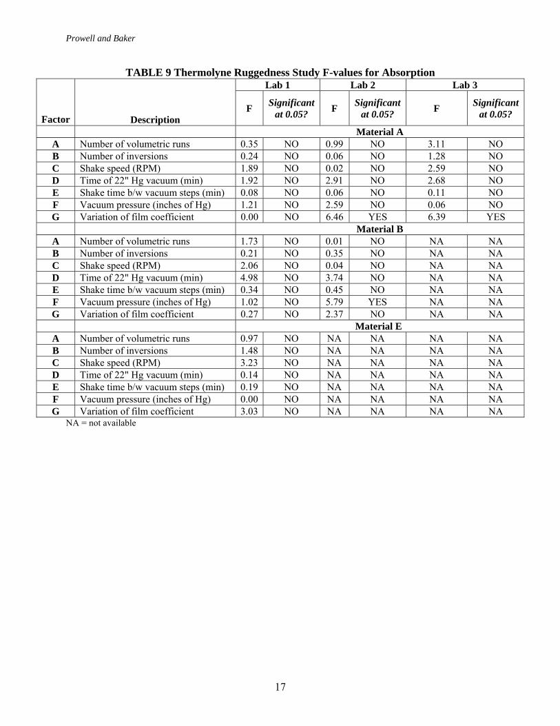
Note that only one lab completed ruggedness testing on all three materials, the second lab completed the ruggedness testing for two of the three materials (Material A and B) and a the third lab completed ruggedness testing on only a single material (Material A). Percent Absorption and Bulk Specific Gravity The bulk specific gravity and absorption were affected by a few of the factors examined in this study as seen in Tables 9 and 10. This indicated that the tolerances used for the factors during this study did not significantly affect the absorption and bulk specific gravity values.

Prowell and Baker

17

TABLE 9 Thermolyne Ruggedness Study F-values for Absorption Lab 1 Lab 2 Lab 3

Factor

Description F Significant

at 0.05? F Significant at 0.05? F Significant

at 0.05?

Material A A Number of volumetric runs 0.35 NO 0.99 NO 3.11 NO B Number of inversions 0.24 NO 0.06 NO 1.28 NO C Shake speed (RPM) 1.89 NO 0.02 NO 2.59 NO D Time of 22" Hg vacuum (min) 1.92 NO 2.91 NO 2.68 NO E Shake time b/w vacuum steps (min) 0.08 NO 0.06 NO 0.11 NO F Vacuum pressure (inches of Hg) 1.21 NO 2.59 NO 0.06 NO G Variation of film coefficient 0.00 NO 6.46 YES 6.39 YES

Material B A Number of volumetric runs 1.73 NO 0.01 NO NA NA B Number of inversions 0.21 NO 0.35 NO NA NA C Shake speed (RPM) 2.06 NO 0.04 NO NA NA D Time of 22" Hg vacuum (min) 4.98 NO 3.74 NO NA NA E Shake time b/w vacuum steps (min) 0.34 NO 0.45 NO NA NA F Vacuum pressure (inches of Hg) 1.02 NO 5.79 YES NA NA G Variation of film coefficient 0.27 NO 2.37 NO NA NA

Material E A Number of volumetric runs 0.97 NO NA NA NA NA B Number of inversions 1.48 NO NA NA NA NA C Shake speed (RPM) 3.23 NO NA NA NA NA D Time of 22" Hg vacuum (min) 0.14 NO NA NA NA NA E Shake time b/w vacuum steps (min) 0.19 NO NA NA NA NA F Vacuum pressure (inches of Hg) 0.00 NO NA NA NA NA G Variation of film coefficient 3.03 NO NA NA NA NA

NA = not available

Prowell and Baker

18

TABLE 10 Thermolyne Ruggedness Study F-values for Bulk Specific Gravity Lab 1 Lab 2 Lab 3

Factor

Description F Significant at 0.05? F Significant

at 0.05? F Significant at 0.05?

Material A A Number of volumetric runs 0.14 NO 1.25 NO 2.44 NO B Number of inversions 0.36 NO 0.28 NO 1.34 NO C Shake speed (RPM) 1.91 NO 0.20 NO 2.84 NO D Time of 22" Hg vacuum (min) 1.69 NO 2.39 NO 2.23 NO E Shake time b/w vacuum steps (min) 0.00 NO 0.08 NO 0.20 NO F Vacuum pressure (inches of Hg) 0.39 NO 1.72 NO 0.01 NO G Variation of film coefficient 0.05 NO 7.19 YES 5.72 YES

Material B A Number of volumetric runs 2.39 NO 0.00 NO NA NA B Number of inversions 0.39 NO 0.02 NO NA NA C Shake speed (RPM) 1.43 NO 0.00 NO NA NA D Time of 22" Hg vacuum (min) 3.97 NO 4.06 NO NA NA E Shake time b/w vacuum steps (min) 0.13 NO 0.45 NO NA NA F Vacuum pressure (inches of Hg) 0.24 NO 4.90 NO NA NA G Variation of film coefficient 0.19 NO 4.47 NO NA NA

Material E A Number of volumetric runs 0.90 NO NA NA NA NA B Number of inversions 1.20 NO NA NA NA NA C Shake speed (RPM) 2.45 NO NA NA NA NA D Time of 22" Hg vacuum (min) 0.05 NO NA NA NA NA E Shake time b/w vacuum steps (min) 0.14 NO NA NA NA NA F Vacuum pressure (inches of Hg) 0.02 NO NA NA NA NA G Variation of film coefficient 3.02 NO NA NA NA NA

NA = not available

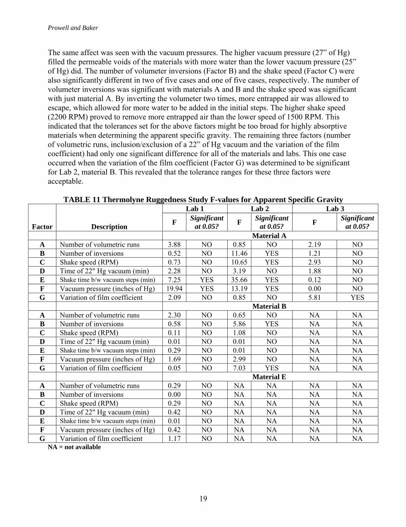
The variation of the film coefficient (Factor G) was one of the factors that showed up as being significant for BSG and absorption. However, this factor was only significant in one of five cases for both properties. Both of these cases occurred with material B. The vacuum pressure (factor F) was another factor that resulted in a significant result. In Table 9, vacuum pressure was significant in one of five cases for absorption (Material B). Therefore, these factors were regarded as significantly affecting the test results. Apparent Specific Gravity In Table 11, one first notices that the most significant differences occurred with material A. Material A is a highly absorptive limerock. Results for material A were especially influenced by the variation of the shaking time (Factor E) and final vacuum pressure (Factor F). These two factors were significant for all labs with material A. This demonstrated that the two levels used for both of these two factors caused a significant difference in the results when testing highly absorptive materials. The short shaking time of 2 minutes proved to be too short to remove all of the entrapped air. The 5-minute time allowed for more water to be absorbed, thus allowing more air to be removed.

Prowell and Baker

19

The same affect was seen with the vacuum pressures. The higher vacuum pressure (27” of Hg) filled the permeable voids of the materials with more water than the lower vacuum pressure (25” of Hg) did. The number of volumeter inversions (Factor B) and the shake speed (Factor C) were also significantly different in two of five cases and one of five cases, respectively. The number of volumeter inversions was significant with materials A and B and the shake speed was significant with just material A. By inverting the volumeter two times, more entrapped air was allowed to escape, which allowed for more water to be added in the initial steps. The higher shake speed (2200 RPM) proved to remove more entrapped air than the lower speed of 1500 RPM. This indicated that the tolerances set for the above factors might be too broad for highly absorptive materials when determining the apparent specific gravity. The remaining three factors (number of volumetric runs, inclusion/exclusion of a 22” of Hg vacuum and the variation of the film coefficient) had only one significant difference for all of the materials and labs. This one case occurred when the variation of the film coefficient (Factor G) was determined to be significant for Lab 2, material B. This revealed that the tolerance ranges for these three factors were acceptable.

TABLE 11 Thermolyne Ruggedness Study F-values for Apparent Specific Gravity

Lab 1 Lab 2 Lab 3 Factor

Description F Significant at 0.05? F Significant

at 0.05? F Significant at 0.05?

Material A A Number of volumetric runs 3.88 NO 0.85 NO 2.19 NO B Number of inversions 0.52 NO 11.46 YES 1.21 NO C Shake speed (RPM) 0.73 NO 10.65 YES 2.93 NO D Time of 22" Hg vacuum (min) 2.28 NO 3.19 NO 1.88 NO E Shake time b/w vacuum steps (min) 7.25 YES 35.66 YES 0.12 NO F Vacuum pressure (inches of Hg) 19.94 YES 13.19 YES 0.00 NO G Variation of film coefficient 2.09 NO 0.85 NO 5.81 YES

Material B A Number of volumetric runs 2.30 NO 0.65 NO NA NA B Number of inversions 0.58 NO 5.86 YES NA NA C Shake speed (RPM) 0.11 NO 1.08 NO NA NA D Time of 22" Hg vacuum (min) 0.01 NO 0.01 NO NA NA E Shake time b/w vacuum steps (min) 0.29 NO 0.01 NO NA NA F Vacuum pressure (inches of Hg) 1.69 NO 2.99 NO NA NA G Variation of film coefficient 0.05 NO 7.03 YES NA NA

Material E A Number of volumetric runs 0.29 NO NA NA NA NA B Number of inversions 0.00 NO NA NA NA NA C Shake speed (RPM) 0.29 NO NA NA NA NA D Time of 22" Hg vacuum (min) 0.42 NO NA NA NA NA E Shake time b/w vacuum steps (min) 0.01 NO NA NA NA NA F Vacuum pressure (inches of Hg) 0.42 NO NA NA NA NA G Variation of film coefficient 1.17 NO NA NA NA NA

NA = not available

Prowell and Baker

20

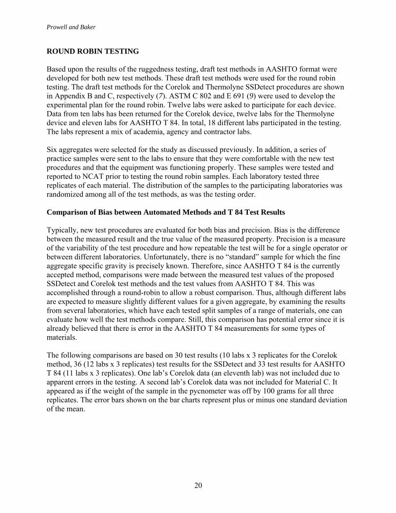
ROUND ROBIN TESTING Based upon the results of the ruggedness testing, draft test methods in AASHTO format were developed for both new test methods. These draft test methods were used for the round robin testing. The draft test methods for the Corelok and Thermolyne SSDetect procedures are shown in Appendix B and C, respectively (7). ASTM C 802 and E 691 (9) were used to develop the experimental plan for the round robin. Twelve labs were asked to participate for each device. Data from ten labs has been returned for the Corelok device, twelve labs for the Thermolyne device and eleven labs for AASHTO T 84. In total, 18 different labs participated in the testing. The labs represent a mix of academia, agency and contractor labs. Six aggregates were selected for the study as discussed previously. In addition, a series of practice samples were sent to the labs to ensure that they were comfortable with the new test procedures and that the equipment was functioning properly. These samples were tested and reported to NCAT prior to testing the round robin samples. Each laboratory tested three replicates of each material. The distribution of the samples to the participating laboratories was randomized among all of the test methods, as was the testing order. Comparison of Bias between Automated Methods and T 84 Test Results Typically, new test procedures are evaluated for both bias and precision. Bias is the difference between the measured result and the true value of the measured property. Precision is a measure of the variability of the test procedure and how repeatable the test will be for a single operator or between different laboratories. Unfortunately, there is no “standard” sample for which the fine aggregate specific gravity is precisely known. Therefore, since AASHTO T 84 is the currently accepted method, comparisons were made between the measured test values of the proposed SSDetect and Corelok test methods and the test values from AASHTO T 84. This was accomplished through a round-robin to allow a robust comparison. Thus, although different labs are expected to measure slightly different values for a given aggregate, by examining the results from several laboratories, which have each tested split samples of a range of materials, one can evaluate how well the test methods compare. Still, this comparison has potential error since it is already believed that there is error in the AASHTO T 84 measurements for some types of materials. The following comparisons are based on 30 test results (10 labs x 3 replicates for the Corelok method, 36 (12 labs x 3 replicates) test results for the SSDetect and 33 test results for AASHTO T 84 (11 labs x 3 replicates). One lab’s Corelok data (an eleventh lab) was not included due to apparent errors in the testing. A second lab’s Corelok data was not included for Material C. It appeared as if the weight of the sample in the pycnometer was off by 100 grams for all three replicates. The error bars shown on the bar charts represent plus or minus one standard deviation of the mean.

Prowell and Baker

21

0.0

1.0

2.0

3.0

4.0

5.0

6.0

7.0

8.0

A B C D E FMaterial

Wat

er A

bsor

ptio

n, P

erce

ntCorelokSSDetectT84

A

B B

C BA

CB A

A

BC

B A

B

A

B AB

Figure 4. Average Water Absorption by Material and Method.

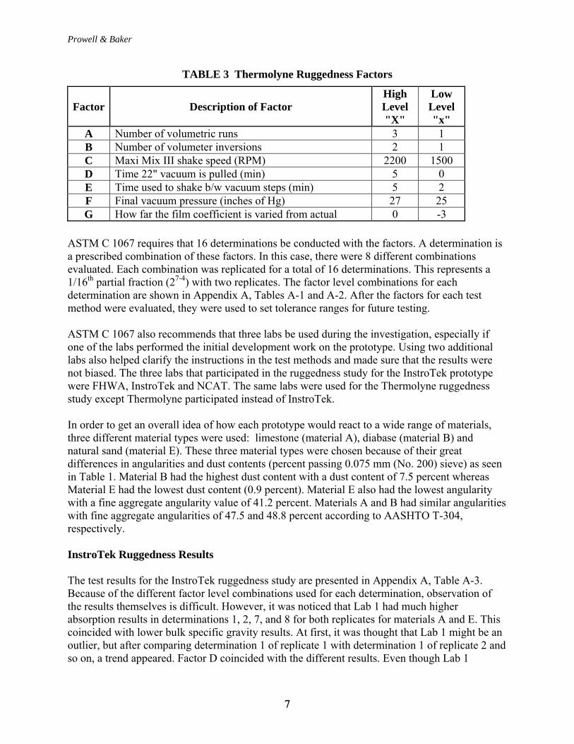
Water Absorption Figure 4 shows a comparison of the average water absorption results by material and method. There appear to be some large differences between the water absorption values determined by AASHTO T 84 and those determined by the new methods. ANOVA analyses using the General Linear Model and Tukey’s comparisons were performed for each material (11). Percent water absorption was used as the response variable and laboratory and method were used as factors. The results are illustrated as A, B, AB or C in Figure 4. Results with the same letter are not significantly different at the 5 percent level of significance. The AASHTO T 84 results for material F are denoted “AB”; this indicates that the AASHTO T 84 results are not statistically different from either the Corelok (A) or the SSDetect (B) results. However, the Corelok and SSDetect results are different from one another. When tested by material, the Corelok and the SSDetect water absorptions were both statistically different from AASHTO T 84 in four of six cases. The results from AASHTO T 84 and the two new methods were similar for the two natural sands (Materials E and F). The absorption values measured by the SSDetect and Corelok methods were larger than the values for AASHTO T 84 for the limerock, slag and both natural sands. The absorption values measured by the SSDetect and Corelok methods were both smaller than the values for AASHTO T 84 for the washed diabase. The angularity and relatively high dust content of the two diabase materials (B and C) make it difficult to obtain a slump when determining the SSD condition according to AASHTO T 84. The aggregate producer for materials B and C reports that the absorption of the coarse aggregate is typically 0.47 percent (12). It was anticipated that AASHTO T 84 would underestimate the water absorption for such materials.

Prowell and Baker

22

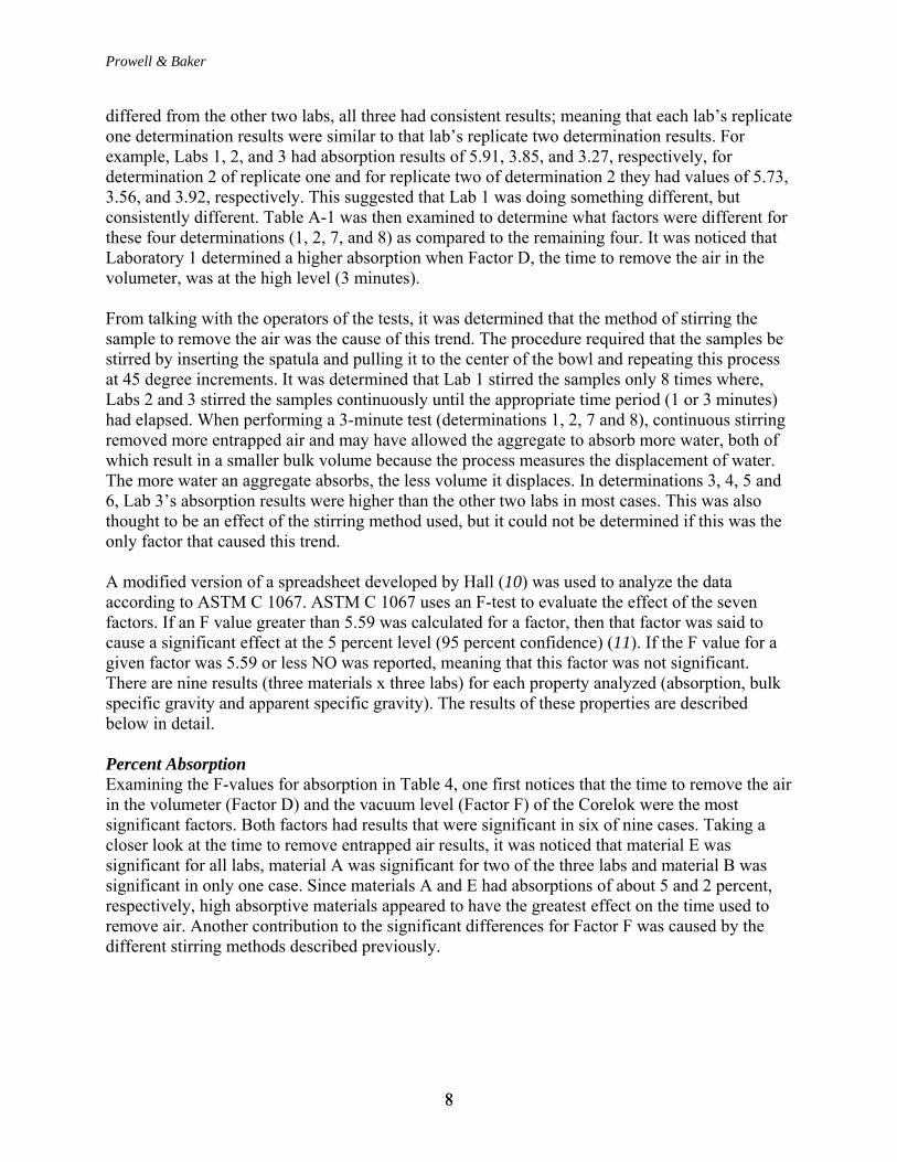
For samples for which it is difficult to obtain a slump, AASHTO T 84 indicates that if fines become airborne when a portion of the sample is dropped from four to six inches that a partial slump may be used to indicate the SSD point. Further, Note 2 in AASHTO T 84 discusses alternate procedures for determining the SSD point (1). The test results indicate that these alternate AASHTO T 84 procedures may actually overestimate the water absorption. The SSDetect water absorption is also higher than the coarse aggregate for material C with 14.7 percent passing the No. 200 sieve. The Corelok device produced much higher water absorptions for both material A (limerock) and material D (slag). It is expected that the rate of absorption on these two materials is so high as to cause errors when determining the bulk volume of the sample, even when the pycnometer portion is completed in two minutes. Apparent Specific Gravity Figure 5 shows a comparison of the average Gsa results by material and method. Similar to water absorption, ANOVA and Tukey’s tests were performed using the Gsa results as the response and both method and laboratory as factors. The results are illustrated as A, B, C or AB in Figure 5. When tested by material, both the Corelok and SSDetect Gsa values were statistically different from AASHTO T 84 in four of six cases. The Corelok method was different than AASHTO T 84 for the same four materials as indicated by the water absorption results. The Gsa results measured by the SSDetect and Corelok methods were both larger than AASHTO T 84 for the limerock and slag. This may be due to the vacuum used by both methods causing a greater portion of the aggregate void structure to be filled with water. The Gsa results measured by the

2.300

2.400

2.500

2.600

2.700

2.800

2.900

3.000

3.100

A B C D E FMaterial

Gsa

CorelokSSDetectT84

A B C

B BA B B A

AB

B

A BAB A

BA

Figure 5. Average Gsa by Material and Method.

Prowell and Baker

23

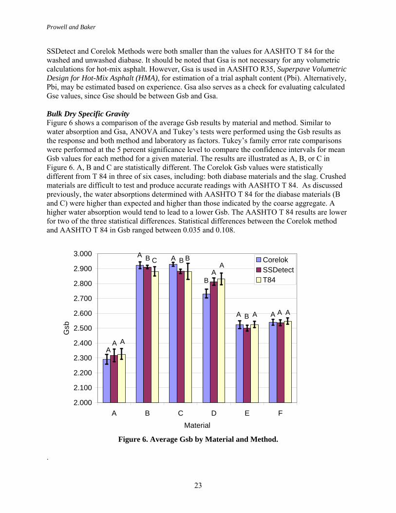
SSDetect and Corelok Methods were both smaller than the values for AASHTO T 84 for the washed and unwashed diabase. It should be noted that Gsa is not necessary for any volumetric calculations for hot-mix asphalt. However, Gsa is used in AASHTO R35, Superpave Volumetric Design for Hot-Mix Asphalt (HMA), for estimation of a trial asphalt content (Pbi). Alternatively, Pbi, may be estimated based on experience. Gsa also serves as a check for evaluating calculated Gse values, since Gse should be between Gsb and Gsa. Bulk Dry Specific Gravity Figure 6 shows a comparison of the average Gsb results by material and method. Similar to water absorption and Gsa, ANOVA and Tukey’s tests were performed using the Gsb results as the response and both method and laboratory as factors. Tukey’s family error rate comparisons were performed at the 5 percent significance level to compare the confidence intervals for mean Gsb values for each method for a given material. The results are illustrated as A, B, or C in Figure 6. A, B and C are statistically different. The Corelok Gsb values were statistically different from T 84 in three of six cases, including: both diabase materials and the slag. Crushed materials are difficult to test and produce accurate readings with AASHTO T 84. As discussed previously, the water absorptions determined with AASHTO T 84 for the diabase materials (B and C) were higher than expected and higher than those indicated by the coarse aggregate. A higher water absorption would tend to lead to a lower Gsb. The AASHTO T 84 results are lower for two of the three statistical differences. Statistical differences between the Corelok method and AASHTO T 84 in Gsb ranged between 0.035 and 0.108.

2.000

2.100

2.200

2.300

2.400

2.500

2.600

2.700

2.800

2.900

3.000

A B C D E FMaterial

Gsb

CorelokSSDetectT84

AA A

A B C A B B

BA

A

A B A A A A

Figure 6. Average Gsb by Material and Method.

.

Prowell and Baker

24

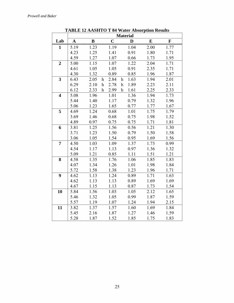
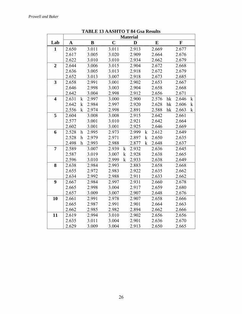
The SSDetect values were statistically different from the T 84 values in three of six cases for the washed diabase, rounded natural sand and angular natural sand. Statistical differences between the SSDetect Method and AASHTO T 84 ranged from 0.016 to 0.030. Where statistical differences occurred, the differences were larger than for the Corelok Method. Both the Corelok and the SSDetect produced larger Gsb values for the washed diabase than the values for AASHTO T 84. Precision of Test Methods ASTM E 691 software (13) was used to determine the precision of the test methods from the round robin results. Precision of the test method has two components, repeatability and reproducibility. Repeatability (Sr) is the within-laboratory standard deviation of the test results. Reproducibility (SR) is the between-laboratory standard deviation of the test results. ASTM E 691 (13) uses two statistics to analyze the data for consistency: h and k. The h statistic is an indicator of how one laboratory’s average for a material compares with the average of the other laboratories. The h statistic is based on Student’s t test. The k statistic is an indicator of how one laboratory’s variability for a given set of replicate samples compares with that of all the other laboratories. The k statistic is based on the F ratio. AASHTO T 84 The round robin results for absorption, Gsa and Gsb are presented in Tables 12, 13 and 14, respectively. If a cell’s (one lab’s results for one material) average was significantly different from the average of the other cells, an h is shown beside the data in the table. If a cell’s variability or standard deviation is significantly different from the pooled variability of the remaining cells, a k is shown beside the data in the table. Plots of the h values for each cell are shown by lab in Appendix D, Figures D-1, D-2 and D-3 for absorption, Gsa and Gsb, respectively. It should be noted that the h values may be positive or negative. Positive h values indicate that the cell’s average is larger than the average of the other labs results, whereas negative h values indicate that the cell’s average is less than the average of the other cells results. These graphs were inspected to identify any trends which might indicate systematic errors in testing by a lab. Lab 3’s water absorption results were consistently high. The h statistics for two of six of Lab 3’s materials (B and C) were larger than the critical value. This indicates that the SSD weights measured by Lab 3 were consistently high. These consistently high SSD weights affect the measured Gsb. Figure D-3 indicates that Lab 3’s Gsb values were consistently lower than the other labs. Table 14 indicates that the h statistic for material C was larger than the critical value. Based on these analyses, Lab 3’s data were considered to be outliers when determining the precision of the water absorption measurements.

Prowell and Baker

25

TABLE 12 AASHTO T 84 Water Absorption Results Material

Lab A B C D E F 1 5.19 1.23 1.19 1.04 2.00 1.77 4.23 1.25 1.41 0.91 1.80 1.71 4.59 1.27 1.07 0.66 1.73 1.95 2 5.00 1.15 1.07 1.22 2.04 1.71 4.61 1.05 1.05 0.91 2.35 1.71 4.30 1.32 0.89 0.85 1.96 1.87 3 6.43 2.05 h 2.84 h 1.63 1.94 2.01 6.29 2.10 h 2.78 h 1.89 2.23 2.11 6.12 2.33 h 2.99 h 1.61 2.25 2.33 4 5.08 1.96 1.01 1.36 1.94 1.73 5.44 1.40 1.17 0.79 1.32 1.96 5.06 1.23 1.65 0.77 1.77 1.67 5 4.69 1.24 0.68 1.01 1.75 1.79 3.69 1.46 0.68 0.75 1.98 1.52 4.89 0.97 0.75 0.75 1.71 1.81 6 3.81 1.25 1.56 0.56 1.21 1.30 3.71 1.23 1.50 0.79 1.50 1.58 3.06 1.05 1.54 0.95 1.69 1.56 7 4.50 1.03 1.09 1.37 1.73 0.99 4.54 1.17 1.13 0.97 1.36 1.32 5.09 1.21 0.85 1.11 1.51 1.21 8 4.58 1.35 1.76 1.06 1.85 1.83 4.07 1.34 1.26 1.01 1.98 1.84 5.72 1.58 1.38 1.23 1.96 1.71 9 4.62 1.13 1.24 0.89 1.71 1.63 4.62 1.13 1.13 0.89 1.69 1.69 4.67 1.15 1.13 0.87 1.73 1.54

10 5.84 1.56 1.03 1.05 2.12 1.65 5.46 1.32 1.05 0.99 1.87 1.59 5.57 1.19 1.07 1.24 1.94 2.15

11 3.82 1.37 1.57 1.60 1.69 1.84 5.45 2.16 1.87 1.27 1.46 1.59 5.28 1.87 1.52 1.85 1.75 1.83

Prowell and Baker

26

TABLE 13 AASHTO T 84 Gsa Results Material

Lab A B C D E F 1 2.650 3.011 3.011 2.913 2.669 2.677 2.617 3.005 3.020 2.909 2.664 2.676 2.622 3.010 3.010 2.934 2.662 2.679 2 2.644 3.006 3.015 2.904 2.672 2.668 2.636 3.005 3.013 2.918 2.672 2.679 2.652 3.013 3.007 2.918 2.673 2.685 3 2.658 2.991 3.001 2.902 2.653 2.667 2.646 2.998 3.003 2.904 2.658 2.668 2.642 3.004 2.998 2.912 2.656 2.671 4 2.631 k 2.997 3.000 2.900 2.576 hk 2.646 k 2.642 k 2.984 2.997 2.920 2.628 hk 2.606 k 2.556 k 2.974 2.998 2.891 2.588 hk 2.663 k 5 2.604 3.008 3.008 2.915 2.642 2.661 2.577 3.001 3.010 2.921 2.642 2.664 2.602 3.001 3.001 2.925 2.646 2.669 6 2.528 h 2.995 2.973 2.999 k 2.612 2.649 2.528 h 2.979 2.971 2.897 k 2.650 2.635 2.498 h 2.993 2.988 2.877 k 2.648 2.637 7 2.589 3.007 2.939 k 2.932 2.636 2.645 2.587 3.019 3.007 k 2.928 2.638 2.665 2.596 3.010 2.999 k 2.933 2.638 2.649 8 2.638 2.984 2.993 2.883 2.658 2.668 2.655 2.972 2.983 2.922 2.635 2.662 2.634 2.992 2.988 2.911 2.633 2.662 9 2.667 2.984 2.997 2.931 2.660 2.678 2.665 2.998 3.004 2.917 2.659 2.680 2.657 3.009 3.007 2.907 2.648 2.676

10 2.661 2.991 2.978 2.907 2.658 2.666 2.665 2.987 2.991 2.901 2.664 2.663 2.662 2.985 2.982 2.894 2.662 2.666

11 2.619 2.994 3.010 2.902 2.656 2.656 2.635 3.011 3.004 2.901 2.636 2.670 2.629 3.009 3.004 2.913 2.650 2.665

Prowell and Baker

27

TABLE 14 AASHTO T 84 Gsb Results Material

Lab A B C D E F 1 2.329 2.903 2.907 2.827 2.534 2.556 2.356 2.896 2.896 2.834 2.542 2.559 2.340 2.899 2.917 2.878 2.545 2.546 2 2.335 2.905 2.921 2.805 2.534 2.552 2.350 2.913 2.920 2.843 2.514 2.562 2.381 2.898 2.928 2.847 2.540 2.556 3 2.270 2.818 2.766 h 2.770 2.524 2.531 2.269 2.820 2.772 h 2.753 2.510 2.526 2.274 2.807 2.752 h 2.781 2.506 2.514 4 2.321 2.831 2.912 2.790 2.454 hk 2.530 k 2.310 2.865 2.895 2.854 2.540 hk 2.480 k 2.263 2.868 2.857 2.828 2.474 hk 2.550 k 5 2.321 2.900 2.947 2.832 2.525 2.540 2.353 2.875 2.949 2.859 2.510 2.560 2.308 2.916 2.935 2.862 2.531 2.546 6 2.306 2.886 2.841 2.950 k 2.531 2.561 2.311 2.874 2.844 2.832 k 2.549 2.530 2.320 2.902 2.856 2.801 k 2.535 2.533 7 2.319 2.916 2.848 k 2.818 2.521 2.577 2.315 2.916 2.908 k 2.847 2.546 2.575 2.293 2.904 2.925 k 2.840 2.537 2.567 8 2.353 2.869 2.843 2.798 2.534 2.543 2.396 2.859 2.876 2.838 2.505 2.538 2.289 2.857 2.870 2.811 2.504 2.546 9 2.374 2.886 2.890 2.856 2.545 2.567 2.373 2.900 2.905 2.843 2.545 2.564 2.364 2.908 2.908 2.836 2.532 2.570

10 2.303 2.857 2.890 2.821 2.516 2.554 2.326 2.874 2.900 2.820 2.538 2.555 2.318 2.882 2.890 2.795 2.532 2.522

11 2.381 2.876 2.874 2.773 2.542 2.532 2.304 2.827 2.845 2.798 2.538 2.561 2.309 2.849 2.873 2.764 2.533 2.541

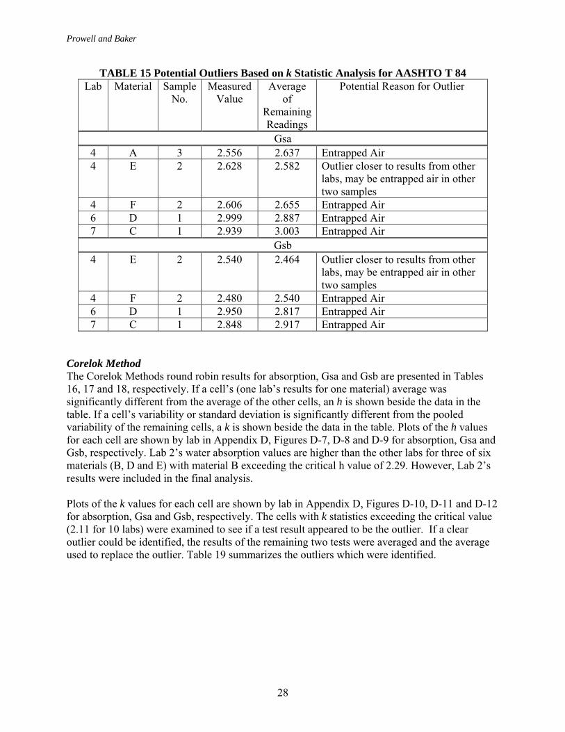
Plots of the k values for each cell are shown by lab in Appendix D, Figures D-4, D-5 and D-6 for absorption, Gsa and Gsb, respectively. The cells with k statistics exceeding the critical value (2.13 for 11 labs) were examined to see if a test result appeared to be the outlier. If a clear outlier could be identified, the results of the remaining two tests were averaged and the average used to replace the outlier. Table 15 summarizes the outliers which were identified. It is interesting to note that the outliers associated with AASHTO T 84 appear to result from improper removal of entrapped air in the pycnometer when determining the Gsa.

Prowell and Baker

28

TABLE 15 Potential Outliers Based on k Statistic Analysis for AASHTO T 84 Lab Material Sample

No. Measured

Value Average

of Remaining Readings

Potential Reason for Outlier

Gsa 4 A 3 2.556 2.637 Entrapped Air 4 E 2 2.628 2.582 Outlier closer to results from other

labs, may be entrapped air in other two samples

4 F 2 2.606 2.655 Entrapped Air 6 D 1 2.999 2.887 Entrapped Air 7 C 1 2.939 3.003 Entrapped Air

Gsb 4 E 2 2.540 2.464 Outlier closer to results from other

labs, may be entrapped air in other two samples

4 F 2 2.480 2.540 Entrapped Air 6 D 1 2.950 2.817 Entrapped Air 7 C 1 2.848 2.917 Entrapped Air

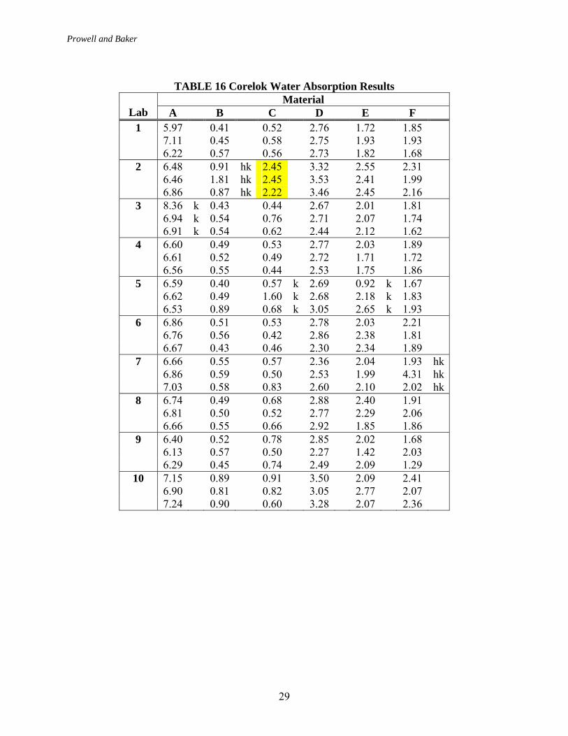
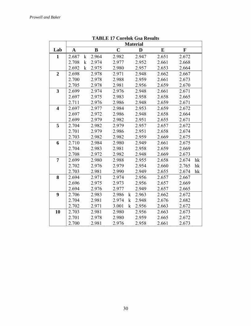
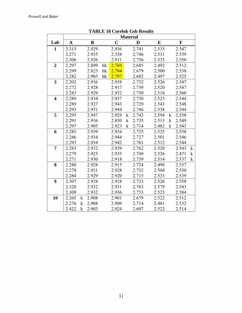
Corelok Method The Corelok Methods round robin results for absorption, Gsa and Gsb are presented in Tables 16, 17 and 18, respectively. If a cell’s (one lab’s results for one material) average was significantly different from the average of the other cells, an h is shown beside the data in the table. If a cell’s variability or standard deviation is significantly different from the pooled variability of the remaining cells, a k is shown beside the data in the table. Plots of the h values for each cell are shown by lab in Appendix D, Figures D-7, D-8 and D-9 for absorption, Gsa and Gsb, respectively. Lab 2’s water absorption values are higher than the other labs for three of six materials (B, D and E) with material B exceeding the critical h value of 2.29. However, Lab 2’s results were included in the final analysis. Plots of the k values for each cell are shown by lab in Appendix D, Figures D-10, D-11 and D-12 for absorption, Gsa and Gsb, respectively. The cells with k statistics exceeding the critical value (2.11 for 10 labs) were examined to see if a test result appeared to be the outlier. If a clear outlier could be identified, the results of the remaining two tests were averaged and the average used to replace the outlier. Table 19 summarizes the outliers which were identified.

Prowell and Baker

29

TABLE 16 Corelok Water Absorption Results

Material Lab A B C D E F

1 5.97 0.41 0.52 2.76 1.72 1.85 7.11 0.45 0.58 2.75 1.93 1.93 6.22 0.57 0.56 2.73 1.82 1.68 2 6.48 0.91 hk 2.45 3.32 2.55 2.31 6.46 1.81 hk 2.45 3.53 2.41 1.99 6.86 0.87 hk 2.22 3.46 2.45 2.16 3 8.36 k 0.43 0.44 2.67 2.01 1.81 6.94 k 0.54 0.76 2.71 2.07 1.74 6.91 k 0.54 0.62 2.44 2.12 1.62 4 6.60 0.49 0.53 2.77 2.03 1.89 6.61 0.52 0.49 2.72 1.71 1.72 6.56 0.55 0.44 2.53 1.75 1.86 5 6.59 0.40 0.57 k 2.69 0.92 k 1.67 6.62 0.49 1.60 k 2.68 2.18 k 1.83 6.53 0.89 0.68 k 3.05 2.65 k 1.93 6 6.86 0.51 0.53 2.78 2.03 2.21 6.76 0.56 0.42 2.86 2.38 1.81 6.67 0.43 0.46 2.30 2.34 1.89 7 6.66 0.55 0.57 2.36 2.04 1.93 hk 6.86 0.59 0.50 2.53 1.99 4.31 hk 7.03 0.58 0.83 2.60 2.10 2.02 hk 8 6.74 0.49 0.68 2.88 2.40 1.91 6.81 0.50 0.52 2.77 2.29 2.06 6.66 0.55 0.66 2.92 1.85 1.86 9 6.40 0.52 0.78 2.85 2.02 1.68 6.13 0.57 0.50 2.27 1.42 2.03 6.29 0.45 0.74 2.49 2.09 1.29

10 7.15 0.89 0.91 3.50 2.09 2.41 6.90 0.81 0.82 3.05 2.77 2.07 7.24 0.90 0.60 3.28 2.07 2.36

Prowell and Baker

30

TABLE 17 Corelok Gsa Results

Material Lab A B C D E F

1 2.687 k 2.964 2.982 2.947 2.651 2.672 2.708 k 2.974 2.977 2.952 2.661 2.668 2.692 k 2.975 2.980 2.957 2.653 2.664 2 2.698 2.978 2.971 2.948 2.662 2.667 2.700 2.978 2.988 2.959 2.661 2.673 2.705 2.978 2.981 2.956 2.659 2.670 3 2.699 2.974 2.976 2.948 2.661 2.671 2.697 2.975 2.983 2.958 2.658 2.665 2.711 2.976 2.986 2.948 2.659 2.671 4 2.697 2.977 2.984 2.953 2.659 2.672 2.697 2.972 2.986 2.948 2.658 2.664 2.699 2.979 2.982 2.951 2.655 2.671 5 2.704 2.982 2.979 2.957 2.657 2.672 2.701 2.979 2.986 2.951 2.658 2.674 2.703 2.982 2.982 2.959 2.669 2.675 6 2.710 2.984 2.980 2.949 2.661 2.675 2.704 2.983 2.981 2.958 2.659 2.669 2.708 2.972 2.982 2.948 2.669 2.673 7 2.699 2.980 2.988 2.955 2.658 2.674 hk 2.702 2.976 2.979 2.954 2.660 2.765 hk 2.703 2.981 2.990 2.949 2.655 2.674 hk 8 2.694 2.971 2.974 2.956 2.657 2.667 2.696 2.975 2.973 2.956 2.657 2.669 2.694 2.976 2.977 2.949 2.657 2.665 9 2.706 2.983 2.986 k 2.963 2.662 2.672 2.704 2.981 2.974 k 2.948 2.676 2.682 2.702 2.971 3.001 k 2.956 2.663 2.672

10 2.703 2.981 2.980 2.956 2.663 2.673 2.701 2.978 2.980 2.959 2.665 2.672 2.700 2.981 2.976 2.958 2.661 2.673

Prowell and Baker

31

TABLE 18 Corelok Gsb Results Material

Lab A B C D E F 1 2.315 2.929 2.936 2.741 2.535 2.547 2.271 2.935 2.358 2.746 2.531 2.539 2.306 2.926 2.931 2.736 2.533 2.550 2 2.297 2.899 hk 2.769 2.685 2.492 2.512 2.299 2.825 hk 2.784 2.679 2.500 2.538 2.282 2.903 hk 2.797 2.682 2.497 2.525 3 2.202 2.936 2.938 2.732 2.526 2.547 2.272 2.928 2.917 2.739 2.520 2.547 2.283 2.929 2.932 2.750 2.518 2.560 4 2.289 2.934 2.937 2.730 2.523 2.544 2.289 2.927 2.943 2.729 2.543 2.548 2.293 2.931 2.944 2.746 2.538 2.544 5 2.295 2.947 2.929 k 2.742 2.594 k 2.558 2.291 2.936 2.850 k 2.735 2.513 k 2.549 2.297 2.905 2.923 k 2.714 2.482 k 2.543 6 2.285 2.939 2.934 2.725 2.525 2.538 2.286 2.934 2.944 2.727 2.501 2.546 2.293 2.934 2.942 2.761 2.512 2.544 7 2.283 2.932 2.939 2.762 2.520 2.543 k 2.279 2.925 2.935 2.749 2.526 2.471 k 2.271 2.930 2.918 2.739 2.514 2.537 k 8 2.280 2.928 2.915 2.724 2.498 2.537 2.278 2.931 2.928 2.732 2.504 2.530 2.284 2.929 2.920 2.715 2.533 2.539 9 2.307 2.938 2.918 2.733 2.526 2.558 2.320 2.932 2.931 2.763 2.579 2.543 2.309 2.932 2.936 2.753 2.523 2.584

10 2.265 k 2.908 2.901 2.679 2.522 2.512 2.276 k 2.908 2.909 2.714 2.481 2.532 2.422 k 2.903 2.924 2.697 2.522 2.514

Prowell and Baker

32

TABLE 19 Potential Outliers Based on k Statistic Analysis for Corelok Method Lab Material Sample

No. Measured

Value Average

of Remaining Readings

Potential Reason for Outlier

Absorption 2 B 2 1.81 0.89 Mass of volumeter and sample low

by 1 gram possibly due to entrapped air

2 C All 2.45, 2.45, 2.22

0.611 Mass of volumeter and sample low, possibly due to entrapped air

3 A 1 8.36 6.93 Mass of volumeter and sample low, possibly due to entrapped air

5 C 2 1.60 0.63 No clear cause 5 E 1 0.92 2.42 Bag may have been touching tank 7 F 2 4.31 1.98 Submerged weight high

Gsa 7 F 2 2.765 2.674 Submerged weight high 9 C All 2.986,

2.974, 3.001

2.9811 Variable submerged weight

Gsb 2 B 2 2.825 2.901 Mass of volumeter and sample low

by 1 gram possibly due to entrapped air

2 C All 2.769, 2.784, 2.797

2.9031 Mass of volumeter and sample low, possibly due to entrapped air

5 C 2 2.850 2.926 No clear cause 5 E 1 2.594 2.498 Bag may have been touching tank 7 F 2 2.471 2.540 Submerged weight high 10 A 3 2.422 2.271 No clear cause

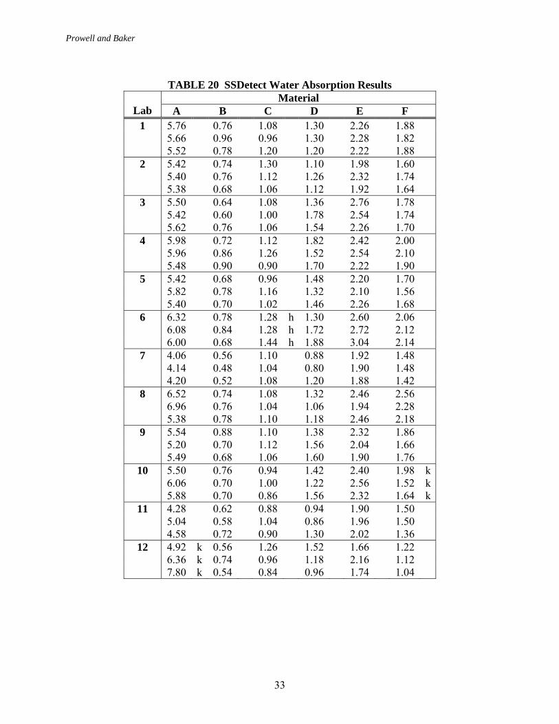
1 Average of remaining labs results. SSDetect The round robin results for absorption, Gsa and Gsb are presented in Tables 20, 21 and 22, respectively. If a cell’s (one lab’s results for one material) average was significantly different from the average of the other cells, an h is shown beside the data in the table. If a cell’s variability or standard deviation is significantly different from the pooled variability of the remaining cells, a k is shown beside the data in the table. Plots of the h values for each cell are shown by lab in Appendix D, Figures D-13, D-14 and D-15 for absorption, Gsa and Gsb, respectively.

Prowell and Baker

33

TABLE 20 SSDetect Water Absorption Results

Material Lab A B C D E F

1 5.76 0.76 1.08 1.30 2.26 1.88 5.66 0.96 0.96 1.30 2.28 1.82 5.52 0.78 1.20 1.20 2.22 1.88 2 5.42 0.74 1.30 1.10 1.98 1.60 5.40 0.76 1.12 1.26 2.32 1.74 5.38 0.68 1.06 1.12 1.92 1.64 3 5.50 0.64 1.08 1.36 2.76 1.78 5.42 0.60 1.00 1.78 2.54 1.74 5.62 0.76 1.06 1.54 2.26 1.70 4 5.98 0.72 1.12 1.82 2.42 2.00 5.96 0.86 1.26 1.52 2.54 2.10 5.48 0.90 0.90 1.70 2.22 1.90 5 5.42 0.68 0.96 1.48 2.20 1.70 5.82 0.78 1.16 1.32 2.10 1.56 5.40 0.70 1.02 1.46 2.26 1.68 6 6.32 0.78 1.28 h 1.30 2.60 2.06 6.08 0.84 1.28 h 1.72 2.72 2.12 6.00 0.68 1.44 h 1.88 3.04 2.14 7 4.06 0.56 1.10 0.88 1.92 1.48 4.14 0.48 1.04 0.80 1.90 1.48 4.20 0.52 1.08 1.20 1.88 1.42 8 6.52 0.74 1.08 1.32 2.46 2.56 6.96 0.76 1.04 1.06 1.94 2.28 5.38 0.78 1.10 1.18 2.46 2.18 9 5.54 0.88 1.10 1.38 2.32 1.86 5.20 0.70 1.12 1.56 2.04 1.66 5.49 0.68 1.06 1.60 1.90 1.76

10 5.50 0.76 0.94 1.42 2.40 1.98 k 6.06 0.70 1.00 1.22 2.56 1.52 k 5.88 0.70 0.86 1.56 2.32 1.64 k

11 4.28 0.62 0.88 0.94 1.90 1.50 5.04 0.58 1.04 0.86 1.96 1.50 4.58 0.72 0.90 1.30 2.02 1.36

12 4.92 k 0.56 1.26 1.52 1.66 1.22 6.36 k 0.74 0.96 1.18 2.16 1.12 7.80 k 0.54 0.84 0.96 1.74 1.04

Prowell and Baker

34

TABLE 21 SSDetect Gsa Results Materials

Lab A B C D E F 1 2.646 2.969 2.964 2.922 2.640 2.646 2.651 2.967 2.973 2.915 2.640 2.650 2.648 2.960 2.967 2.902 2.640 2.653 2 2.650 2.966 2.974 2.918 2.652 2.650 2.660 2.967 2.969 2.924 2.643 2.648 2.664 2.967 2.969 2.908 2.637 2.647 3 2.657 2.975 2.979 2.927 hk 2.643 2.654 2.662 2.980 2.974 3.036 hk 2.645 2.651 2.660 2.976 2.969 2.933 hk 2.647 2.651 4 2.655 2.976 2.971 2.916 2.652 2.656 2.664 2.967 2.974 2.911 2.647 2.659 2.661 2.974 2.973 2.911 2.643 2.657 5 2.648 k 2.971 2.966 2.921 2.646 2.660 2.632 k 2.970 2.966 2.915 2.650 2.655 2.650 k 2.971 2.975 2.926 2.658 2.651 6 2.654 2.969 2.971 2.931 2.651 2.653 2.650 2.974 2.972 2.927 2.653 2.653 2.652 2.972 2.969 2.933 2.653 2.654 7 2.660 2.974 2.976 2.941 2.654 2.653 2.661 2.969 2.974 2.929 2.654 2.655 2.661 2.969 2.976 2.924 2.647 2.658 8 2.668 2.967 2.982 2.924 2.644 2.662 2.668 2.980 2.976 2.936 2.651 2.664 2.670 2.980 2.982 2.915 2.654 2.662 9 2.651 2.973 2.969 2.912 2.648 2.650 2.655 2.969 2.964 2.921 2.641 2.655 2.660 2.973 2.969 2.927 2.651 2.650

10 2.668 2.974 2.973 2.931 2.646 2.662 2.662 2.969 2.985 2.921 2.646 2.653 2.665 2.982 2.978 2.924 2.655 2.655

11 2.667 2.980 2.981 2.941 2.656 2.659 2.666 2.979 2.983 2.922 2.650 2.656 2.665 2.983 2.980 2.924 2.649 2.658

12 2.657 2.970 2.969 2.909 2.625 k 2.656 2.661 2.973 2.977 2.919 2.648 k 2.650 2.655 2.970 2.974 2.921 2.648 k 2.658

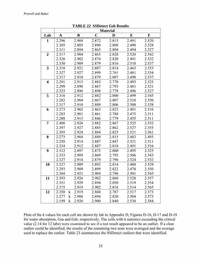
Prowell and Baker

35

TABLE 22 SSDetect Gsb Results Material

Lab A B C D E F 1 2.296 2.904 2.872 2.815 2.491 2.520 2.305 2.885 2.890 2.808 2.490 2.528 2.311 2.894 2.865 2.804 2.494 2.527 2 2.317 2.904 2.863 2.828 2.520 2.542 2.326 2.902 2.874 2.820 2.491 2.532 2.330 2.909 2.879 2.816 2.510 2.537 3 2.318 2.921 2.887 2.814 2.463 2.533 2.327 2.927 2.899 2.761 2.481 2.534 2.317 2.910 2.879 2.807 2.498 2.537 4 2.291 2.913 2.883 2.770 2.493 2.525 2.299 2.890 2.867 2.793 2.481 2.521 2.323 2.896 2.898 2.778 2.496 2.527 5 2.316 2.912 2.882 2.800 2.499 2.545 2.282 2.904 2.867 2.807 2.510 2.550 2.317 2.910 2.889 2.806 2.508 2.538 6 2.273 2.902 2.863 2.823 2.481 2.516 2.283 2.901 2.861 2.788 2.475 2.511 2.288 2.913 2.846 2.779 2.455 2.511 7 2.400 2.926 2.882 2.867 2.525 2.552 2.397 2.927 2.885 2.862 2.527 2.555 2.393 2.924 2.884 2.825 2.521 2.561 8 2.273 2.904 2.889 2.815 2.483 2.493 2.250 2.914 2.887 2.847 2.521 2.511 2.334 2.912 2.887 2.818 2.491 2.516 9 2.312 2.897 2.875 2.800 2.495 2.525 2.333 2.909 2.869 2.793 2.506 2.543 2.327 2.914 2.879 2.796 2.524 2.532

10 2.327 2.909 2.892 2.814 2.488 2.529 2.293 2.909 2.899 2.822 2.478 2.550 2.304 2.921 2.904 2.796 2.501 2.545

11 2.393 2.926 2.902 2.860 2.528 2.557 2.351 2.929 2.894 2.850 2.519 2.554 2.375 2.919 2.902 2.816 2.514 2.565

12 2.350 k 2.919 2.860 2.787 2.517 2.573 2.277 k 2.906 2.894 2.820 2.504 2.573 2.199 k 2.920 2.900 2.840 2.530 2.584

Plots of the k values for each cell are shown by lab in Appendix D, Figures D-16, D-17 and D-18 for water absorption, Gsa and Gsb, respectively. The cells with k statistics exceeding the critical value (2.14 for 12 labs) were examined to see if a test result appeared to be an outlier. If a clear outlier could be identified, the results of the remaining two tests were averaged and the average used to replace the outlier. Table 23 summarizes the SSDetect outliers that were identified.

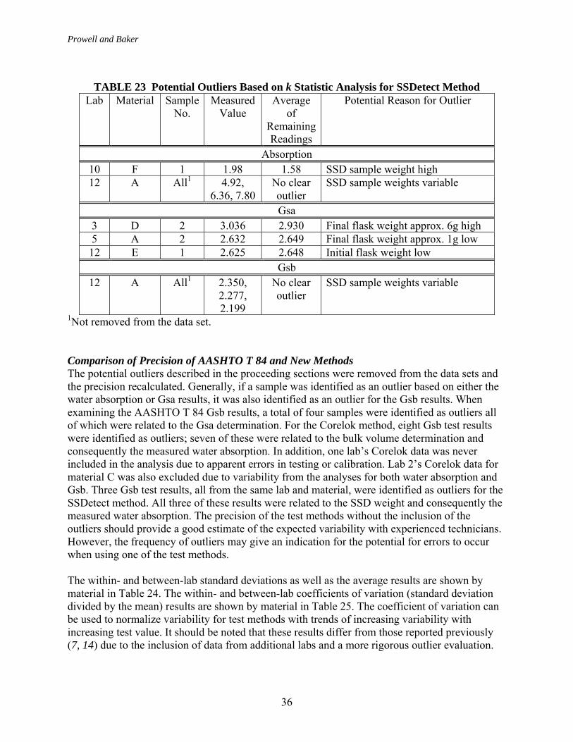
Prowell and Baker

36

TABLE 23 Potential Outliers Based on k Statistic Analysis for SSDetect Method

Lab Material Sample No.

Measured Value

Average of

Remaining Readings

Potential Reason for Outlier

Absorption 10 F 1 1.98 1.58 SSD sample weight high 12 A All1 4.92,

6.36, 7.80 No clear outlier

SSD sample weights variable

Gsa 3 D 2 3.036 2.930 Final flask weight approx. 6g high 5 A 2 2.632 2.649 Final flask weight approx. 1g low 12 E 1 2.625 2.648 Initial flask weight low

Gsb 12 A All1 2.350,

2.277, 2.199

No clear outlier

SSD sample weights variable

1Not removed from the data set. Comparison of Precision of AASHTO T 84 and New Methods The potential outliers described in the proceeding sections were removed from the data sets and the precision recalculated. Generally, if a sample was identified as an outlier based on either the water absorption or Gsa results, it was also identified as an outlier for the Gsb results. When examining the AASHTO T 84 Gsb results, a total of four samples were identified as outliers all of which were related to the Gsa determination. For the Corelok method, eight Gsb test results were identified as outliers; seven of these were related to the bulk volume determination and consequently the measured water absorption. In addition, one lab’s Corelok data was never included in the analysis due to apparent errors in testing or calibration. Lab 2’s Corelok data for material C was also excluded due to variability from the analyses for both water absorption and Gsb. Three Gsb test results, all from the same lab and material, were identified as outliers for the SSDetect method. All three of these results were related to the SSD weight and consequently the measured water absorption. The precision of the test methods without the inclusion of the outliers should provide a good estimate of the expected variability with experienced technicians. However, the frequency of outliers may give an indication for the potential for errors to occur when using one of the test methods. The within- and between-lab standard deviations as well as the average results are shown by material in Table 24. The within- and between-lab coefficients of variation (standard deviation divided by the mean) results are shown by material in Table 25. The coefficient of variation can be used to normalize variability for test methods with trends of increasing variability with increasing test value. It should be noted that these results differ from those reported previously (7, 14) due to the inclusion of data from additional labs and a more rigorous outlier evaluation.

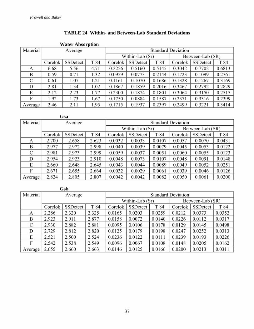
Prowell and Baker

37

TABLE 24 Within- and Between-Lab Standard Deviations

Water Absorption Standard Deviation Average

Within-Lab (Sr) Between-Lab (SR) Material

Corelok SSDetect T 84 Corelok SSDetect T 84 Corelok SSDetect T 84 A 6.68 5.56 4.71 0.2256 0.5160 0.5145 0.3042 0.7702 0.6813 B 0.59 0.71 1.32 0.0959 0.0773 0.2144 0.1723 0.1099 0.2761 C 0.61 1.07 1.21 0.1161 0.1070 0.1686 0.1328 0.1267 0.3169 D 2.81 1.34 1.02 0.1867 0.1859 0.2016 0.3467 0.2792 0.2829 E 2.12 2.23 1.77 0.2300 0.1874 0.1801 0.3064 0.3150 0.2515 F 1.92 1.73 1.67 0.1750 0.0884 0.1587 0.2371 0.3316 0.2399

Average 2.46 2.11 1.95 0.1715 0.1937 0.2397 0.2499 0.3221 0.3414 Gsa

Standard Deviation Average Within-Lab (Sr) Between-Lab (SR)

Material

Corelok SSDetect T 84 Corelok SSDetect T 84 Corelok SSDetect T 84 A 2.700 2.658 2.623 0.0032 0.0033 0.0107 0.0057 0.0070 0.0431 B 2.977 2.972 2.998 0.0040 0.0039 0.0079 0.0045 0.0053 0.0122 C 2.981 2.973 2.999 0.0059 0.0037 0.0051 0.0060 0.0055 0.0123 D 2.954 2.923 2.910 0.0048 0.0073 0.0107 0.0048 0.0091 0.0148 E 2.660 2.648 2.645 0.0043 0.0044 0.0089 0.0049 0.0052 0.0251 F 2.671 2.655 2.664 0.0032 0.0029 0.0061 0.0039 0.0046 0.0126

Average 2.824 2.805 2.807 0.0042 0.0042 0.0082 0.0050 0.0061 0.0200 Gsb

Standard Deviation Average Within-Lab (Sr) Between-Lab (SR)

Material

Corelok SSDetect T 84 Corelok SSDetect T 84 Corelok SSDetect T 84 A 2.286 2.320 2.325 0.0165 0.0203 0.0259 0.0212 0.0373 0.0352 B 2.923 2.911 2.877 0.0158 0.0072 0.0140 0.0226 0.0112 0.0317 C 2.930 2.882 2.881 0.0095 0.0106 0.0178 0.0129 0.0145 0.0498 D 2.729 2.812 2.820 0.0125 0.0179 0.0198 0.0247 0.0252 0.0313 E 2.521 2.500 2.524 0.0236 0.0122 0.0111 0.0239 0.0193 0.0226 F 2.542 2.538 2.549 0.0096 0.0067 0.0108 0.0148 0.0205 0.0162

Average 2.655 2.660 2.663 0.0146 0.0125 0.0166 0.0200 0.0213 0.0311

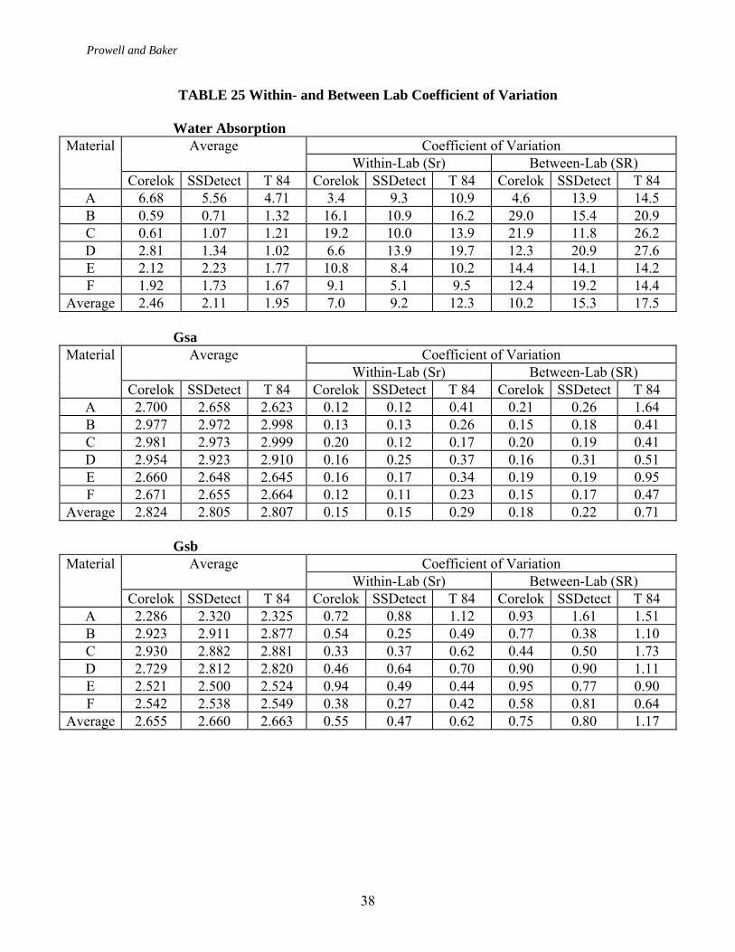
Prowell and Baker

38

TABLE 25 Within- and Between Lab Coefficient of Variation Water Absorption

Coefficient of Variation Average Within-Lab (Sr) Between-Lab (SR)

Material

Corelok SSDetect T 84 Corelok SSDetect T 84 Corelok SSDetect T 84 A 6.68 5.56 4.71 3.4 9.3 10.9 4.6 13.9 14.5 B 0.59 0.71 1.32 16.1 10.9 16.2 29.0 15.4 20.9 C 0.61 1.07 1.21 19.2 10.0 13.9 21.9 11.8 26.2 D 2.81 1.34 1.02 6.6 13.9 19.7 12.3 20.9 27.6 E 2.12 2.23 1.77 10.8 8.4 10.2 14.4 14.1 14.2 F 1.92 1.73 1.67 9.1 5.1 9.5 12.4 19.2 14.4

Average 2.46 2.11 1.95 7.0 9.2 12.3 10.2 15.3 17.5 Gsa

Coefficient of Variation Average Within-Lab (Sr) Between-Lab (SR)

Material

Corelok SSDetect T 84 Corelok SSDetect T 84 Corelok SSDetect T 84 A 2.700 2.658 2.623 0.12 0.12 0.41 0.21 0.26 1.64 B 2.977 2.972 2.998 0.13 0.13 0.26 0.15 0.18 0.41 C 2.981 2.973 2.999 0.20 0.12 0.17 0.20 0.19 0.41 D 2.954 2.923 2.910 0.16 0.25 0.37 0.16 0.31 0.51 E 2.660 2.648 2.645 0.16 0.17 0.34 0.19 0.19 0.95 F 2.671 2.655 2.664 0.12 0.11 0.23 0.15 0.17 0.47

Average 2.824 2.805 2.807 0.15 0.15 0.29 0.18 0.22 0.71 Gsb

Coefficient of Variation Average Within-Lab (Sr) Between-Lab (SR)

Material

Corelok SSDetect T 84 Corelok SSDetect T 84 Corelok SSDetect T 84 A 2.286 2.320 2.325 0.72 0.88 1.12 0.93 1.61 1.51 B 2.923 2.911 2.877 0.54 0.25 0.49 0.77 0.38 1.10 C 2.930 2.882 2.881 0.33 0.37 0.62 0.44 0.50 1.73 D 2.729 2.812 2.820 0.46 0.64 0.70 0.90 0.90 1.11 E 2.521 2.500 2.524 0.94 0.49 0.44 0.95 0.77 0.90 F 2.542 2.538 2.549 0.38 0.27 0.42 0.58 0.81 0.64

Average 2.655 2.660 2.663 0.55 0.47 0.62 0.75 0.80 1.17

Prowell and Baker

39

Material A, the high absorption limestone source, produced the largest within- and between-lab standard deviation for the water absorption results. For the SSDetect, this was due in part to the inclusion of Lab 12’s data, which had high variability but no clear single outlier. The within- and between-lab standard deviations for the water absorption results from AASHTO T 84 were also higher than the new methods for both of the diabase materials (B and C). It was expected that the high dust content and angular nature of the diabase would cause variability with AASHTO T 84. All three methods show a trend of increasing within- and between-lab variability with increasing water absorption. The within- and between-lab coefficient ofvariation (CV) or standard deviation divided by the mean, appears to be constant for the SSDetect water absorption results. The within- and between-lab standard deviations for the Gsa results from AASHTO T 84 were significantly higher than the new methods in all cases. As noted previously, when outliers were identified for AASHTO T 84, they were generally related to the determination of Gsa. The variability of the Gsa results from AASHTO T 84 were particularly large for materials A and E, the limestone and rounded natural sand. A trend of decreasing between-lab standard deviation with increasing Gsa was noted for AASHTO T 84, primarily driven by materials A and E. The within- and between-lab standard deviations for the Corelok and SSDetect methods as well as the within-lab standard deviation for AASHTO T 84 appear to be relatively constant regardless of the measured Gsa. The within- and between-lab standard deviations for Gsb determined from the AASHTO T 84 results are largest for the high absorption limestone (material A) and the unwashed diabase (materials C) and smallest for the two natural sands (materials E and F). The increased variability for crushed fines was expected and was one of the primary reasons for conducting this research. Such materials are more prevalent in hot-mix asphalt designs today than they were previously. Both new methods are generally more repeatable than AASHTO T 84. As mentioned previously, Lab 12’s SSDetect results, identified as outliers for material A, increased the between-lab standard deviation for material A. Recommended Precision Statements The recommended precision statements for the Corelok method, SSDetect method and AASHTO T 84 are shown in Table 26. The precision statements include the pooled within- and between-lab standard deviations (based on the sample variances) as well as the acceptable difference between two test results based on ASTM C 802 (9). The acceptable difference between two test results is the expected difference not to be exceeded with one chance in twenty for either two properly conducted tests by a single operator or two properly conducted tests by two different laboratories. The acceptable difference between two test results is referred to as the d2s. AASHTO T 84 reports a within-lab standard deviation of 0.11 and a between-lab standard deviation of 0.23 for water absorption (1). The precision statement included in AASHTO T 84 is based on materials with less than 1.0 percent absorption. The results from the current round robin, including materials with more than 4 percent water absorption are higher. The within-lab standard deviations for Gsa determined for AASHTO T 84 are less than (0.0095), while the between-lab standard deviation is slightly higher (0.020) as those reported in the test method. AASHTO T 84 reports a within-lab standard deviation of 0.011 and a between-lab standard

Prowell and Baker

40

deviation of 0.023 for Gsb. The results from the current round robin, including crushed materials regularly used in hot-mix asphalt are 40 to 50 percent higher.

TABLE 26 Recommended Precision Statements for Corelok, SSDetect and AASHTO T 84

Method Pooled Within-Lab Standard

Deviation

Pooled Between Lab

Standard Deviation

Within-Lab d2s Between-Lab d2s

Water Absorption Corelok 0.18 0.26 0.51 0.74 SSDetect 0.25 0.39 0.69 1.10

AASHTO T 84 0.27 0.37 0.76 1.06 Gsa

Corelok 0.0043 0.0050 0.012 0.014 SSDetect 0.0045 0.0063 0.013 0.018

AASHTO T 84 0.0085 0.0230 0.024 0.065 Gsb

Corelok 0.0154 0.0205 0.044 0.058 SSDetect 0.0135 0.0229 0.038 0.065

AASHTO T 84 0.0174 0.0329 0.049 0.093 All of the operators had significant experience with AASHTO T 84. Most operators were inexperienced with the Corelok and SSDetect methods. Based on the number of outliers identified, it appears that the Corelok test method requires more operator skill, particularly to remove entrapped air from the volumeter and to make sure the bag is properly weighed underwater. CONCLUSIONS Three new methods of determining fine aggregate specific gravity have been developed. Two of the methods, the Instrotek Corelok and Thermolyne SSDetect were evaluated in a round robin study. The third method was not evaluated pending further refinements to the procedure.

1. The Corelok and SSDetect methods of determining fine aggregate specific gravity offer significant timesavings over AASHTO T 84. Neither method requires the 16-hour soak period included in AASHTO T 84. This means that hot mix asphalt belt sweep samples could be taken to verify gravities during construction for volumetric calculations in a timely manner. Once a dry test sample is obtained the Corelok method can be completed in approximately 30 minutes and the SSDetect method can be completed in approximately 1 hour and 15 minutes.

2. Both the Corelok and SSDetect methods generally produce Gsb results that are similar to AASHTO T 84. Where statistical differences occurred for Gsb between the new methods and AASHTO T 84, the differences were smaller for the SSDetect method (Table 27). It is believed that AASHTO T 84 may not produce accurate results for angular materials

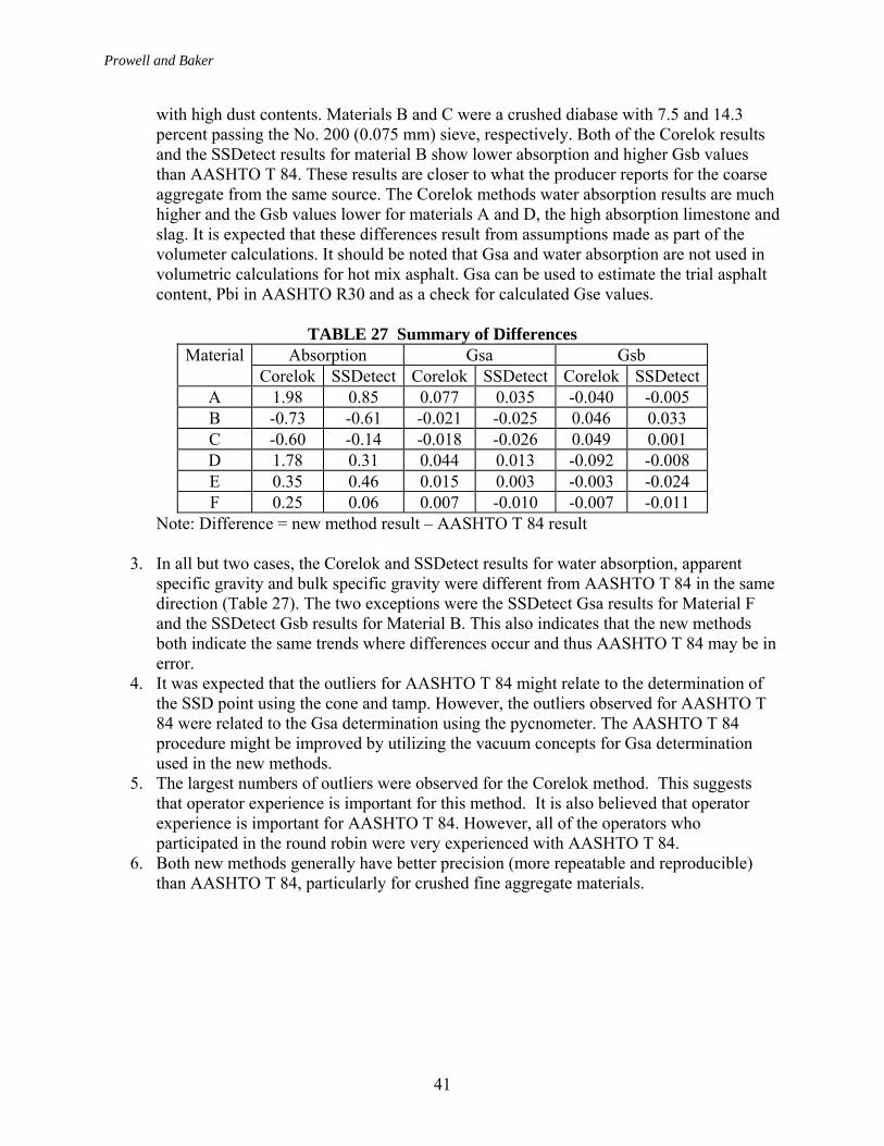
Prowell and Baker

41

with high dust contents. Materials B and C were a crushed diabase with 7.5 and 14.3 percent passing the No. 200 (0.075 mm) sieve, respectively. Both of the Corelok results and the SSDetect results for material B show lower absorption and higher Gsb values than AASHTO T 84. These results are closer to what the producer reports for the coarse aggregate from the same source. The Corelok methods water absorption results are much higher and the Gsb values lower for materials A and D, the high absorption limestone and slag. It is expected that these differences result from assumptions made as part of the volumeter calculations. It should be noted that Gsa and water absorption are not used in volumetric calculations for hot mix asphalt. Gsa can be used to estimate the trial asphalt content, Pbi in AASHTO R30 and as a check for calculated Gse values.

TABLE 27 Summary of Differences

Absorption Gsa Gsb Material Corelok SSDetect Corelok SSDetect Corelok SSDetect

A 1.98 0.85 0.077 0.035 -0.040 -0.005 B -0.73 -0.61 -0.021 -0.025 0.046 0.033 C -0.60 -0.14 -0.018 -0.026 0.049 0.001 D 1.78 0.31 0.044 0.013 -0.092 -0.008 E 0.35 0.46 0.015 0.003 -0.003 -0.024 F 0.25 0.06 0.007 -0.010 -0.007 -0.011

Note: Difference = new method result – AASHTO T 84 result

3. In all but two cases, the Corelok and SSDetect results for water absorption, apparent specific gravity and bulk specific gravity were different from AASHTO T 84 in the same direction (Table 27). The two exceptions were the SSDetect Gsa results for Material F and the SSDetect Gsb results for Material B. This also indicates that the new methods both indicate the same trends where differences occur and thus AASHTO T 84 may be in error.

4. It was expected that the outliers for AASHTO T 84 might relate to the determination of the SSD point using the cone and tamp. However, the outliers observed for AASHTO T 84 were related to the Gsa determination using the pycnometer. The AASHTO T 84 procedure might be improved by utilizing the vacuum concepts for Gsa determination used in the new methods.

5. The largest numbers of outliers were observed for the Corelok method. This suggests that operator experience is important for this method. It is also believed that operator experience is important for AASHTO T 84. However, all of the operators who participated in the round robin were very experienced with AASHTO T 84.

6. Both new methods generally have better precision (more repeatable and reproducible) than AASHTO T 84, particularly for crushed fine aggregate materials.

Prowell and Baker

42

RECOMMENDATIONS Based on the results of this study, it appears that the SSDetect method produced results that are close to AASHTO T 84 while offering time savings and improved precision. The SSDetect is recommended as an alternate to AASHTO T 84. The Corelok method produced results that were close to AASHTO T 84 for natural sands and most likely more accurate results for angular materials with high dust contents. However, caution is recommended when using the Corelok method on high absorption materials. The Corlok method also offers significant time savings and improved precision. Operator training would be important for the Corelok method. Based on Table 27, differences in measured Gsb, as high as 0.049, may occur between AASHTO T 84 and the new methods. As noted previously, the results from the new devices may actually be more accurate, or closer to the “true” value than those produced with AASHTO T 84. However, differences in the measured Gsb between the new methods and AASHTO T 84 will affect the VMA calculated for an HMA mix. Figure 7 illustrates the affect on calculated VMA resulting from a 0.040 difference in Gsb for varying percentages of fine aggregate in the blend. The assumptions used to produce the figure was a blend aggregate Gsb of 2.700, asphalt content of 5 percent, and compacted sample Gmb of 2.444. Based on Figure 7, if 30 percent of a fine aggregate were included in a blend, a difference in the measured Gsb of 0.040 would produce a difference in the calculated VMA of approximately 0.4 percent. It should also be noted that the 0.040 difference in Gsb is less than the within-lab d2s (expected difference between two test results) for AASHTO T 84 determined with the materials used in this study (0.049). The between-lab d2s for AASHTO T 84 determined in this study was 0.093. Therefore, the observed differences with the new measuring techniques were within the normal testing variability of AASHTO T 84.

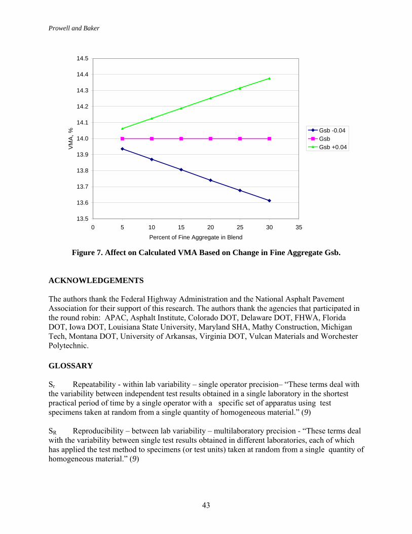
Prowell and Baker

43

13.5

13.6

13.7

13.8

13.9

14.0

14.1

14.2

14.3

14.4

14.5

0 5 10 15 20 25 30 35

Percent of Fine Aggregate in Blend

VMA

, %

Gsb -0.04GsbGsb +0.04

Figure 7. Affect on Calculated VMA Based on Change in Fine Aggregate Gsb.

ACKNOWLEDGEMENTS The authors thank the Federal Highway Administration and the National Asphalt Pavement Association for their support of this research. The authors thank the agencies that participated in the round robin: APAC, Asphalt Institute, Colorado DOT, Delaware DOT, FHWA, Florida DOT, Iowa DOT, Louisiana State University, Maryland SHA, Mathy Construction, Michigan Tech, Montana DOT, University of Arkansas, Virginia DOT, Vulcan Materials and Worchester Polytechnic. GLOSSARY Sr Repeatability - within lab variability – single operator precision– “These terms deal with the variability between independent test results obtained in a single laboratory in the shortest practical period of time by a single operator with a specific set of apparatus using test specimens taken at random from a single quantity of homogeneous material.” (9) SR Reproducibility – between lab variability – multilaboratory precision - “These terms deal with the variability between single test results obtained in different laboratories, each of which has applied the test method to specimens (or test units) taken at random from a single quantity of homogeneous material.” (9)

Prowell and Baker

44

d2s Acceptable range of more than two test results. “The range for different numbers of test results including two that would be equaled or exceeded in only 1 case in 20 is obtained by multiplying the appropriate standard deviation (1s) or coefficient of variation (1s%) by the appropriate factor.” (9) One case in 20 is equivalent to 95 percent confidence. The appropriate multiplier for two test results is 2.8 (more accurately 2√2). If the coefficient of variation is used, d2s is expressed as d2s% and then represents the percentage difference between two test results.

CV Coefficient of variation – standard deviation divided by the mean. ANOVA Analysis of Variance – a statistical technique for comparing the population means

between two or more populations. The t-test is limited to comparing two populations. Bias Bias is the difference between the measured result and the true value of the

measured property. Precision Precision is a measure of the variability of the test procedure and how repeatable

the test will be for a single operator or between different laboratories. F-test The one-tailed probability that the variances (standard deviation is the positive

square root of variance.) of two populations are significantly different (11). F-value A measurement of the distance between individual distributions used in ANOVA.

The F-value is calculated as the some of squares for a given factor divided by the sum of squares for error. The larger the F-value for a given factor compared to other factors in an experiment, the greater the effect that factor has. A larger F-value results in a smaller p-value (15).

GLM General Linear Model – a statistical means for conducting univariate and

multivariate analysis of variance with both balanced and unbalanced designs. Calculations are done using a regression approach (11).

h-statistic The h statistic is an indicator of how one laboratory’s average for a material

compares with the average of the other laboratories. The h statistic is based on Student’s t test (9).

k-statistic The k statistic is an indicator of how one laboratory’s variability for a given set of

replicate samples compares with that of all the other laboratories. The k statistic is based on the F ratio (9).

Replicate A test conducted on an independent sample of the same material using the same

operator, equipment and procedure in a relatively short time frame.

Prowell and Baker

45

REFERENCES

1. Standard Method of Test for Specific Gravity and Absorption of Fine Aggregates, American Association of State Highway and Transportation Officials, AASHTO Designation: T 84, 24th Edition, 2004.

2. American Society for Testing and Materials. 2005 ASTM Standards on Disk, Vol. 04.02, Concrete and Aggregates, ASTM International, Conshohocken, PA. 2005.

3. Dana, J.S. and R.J. Peters. Experimental Moisture Determination for Defining Saturated Surface Dry State of Highway Aggregates. Arizona Highway Department, Report No. 6, HPR 1-11 (153), June 1974.

4. Kandhal, P.S., Mallick, R.B., and Huner, M., “Development of a New Test Method for Measuring Bulk Specific Gravity of Fine Aggregates,” Transportation Research Record 1721, Transportation Research Board, National Academy of Sciences, Washington, DC, 2000, pp. 81-90.

5. Haddock, J.E. and Prowell, Brian D., “Determination of Aggregate Specific Gravity and Its Effect on HMA Mixture Performance,” Aggregate Contribution to Hot Mix Asphalt (HMA Performance, ASTM STP 1412, T. D. White, S. R. Johnson, and J. J. Yzenas, Eds. American Society for Testing Materials, West Conshohocken, PA, 2001.

6. Hall, Kevin D., “A Comparison of Fine Aggregate Specific Gravity Results and Variability Using Vacuum Sealing and SSD Methods,” Preprint, Transportation Research Board, National Academy of Sciences, Washington, DC, 2002.

7. Baker N “Developing Automated Methods for Determining Specific Gravity and Absorption of Fine Aggregates,” Masters Thesis, Auburn University, Auburn, AL, 2003.

8. Prowell, B. D. and N. V. Baker, “Development of a New Test Procedure for Determining the Bulk Specific Gravity of Fine Aggregates Using Automated Methods.” NCAT 02-13, National Center for Asphalt Technology, 2002.

9. American Society for Testing and Materials. ASTM Standards on Precision and Bias for Various Applications, ed 4. Philadelphia, 1992.

10. Personal communication with Kevin Hall. 11. Minitab Inc., Minitab Statistical Software, Version. 13.31, State College, PA. 2000. 12. Personal communication with Randy Weingart, Luck Stone Corporation. 13. American Society for Testing and Materials. Interlaboratory Data Analysis Software:

E 691 User’s Guide. Philadelphia, 1990. 14. Baker, N. V., B. D. Prowell and E. R. Brown. “Development of a New Test

Procedure for Determining the Bulk Specific Gravity of Fine Aggregate Using Automated Methods.” Transportation Research Record 1874, Transportation Research Board, Washington, D.C. 2004, pp. 11-18.

15. Six Sigma, “F-value ANOVA,” www.isixsigma.com/dictionary/F-value_ANOVA-248.htm, Accessed December 8, 2005.

Prowell and Baker

46

Appendix A

Ruggedness Study

Prowell and Baker

47

TABLE A-1 InstroTek Factors for Each Determination

TABLE A-2 Thermolyne Factors for Each Determination

1 2 3 4 5 6 7 8A 84 84 84 84 74 74 74 74

B 505 505 495 495 505 505 495 495

C 0.05 0 0.05 0 0.05 0 0.05 0

D 3 3 1 1 1 1 3 3

E 1005 995 1005 995 995 1005 995 1005

F 99 90 90 99 99 90 90 99

G 20 10 10 20 10 20 20 10

1 2 3 4 5 6 7 8A 84 84 84 84 74 74 74 74

B 505 505 495 495 505 505 495 495

C 0.05 0 0.05 0 0.05 0 0.05 0

D 3 3 1 1 1 1 3 3

E 1005 995 1005 995 995 1005 995 1005

F 99 90 90 99 99 90 90 99

G 20 10 10 20 10 20 20 10

FactorDetermination Number

Determination NumberReplicate Set Number 1

Factor

Replicate Set Number 2

1 2 3 4 5 6 7 8A 84 84 84 84 74 74 74 74

B 505 505 495 495 505 505 495 495

C 0.05 0 0.05 0 0.05 0 0.05 0

D 3 3 1 1 1 1 3 3

E 1005 995 1005 995 995 1005 995 1005

F 99 90 90 99 99 90 90 99

G 20 10 10 20 10 20 20 10

1 2 3 4 5 6 7 8A 84 84 84 84 74 74 74 74

B 505 505 495 495 505 505 495 495

C 0.05 0 0.05 0 0.05 0 0.05 0

D 3 3 1 1 1 1 3 3

E 1005 995 1005 995 995 1005 995 1005

F 99 90 90 99 99 90 90 99

G 20 10 10 20 10 20 20 10

FactorDetermination Number

Determination NumberReplicate Set Number 1

Factor

Replicate Set Number 2

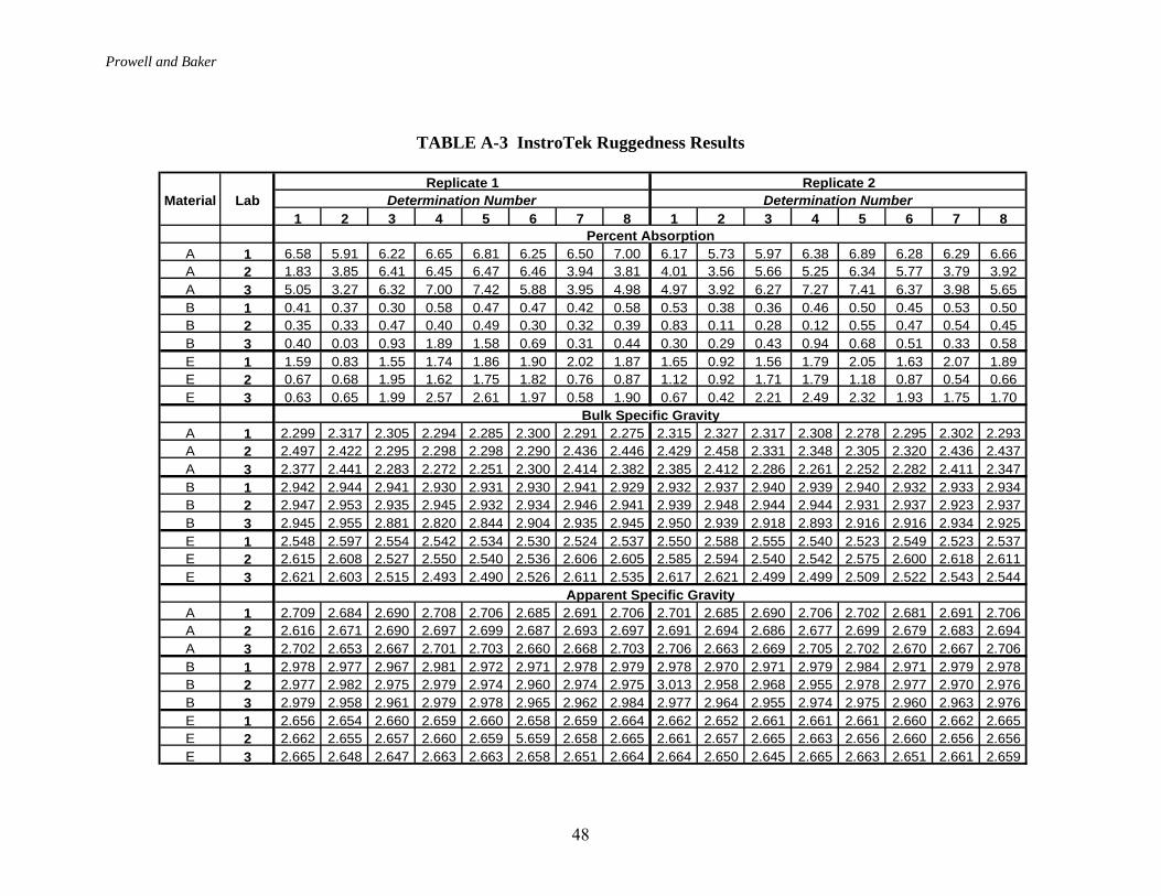
Prowell and Baker

48

TABLE A-3 InstroTek Ruggedness Results

1 2 3 4 5 6 7 8 1 2 3 4 5 6 7 8

A 1 6.58 5.91 6.22 6.65 6.81 6.25 6.50 7.00 6.17 5.73 5.97 6.38 6.89 6.28 6.29 6.66A 2 1.83 3.85 6.41 6.45 6.47 6.46 3.94 3.81 4.01 3.56 5.66 5.25 6.34 5.77 3.79 3.92A 3 5.05 3.27 6.32 7.00 7.42 5.88 3.95 4.98 4.97 3.92 6.27 7.27 7.41 6.37 3.98 5.65B 1 0.41 0.37 0.30 0.58 0.47 0.47 0.42 0.58 0.53 0.38 0.36 0.46 0.50 0.45 0.53 0.50B 2 0.35 0.33 0.47 0.40 0.49 0.30 0.32 0.39 0.83 0.11 0.28 0.12 0.55 0.47 0.54 0.45B 3 0.40 0.03 0.93 1.89 1.58 0.69 0.31 0.44 0.30 0.29 0.43 0.94 0.68 0.51 0.33 0.58E 1 1.59 0.83 1.55 1.74 1.86 1.90 2.02 1.87 1.65 0.92 1.56 1.79 2.05 1.63 2.07 1.89E 2 0.67 0.68 1.95 1.62 1.75 1.82 0.76 0.87 1.12 0.92 1.71 1.79 1.18 0.87 0.54 0.66E 3 0.63 0.65 1.99 2.57 2.61 1.97 0.58 1.90 0.67 0.42 2.21 2.49 2.32 1.93 1.75 1.70

A 1 2.299 2.317 2.305 2.294 2.285 2.300 2.291 2.275 2.315 2.327 2.317 2.308 2.278 2.295 2.302 2.293A 2 2.497 2.422 2.295 2.298 2.298 2.290 2.436 2.446 2.429 2.458 2.331 2.348 2.305 2.320 2.436 2.437A 3 2.377 2.441 2.283 2.272 2.251 2.300 2.414 2.382 2.385 2.412 2.286 2.261 2.252 2.282 2.411 2.347B 1 2.942 2.944 2.941 2.930 2.931 2.930 2.941 2.929 2.932 2.937 2.940 2.939 2.940 2.932 2.933 2.934B 2 2.947 2.953 2.935 2.945 2.932 2.934 2.946 2.941 2.939 2.948 2.944 2.944 2.931 2.937 2.923 2.937B 3 2.945 2.955 2.881 2.820 2.844 2.904 2.935 2.945 2.950 2.939 2.918 2.893 2.916 2.916 2.934 2.925E 1 2.548 2.597 2.554 2.542 2.534 2.530 2.524 2.537 2.550 2.588 2.555 2.540 2.523 2.549 2.523 2.537E 2 2.615 2.608 2.527 2.550 2.540 2.536 2.606 2.605 2.585 2.594 2.540 2.542 2.575 2.600 2.618 2.611E 3 2.621 2.603 2.515 2.493 2.490 2.526 2.611 2.535 2.617 2.621 2.499 2.499 2.509 2.522 2.543 2.544

A 1 2.709 2.684 2.690 2.708 2.706 2.685 2.691 2.706 2.701 2.685 2.690 2.706 2.702 2.681 2.691 2.706A 2 2.616 2.671 2.690 2.697 2.699 2.687 2.693 2.697 2.691 2.694 2.686 2.677 2.699 2.679 2.683 2.694A 3 2.702 2.653 2.667 2.701 2.703 2.660 2.668 2.703 2.706 2.663 2.669 2.705 2.702 2.670 2.667 2.706B 1 2.978 2.977 2.967 2.981 2.972 2.971 2.978 2.979 2.978 2.970 2.971 2.979 2.984 2.971 2.979 2.978B 2 2.977 2.982 2.975 2.979 2.974 2.960 2.974 2.975 3.013 2.958 2.968 2.955 2.978 2.977 2.970 2.976B 3 2.979 2.958 2.961 2.979 2.978 2.965 2.962 2.984 2.977 2.964 2.955 2.974 2.975 2.960 2.963 2.976E 1 2.656 2.654 2.660 2.659 2.660 2.658 2.659 2.664 2.662 2.652 2.661 2.661 2.661 2.660 2.662 2.665E 2 2.662 2.655 2.657 2.660 2.659 5.659 2.658 2.665 2.661 2.657 2.665 2.663 2.656 2.660 2.656 2.656E 3 2.665 2.648 2.647 2.663 2.663 2.658 2.651 2.664 2.664 2.650 2.645 2.665 2.663 2.651 2.661 2.659

Percent Absorption

Bulk Specific Gravity

Apparent Specific Gravity

Material LabReplicate 1 Replicate 2

Determination Number Determination Number

Prowell and Baker

49

TABLE A-4 Thermolyne Ruggedness Results

Replicate 1 Replicate 2 Determination Number Determination Number Material Lab

1 2 3 4 5 6 7 8 1 2 3 4 5 6 7 8 Percent Absorption A 1 4.44 6.34 5.46 5.94 4.96 4.92 4.32 6.76 6.62 4.68 3.62 5.30 3.86 4.48 5.28 5.52 A 2 5.16 4.28 4.48 6.06 6.58 6.20 5.12 5.34 6.36 4.36 5.34 6.14 4.88 5.92 5.70 4.96 A 3 6.20 5.42 3.16 4.82 0.541 4.00 4.20 4.52 4.70 3.82 4.10 6.94 3.40 4.64 5.36 4.66 B 1 1.02 1.02 0.82 1.22 0.84 0.78 0.64 0.76 0.60 0.68 0.84 1.02 0.94 1.06 0.62 0.72 B 2 0.92 0.80 0.76 1.08 1.08 0.70 0.88 0.84 1.06 0.74 1.04 1.28 1.02 1.18 0.94 0.98 E 1 2.28 2.18 2.02 2.78 2.54 3.00 3.22 2.76 2.34 2.62 2.30 2.90 1.84 2.46 2.32 2.64 E 2 NA NA NA NA NA NA NA NA NA NA NA NA NA NA NA NA Bulk Specific Gravity A 1 2.384 2.276 2.319 2.292 2.341 2.333 2.358 2.258 2.259 2.339 2.401 2.315 2.395 2.356 2.304 2.316A 2 2.344 2.385 2.389 2.301 2.262 2.294 2.333 2.346 2.282 2.382 2.338 2.296 2.355 2.301 2.308 2.366A 3 2.300 2.336 2.460 2.369 2.654 2.410 2.405 2.388 2.383 2.423 2.409 2.251 2.442 2.364 2.333 2.373B 1 2.879 2.881 2.895 2.868 2.904 2.902 2.924 2.909 2.925 2.913 2.902 2.890 2.894 2.884 2.916 2.917B 2 2.897 2.909 2.915 2.885 2.889 2.914 2.904 2.907 2.890 2.915 2.894 2.874 2.892 2.875 2.897 2.900E 1 2.501 2.509 2.517 2.470 2.487 2.452 2.435 2.470 2.498 2.482 2.499 2.463 2.527 2.490 2.504 2.485E 2 NA NA NA NA NA NA NA NA NA NA NA NA NA NA NA NA Apparent Specific Gravity A 1 2.667 2.660 2.655 2.654 2.649 2.636 2.626 2.666 2.657 2.627 2.629 2.639 2.639 2.634 2.623 2.655A 2 2.666 2.656 2.675 2.674 2.658 2.674 2.649 2.682 2.670 2.658 2.671 2.672 2.661 2.664 2.658 2.681A 3 2.442 2.462 2.537 2.483 2.640 2.507 2.506 2.496 2.494 2.515 2.507 2.408 2.525 2.474 2.458 2.484B 1 2.966 2.968 2.965 2.972 2.976 2.970 2.980 2.975 2.977 2.972 2.974 2.978 2.975 2.975 2.970 2.979B 2 2.976 2.978 2.981 2.978 2.982 2.974 2.980 2.980 2.982 2.980 2.984 2.983 2.980 2.976 2.978 2.985E 1 2.652 2.655 2.652 2.652 2.655 2.646 2.642 2.651 2.653 2.655 2.652 2.653 2.650 2.653 2.658 2.659E 2 NA NA NA NA NA NA NA NA NA NA NA NA NA NA NA NA

Note: NA = not available. 1Appears to be erroneous result.

Prowell and Baker

50

Appendix B

Corelok Test Method in AASHTO Forma

Prowell and Baker

51

(AASHTO Format) Standard Test Method for DETERMINING THE SPECIFIC GRAVITY AND ABSORPTION OF FINE AGGREGATES USING THE CORELOK

1. SCOPE 1.1 This method covers the determination of bulk and apparent specific gravity and

absorption of fine aggregates. 1.2 The values stated are in SI units. SI units are to be regarded as the

standard.

1.3 This standard may involve hazardous materials, operations, and equipment. This standard does not purport to address all of the safety problems associated with its use. It is the responsibility of whoever uses this standard to consult and establish appropriate safety and health practices and determine the applicability of regulatory limitations prior to use.

2. REFERENCED DOCUMENTS 2.1 AASHTO Standards

M 231 Weighing Devices Used in the Testing of Material R 1 Use of the International System of Units T 2 Sampling of Aggregates T 19 Bulk Density (“Unit Weight”) and Voids in Aggregate T 85 Specific Gravity and Absorption of Coarse Aggregate T 133 Density of Hydraulic Cement T 248 Reducing Samples of Aggregate to Testing Size T 255 Total Evaporable Moisture Content of Aggregate by Drying T 304 Uncompacted Void Content of Fine Aggregate

2.2 ASTM Standards

C 125 Terminology Relating to Concrete and Concrete Aggregates C 670 Practice and Preparing Precision and Bias Statements for Test

Methods for Construction Materials.

3. SIGNIFICANCE AND USE 3.1 Bulk specific gravity is the characteristic generally used for calculation of

the volume occupied by the aggregate in various mixtures containing aggregate including Portland cement concrete, bituminous concrete, and other mixtures that are proportioned or analyzed on an absolute volume basis. Bulk specific gravity is used in the computation of voids in aggregate in T 304 and T 19. Bulk specific gravity determined on the

Prowell and Baker

52

saturated surface dry basis is used if the aggregate is wet, that is, if its absorption has been satisfied. Conversely, the bulk specific gravity determined on the oven-dry basis is used for computations when the aggregate is dry or assumed to be dry.

3.2 Apparent specific gravity pertains to the relative density of the solid

material making up the constituent particles not including the pore space within the particles that is accessible to water.This value is not widely used in construction aggregate technology.

3.3 Water absorption values are used to calculate the change in the mass of an

aggregate due to water absorbed in the pore spaces within the constituent particles, compared to the dry condition, when it is deemed that the aggregate has been in contact with water long enough to satisfy most of the absorption potential. The laboratory standard for absorption is that obtained after submerging dry aggregate for approximately 15 hours in water. Aggregates mined from below the water table may have a higher absorption when used, if not allowed to dry. Conversely, some aggregates when used may contain an amount of absorbed moisture less than the 15 hours soaked condition: For an aggregate that has been in contact with water and that had free moisture on the particle surface, the percentage of free moisture can be determined by deducting the absorption from the total moisture content determined by T 255 by drying.

4. APPARATUS

4.1 Balance – conforming to the requirements of M 231, Class G 2.

4.2 Spray bottle – capable of producing a fine mist. 4.3 Isopropyl Alcohol 4.4 Beaker – capable of holding 1000 ml. 4.5 Volumeter – with the approximate dimensions: inside diameter of 137 mm

(5.375 in), wall thickness of 7 mm (0.275 in) and an overall height 108 mm (4.25 in).

4.6 Volumeter Clamping Apparatus – capable of securely holding the

volumeter and its lid. The apparatus shall apply enough pressure to the top of the lid to ensure metal on metal contact between the volumeter and its lid. The apparatus shall also consist of a level indicator that is securely fastened to the apparatus.

4.7 Aluminum spatula – approximately 230 mm (9 in) long, 25 mm (1 in)

wide and 3.2 mm (1/8) in thick with a straight edge for the end.

Prowell and Baker

53

4.8 Syringe - consisting of a 50 mm (2 in) needle and capable of holding 50

cc. 4.9 Corelok Device – consisting of a vacuum pump that is capable of reaching

667 Pa (5 mm Hg) in approximately 30 seconds. The chamber shall be flat with no curves or angles consisting inside dimensions of 425 x 184 x 498 mm (16.75 x 7.25 x 19.6”) (W x H x Depth). The device shall also consist of pressure induced sealing mechanism where sealing is induced by a bladder that provides enough pressure to ensure a proper sealing with wrinkles present in the plastic bag. The sealing bar shall be approximately 406 mm (16”) in length.

4.10 Plastic Bags – Bag shall be 292 mm (11.5”) wide, 356 mm (14”) long and

be 0.15 mm (0.006 in) in thickness. The bags shall be made of a material that is puncture resistant, flexible, impermeable to water, display no drifting during water displacement and should weigh within +/- 1 gram per sheet per roll.

4.11 Filler plates – 3 filler plates shall be placed in the chamber. The plates

should be made of a hard plastic with the dimensions of 410 x 380 x 20 mm (16 x 15 x 0.8 in) (L x W x Thickness).

4.12 Plastic coated sample holder – capable of supporting the sample under

water.

4.13 AggSpec software – version 02.08.13 or later.

4.14 I300 absolute vacuum gauge or similar device that is NIST traceable – consisting of a range of 0 – 5.33 kPa (0 – 40 mm Hg) with an accuracy of +/- 2% of full scale deflection at 20oC (68oF) with an operating temperature range from 10 to 50oC (50 to 122oF).

5. CALIBRATION 5.1 Calibration of the vacuum chamber should be conducted once a year. The

vacuum chamber should be calibrated with an I300 absolute vacuum or similar device that is NIST traceable.

5.2 Calibration of Volumeter

5.2.1 The calibration of the volumeter should be performed occasionally at the 23oC

test temperature. The equipment must be kept clean and free from any accumulations that would change the mass of the volumeter.

5.2.2 Immerse the volumeter and volumeter lid into a 23 +/- 1.7oC (73 +/- 3oF) water

bath for no less than 5 minutes.

Prowell and Baker

54

5.2.3 Remove the volumeter and volumeter lid from the water bath and dry with an

absorptive cloth.

5.2.4 Place the empty volumeter in the clamping fixture and push the bowl until it makes contact with the stops.

5.2.5 Fill the volumeter with 23 +/- 1.7oC (73 +/- 3oF) water to the level of the line

indicated inside the bowl (~ 6 mm (0.25 in) from the top).

5.2.6 Use a spray bottle and generously spray the top of the water with isopropyl (rubbing) alcohol to eliminate any air bubbles.

5.2.7 Place the lid on the volumeter with the small hole on the surface of the lid facing

to the front and close the clamps, make sure the lid and bowl make metal-to-metal contact.

5.2.8 Use the syringe to gently fill the bowl through the hole on top of the lid post until

water is seen coming out the hole on the surface of the lid. Wipe off excess water from the container and fixture with a towel.

5.2.9 Place the entire fixture with the volumeter on the scale and obtain the weight to

the nearest 0.1g.

5.2.10 Repeat the above steps for a total of 3 times and average the weights. Record the average weight in the worksheet.

6. SAMPLING 6.1 Sampling shall be accomplished in general accordance with T 2.

7. PREPARATION OF TEST SPECIMEN

7.1 Obtain approximately 2.5 kg of the fine aggregate from the sample using

the applicable procedures described in T 248.

7.2 Dry it in a suitable pan or vessel to constant mass at a temperature of 110 +/- 5oC (230 +/- 9oF). Allow it to cool to 23 +/- 1.7oC (73 +/- 3oF).

7.2.1 As an alternative, where the absorption and specific gravity values are to

be used in proportioning concrete mixtures with aggregate used in their naturally moist condition, the requirement for initial drying to constant mass may be eliminated.

7.3 Split the test sample according to T248 into one 1000 +/- 5g sample and

two 500 +/- 5g samples. Discard excess.

Prowell and Baker

55

8. PROCEDURE

8.1 Make and record all mass determinations to 0.1 g.

8.2 Insert all three filler plates into the chamber. 8.3 Bulk Determination

8.3.1 Weigh and record the dry sample weight of one of the 500 +/- 5g samples.

8.3.2 Place the volumeter and volumeter lid in a water bath at 23 +/- 1.7oC (73

+/- 3oF) for at least 5 minutes.

8.3.3 Dry the outside of the volumeter and volumeter lid. Place the empty volumeter in the clamping fixture and push the bowl until it makes contact with the stops. Place approximately 500 ml of 23 +/- 1.7oC (73 +/- 3oF) water in the volumeter.

Note 1 – This water should come from the water bath that the volumeter and volumeter lid was placed in (step 8.3.2).

8.3.4 Slowly and evenly distribute the sample into the volumeter. Once the

sample is placed in the volumeter, fill the container with 23 +/- 1.7oC (73 +/- 3oF) water to the line inside the container (~ 0.25” from the top). It is important to keep the water level at or below the line to avoid the loss of the fine aggregate during the lid placement.

8.3.5 Push the aluminum spatula to the bottom of the volumeter against the

inside circumference. Slowly and gently drag the spatula to the center of the bowl, removing the spatula after reaching the center. Repeat this same procedure 7 more times so that the entire circumference is covered in 8 equal angles (45 degrees until the starting point is reached).

8.3.6 Use a spray bottle and generously spray the top of the water with

isopropyl (rubbing) alcohol. This will immediately eliminate all surface air bubbles.

8.3.7 Place the lid on the volumeter with the small hole on the surface of the lid

facing to the front and lock the clamps. Use the syringe and fill the bowl through the hole on top of the lid post. Fill the volumeter until water comes out the 3.2 mm (1/8”) hole on the surface lid. Wipe the excess water from the container and fixture with a towel.

8.3.8 Determine the total mass of the volumeter, lid, water, sample and

clamping fixture to nearest 0.1g.

Prowell and Baker

56

8.3.9 Repeat steps 8.3.1 through 8.3.8 for the second 500 +/- 5g sample.

Note 2 -- The above steps (8.3.4-8.3.8) should be completed within 2 +/- 0.5 minutes.

8.4 Apparent Determination

8.4.1 Set the vacuum unit to a vacuum level of 99% and dwell time to a

minimum of 15 seconds. 8.4.2 Place all three spacer blocks into the vacuum chamber.

8.4.3 Obtain a plastic bag and record its mass to the nearest 0.1g.

8.4.4 Obtain the 1000 +/- 5 g sample and determine its dry mass.

8.4.5 Place the sample in the bag. Support the bottom of the bag on a tabletop

to protect against puncture and impact points. Place the bag containing the sample into the chamber. Fold the bag by approximately 25 mm (1”) at the opening. This will allow you to distribute the material inside the bag by gently shaking the bag side to side and not lose any material. Make certain that the material is as flat as possible inside the bag. Piling of the aggregate will restrict the airflow out of the sample.

Note 3 - Do not use your hand to squeeze the sample flat.

8.4.6 Place the open side of the bag over the seal bar and close the chamber

door. After the chamber door opens, gently remove the sample from the chamber.

8.4.7 Weighing in Water---Immediately immerse the vacuumed sample in a 23

+/- 1.7oC (73 +/- 3oF) water bath. Cut one corner of the bag, approximately 25 mm (1”) from the side. Make sure the bag is completely submerged before cutting (at least 51 mm (2”) from the top of the tank water level). Introducing air into the bag will produce inaccurate results.

8.4.8 Open the cut portion of the bag with your fingers and allow the water to

freely flow into the bag. Allow any small residual air bubbles to escape. Suspend the bag containing the sample over a holding basket connected to the scales. Make sure that the bag is not touching the sides or bottom of the water tank; allow the sample to stay immersed in the water bath for 10 +/- 1 minute.

8.4.9 Determine the submerged mass to the nearest 0.1g.

Prowell and Baker

57

Note 4 – Do not leave vacuumed sample outside the water for any reason. Immediately transfer the vacuumed sample to the water bath.

9. CALCULATIONS

9.1 Calculate the bulk and apparent specific gravity and the absorption by

entering data into the AggSpec software as follows:

9.1.1 Enter the average mass of the volumeter and clamping fixture filled with water (from step 5.2.10) into the space provided for fine aggregates at the top of the worksheet.

9.1.2 Enter the sample identification into the column labeled sample ID. 9.1.3 In the aggregate grade column, select fine for grade type.

9.1.4 Average the two dry masses from step 8.3.1 and enter the value into the

‘Dry Sample A Weight’ column.

9.1.5 Average the two masses from step 8.3.8 and enter the value into the ‘Sample A Weight in Container Filled With Water’ column.

9.1.6 Input the bag weight (8.4.3) into the column labeled ‘Bag Weight’.

9.1.7 Input the dry sample mass for the apparent determination (8.4.4) into the

column labeled ‘Dry Sample B Weight’.

9.1.8 Enter the submerged mass (8.4.9) into the column labeled ‘Weight of Sealed Sample B Opened in Water’.

9.1.9 The equations used to calculate the bulk specific gravity, apparent specific

gravity and absorption can be found in Appendix A. 10. REPORT 10.1 Report the specific gravity results to the nearest 0.001 and absorption to the nearest 0.01 percent. 11. APPENDIX A – Equations Used in the CoreLok System for

Determination of Absorption, Apparent Gravity and Bulk Gravity of Aggregates

Prowell and Baker

58

This section provides details on the equations used in the CoreLok method. We start by defining the following:

a = Fractional absorption

ρv = Apparent specific gravity ρu = Apparent bulk specific gravity Va = Volume of sample, including the pores Vabs = Volume of pores Ma = Mass of sample ρw = Density of water

In this method two densities are measured, one fully saturated using the CoreLok, ρv, and the other “unsaturated” using a calibrated volumeter, ρu. With these two densities measured, one can derive the following relations.

VaMa

u =ρ (1)

absV VVa

Ma−

=ρ (2)

Wabs

MaaVρ

= (3)

Substituting equation (3) in equation (2) and rearranging

WuW

V aaMaVa

ρρρ

ρ−

=−

=1

11 (4)

Rearranging equation (4) and solving for absorption,

WuV

uVa ρρρρρ

⎟⎟⎠

⎞⎜⎜⎝

⎛ −= (5)

Obviously percent absorption is 100 multiplied by a. Notice, the apparent bulk specific gravity (the unsaturated density), ρu, is determined using a calibrated volumeter. It is recommended that this measurement be completed in less then 2 minutes. The reason for this short test time is to make certain that no absorption is taking place during this time. However, realistically, the amount of water absorbed by the aggregates varies during the two minutes depending on a

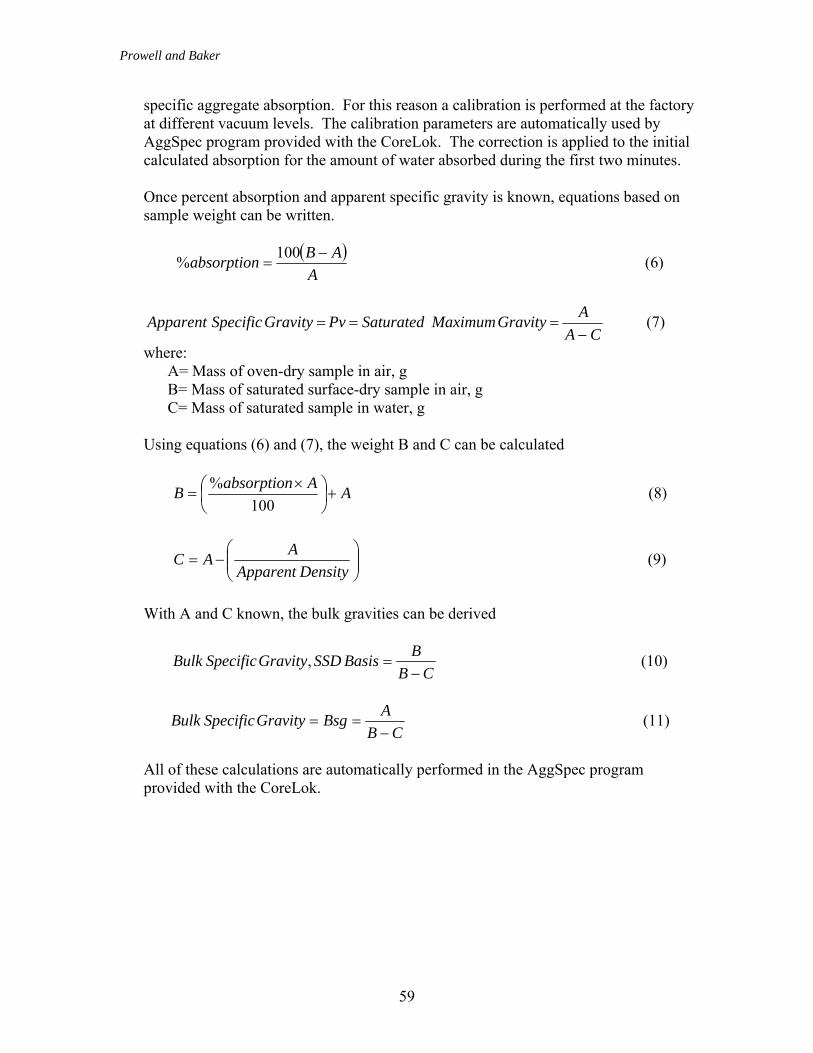
Prowell and Baker

59

specific aggregate absorption. For this reason a calibration is performed at the factory at different vacuum levels. The calibration parameters are automatically used by AggSpec program provided with the CoreLok. The correction is applied to the initial calculated absorption for the amount of water absorbed during the first two minutes. Once percent absorption and apparent specific gravity is known, equations based on sample weight can be written.

( )A

ABabsorption −=

100% (6)

CAAGravityMaximumSaturatedPvGravitySpecificApparent−

=== (7)

where: A= Mass of oven-dry sample in air, g

B= Mass of saturated surface-dry sample in air, g C= Mass of saturated sample in water, g Using equations (6) and (7), the weight B and C can be calculated

AAabsorptionB +⎟⎠⎞

⎜⎝⎛ ×

=100

% (8)

⎟⎟⎠

⎞⎜⎜⎝

⎛−=

DensityApparentAAC (9)

With A and C known, the bulk gravities can be derived

CBBBasisSSDGravitySpecificBulk−

=, (10)

CBABsgGravitySpecificBulk−

== (11)

All of these calculations are automatically performed in the AggSpec program provided with the CoreLok.

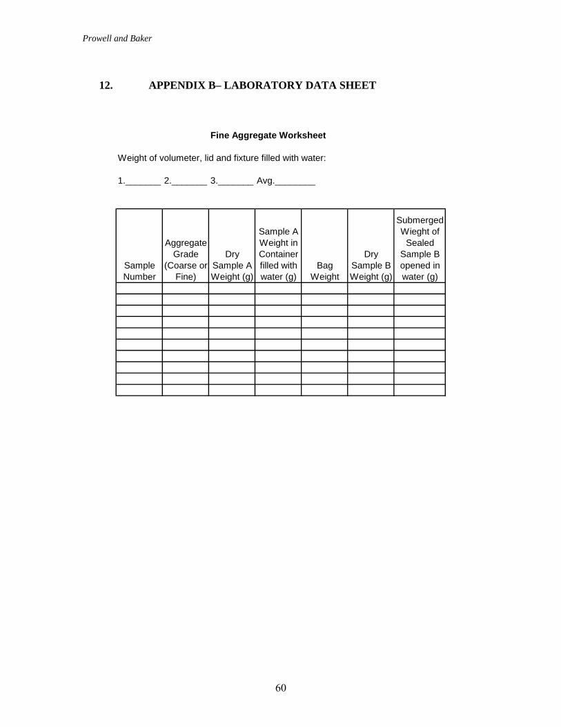
Prowell and Baker

60

12. APPENDIX B– LABORATORY DATA SHEET

Fine Aggregate Worksheet

Weight of volumeter, lid and fixture filled with water:

1._______ 2._______ 3._______ Avg.________

Sample Number

Aggregate Grade

(Coarse or Fine)

Dry Sample A Weight (g)

Sample A Weight in Container filled with water (g)

Bag Weight

Dry Sample B Weight (g)

Submerged Wieght of

Sealed Sample B opened in water (g)

Prowell and Baker

61

Appendix C

SSDetect Test Method in AASHTO Format

Prowell and Baker

62

(DRAFT AASHTO Format) Standard Test Method for DETERMINING THE SPECIFIC GRAVITY AND ABSORPTION OF FINE AGGREGATES USING THE SSDETECT

1. SCOPE 1.1 This method covers the determination of bulk and apparent specific

gravity and absorption of fine aggregates. 1.2 The values stated are in SI units. SI units are to be regarded as the

standard.

1.3 This standard may involve hazardous materials, operations, and equipment. This standard does not purport to address all of the safety problems associated with its use. It is the responsibility of whoever uses this standard to consult and establish appropriate safety and health practices and determine the applicability of regulatory limitations prior to use.

2. REFERENCED DOCUMENTS 2.1 AASHTO Standards

M 231 Weighing Devices Used in the Testing of Material R 1 Use of the International System of Units T 2 Sampling of Aggregates T 19 Bulk Density (“Unit Weight”) and Voids in Aggregate T 85 Specific Gravity and Absorption of Coarse Aggregate T 133 Density of Hydraulic Cement T 248 Reducing Samples of Aggregate to Testing Size T 255 Total Evaporable Moisture Content of Aggregate by Drying T 304 Uncompacted Void Content of Fine Aggregate

2.2 ASTM Standards

C 125 Terminology Relating to Concrete and Concrete Aggregates C 670 Practice and Preparing Precision and Bias Statements for Test

Methods for Construction Materials.

2.3 SSDetect Operational Instructions

3. SIGNIFICANCE AND USE

3.1 Bulk specific gravity is the characteristic generally used for calculation of the volume occupied by the aggregate in various mixtures containing

Prowell and Baker

63

aggregate including Portland cement concrete, bituminous concrete, and other mixtures that are proportioned or analyzed on an absolute volume basis. Bulk specific gravity is used in the computation of voids in aggregate in T 304 and T 19. Bulk specific gravity determined on the saturated surface dry basis is used if the aggregate is wet, that is, if its absorption has been satisfied. Conversely, the bulk specific gravity determined on the oven-dry basis is used for computations when the aggregate is dry or assumed to be dry.

3.2 Apparent specific gravity pertains to the relative density of the solid

material making up the constituent particles not including the pore space within the particles that is accessible to water. This value is not widely used in construction aggregate technology.

3.3 Water absorption values are used to calculate the change in the mass of an

aggregate due to water absorbed in the pore spaces within the constituent particles, compared to the dry condition, when it is deemed that the aggregate has been in contact with water long enough to satisfy most of the absorption potential. The laboratory standard for absorption is that obtained after submerging dry aggregate for approximately 15 hours in water. Aggregates mined from below the water table may have a higher absorption when used, if not allowed to dry. Conversely, some aggregates when used may contain an amount of absorbed moisture less than the 15 hours soaked condition: For an aggregate that has been in contact with water and that had free moisture on the particle surface, the percentage of free moisture can be determined by deducting the absorption from the total moisture content determined according to T 255 by drying.

4. APPARATUS

4.1 Balance – conforming to the requirements of M 231, Class G 2.

4.2 Large Neck Volumetric Flask – with a capacity of 500 mL. (Barnstead

Thermolyne Part # HRX36 has been found to be acceptable.) 4.3 Timer – capable of at least 5 minutes. 4.4 AVM Unit – The unit shall be an automated process for removing

entrapped air. It shall consist of the following devices: an orbiting mixer that can securely hold a 500 mL large neck volumetric flask, a clamp and clamping rod capable of holding the neck of the volumetric flask, a vacuum pump, hose, and a stopper capable of fitting the mouth of the volumetric flask.

4.5 SSDetect Device – The device shall be automatically capable of detecting

SSD using an infrared laserssource. It shall consist of an orbital mixer,

Prowell and Baker

64

water pump, infrared lasersource, infrared detector, and a mixing bowl with a lid. The lid of the mixing bowl shall consist of two sapphire lenses and contain an injection nozzle for water injection.

4.6 Distilled Water

5. CALIBRATION 5.1 Calibration of the pump and the SSDetect Unit shall be performed once a

month.

5.2 Calibration of Pump

5.2.1 Fill the SSDetect water reservoir to the bottom of the rubber gasket with distilled water and attach the cover.

5.2.2 Turn on the power switch on the rear of the SSDetect unit.

5.2.3 Immediately when the display illuminates, immediately press the center of

the SSDetect touch screen to go to the Manual Controls screen.

5.2.4 Press the right arrow key to advance to the Pump Calibration screen and press the enter key.

5.2.5 Place a clean, pre-weighed container under the nozzle in the lid to collect

the water. Position the container so as to minimize splashing.

Note 1 – An 125 mL Erlenmeyer flask or similar container is recommended

5.2.6 Press the start key to begin the water collection cycle. The pump will

inject 3000 times.

5.2.7 At the end of the collection cycle, remove the container and place it on a scale to obtain the total weight. Subtract the empty container weight obtained in step 5.2.5 from this value and enter the resulting amount as directed on the touch screen, using the up and down arrow keys. Press the exit key to end the calibration.

5.3 Calibration of SSDetect Unit 5.3.1 Check and ensure that the water reservoir is full on the SSDetect Unit.

Turn the unit on using the power switch in the rear of the device and allow the unit to complete the System Warm Up cycle (30 minutes).

Prowell and Baker

65

5.3.2 Once the warm up cycle has completed, turn off the power switch on the rear of the unit, wait for a couple of seconds and then turn the unit back on.

5.3.3 Immediately once the display illuminates, immediately press the center of

the SSDetect touch screen to go to the Manual Controls screen.

5.3.4 Press the right arrow key to advance to the SSDetect Unit Calibration screen and press the enter key.

5.3.5 Insert exactly 500.0 grams of calibration material provided by Barnstead

International into the mixing bowl and press start. After the unit completes the calibration procedure, the screen will display the calibration result.

5.3.6 Press OK to return back to the SSDetect Unit Calibration screen.

5.3.7 Press the right arrow to advance to the Exit screen and press enter to begin

testing.

5.3.8 Dry the calibration material back to a constant mass at a temperature of 110 +/- 5oC (230 +/- 9oF), so it can be used for future calibrations.

Note 2 – For more calibration material contact Barnstead Thermolyne or

obtain a sufficient amount of Ottawa Sand.

6. SAMPLING 6.1 Sampling shall be accomplished in general accordance with T 2. 7. PREPARATION OF TEST SPECIMEN

7.1 Obtain approximately 1 kg of the fine aggregate from the sample using the

applicable procedures described in T 248.

7.2 Dry it in a suitable pan or vessel to constant mass at a temperature of 110 +/- 5oC (230 +/- 9oF). Allow it to cool to 23 +/- 1.7oC (73 +/- 3oF).

7.3 Split the test sample according to T248 into two 500 +/- 5g samples.

Discard excess.

8. PROCEDURE

8.1 Make and record all mass determinations to 0.1 g. 8.2 Determine the mass of the volumetric flask filled to its calibration capacity

with water at 23 +/- 1.7oC (73 +/- 3oF).

Prowell and Baker

66

8.3 Film Coefficient and Apparent Specific Gravity Determination

8.3.1 Place approximately 250 mL of 23 +/- 1.7oC (73 +/- 3oF) water in a 500

mL large neck volumetric flask. 8.3.2 Place the flask that contains the water on a balance and zero the balance.

8.3.3 Set the timer to five minutes and start it.

8.3.4 Weigh out 500.0 grams +/- 0.1 gram, of aggregate and record the weight

to the nearest tenth of a gram. Transfer all of the aggregate into a flask. After recording the weight, make certain that the aggregate in the flask is covered with water. A small amount of water can be added at this time to rinse the sides of the flask if necessary. Make certain NOT to overfill the flask past the calibration mark. Keep the water level well below the calibration line.

Note 3 – A funnel may be used to help transfer the sample into the flask.

4.14.1 After the 5 minutes on the timer has elapsed, fill the flask with 23 +/-

1.7oC (73 +/- 3oF) water to the calibration mark.

8.3.5 Add a few drops of isopropyl alcohol or use a paper towel to remove bubbles if necessary to reduce error in reading the meniscus.

Note 4 – An accurate meniscus determination is very important.

8.3.6 After the 5 minutes on the timer has elapsed, fill the flask with 23 +/-

1.7oC (73 +/- 3oF) water to the calibration mark.

8.3.7 Weigh and record the weight of the flask with its contents.

8.3.8 Place the flask containing the sample in the mounting bracket on top of mixer of AVM unit. Tighten the clamp around the top portion of flask using the thumbscrew found on the clamp and then insert the rubber stopper, with vacuum hose attached, into flask.

8.3.9 Turn power switch, found on the rear of AVM unit, to the “on” position.

Press the “start” button on top of AVM unit to begin test. Mixer will begin to agitate material in flask, after several minutes the vacuum will turn on and begin to remove air from the sample. This operation is entirely automated. The unit will stop automatically when testing is complete. (~ 11 minutes) (Pat could you describe the automated shake times, vacuum times and vacuum levels) ). The mixer will operate for three minutes, then the vacuum pump will engage at a level of about 22”Hg for another three

Prowell and Baker

67

minutes. The last five minutes of the test the vacuum pump will engage at a level of about 27”Hg. The AVM will continue mixing during the entire period.

8.3.10 After the unit has stopped mixing, remove the flask from mixing platform.

Add a few drops of isopropyl alcohol or use a paper towel to remove bubbles if necessary to reduce error in reading the meniscus.

8.3.11 Fill the flask to the calibration mark.

8.3.12 Determine the total mass of the flask with the sample and water filled to

the calibration mark to nearest 0.1g.

8.3.13 Subtract the weight in step 8.3.7 from the weight in step 8.3.12. Enter this value into the following equation to determine the Film Coefficient.

Film Coefficient = 52 + (4 * X) – (0.11 * X2) where: X = the difference between steps 8.3.7 and 8.3.12, g.

8.4 Bulk Specific Gravity and Percent Absorption Determination

8.4.1 Turn the SSDetect device on and allow it to complete the 30 minute warm

up period.

8.4.2 Place the empty, clean and completely dry bowl from SSDetect on balance and record the weight of the bowl.

8.4.3 Place 500 +/- 0.1 grams of the sample into the bowl and record the weight

of the bowl and sample.

8.4.4 Calculate and record the dry aggregate weight by subtracting the weight in step 8.4.2 from 8.4.3.

8.4.5 Place the bowl with the aggregate into SSDetect device, making certain

that the notch in the front of the bowl fully engages in the notch in the front of the metal mounting plate. (Feel this with your finger at the bottom front of the bowl as placed.) Use the ring on the bowl to securely fasten the bowl to the plate by pressing down and turning the ring ¼ turn until tight. Next, place the top on the bowl and lightly press down to be certain it is engaged. The notch should be lined up in the front of the bowl. Then, close the lid to the SSDetect and latch in the front.

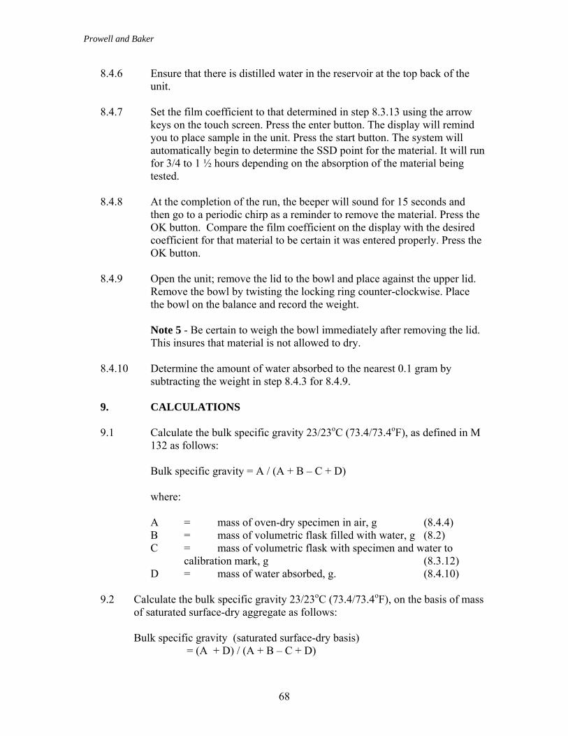
Prowell and Baker

68

8.4.6 Ensure that there is distilled water in the reservoir at the top back of the unit.

8.4.7 Set the film coefficient to that determined in step 8.3.13 using the arrow

keys on the touch screen. Press the enter button. The display will remind you to place sample in the unit. Press the start button. The system will automatically begin to determine the SSD point for the material. It will run for 3/4 to 1 ½ hours depending on the absorption of the material being tested.

8.4.8 At the completion of the run, the beeper will sound for 15 seconds and

then go to a periodic chirp as a reminder to remove the material. Press the OK button. Compare the film coefficient on the display with the desired coefficient for that material to be certain it was entered properly. Press the OK button.

8.4.9 Open the unit; remove the lid to the bowl and place against the upper lid.

Remove the bowl by twisting the locking ring counter-clockwise. Place the bowl on the balance and record the weight.

Note 5 - Be certain to weigh the bowl immediately after removing the lid. This insures that material is not allowed to dry.

8.4.10 Determine the amount of water absorbed to the nearest 0.1 gram by

subtracting the weight in step 8.4.3 for 8.4.9.

9. CALCULATIONS

9.1 Calculate the bulk specific gravity 23/23oC (73.4/73.4oF), as defined in M 132 as follows:

Bulk specific gravity = A / (A + B – C + D)

where: A = mass of oven-dry specimen in air, g (8.4.4) B = mass of volumetric flask filled with water, g (8.2)

C = mass of volumetric flask with specimen and water to calibration mark, g (8.3.12)

D = mass of water absorbed, g. (8.4.10)

9.2 Calculate the bulk specific gravity 23/23oC (73.4/73.4oF), on the basis of mass of saturated surface-dry aggregate as follows:

Bulk specific gravity (saturated surface-dry basis)

= (A + D) / (A + B – C + D)

Prowell and Baker

69

9.3 Calculate the apparent specific gravity 23/23oC (73.4/73.4oF), as defined in M

132 as follows: Apparent specific gravity = E / (E + B – C)

where: E = mass of oven-dry apparent specimen in air, g. (8.3.4) 9.4 Calculate the percentage absorption, as defined in ASTM C 125, as follows:

Water Absorption, percent = (D / A) X 100

10. REPORT 10.1 Report the specific gravity results to the nearest 0.001 and absorption to

the nearest 0.01 percent.

Prowell and Baker

70

11. APPENDIX A– LABORATORY DATA SHEET

Film Coefficient and Apparent Determination Bulk Gravity and Absorption Determination

E C X 1 2 A 3 D

Sample Number

Mass of Dry Aggregate,

g (8.3.4)

Initial Wt. of Flask w/

Contents, g (8.3.7)

Final Wt. of Flask w/

Contents, g (8.3.12)

X = Final - Initial Wt. Of Flask with

Contents, g

Film Coefficient

(8.3.13) = 52 + (4*X)-

(0.11*X^2) Bowl Wt., g (8.4.2)

Bowl + Dry Sample Wt.,

g (8.4.3)

Dry Sample Wt., g = (2) - (1) (8.4.4)

Bowl + SSD

Sample Wt., g (8.4.9)

Mass of water

Absorbed, g = (3) - (2)

Bulk Specific Gravity = A/(A+B-C+D)

Bulk Specific Gravity (SSD Basis) = (A+D)/(A+B-C+D)

Apparent Specific Gravity = E/(E+B-C)

Water Absorption, % = (D/A) x 100

B = Mass of Volumetric Flask, Filled with Water, g (8.2) =

Prowell and Baker

71

Appendix D

Round Robin Results

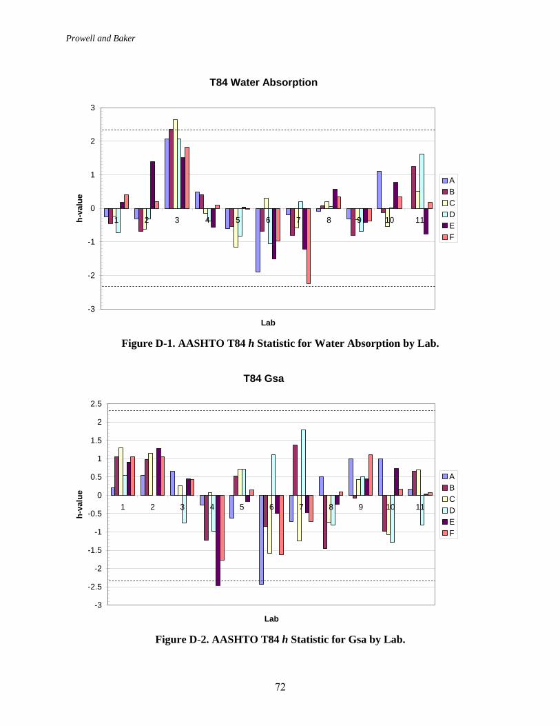
Prowell and Baker

72

T84 Water Absorption

-3

-2

-1

0

1

2

3

1 2 3 4 5 6 7 8 9 10 11

Lab

h-va

lue

ABCDEF

Figure D-1. AASHTO T84 h Statistic for Water Absorption by Lab.

T84 Gsa

-3

-2.5

-2

-1.5

-1

-0.5

0

0.5

1

1.5

2

2.5

1 2 3 4 5 6 7 8 9 10 11

Lab

h-va

lue

ABCDEF

Figure D-2. AASHTO T84 h Statistic for Gsa by Lab.

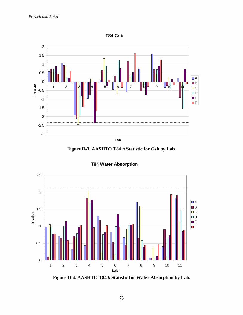
Prowell and Baker

73

T84 Gsb

-3

-2.5

-2

-1.5

-1

-0.5

0

0.5

1

1.5

2

1 2 3 4 5 6 7 8 9 10 11

Lab

h-va

lue

ABCDEF

Figure D-3. AASHTO T84 h Statistic for Gsb by Lab.

T84 Water Absorption

0

0.5

1

1.5

2

2.5

1 2 3 4 5 6 7 8 9 10 11Lab

k-va

lue

ABCDEF

Figure D-4. AASHTO T84 k Statistic for Water Absorption by Lab.

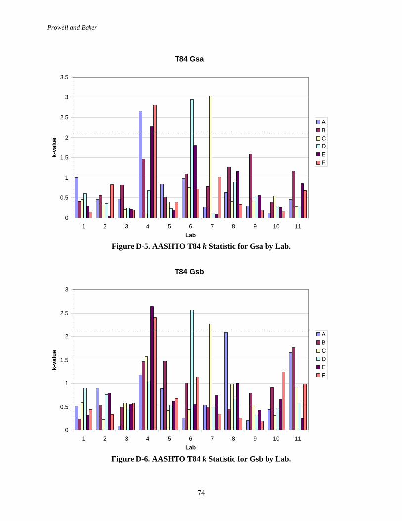
Prowell and Baker

74

T84 Gsa

0

0.5

1

1.5

2

2.5

3

3.5

1 2 3 4 5 6 7 8 9 10 11Lab

k-va

lue

ABCDEF

Figure D-5. AASHTO T84 k Statistic for Gsa by Lab.

T84 Gsb

0

0.5

1

1.5

2

2.5

3

1 2 3 4 5 6 7 8 9 10 11Lab

k-va

lue

ABCDEF

Figure D-6. AASHTO T84 k Statistic for Gsb by Lab.

Prowell and Baker

75

Corelok Water Absorption

-2

-1.5

-1

-0.5

0

0.5

1

1.5

2

2.5

3

1 2 3 4 5 6 7 8 9 10

Lab

h-va

lue

ABCDEF

Figure D-7. Corelok h Statistic for Water Absorption by Lab.

Corelok Gsa

-3

-2

-1

0

1

2

3

1 2 3 4 5 6 7 8 9 10

Lab

h-va

lue

ABCDEF

Figure D-8. Corelok h Statistic for Gsa by Lab.

Prowell and Baker

76

Corelok Gsb

-3

-2.5

-2

-1.5

-1

-0.5

0

0.5

1

1.5

2

1 2 3 4 5 6 7 8 9 10

Lab

h-va

lue

ABCDEF

Figure D-9. Corelok h Statistic for Gsb by Lab.

Corelok Water Absorption

0

0.5

1

1.5

2

2.5

3

3.5

1 2 3 4 5 6 7 8 9 10Lab

k-va

lue

ABCDEF

Figure D-10. Corelok k Statistics for Absorption by Lab.

Prowell and Baker

77

Corelok Gsa

0

0.5

1

1.5

2

2.5

3

3.5

1 2 3 4 5 6 7 8 9 10Lab

k-va

lue

ABCDEF

Figure D-11. Corelok k Statistics for Gsa by Lab.

Corelok Gsb

0

0.5

1

1.5

2

2.5

3

1 2 3 4 5 6 7 8 9 10Lab

k-va

lue

ABCDEF

Figure D-12. Corelok k Statistics for Gsb by Lab.

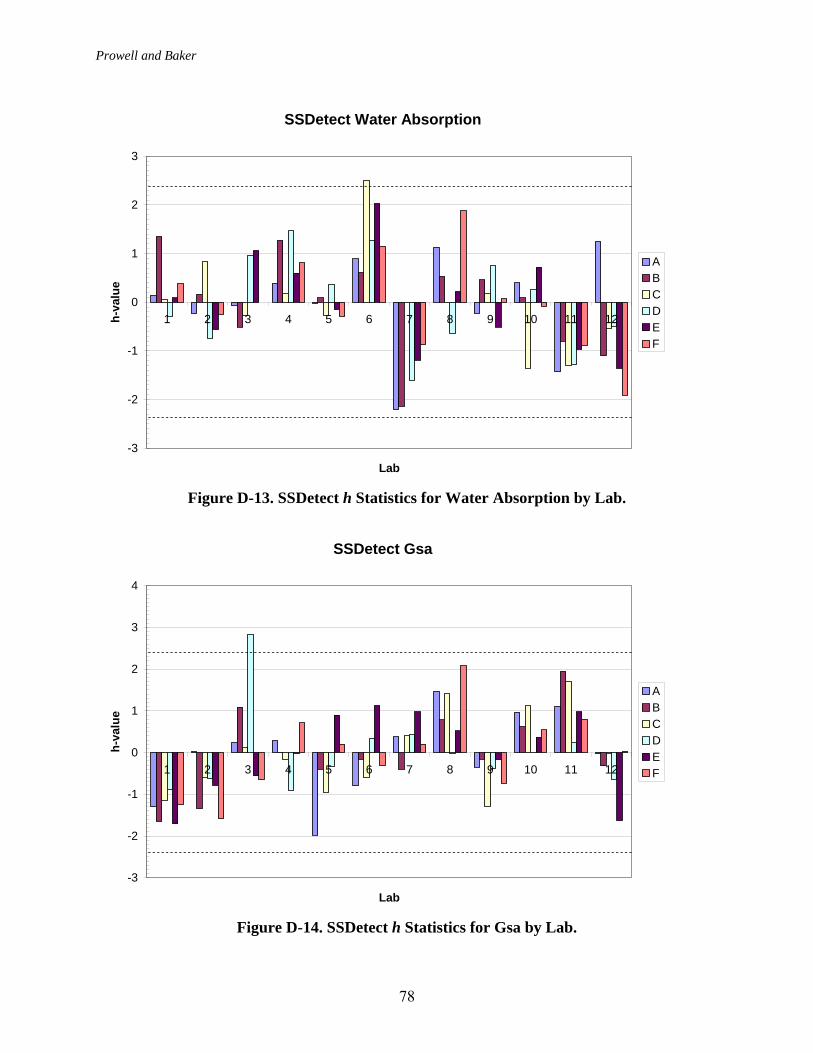
Prowell and Baker

78

SSDetect Water Absorption

-3

-2

-1

0

1

2

3

1 2 3 4 5 6 7 8 9 10 11 12

Lab

h-va

lue

ABCDEF

Figure D-13. SSDetect h Statistics for Water Absorption by Lab.

SSDetect Gsa

-3

-2

-1

0

1

2

3

4

1 2 3 4 5 6 7 8 9 10 11 12

Lab

h-va

lue

ABCDEF

Figure D-14. SSDetect h Statistics for Gsa by Lab.

Prowell and Baker

79

SSDetect Gsb

-2.5

-2

-1.5

-1

-0.5

0

0.5

1

1.5

2

2.5

1 2 3 4 5 6 7 8 9 10 11 12

Lab

h-va

lue

ABCDEF

Figure D-15. SSDetect h Statistics for Gsb by Lab.

SSDetect Water Absorption

0

0.5

1

1.5

2

2.5

3

1 2 3 4 5 6 7 8 9 10 11 12Lab

k-va

lue

ABCDEF

Figure D-16. SSDetect k Statistics for Absorption by Lab.

Prowell and Baker

80

SSDetect Gsa

0

0.5

1

1.5

2

2.5

3

3.5

1 2 3 4 5 6 7 8 9 10 11 12Lab

k-va

lue

ABCDEF

Figure D-17. SSDetect k Statistics for Gsa by Lab.

SSDetect Gsb

0

0.5

1

1.5

2

2.5

3

1 2 3 4 5 6 7 8 9 10 11 12Lab

k-va

lue

ABCDEF

Figure D-18. SSDetect k Statistics for Gsb by Lab.