rounding-based moves for metric labeling - m. pawan...
TRANSCRIPT

Rounding-based Moves for Metric Labeling
M. Pawan KumarEcole Centrale Paris & INRIA Saclay
Abstract
Metric labeling is a special case of energy minimization for pairwise Markov ran-dom fields. The energy function consists of arbitrary unary potentials, and pair-wise potentials that are proportional to a given metric distance function over thelabel set. Popular methods for solving metric labeling include (i) move-makingalgorithms, which iteratively solve a minimum st-cut problem; and (ii) the linearprogramming (LP) relaxation based approach. In order to convert the fractionalsolution of the LP relaxation to an integer solution, several randomized round-ing procedures have been developed in the literature. We consider a large classof parallel rounding procedures, and design move-making algorithms that closelymimic them. We prove that the multiplicative bound of a move-making algorithmexactly matches the approximation factor of the corresponding rounding proce-dure for any arbitrary distance function. Our analysis includes all known resultsfor move-making algorithms as special cases.
1 Introduction
A Markov random field (MRF) is a graph whose vertices are random variables, and whose edgesspecify a neighborhood over the random variables. Each random variable can be assigned a valuefrom a set of labels, resulting in a labeling of the MRF. The putative labelings of an MRF arequantitatively distinguished from each other by an energy function, which is the sum of potentialfunctions that depend on the cliques of the graph. An important optimization problem associate withthe MRF framework is energy minimization, that is, finding a labeling with the minimum energy.
Metric labeling is a special case of energy minimization, which models several useful low-levelvision tasks [3, 4, 21]. It is characterized by a finite, discrete label set and a metric distance functionover the labels. The energy function in metric labeling consists of arbitrary unary potentials andpairwise potentials that are proportional to the distance between the labels assigned to them. Theproblem is known to be NP-hard [23]. Two popular approaches for metric labeling are: (i) move-making algorithms [4, 9, 15, 16, 24], which iteratively improve the labeling by solving a minimumst-cut problem; and (ii) linear programming (LP) relaxation [5, 14, 20, 25], which is obtained bydropping the integral constraints in the corresponding integer programming formulation. Move-making algorithms are very efficient due to the availability of fast minimum st-cut solvers [2] and arevery popular in the computer vision community. In contrast, the LP relaxation is significantly slower,despite the development of specialized solvers [8, 10, 12, 13, 19, 22, 25, 26, 27, 28]. However, whenused in conjunction with randomized rounding algorithms, the LP relaxation provides the best knownpolynomial-time theoretical guarantees for metric labeling [1, 5, 11].
At first sight, the difference between move-making algorithms and the LP relaxation appears to bethe standard accuracy vs. speed trade-off. However, for some special cases of distance functions,it has been shown that appropriately designed move-making algorithms can match the theoreticalguarantees of the LP relaxation [15, 16, 23]. In this paper, we extend this result for a large class ofrandomized rounding procedures, which we call parallel rounding. In particular we prove that forany arbitrary (semi-)metric distance function, there exist move-making algorithms that match thetheoretical guarantees provided by parallel rounding. Our proofs are constructive, which allows usto test the rounding-based move-making algorithms empirically. Our experimental results are along
1
the same lines as those that were previously reported for various special distance functions [15, 16].Specifically, they confirm that rounding-based moves provide similar accuracy to the LP relaxationwhile being significantly faster.
2 Preliminaries
Metric Labeling. The problem of metric labeling is defined over an undirected graph G =(X,E). The vertices X = {X1, X2, · · · , Xn} are random variables, and the edges E specify aneighborhood relationship over the random variables. Each random variable can be assigned a valuefrom the label set L = {l1, l2, · · · , lh}. We assume that we are also provided with a metric distancefunction d : L × L → R
+ over the labels. Recall that a metric distance function satisfies the fol-lowing properties: (i) d(li, lj) ≥ 0 for all li, lj ∈ L, and d(li, lj) = 0 if and only if i = j; and (ii)d(li, lj) + d(lj , lk) ≥ d(li, lk) for all li, lj , lk ∈ L.
We refer to an assignment of values to all the random variables as a labeling. In other words, alabeling is a vector x ∈ Ln, which specifies the label xa assigned to each random variable Xa. Thehn different labelings are quantitatively distinguished from each other by an energy function Q(x),which is defined as follows:
Q(x) =∑
Xa∈X
θa(xa) +∑
(Xa,Xb)∈E
wabd(xa, xb).
Here, the unary potentials θa(·) are arbitrary, and the edge weights wab are non-negative. Metriclabeling requires us to find a labeling with the minimum energy. It is known to be NP-hard.
Multiplicative Bound. As metric labeling plays a central role in low-level vision, several approx-imate algorithms have been proposed in the literature. A common theoretical measure of accuracyfor an approximate algorithm is the multiplicative bound. In this work, we are interested in themultiplicative bound of an algorithm with respect to a distance function. Formally, given a distancefunction d, the multiplicative bound of an algorithm is said to be B if the following condition issatisfied for all possible values of unary potentials θa(·) and non-negative edge weights wab:
∑
Xa∈X
θa(xa) +∑
(Xa,Xb)∈E
wabd(xa, xb) ≤∑
Xa∈X
θa(x∗a) +B
∑
(Xa,Xb)∈E
wabd(x∗a, x
∗b). (1)
Here, x is the labeling estimated by the algorithm for the given values of unary potentials and edgeweights, and x∗ is an optimal labeling. Multiplicative bounds are greater than or equal to 1, and areinvariant to reparameterizations of the unary potentials. A multiplicative bound B is said to be tightif the above inequality holds as an equality for some value of unary potentials and edge weights.
Linear Programming Relaxation. An overcomplete representation of a labeling can be specifiedusing the following variables: (i) unary variables ya(i) ∈ {0, 1} for all Xa ∈ X and li ∈ L suchthat ya(i) = 1 if and only if Xa is assigned the label li; and (ii) pairwise variables yab(i, j) ∈ {0, 1}for all (Xa, Xb) ∈ E and li, lj ∈ L such that yab(i, j) = 1 if and only if Xa and Xb are assignedlabels li and lj respectively. This allows us to formulate metric labeling as follows:
miny
∑
Xa∈X
∑
li∈L
θa(li)ya(i) +∑
(Xa,Xb)∈E
∑
li,lj∈L
wabd(li, lj)yab(i, j),
s.t.∑
li∈L
ya(i) = 1, ∀Xa ∈ X,
∑
lj∈L
yab(i, j) = ya(i), ∀(Xa, Xb) ∈ E, li ∈ L,
∑
li∈L
yab(i, j) = yb(j), ∀(Xa, Xb) ∈ E, lj ∈ L,
ya(i) ∈ {0, 1}, yab(i, j) ∈ {0, 1}, ∀Xa ∈ X, (Xa, Xb) ∈ E, li, lj ∈ L.
The first set of constraints ensures that each random variables is assigned exactly one label. Thesecond and third sets of constraints ensure that, for binary optimization variables, yab(i, j) =ya(i)yb(j). By relaxing the final set of constraints such that the optimization variables can takeany value between 0 and 1 inclusive, we obtain a linear program (LP). The computational complex-ity of solving the LP relaxation is polynomial in the size of the problem.
2

Rounding Procedure. In order to prove theoretical guarantees of the LP relaxation, it is commonto use a rounding procedure that can covert a feasible fractional solution y of the LP relaxation toa feasible integer solution y of the integer linear program. Several rounding procedures have beenproposed in the literature. In this work, we focus on the randomized parallel rounding proceduresproposed in [5, 11]. These procedures have the property that, given a fractional solution y, theprobability of assigning a label li ∈ L to a random variable Xa ∈ X is equal to ya(i), that is,
Pr(ya(i) = 1) = ya(i). (2)
We will describe the various rounding procedures in detail in sections 3-5. For now, we would liketo note that our reason for focusing on the parallel rounding of [5, 11] is that they provide the bestknown polynomial-time theoretical guarantees for metric labeling. Specifically, we are interested intheir approximation factor, which is defined next.
Approximation Factor. Given a distance function d, the approximation factor for a rounding pro-cedure is said to be F if the following condition is satisfied for all feasible fractional solutions y:
E
∑
li,lj∈L
d(li, lj)ya(i)yb(j)
≤ F∑
li,lj∈L
d(li, lj)yab(i, j). (3)
Here, y refers to the integer solution, and the expectation is taken with respect to the randomizedrounding procedure applied to the feasible solution y.
Given a rounding procedure with an approximation factor of F , an optimal fractional solution y∗ ofthe LP relaxation can be rounded to a labeling y that satisfies the following condition:
E
∑
Xa∈X
∑
li∈L
θa(li)ya(i) +∑
(Xa,Xb)∈E
∑
li,lj∈L
wabd(li, lj)ya(i)yb(j)
≤∑
Xa∈X
∑
li∈L
θa(li)y∗a(i) + F
∑
(Xa,Xb)∈E
∑
li,lj∈L
wabd(li, lj)y∗ab(i, j).
The above inequality follows directly from properties (2) and (3). Similar to multiplicative bounds,approximation factors are always greater than or equal to 1, and are invariant to reparameterizationsof the unary potentials. An approximation factor F is said to be tight if the above inequality holdsas an equality for some value of unary potentials and edge weights.
Approximation factors are closely linked to the integrality gap of the LP relaxation (roughly speak-ing, the ratio of the optimal value of the integer linear program to the optimal value of the relaxation),which in turn is related to the computational hardness of the metric labeling problem [17]. However,establishing the integrality gap of the LP relaxation for a given distance function is beyond the scopeof this work. We are only interested in designing move-making algorithms whose multiplicativebounds match the approximation factors of the parallel rounding procedures.
Submodular Energy Function. We will use the following important fact throughout this paper.Given an energy function defined using arbitrary unary potentials, non-negative edge weights and asubmodular distance function, an optimal labeling can be computed in polynomial time by solvingan equivalent minimum st-cut problem [7]. Recall that a submodular distance function d′ over alabel set L = {l1, l2, · · · , lh} satisfies the following properties: (i) d′(li, lj) ≥ 0 for all li, lj ∈ L,and d′(li, lj) = 0 if and only if i = j; and (ii) d′(li, lj) + d′(li+1, lj+1) ≤ d′(li, lj+1) + d′(li+1, lj)for all li, lj ∈ L\{lh} (where \ refers to set difference).
3 Complete Rounding and Complete Move
We start with a simple rounding scheme, which we call complete rounding. While complete round-ing is not very accurate, it would help illustrate the flavor of our results. We will subsequentlyconsider its generalizations, which have been useful in obtaining the best-known approximationfactors for various special cases of metric labeling.
The complete rounding procedure consists of a single stage where we use the set of all unary vari-ables to obtain a labeling (as opposed to other rounding procedures discussed subsequently). Al-gorithm 1 describes its main steps. Intuitively, it treats the value of the unary variable ya(i) as the
3

probability of assigning the label li to the random variable Xa. It obtains a labeling by samplingfrom all the distributions ya = [ya(i), ∀li ∈ L] simultaneously using the same random numberr ∈ [0, 1].
It can be shown that using a different random number to sample the distributions ya and yb oftwo neighboring random variables (Xa, Xb) ∈ E results in an infinite approximation factor. Forexample, let ya(i) = yb(i) = 1/h for all li ∈ L, where h is the number of labels. The pairwisevariables yab that minimize the energy function are yab(i, i) = 1/h and yab(i, j) = 0 when i 6= j.For the above feasible solution of the LP relaxation, the RHS of inequality (3) is 0 for any finite F ,while the LHS of inequality (3) is strictly greater than 0 if h > 1. However, we will shortly show thatusing the same random number r for all random variables provides a finite approximation factor.
Algorithm 1 The complete rounding procedure.
input A feasible solution y of the LP relaxation.1: Pick a real number r uniformly from [0, 1].2: for all Xa ∈ X do
3: Define Ya(0) = 0 and Ya(i) =∑i
j=1 ya(j) for all li ∈ L.
4: Assign the label li ∈ L to the random variable Xa if Ya(i− 1) < r ≤ Ya(i).5: end for
We now turn our attention to designing a move-making algorithm whose multiplicative boundmatches the approximation factor of the complete rounding procedure. To this end, we modifythe range expansion algorithm proposed in [16] for truncated convex pairwise potentials to a general(semi-)metric distance function. Our method, which we refer to as the complete move-making al-gorithm, considers all putative labels of all random variables, and provides an approximate solutionin a single iteration. Algorithm 2 describes its two main steps. First, it computes a submodularoverestimation of the given distance function by solving the following optimization problem:
d = argmind′
t (4)
s.t. d′(li, lj) ≤ td(li, lj), ∀li, lj ∈ L,
d′(li, lj) ≥ d(li, lj), ∀li, lj ∈ L,
d′(li, lj) + d′(li+1, lj+1) ≤ d′(li, lj+1) + d′(li+1, lj), ∀li, lj ∈ L\{lh}.The above problem minimizes the maximum ratio of the estimated distance to the original distanceover all pairs of labels, that is,
maxi 6=j
d′(li, lj)
d(li, lj).
We will refer to the optimal value of problem (4) as the submodular distortion of the distance func-tion d. Second, it replaces the original distance function by the submodular overestimation andcomputes an approximate solution to the original metric labeling problem by solving a single min-imum st-cut problem. Note that, unlike the range expansion algorithm [16] that uses the readilyavailable submodular overestimation of a truncated convex distance (namely, the correspondingconvex distance function), our approach estimates the submodular overestimation via the LP (4).Since the LP (4) can be solved for any arbitrary distance function, it makes complete move-makingmore generally applicable.
Algorithm 2 The complete move-making algorithm.
input Unary potentials θa(·), edge weights wab, distance function d.1: Compute a submodular overestimation of d by solving problem (4).2: Using the approach of [7], solve the following problem via an equivalent minimum st-cut prob-
lem:x = argmin
x∈Ln
∑
Xa∈X
θa(xa) +∑
(Xa,Xb)∈E
wabd(xa, xb).
The following theorem establishes the theoretical guarantees of the complete move-making algo-rithm and the complete rounding procedure.
4

Theorem 1. The tight multiplicative bound of the complete move-making algorithm is equal to thesubmodular distortion of the distance function. Furthermore, the tight approximation factor of thecomplete rounding procedure is also equal to the submodular distortion of the distance function.
The proof of theorem 1 is given in Appendix A. The following corollary of the above theorem waspreviously stated in [5] without a formal proof.
Corollary 1. The complete rounding procedure is tight for submodular distance functions, that is,its approximation factor is equal to 1.
In terms of computational complexities, complete move-making is significantly faster than solvingthe LP relaxation. Specifically, given an MRF with n random variables and m edges, and a labelset with h labels, the LP relaxation requires at least O(m3h3log(m2h3)) time, since it consistsof O(mh2) optimization variables and O(mh) constraints. In contrast, complete move-makingrequires O(nmh3log(m)) time, since the graph constructed using the method of [7] consists ofO(nh) nodes and O(mh2) arcs. Note that complete move-making also requires us to solve thelinear program (4). However, since problem (4) is independent of the unary potentials and the edgeweights, it only needs to be solved once beforehand in order to compute the approximate solutionfor any metric labeling problem defined using the distance function d.
4 Interval Rounding and Interval Moves
Theorem 1 implies that the approximation factor of the complete rounding procedure is very largefor distance functions that are highly non-submodular. For example, consider the truncated lineardistance function defined as follows over a label set L = {l1, l2, · · · , lh}:
d(li, lj) = min{|i− j|,M}.Here, M is a user specified parameter that determines the maximum distance. The tightest sub-modular overestimation of the above distance function is the linear distance function, that is,d(li, lj) = |i − j|. This implies that the submodular distortion of the truncated linear metric is(h − 1)/M , and therefore, the approximation factor for the complete rounding procedure is also(h− 1)/M . In order to avoid this large approximation factor, Chekuri et al. [5] proposed an intervalrounding procedure, which captures the intuition that it is beneficial to assign similar labels to asmany random variables as possible.
Algorithm 3 provides a description of interval rounding. The rounding procedure chooses an intervalof at most q consecutive labels (step 2). It generates a random number r (step 3), and uses it toattempt to assign labels to previously unlabeled random variables from the selected interval (steps4-7). It can be shown that the overall procedure converges in a polynomial number of iterations witha probability of 1 [5]. Note that if we fix q = h and z = 1, interval rounding becomes equivalentto complete rounding. However, the analyses in [5, 11] shows that other values of q provide betterapproximation factors for various special cases.
Algorithm 3 The interval rounding procedure.
input A feasible solution y of the LP relaxation.1: repeat2: Pick an integer z uniformly from [−q + 2, h]. Define an interval of labels I = {ls, · · · , le},
where s = max{z, 1} is the start index and e = min{z + q − 1, h} is the end index.3: Pick a real number r uniformly from [0, 1].4: for all Unlabeled random variables Xa do
5: Define Ya(0) = 0 and Ya(i) =∑s+i−1
j=s ya(j) for all i ∈ {1, · · · , e− s+ 1}.6: Assign the label ls+i−1 ∈ I to the Xa if Ya(i− 1) < r ≤ Ya(i).7: end for8: until All random variables have been assigned a label.
Our goal is to design a move-making algorithm whose multiplicative bound matches the approxima-tion factor of interval rounding for any choice of q. To this end, we propose the interval move-makingalgorithm that generalizes the range expansion algorithm [16], originally proposed for truncated con-vex distances, to arbitrary distance functions. Algorithm 4 provides its main steps. The central idea
5

of the method is to improve a given labeling x by allowing each random variable Xa to either retainits current label xa or to choose a new label from an interval of consecutive labels. In more detail, letI = {ls, · · · , le} ⊆ L be an interval of labels of length at most q (step 4). For the sake of simplicity,let us assume that xa /∈ I for any random variable Xa. We define Ia = I
⋃{xa} (step 5). For eachpair of neighboring random variables (Xa, Xb) ∈ E, we compute a submodular distance function
dxa,xb: Ia × Ib → R
+ by solving the following linear program (step 6):
dxa,xb= argmin
d′
t (5)
s.t. d′(li, lj) ≤ td(li, lj), ∀li ∈ Ia, lj ∈ Ib,
d′(li, lj) ≥ d(li, lj), ∀li ∈ Ia, lj ∈ Ib,
d′(li, lj) + d′(li+1, lj+1) ≤ d′(li, lj+1) + d′(li+1, lj), ∀li, lj ∈ I\{le},d′(li, le) + d′(li+1, xb) ≤ d′(li, xb) + d′(li+1, le), ∀li ∈ I\{le},d′(le, lj) + d′(xa, lj+1) ≤ d′(le, lj+1) + d′(xa, lj), ∀lj ∈ I\{le},d′(le, le) + d(xa, xb) ≤ d′(le, xb) + d′(xa, le).
Similar to problem (4), the above problem minimizes the maximum ratio of the estimated distanceto the original distance. However, instead of introducing constraints for all pairs of labels, it is onlyconsiders pairs of labels li and lj where li ∈ Ia and lj ∈ Ib. Furthermore, it does not modify thedistance between the current labels xa and xb (as can be seen in the last constraint of problem (5)).
Given the submodular distance functions dxa,xb, we can compute a new labeling x by solving the
following optimization problem via minimum st-cut using the method of [7] (step 7):
x = argminx
∑
Xa∈X
θa(xa) +∑
(Xa,Xb)∈E
wabdxa,xb(xa, xb)
s.t. xa ∈ Ia, ∀Xa ∈ X. (6)
If the energy of the new labeling x is less than that of the current labeling x, then we update ourlabeling to x (steps 8-10). Otherwise, we retain the current estimate of the labeling and consideranother interval. The algorithm converges when the energy does not decrease for any interval oflength at most q. Note that, once again, the main difference between interval move-making and therange expansion algorithm is the use of an appropriate optimization problem, namely the LP (5), toobtain a submodular overestimation of the given distance function. This allows us to use intervalmove-making for the general metric labeling problem, instead of focusing on only truncated convexmodels.
Algorithm 4 The interval move-making algorithm.
input Unary potentials θa(·), edge weights wab, distance function d, initial labeling x0.1: Set current labeling to initial labeling, that is, x = x0.2: repeat3: for all z ∈ [−q + 2, h] do4: Define an interval of labels I = {ls, · · · , le}, where s = max{z, 1} is the start index and
e = min{z + q − 1, h} is the end index.5: Define Ia = I
⋃{xa} for all random variables Xa ∈ X.
6: Obtain submodular overestimates dxa,xbfor each pair of neighboring random variables
(Xa, Xb) ∈ E by solving problem (5).7: Obtain a new labeling x by solving problem (6).8: if Energy of x is less than energy of x then9: Update x = x.
10: end if11: end for12: until Energy cannot be decreased further.
The following theorem establishes the theoretical guarantees of the interval move-making algorithmand the interval rounding procedure.
Theorem 2. The tight multiplicative bound of the interval move-making algorithm is equal to thetight approximation factor of the interval rounding procedure.
6

The proof of theorem 2 is given in Appendix B. While Algorithms 3 and 4 use intervals of con-secutive labels, they can easily be modified to use subsets of (potentially non-consecutive) labels.Our analysis could be extended to show that the multiplicative bound of the resulting subset move-making algorithm matches the approximation factor of the subset rounding procedure. However,our reason for focusing on intervals of consecutive labels is that several special cases of theorem 2have previously been considered separately in the literature [9, 15, 16, 23]. Specifically, the follow-ing known results are corollaries of the above theorem. Note that, while the following corollarieshave been previously proved in the literature, our work is the first to establish the tightness of thetheoretical guarantees.
Corollary 2. When q = 1, the multiplicative bound of the interval move-making algorithm (whichis equivalent to the expansion algorithm) for the uniform metric distance is 2.
The above corollary follows from the approximation factor of the interval rounding procedure provedin [11], but it was independently proved in [23].
Corollary 3. When q = M , the multiplicative bound of the interval move-making algorithm for thetruncated linear distance function is 4.
The above corollary follows from the approximation factor of the interval rounding procedure provedin [5], but it was independently proved in [9].
Corollary 4. When q =√2M , the multiplicative bound of the interval move-making algorithm for
the truncated linear distance function is 2 +√2.
The above corollary follows from the approximation factor of the interval rounding procedure provedin [5], but it was independently proved in [16]. Finally, since our analysis does not use the triangularinequality of metric distance functions, it is also applicable to semi-metric labeling. Therefore, wecan also state the following corollary for the truncated quadratic distance.
Corollary 5. When q =√M , the multiplicative bound of the interval move-making algorithm for
the truncated linear distance function is O(√M).
The above corollary follows from the approximation factor of the interval rounding procedure provedin [5], but it was independently proved in [16].
An interval move-making algorithm that uses an interval length of q runs for at most O(h/q) itera-tions. This follows from a simple modification of the result by Gupta and Tardos [9] (specifically,theorem 3.7). Hence, the total time complexity of interval move-making is O(nmhq2log(m)),since each iteration solves a minimum st-cut problem of a graph with O(nq) nodes and O(mq2)arcs. In other words, interval move-making is at most as computationally complex as completemove-making, which in turn is significantly less complex than solving the LP relaxation. Note thatproblem (5), which is required for interval move-making, is independent of the unary potentialsand the edge weights. Hence, it only needs to be solved once beforehand for all pairs of labels(xa, xb) ∈ L × L in order to obtain a solution for any metric labeling problem defined using thedistance function d.
5 Hierarchical Rounding and Hierarchical Moves
We now consider the most general form of parallel rounding that has been proposed in the literature,namely the hierarchical rounding procedure [11]. The rounding relies on a hierarchical clusteringof the labels. Formally, we denote a hierarchical clustering of m levels for the label set L by C ={C(i), i = 1, · · · ,m}. At each level i, the clustering C(i) = {C(i, j) ⊆ L, j = 1, · · · , hi} ismutually exclusive and collectively exhaustive, that is,
⋃
j
C(i, j) = L,C(i, j) ∩C(i, j′) = ∅, ∀j 6= j′.
Furthermore, for each cluster C(i, j) at the level i > 2, there exists a unique cluster C(i− 1, j′) inthe level i − 1 such that C(i, j) ⊆ C(i − 1, j′). We call the cluster C(i − 1, j′) the parent of thecluster C(i, j) and define p(i, j) = j′. Similarly, we call C(i, j) a child of C(i − 1, j′). Withoutloss of generality, we assume that there exists a single cluster at level 1 that contains all the labels,and that each cluster at level m contains a single label.
7
Algorithm 5 The hierarchical rounding procedure.
input A feasible solution y of the LP relaxation.1: Define f1
a = 1 for all Xa ∈ X.2: for all i ∈ {2, · · · ,m} do3: for all Xa ∈ X do4: Define zia(j) for all j ∈ {1, · · · , hi} as follows:
zia(j) =
{ ∑
k,lk∈C(i,j) ya(k) if p(i, j) = f i−1a ,
0 otherwise.
5: Define yia(j) for all j ∈ {1, · · · , hi} as follows:
yia(j) =zia(j)
∑hi
j′=1 zia(j
′)
6: end for7: Using a rounding procedure (complete or interval) on yi = [yia(j), ∀Xa ∈ X, j ∈
{1, · · · , hi}], obtain an integer solution yi.8: for all Xa ∈ X do9: Let ka ∈ {1, · · · , hi} such that yi(ka) = 1. Define f i
a = ka.10: end for11: end for12: for all Xa ∈ X do13: Let lk be the unique label present in the cluster C(m, fm
a ). Assign lk to Xa.14: end for
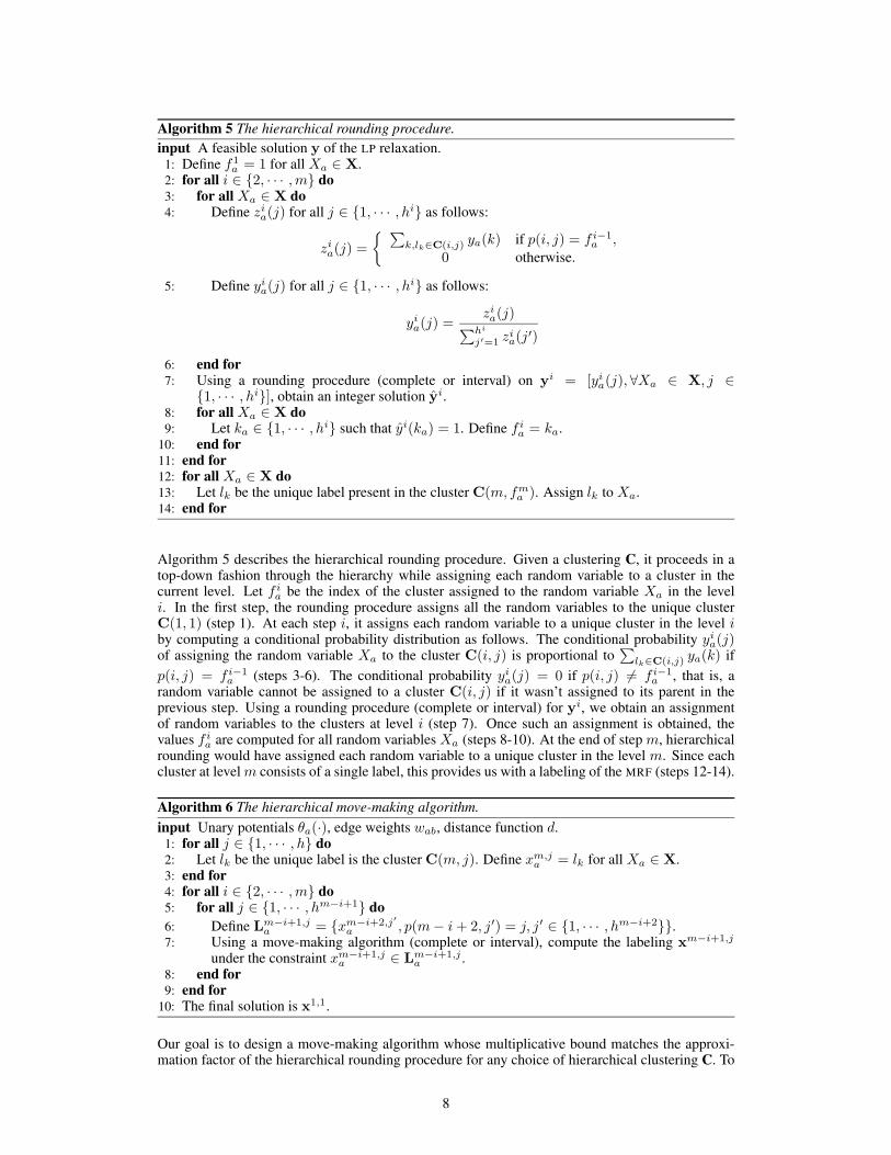
Algorithm 5 describes the hierarchical rounding procedure. Given a clustering C, it proceeds in atop-down fashion through the hierarchy while assigning each random variable to a cluster in thecurrent level. Let f i
a be the index of the cluster assigned to the random variable Xa in the leveli. In the first step, the rounding procedure assigns all the random variables to the unique clusterC(1, 1) (step 1). At each step i, it assigns each random variable to a unique cluster in the level iby computing a conditional probability distribution as follows. The conditional probability yia(j)of assigning the random variable Xa to the cluster C(i, j) is proportional to
∑
lk∈C(i,j) ya(k) if
p(i, j) = f i−1a (steps 3-6). The conditional probability yia(j) = 0 if p(i, j) 6= f i−1
a , that is, arandom variable cannot be assigned to a cluster C(i, j) if it wasn’t assigned to its parent in theprevious step. Using a rounding procedure (complete or interval) for yi, we obtain an assignmentof random variables to the clusters at level i (step 7). Once such an assignment is obtained, thevalues f i
a are computed for all random variables Xa (steps 8-10). At the end of step m, hierarchicalrounding would have assigned each random variable to a unique cluster in the level m. Since eachcluster at level m consists of a single label, this provides us with a labeling of the MRF (steps 12-14).
Algorithm 6 The hierarchical move-making algorithm.
input Unary potentials θa(·), edge weights wab, distance function d.1: for all j ∈ {1, · · · , h} do2: Let lk be the unique label is the cluster C(m, j). Define xm,j
a = lk for all Xa ∈ X.3: end for4: for all i ∈ {2, · · · ,m} do5: for all j ∈ {1, · · · , hm−i+1} do
6: Define Lm−i+1,ja = {xm−i+2,j′
a , p(m− i+ 2, j′) = j, j′ ∈ {1, · · · , hm−i+2}}.7: Using a move-making algorithm (complete or interval), compute the labeling xm−i+1,j
under the constraint xm−i+1,ja ∈ Lm−i+1,j
a .8: end for9: end for
10: The final solution is x1,1.
Our goal is to design a move-making algorithm whose multiplicative bound matches the approxi-mation factor of the hierarchical rounding procedure for any choice of hierarchical clustering C. To
8

this end, we propose the hierarchical move-making algorithm, which extends the hierarchical graphcuts approach for hierarchically well-separated tree (HST) metrics proposed in [15]. Algorithm 6provides its main steps. In contrast to hierarchical rounding, the move-making algorithm traversesthe hierarchy in a bottom-up fashion while computing a labeling for each cluster in the current level.Let xi,j be the labeling corresponding to the cluster C(i, j). At the first step, when considering thelevel m of the clustering, all the random variables are assigned the same label. Specifically, xm,j
a
is equal to the unique label contained in the cluster C(m, j) (steps 1-3). At step i, it computes thelabeling xm−i+1,j for each cluster C(m− i+1, j) by using the labelings computed in the previousstep. Specifically, it restricts the label assigned to a random variable Xa in the labeling xm−i+1,j
to the subset of labels that were assigned to it by the labelings corresponding to the children ofC(m − i + 1, j) (step 6). Under this restriction, the labeling xm−i+1,j is computed by approxi-mately minimizing the energy using a move-making algorithm (step 7). Implicit in our descriptionis the assumption that that we will use a move-making algorithm (complete or interval) in step 7 ofAlgorithm 6 whose multiplicative bound matches the approximation factor of the rounding proce-dure (complete or interval) used in step 7 of Algorithm 5. Note that, unlike the hierarchical graphcuts approach [15], the hierarchical move-making algorithm can be used for any arbitrary clusteringand not just the one specified by an HST metric.
The following theorem establishes the theoretical guarantees of the hierarchical move-making algo-rithm and the hierarchical rounding procedure.
Theorem 3. The tight multiplicative bound of the hierarchical move-making algorithm is equal tothe tight approximation factor of the hierarchical rounding procedure.
The proof of the above theorem is given in Appendix C. The following known result is its corollary.
Corollary 6. The multiplicative bound of the hierarchical move-making algorithm is O(1) for anHST metric distance.
The above corollary follows from the approximation factor of the hierarchical rounding procedureproved in [11], but it was independently proved in [15]. It is worth noting that the above resultwas also used to obtain an approximation factor of O(log h) for the general metric labeling problemin [11] and a matching multiplicative bound of O(log h) in [15].
Note that hierarchical move-making solves a series of problems defined on a smaller label set. Sincethe complexity of complete and interval move-making is superlinear in the number of labels, it canbe verified that the hierarchical move-making algorithm is at most as computationally complex asthe complete move-making algorithm (corresponding to the case when the clustering consists ofonly one cluster that contains all the labels). Hence, hierarchical move-making is significantly fasterthan solving the LP relaxation.
6 Experiments
We demonstrate the efficacy of rounding-based moves by comparing them to several state of the artmethods using both synthetic and real data.
6.1 Synthetic Experiments
Data. We generated random grid MRFs of size 100×100, where each random variable can take oneof 10 labels. The unary potentials were sampled from a uniform distribution over [0, 10]. The edgeweights were sampled from a uniform distribution over [0, 3]. We considered four types of pairwisepotentials: (i) truncated linear metric, where the truncation is sampled from a uniform distributionover [1, 5]; (ii) truncated quadratic metric, where the truncation is sampled from a uniform distribu-tion over [1, 25]; (iii) random metrics, generated by computing the shortest path on graphs whosevertices correspond to the labels and whose edge lengths are uniformly distributed over [1, 10]; (iv)random semi-metrics, where the distance between two labels is sampled from a uniform distributionover [1, 10]. For each type of pairwise potentials, we generated 500 different MRFs.
Methods. We report results obtained by the following state of the art methods: (i) belief propa-gation (BP) [18]; (ii) sequential tree-reweighted message passing (TRW) [12], which optimizes thedual of the LP relaxation, and provides comparable results to other LP relaxation based approaches;(iii) expansion algorithm (EXP) [4]; and (iv) swap algorithm (SWAP) [3]. We compare the above
9

0 2 4 6 8 10 124.8
5
5.2
5.4
5.6
5.8
6
6.2
6.4x 10
4
Time (sec)
Energ
y
BPTRWDUALEXPSWAPINTHIER
0 5 10 154
5
6
7
8
9x 10
4
Time (sec)
En
erg
y
BPTRWDUALEXPSWAPINTHIER
Truncated Linear Truncated Quadratic
0 2 4 6 8 105.1
5.15
5.2
5.25
5.3
5.35
5.4
5.45x 10
4
Time (sec)
En
erg
y
BPTRWDUALEXPSWAPHIER
0 2 4 6 8 105.1
5.15
5.2
5.25
5.3
5.35
5.4
5.45
5.5x 10
4
Time (sec)
En
erg
y
BPTRWDUALEXPSWAPHIER
Metric Semi-Metric
Figure 1: Results for the synthetic dataset. The x-axis shows the time in seconds, while the y-axisshows the energy value. The dashed line shows the value of the dual of the LP obtained by TRW.Best viewed in color.
methods to a hierarchy move-making algorithm (HIER), where a set of hierarchies is obtained by ap-proximating a given (semi-)metric as a mixture of r-HST metrics using the method defined in [6]. Werefer the reader to [6, 15] for details. Each subproblem of the hierarchical move-making algorithmis solved by interval move-making with interval length q = 1 (which corresponds to the expansionalgorithm). In addition, for the truncated linear and truncated quadratic cases, we present results ofinterval move-making (INT) using the optimal interval length reported in [16].
Results. Fig. 1 shows the results of the above methods. In terms of the energy, TRW is the mostaccurate. However, it is slow as it optimizes the dual of the LP relaxation. The labelings obtainedby BP have high energy values. The standard move-making algorithms, EXP and SWAP, are fast dueto the use of efficient minimum st-cut solvers. However, they are not as accurate as TRW. For thetruncated linear and quadratic pairwise potentials, INT provides labelings with comparable energy tothose of TRW, and is also computationally efficient. However, for general metrics and semi-metrics,it is not obvious how to obtain the optimal interval length. The HIER method is more generallyapplicable as there exist standard methods to approximate a (semi-)metric with a mixture of r-HST
metrics [6]. It provides very accurate labelings (comparable to TRW), and is efficient in practice asit relies on solving each subproblem using an iterative move-making algorithm.
6.2 Dense Stereo Correspondence
Data. Given two epipolar rectified images of the same scene, the problem of dense stereo corre-spondence requires us to obtain a correspondence between the pixels of the images. This problem
10

can be modeled as metric labeling, where the random variables represent the pixels of one of theimages, and the labels represent the disparity values. A disparity label li for a random variableXa representing a pixel (ua, va) of an image indicates that its corresponding pixel lies in location(ua + i, va). For the above problem, we use the unary potentials and edge weights that are specifiedin [21]. We use two types of pairwise potentials: (i) truncated linear with the truncation set at 4; and(ii) truncated quadratic with the truncation set at 16.
Methods. We report results on all the baseline methods that were used in the synthetic experi-ments, namely, BP, TRW, EXP, and SWAP. Since the pairwise potentials are either truncated linearor truncated quadratic, we report results for the interval move-making algorithm INT, which usesthe optimal value of the interval length. We also show the results obtained by the hierarchicalmove-making algorithm (HIER), where once again the hierarchies are obtained by approximatingthe (semi-)metric as a mixture of r-HST metrics.
Results. Fig. 2-Fig. 7 shows the results for various standard pairs of images. Note that, similarto the synthetic experiments, TRW is the most accurate in terms of energy, but it is computationallyinefficient. The results obtained by BP are not accurate. The standard move-making algorithms, EXP
and SWAP, are fast but not as accurate as TRW. Among the rounding-based move-making algorithmsINT is slower as it solves a minimum st-cut problem on a large graph at each iteration. In contrast,HIER uses an interval length of 1 for each subproblem and is therefore more efficient. The energyobtained by HIER is comparable to TRW.
Image 1 Image 2 Ground Truth
BP TRW SWAPTime=9.1s, Energy=686350 Time=55.8s, Energy=654128 Time=4.4s, Energy=668031
EXP INT HIERTime=3.3s, Energy=657005 Time=87.2s, Energy=656945 Time=34.6s, Energy=654557
Figure 2: Results for the ‘tsukuba’ image pair with truncated linear pairwise potentials.
11

Image 1 Image 2 Ground Truth
BP TRW SWAPTime=29.9s, Energy=1586856 Time=115.9s, Energy=1415343 Time=7.1s, Energy=1562459
EXP INT HIERTime=5.1s, Energy=1546777 Time=275.6s, Energy=1533114 Time=40.7s, Energy=1499134
Figure 3: Results for the ‘tsukuba’ image pair with truncated quadratic pairwise potentials.
7 Discussion
For any general distance function that can be used to specify the (semi-)metric labeling problem, weproved that the approximation factor of a large family of parallel rounding procedures is matchedby the multiplicative bound of move-making algorithms. This generalizes previously known resultson the guarantees of move-making algorithms in two ways: (i) in contrast to previous results [15,16, 23] that focused on special cases of distance functions, our results are applicable to arbitrarysemi-metric distance functions; and (ii) the guarantees provided by our theorems are tight. Ourexperiments confirm that the rounding-based move-making algorithms provide similar accuracy tothe LP relaxation, while being significantly faster due to the use of efficient minimum st-cut solvers.
Several natural questions arise. What is the exact characterization of the rounding procedures forwhich it is possible to design matching move-making algorithms? Can we design rounding-basedmove-making algorithms for other combinatorial optimization problems? Answering these ques-tions will not only expand our theoretical understanding, but also result in the development of effi-cient and accurate algorithms.
Acknowledgements. This work is funded by the European Research Council under the Euro-pean Community’s Seventh Framework Programme (FP7/2007-2013)/ERC Grant agreement num-ber 259112.
12

Image 1 Image 2 Ground Truth
BP TRW SWAPTime=16.4s, Energy=3003629 Time=105.2s, Energy=2943481 Time=7.7s, Energy=2954819
EXP INT HIERTime=11.5s, Energy=2953157 Time=273.1s, Energy=2959133 Time=105.7s, Energy=2946177
Figure 4: Results for the ‘venus’ image pair with truncated linear pairwise potentials.
References
[1] A. Archer, J. Fakcharoenphol, C. Harrelson, R. Krauthgamer, K. Talvar, and E. Tardos. Ap-proximate classification via earthmover metrics. In SODA, 2004.
[2] Y. Boykov and V. Kolmogorov. An experimental comparison of min-cut/max-flow algorithmsfor energy minimization in vision. PAMI, 2004.
[3] Y. Boykov, O. Veksler, and R. Zabih. Markov random fields with efficient approximations. InCVPR, 1998.
[4] Y. Boykov, O. Veksler, and R. Zabih. Fast approximate energy minimization via graph cuts. InICCV, 1999.
[5] C. Chekuri, S. Khanna, J. Naor, and L. Zosin. Approximation algorithms for the metric labelingproblem via a new linear programming formulation. In SODA, 2001.
[6] J. Fakcharoenphol, S. Rao, and K. Talwar. A tight bound on approximating arbitrary metricsby tree metrics. In STOC, 2003.
13

Image 1 Image 2 Ground Truth
BP TRW SWAPTime=54.3s, Energy=4183829 Time=223.0s, Energy=3080619 Time=22.8s, Energy=3240891
EXP INT HIERTime=30.3s, Energy=3326685 Time=522.3s, Energy=3216829 Time=113s, Energy=3210882
Figure 5: Results for the ‘venus’ image pair with truncated quadratic pairwise potentials.
[7] B. Flach and D. Schlesinger. Transforming an arbitrary minsum problem into a binary one.Technical report, TU Dresden, 2006.
[8] A. Globerson and T. Jaakkola. Fixing max-product: Convergent message passing algorithmsfor MAP LP-relaxations. In NIPS, 2007.
[9] A. Gupta and E. Tardos. A constant factor approximation algorithm for a class of classificationproblems. In STOC, 2000.
[10] T. Hazan and A. Shashua. Convergent message-passing algorithms for inference over generalgraphs with convex free energy. In UAI, 2008.
[11] J. Kleinberg and E. Tardos. Approximation algorithms for classification problems with pair-wise relationships: Metric labeling and Markov random fields. In STOC, 1999.
[12] V. Kolmogorov. Convergent tree-reweighted message passing for energy minimization. PAMI,2006.
[13] N. Komodakis, N. Paragios, and G. Tziritas. MRF optimization via dual decomposition:Message-passing revisited. In ICCV, 2007.
14

Image 1 Image 2 Ground Truth
BP TRW SWAPTime=47.5s, Energy=1771965 Time=317.7s, Energy=1605057 Time=35.2s, Energy=1606891
EXP INT HIERTime=26.5s, Energy=1603057 Time=878.5s, Energy=1606558 Time=313.7s, Energy=1596279
Figure 6: Results for the ‘teddy’ image pair with truncated linear pairwise potentials.
[14] A. Koster, C. van Hoesel, and A. Kolen. The partial constraint satisfaction problem: Facetsand lifting theorems. Operations Research Letters, 1998.
[15] M. P. Kumar and D. Koller. MAP estimation of semi-metric MRFs via hierarchical graph cuts.In UAI, 2009.
[16] M. P. Kumar and P. Torr. Improved moves for truncated convex models. In NIPS, 2008.
[17] R. Manokaran, J. Naor, P. Raghavendra, and R. Schwartz. SDP gaps and UGC hardness formultiway cut, 0-extension and metric labeling. In STOC, 2008.
[18] J. Pearl. Probabilistic Reasoning in Intelligent Systems: Networks of Plausible Inference.Morgan Kauffman, 1998.
[19] P. Ravikumar, A. Agarwal, and M. Wainwright. Message-passing for graph-structured linearprograms: Proximal projections, convergence and rounding schemes. In ICML, 2008.
[20] M. Schlesinger. Syntactic analysis of two-dimensional visual signals in noisy conditions.Kibernetika, 1976.
[21] R. Szeliski, R. Zabih, D. Scharstein, O. Veksler, V. Kolmogorov, A. Agarwala, M. Tappen, andC. Rother. A comparative study of energy minimization methods for Markov random fieldswith smoothness-based priors. PAMI, 2008.
15
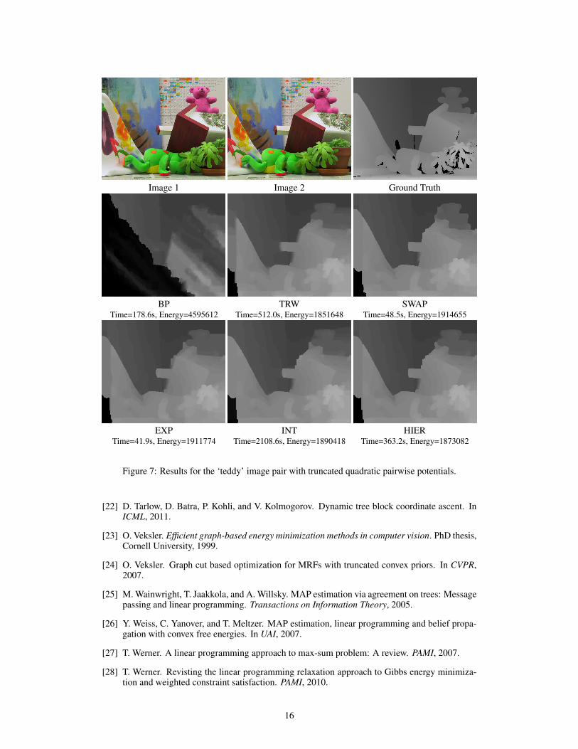
Image 1 Image 2 Ground Truth
BP TRW SWAPTime=178.6s, Energy=4595612 Time=512.0s, Energy=1851648 Time=48.5s, Energy=1914655
EXP INT HIERTime=41.9s, Energy=1911774 Time=2108.6s, Energy=1890418 Time=363.2s, Energy=1873082
Figure 7: Results for the ‘teddy’ image pair with truncated quadratic pairwise potentials.
[22] D. Tarlow, D. Batra, P. Kohli, and V. Kolmogorov. Dynamic tree block coordinate ascent. InICML, 2011.
[23] O. Veksler. Efficient graph-based energy minimization methods in computer vision. PhD thesis,Cornell University, 1999.
[24] O. Veksler. Graph cut based optimization for MRFs with truncated convex priors. In CVPR,2007.
[25] M. Wainwright, T. Jaakkola, and A. Willsky. MAP estimation via agreement on trees: Messagepassing and linear programming. Transactions on Information Theory, 2005.
[26] Y. Weiss, C. Yanover, and T. Meltzer. MAP estimation, linear programming and belief propa-gation with convex free energies. In UAI, 2007.
[27] T. Werner. A linear programming approach to max-sum problem: A review. PAMI, 2007.
[28] T. Werner. Revisting the linear programming relaxation approach to Gibbs energy minimiza-tion and weighted constraint satisfaction. PAMI, 2010.
16
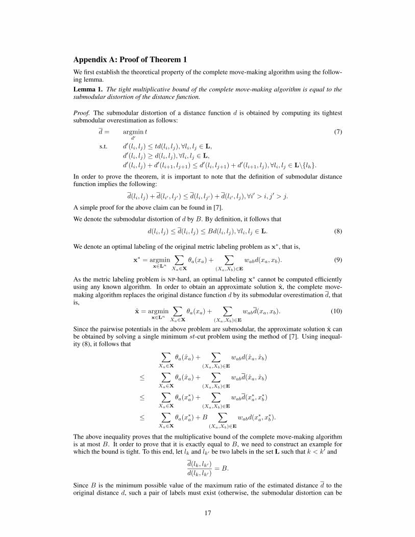
Appendix A: Proof of Theorem 1
We first establish the theoretical property of the complete move-making algorithm using the follow-ing lemma.
Lemma 1. The tight multiplicative bound of the complete move-making algorithm is equal to thesubmodular distortion of the distance function.
Proof. The submodular distortion of a distance function d is obtained by computing its tightestsubmodular overestimation as follows:
d = argmind′
t (7)
s.t. d′(li, lj) ≤ td(li, lj), ∀li, lj ∈ L,
d′(li, lj) ≥ d(li, lj), ∀li, lj ∈ L,
d′(li, lj) + d′(li+1, lj+1) ≤ d′(li, lj+1) + d′(li+1, lj), ∀li, lj ∈ L\{lh}.In order to prove the theorem, it is important to note that the definition of submodular distancefunction implies the following:
d(li, lj) + d(li′ , lj′) ≤ d(li, lj′) + d(li′ , lj), ∀i′ > i, j′ > j.
A simple proof for the above claim can be found in [7].
We denote the submodular distortion of d by B. By definition, it follows that
d(li, lj) ≤ d(li, lj) ≤ Bd(li, lj), ∀li, lj ∈ L. (8)
We denote an optimal labeling of the original metric labeling problem as x∗, that is,
x∗ = argminx∈Ln
∑
Xa∈X
θa(xa) +∑
(Xa,Xb)∈E
wabd(xa, xb). (9)
As the metric labeling problem is NP-hard, an optimal labeling x∗ cannot be computed efficientlyusing any known algorithm. In order to obtain an approximate solution x, the complete move-
making algorithm replaces the original distance function d by its submodular overestimation d, thatis,
x = argminx∈Ln
∑
Xa∈X
θa(xa) +∑
(Xa,Xb)∈E
wabd(xa, xb). (10)
Since the pairwise potentials in the above problem are submodular, the approximate solution x canbe obtained by solving a single minimum st-cut problem using the method of [7]. Using inequal-ity (8), it follows that
∑
Xa∈X
θa(xa) +∑
(Xa,Xb)∈E
wabd(xa, xb)
≤∑
Xa∈X
θa(xa) +∑
(Xa,Xb)∈E
wabd(xa, xb)
≤∑
Xa∈X
θa(x∗a) +
∑
(Xa,Xb)∈E
wabd(x∗a, x
∗b)
≤∑
Xa∈X
θa(x∗a) +B
∑
(Xa,Xb)∈E
wabd(x∗a, x
∗b).
The above inequality proves that the multiplicative bound of the complete move-making algorithmis at most B. It order to prove that it is exactly equal to B, we need to construct an example forwhich the bound is tight. To this end, let lk and lk′ be two labels in the set L such that k < k′ and
d(lk, lk′)
d(lk, lk′)= B.
Since B is the minimum possible value of the maximum ratio of the estimated distance d to theoriginal distance d, such a pair of labels must exist (otherwise, the submodular distortion can be
17
reduced further). Let us assume that there exists an lj ∈ L such that j < k. Other cases (where
j > k′ or k < j < k′) can be handled similarly. Note that since d is submodular, it follows that
d(lk, lj) + d(lj , lk′) ≥ d(lk, lk′). (11)
We define a metric labeling problem over two random variables Xa and Xb connected by an edgewith weight wab = 1. The unary potentials are defined as follows:
θa(i) =
0, if i = k,d(lk,lk′ )+d(lk,lj)−d(lj ,lk′ )
2 , if i = j,∞ otherwise,
θb(i) =
0, if i = k′,d(lk,lk′ )−d(lk,lj)+d(lj ,lk′ )
2 , if i = j,∞ otherwise.
For the above metric labeling problem, it can be verified that an optimal solution x∗ of problem (9)is the following: x∗
a = lk and x∗b = lk′ . Furthermore, using inequality (11), it can be shown that
the following is an optimal solution of problem (10): xa = lj and xb = lj . In other words, x is avalid approximate labeling provided by the complete move-making algorithm. The labelings x∗ andx satisfy the following equality:
∑
Xa∈X
θa(xa) +∑
(Xa,Xb)∈E
wabd(xa, xb) =∑
Xa∈X
θa(x∗a) +B
∑
(Xa,Xb)∈E
wabd(x∗a, x
∗b).
Therefore, the tight multiplicative bound of the complete move-making algorithm is exactly equalto the submodular distortion of the distance function d.
We now turn our attention to the complete rounding procedure for the LP relaxation. Before wecan establish its tight approximation factor, we need to compute the expected distance between thelabels assigned to a pair of neighboring random variables. Recall that, in our notation, we denote afeasible solution of the LP relaxation by y. For any feasible solution y, we define ya as the vectorwhose elements are the unary variables of y for the random variable Xa ∈ X, that is,
ya = [ya(i), ∀li ∈ L]. (12)
Similarly, we define yab as the vector whose elements are the pairwise variables of y for the neigh-boring random variables (Xa, Xb) ∈ E, that is,
yab = [yab(i, j), ∀li, lj ∈ L]. (13)
Furthermore, using ya, we define Ya as
Ya(i) =
i∑
j=1
ya(j).
In other words, if ya is interpreted as the probability distribution over the labels of Xa, then Ya isthe corresponding cumulative distribution.
Given a feasible solution y, we denote the integer solution obtained using the complete roundingprocedure as y. The distance between the two labels encoded by vectors ya and yb will be denoted
by d(ya, yb). In other words, if fa and fb are the indices of the labels assigned to Xa and Xb (that
is, ya(fa) = 1 and yb(fb) = 1), then d(ya, yb) = d(lfa, l
fb).
The following shorthand notation would be useful for our analysis.
D1(i) =1
2(d(li, l1) + d(li, lh)− d(li+1, l1)− d(li+1, lh)) , ∀i ∈ {1, · · · , h− 1}, (14)
D2(i, j) =1
2(d(li, lj+1) + d(li+1, lj)− d(li, lj)− d(li+1, lj+1)) , ∀i, j ∈ {1, · · · , h− 1}.
Using the above notation, we can state the following lemma on the expected distance of the roundedsolution for two neighboring random variables.
18

Lemma 2. Let y be a feasible solution of the LP relaxation, Ya and Yb be cumulative distributionsof ya and yb, and y be the integer solution obtained by the complete rounding procedure for y.Then, the following equation holds true:
E(d(ya, yb)) =h−1∑
i=1
Ya(i)D1(i) +h−1∑
j=1
Yb(j)D1(j) +h−1∑
i=1
h−1∑
j=1
|Ya(i)− Yb(j)|D2(i, j).
Proof. We define fa and fb to be the indices of the labels assigned to Xa and Xb by the rounded
integer solution y. In other words, ya(i) = 1 if and only if i = fa and yb(j) = 1 if and only if
j = fb. We define binary variables za(i) and zb(j) as follows:
za(i) =
{
1 if i ≤ fa,0 otherwise,
zb(j) =
{
1 if j ≤ fb,0 otherwise.
For complete rounding, it can be verified that
E(za(i)) = Ya(i). (15)
Furthermore, we also define binary variables zab(i, j) that indicate whether i and j are contained
within the interval defined by fa and fb. Formally,
zab(i, j) =
{
1 if min{i, j} ≥ min{fa, fb} and max{i, j} < max{fa, fb},0 otherwise.
For complete rounding, it can be verified that
E(zab(i, j)) = |Ya(i)− Yb(j)|. (16)
Using the result of [7], we know that
d(ya, yb) =h−1∑
i=1
za(i)D1(i) +h−1∑
j=1
zb(j)D1(j) +h−1∑
i=1
h−1∑
j=1
zab(i, j)D2(i, j).
The proof of the lemma follows by taking the expectation of the LHS and the RHS of the aboveequation and simplifying the RHS using the linearity of expectation and equations (15) and (16).
In order to state the next lemma, we require the definition of uncrossing pairwise variables. Givenunary variables ya and yb, the pairwise variable vector y′
ab is called uncrossing with respect to ya
and yb if it satisfies the following properties:
h∑
j=1
y′ab(i, j) = ya(i), ∀i ∈ {1, 2, · · · , h},
h∑
i=1
y′ab(i, j) = yb(i), ∀j ∈ {1, 2, · · · , h},
y′ab(i, j) ≥ 0, ∀i, j ∈ {1, 2, · · · , h},min{y′ab(i, j′), y′ab(i′, j)} = 0, ∀i, j, i′, j′ ∈ {1, 2, · · · , h}, i < i′, j < j′. (17)
The following lemma establishes a connection between the expected distance between the labelsassigned by complete rounding and the pairwise cost specified by uncrossing pairwise variables.
Lemma 3. Let y be a feasible solution of the LP relaxation, and y be the integer solution obtainedby the complete rounding procedure for y. Furthermore, let y′
ab be uncrossing pairwise variableswith respect to ya and yb. Then, the following equation holds true:
E(d(ya, yb)) =
h∑
i=1
h∑
j=1
d(li, lj)y′ab(i, j).
19

Proof. We define Ya and Yb to be the cumulative distributions corresponding to ya and yb respec-tively. We claim that the uncrossing property (17) implies the following condition:
i′∑
i=1
j′∑
j=1
y′ab(i, j) = min{Ya(i′), Yb(j
′)}, ∀i′, j′ ∈ {1, · · · , h}. (18)
To prove this claim, assume that Ya(i′) < Yb(j
′). The other cases can be handled similarly. Sincey′ab satisfies the constraints of the LP relaxation, it follows that:
h∑
i=1
j′∑
j=1
y′ab(i, j) = Yb(j′),
i′∑
i=1
h∑
j=1
y′ab(i, j) = Ya(i′). (19)
Since the LHS of equality (18) is less than or equal to the LHS of both the above equations, it followsthat
i′∑
i=1
j′∑
j=1
y′ab(i, j) ≤ min{Ya(i′), Yb(j
′)}. (20)
Therefore, there must exist a k > i′ and k′ ≤ j′ such that y′ab(k, k′) 6= 0. Otherwise, the LHS
in the above inequality will be exactly equal to Yb(j′), which would result in a contradiction. By
the uncrossing property (17), we know that min{y′ab(i, j), y′ab(k, k′)} = 0 if i ≤ i′ and j > j′.Therefore, y′ab(i, j) = 0 for all i ≤ i′ and j > j′, which proves the claim.
Combining equations (19) and (20), we get the following:
i′∑
i=1
h∑
j=j′+1
y′ab(i, j) +
h∑
i=i′+1
j′∑
j=1
y′ab(i, j) = |Ya(i)− Yb(j)|, ∀i′, j′ ∈ {1, · · · , h}.
By solving for y′ab using the above equations, we get
h∑
i=1
h∑
j=1
d(li, lj)y′ab(i, j) =
h−1∑
i=1
Ya(i)D1(i) +
h−1∑
j=1
Yb(j)D1(j) +
h−1∑
i=1
h−1∑
j=1
|Ya(i)− Yb(j)|D2(i, j).
Using the previous lemma, this proves that
E(d(ya, yb)) =h∑
i=1
h∑
j=1
d(li, lj)y′ab(i, j).
Our next lemma establishes that uncrossing pairwise variables are optimal for submodular distancefunctions.
Lemma 4. Let y′ab be the uncrossing pairwise variables with respect to the unary variables ya and
yb. Let d : L × L → R+ be a submodular distance function. Then the following condition holds
true:
y′ab = argmin
yab
h∑
i=1
h∑
j=1
d(i, j)yab(i, j), (21)
s.t.
h∑
j=1
yab(i, j) = ya(i), ∀i ∈ {1, · · · , h},
h∑
i=1
yab(i, j) = yb(j), ∀j ∈ {1, · · · , h},
yab(i, j) ≥ 0, ∀i, j ∈ {1, · · · , h}.
20

Proof. We prove the lemma by contradiction. Suppose that the optimal solution to the above prob-lem is y′′
ab, which is not uncrossing. Let
min{y′′ab(i, j′), y′′ab(i′, j)} = λ 6= 0,
where i < i′ and j < j′. Since d is submodular, it implies that
d(li, lj) + d(li′ , lj′) ≤ d(li, lj′) + d(li′ , lj).
Therefore the objective function of problem (21) can be reduced further by the following modifica-tion:
y′′ab(i, j′)← y′′ab(i, j
′)− λ, y′′ab(i′, j)← y′′ab(i
′, j)− λ,
y′′ab(i, j)← y′′ab(i, j) + λ, y′′ab(i′, j′)← y′′ab(i
′, j′) + λ.
The resulting contradiction proves our claim that the uncrossing pairwise variables y′ab are an opti-
mal solution of problem (21).
Using the above lemmas, we will now obtain the tight approximation factor of the complete roundingprocedure.
Lemma 5. The tight approximation factor of the complete rounding procedure is equal to the sub-modular distortion of the distance function.
Proof. We denote a feasible fractional solution of the LP relaxation by y and the rounded solution byy. Consider a pair of neighboring random variables (Xa, Xb) ∈ X. We define uncrossing pairwisevariables y′
ab with respect to ya and yb. Using lemmas 3 and 4, the approximation factor of thecomplete rounding procedure can be shown to be at most B as follows:
E(d(ya, yb)) =
h∑
i=1
h∑
j=1
d(li, lj)y′ab(i, j)
≤h∑
i=1
h∑
j=1
d(li, lj)y′ab(i, j)
≤h∑
i=1
h∑
j=1
d(li, lj)yab(i, j)
≤ B
h∑
i=1
h∑
j=1
d(li, lj)yab(i, j).
In order to prove that the approximation factor of the complete rounding is exactly B, we need anexample where the above inequality holds as an equality. The key to obtaining a tight example liesin the Lagrangian dual of problem (7). In order to specify its dual, we need three types of dualvariables. The first type, denoted by α(i, j), corresponds to the constraint
d′(li, lj) ≤ td(li, lj).
The second type, denoted by β(i, j), corresponds to the constraint
d′(li, lj) ≥ d(li, lj).
The third type, denoted by γ(i, j), corresponds to the constraint
d′(li, lj) + d′(li+1, lj+1) ≤ d′(li, lj+1) + d′(li+1, lj).
Using the above variables, the dual of problem (7) is given by
max
h∑
i=1
h∑
j=1
d(li, lj)β(i, j) (22)
s.t.
h∑
i=1
h∑
j=1
d(li, lj)α(i, j) = 1,
β(i, j) = α(i, j)− γ(i, j − 1)− γ(i− 1, j) + γ(i− 1, j − 1) + γ(i, j),
∀i, j ∈ {1, · · · , h},α(i, j) ≥ 0, β(i, j) ≥ 0, γ(i, j) ≥ 0, ∀i, j ∈ {1, · · · , h}.
21

We claim that the above dual problem has an optimal solution (α∗,β∗,γ∗) that satisfies the follow-ing property:
min{β∗(i, j′), β∗(i′, j)} = 0, ∀i, i′, j, j′ ∈ {1, · · · , h}, i < i′, j < j′. (23)
We refer to the optimal dual solution β∗ that satisfies the above property as uncrossing dual variablesas it is analogous to uncrossing pairwise variables. The above claim, namely, the existence of anuncrossing optimal dual solution, can be proved by contradiction as follows. Suppose there existsno optimal solution that satisfies the above property. Then consider the following problem, which isthe dual of the problem of finding the tightest submodular overestimate of the submodular function
d:
max
h∑
i=1
h∑
j=1
d(li, lj)β(i, j) (24)
s.t.
h∑
i=1
h∑
j=1
d(li, lj)α(i, j) = 1,
β(i, j) = α(i, j)− γ(i, j − 1)− γ(i− 1, j) + γ(i− 1, j − 1) + γ(i, j),
∀i, j ∈ {1, · · · , h},α(i, j) ≥ 0, β(i, j) ≥ 0, γ(i, j) ≥ 0, ∀i, j ∈ {1, · · · , h}.
By strong duality, problem (24) has an optimal value of 1. However, the optimal solution of prob-lem (22), which is also a feasible solution for problem (24), provides a value strictly greater than 1.This results in a contradiction that proves our claim.
The optimal dual variables that satisfy property (23) allow us to construct an example that provesthat the approximation factor B of the complete rounding procedure is tight. Specifically, we define
yab(i, j) =α∗(i, j)
∑h
i′=1
∑h
j′=1 α∗(i′, j′)
, ∀i, j ∈ {1, · · · , h},
ya(i) =
h∑
j=1
yab(i, j), ∀i ∈ {1, · · · , h},
yb(j) =
h∑
i=1
yab(i, j), ∀j ∈ {1, · · · , h}.
Note that the pairwise variables yab must minimize the pairwise potential corresponding to the unaryvariables ya and yb, that is,
yab = argminyab
∑
li,lj∈L
d(li, lj)yab(i, j) (25)
s.t.∑
lj∈L
yab(i, j) = ya(i), ∀li ∈ L
∑
li∈L
yab(i, j) = yb(j), ∀lj ∈ L
yab(i, j) ≥ 0, ∀li, lj ∈ L.
If the above statement was not true, then the value of the dual problem (22) could be increasedfurther.
We also define the following pairwise variables:
y′ab(i, j) =β∗(i, j)
∑h
i′=1
∑h
j′=1 β∗(i′, j′)
, ∀i, j ∈ {1, · · · , h},
y′a(i) =h∑
j=1
y′ab(i, j), ∀i ∈ {1, · · · , h},
y′b(j) =
h∑
i=1
y′ab(i, j), ∀j ∈ {1, · · · , h}.
22
It can be verified that
y′a(i) = ya(i), y′b(j) = yb(j), ∀i, j ∈ {1, · · · , h}.
The above condition follows from the constraints of problem (22). Due to the uncrossing property ofβ∗, the pairwise variables y′
ab are uncrossing with respect to ya and yb. By lemma 3, this impliesthat
E(d(ya, yb)) =h∑
i=1
h∑
j=1
d(li, lj)y′ab(i, j),
where ya and yb are integer solutions obtained by the complete rounding procedure. By strongduality, it follows that
E(d(ya, yb)) = Bh∑
i=1
h∑
j=1
d(li, lj)yab(i, j). (26)
The existence of an example that satisfies properties (25) and (26) implies that the tight approxima-tion factor of the complete rounding procedure is B.
Lemmas 1 and 5 together prove theorem 1.
Appendix B: Proof of Theorem 2
We begin by establishing the theoretical properties of the interval-move making algorithm. Recallthat, given an interval of labels I = {ls, · · · , le} of at most q consecutive labels and a labeling x, wedefine Ia = I ∪ {xa} for all random variables Xa ∈ X. In order to use the interval move-making
algorithm, we compute a submodular distance function dxa,xb: Ia × Ib → R
+ for all pairs ofneighboring random variables (Xa, Xb) ∈ E as follows:
dxa,xb= argmin
d′
t (27)
s.t. d′(li, lj) ≤ td(li, lj), ∀li ∈ Ia, lj ∈ Ib,
d′(li, lj) ≥ d(li, lj), ∀li ∈ Ia, lj ∈ Ib,
d′(li, lj) + d′(li+1, lj+1) ≤ d′(li, lj+1) + d′(li+1, lj), ∀li, lj ∈ I\{le},d′(li, le) + d′(li+1, xb) ≤ d′(li, xb) + d′(li+1, le), ∀li ∈ I\{le},d′(le, lj) + d′(xa, lj+1) ≤ d′(le, lj+1) + d′(xa, lj), ∀lj ∈ I\{le},d′(le, le) + d(xa, xb) ≤ d′(le, xb) + d′(xa, le).
For any interval I and labeling x, we define the following sets:
V(x, I) = {Xa|Xa ∈ X, xa ∈ I},A(x, I) = {(Xa, Xb)|(Xa, Xb) ∈ E, xa ∈ I, xb ∈ I},B1(x, I) = {(Xa, Xb)|(Xa, Xb) ∈ E, xa ∈ I, xb /∈ I},B2(x, I) = {(Xa, Xb)|(Xa, Xb) ∈ E, xa /∈ I, xb ∈ I},B(x, I) = B1(x) ∪B2(x).
In other words, V(x, I) is the set of all random variables whose label belongs to the interval I.Similarly, A(x, I) is the set of all neighboring random variables such that the labels assigned toboth the random variables belong to the interval I. The set B(x, I) contains the set of all neighboringrandom variables such that only one of the two labels assigned to the two random variables belongsto the interval I. Given the set of all intervals I and a labeling x, we define the following for allxa, xb ∈ L:
D(xa, xb; xa, xb) =∑
I∈I,A(x,I)∋(Xa,Xb)
dxa,xb(xa, xb)
+∑
I∈I,B1(x,I)∋(Xa,Xb)
dxa,xb(xa, xb)
+∑
I∈I,B2(x,I)∋(Xa,Xb)
dxa,xb(xa, xb).
23

Using the above notation, we are ready to state the following lemma on the theoretical guarantee ofthe interval move-making algorithm.
Lemma 6. The tight multiplicative bound of the interval move-making algorithm is equal to
1
qmax
xa,xb,xa,xb∈L,xa 6=xb
D(xa, xb; xa, xb)
d(xa, xb).
Proof. We denote an optimal labeling by x∗ and the estimated labeling by x. Let t ∈ [1, q] bea uniformly distributed random integer. Using t, we define the following set of non-overlappingintervals:
It = {[1, t], [t+ 1, t+ q], · · · , [., h]}.For each interval I ∈ It, we define a labeling xI as follows:
xIa =
{
x∗a if x∗
a ∈ I,xa otherwise.
Since x is the labeling obtained after the interval move-making algorithm converges, it follows that∑
Xa∈X
θa(xa) +∑
(Xa,Xb)∈E
wabdxa,xb(xa, xb) ≤
∑
Xa∈X
θa(xIa) +
∑
(Xa,Xb)∈E
wabdxa,xb(xI
a, xIb).
By canceling out the common terms, we can simplify the above inequality as∑
Xa∈V(x∗,I)
θa(xa)
+∑
(Xa,Xb)∈A(x∗,I)
wabdxa,xb(xa, xb)
+∑
(Xa,Xb)∈B1(x∗,I)
wabdxa,xb(xa, xb)
+∑
(Xa,Xb)∈B2(x∗,I)
wabdxa,xb(xa, xb)
≤∑
Xa∈V(x∗,I)
θa(x∗a)
+∑
(Xa,Xb)∈A(x∗,I)
wabdxa,xb(x∗
a, x∗b)
+∑
(Xa,Xb)∈B1(x∗,I)
wabdxa,xb(x∗
a, xb)
+∑
(Xa,Xb)∈B2(x∗,I)
wabdxa,xb(xa, x
∗b).
We now sum the above inequality over all the intervals I ∈ It. Note that the resulting LHS is atleast equal to the energy of the labeling x when the distance function between the random variables
(Xa, Xb) is dxa,xb. This implies that
∑
Xa∈X
θa(xa) +∑
(Xa,Xb)∈E
wabdxa,xb(xa, xb)
≤∑
Xa∈X
θa(x∗a)
+∑
I∈It
∑
(Xa,Xb)∈A(x∗,I)
wabdxa,xb(x∗
a, x∗b)
+∑
I∈It
∑
(Xa,Xb)∈B1(x∗,I)
wabdxa,xb(x∗
a, xb)
+∑
I∈It
∑
(Xa,Xb)∈B2(x∗,I)
wabdxa,xb(xa, x
∗b).
24
Taking the expectation on both sides of the above inequality with respect to the uniformly distributedrandom integer t ∈ [1, q] proves that the multiplicative bound of the interval move-making algorithmis at most equal to
1
qmax
xa,xb,xa,xb∈L,xa 6=xb
D(xa, xb; xa, xb)
d(xa, xb).
A tight example with two random variables Xa and Xb with wab = 1 can be constructed similar tothe one shown in lemma 1.
We now turn our attention to the interval rounding procedure. Let y be a feasible solution of the LP
relaxation, and y be the integer solution obtained using interval rounding. Once again, we define theunary variable vector ya and the pairwise variable vector yab as specified in equations (12) and (13)respectively. Similar to the previous appendix, we denote the expected distance between ya and yb
as d(ya, yb).
Given an interval I = {ls, · · · , le} of at most q consecutive labels, we define a vector YIa for each
random variable Xa as follows:
Y Ia (i) =
s+i−1∑
j=s
ya(j), ∀i ∈ {1, · · · , e− s+ 1}.
In other words, YIa is the cumulative distribution of ya within the interval I. Furthermore, for each
pair of neighboring random variables (Xa, Xb) ∈ E we define
ZIab = max{Y I
a (e− s+ 1), Y Ib (e− s+ 1)} −min{Y I
a (e− s+ 1), Y Ib (e− s+ 1)},
ZIa(i) = min{Y I
a (i), YIb (e− s+ 1)}, ∀i ∈ {1, · · · , e− s+ 1},
ZIb(j) = min{Y I
b (j), YIa (e− s+ 1)}, ∀j ∈ {1, · · · , e− s+ 1}.
The following shorthand notation would be useful to concisely specify the exact form of d(ya, yb).
DI0 = max
li,lj ,|{li,lj}∩I|=1d(li, lj),
DI1(i) =
1
2(d(ls+i−1, ls) + d(ls+i−1, le)− d(ls+i, ls)− d(ls+i, le)) , ∀i ∈ {1, · · · , e− s},
DI2(i, j) =
1
2(d(ls+i−1, ls+j) + d(ls+i, ls+j−1)− d(ls+i−1, ls+j−1)− d(ls+i, ls+j)) ,
∀i, j ∈ {1, · · · , e− s}.In other words, DI
0 is the maximum distance between two labels such that only one of the two labelslies in the interval I. The terms DI
1 and DI2 are analogous to the terms defined in equation (14).
Using the above notation, we can state the following lemma on the expected distance of the roundedsolution for two neighboring random variables.
Lemma 7. Let y be a feasible solution of the LP relaxation, and y be the integer solution obtainedby the interval rounding procedure for y using the set of intervals I. Then, the following inequalityholds true:
E(d(ya, yb)) ≤1
q
∑
I={ls,··· ,le}∈I
ZIabD
I0 +
e−s∑
i=1
ZIa(i)D
I1(i) +
e−s∑
j=1
ZIb(j)D
I1(j)+
e−s∑
i=1
e−s∑
j=1
|ZIa(i)− ZI
b(j)|DI2(i, j)
.
Proof. We begin the proof by establishing the probability of a random variable Xa being assigneda label in an iteration of the interval rounding procedure. The total number of intervals in the set Iis h + q − 1. Out of all the intervals, each label li is present in q intervals. Thus, the probabilityof choosing an interval that contains the label li is q/(h+ q − 1). Once an interval containing li ischosen, the probability of assigning the label li to Xa is ya(i). Thus, the probability of assigning a
25

label li to Xa is ya(i)q/(h+ q − 1). Summing over all labels li, we observe that the probability ofassigning a label to Xa in an iteration of the interval rounding procedure is q/(h+ q − 1).
Now we consider two neighboring random variables (Xa, Xb) ∈ E. In the current iteration ofinterval rounding, given an interval I, the probability of exactly one of the two random variablesgetting assigned a label in I is exactly equal to ZI
ab. In this case, we have to assume that the expected
distance between the two variables will be the maximum possible, that is, DI0. If both the variables
are assigned a label in I, then a slight modification of lemma 2 gives us the expected distance as
e−s∑
i=1
ZIa(i)D
I1(i) +
e−s∑
j=1
ZIb(j)D
I1(j) +
e−s∑
i=1
e−s∑
j=1
|ZIa(i)− ZI
b(j)|DI2(i, j).
Thus, the expected distance between the labels of Xa and Xb conditioned on at least one of the tworandom variables getting assigned in an iteration is equal to
1
(h+ q − 1)
∑
I={ls,··· ,le}∈I
ZIabD
I0 +
e−s∑
i=1
ZIa(i)D
I1(i) +
e−s∑
j=1
ZIb(j)D
I1(j)+
e−s∑
i=1
e−s∑
j=1
|ZIa(i)− ZI
b(j)|DI2(i, j)
,
where the term 1/(h+q−1) corresponds to the probability of choosing an interval from the set I. In
order to compute d(ya, yb), we need to divide the above term with the probability of at least one ofthe two random variables getting assigned a label in the current iteration. Since the two cumulativedistributions YI
a and YIb can be arbitrarily close to each other without being exactly equal, we can
only lower bound the probability of at least one of Xa and Xb being assigned a label at the currentiteration by the probability of Xa being assigned a label in the current iteration. Since the probabilityof Xa being assigned a label is q/(h+ q − 1), it follows that
E(d(ya, yb)) ≤1
q
∑
I={ls,··· ,le}∈I
ZIabD
I0 +
e−s∑
i=1
ZIa(i)D
I1(i) +
e−s∑
j=1
ZIb(j)D
I1(j)+
e−s∑
i=1
e−s∑
j=1
|ZIa(i)− ZI
b(j)|DI2(i, j)
.
Using the above lemma, we can now establish the theoretical property of the interval roundingprocedure.
Lemma 8. The tight approximation factor of the interval rounding procedure is equal to
1
qmax
xa,xb,xa,xb∈L,xa 6=xb
D(xa, xb; xa, xb)
d(xa, xb).
Proof. Similar to lemma 5, the key to proving the above lemma lies in the dual of problem (27).Given the current labels xa and xb of the random variables Xa and Xb respectively, as well as an
interval I = {ls, · · · , le}, problem (27) computes the tightest submodular overestimation dxa,xb:
Ia × Ib → R+ where Ia = I ∪ {xa} and Ib = I ∪ {xb}. Similar to problem (22), the dual of
problem (27) consists of three types of dual variables. The first type, denoted by α(i, j; xa, xb, I)corresponds to the constraint
d′(li, lj) ≤ td(li, lj).
The second type, denoted by β(i, j; xb, xb, I), corresponds to the constraint
d′(li, lj) ≥ d(li, lj).
26

The third type, denoted by γ(i, j; xa, xb, I), corresponds to the constraint
d′(li, lj) + d′(li+1, lj+1) ≤ d′(li, lj+1) + d′(li+1, lj).
Let (α∗(xa, xb, I),β∗(xa, xb, I),γ
∗(xa, xb, I)) denote an optimal solution of the dual. A modifica-tion of lemma 5 can be used to show that there must exist an optimal solution such that β∗(xa, xb, I)is uncrossing.
We consider the values of xa and xb for which we obtain the tight multiplicative bound of the intervalmove-making algorithm. For these values of xa and xb, we define
yab(i, j; xa, xb) =
∑
I∈I α∗(i, j; xa, xb, I)∑
i′,j′
∑
I∈I α∗(i′, j′; xa, xb, I), ∀i, j ∈ {1, · · · , h},
ya(i; xa, xb) =
h∑
j=1
yab(i, j; xa, xb), ∀i ∈ {1, · · · , h},
yb(j; xa, xb) =h∑
i=1
yab(i, j; xa, xb), ∀j ∈ {1, · · · , h},
y′ab(i, j; xa, xb) =
∑
I∈I β∗(i, j; xa, xb, I)∑
i′,j′
∑
I∈I β∗(i′, j′; xa, xb, I), ∀i, j ∈ {1, · · · , h},
y′a(i; xa, xb) =
h∑
j=1
y′ab(i, j; xa, xb), ∀i ∈ {1, · · · , h},
y′b(j; xa, xb) =h∑
i=1
y′ab(i, j; xa, xb), ∀j ∈ {1, · · · , h}.
The constraints of the dual of problem (27) ensure that
ya(i; xa, xb) = y′a(i; xa, xb), ∀i ∈ {1, · · · , h},yb(j; xa, xb) = y′b(j; xa, xb), ∀j ∈ {1, · · · , h}.
Given the distributions ya(xa, xb) and yb(xa, xb), we claim that the pairwise variables yab(xa, xb)must minimize the pairwise potentials corresponding to these distributions, that is,
yab(xa, xb) = argminyab
∑
li,lj∈L
d(li, lj)yab(i, j)
s.t.∑
lj∈L
yab(i, j) = ya(i; xa, xb), ∀li ∈ L
∑
li∈L
yab(i, j) = yb(j; xa, xb), ∀lj ∈ L
yab(i, j) ≥ 0, ∀li, lj ∈ L.
If the above claim was not true, then we could further increase the value of at least one of the duals ofproblem (27) corresponding to some interval I. Furthermore, since y′
ab(xa, xb) is constructed usingβ∗(xa, xb, I), which is uncrossing, a modification of lemma 3 can be used to show that
d(ya(xa, xb), yb(xa, xb)) =∑
li,lj∈L
d(li, lj)y′ab(i, j; xa, xb).
Here ya(xa, xb) and yb(xa, xb) are the rounded solutions obtained by the interval rounding proce-dure applied to ya(xa, xb) and yb(xa, xb).
By duality, it follows that∑
li,lj∈L d(li, lj)y′ab(i, j; xa, xb)
∑
li,lj∈L d(li, lj)yab(i, j; xa, xb)≤ 1
qmax
xa,xb,xa,xb∈L,xa 6=xb
D(xa, xb; xa, xb)
d(xa, xb).
Strong duality implies that there must exist a set of variables for which the above inequality holdsas an equality. This proves the lemma.
Lemmas 6 and 8 together prove theorem 2.
27

Appendix C: Proof of Theorem 3
Proof. The proof of the above theorem proceeds in a similar fashion to the previous two theorems,namely, by computing the dual of the problems that are used to obtain the tightest submodularoverestimation of the given distance function. In what follows, we provide a brief sketch of theproof and omit the details.
We start with the hierarchical move-making algorithm. Recall that this algorithm computes a label-ing xi,j for each cluster C(i, j) ⊆ L, where C(i, j) denotes the j-th cluster at the i-th level. In orderto obtain a labeling xi,j it makes use of the labelings computed at the (i+ 1)-th level. Specifically,
let Li,ja = {xi+1,j′
a , p(i + 1, j′) = j, j′ ∈ {1, · · · , hi+1}}. In other words, Li,ja is the set of labels
that were assigned to the random variable Xa by the labelings corresponding to the children of thecurrent cluster C(i, j). In order to compute the labeling xi,j , the algorithm has to choose one labelfrom the set Li,j
a . This is achieved either using the complete move-making algorithm or the intervalmove-making algorithm. The algorithm is initialized by define xm,j
a = k for all Xa ∈ X where kis the unique label in the cluster C(m, j) The algorithm terminates by computing x1,1, which is thefinal labeling.
Let the multiplicative bound corresponding to the computation of xi,j be denoted by Bi,j .From the arguments of theorems 1 and 2, it follows that there must exist dual variables(α∗(i, j),β∗(i, j),γ∗(i, j)) that provide an approximation factor that is exactly equal to Bi,j andβ∗(i, j) is uncrossing. For each cluster C(i, j), we define variables δa(k; i, j) for k ∈ Li,j
a asfollows:
δa(k; i, j) =
∑
k′∈Li,j
b
α∗(k, k′; i, j)∑
l∈Li,ja
∑
l′∈Li,j
b
α∗(l, l′; i, j).
Using the above variables we define unary variables ya(k; i, j) for each k ∈ Li,j as follows:
ya(k; 1, 1) = δa(k; 1, 1),
ya(k; i, j) = ya(xi−1,p(i,j)a ; i− 1, p(i, j))δa(k; i, j).
Similarly, we define variables δb(k′; i, j) for each k′ ∈ L
i,jb as follows:
δb(k′; i, j) =
∑
k∈Li,ja
α∗(k, k′; i, j)∑
l∈Li,ja
∑
l′∈Li,j
b
α∗(l, l′; i, j).
Using the above variables, we define unary variables yb(k′; i, j) for each k′ ∈ L
i,jb as follows:
yb(k′; 1, 1) = δb(k
′; 1, 1),
yb(k′; i, j) = ya(x
i−1,p(i,j)a ; i− 1, p(i, j))δb(k
′; i, j).
Since each cluster in the m-th level contains a single unique label, it follows that
ya = [ya(xm,ja ;m, j), ∀j = 1, · · · , h],
yb = [yb(xm,jb ;m, j), ∀j = 1, · · · , h],
are valid unary variables for the LP relaxation. It can be shown that applying the hierarchical round-ing procedure on the variables ya and yb provides an approximation factor that is exactly equal tothe multiplicative bound of the hierarchical move-making algorithm.
28