Department of Mechanical and Aerospace Engineering

Routes to Low-Cost Yield Improvement for

Small-Scale Biogas Digesters

Author: Russell Stuart Pepper

Supervisor: Professor Joseph Clarke

A thesis submitted in partial fulfilment for the requirement of the degree

Master of Science

Sustainable Engineering: Renewable Energy Systems and the Environment

2015

Copyright Declaration

This thesis is the result of the author’s original research. It has been composed by the

author and has not been previously submitted for examination which has led to the

award of a degree.

The copyright of this thesis belongs to the author under the terms of the United

Kingdom Copyright Acts as qualified by University of Strathclyde Regulation 3.50.

Due acknowledgement must always be made of the use of any material contained in,

or derived from, this thesis.

Signed: Date: 02/09/2015

3

Acknowledgements

Thanks to my supervisor, Professor Joseph Clarke, who gave me the advice and

assistance I needed to complete this project. Additionally Dr Paul Strachan has been

an excellent course director for RESE, always very helpful and informative.

Thanks also to Matthew Geraghty, Andrew Roscoe, Maureen Cloonan and Jean

Currie for giving me permission to use their modelling tool in this study.

My parents John and Wendy are always there for me and have always given me the

help and assistance I need to follow my ambitions; my master’s year here in Glasgow

would not have been possible without them.

And finally thanks to my partner, Karolina, who encouraged me to take this course

and moved to Scotland with me so I could take it. She’s supported me and given me a

lot of help and advice in completing this thesis – this last year would not have been

easy without her.

4

Abstract

Biogas digesters (BDs) have the potential to reduce greenhouse gas (GHG) emissions

through burning methane released from manure and landfill, rather than allowing it to

escape into the atmosphere. If used in developing countries, they reduce the demand

for solid fuel which is the main source of cooking and heating energy which

contributes to deforestation as well as releasing GHGs.

Whilst large-scale plants are gaining popularity in more developed countries, they are

less accessible in developing countries due to cost, skill and infrastructure limitations.

The aim of this study was therefore to explore ways in which small-scale plants –

quite common in developing countries – could become more profitable, with minimal

additional investment.

In achieving this, a rudimentary small scale plant was modelled. A systematic

assessment of the addition of components to this plant was then performed using

performance and financial variability factors which were derived from a literature

review. The impacts of these additions were measured, and from the increase in

profit, a “maximum acceptable investment” value was derived for a range of

acceptable payback periods.

It was found that the addition of a second digester increased payback period by 50%.

Additionally, it was found that heating provided the highest yield increase – 22, 44

and 66% for heating at temperatures of 25, 30 and 35ºC respectively. The addition of

a shredder gave a 38% increase and a second digester 11.7%. For combinations of

two or more components, those combinations including heating always provided the

highest yields. It was therefore recommended that the primary focus of future work

be on finding low-cost heating solutions, and secondarily, shredders.

5

Table of Contents

List of Figures ........................................................................................................ 7

List of Tables ......................................................................................................... 8

List of Abbreviations ............................................................................................. 9

List of Symbols .................................................................................................... 10

1. The Role of Biogas Digesters in CO2 Reduction ............................................. 11

2. Possible Improvements to Rudimentary Biogas Digesters ............................. 14

3. Performance Assessment ................................................................................... 18

3.1. Tool Requirements and Selection ................................................................ 18

3.2. Description of Selected Tool ....................................................................... 19

3.3. Tool Adaptation ........................................................................................... 24

3.4. Derivation of Performance Variability Factors ............................................ 27

3.4.1. Single-stage vs. two-stage digestion – biogas yield ................................. 27

3.4.2. Heated digestion – biogas yield ............................................................... 30

3.4.3. Mixers – biogas yield ............................................................................... 33

3.4.4. Shredders – biogas yield .......................................................................... 35

3.5. Derivation of Financial Variability Factors ................................................. 37

3.5.1. Single-stage vs. two-stage digestion – cost .............................................. 37

3.5.2. Heated digestion - cost ............................................................................. 38

3.5.3. Mixers - cost ............................................................................................ 39

3.5.4. Shredders - cost ........................................................................................ 40

3.6. Tool Alteration to Include Variability Factors ............................................. 40

3.7. Tool Validation - Case Study: SBW Lelbach .............................................. 45

3.7.1. Assumptions ............................................................................................. 46

3.7.2. Methane production ................................................................................. 48

3.7.3. Electricity generation ............................................................................... 50

3.7.4. Heat generation ........................................................................................ 50

3.7.5. Financial viability .................................................................................... 51

6

3.7.6. Conclusion on tool accuracy .................................................................... 54

3.8. Tool Modelling for Small-Scale Biogas Digesters ...................................... 55

3.8.1. Case study: household-scale BD in Cameroon ........................................ 57

3.8.2. Removal of non-essential components .................................................... 58

3.8.3. Addition of components ........................................................................... 59

3.8.4. Costing of components ............................................................................ 61

4. Results ................................................................................................................. 63

4.1. Variation in Performance ............................................................................. 63

4.2. Maximum Allowable Investment ................................................................ 64

4.3. Summary of Results ..................................................................................... 67

4.4. Discussion of Results ................................................................................... 69

4.5. Recommendations ........................................................................................ 71

5. Conclusions and Future Work .......................................................................... 72

6. Appendix I – Small-Scale Case Study Plant Details ....................................... 76

7. References ........................................................................................................... 79

7

List of Figures

Figure 1 - Generic biogas digester ............................................................................... 16

Figure 2 - Diagram showing methodology process ..................................................... 24

Figure 3 - Biogas yield at different temperatures ........................................................ 32

Figure 4 - SBW Lelbach .............................................................................................. 45

Figure 5 - Example of a small scale BD in Belo, NW region, Cameroon ................... 56

Figure 6 - Schematic of solar-heated BD ..................................................................... 62

Figure 7 - General biogas plant drawing, design for small scale BD case study ......... 77

8

List of Tables

Table 1 - Demographic inputs for tool ......................................................................... 20

Table 2 - Plant parameter inputs for tool ..................................................................... 21

Table 3 - Biogas output from tool ................................................................................ 22

Table 4 - Results summary output from tool ............................................................... 23

Table 5 - Yield improvements due to two-stage digestion .......................................... 29

Table 6 - Ratio of biogas yields at 5°C temperature steps ........................................... 33

Table 7 - Derived performance and financial variability factors ................................. 40

Table 8 - Financial viability screenshot ....................................................................... 42

Table 9 - Additional component cost calculator screenshot ........................................ 44

Table 10 - Biogas and methane output for plant using KTBL figures ......................... 49

Table 11 - Electricity feed-in tariffs in Germany ......................................................... 51

Table 12 - Matrix showing combinations of components ........................................... 60

Table 13 - Performance and financial details for original system ............................... 63

Table 14 - Yield improvements for all systems ........................................................... 64

Table 15 - Maximum investment possible with 5 year payback period ...................... 65

Table 16 - Maximum investment possible with 5, 6, 7 and 8 year payback periods ... 66

Table 17 - Cost breakdown for small-scale BD case study ......................................... 76

Table 18 - Dimensions for Figure 17 ........................................................................... 78

9

List of Abbreviations

AD Anaerobic digestion

BD Biogas digester

BPEX British Pig Executive

BSP Biogas Support Programme

CHP Combined heat and power

DM Dry matter

GHG Greenhouse gas

GWP Global warming potential

HRT Hydraulic retention time

IEA International Energy Agency

IFORSE International Network for Sustainable Energy

IPCC Intergovernmental Panel on Climate Change

ISAT Information and Advisory Services on Appropriate Technology

ISO International Organisation for Standardisation

KTBL Kuratorium für Technik und Bauwesen in der Landwirtschaft

LEAD Livestock, Environment and Development Initiative

MSW Municipal solid waste

OLR Organic loading rate

TDBP Tanzania Domestic Biogas Programme

UNESCO United Nations Educational, Scientific and Cultural Organisation

WHO World Health Organisation

10

List of Symbols

CH4 Methane

CO2 Carbon dioxide

ºC Degrees centigrade

Cp Specific heat capacity (kJ/kg°C )

EUR Euros

GBP/£ Pounds Sterling

h Hour

H2 Hydrogen

H2O Water

kg Kilogramme

kW Kilowatt

kWh Kilowatt-hour

l Litre

m Mass (kg)

mm Millimetre

m3 Cubic metre

NO2 Nitrous oxide

Q Energy required to heat substrate (kWh/year)

∆T Change in temperature (°C)

t Metric tonne (1000kg)

yr Year

11

1. The Role of Biogas Digesters in CO2 Reduction

The signing of the Kyoto Protocol in 1997 by the majority of the world’s developed

countries resulted in a higher awareness of the potentially damaging effects of

greenhouse gases upon our environment. Reducing the emission of these gases has

since been a requirement for the signatories of the protocol.

One sector where there is a great potential to reduce emissions is the livestock sector

which is responsible for over 18% of anthropogenic greenhouse gases measured in

CO2 equivalent – this is a higher percentage than total emissions from transport

worldwide. Additionally the sector emits 37% of anthropogenic CH4 - with a Global

Warming Potential (GWP) of 23 times that of CO2 (IPCC, 2001) - most of which is

from enteric fermentation by ruminants and 65% of anthropogenic NO2 (with a GWP

of 296 times that of CO2), the majority of which is from manure (LEAD, 2006).

Studies (Flessa, H., et al., 2002; Schils, R.L.M. et al., 2005; Gibbons, J.M. et al.,

2006; Olesen, J.E. et al., 2006) have shown that CH4 and NO2 are the dominating

gases being emitted.

This is a growing problem that needs to be addressed, especially in developing

countries with increasing meat and dairy consumption; global meat consumption is

expected to more than double on 1999 figures by 2050 from 229 to 465 million tonnes

and milk consumption is expected to almost double from 580 to 1043 million tonnes

(LEAD, 2006). Emissions from this sector must therefore halve per unit of

production simply to remain at present day levels.

With policy changes and proper management, there is the potential to reduce these

figures greatly; intensification of farming (reducing deforestation and increasing

efficiency), improved diets to reduce methane emissions by enteric fermentation,

farming methods to sequester carbon, proper manure management and biogas

digesters could all be part of the solution (LEAD, 2006).

12

Biogas digesters (BDs) can address this problem twofold:

One – they are a proper means of disposal for manure. The digester prevents the

manure from releasing CH4 and NO2 into the environment by storing it and collecting

these gases to be burned, releasing CO2 and H2O. This is far less polluting than if the

manure were left to sit and release these gases as before - up to 50% less in cool

climates and up to 75% in warmer climates (LEAD, 2006).

Two - they reduce the need to burn wood which releases CO2, and contributes to

deforestation which exacerbates the problem. According to the International Energy

Agency (IEA, 2015), approximately 2.7 billion people worldwide use solid fuels such

as coal, wood, agricultural waste (corn stalks, rice husks etc.) and dung-cake fires to

heat their homes and cook with. The burning of such fuels leads to incomplete

combustion, which, as well as carbon dioxide, releases pollutants such as methane and

black carbon which contribute significantly to climate change (IPCC, 2001). The

number of people using solid fuels is ever-increasing and is expected to reach 2.9

billion by 2030 (IEA, 2002).

Additionally, BDs have the potential to solve the growing problem of waste disposal

in developing nations; the majority of municipal solid waste (MSW) in these countries

is composed of biodegradable matter (Troschinetz and Mihelcic, 2008; Wilson et al.,

2012), which can pose considerable health and environmental risks if left untreated

(Scheinberg et al., 2010). If used correctly, BDs can process this waste and produce a

harmless digestate - suitable for a range of purposes - in addition to producing biogas

fuel. They can be very simple and cheap to build, and are especially well suited to

warmer climates. This study therefore recognises the potential of BDs to tackle these

growing problems

Whilst household-scale BDs have been proven to work at a low cost (Bond and

Templeton, 2011), it may be possible to improve the performance (i.e. biogas yield

and consistency of production) at a proportionally acceptable cost increase.

13

The aim of this project, therefore, was to examine the possible improvements to a

small-scale BD and the corresponding performance and cost increases for these

improvements.

With this in mind, the project had the following objectives:

• derive factors for performance and cost variance if components pertinent to

biogas yield are used;

• modify an existing large-scale BD modelling tool the tool to include these

factors;

• validate the tool, using data from case studies ;

• modify the tool so that it may be used to assess small scale biogas digesters i.e.

by using the tool to “switch off” all components not required, recording the

BD performance and cost;

• methodically “switch on” components, recording the corresponding cost and

performance increases;

• use the data gained to generate a cost/performance matrix; and

• make associated recommendations for possible routes to performance

improvement at relatively acceptable cost increases.

14

2. Possible Improvements to Rudimentary Biogas

Digesters

There are many different BD systems available, but they all have the same basic

premise. They utilise anaerobic digestion (AD), which, as the name implies, is a

process whereby organic material is broken down by bacteria in an oxygen-free

environment.

Any biodegradable organic material – farmyard manure is especially common - is a

suitable input feedstock/substrate for a biogas digester; this is broken down by

bacteria in the digester, the type of which is dependent on the temperature inside the

digester (Sasse, L., 1998). At 20-45°C the bacteria present will be mesophiles

(growing best in moderate temperatures), and at temperatures of 45-70°C they will be

heat loving thermophiles (Song et al., 2004). Temperature stability is also important

here.

The bacteria within a BD produce biogas; a mixture of approximately 50-70%

methane and 30-50% carbon dioxide (as well as other trace gases including nitrogen,

hydrogen, hydrogen sulphide and oxygen) and slurry waste, which can be used as

fertiliser (Sasse, L., 1998).

This proportion of methane will increase (tapering off) if the substrate is allowed to

digest for longer – this length of time is known as the hydraulic retention time (HRT).

The longer the HRT of a system, the more pathogens are removed from the substrate;

human waste requires a considerably longer HRT than food waste for example.

Other important aspects include pH; this should be between 6.4 and 8.2 for a BD to

function effectively, Carbon: Nitrogen ratio; if too high this can cause gas yields to

reduce, and organic loading rate (OLR) which is the rate at which substrate is fed into

the BD. If this is too fast then the substrate cannot be processed and a build-up of

material which inhibits biogas yield will result (Cenex, 2009).

15

The biogas can then be used immediately for cooking, heating or lighting, or can be

used in a gas generator to generate electricity (and heat if required). It can also be

purified for sale as methane, e.g. for use in methane powered vehicles.

There are four main stages to AD:

1. Hydrolysis: During this stage, bacteria transform particulate proteins,

carbohydrates and fats into liquid amino acids, monosaccharides and fatty

acids respectively

2. Acidogenesis: Acidogenic bacteria transform the products of the first stage

into short chain volatile acids, ketones, alcohols, hydrogen and carbon dioxide.

The principal acidogenesis stage products are propionic acid (CH3CH2COOH),

butyric acid (CH3CH2CH2COOH), acetic acid (CH3COOH), formic acid

(HCOOH), lactic acid (C3H6O3), ethanol (C2H5OH) and methanol (CH3OH),

among others. From these, hydrogen, carbon dioxide and acetic acid will go

directly to the fourth stage to be utilised by the methanogenic bacteria

3. Acetogenesis: The remainder of the products from the acidogenesis stage

(propionic acid, butyric acid, formic acid, lactic acid, ethanol and methanol)

will be transformed by acetogenic bacteria into hydrogen, carbon dioxide and

acetic acid

4. Methanogenesis: During the final stage, methanogenic bacteria transform the

hydrogen and acetic acid into methane and carbon dioxide, the final products

of AD (Angelidaki et al., 2000).

16

A simple schematic of a generic system is shown below in Figure 1:

Figure 1 - Generic biogas digester (https://www.ashden.org/biogas)

This shows the flow of organic material through a BD; from the input it is gravity-fed

into the digestion chamber where biogas is formed and stored, then moving on to the

effluent pit for removal.

A BD system can be as simple as a single cylindrical drum, or can be complex with

multi-stage digesters with moving parts and sensors, which will increase the

efficiency of the system (Sasse, L., 1998).

In developed countries such as in Europe, biogas plants are mainly used to generate

electricity and heat (IEA, 2014). They are often complex systems, involving features

such as pre-heating of inputs, temperature controls, mechanised mixers in digestion

chambers, multi-stage digestion, CHP engines and many other sophisticated

components.

17

All of these additions to the generic system are designed to maximise reliability and

volume of gas production, as well as profitability (Karim et al., 2005, Abdel-Hadi,

and Abd El-Azeem, 2008, Alkhamis et al., 2000, Schievano et al., 2012). Such

additions, however, will increase the requirement for input capital, reliability of

infrastructure and availability of a skilled workforce; all factors which are in

considerably shorter supply in developing countries than they are in more developed

countries (UNESCO, 2012).

It is therefore uncommon to find more complex BDs in developing countries; instead

small scale household BDs similar to the generic system shown in Figure 1 are often

used. For example, in Nepal, approximately 280,000 similar units have been built

since 1992 (BSP Nepal, 2012). Approximately 9000 similar plants (a modified

version of the BDs used in Nepal) were built 2009-2012 in Tanzania (TDBP, 2015)

and since China’s implementation of “biogas use in every rural family”, over 7

million BDs have been constructed (He, 2010). Construction on such a scale shows

that these small scale plants can be both practical and profitable.

It was found that whilst potentially valuable, research into improvements to such

systems was scarce; it may indeed be possible to improve biogas yield through the

addition of components with an acceptable cost to the end user. Therefore the

improvement to such systems through the systematic addition of components formed

the basis of this study, the analysis of which required a computational tool.

18

3. Performance Assessment

3.1. Tool Requirements and Selection

In order to perform to take an analytical approach in observing the effects various BD

configurations would have upon biogas yield and cost, a modelling tool was required.

Therefore a literature review was conducted to obtain a model or tool for use in this

study that had the ability to:

a) model a small-scale BD and

b) be altered to remove and add components, and show the corresponding

variances in biogas output and cost.

The majority of the models available were either online tools - very narrow in their

scope - or documents giving guidelines and advice on the implementation of a BD.

For example, the “Anaerobic Digestion Feasibility Tool” (Colorado State University,

2015) which is an online tool simply asking the user their method of manure

collection and availability to wastewater; the economic feasibility part of this tool is a

simple decision tree.

Other document-based decision-support tools, such as the “Feasibility assessment tool

for urban anaerobic digestion in developing countries” by Lohri et al. (2013)

concentrated more on the non-technical criteria which affect the operational success

of a BD. Cenex (2009) provide a document entitled “A guide to the production and

use of biomethane as a road transport fuel”, which is

“designed to give local authorities and others information about what is

needed to produce and use biomethane as a vehicle fuel”

19

and Methanogen Ltd. (2010) developed “A Toolbox Guide for Assessing the

Feasibility of an Anaerobic Digestion Project Developed for the Benefit of a

Community or for a Single Farm”.

Additionally, Karellas et al. (2010) developed a financial feasibility tool in document

form.

All of these tools, whilst excellent aides to the decision making required in the

development of a BD, did not fit the requirements for this study.

3.2. Description of Selected Tool

The tool chosen for use in this study was developed by Geraghty, Roscoe, Cloonan,

and Currie (2004), and is a set of Excel spreadsheets designed to calculate energy

balances for single and two-stage mesophilic biogas digester plants. It was chosen for

its ease of alteration, and for its scope to model both large and small-scale BDs.

The inputs include:

• local waste collection area – calculated by maximum distance/radius travelled

by collection trucks (shown in in Table 1);

• local demographics for the area - this includes human and animal population

(shown in in Table 1) as well as local commercial waste available. The tool

uses these to calculate possible waste streams available; and

• plant specifications; including required HRT, digestion temperature,

component efficiencies and energy requirements. This is shown in Table 2.

20

Table 1 - Demographic inputs for tool

Demographics

Catchment zone characteristics

Inner zone (urban) Deduced demographics

Effective inner radius of central zone 3 km Inner zone area 2827.4 ha

Fixed population inside central zone for:- Inner zone average collection distance 2.0 km

Human sewage sludge 600 People Outer zone area 8482.3 ha

Generic food waste, domestic collection 900 People Outer zone average collection distance 4.7 km

Dairy cattle manure 0 Cows Outer zone population for :-

Beef cattle manure 0 Cows Human sewage sludge 0.0 People

Laying hens 0 Hens Generic food waste, domestic collection 0.0 People

Broiler chickens 0 Chickens Dairy cattle manure 0.0 Cows

Pig slurry 0 Pigs Beef cattle manure 0.0 Cows

Horse manure 20 Horses Laying hens 0.0 Hens

Broiler chickens 0.0 Chickens

Outer zone (rural) Pig slurry 0.0 Pigs

Outer radius of scheme 6 km Horse manure 0.0 Horses

Homogeneous population in outer zone for:- Total population for:-

Human sewage sludge 0 People/ha Human sewage sludge 600.0 People

Generic food waste, domestic collection 0 People/ha Generic food waste, domestic collection 900.0 People

Dairy cattle manure 0 Cows/ha Dairy cattle manure 0.0 Cows

Beef cattle manure 0 Cows/ha Beef cattle manure 0.0 Cows

Laying hens 0 Hens/ha Laying hens 0.0 Hens

Broiler chickens 0 Chickens/ha Broiler chickens 0.0 Chickens

Pig slurry 0 Pigs/ha Pig slurry 0.0 Pigs

Horse manure 0 Horses/ha Horse manure 20.0 Horses

21

Table 2 - Plant parameter inputs for tool

Parameters - Plant

Digestion plant specifications

Feed density 1.04 tonnes/m 3̂

Feed specific heat capacity 4.17 kJ/kgK

Feed temperature in the input buffer 5 C

Required Input buffer storage 3 days

Pasteurisation time 0.08 days

Pasteurisation feed temperature 71 C

Pasteurisation temperature 70 C

Pasteurisation vessel height:diameter ratio 1

Pasteurisation vessel insulation conductivity 0.04 W/mK

Pasteurisation vessel insulation thickness 100 mm

Pasteurisation vessel U-value 0.4 W/m^2/K

Pasteurisation vessel ambient temperature 18 C

HRT,1st phase 0 days

1st phase temperature 38 C

1st phase vessel height:diameter ratio 1

1st phase insulation conductivity 0.04 W/mK

1st phase insulation thickness 100 mm

1st phase vessel U-value 0.4 W/m^2/K

1st stage vessel ambient temperature 5 C

HRT, 2nd phase 8 days

2nd phase temperature 38 C

2nd phase vessel height:diameter ratio 1

2nd phase insulation conductivity 0.04 W/mK

2nd phase insulation thickness 100 mm

2nd phase vessel U-value 0.4 W/m^2/K

2nd stage vessel ambient temperature 5 C

Digestate density 1.02 tonnes/m 3̂

Digestate storage 20 days

Digestate vessel height:diameter ratio 1

Heat exchanger effectiveness

1st exchanger (2nd stage digester output) 70.0%

2nd exchanger (Pasteuriser output) 70.0%

3rd exchanger (Engine cooling water) 70.0%

1st digester (Engine cooling water) 70.0%

2nd digester (Engine cooling water) 70.0%

Electrical loads, kWh consumed in one day, per (tonne/day) capacity and digester size (m^3)

Primary shredder 0.66 (kWh/day)/(tonnes/day) (of feed)

Secondary shredder 0.53 (kWh/day)/(tonnes/day) (of feed)

Reception tank mixer 0.80 (kWh/day)/(tonnes/day) (of feed)

Reception tank discharge pump 0.13 (kWh/day)/(tonnes/day) (of feed)

Input buffer tank mixer 0.23 (kWh/day)/m^3 (vessel size)

Input buffer tank discharge pump 0.13 (kWh/day)/(tonnes/day) (of feed)

Pasteurisation mixer 0.10 (kWh/day)/m^3 (vessel size)

Pasteurisation discharge pump 0.13 (kWh/day)/(tonnes/day) (of feed)

1st stage digester mixer 0.10 (kWh/day)/m^3 (vessel size)

1st stage discharge pump 0.13 (kWh/day)/(tonnes/day) (of feed)

2nd stage digester mixer 0.10 (kWh/day)/m^3 (vessel size)

2nd stage discharge pump 0.13 (kWh/day)/(tonnes/day) (of feed)

Digestate mixer 0.02 (kWh/day)/m^3 (vessel size)

Biofilter air fan 0.008 (kWh/day)/(m^3/day) (of biogas)

Gas holder air fan 0.012 (kWh/day)/(m^3/day) (of biogas)

22

Based on the volume of feedstock available, the plant digesters are sized by the tool.

Then, feedstock types and volume are analysed to give an estimate of the biogas

output available– the tool did not analyse the effects of HRT, temperature or co-

digestion; when feedstocks are digested simultaneously, the methanogenic

communities can experience an increase in the amount of methane they produce, due

to complex interactions between the different substrates (Callaghan, F.J. et al. 1998,

Tian, H. et al. 2014).

.

Table 3 - Biogas output from tool

From the biogas available, the tool then calculates the methane content and according

the calorific value of methane, the energy available (shown in Table 3). From this, a

CHP engine is sized and gross heat and electrical energy available is calculated,

taking into account component efficiencies and heat loss. Plant component heat and

electrical energy requirements are then used to gain a final output of net electrical and

heat energy available (shown in Table 4). For all outputs, a low, medium and high

estimate is given.

No need was seen to validate the tool as this had already been conducted thoroughly

by the developers.

Biogas/methane power outputs

Estimates

Lowest Middle Highest

Total biogas per day 30.4 63.8 139.8 m^3

Methane content range of biogas 52.8% 60.0% 65.9% %

Total methane per day 16.1 38.3 92.2 m^3

kWh per day @ 11.04 kWh/m^3 177.3 422.6 1017.7 kWh

kW average power (methane) 7.4 17.6 42.4 kW

23

Table 4 - Results summary output from tool

Results summary

Input feed properties

Estimates

Lowest Middle Highest (Biomass)

Total tonnes per day 42.4 47.2 52.0 tonnes

Dry solids content range of feed 14.8% 21.6% 29.2% %

Total dry solids per day 6.3 10.2 15.2 tonnes

VS content of dry solids 71.5% 71.4% 71.4% %

Total volatile solids per day 4.5 7.3 10.8 tonnes

Carbon:Nitrogen ratio 16.19 16.23 16.15

Digester properties

Input buffer diameter 0.00 0.00 0.00 m

Input buffer height 0.00 0.00 0.00 m

Pasteuriser diameter 1.61 1.67 1.72 m

Pasteuriser height 1.61 1.67 1.72 m

1st stage diameter 3.73 3.87 3.99 m

1st stage height 3.73 3.87 3.99 m

2nd stage diameter 3.73 3.87 3.99 m

2nd stage height 3.73 3.87 3.99 m

Digestate buffer diameter 10.19 10.56 10.91 m

Digestate buffer height 10.19 10.56 10.91 m

Temperatures

Pasteuriser 70.9 70.9 70.9 C

1st stage digester 42.4 42.4 42.4 C

2nd stage digester 41.9 41.9 42.0 C

Energy

Total energy yielded, of which 518.2 901.3 1237.6 kW

Process heat required 24.8 27.6 30.4 kW

Process electrical required 7.6 9.1 10.5 kW

Engine heat lost 64.7 94.1 114.8 kW

Generator heat lost 8.3 15.0 20.9 kW

Surplus electricity for export 150.9 275.3 387.0 kW

Surplus heat (available for CHP export) 261.8 480.2 674.0 kW

Check energy sum 518.2 901.3 1237.6 kW

Surplus CHP water temperature 78.1 80.6 81.5 C

Surplus CHP water at mass flow rate 0.86 1.52 2.11 kg/s

24

3.3. Tool Adaptation

The tool was adapted and used according to Figure 2 below:

Figure 2 - Diagram showing methodology process

25

As the aim of this study was to examine possible routes to acceptable cost increases in

biogas plant through system improvement, it was vital that the tool was able to

calculate:

a) the variability in performance when components are added; and

b) the financial impact of these additions

The tool was, however missing these features; as such it was modified, described in

sections 3.4 and 3.5 respectively.

To make these alterations effectively, all components within the tool had to be

separated into those pertinent to biogas production and those not – below are the

components pertinent to biogas production.

• Reception tank mixer

• Input buffer tank mixer

• 1st stage digester mixer

• 2nd stage digester mixer

• Primary shredder (mechanical pre-treatment)

• Secondary shredder (mechanical pre-treatment)

• 1st stage digester (unheated/heated)

• 2nd stage digester (unheated/heated)

A detailed literature review was conducted to determine the individual effects of these

components upon biogas production and cost. From this were derived factors for the

variability in performance and cost if the components were used, compared to if they

were not. These factors were then built into the tool so that they would alter biogas

production and financial viability of a potential biogas plant.

It was considered outwith the scope of this study to consider composite effects, as

this would require laboratory work.

26

Additionally, the possible operational effects, as well as financial impacts of the

addition of other components were considered outwith the scope of this study. These

are as follows:

• Reception tank discharge pump

• Pasteurisation mixer

• Pasteuriser (heated)

• Input buffer

• Input buffer tank discharge pump

• Pasteurisation discharge pump

• 1st stage digester discharge pump

• 2nd stage digester discharge pump

• Heat exchanger 1 (exit from 2nd stage digester)

• Heat exchanger 2 (exit from pasteuriser)

• Heat exchanger 3 (exit from engine coolant)

• Digestate mixer

• Digestate buffer

• Bio filter air fan

• Gas holder air fan

• CHP gas engine

To validate the tool, data from a case study were input to compare the output with

recorded performance data. The case study chosen was SBW Lelbach, a system in

Germany – chosen because it is a two-stage mesophilic BD which could be analysed

effectively by the tool.

Where data for input into the tool was incomplete, assumptions were made – these are

listed as well as all the pertinent data for the case study. For the tool to be deemed

“valid” it was decided that estimated figures should be of the same order of magnitude

as actual figures, and lie within 50% of them. This was because due to various

estimates, figures could lie within a reasonably large range.

27

Once the tool was validated, it was “stripped down” so it was able to model a

household-scale biogas plant.

A case study of a BD in Cameroon - of a similar design to those used in Nepal – was

then analysed for biogas yield improvements and cost increases associated with the

addition of components pertinent to biogas yield.

Recommendations for improvements in biogas yield with acceptable cost increase

were then made based on these findings.

3.4. Derivation of Performance Variability Factors

For the derivation of all of these factors, a literature review was conducted regarding

the specific components considered. The figures found within the literature review

were then analysed and processed to derive a “performance variability factor”; which

was a ratio by which biogas production varied when a component was used compared

to when it was not. These factors were then built into the tool - as explained in

section 3.6.

3.4.1. Single-stage vs. two-stage digestion – biogas yield

In single-stage digestion, the hydrogen produced during the acidogenic stage of

digestion is used by bacteria in the methanogenic stage. However, in two-stage

digestion this hydrogen is captured, and forms a component within the end biogas

product. Not only does this provide additional chemical energy within the biogas, but

it can also facilitate a higher methane yield in the acidogenic stage (Schievano et al.,

2012). The exact mechanisms behind this are not fully understood and further work is

required in this field.

Testing for four different organic feedstocks, Schievano et al. (2012) found that

overall energy yield (H2 and CH4) for two-stage systems was significantly higher (8-

43%) than for single stage (CH4) systems in the large majority of experiments

performed, and never significantly lower (1-13.8%). This was, however, mainly due

28

to the increase in methane production; the proportion of final energy content made up

of hydrogen in the two-stage process was in the range of 3.9-15.7%, with an average

of 9.4% for all experiments performed. This relatively low value, coupled with the

fact that the tool is only designed to take account of methane yield, led to the decision

to exclude hydrogen output from the scope of this study.

Additionally, methane yield from feedstock is a more mature and well understood

field, with more readily available information, as can be seen from the following

studies:

Maspolim et al. (2014) found that, for municipal sludge, the methane yield of a two-

stage system was higher than a single stage system by 23%, 16% and 40% for HRTs

of 30, 20 and 12 days respectively.

In a study using thin stillage – wastewater from the production of bioethanol – as a

feedstock, Luo et al. (2011) found that for an HRT of 15 days, methane production

was 5.7% higher for a 2 stage when compared to a single stage system. It was

suggested that the relatively small increase was due to a short HRT time of the second

stage of only 12 days; Nasr et al. (2012) found a 27% increase in methane production

using thin stillage after 28 days.

Liu et al. (2006) found a 21% increase in methane production, using household waste

as a feedstock – this was for an HRT of 15 days for the single stage and 17 days (2

days for the first and 15 for the second stage) for the two-stage process.

Pakarinen et al. (2009) found an overall improvement in methane production of 8.4%

when using grass silage as a feed stock. This was for HRTs of 56 days for the single

and 71 days (14 days for the first and 57 for the second-stage) for the two-stage

process. When the silage was spilt into solid and liquid fractions, however, it was

found that for the solid fraction methane yield increased by 64% whilst for the liquid

fraction, yield decreased by 27%. It was therefore determined that optimal

performance would be gained from splitting the silage into solid and liquid fractions

and putting the solid fraction through two-stage and the liquid stage through single

stage digestion if possible. These results are shown below in Table 5.

29

Table 5 - Yield improvements due to two-stage digestion

Study Feedstock

% improvement in CH4 yield two-

stage has over single-stage

process, with HRT (days)

Mean

improvement

(%)

12 15 20 28 30 56

Maspolim et al.

(2014)

municipal

sludge 40 n/a 16 n/a 23 n/a 26.3

Luo et al. (2011) thin

stillage n/a 5.7 n/a n/a n/a n/a 5.7

Nasr et al. (2012) thin

stillage n/a n/a n/a 27 n/a n/a 27

Liu et al. (2006) household

waste n/a 21 n/a n/a n/a n/a 21

Pakarinen et al.

(2009)

grass

silage n/a n/a n/a n/a n/a 8.4 8.4

Mean value =

17.7 %

From Table 5 it can be seen that a wide variance in yield improvement due to two-

stage digestion has been observed across a range of studies (from 8.4 – 27%). This

could be down to a range of factors – temperature, HRT, substrate used, mixing

regime and substrate particle size are but some of the major factors involved.

To derive an accurate value for yield improvement due to two-stage digestion it would

therefore be necessary to perform a range of laboratory-based tests, for a large range

of substrates subjected to a large range of variables – this is, however, out of the scope

of this study. Whilst acknowledging the inaccuracy of the figure, the mean value of

17.7% was deemed suitable to take as the value for which two-stage digestion

improves methane production when compared to single-stage production.

30

This figure was introduced into the tool and only applied when two-stage digestion

was considered; the figures used by the tool to calculate methane production come

from experimental data considering single-stage digestion only.

3.4.2. Heated digestion – biogas yield

As discussed in Chapter 2, anaerobic bacteria present in digesters can either be

mesophilic - operating at 20-45°C or thermophilic - operating at 45-70°C (Song at al.,

2004). The tool under consideration analyses only digesters operating under

mesophilic conditions. This, coupled with the fact that the majority of small-scale

BDs operate within the mesophilic range, led to the decision to discount thermophilic

digesters from scope of this study.

Temperature is a critical parameter for anaerobic digestion since it influences both

system heat requirements and methane production (Chae et al., 2008). A significant

role is therefore played by digester temperature upon the financial viability of a BD;

the tool was therefore altered to take account of this in the following manner:

• a literature review was conducted to find and compare biogas production from

substrates at different temperatures;

• as the tool uses values for biogas production at a temperature of 35°C, studies

comparing biogas production at different temperatures to this baseline

temperature were examined;

• these values were plotted and a line of best fit using r2 values was drawn; and

• this line was used to calculate a ratio to input into the tool to alter biogas

production values based on temperature.

If non-heated digesters are to be considered, in non-tropical climates where

temperatures frequently are below 20°C, biogas production may be seriously affected.

Whilst it has been shown that it is possible to produce biogas at low temperatures of

10-23°C (Safley and Westerman, 1994), the substantially lower yields obtained at

these temperatures would have clearly serious impacts upon the financial viability of a

31

plant. In fact, according to ISAT (1999), at temperatures below 15°C, biogas

production is so low that it becomes financially unfeasible.

It would therefore be recommended that heaters be used if ambient temperature is less

than 15°C. It would also be advised that before considering operating a non-heated

plant, performance of the required substrate at the ambient temperature in the region

of operation be known, and finances carefully calculated. Consideration should also

be given to affordable heating methods - if, for example, a gas generator unit is to be

used, engine coolant can be used to heat the digesters.

Arikan et al. (2015) compared digestion of dairy manure at temperatures of 22, 28 and

35°C. They found that biogas output was 87% and 70% of the yield at 35°C, for 28

and 22°C respectively. It was concluded that:

“Small farm digester systems that may not have access to waste heat from

electrical generation, could efficiently operate at these lower temperatures to produce

methane and reduce greenhouse gas emissions and odours.”

This is of course only relevant to regions with temperatures within these ranges. At

higher mesophilic temperatures, Chae et al. (2008) investigated the effects of 3

different temperatures (25, 30 and 35°C) upon methane yield for the anaerobic

digestion of swine manure. It was found that, compared to the methane yield at 25°C,

there were improvements of 3 and 17.4% for 30 and 35°C respectively.

Bouallagui et al. (2004) found that when digestion of fruit and vegetable waste at

35°C was compared to 20°C, there was a 73% improvement in methane yield.

32

Figure 3 - Biogas yield at different temperatures

Inputting the values from these studies into a scatter graph and drawing an r2 line of

best fit, the graph shown in Figure 3 was gained; this clearly shows a positive

correlation between temperature and biogas yield between 20 and 35°C. Comparing

results from Bouallagui et al. (2004), Arikan et al. (2015) and Chae et al. (2008) to the

line of best fit shows that the improvement appears to taper off as temperatures

increase; this is already known, as the mesophilic bacteria begin to become less

effective as the temperature becomes too high for them to operate.

This formula for the r2 line of best fit is given as:

� = 0.028� + 0.0786

Where:

y = ratio of gas production : gas production at optimal temperature of 35°C; and

x = temperature of digester(s).

33

Table 6 lists the following example values which were gained for a reduction in

biogas production at temperatures between 20 and 45°C using this formula.

Table 6 - Ratio of biogas yields at 5°C temperature steps

Temperature (°C) Ratio of biogas yield at temperature

to biogas yield at 35°C

20 0.6386

25 0.7786

30 0.9186

35 1.0586

40 1.1986

45 1.3386

This formula was then programmed into the tool with the proviso that temperatures

below 15°C would not be recommended due to previous recommendations made

regarding the financial impact of operating at such low temperatures. Additionally,

heating above 45°C was not considered as this would be out of the mesophilic range

and thus out of the scope of this study.

It is, however, appreciated that further research and work could lead to a tool which

would take lower and higher temperatures into account. Additionally, whilst it is

appreciated that the relationship between temperature and biogas production is not in

fact linear, it will serve as a reasonable approximation for the purposes of this study.

3.4.3. Mixers – biogas yield

Biogas digesters often have mixers, also called agitators or stirrers, within the

digestion tanks. They are considered necessary to ensure an even distribution of

bacteria and enzymes within the tank (Parkin and Owen, 1986; Stenstrom at al.,

1983). It has also been shown (Stenstrom et al., 1983; Kaltschmitt et al., 2009; James

34

at al., 1980; Weiland, 2010) that mixing is important to help avoid the formation of

crusts and sedimentation, as well as ensuring a homogenous temperature and

distribution of nutrition and trace elements necessary for the bacteria. Finally, mixing

encourages the off-gassing of biogas from within the digestate (Ong et al., 2002).

The benefits provided by mixers have been much debated (Karim et al., November

2005) and there is yet to be a consensus reached on the topic; currently there are many

studies, but they often hold conflicting arguments.

In an analysis of the digestion of cattle manure slurry, Ong et al. (2002) used

continuous mixing, intermittent mixing (½ hour mixing, 5 ½ hour break) and no

mixing. They found no difference in biogas production between the intermittent and

continuous mixing modes, and actually found that no mixing led to an increase of

biogas production of up to 28.4%.

Another study using digesters fed by buffalo dung (Abdel-Hadi and Abd El-Azeem,

2008) examined digesters which were either mixed at room temperature or mixed at

an increased temperature; these were compared to a control which was not mixed and

at room temperature. This study found that whilst mixing at an increased temperature

increased yield by 20% and 61.5% for the horizontal and vertical mixers respectively,

biogas yield was 42% lower (for both digesters) when mixed at room temperature,

compared to the control.

Additionally, Chen et al. (1990) observed methane yields from municipal solid waste

to be 10-20% higher (dependent on HRT and loading rate) for unmixed when

compared to a continuously mixed 4.5m3 digester.

Conversely, Ho and Tan (1985) observed slightly higher (7%) methane production for

a continuously mixed digester when compared to a non-mixed digester when using

palm oil mill effluent as a feedstock.

Karim et al. (November 2005) performed experiments on mode of mixing and

concentration of feedstock (manure slurry) used. They found that whilst unmixed and

mixed digesters performed similarly when fed with 5% manure slurry, mixing had an

35

impact on biogas yield when the slurry concentration was increased. They concluded

that:

“Digesters fed with 10% manure slurry and mixed by slurry recirculation,

impeller, and biogas recirculation produced approximately 29%, 22% and 15% more

biogas than unmixed digester, respectively”.

Additionally, Hashimoto (1982) showed that continuously mixed digesters fed with

cattle waste produced 8-11% more methane than digesters mixed for 2 hours per day.

It can be seen that there still remains much work to be completed in this field; it is still

unclear which mixing regimes are most appropriate for which feedstocks HRTs and

loading rates in regards to biogas production.

For the purposes of this study, it was therefore deemed inappropriate to alter the tool

so that biogas output was affected by the use of mixers. They are, however, deemed

important, and a large-scale system can fail if improperly mixed (Parkin and Owen,

1986). Wang et al. (2009) also state that a small-scale digester operates far more

effectively when mixed; it is therefore recommended that mixers are used when

financially possible

3.4.4. Shredders – biogas yield

Shredders are one of a multitude of mechanical pre-treatment methods available for

feedstock; others include ultrasonic treatment, lysis centrifuge, liquid shear, collision

plate, high pressure homogeniser and grinder - similar to a shredder (Carrère et al.,

2010). These methods all serve to reduce substrate size to increase surface area

available to microorganisms and their enzymes, resulting in an increase in food

availability to bacteria. This process is especially relevant to substrates which are

hard to break down due to their lignocellulosic structure – many plants such as maize,

switchgrass and elephant grass come under this category (Montgomery and

Bochmann, 2014).

36

According to Palmowski and Muller (1999), reducing the particle size of substrate has

two effects: firstly, if the substrate is fibrous with a low degradability, there will be an

improvement in gas production, and secondly, there is a reduction in digestion time.

Sharma et al. (1988) investigated the effects of 5 different particle sizes (0.088, 0.40,

1.0, 6.0 and 30.0mm) of 7 agricultural and forest residue feedstocks in batch digesters

at 37°C. It was found that the smallest particle sizes of 0.088 and 0.4mm produced

the highest gas yields, with a yield improvement of 7% on average when compared to

the 6mm particles. It was also found that whilst larger particles (30.0mm) of

succulent materials such as leaves could be used, larger particles of lignocellulosic

materials such as straw decreased biogas yields significantly.

In a separate study, Sharma et al. (1989) also studied the digestion of the stem of

Ipomoea fistulosa, and found that 0.4mm particles produced 98% more biogas than

6mm particles.

Reviewing experiments performed on examining the effect of particle size reduction

of sewage sludge upon biogas yield; Baier and Schmidheiny (1998) reported an

increase in biogas yield of 10%, and Wett et al. (2010) reported a 41% increase in

yield when using grinders.

Barjenbruch and Kopplow (2003) found an improvement of approximately 20% and

Engelhart et al. (2000) reported an improvement of 60% when studying the effects of

high pressure homogenisers.

Whilst studies clearly show that reducing particle size increases biogas yield, figures

vary greatly depending on many factors including particle size reduction method,

substrate type, and particle size. Using current knowledge, it is therefore impossible

to deduce an accurate figure for use in the tool.

Whist acknowledging that further laboratory work would be required to build a

greater degree of accuracy into the tool, for the purposes of this study it was deemed

reasonable to take a mean value to use in the tool. Discounting the value of 98%

37

(Sharma et al., 1989), which was assumed to be an outlier in the data, a mean value

for the biogas production increase due to shredders of 27.6% was arrived at.

From the above, it would be recommended that shredders be used if the feedstock

used has a high lignocellulosic content.

3.5. Derivation of Financial Variability Factors

To derive these factors, a literature review was conducted regarding the specific

components considered. The figures found within the literature review were then

analysed and processed to derive a “financial variability factor”; which was a value by

which cost varied when a component was used compared to when it was not. These

factors were then built into the tool – as explained in section 3.6.

3.5.1. Single-stage vs. two-stage digestion – cost

The tool currently calculates the required size of digesters based on the amount and

rate of substrate input into the BD. Therefore the cost calculation involved initially

finding costs per m3 of digester volume. Nijaguna (2007) states that the cost of a

simple, unheated digester is in the region of $50-60 USD. Similarly, ISAT (2015)

suggests a figure of $50—75 USD. An average of $58.75 USD was taken, and

converted to GBP at an exchange rate of $1 USD = £0.65 (Xe.com, 2015) to give

£38.20.

For two-stage digestion, processing the same rate and amount of substrate as single-

stage digestion, the requirement is simply another digester of exactly the same size.

This is because all of the substrate is transferred from the first into the second

digester. Therefore the cost increase over single stage digestion is £38.20 x digester

volume (m3).

38

3.5.2. Heated digestion - cost

Heating is already considered by the tool; if heating is required then the appropriate

amount of heat produced by the CHP unit is used for heating, and the remainder sold

to the district heating network. In this sense, a “CHP” unit can either provide heat and

power to the grid, or only power, with engine coolant providing heating to the

digester(s). If, however, there is no CHP unit and the system is only to be used to

produce gas for sale, then the gas required for heating must be calculated.

If the digesters are to be unheated, there will be a decrease in gas output which is

calculated by the tool according to the formula y=0.028x + 0.0786, derived in section

4.1.2. There will also be no requirement for any gas to be used for heating. Therefore

100% of gas produced can be sold and there is no need for the tool to be altered in this

case.

Again, for the case of heating between 20-35°C, there will be a reduction in gas

production when compared to the baseline optimal temperature of 35°C. This will

lead to an overall lower gas production and decreased revenue. For heating from 35-

45°C, there will be an increase in gas production.

Additionally, there will be a requirement for a portion of the gas produced to be used

to heat the digesters; this can be calculated from the following:

� = ��∆�

Where:

Q = energy required to heat substrate (kWh/year);

m = mass of substrate input to the system (kg/year);

Cp = specific heat capacity of substrate (kJ/kg°C ); and

∆T = change in temperature (°C) (Rogers and Mayhew, 1992).

m - known for each specific system considered.

Cp - assumed to be the same as water at 4.17kJ/kg°C.

39

Therefore the only unknown is ∆T, which will be calculated as the temperature

increase of the digester relative to the ambient temperature. As this will be different

for different locations and times of the year, it would be prudent to analyse the case

for heating vs. non-heating for different values of ∆T.

Once ∆T is determined, Q can be obtained, and the requirement for gas input into the

digester heaters calculated accordingly. This will be done using the calorific value of

methane as 11.04kWh/m3 (ISO 6976, 1995).

Additionally, the gas requirement will increase due to heater efficiency, assumed

conservatively to be 85% (if heater efficiency is known then the formula will change

accordingly). The final formula is therefore:

��� �������� �� ℎ��� ��������� ��� ���� = ��∆�

11.04 × 0.85

The methane produced will then be reduced by this amount and thus reduce revenue.

Initial capital costs for the heating system have to also be considered. Due to the wide

range of heating options available – one report by MinErgy Pvt. Ltd. (2014) discusses

10 different options for heating small-scale BDs alone - it was decided that heating

options would have to be considered and priced on a case by case basis.

3.5.3. Mixers - cost

Mixers consume a large proportion of the energy required to run a biogas plant – in

the region of 29-54% (Dachs and Rehm, 2006), dependent on type and operation time.

There is therefore scope to significantly reduce the running cost of a BD through

research into optimal mixer types and operating schedules; the energy requirement of

a specific mixer and operating schedule is an input into the tool and thus if this were

known it would be easy to alter a system analysis accordingly.

40

As recommended above, BDs should use mixers due to the danger of failure.

Therefore, whilst removal of a mixer could provide considerable cost savings, this is

outwith the scope of this study.

3.5.4. Shredders - cost

As for mixers, the tool calculates shredder energy requirements based on input for

specific shredder type and operating schedule. This requirement for energy is then

used to calculate the corresponding reduction in net energy production.

Therefore it is left to calculate the capital required, as well as maintenance cost. As

there are such a wide range of mechanical pre-treatment options available, it is not

possible to quantify an acceptably uniform cost. Additionally, certain methods work

better for certain substrates; for example, Baier and Schmidheiny (1998) stated that

“Ball milling consistently showed better disintegration results than high speed cutter

milling” – this was for experiments using sludge. It was therefore decided that a

shredder would be chosen on a case by case basis.

3.6. Tool Alteration to Include Variability Factors

Table 7 - Derived performance and financial variability factors

Variability Factor

Component Performance Financial

two-stage

Digestion 1.177

£38.20 x digester volume (m3) + maintenance

cost

Heating 0.028*temperature+0.0786

(inapplicable below 15°C)

Saleable gas price (£)*mCp∆T/11.04*0.85 +

capital + maintenance cost

Mixer n/a n/a

Shredder 1.276 case by case (capital + maintenance cost)

41

Table 7 summarises the variability factors derived in sections 3.4 and 3.5; in the case

of performance variability factors, they are a factor by which the final biogas output is

to be multiplied; this was quite a simple task to input these values into the tool. In the

case of the financial variability factors, two-stage digestion gave an additional capital

cost for the plant; heating and the addition of a shredder gave additional capital cost as

well as a yearly cost.

To input these into the tool was a more complicated task, because as the tool stood, it

had no way of calculating the financial viability of the plant.

Therefore a new “Financial Viability” section to the tool had to be built (shown in

Table 8).

42

Table 8 - Financial viability screenshot

From this we can see that the tool now calculates the possible income streams from

the plant outputs – namely methane, electricity, heat, slurry fertiliser and any other

possible output. If the plant does not gain revenue from a particular output, then a

Financial Viability

Gross Profit from Outputs Price(£/unit)

Lowest Middle Highest

Methane (kWh/yr) 22034658.45 73301561.77 116671496.9 0

Electricity (kWhel/yr) 5588488.46 21452546.53 34850382.81 0.145

Heat (kWhth/yr) 6430401.748 33409397.21 55887120.83 0

Slurry (tonnes/yr) 448811.3 613061.3 777311.3 5

Additional proft (£/yr) 80000 90000 100000 1

TOTAL 3134387.326 6265925.746 9039862.008

Savings

Lowest Middle Highest

Local waste treatment fee (£/tonne) 0 0 0

Waste treated (tonnes/yr) 448811.3 613061.3 777311.3

Grants available (£/yr)

TOTAL 0 0 0

Yearly Costs

Conservative Median Optimistic

Cost of feedstock (£/yr) 232140 232140 232140

Plant maintenance (£/yr) 99794.43675 383081.188 622328.2645

No. of workers 5 4 3

Wages/worker (£/yr) 30000 27500 25000

No. of vehicles 1 1 1

Cost/vehicle (£/yr) 29000 27000 25000

Maintenance/vehicle (£/yr)

Mileage/vehicle (km/yr) 17000 15000 13000

Fuel cost (£/km) 0.4 0.35 0.3

Vehicle fuel (£/yr) 6800 5250 3900

TOTAL 568403.8638 826683.9391 1046124.34

Financial Amount

Lowest Middle Highest

Investment/loan required (£) 1325000 1300000 1285000

Interest on loan (%/100) 0.07 0.065 0.06

Plant life/required payback period (yrs) 22 20 20

Amount to pay back on loan (£/yr) 119787.6495 117983.314 112032.1557

Gross profits (£/yr) 3134387.326 6265925.746 9039862.008

Costs (£/yr) 688191.5133 944667.2531 1158156.495

Net profits (£/yr) 2446195.813 5321258.493 7881705.512

Amount

Amount

Amount

43

price of zero is put against that output. It also calculates the possible savings made

from not having to pay gate fees for the disposal of the waste used – this is considered

an income. Again, if there is no cost for the disposal of the feedstock used, then a

price of zero need simply be set.

From these inputs the yearly gross income for the plant is calculated.

Running costs for the plant are then calculated from plant-specific inputs;

maintenance costs were set at £0.018/kWhel, produced (Hahn, 2011).

Next the financial details: initial investment, interest on loan and required payback

period on loan are input. From these, the following formula is used to calculate the

yearly loan repayment:

$���%�%��&����� �&� =��(1 + �))

(1 + �)) − 1

Where:

C = value of the investment/loan (£);

r = interest on the loan (%/100); and

n = required payback period (years).

This is an additional cost for the plant. The costs associated with the inclusion of two-

stage digestion, heating or shredders feeds into the investment/loan required (for two-

stage digestion, shredder and heating) or yearly costs (heating and shredder). They

are calculated using the part of the tool shown in Table 9.

44

Table 9 - Additional component cost calculator screenshot

Table 9 shows inputs in which determine if the system analysed utilises two-stage

digestion, heating and a shredder. If there is two-stage digestion, then the estimates

for digester size (calculated based on substrate input rate elsewhere in the tool) are

multiplied by £38.20. These values are then taken and fed into the investment/loan

required shown in Table 8.

If there is heating (without a CHP unit which would provide it for free), the methane

requirement for this is calculated based on the formula in section 3.5.2 and this is

subtracted from the methane output section shown in Table 8. The heater capital cost

is calculated on a case-by-case basis and is fed into the investment/loan requirement

shown in Table 8.

Finally, shredder cost is calculated on a case-by-case basis. The cost here is added to

the investment/loan requirement shown in Table 8.

All of these inputs then give a final result of net profits per year; ultimately, whether

or not the plant is profitable. If profits are negative, or not high enough, something

will have to change – a longer payback period, less workers, higher price for outputs

etc.

2-Stage Digestion Cost? lowest middle highest

1 or 2 stage digestion? (put 1 or 2 below)

2 1558.119 1734.426923 1910.735

Heating Cost

No CHP unit and separate heating? 1 below if true

1

Methane kwh/year lost to heating 1709.083 1902.472968 2095.863

Estimate of heater cost (£)

Shredder Cost

Estimate of shredder cost (£)

45

3.7. Tool Validation - Case Study: SBW Lelbach

Key Information

SBW Lelbach – shown in Figure4 below - is a two-stage digester located in Lelbach,

Germany, and thus requires heating. It has digestion tanks of 1700m³ each and

storage tanks for liquid manure (250m³) and digested slurry (5000m³). It utilises

simultaneous wet fermentation at pH 7.3-7.8, mesophilic conditions at approximately

40ºC, and a HRT of 60 days. All information regarding the plant is taken from Wiese

and Kujawski (2008).

Figure 4 - SBW Lelbach (Maschinenring Waldeck-Frankenberg eV., 2015)

Inputs

Measurements of the input substrates were taken between August 2006 and January

2007 (184 days); these were as follows:

• 3242 tonnes liquid cattle manure: 17.8t/day, 4%DM(dry matter)

• 335 tonnes wheat/rye: 1.8t/day, 85%DM, 120EUR/t

• 5108 tonnes silage: 28.1t/day, 23-32%DM, 24EUR/t; comprised of 1%

Sudanese grass, 27% green rye and 72% maize silage

46

Outputs

The plant is a CHP plant, capable of producing a maximum of 530 kWel (at 35.6%

efficiency) which is sold to the electricity grid and 625 kWth (at 45% efficiency) of

which approximately 70kWth is used to heat the digesters and machine hall. To

increase overall efficiency and revenue, between 350-430 kWth is used to dry

woodchips for sale and utilise a prototype latent heat storage unit. Therefore 125-

230kWth is wasted.

During the measured time period (184 days) 2,181,325 kWhel was produced by the

plant, corresponding to an average generator operating power of 493.95kW; just over

93% of its maximum.

Costs

Total plant costs were approximately EUR 1.8m, which corresponds to EUR

3396/kWel and EUR 2880/kWth.

3.7.1. Assumptions

In validating the tool, the following assumptions were made:

Inputs

• The plant digesters are 95% full on average

• The cattle liquid manure came from 320 cows – this corresponded to a middle

estimate by the tool of 17.58t/d; comparable with the actual data of 17.8t/d.

• An insulation thickness of 100mm was assumed for pasteurisers and digester

walls, with a k value of 0.04W/mK

• The tool has a number of feedstock inputs available for selection. To best

approximate the inputs at Lelbach, “Dairy Cattle Manure” was chosen as the

most appropriate feedstock option to represent liquid cattle manure, “Grass

Clippings” was chosen for silage, and “Energy Crops” was chosen for

wheat/rye

47

Outputs

• Wiese and Kujawski (2008) state that “the regional demand for biogas liquid

manure is high”, so it was assumed that the slurry could be sold easily –

typical prices for slurry are in the region of £5-£15/tonne (BPEX, 2010), so a

conservative estimate of £5/tonne was set. Additionally the manure comes

into the plant at no cost so it can be reasonably assumed that a fair sell-back

price will be given.

• The retail price of electricity was set at £0.145/kWh (European Commission,

2014).

Plant operation

• Maintenance costs were set at EUR 0.025/kWhel, produced (Hahn, 2011).

• A single 18-tonne truck was used to collect the feedstock and distribute the

slurry, as daily manure input is slightly less than this at 17.8t/day. Costs for

vehicle operation and maintenance were found in the Road Haulage

Association Cost Tables (2006).

• Silage and wheat/rye were delivered to the plant, as they are paid for

• An exchange rate of GBP 1 = EUR 1.4 (Xe.com, 2015)

• Gate fees were set to zero as cattle manure is not waste which requires

processing (Regulation (EC) No 1069/2009, 2009), and the silage and

wheat/rye is being bought into the plant.

• The plant has between 2 (low estimate) and 4 (high estimate) workers,

including driver. A minimum of 2 workers was taken from INFORSE –

Europe (2006), which states that 420 employees/TWh/year are required. The

plant generates 4.33 GWh/year (actual); 4.33x10-3 x 420 = 1.8 workers. It was

assumed, therefore, that at least one worker had to be on site and one driver

would be required.

48

3.7.2. Methane production

Inputting these details gave the following estimates for methane production:

Low estimate: 1126.5m3/day

Middle estimate: 1959.4m3/day

High estimate: 2690.4m3/day

There was no recorded data available for the methane production from the plant, but;

2,181,325kWhel was produced in 184 days.

2,181,325/184 = 11855kWh/day.

With an engine converting chemical to electrical energy at an efficiency of 35.6%,

and running at 93% of its maximum;

0.93 ×118550.356

= 30969-.ℎ/���

This is the energy available from the methane supplied, and using 10.19kWh/m3

methane (ISO 6976, 1995), 30969/10.19 = 3039.2m3 methane produced/day.

This is close to the estimates given by the tool; 13% above the highest estimate of

2690.39m3/day.

The fact that the estimated values were below actual values will be partly because the

biomass yields from the feedstocks within the tool used to approximate actual

feedstocks will be lower. Another reason could be due to the phenomenon of co-

digestion.

To increase the accuracy of the tool estimate, measured values for the actual

feedstocks used were input these into the tool database. This was taken from data

published by the Kuratorium für Technik und Bauwesen in der Landwirtschaft

(KTBL); Table 10 lists the expected biogas and methane output.

49

Table 10 - Biogas and methane output for plant using KTBL figures

Input Biogas Yield

(m3/t wet weight)

Methane Yield

(m3/t wet weight)

System

Input

(t/day)

Biogas

Output

(m3/day)

Methane

Output

(m3/day)

Wheat Grains 625.8 317.0 0.9 563.2 285.3

Rye Grains 625.8 317.0 0.9 563.2 285.3

Grass Silage 161.6 89.9 2.8 452.5 251.7

Rye Silage 139.5 74.7 7.6 1058.8 567.0

Maize Silage 171.8 90.9 20.2 3475.5 1838.9

Cattle Slurry 12.9 5.7 17.8 229.6 101.5

TOTAL 6342.9 3329.7

Taking this value of 3329.7m3 methane/day and multiplying it by the two-stage

digestion and heating factors of 1.17 and 1.1986 respectively gives a now optimistic

value of 4669.44m3 methane/day; 54% over 3039.2m3.

The real figure for methane production could lie somewhere between the two; the

figure of 3039.2m3 was calculated on engine efficiencies alone, but there of course

will be other inefficiencies within the system. If we could reasonably assume the

system (excluding the engine) was 90% efficient, which would bring the estimate for

methane output using KTBL figures within 33% - within acceptable levels.

Additionally, when Wiese and Kujawski compared theoretical values for the plant

with recorded plant data, they also observed that the plant was over-producing when

compared to theoretical yields. They suggested this could be because theoretical

yields were based on lab results using an HRT of 28 days, whereas the plant has a 60

day HRT; co-digestion could also play a part here in explaining the discrepancy.

Due to the complexity of the processes taking place, it would be necessary to perform

laboratory tests to truly determine methane output. Such measures are out of the

50

scope of this study, however; for the purposes of validating this tool it has already

been shown to work to an acceptable degree of accuracy in estimating methane

output.

3.7.3. Electricity generation

Using the above estimate for methane production of 4669.44m3/day, the tool estimates

that net electricity generation, available for export will be 5,985,975 kWh/year.

Actual (net) electrical output for the plant was 4,327,084kWh/yr. For this plant,

Wiese and Kujawski assume that 15% of electricity produced is required for plant

operation – comparable to the estimates from 7.5% to 14.5% given by the tool – this

is already built into the estimated figure of 5,985,975 kWh/year given by the tool for

net export energy available.

In addition, Lelbach plant uses 20% of energy produced to compress and purify

biogas. This was not built in to the tool estimate, as it is an additional feature, specific

to Lelbach. We can therefore reduce our figure by 20% to gain 4,788,780 kWh/year

net electrical output. This is very close to the actual value - only 11% higher. This

small difference will have to do with differences in the actual and modelled

components, operating schedules and feedstocks.

Again, the tool has been shown to give an optimistic value, but has been shown to

work to within an acceptable degree of accuracy in estimating electrical output.

3.7.4. Heat generation

Again, using the corrected values for methane output, the tool estimates 10,458,419

kWh/year will be available for heat export.

There are no figures for actual heat production available, but the CHP unit used is

capable of producing 625kWth. As the engine is running at 93% capacity, this will be

581kWth, which is equivalent to 5,091,750kWh/year.

Therefore the estimate is 105% above actual/inferred heat generation, which will

again be due to differences in the system used – for this case, whilst within the same

51

order of magnitude, the tool does not predict heat generation to within an acceptable

degree of accuracy. This was considered acceptable as heat generation is out of the

scope of this study.

3.7.5. Financial viability

Electricity

Wiese and Kujawski state that “The electricity is fed into the local electricity

network”. From this statement, it was not entirely clear if the electricity was being

sold on to local customers at a retail price, or into the grid at a wholesale price. It was

therefore necessary to evaluate the difference between the two.

If the electricity were being sold at a retail price, the price would be approximately

£0.145 (European Commission, 2014).

If, however, the electricity were being sold at a wholesale rate, then the following

feed-in tariff shown below in Table 11 could be used:

Table 11 - Electricity feed-in tariffs in Germany (Hahn et al., 2010)

The CHP plant produces electricity at a power of 494kW, and uses energy crops and

manure as inputs. It was unknown whether or not the plant would be eligible for

technology or formaldehyde bonuses, so these were discounted. The plant will

therefore receive a feed-in tariff of EUR 0.2018 = £0.144. These prices are set for 20

years (Lang and Lang, 2015), the assumed lifetime of the plant, so they were

considered to be steady.

The two prices are almost identical; the lower was chosen conservatively.

52

Additional profit from woodchips

An aspect of this particular plant which is not modelled by the tool is the income

made available by drying woodchips. Calculations to estimate an income were based

on the following assumptions:

• Woodchips with mc (moisture content) of 50% were bought at £70/tonne

(Forest Fuels, 2015).

• The woodchips were then dried to 20% mc and sold at £140/tonne (Forest

Fuels, 2015).

• Time to reduce the mc of woodchips was 6 days. This was assumed due to

the following statement made by the Biomass Energy Centre:

“Data suggests that green chip can be dried relatively quickly (2–3 days) to

25–30% with minimal energy input, using fan and ambient air. Further

reduction of moisture content to below 20% requires longer drying time if

energy input is not to be excessive. Reduction can take place in around 6 days

for warmed air.”

• Dry density of woodchips was taken conservatively as 400kg/m3 (Forest

Power, 2015). Densities for specific moisture contents was then calculated

using the following equation for mc greater that 23%;

0 =0-�

1(1 − 0.00030-�)21 − 3(1 − 0.0010-�)45

And for mc below 23%;

0 =0-�1 − 3

(Forest Power, 2015).

Where:

X = moisture content (%/100)

ρm = wet density of wood (kg/m3)

ρkT = dry-fresh density of wood (kg/m3)

53

• The plant has 4 mobile containers, each with 35m3 capacity. Loading and

unloading of them will take a day each (i.e. 2 days for all 4 to be loaded and

emptied).

Using the above assumptions, it is possible to calculate profit from woodchips thus:

• 35m3 * 4 = 140m3 total mobile container volume

• 6 days drying + 2 days loading/unloading time = 8 days turnaround/140m3

of chips

• 365/8 = approximately 45 full loads/year

• 140 * 45 = 6300m3/year

• Using the formulae in the assumptions, density at 50% mc = 800kg/m3 and

516.5kg/m3 for 20% mc

• Cost of buying chips at 50%mc = 6300 * 800 * 70/1000 = £352800

• Price of chips sold at 20%mc = 6300 * 516.5 * 140/1000 = £455553

• Profit = £102753/year

As a check, it is known that 350-430kW (say 390 kWh) is used for drying the chips.

Over 6 days, this is 56160 kWh to dry 112000 kg = 0.5kWh/kg. Large installations

can have an energy usage in the range of 990kWh/tonne for reducing mc from 55% to

10% (Forestry Commission Scotland, 2011), which is equivalent to 0.99kWh/kg. As

this plant has only been assumed to be reducing the mc to 20%, the figure of

0.5kWh/kg seems reasonable.

Final calculation

Inputting all of the assumptions and data from earlier gives a middle estimate of net

profit of £449,460/year. This is, however, based upon the optimistic electricity

estimate of 4,788,780 kWh/year.

Inputting the actual figure of 4,327,084 kWh/year gives a figure of £238,750/year.

From this we can see that finances are quite tight for the plant. INFORSE – Europe

(2006) states that:

54

“it is difficult to make biogas plants cost-effective with sale of energy as the

only income”.

Considering this, and the fact that an income of almost £200k/year for this estimate

comes from a combination of slurry and woodchip sales, it seems that the estimate is

within the right degree of magnitude. However, as there is no data available for the

profitability of the plant, it is very difficult to say whether or not this lies within 50%

of the actual figure.

3.7.6. Conclusion on tool accuracy

The tool appears to show a reasonable level of accuracy in methane output and

electricity generation, but not heat generation – over estimating considerably.

Estimates of methane yield were initially 13% lower than actual figures; once

corrected using figures for actual feedstocks used rather than approximations,

estimates became optimistic; over-estimating by 54%. Further correcting for system

inefficiencies brought estimates down, over-estimating by 33%.

The “actual” methane yield of the plant itself was a calculation based on electricity

production, system efficiencies and calorific values of methane, so it is in fact

unlikely that these are 100% accurate. Indeed, the figures for estimates also have

biogas production factors for two-stage and heated digesters, so increase yield by

34%. It would appear difficult to estimate methane yield accurately without knowing

all of the system specifics of Lelbach, but it is likely that the actual figure lies within

50% of estimated values and so the tool was deemed valid for the purpose of

estimating methane yield.

Electricity generation was similar; estimated production was only 11% higher than

actual figures. This was generation from the corrected methane yield, it is possible

that part of the reason for the discrepancy lies there. It will also be due to differences

in the systems components and operating schedules – again, impossible to model

without knowing exactly the details of Lelbach. Analysing this is, however, out of

55

the scope of this study as the tool has been shown to predict electricity output to

within an acceptable level of 50%.

Heat production was over-estimated by 105% and was thus not deemed to be within

acceptable levels - likely the only reason for the discrepancy is down to specific

details regarding the CHP system, the correction of which is outwith the scope of this

study as heat generation is not a focus.

The profitability of the plant was shown to be likely within the correct level of

magnitude – it was however, impossible to determine the exact accuracy due to lack

of financial detail about the plant.

In all, the tool has shown that it is capable of estimating figures to within an

acceptable degree of accuracy.

3.8. Tool Modelling for Small-Scale Biogas Digesters

The tool being used is designed to analyse large-scale plant with several components.

However, as discussed in Chapter 2, a BD can be very simple; a small scale household

BD can operate with only the following components:

• Input buffer

• Digester (unheated)

• Output buffer

This alternative BD configuration uses only the essential components required for

biogas production, and such systems are commonly used in developing countries as

they can produce biogas at the lowest cost possible. An example of such a system

used in Cameroon is shown in Figure 5. This is a household-scale plant, processing

manure from 20 pigs in an 8m3 digester, producing approximately 4-5 hours of biogas

for cooking per day.

56

Whilst such a system has been proven to be functional at low cost (approximately

£1000 for the entire unit including labour), improvements may be possible. Adding

certain components (an additional digester, heaters, mixers and shredders) to the

system would not only increase biogas production, but could also increase biogas

production at a proportionally acceptable increase in cost, so that the plant is more

profitable and the payback period for the system reduces. Such improvements to a

BD could prove attractive to potential end users, and as such was examined.

Figure 5 - Example of a small scale BD in Belo, NW region, Cameroon (2015)

To explore the potential for such improvement, this household scale plant was

modelled using the tool. To do so, the tool was first be “stripped back” so that only

essential components were considered.

Then, combinations of components which could be used to increase biogas production

were systematically added, and changes in biogas output and financial viability

recorded. Finally, recommendations were made.

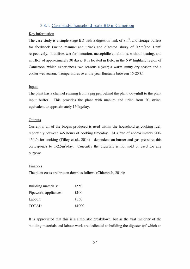
57

3.8.1. Case study: household-scale BD in Cameroon

Key information

The case study is a single-stage BD with a digestion tank of 8m3, and storage buffers

for feedstock (swine manure and urine) and digested slurry of 0.5m3and 1.5m3

respectively. It utilises wet fermentation, mesophilic conditions, without heating, and

an HRT of approximately 30 days. It is located in Belo, in the NW highland region of

Cameroon, which experiences two seasons a year; a warm sunny dry season and a

cooler wet season. Temperatures over the year fluctuate between 15-25ºC.

Inputs

The plant has a channel running from a pig pen behind the plant, downhill to the plant

input buffer. This provides the plant with manure and urine from 20 swine;

equivalent to approximately 150kg/day.

Outputs

Currently, all of the biogas produced is used within the household as cooking fuel;

reportedly between 4-5 hours of cooking time/day. At a rate of approximately 200-

450l/h for cooking (Tilley et al., 2014) - dependent on burner and gas pressure; this

corresponds to 1-2.5m3/day. Currently the digestate is not sold or used for any

purpose.

Finances

The plant costs are broken down as follows (Chiambah, 2014):

Building materials: £550

Pipework, appliances: £100

Labour: £350

TOTAL: £1000

It is appreciated that this is a simplistic breakdown, but as the vast majority of the

building materials and labour work are dedicated to building the digester (of which an

58

additional one will be required for our analysis), it was deemed to be sufficient. A

more detailed, itemised breakdown of costs can be found in Table 17 in Appendix 1.

The plant itself was built to reduce the need for firewood and the associated health

and environmental problems which come with it. Prior to cooking on biogas, this

household spent approximately £20 on firewood/month. Capital investment of £1000,

divided by £20 gives a payback period of 50 months - just over 4 years (Chiambah,

2014).

If the biogas yield improves with the addition of components, then there will simply

be more biogas available to the household; payback period will not improve unless

biogas is sold - either by piping it to a neighbour or compressing and bottling it - or an

electricity generator is fitted and savings made to the household electricity bill, or

energy exported.

As such plants are frequently in operation in areas where there is no electric network,

considering electricity was out of the scope of this study. Selling the additional

biogas via pipeline shall be explored instead; from the financial breakdown, pipework

and appliances cost £100. It can be reasonably assumed that a similar cost will be

incurred to pipe gas to a neighbour.

3.8.2. Removal of non-essential components

The following components needed to be removed from the tool in order to model a

household-scale BD:

• Reception tank mixer

• Input buffer tank mixer

• Digestate mixer

• 1st and 2nd stage digester mixers

• Primary and secondary shredders

• 2nd stage digester

• Reception tank discharge pump

59

• Pasteurisation mixer

• Pasteuriser

• Input buffer tank discharge pump

• Pasteurisation discharge pump

• 1st and 2nd stage digester discharge pumps

• Heat exchanger 1 (exit from 2nd stage digester)

• Heat exchanger 2 (exit from pasteuriser)

• Heat exchanger 3 (exit from engine coolant)

• Bio filter air fan

• Gas holder air fan

• CHP gas engine

• Heating for 1st and 2nd stage digesters

Dis-enabling the pasteuriser and second-stage digester was done by setting their HRTs

to zero i.e. the feedstocks were not considered to pass through the components.

The remainder of the components are only considered by the tool in order to calculate

their energy requirements; they were therefore set to zero.

3.8.3. Addition of components

The addition of components had to be performed in a systematic way so that the

effects of adding a component could be easily seen. The same three components –

input buffer, digester, and output buffer – were always present in the analysis, and the

other components – digester 2, shredder and heating (different levels) – were

systematically added, whilst recording the corresponding changes in performance and

cost. Mixers were not added as they were no suitable factor was found by which they

could be deemed to improve methane yield (see section 3.4.3), and they would only

serve to increase cost with no benefit. These combinations are shown in a matrix (see

Table 12). This shows all the possible combinations of additions of components

added to the original system.

60

As the ambient temperature is 15-25ºC, it was decided that digestion should take

place at the mean temperature of 20ºC. Where heating was used, 3 separate heating

temperatures were chosen; 25, 30 and 35ºC. It is appreciated that modelling over a

year using weather data for ambient temperature would provide more accurate results,

but is outwith the scope of this study.

Table 12 - Matrix showing combinations of components

Component

System name Digester 1 Digester 2 Heating Temp. (oC) Shredder

1 x x

2.1 x

25

2.2 x

30

2.3 x

35

3 x

x

4.1 x x 25

4.2 x x 30

4.3 x x 35

5 x x

x

6.1 x

25 x

6.2 x

30 x

6.3 x

35 x

7.1 x x 25 x

7.2 x x 30 x

7.3 x x 35 x

As a check that the tool is valid for the analysis of a small-scale system, the details for

the system as it stands were input; this gave a daily biogas output of 1.3-1.8m3/day;

within the estimates (based on 4-5 hours cooking time/day and 200-450l/h for

cooking) for actual production of 1-2.5 m3/day.

61

3.8.4. Costing of components

As discussed in section 3.5.1 above, the additional cost of a second digester would

simply be the same as the original digester, as they are identical. In this case study,

this would be £550. However, the costs of heating and shredders were not quantified;

in section 3.5 it was decided that due to the large range of solutions available, they

should be evaluated on a case by case basis.

Shredder

For this plant, processing 150kg of swine manure/urine per day, it was deemed most

appropriate to equate this feedstock to sludge, which is similar in moisture content

and biogas production potential. Ideally, a range of studies analysing this feedstock

would have been analysed, and the most appropriate shredder chosen and costed.

However, whilst there is a range of information on pre-treatment of feedstock, and the

effect upon biogas yield (amongst other factors), cost information is extremely

limited. Müller (2001) states that “The evaluation of capital and operational costs is

difficult, because of the lack of full-scale experience”, but gives a rough estimate of

between $70-150 USD/ton for capital and operation and maintenance costs. This was

the only data available on the subject of cost, and as it considered only larger scale,

was deemed insufficient for the purposes of cost analysis.

Heating

For heating methods, a document compiled by MinErgy Pvt. Ltd. (2014) was

consulted; this group has vast experience working with the type of BD used for the

case study – indeed, the BD used in Cameroon is based on the design used in Nepal,

of which there are over 280,000 built and in operation (BSP Nepal, 2012).

The recommendation from this document was a solar-powered heater, using water

which is then pumped through the BD to heat the substrate to the required

temperature. A schematic of the recommended system is shown in Figure 6.

62

Figure 6 - Schematic of solar-heated BD (MinErgy Pvt. Ltd., 2014)

Again, however, costs were unavailable. It was therefore decided that the model be

altered slightly; rather than making comparisons between yield improvement and cost

increase, a boundary was set so that a maximum acceptable cost increase could be

determined.

The payback period for the plant as it stands is currently 4 years (approximately). It

was decided to analyse a range of acceptable payback periods; increases of 25, 50, 75

and 100% (i.e. 4 years to 5, 6, 7 and 8 years respectively) were set. In evaluating the

maximum acceptable investment, the following was used:

6��� � �&7��� �&� = 5 " ����%��&8� � * 1000

Where

$���%��&8� � � £20��� �&�� " 12 " ���%��&8����������

If an addition to the plant caused biogas yield to improve and the associated cost

increase meant that the payback period was acceptable, then the additional

component(s) could be considered a success and be recommended.

63

4. Results

4.1. Variation in Performance

The performance and financial details for the original system are shown in Table 13.

When components were added to the system, improvements in biogas production

were recorded as shown in Table 14. This compares the 7 possible systems (15

configurations in all when different heating regimes are considered) with the original

system. It shows that with the addition of a singular component, it would appear that

adding heating would improve yield the most. A shredder is the second most

advantageous addition and a second digester the least.

Table 13 - Performance and financial details for original system

Income/year (£) Biogas yield (m3

/day) Capital cost (£) Payback period (years)

240 1-2.5 1000 4.16

Again, when two components are added, it is always the combination including

heating that improves yield the most. Therefore, if heating is comparable in price to

either a shredder or a second digester, its addition should be prioritised.

When using all three components, it is clear that the best results are achieved when

heating at higher temperatures. The performance variability factors in Table 7

(derived in section 3.6) are factors by which to scale up biogas yield and as such these

results are to be expected. It is when analysed in combination with the maximum

allowable investment that they become more interesting.

64

Table 14 - Yield improvements for all systems

System Yield improvement (%)

1 - Second digester 11.7

2.1 - Heating at 25oC 22

2.2 - Heating at 30oC 44

2.3 - Heating at 35oC 66

3 - Shredder 38

4.1 - Second digester, heating at 25oC 54

4.2 - Second digester, heating at 30oC 61

4.3 - Second digester, heating at 35oC 85

5 - Second digester, shredder 54

6.1 - Shredder, heating at 25oC 68

6.2 - Shredder, heating at 30oC 99

6.3 - Shredder, heating at 35oC 129

7.1 - Second digester, shredder, heating at 25oC 88

7.2 - Second digester, shredder, heating at 30oC 122

7.3 - Second digester, shredder, heating at 35oC 156

4.2. Maximum Allowable Investment

Evaluating maximum allowable investment using the formula derived in section 3.8.4,

Table 15 was gained for a 5 year payback period; Table 16 compares this with 6, 7

and 8 year payback periods. Note that the maximum investment covers initial

investment and maintenance costs, as well £100 for a pipeline to supply and sell

biogas to a neighbour – assumed to be sold at the same value the household is

presently gaining through firewood savings.

65

Table 15 - Maximum investment possible with 5 year payback period

Maximum Acceptable Investment for a 5 Year Payback Period

System Income/year (£) Maximum investment (£)

1 - Second digester 268.08 340.4

2.1 - Heating at 25oC 292.8 464

2.2 - Heating at 30oC 345.6 728

2.3 - Heating at 35oC 398.4 992

3 - Shredder 331.2 656

4.1 - Second digester, heating at 25oC 369.6 848

4.2 - Second digester, heating at 30oC 386.4 932

4.3 - Second digester, heating at 35oC 444 1220

5 - Second digester, shredder 369.6 848

6.1 - Shredder, heating at 25oC 403.2 1016

6.2 - Shredder, heating at 30oC 477.6 1388

6.3 - Shredder, heating at 35oC 549.6 1748

7.1 - Second digester, shredder, heating at 25oC 451.2 1256

7.2 - Second digester, shredder, heating at 30oC 532.8 1664

7.3 - Second digester, shredder, heating at 35oC 614.4 2072

66

Table 16 - Maximum investment possible with 5, 6, 7 and 8 year payback periods

Maximum Acceptable Investment (£) with Payback Period

System 5 year payback

period

6 year payback

period

7 year payback

period

8 year payback

period

1 340.4 608.48 876.56 1144.64

2.1 464 756.8 1049.6 1342.4

2.2 728 1073.6 1419.2 1764.8

2.3 992 1390.4 1788.8 2187.2

3 656 987.2 1318.4 1649.6

4.1 848 1217.6 1587.2 1956.8

4.2 932 1318.4 1704.8 2091.2

4.3 1220 1664 2108 2552

5 848 1217.6 1587.2 1956.8

6.1 1016 1419.2 1822.4 2225.6

6.2 1388 1865.6 2343.2 2820.8

6.3 1748 2297.6 2847.2 3396.8

7.1 1256 1707.2 2158.4 2609.6

7.2 1664 2196.8 2729.6 3262.4

7.3 2072 2686.4 3300.8 3915.2

67

4.3. Summary of Results

Tables 14, 15 and 16 show the following:

System 1 – Second digester

Adding a second digester to the system increased biogas production by 11.7%.

Maximum possible investment was £340.40, £608.48, £876.56 and £1144.64 for 5, 6,

7 and 8 year payback periods respectively.

System 2 – Heating

Heating the original system to 25 ºC increased yield by 22%. Maximum possible

investment was £464, £756.80, £1049.60 and £1342.40 for 5, 6, 7 and 8 year payback

periods respectively.

Heating to 30 ºC increased yield by 44% - allowable investment increased to £728,

£1073.60, £1419.20 and £1764.80 for 5, 6, 7 and 8 year payback periods respectively,

whilst heating to 35ºC yielded 66% more biogas than the original system with an

allowable investment of £992, £1390.40, £1788.80 and £2187.20 for 5, 6, 7 and 8

year payback periods respectively.

System 3 – Shredder

Adding a shredder to the original system led to a 38% improvement in yield, with

allowable investment thresholds of £656, £987.20, £1318.40 and £1649.60 for 5, 6, 7

and 8 year payback periods respectively.

System 4 – Second digester and heating

Adding a second digester and heating to 25ºC improved yield by 54%. Maximum

possible investment was £848, £1217.60, £1587.20 and £1956.80 for payback periods

of 5, 6, 7 and 8 years respectively.

Adding a second digester and heating to 30ºC improved yield by 61%. Maximum

possible investment was £932, £1318.40, £1704.80 and £ 2091.20 for payback periods

of 5, 6, 7 and 8 years respectively.

68

Adding a second digester and heating to 35ºC improved yield by 85%. Maximum

possible investment was £1220, £1664, £2108 and £2552 for payback periods of 5, 6,

7 and 8 years respectively.

System 5 - Second digester and shredder

Adding a second digester and a shredder to the original system led to a 54% increase

in yield, with maximum possible investment values of £848, £1217.60, £1587.20 and

£1956.80 for payback periods of 5, 6, 7, and 8 years respectively.

System 6 – Shredder and heating

Adding a shredder and heating to 25ºC improved yield by 68%. Maximum possible

investment was £1016, £1419.20, £1822.40 and £2225.60 for payback periods of 5, 6,

7 and 8 years respectively.

Adding a shredder and heating to 30ºC improved yield by 99%. Maximum possible

investment was £1388, £1865.60, £2343.20 and £2820.80 for payback periods of 5, 6,

7 and 8 years respectively.

Adding a shredder and heating to 35ºC improved yield by 129%. Maximum possible

investment was £1748, £2297.60, £2847.20 and £3396.80 for payback periods of 5, 6,

7 and 8 years respectively.

System 7 – Second digester, shredder and heating

Adding a second digester, shredder and heating to 25ºC improved yield by 88%.

Maximum possible investment was £1256, £1707.20, £2158.40 and £2609.60 for

payback periods of 5, 6, 7 and 8 years respectively.

Adding a second digester, shredder and heating to 30ºC improved yield by 122%.

Maximum possible investment was £1664, £2196.80, £2729.60 and £3262.40 for

payback periods of 5, 6, 7 and 8 years respectively.

Adding a second digester, shredder and heating to 35ºC improved yield by 156%.

Maximum possible investment was £2072, £ 2686.40, £3300.80 and £3915.20 for

payback periods of 5, 6, 7 and 8 years respectively.

69

4.4. Discussion of Results

Comparing systems with a single additions; i.e. systems 1, 2 and 3 it can be seen that

heating to 30ºC or above provided the largest yield improvement, followed by the

addition of a shredder (which had a comparable yield improvement to heating to

30ºC), with the addition of a second digester giving the least yield improvement.

Whilst costs are unknown, a shredder would likely cost less than £656 which is the

maximum possible investment with a 5 year payback period.

The cost of a second digester would be £550, plus £100 for a pipeline connection to a

neighbour – over the acceptable limit of £340.40, so this investment does not seem

worthwhile with a 5 year payback period. However, is has been shown to be a viable

option if an acceptable payback period for a BD is set at 6 years – this may be an

option for households which require larger quantities of gas (and may have larger

incomes due to size).

Considering heating, whilst it is clear that heating to a higher temperature yields more

biogas, it is not obvious which heating regime would be the most viable, and thus

further work is required in costing such systems.

Comparing systems with two additions; i.e. systems 4, 5 and 6 it can be seen that the

systems using heating have the highest biogas yields; the most advantageous system is

system 6, which utilises heating in addition to a shredder (yield improvements 68-

129%). The second best system here uses a second digester and heating (yield

improvements 54-85%), followed by a second digester and shredder (yield

improvement of 54%).

As it is likely that a shredder would cost less than a second digester (£550), if heating

is to be used in conjunction with another component, a shredder should be given

priority over using a second digester.

System 7, which utilises heating, a second digester and a shredder, shows a yield

improvement from 88-156%. This top-end figure is the highest yield improvement

found. Interestingly, systems 7 and 6 overlap in yield improvement, and a careful

70

analysis of cost vs. yield would have to be undertaken system 7 were to be

considered; it may be that system 6 is more financially viable.

These results show that appreciable gains in biogas yield can be made with little

modification to a small-scale household BD. Further work is required to fully cost

heating and shredding systems in order to verify their viability for investment in the

short-term for small-scale household plants.

Large scale plants tend to have a longer lifespan, and hence payback periods than

small-scale BDs - in the region of 20 years. It is partially due to this that generally,

only large-scale plants operate with a second digester, heating and shredders. In

addition to this, a large scale plant will have a far higher output of biogas and so

maximum possible investment in these components would increase accordingly.

If this 20 year lifespan were applied to a small-scale BD, then the maximum

investment would be £4360 for a second digester, £4856, £5912 and £6968 for

heating at 25, 30 and 35 ºC respectively and £5624 for a shredder. Using all three

systems in combination, heating to 35 ºC, would allow an investment of £11288.

Whilst costs are currently unknown for heating and shredding systems, it can be

appreciated that they would be likely affordable with a 20 year payback period.

However, in a developing country, 20 years is a relatively long time. In Cameroon,

where the average life expectancy is 55 (World Bank, 2015), such an investment

would not be deemed worthwhile. Payback period of a plant, and cost, is a huge

driver behind the technology of small-scale BDs; we have just shown that with a 6

year payback period, a second digester is a viable option – yet the majority of these

plants only incorporate one. Designers possibly deemed such an investment

unattractive to potential end users, thus discounting it.

71

4.5. Recommendations

Reviewing the above results, the following recommendations can be made:

• If a payback period of 6 years is set, then a second digester is a viable option

• Whilst costs of heating systems are unknown, they have the highest impact on

biogas yield. It is therefore recommended that the greatest investment be put

into heating systems

• Heating at 25, 30 and 35ºC increased yield by 22, 44 and 66%; clearly

showing that heat has a considerable impact on biogas yield and that higher

temperatures give far higher biogas yields. It is likely that a system which

would provide 25ºC heat would be the same as a system which would provide

35ºC heat. It is therefore recommended that if such a system is installed, it be

run at the optimal temperature for the specific substrate (as opposed to a lower

temperature to save on bills).

• Heating should be used if ambient temperature is less than 15°C

• If an improvement using two components and including heating is to be

considered, the addition of a shredder should take priority over a second

digester

• Finances are clearly quite tight for such a small-scale BD, which only gains

profit through solid fuel savings. It is therefore recommended that a market

for the digestate be found to increase profit and reduce payback period.

72

5. Conclusions and Future Work

It was recognised that BDs have the potential to reduce greenhouse gas emissions

through burning methane, rather than allowing it to escape into the atmosphere. In

addition, they reduce the need for firewood to be burned, releasing carbon dioxide and

contributing to deforestation.

Whilst large-scale plants are gaining in popularity in more developed countries, they

are less accessible in developing countries due to cost limitations; the aim of this

study was therefore to explore ways in which small-scale plants could become more

profitable, with minimal additional investment. To do this, a literature review was

conducted to determine the best computational method to use to model a small-scale

BD.

Once a suitable tool was found, it was analysed for components modelled, to discover

which were pertinent to biogas yield. Another literature review was undertaken to

determine how these particular components affected performance (biogas yield) and

financial viability.

It was found that adding an additional digester improved biogas yield by 17.7% (a

mean value taken from 5 studies). It was recognised that for further accuracy, specific

substrates would have to be examined so that substrate-specific values could be

programmed into the tool. Additionally, where information lacked, lab work could be

undertaken – these measures were, however, outwith the scope of this study.

An additional digester would increase the cost by £38.20 x the original digester

volume – this again was an average value from studies examined.

To examine heating, values for a range of studies examining the effects of heating

were plotted on a graph, and an r2 average value for the biogas yield increase over

time was obtained. As the tool calculated yield based on a temperature of 35ºC, this

formula was used to decrease yield at temperatures below 35ºC, and increase yield at

temperatures above 35ºC (between 20ºC to 45ºC, as these are the limiting

temperatures of bacteria operating within a mesophilic BD). The cost increase for

73

heating was taken as the reduction in available gas (if a gas heater is used) plus the

initial capital required.

Studies for mixers were inconclusive and thus no yield or financial factors were

derived; shredders were found to provide a mean yield improvement of 27.6%, and

cost was to be evaluated on a case by case basis.

The performance variability factors were then used to alter biogas yield if their

relevant component was present in the system, and the financial variability factors

were built into a new “Financial Viability” section.

Once the tool had been altered, it had to be validated. For this, data for an existing

plant in Lelbach, Germany was used. This plant was modelled, and it was decided

that outputs from the tool would have to be within 50% of actual data for the tool to

be deemed valid. The tool showed reasonable levels of accuracy in estimating biogas

and electricity output – overestimating by 33% and 11% respectively - but not in heat

output – overestimating by 105%. This discrepancy was likely down to differences in

the CHP engines used, and was considered acceptable as heat output was not a focus

of this study.

Once the tool had been validated, it had to be altered so that it was suitable to model a

case study of a small-scale household BD in Belo, Cameroon. This was done by

“stripping back” the tool so that only the three components used in the small-scale

case study were present; input buffer, digester and output buffer. This was done by

reducing the HRT time of the pasteuriser and second digester, as well as the electrical

requirements of all other components to zero.

Once this was completed, the components pertinent to biogas production (additional

digester, shredder and heating at 25, 30 and 35ºC) were modelled in every

combination possible – 15 in all – to analyse their impact upon biogas yield and

financial viability.

74

It was found that heating provided the highest increase in yield, followed by a

shredder and with the addition of a second digester. For combinations of two

components, heating in combination with a shredder appeared to be the best option,

and for all three components, highest yield was gained by heating at higher

temperatures.

It was therefore recommended that solutions for low-cost heating be found, and

secondarily, shredders. The cost of a second digester was already known so it was

recommended that with an acceptable payback period of 6 years or more, a second

digester be used. It was also noted that a driver for cost was acceptable payback

period, which in developing countries can be very tight; this led to the

recommendation that ways to ease this be explored, such as additional revenue from

the plant.

During the course of this research, it became apparent that the following areas could

provide useful and insightful research avenues:

• The literature review uncovered very few software-based tools available which

could be used to model BDs. There is scope to develop this tool further, or

create a new tool based on findings in this report - if made freely available

this could encourage potential future investors and could provide a boost to the

BD industry

• It was acknowledged that the performance variability factors could have been

more accurate. This could have been done by deriving substrate, system and

temperature specific factors for each component, from a very wide ranging

literature review, or from laboratory work. Built into the tool, this would

improve the accuracy enormously

• Climate data could be built into the tool, to model a BD over a year as the

ambient temperature fluctuates and biogas production is affected if the BD is

unheated. If heated, the heating requirement could be calculated over the year

with greater accuracy

75

• The tool did not take into account dynamic effects e.g. the heat available to the

digesters is dependent on the gas available which is dependent on the heat of

the digesters. Such effects could be included for greater accuracy

• A literature review revealed a scarcity of information on the subject of low-

cost heating and insulation systems – research into which could provide

invaluable to end-users of BDs in cooler climates.

• Additionally, whilst the impacts of mechanical pre-treatment has been

reasonably well-documented, it would appear that such systems are only

available to large-scale plant; any research done on a small scale is conducted

using lab equipment. Research and development in this field could prove a

useful exercise, as it has already been shown that mechanical pre-treatment

can have a substantial effect on biogas yield

• The major driver behind the acceptability of investment costs appears to be

payback period. This is due to plant lifetime, and also the fact that people in

developing countries find long payback periods unfeasible. Ways to improve

the acceptability of payback period increases should be explored – potentially

through improvements in plant robustness, co-operative/community BDs, and

additional ways to make income from the plant, such as selling the digestate as

fertiliser

76

6. Appendix I – Small-Scale Case Study Plant Details

Table 17 - Cost breakdown for small-scale BD case study

77

Figure 7 - General biogas plant drawing, design for small scale BD case study (BSP

Nepal, 2015

78

Table 18 - Dimensions for Figure 7 (BSP Nepal, 2015)

79

7. References

Abdel-Hadi, M.A., Abd El-Azeem, S.A.M., 2008. Effect of heating, mixing and

digester type on biogas production from buffalo dung. Misr Journal of Agricultural

Engineering, Vol. 25(4), pp. 1454–1477.

Alkhamis, T.M., El-khazali, R., Kablan, M.M., Alhusein M.A., 2000. Heating of a

biogas reactor using a solar energy system with temperature control unit. Solar

Energy, Vol. 69(3), pp. 239–247.

Angelidaki, I., Ellegaard, L., Ahring, B.K., 2000. A comprehensive model of

anaerobic bioconversion of complex substrates to biogas. Biotechnology and

Bioengineering, Vol. 63(3), pp. 363–372.

Arora, K., 2015. Calibrating Slurry Tank Manure Applicators.

https://www.extension.iastate.edu/Pages/communications/EPC/Fall03/slurrytank.html

Accessed 21/08/2015

Arikan, O.A., Mulbry, W., Lansing, S., 2015. Effect of temperature on methane

production from field-scale anaerobic digesters treating dairy manure. Waste

Management, Vol. 43, pp. 108–113.

Baier, U., Schmidheiny, P., 1997. Enhanced anaerobic degradation of mechanically

disintegrated sludge. Water Science and Technology, Vol. 36(11), pp. 137–114.

Barjenbruch, M., Kopplow, O., 2003. Enzymatic, mechanical and thermal pre-

treatment of surplus sludge. Advances in Environmental Research, Vol. 7(3), pp.

715–720.

80

Cenex, 2009. Biomethane Toolkit - A guide to the production and use of biomethane

as a road transport fuel (Online). Available at

https://www.americanbiogascouncil.org/pdf/Cenex-biomethane-toolkit-2009.pdf,

accessed 24/08/2015.

Colorado State University, 2015. Anaerobic Digestion Feasibility Tool (Online).

Available at https://erams.com/ad_feasibility_ad_tool/, accessed 24/08/2015

Chiambah, E., 2014. Biogas Demonstration Site to Educate the Belo Community in

the Highlands of the North West Region of Cameroon. Proposal for Belo Rural

Development Association (BERUDA), P.O. Box 22, Njinikom, Boyo Division

North West Region, Bamenda, Cameroon

Bouallagui, H., Haouari, O., Touhami, Y., Cheikh, R.B., Marouani, L., Hamdi, M.,

2004. Effect of temperature on the performance of an anaerobic tubular reactor

treating fruit and vegetable waste. Process Biochemistry, Vol. 39(12), pp. 2143–

2148.

Bond, T. and Templeton, M.R., 2011. History and future of domestic biogas plants in

the developing world. Energy for Sustainable Development, Vol. 15(4), pp. 347–354.

BSP (Biogas Support Programme) Nepal, 2012. Interim Phase Year Book.

http://www.bspnepal.org.np/docs/publication/year_book_2012.pdf, Accessed

10/07/2015

BSP (Biogas Support Programme) Nepal, 2015 (Online). Available at

http://www.bspnepal.org.np/?option=cms&cid=16, accessed 22/08/2015

BPEX, 2010. Added Value from Pig Manure and Slurries (Online). Available at

http://pork.ahdb.org.uk/media/2261/added_value_from_pig_manures_and_slurries.pd

f, accessed 17/07/2015

81

Chen, T.H., Chynoweth, P., BIljetina, R., 1990. Anaerobic digestion of municipal

solid waste in a nonmixed solids concentrating digester. Applied Biochemistry and

Biotechnology, Vol. 24–25(1), pp.533–544.

Dachs, G., Rehm, W., 2006. Der Eigenstromverbrauch von Biogasanlagen und

Potenziale zu dessen Reduzierung. Germany: Hg. v. Solarenergieförderverein

Bayern e.V. München (Online). Available at https://www.sev-bayern.de/content/bio-

eigen.pdf, accessed 05/08/2015

Callaghan, F.J., Wase, D.A.J., Thayanithy, K., Forster, C.F, 1998. Co-digestion of

waste organic solids: batch studies. Bioresource Technology, Volume 67(2), pp.

117-122.

Carrère, H., Dumas, C., Battimelli, A., Batstone, D.J., Delgenès, J.P., Steyer, J.P.,

Ferrer, I. 2010. Pre-treatment methods to improve sludge anaerobic degradability: A

review. Journal of Hazardous Materials, Volume 183(1–3), pp. 1-15

Chae, K. J., Jang, A., Yim, S. K., Kim, I.S., 2008. The effects of

digestion temperature and temperature shock on the biogas yields from

the mesophilic anaerobic digestion of swine manure. Bioresource Technology

Vol. 99(1), pp 1–6.

European Commission, 2014. Quarterly Report on European Electricity Markets.

Market Observatory for Energy, DG Energy, Volume 7 (3; third quarter of 2014).

Engelhart, M., Krger, M., Kopp, J., Dichtl, N., 2000. Effects of disintegration on

anaerobic degradation of sewage excess sludge in downflow stationary fixed film

digesters. Water Science and Technology, Vol. 41(3), pp. 171–179.

Ezzati, M. and Kammen, D.M., 2001. Quantifying the Effects of Exposure to Indoor

Air Pollution from Biomass Combustion on Acute Respiratory Infections in

Developing Countries. Environmental Health Perspectives, Vol. 109(5), pp. 481-488.

82

Flessa, H., Ruser, R., Dörsch, P., Kamp, T., Jimenez, M.A., Munch, J.C. Beese, F.,

2002. Integrated evaluation of greenhouse gas emissions (CO2, CH4, N2O) from two

farming systems in southern Germany. Agriculture, Ecosystems and Environment,

Vol. 91(1-3), pp. 175–189.

Forest Fuels, 2015. Fuel price comparisons (Online). Available at

http://www.forestfuels.co.uk/about-wood-fuel/fuel-price-comparisons, accessed

21/07/2015

Forest Power, 2015. Density of wet wood and loose density of wood chips (Online).

Available at

http://www.forestpower.net/data/liitteet/11620=1017_density_of_wet_wood.pdf,

accessed 21/07/2015

Forestry Commission Scotland, 2011. Woodchip Drying. Technical Development

Report reference FCPR045 (Online). Available at

http://www.biomassenergycentre.org.uk/pls/portal/docs/PAGE/RESOURCES/REF_L

IB_RES/PUBLICATIONS/TECHNICAL_DEVELOPMENT/FCPR045%20WOODC

HIP%20DRYING.PDF, accessed 15/07/2015

Gautam, R., Baral, S., Herat, S., 2007. Biogas as a sustainable energy source in

Nepal: Present status and future challenges. Renewable and Sustainable Energy

Reviews, Vol 13(1), pp. 248–252.

Geraghty, M., Roscoe, A.J., Cloonan, M., Currie, J., (2004). Biomass - Using

Anaerobic Digestion. (Online). Available at

http://www.esru.strath.ac.uk/EandE/Web_sites/03-04/biomass//index.html, accessed

15/05/2015.

Gibbons, J.M., Ramsden, S.J., Blake, A., 2006. Modelling uncertainty in greenhouse

gas emissions from UK agriculture at the farm level. Agriculture, Ecosystems and

Environment, Vol 112(4), pp. 347–355.

83

Hahn, H., Rutz, D., Ferber, E., Kirchmayer, F., 2010. Examples for financing of

biogas projects in Germany, Austria, The Netherlands, Denmark and Italy. Report

for IEE Project ‘BiogasIN’ (Online). Available at

http://www.biogasin.org/files/pdf/Financing_of_biogas_projects_in_top_5_EU_count

ries.pdf, Accessed 05/08/2015

Hahn, H., 2011. Guideline for financing agricultural biogas projects - Training

material for biogas investors. Report for IEE Project ‘BiogasIN’ (Online). Available

at http://www.biogasin.org/files/pdf/WP3/D.3.5_IWES_EN.pdf, accessed 05/08/2015

Hashimoto, A.G., 1982. Effect of mixing duration and vacuum on methane

production rate from beef cattle waste. Biotechnology and Bioengineering, Vol.

24(1), pp. 9-23.

He, P.J., 2010. Anaerobic digestion: An intriguing long history in China. Waste

Management, Vol. 30(4), pp. 549–550

Ho, C.C., Tan, Y.K., 1985. Anaerobic treatment of palm oil mill effluent by tank

digesters. Journal of Chemical Technology and Biotechnology, Vol. 35(2), pp. 155–

164.

IEA, 2002. World Energy Outlook (Online). Available at

http://www.worldenergyoutlook.org/media/weowebsite/2008-

1994/weo2002_part1.pdf, accessed 01/06/2015

IEA, 2014. Bioenergy Task 37 - Country Reports Summary (Online). Available at

http://www.ieabioenergy.com/wp-content/uploads/2015/01/IEA-Bioenergy-Task-37-

Country-Report-Summary-2014_Final.pdf, accessed 10/07/2015

IEA, 2015. Energy and Climate Change: World Energy Outlook Special Report

(Online). Available at

https://www.iea.org/publications/freepublications/publication/WEO2015SpecialRepor

tonEnergyandClimateChange.pdf, accessed 01/08/2015

84

INFORSE – Europe, 2006. Guideline for Estimation of Renewable Energy Potentials,

Barriers and Effects (Online). Available at http://www.inforse.org/europe/pdfs/RE-

asses-06.pdf, accessed 23/07/2015

IPCC, 2001. Climate Change: The Scientific Basis (Online). Available at

http://www.grida.no/climate/ipcc_tar/wg1/pdf/wg1_tar-front.pdf, accessed

15/08/2015

ISAT (Information and Advisory Services on Appropriate Technology), 1999. Biogas

Digest Volume I; Biogas Basics (Online). Available at

http://www.sswm.info/sites/default/files/reference_attachments/ISAT%20GTZ%2019

99%20Biogas%20digest%20Volume%20I%20Biogas%20Basics.pdf, accessed

18/08/2015

ISAT (Information and Advisory Service on Appropriate Technology), 2015. Biogas

Digest Volume III; Biogas - Costs and Benefits and Biogas – Programme

Implementation. (Online). Available at

http://www.sswm.info/sites/default/files/reference_attachments/GTZ%20ISAT%2019

99%20Biogas%20Digest%20Vol%203.pdf, accessed 10/08/2015.

ISO 6976 (1995) Natural gas - Calculation of calorific values, density, relative density

and Wobbe index from composition

James, S.C., Wiles, C.C., Swartzbauch, J.T., Smith, R.B., 1980. Mixing in large-scale

municipal solid waste sewage sludge. Biotechnology and Bioengineering, Vol. 22

(SI) pp. 259–272.

Kaltschmitt, M., Hartmann, H., Hofbauer, H., 2009. Energie aus biomasse. 2nd ed.

Berlin, Heidelberg: Springer.

Karellas, S., Boukis, I., Kontopoulos, G. 2010. Development of an investment

decision tool for biogas production from agricultural waste. Renewable and

Sustainable Energy Reviews, Vol. 14(4), pp. 1273–1282.

85

Karim, K., Hoffmann, R., Klasson, K.T., Al-Dahhan, M.H., September 2005.

Anaerobic digestion of animal waste: Effect of mode of mixing. Water Research, Vol.

39(15), pp. 3597–3606.

Karim, K., Hoffmann, R., Klasson, K.T., Al-Dahhan, M.H., November 2005.

Anaerobic digestion of animal waste: Waste strength versus impact of mixing.

Bioresource Technology, Vol. 96(16), pp. 1771-1781.

KTBL, 2015. Online European Feedstock Atlas Basic Version (Online). Available

at http://daten.ktbl.de/euagrobiogasbasis/navigation.do?selectedAction=Startseite,

accessed 16/17/2015.

Lang. M., and Lang, A., 2015. The 2014 German Renewable Energy Sources Act

revision – from feed in tariffs to direct marketing to competitive bidding. Journal of

Energy & Natural Resources Law, Vol. 33(2), pp. 131-146.

LEAD, 2006. Livestock’s Long Shadow. Environmental Issues and Options (Online).

Available at ftp://ftp.fao.org/docrep/fao/010/a0701e/a0701e.pdf, accessed 03/07/2015

Liu, D., Liu, D., Zeng, R.J., Angelidaki, I., 2006. Hydrogen and methane production

from household solid waste in the two-stage fermentation process. Water Research,

Vol. 40(11), pp. 2230-2236.

Lohri, C.R., Rodic, L., Zurbrügg, C., 2013. Feasibility assessment tool for urban

anaerobic digestion in developing countries. Journal of Environmental Management,

Vol. 126(15), pp. 122–131.

Luo, G., Xie, L., Zhou, Q., Angelidaki, I., 2011. Enhancement of bioenergy

production from organic wastes by two-stage anaerobic hydrogen and methane

production process. Bioresource Technology, Vol. 102(18), pp. 8700-8706.

86

Maschinenring Waldeck-Frankenberg eV., 2015. Eckdaten SBW Biogas Lelbach

(Online). Available at http://www.mr-wa-fkb.de/erneuerbare_energien/biogas-

erzeugung/.eckdaten_lelbach.html, accessed 24/08/2015

Maspolim, Y., Zhou, Y., Guo, C., Xiao, K., Ng, W.J., 2014. Comparison of single-

stage and two-phase anaerobic sludge digestion systems – Performance and

microbial community dynamics. Chemosphere, Vol. 140, pp. 54–62.

Methanogen ltd., 2010; Report prepared for The Peak District National Park Authority

and East Midlands Development Agency. A Toolbox Guide for Assessing the

Feasibility of an Anaerobic Digestion Project Developed for the Benefit of a

Community or for a Single Farm (Online). Available at http://www.r-e-

a.net/upload/toolkit_-_david_collins_community_biogas.pdf, accessed 24/08/2015

MinErgy Pvt. Ltd., Nepal. 2014. Optimization of Biogas Plants using Digester

Heating Technologies. Submitted to Biogas Sub Component National Rural and

Renewable Energy Programme (NRREP), Alternative Energy Promotion Center

(AEPC) Khumaltar, Lalitpur, Nepal (Online). Available at

http://www.aepc.gov.np/docs/resource/subreport/20140708034742_Final%20Report_

Digester%20Heating.pdf, accessed 12/08/2015

Montgomery, L.F.R., Bochmann, G., 2014. Pre-treatment of feedstock for

enhanced biogas production. IEA Bioenergy, ISBN 978-1-910154-05-2.

Müller. J.A., 2001. Prospects and problems of sludge pre-treatment processes.

Water Science and Technology, Issue 44(10), pp. 121–128.

Nasr, N., Elbeshbishy, E., Hafez, H., Nakhla, G., El Naggar., M.H., 2012.

Comparative assessment of single-stage and two-stage anaerobic digestion for the

treatment of thin stillage. Bioresource Technology, Vol. 111, pp. 122-126.

Nijaguna, B.T., 2007. Biogas Technology. New Age International Pvt Ltd

Publishers, ISBN: 8122413803.

87

Olesen, J.E., Schelde, K., Weiske, A., Weisbjerg, M.R., Asman, W.A.H., Djurhuus,

J., 2006. Modelling greenhouse gas emissions from European conventional and

organic dairy farms. Agriculture, Ecosystems and Environment, Vol. 112(2-3), pp.

207–220

Ong, H., Greenfield, P., Pullammanappallil, P., 2002. Effect of mixing on

biomethanation of cattle-manure slurry. Environmental Technology, Vol. 23(10,) pp.

1081–1090.

Pakarinen, O.M., Tähti, H.P., Rintala, J.A., 2009. One-stage H2 and CH4 and two-

stage H2 + CH4 production from grass silage and from solid and liquid fractions of

NaOH pre-treated grass silage. Biomass and Bioenergy, Vol. 33(10), pp. 1419-1427.

Palmowski, L., Muller, J., 1999. Influence of the size reduction of organic waste on

their anaerobic digestion. In: Mata-Alvarez, J., Tilche, A., Cecchi, F. (Eds.),

Proceedings of the second international symposium on anaerobic digestion of

solid wastes, Barcelona, pp. 137-144.

Parkin, G.F., Owen, W.F., 1986. Fundamentals of anaerobic digestion of wastewater

sludges. J Environ Eng Vol. 112(5), pp. 867–920.

Regulation (EC) No 1069/2009, 2009. Laying down health rules as regards animal

by-products and derived products not intended for human consumption and repealing

Regulation (EC) No 1774/2002 (Animal by-products Regulation).

Road Haulage Association, 2006. Cost Tables (Online). Available at

https://www.rha.uk.net/docs/internet/operatingcosts/RHA%20Cost%20Tables.pdf,

accessed 10/07/2015.

Rogers, G., Mayhew, Y. 1992. Engineering Thermodynamics: Work and Heat

Transfer. Longman Scientific; 4th edition. ISBN: 0582045665

88

Safley Jr., L.M., Westerman, P.W., 1994. Low-temperature digestion of dairy and

swine manure. Bioresource Technology, Vol. 47(2), pp. 165-171.

Sasse L., 1998. Biogas Plants. A Publication of the Deutsches Zentrum für

Entwicklungstechnologien - GATE in: Deutsche Gesellschaft für Technische

Zusammenarbeit (GTZ) GmbH, Eschborn, Germany (Online). Available at

http://www.susana.org/_resources/documents/default/2-1799-biogasplants.pdf,

accessed 22/07/2015

Scheinberg, A., Wilson, D.C., Rodić, L., 2010. Solid Waste Management in the

World's Cities. UN-habitat's Third Global Report on the State of Water and Sanitation

in the World’s Cities. Earthscan for UN Habitat, London (Online). Available at

http://mirror.unhabitat.org/pmss/listItemDetails.aspx?publicationID=2918, accessed

24/08/2015

Schievano, A., Tenca, A., Scaglia, B., Merlino, G., Rizzi, A., Daffonchio, D., Oberti,

R., Adani, F., 2012. two-stage vs Single-Stage Thermophilic Anaerobic Digestion:

Comparison of Energy Production and Biodegradation Efficiencies. Environmental

Science and Technology, Vol. 46(15), pp. 8502–8510.

Schils, R.L.M., Verhagen, A., Aarts, H.F.M., Šebek, L.B.J., 2005. A farm level

approach to define successful mitigation strategies for GHG emissions from ruminant

livestock systems. Nutrient Cycling in Agroecosystems, Vol. 71, pp. 163–175.

Sharma, S.K., Mishra, I.M., Sharma, M.P., Saini, J.S., 1988. Effect of particle size on

biogas generation from biomass residues. Biomass, Vol. 17(4), pp. 251-263.

Sharma, S.K., Saini, J.S., Mishra, M., Sharma, M.E., 1989. Biogasification of woody

biomass: Ipomoea fistulosa plant stem. Biological Wastes, Vol. 28(1), pp 25-32.

Sharma, C.K., 1996. Overview of Nepal’s Energy Sources and Environment.

Atmospheric Environment, Vol. 30(15), pp. 2717-2720.

89

Song, Y.C., Kwon, S.J., Woo, J.H., 2004. Mesophilic and thermophilic temperature

co-phase anaerobic digestion compared with single-stage mesophilic- and

thermophilic digestion of sewage sludge. Water Research, Vol. 38(7), pp. 1653–1662.

Stenstrom, M.K., Ng, A.S., Bhunia, P.K., Abramson, S.D., 1983. Anaerobic

digestion on municipal solid waste. J Environ Eng 1983, Vol. 109(5), pp. 1148–1158.

TDBP (Tanzania Domestic Biogas Programme), 2015 (Online). Available at

http://www.biogas-tanzania.org/tdbp/about/category/archievements, accessed

26/07/2015

Tian, H., Duan, N., Lin, C., Li, X., and Zhong, M, 2014. Anaerobic co-digestion of

kitchen waste and pig manure with different mixing ratios. Journal of Bioscience and

Bioengineering, Vol. 120(1), pp. 51-57.

Tilley, E., Ulrich, L., Luethi, C., Reymond, P., Zurbruegg, C. 2014. Direct Use of

Biogas (Online). Available at http://www.sswm.info/content/direct-use-biogas,

accessed 19/08/2015

Troschinetz, A.M., Mihelcic, J.R., 2008. Sustainable recycling of municipal solid

waste in developing countries. Waste Management, Issue 29(2), pp. 915–923.

UNESCO, 2012. Education For All Global Monitoring Report; Youth and Skills –

Putting Education to Work (Online). Available at

http://unesco.nl/sites/default/files/dossier/2012_gmr.pdf?download=1, accessed

16/07/2015

Wang, Z., Chen, S., Frear, C., Kruger, C., Granatstein, D. 2009. Advanced small-

scale anaerobic digester design tailored for household user living in cold climate.

Washington State University, Pullman WA (WSU) and Biological and Environmental

Systems and Technologies, LLC, Pullman, WA (BEST).

90

Warwick, H. and Doig, A., 2004. Smoke – the Killer in the Kitchen: Indoor Air

Pollution in Developing Countries (Online). Available at

http://practicalaction.org/docs/smoke/itdg%20smoke%20report.pdf, accessed

10/07/2015

Wett, B., Phothilangka, P., Eladawy, A., 2010. Systematic comparison of mechanical

and thermal sludge disintegration technologies. Waste Management, Vol. 30(6), pp.

1057–1062.

Weiland, P., Biogas production: current state and perspectives., 2010. Applied

Microbiol Biotechnology, Vol. 85(4), pp. 849–860.

WHO, 2015. Indoor Air Pollution (Online). Available at

http://www.who.int/indoorair/en/, accessed 23/07/2015

Wiese, J., and Kujawski, O, 2008. Operational Results of an Agricultural Biogas

Plant Equipped with Modern Instrumentation and Automation. Water Science and

Technology, Vol. 57(6), pp. 803–808.

Wilson, D.C., Rodić, L., Scheinberg, A., Velis, C.A., Alabaster. G. 2012.

Comparative analysis of solid waste management in 20 cities. Waste Management

and Research, Vol. 30(3), pp. 237–254.

World Bank, 2015. Life expectancy at birth, total (Online). Available at

http://data.worldbank.org/indicator/SP.DYN.LE00.IN, accessed 22/08/2015.

Xe.com, 2015. Exchange rates. Available at www.xe.com, accessed29/07/2015