Routing Algorithms Analysis for Wireless Sensor Networks COEN 233 Team Project

Team 4: Yang Lei, Cong Peng & Min Xu

Table of Contents 1. Abstract ­­­­­­­­­­­­­­­­­­­­­­­­­­­­­­­­­­­­­­­­­­­­­­­­­­­­­­­­­­­­­­­­­­­­­­­­­­02 2. Introduction ­­­­­­­­­­­­­­­­­­­­­­­­­­­­­­­­­­­­­­­­­­­­­­­­­­­­­­­­­­­­­­­­­­­­­02 3. Theoretical Bases and Literature Review ­­­­­­­­­­­­­­­­­­­­­­­­­­­­­­­­­­­03 4. Hypothesis ­­­­­­­­­­­­­­­­­­­­­­­­­­­­­­­­­­­­­­­­­­­­­­­­­­­­­­­­­­­­­­­­­­­­­­­05 5. Methodology ­­­­­­­­­­­­­­­­­­­­­­­­­­­­­­­­­­­­­­­­­­­­­­­­­­­­­­­­­­­­­­­­­­­­05

5.1 Methodology for Multipath Routing ­­­­­­­­­­­­­­­­­­­­­­­­­­­­­05 5.2 Methodology for Localized Single­Path Routing Topology

Generation ­­­­­­­­­­­­­­­­­­­­­­­­­­­­­­­­­­­­­­­­­­­­­­­­­­­­­­­­­­­­­­­­07 5.2.1 Single­path Routing Topology Generation and Metric

Calculation ­­­­­­­­­­­­­­­­­­­­­­­­­­­­­­­­­­­­­­­­­­­­­­­­­­­­­­­­07 5.2.2 Routing Topology Generation Algorithms ­­­­­­­­­­­­­09 5.2.3 Routing Metric Calculation Algorithms ­­­­­­­­­­­­­­­­10 5.2.4 Code Structures for Routing Topology Generation ­­­12

6. Data Analysis and Discussion ­­­­­­­­­­­­­­­­­­­­­­­­­­­­­­­­­­­­­­­­­­­­­­­­­­14 6.1.1 Data Analysis of Multipath Routing Algorithms ­­­­­­­­­­­­­­14 6.2.2 Data Analysis of Topology Generation Algorithms ­­­­­­­­­­­15

7. Conclusions and Recommendations ­­­­­­­­­­­­­­­­­­­­­­­­­­­­­­­­­­­­­­­­­­20 8. Bibliography ­­­­­­­­­­­­­­­­­­­­­­­­­­­­­­­­­­­­­­­­­­­­­­­­­­­­­­­­­­­­­­­­­­­­­21

List of Figures 1. Sample Routing Networks generated from 8 Different Algorithms ­­­­­­­22 2. Class Diagram of Localized Routing Topology Generation ­­­­­­­­­­­­13 3. Node Degree Variance Diagram ­­­­­­­­­­­­­­­­­­­­­­­­­­­­­­­­­­­­­­­­­­­­­­­16 4. Robustness Diagram ­­­­­­­­­­­­­­­­­­­­­­­­­­­­­­­­­­­­­­­­­­­­­­­­­­­­­­­­­­­­­17 5. Channel Quality Diagram ­­­­­­­­­­­­­­­­­­­­­­­­­­­­­­­­­­­­­­­­­­­­­­­­­­­­­­­18 6. Data Aggregation Diagram ­­­­­­­­­­­­­­­­­­­­­­­­­­­­­­­­­­­­­­­­­­­­­­­­­­­­­19

1

7. Latency Diagram ­­­­­­­­­­­­­­­­­­­­­­­­­­­­­­­­­­­­­­­­­­­­­­­­­­­­­­­­­­­­­­­­­20

List of Tables 1. transmission rate with different amount of signals and memory usage ­­­14

1. Abstract With a lot of moving factors of different routing algorithms, it it difficult to have a clear understanding and comparison of these algorithms. Thus, in this paper, we are trying to come up with some method to measure the performance and compare the difference of several routing algorithms. The Dijkstra Algorithm is used in Multipath routing algorithm with different number of parent nodes. And several Topology Generation algorithms are used for the localized Single­path routing.

2. Introduction With the development of manufacturing technologies, it is feasible for producing a large quantity of small sensors at a low cost. These sensors can be widely used for monitoring, detecting and imaging. Accordingly, wireless sensor networks are formed to transmit data among sensor nodes. It has numerous military and civil applications. For example, a home security monitoring system is a useful way to prevent a burglar from breaking in a house. Sensor nodes in the application, i.e. entry detectors, motion detectors, shock detectors, will trigger alarm by detecting data when someone opens windows or doors, or moves in the house.

What is the problem? Each sensor has limited lifetime which has a strong dependence on battery lifetime. When batteries exhaust, sensor nodes may fail or be blocked in applications. However, the problem is that this failure should not cause an effect on the whole task of wireless sensor networks.

Why this is a project related to the class? Routing algorithm is part of the network layer software mission.

Area or scope of investigation Depending on protocol operation in wireless sensor networks, routing protocols can be classified into Negotiation­based, single­path­based, multipath­based, query­based, QoS­based and coherent­based routing. The project focuses on multipath­based routing and localized single­path routing topology generation. The multipath method aims to increase network reliability by providing several paths from a source node to the base station. The

2

single­path routing topology generation methods aims to explore different algorithms and compare their network performance.

3. Theoretical Bases and Literature Review Definition of the problem Implement minimization of energy consumption on several multipath routing algorithms with the difference of the number of parent nodes, and then compare the performance. Explore different localized single­path routing topology generation algorithms, define and calculate metrics to predict the performance of routing networks. Theoretical background of the problem of the problem Geographical routing protocols use physical location of nodes to make forwarding decisions. The location information is obtained from location services like GPS. It is assumed that every node in the network knows its own coordinates at any given time. Forwarding decisions are based on location information of the destination node and immediate neighbors. Wireless sensor networks are widely used today. As it turns out, present network systems use single path routing, using a single line of communication to transmit data over network. This results in an inefficient use of network resources. Also exhausting few nodes of power. Multipath routing on the other hand could help to distribute data across multiple lines of communication limiting power use on each node. related research to solve the problem The protocols below were proposed in recent years which emphasize power efficiency. EENDMPR Energy Efficient Node Disjoint MPR AOMDV Ad Hoc OnDemand Mobile Distance Vector DD Direct Diffusion HREEMR Highlyresilient, energyefficient MPR LIEMRO LowInterference EnergyEfficient MPR RFTM Reliable FaultTolerant Multipath EECA Energy Efficient Collision Aware EQSR Energy Efficient and QoS Aware REBMR Rumor as an EnergyBalancing MPR REER Robust and Efficient MPR BPCMPR Bandwidthpower Aware Cooperative MPR EEOR EnergyEfficient Optimal MPR RELAX DSR Dynamic Source Routing OSPF Open Shortest Path First

3

advantage/disadvantage of those research Most of the research did a good job on its own algorithm whether its goal is emphasizing power efficiency or other purpose. Many protocols have been proposed, but since their purpose is different and there are too many variables, it is hard to find a way to compare those algorithms and difficult for us to see which factor leads to the different results. your solution to solve this problem Multipath Routing Algorithm: Multipath Routing Based on Dijkstra Algorithm We will analyze the performance several multipath algorithms which have different number of parent nodes in Wireless Sensor Network through the comparisons of the event signal received rate and memory usage. We’d like to achieve good tradeoff between signal transmission rate and memory usage. Localized Single­path Routing Topology Generation Algorithm We will also explore a set of different single­path routing topology generation algorithms based on localized information, and compare their routing performance by defining and calculating a set of routing metrics of the resulting routing topology. where your solution different from others Multipath Routing Algorithm Our solution compares three multipath routing algorithms with the difference of the number of parent nodes. When the energy of one node exhausted or there is no node to connect in the area, the node becomes a “bad” node. With the increasing of the bad nodes, the algorithm with more parent nodes will have more path to choose from. Then we will compare the performance of those algorithms. Localized Single­path Routing Topology Generation Algorithm We introduce new algorithms for routing topology generation, and do comprehensive large scale simulations to test their routing performance, and compare the results. why your solution is better Multipath Routing Algorithm Other solutions either does not consider the energy consumption or they just choose to do only one algorithm based on energy consumption. Our solution will compare algorithms and with the only one variable, which is the number of parent nodes, it is easier to control the difference and compare the results. And the algorithm with more parent nodes will have bigger chance to pass the message, but it will need more memory. Our solution will take both factors into consideration. Localized Single­path Routing Topology Generation Algorithm We propose some new routing generation algorithms which exhibit unique characteristics compared to the ones in existing literature. Our simulation framework is highly optimized, and

4

highly customizable, hence is able to perform large scale simulations with many different settings.

4. Hypothesis Multipath Routing Algorithm We believe that more memory of each node to store the parent nodes information will make the network more robust and less likely to miss the signal. However, more memory means more manufacturing cost. We hope toachieve good tradeoff between signal transmission rate and memory usage. Localized Single­path Routing Topology Generation Algorithm We believe there is no single best solution to localized routing topology generation, and would like to explore different algorithms and gain understanding of their performance differences.

5. Methodology 5.1 Methodology for Multipath Routing How to generate and collect input data？ In the simulation, 60 nodes are randomly distributed in a square area with side length of 10 units(The reason we choose the number of 60 is that we want more nodes to make our results more precise, but our laptops cannot afford a larger number than 60. They will keep running for quite a long time). Two nodes can communicate with each other if their distance is less than 3 units. The gateway node is located in the center of the area. How to solve the problem？ Algorithm Design: We will simulate and analyze the performance several multipath routing algorithms with the only difference of the number of parent nodes. After we randomly set up the nodes’ coordinate, we generate the distance matrix according to the distance between two separate nodes. We assume that each node has the same battery life at first, and the power consumption each transmission costs is proportional to the square of the distance from its parent node.

transmission power = c*d^2 (d is distance and c is constant)

5

When the node runs out of its battery, or all of its parent nodes run out of battery, we won’t consider it into the routing any more. The multipath routing algorithm is the revised Dijkstra Algorithm that assigns multiple parent nodes to each node, which of course will require larger memory capacity of the node. At first we run the Dijkstra once, store the parent nodes information of each node. Then we will simulate that hundreds of event signals are to be transmitted and each of them is detected by a random node. When a node receives the signal, we use depth first search to find all the paths that are available, and the first one is the shortest path at the moment (There may be shorter path that ran out of battery). In the depth first search, the nodes that ran out of battery won’t be considered. Once the shortest path is find, we will consider it a successful transmission. And the battery of each node along the path is consumed depending on the distance. If not, which means all the paths that are available at the beginning, the transmission fails. We’ll measure the performance by the ratio of signals that received by the gateway node. Language Used: C++ Tools Used: Linux and GCC How to generate output

We simulate the routing with 2 variables. One is the number of signals (200 or 400), another is the memory size (1, 2, 4 or 8). We set the upper limit of memory size as 8 because there isn’t any node among these 60 nodes having more than 8 parent nodes. In every condition, which means fixed number of signals and fixed memory size, we’ll run the program 50 times to get the average transmission rate. How to test against hypothesis

6

To validate our hypothesis, we need to prove that larger memory of node increases the transmission rate and measure how large the increment is.

5.2 Methodology for Localized Single-Path Routing Topology Generation

5.2.1 Single-path Routing Topology Generation and Metric Calculation Single­path routing topology generation is to generate a spanning tree for a sensor network for routing. Here localized means each sensor only knows information about its neighboring sensors, but no global information is available. The input data are randomly generated sensor networks. The sensors are placed on a 100*100 square region (size is configurable). We randomly place N (= 100, 200, 400) sensors coordinates within the area, calculate the minimum communication range (at which all the sensors can be connected) and make sure our specified communication range is larger than that. We enumerate communication ranges from 20.0 to 50.0 with increment step 0.1 (300 different communication ranges in total). For each communication range, all different algorithms are performed to build their own routing networks respectively. For each routing network, all 5 routing metrics are calculated. With the same configuration (communication range and number of sensors), 50 networks are generated, to eliminate the effects of some corner cases and smooth the resulting data diagram. Some sample routing networks with 200 randomly generated sensors in our simulation are shown below. All routing networks are built from the same sensor network with the same communication range. Yellow circles are sensors, red circle on the top­left corner is the base station. Possible communication channels are marked as dotted gray lines; routing channels are marked in blue.

7

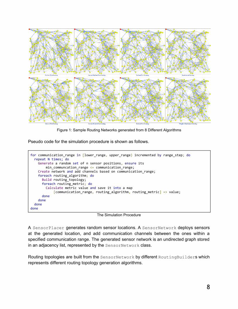
Figure 1: Sample Routing Networks generated from 8 Different Algorithms

Pseudo code for the simulation procedure is shown as follows. for communication_range in [lower_range, upper_range) incremented by range_step; do repeat N times; do Generate a random set of n sensor positions, ensure its min_communcation_range <= communication_range; Create network and add channels based on communication_range; foreach routing_algorithm; do Build routing_topology; foreach routing_metric; do Calculate metric value and save it into a map [communication_range, routing_algorithm, routing_metric] => value; done done done done

The Simulation Procedure A SensorPlacergenerates random sensor locations. A SensorNetworkdeploys sensors at the generated location, and add communication channels between the ones within a specified communication range. The generated sensor network is an undirected graph stored in an adjacency list, represented by the SensorNetwork class. Routing topologies are built from theSensorNetworkby differentRoutingBuilders which represents different routing topology generation algorithms.

8

In order to compare the routing performance, 5 routing metrics are defined to measure different characteristics of the routing topologies. While some of the metrics such as node degree variance are straightforward, some others are tricky to get right, such as Calculating Data­Aggregation and Latency metrics.

5.2.2 Routing Topology Generation Algorithms In order to route messages through the sensor network to the base station, a routing topology is needed. Routing topology generation algorithms can be categorized by single­path vs. multi­path routing, and localized vs. global routing. The tradeoffs between single­path vs. multi­path routings are, the former tends to have less energy consumption while the latter have better reliability. In real world sensor networks, it is sometimes challenging or even infeasible to apply a global / centralized routing algorithm such as the Dijkstra Algorithm, due to scalability concerns or limited access to global information. In this section we focus on single­path routing topology generation algorithms base on localized information. I.e. when choosing the routing path, each sensor only knows about nearby sensors within its communication range, and make routing decisions based on its localized knowledge. Routing topology generation is consists of 2 phases, flooding and parent selection. In the flooding phase, a discovery message is broadcasted from the base station to its neighboring sensors. The message contains the sender’s ID and routing level (the base station has level 0). A discovery message is only accepted if the receiving sensor does not yet have a routing level, or the sender has a lower level than the receiver. On accepting a discovery message, the receiver records the sender as a parent candidate for routing. By using the routing level, a sensor is guaranteed to be connected to the base station through any of its parent candidates. All routing topology generation algorithms share the same flooding phase. In the parent selection phase, different parent selection criteria are checked to select a routing parent from the parent candidates. Please note that there is no single parent selection strategy which fits all scenarios. Different strategies lead to different routing topology characteristics and accordingly different routing performance, which are evaluated by a set of routing metrics, as discussed in detail in the following section.

9

Literature [7] introduces 4 different routing topology generation algorithms: Earliest First, Nearest First, Randomized and Weighted Randomized. We implemented them all and further added 4 more algorithms, Second Earliest First, Latest First, Second Nearest First and Farthest First. Earliest First Routing is for each sensor to select the one which is the first to send discovery message to it. Similarly, Second Earliest First Routing is to select the second earliest one which sends the discovery message to the current sensor, while Latest First is to select the last one in the list. Nearest First Routing selects the candidate which has the minimum distance from the current sensor as its parent. Second Nearest First is to select the second one in the list, while Farthest First the last (which is the one with maximum distance from the current sensor). Randomized Routing, as its name indicates, is to randomly select a candidate as parent. Weighted Randomized is also random, but giving the candidates with a larger degree (i.e. with more channels connecting to neighboring sensors) less chance to be selected as parent. Intuitively the intention is to balance the energy consumption of sensors.

5.2.3 Routing Metric Calculation Algorithms To evaluate the performance of routing topology generation algorithms, a set of metrics are defined to quantify different characteristics of a routing topology. There are 5 metrics introduced in [7]. They are Node Degree Variance, Robustness, Channel Quality, Data Aggregation and Latency. While their definitions are straightforward, the actual calculations can be tricky and challenging, which will be described below. Node Degree Variance is the most straightforward metric and needs almost no further explanations. It tells whether all sensors tend to have comparable numbers of routing channels, or some of them are connected with a lot of neighbors and become hotspots, while others are relatively less connected. We can imagine that with a high node degree variance, some popular sensors will run out of energy and fail fast. Since in SensorNetwork, only the parent is stored for the routing topology, each sensor increments the children count of of its parent to get the node degree. Robustness is defined the percentage of sensors that are still connected to the base station after one most frequently used sensor (except the base station) fails. It models the reliability of the network.

10

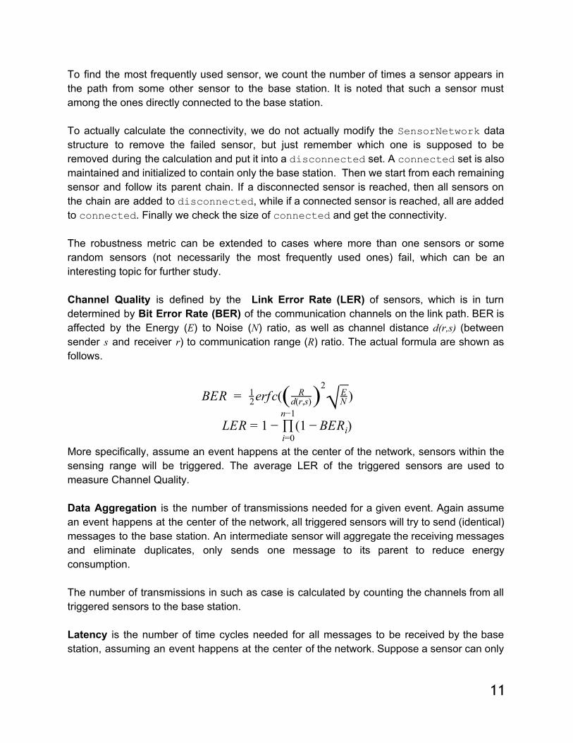
To find the most frequently used sensor, we count the number of times a sensor appears in the path from some other sensor to the base station. It is noted that such a sensor must among the ones directly connected to the base station. To actually calculate the connectivity, we do not actually modify the SensorNetworkdata structure to remove the failed sensor, but just remember which one is supposed to be removed during the calculation and put it into adisconnectedset. Aconnectedset is also maintained and initialized to contain only the base station. Then we start from each remaining sensor and follow its parent chain. If a disconnected sensor is reached, then all sensors on the chain are added todisconnected, while if a connected sensor is reached, all are added to connected. Finally we check the size of connected and get the connectivity. The robustness metric can be extended to cases where more than one sensors or some random sensors (not necessarily the most frequently used ones) fail, which can be an interesting topic for further study. Channel Quality is defined by the Link Error Rate (LER) of sensors, which is in turn determined by Bit Error Rate (BER) of the communication channels on the link path. BER is affected by the Energy (E) to Noise (N) ratio, as well as channel distance d(r,s) (between sender s and receiver r) to communication range (R) ratio. The actual formula are shown as follows.

ER erfc( ) B = 21 ( R

d(r,s))2

√EN

ER (1 )L = 1 − ∏n−1

i=0− BERi

More specifically, assume an event happens at the center of the network, sensors within the sensing range will be triggered. The average LER of the triggered sensors are used to measure Channel Quality. Data Aggregation is the number of transmissions needed for a given event. Again assume an event happens at the center of the network, all triggered sensors will try to send (identical) messages to the base station. An intermediate sensor will aggregate the receiving messages and eliminate duplicates, only sends one message to its parent to reduce energy consumption. The number of transmissions in such as case is calculated by counting the channels from all triggered sensors to the base station. Latency is the number of time cycles needed for all messages to be received by the base station, assuming an event happens at the center of the network. Suppose a sensor can only

11

receive one message at a time, so a sensor with n children sending messages will take n cycles to receive all of them, then are able to send the aggregated message to its parent. Latency is calculated by a process similar to topological sort. Starting from the triggered sensors a timestamp is assigned to their parents, which is the max of the current sensor timestamp and parent timestamp, plus one. During each iteration we start from the “leaf” sensors among the current active sensor set, then remove them from the active set before the next iteration begins. Finally timestamp of the base station is the number of total time cycles needed to transmit all messages. Routing metrics are calculated by a set of RoutingMetricCalculators, which are one of the most important and challenging part of this project.

5.2.4 Code Structures for Routing Topology Generation The routing topology generation part is written in ~2000 lines of C++ code, plus some auxiliary gnuplot scripts and Bash scripts to automatically generate and process diagrams. All code are tested under CentOS Linux (the design center workstations), and MacOSX (MacBook laptop). Tools involved are GCC (compiler), Gnuplot (version 5.0 or higher, for generating PNG diagrams. Older versions won’t generate the images correctly, but does not affect the routing topology generation and metric calculation. I installed the most recent Gnuplot on both the design center workstation and my laptop. Gnuplot 5.0 can be downloaded from http://www.gnuplot.info/download.html), ImageMagick (for combining images and convert SVG to PNG). The C++ part is composed of sensor position generation, routing topology generation, routing metric calculation, a simulation framework and a sensor network printer. The class diagram is shown as follows.

12

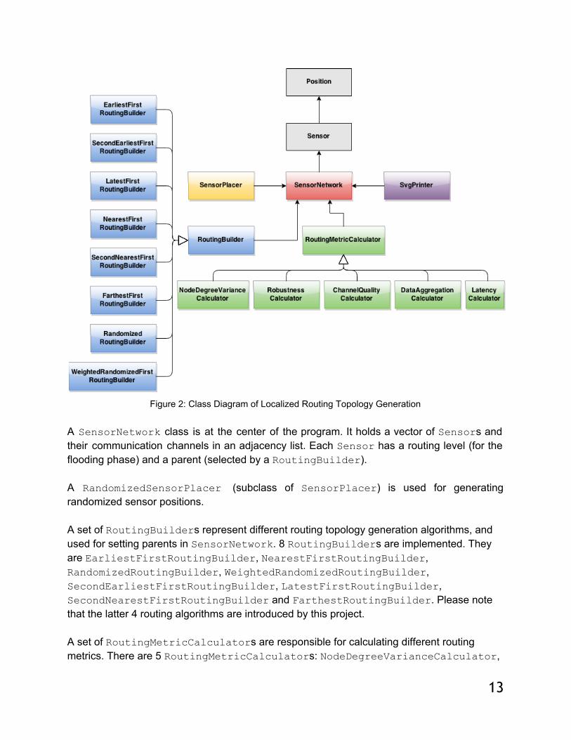
Figure 2: Class Diagram of Localized Routing Topology Generation

A SensorNetworkclass is at the center of the program. It holds a vector of Sensors and their communication channels in an adjacency list. Each Sensorhas a routing level (for the flooding phase) and a parent (selected by a RoutingBuilder). A RandomizedSensorPlacer (subclass of SensorPlacer) is used for generating randomized sensor positions. A set of RoutingBuilders represent different routing topology generation algorithms, and used for setting parents in SensorNetwork. 8 RoutingBuilders are implemented. They are EarliestFirstRoutingBuilder, NearestFirstRoutingBuilder, RandomizedRoutingBuilder, WeightedRandomizedRoutingBuilder, SecondEarliestFirstRoutingBuilder, LatestFirstRoutingBuilder, SecondNearestFirstRoutingBuilder and FarthestRoutingBuilder. Please note that the latter 4 routing algorithms are introduced by this project. A set of RoutingMetricCalculators are responsible for calculating different routing metrics. There are 5 RoutingMetricCalculators: NodeDegreeVarianceCalculator,

13

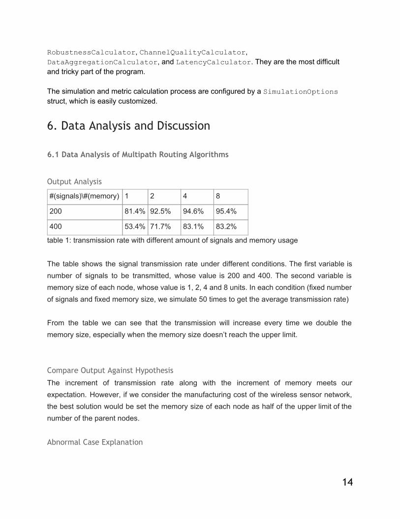
RobustnessCalculator, ChannelQualityCalculator, DataAggregationCalculator, and LatencyCalculator. They are the most difficult and tricky part of the program. The simulation and metric calculation process are configured by a SimulationOptions struct, which is easily customized.

6. Data Analysis and Discussion 6.1 Data Analysis of Multipath Routing Algorithms

Output Analysis

#(signals)\#(memory) 1 2 4 8

200 81.4% 92.5% 94.6% 95.4%

400 53.4% 71.7% 83.1% 83.2%

table 1: transmission rate with different amount of signals and memory usage The table shows the signal transmission rate under different conditions. The first variable is number of signals to be transmitted, whose value is 200 and 400. The second variable is memory size of each node, whose value is 1, 2, 4 and 8 units. In each condition (fixed number of signals and fixed memory size, we simulate 50 times to get the average transmission rate) From the table we can see that the transmission will increase every time we double the memory size, especially when the memory size doesn’t reach the upper limit. Compare Output Against Hypothesis The increment of transmission rate along with the increment of memory meets our expectation. However, if we consider the manufacturing cost of the wireless sensor network, the best solution would be set the memory size of each node as half of the upper limit of the number of the parent nodes. Abnormal Case Explanation

14

We can see that the increment of transmission rate is very little from memory size of 4 to memory size of 8. The reason is there isn’t any node in the network having more than 8 parent nodes and many of them have 4 or less parent nodes. The memory size of 4 or 8 makes no difference to them.

6.2 Data Analysis of Localized Topology Generation Algorithms The simulation is easily configurable and was performed with many different configurations. The data diagrams shown below are with 400 sensors scattered in an 100*100 square region, with communication range varying from 20.0 to 50.0 with increment step 0.1 (300 different communication ranges). With every communication range 50 sensor networks are randomly generated and average metrics values are taken to smooth the data diagram and improve confidence. For each network 8 different routing generation algorithms are applied, and for each routing topology 5 routing metrics are calculated. In total there are 15,000 different sensor networks, 120,000 different routing topologies, and 600,000 routing metrics values generated during the simulationin a single simulation configuration. In comparison, literature [7] only has 148 data points generated for 4 routing algorithms. The simulation data are output in plain text format, one file per routing metric, then fed into gnuplot scripts to generate diagrams. Diagrams for 5 routing metrics are shown and explained as follows. The first metric is Node Degree Variance. Obviously Latest First routing has the highest value, and Earliest First routing follows, which means their node degrees are very unbalanced. Farthest First, Randomized and Weighted Randomized routings are the lowest. Node degree variance increases along with the communication range, because the larger the communication range is, more choices a sensor will have for selecting parents, and sensors satisfy certain criteria are more likely to have more children.

15

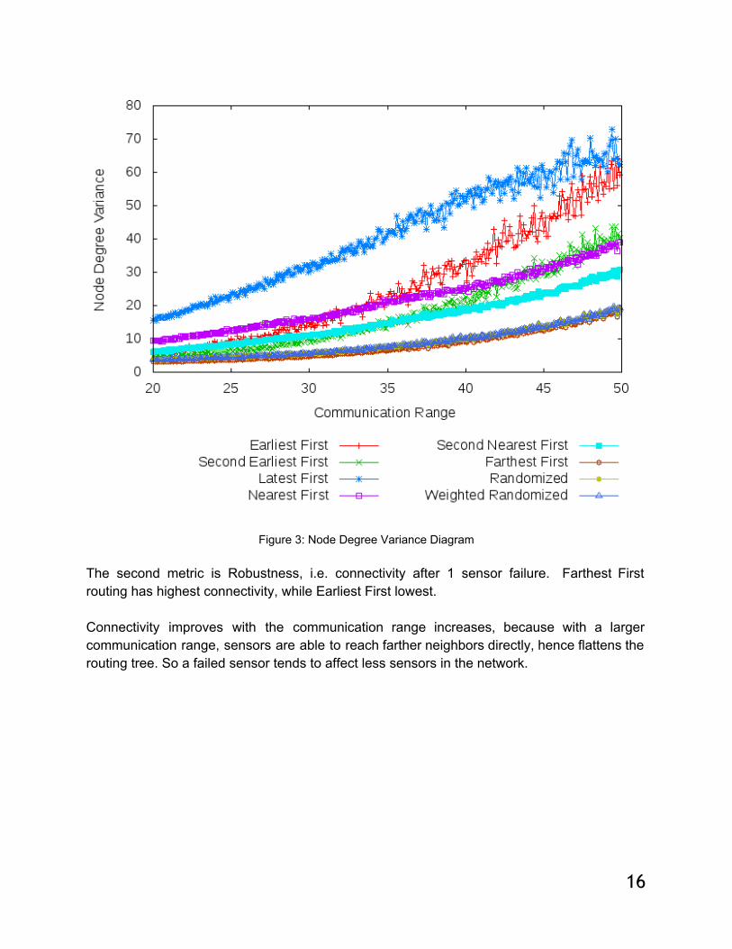
Figure 3: Node Degree Variance Diagram The second metric is Robustness, i.e. connectivity after 1 sensor failure. Farthest First routing has highest connectivity, while Earliest First lowest. Connectivity improves with the communication range increases, because with a larger communication range, sensors are able to reach farther neighbors directly, hence flattens the routing tree. So a failed sensor tends to affect less sensors in the network.

16

Figure 4: Robustness Diagram

The third metric is Channel Quality, i.e. average Link Error Rate (LER). Simulation shows Earliest First and Farthest First routings have the highest LER (worst channel quality), while Nearest First routing the lowest LER (best channel quality). It is easily understood because longer channels have higher Bit Error Rate (BER). LER improves with communication range increase, because with higher communication range, the channel distance to communication range ratio drops, and channel BER improves.

17

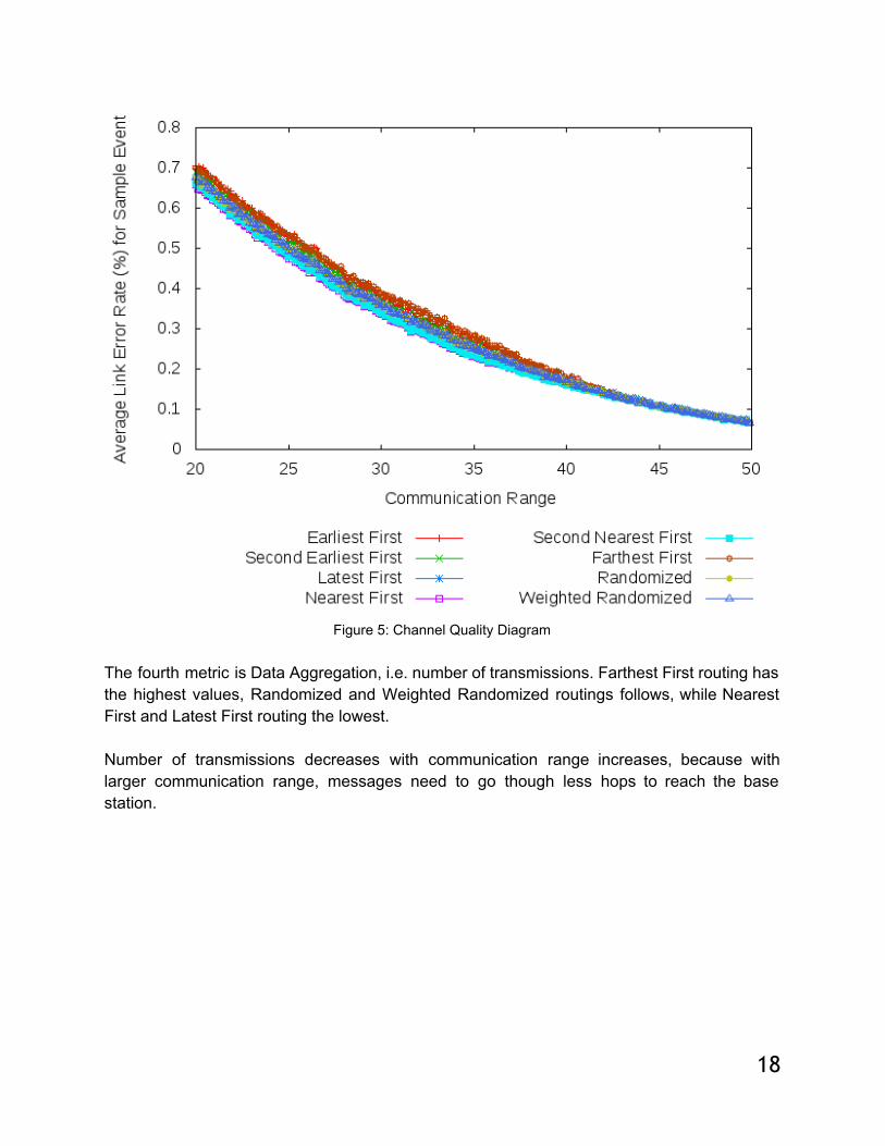
Figure 5: Channel Quality Diagram

The fourth metric is Data Aggregation, i.e. number of transmissions. Farthest First routing has the highest values, Randomized and Weighted Randomized routings follows, while Nearest First and Latest First routing the lowest. Number of transmissions decreases with communication range increases, because with larger communication range, messages need to go though less hops to reach the base station.

18

Figure 6: Data Aggregation Diagram The last metric is Latency, i.e. number of time cycles. This diagram is the noisiest. With a lower communication range, Latest First routing is the worst, Nearest First follows; At a higher communication range, Farthest First becomes the worst while Second Nearest First the best. As the increase of communication range, latency fluctuates a lot. At very high communication range, latency increases because more sensors are directly connected to fewer (and farther) parents, and parallel transmissions becomes less applicable (because a sensor can only receive one message from one of its children at a time).

19

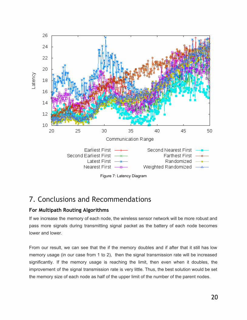
Figure 7: Latency Diagram

7. Conclusions and Recommendations For Multipath Routing Algorithms

If we increase the memory of each node, the wireless sensor network will be more robust and pass more signals during transmitting signal packet as the battery of each node becomes lower and lower. From our result, we can see that the if the memory doubles and if after that it still has low memory usage (in our case from 1 to 2), then the signal transmission rate will be increased significantly. If the memory usage is reaching the limit, then even when it doubles, the improvement of the signal transmission rate is very little. Thus, the best solution would be set the memory size of each node as half of the upper limit of the number of the parent nodes.

20

For Localized Topology Generation Algorithms

We also implemented 8 localized single­path routing topology generation algorithms (4 of them are introduced in this project), implemented 5 routing metric calculation algorithms for routing networks, performed comprehensive large scale simulations with different settings, generated metric diagrams comparing performance of the 8 routing algorithms and analyzed the data. It turns out that there is no single best routing generation algorithm which fits all different scenarios. Each generation algorithm has its own advantage and disadvantage. We should choose the right algorithm according to our actual demand. For example, if we want our network to have strong connection and could tolerate spending more time for transmission, then Farthest First routing would be a good choice since it has highest connectivity but needs more time at a higher communication range. Recommendations for the future studies

In the future studies, for multipath routing, we are going to optimize the algorithm, especially the DFS algorithm, so that we can simulate with more nodes in the area and larger memory. In the DFS algorithm we implemented in multipath routing, we have to find all the available paths, and then choose the first one as the shortest path, which holds lots of the resources of CPU and memory of our laptops. If we can find an algorithm that is able to find the shortest path without looking for all other paths, the multipath routing algorithm would be more efficient. Further studies for the localized routing topology generation may develop smarter algorithms for parent selection, and define more metrics to better predict the network performance.

Bibliography [1] Al­Karaki, Jamal N., and Ahmed E. Kamal. "Routing techniques in wireless sensor networks: a survey." Wireless communications, IEEE 11.6 (2004): 6­28. [2] Jung, Eunjae, and Duncan M. Hank Walker. "Reliable energy efficient routing in wireless sensor networks." MASS. 2005. [3] Karaboga, Dervis, Selcuk Okdem, and Celal Ozturk. "Cluster based wireless sensor network routing using artificial bee colony algorithm." Wireless Networks 18.7 (2012): 847­860.

21

[4] Singh, Dhirendra Pratap, Yash Agrawal, and Surender Kumar Soni. "Energy optimization in Zigbee using prediction based shortest path routing algorithm." Emerging Trends and Applications in Computer Science (NCETACS), 2012 3rd National Conference on. IEEE, 2012. [5] Akkaya, Kemal, and Mohamed Younis. "A survey on routing protocols for wireless sensor networks." Ad hoc networks 3.3 (2005): 325­349. [6] Pavithra, B. S., and A. Asha. "An optimized routing approach in wireless sensor networks." Information Communication and Embedded Systems (ICICES), 2014 International Conference on. IEEE, 2014. [7] Zhou, Congzhou, and Bhaskar Krishnamachari. "Localized topology generation mechanisms for wireless sensor networks." Global Telecommunications Conference, 2003. GLOBECOM'03. IEEE. Vol. 3. IEEE, 2003. [8] B. Krishnamachari, D. Estrin, and S. Wicker, “The Impact of Data Aggregation in Wireless Sensor Networks,” In International Workshop on Distributed Event­Based Systems, Vienna, Austria, July 2002. [9] S. Ni, Y. Tseng, Y. Chen, and J. Sheu, “The Broadcast Storm Problem in a Mobile Ad Hoc Network,” In ACM MOBICOM’99, August 1999. [10] D. Ganesan, B. Krishnamachari, A. Woo, D. Culler, D. Estrin, and S. Wicker, “Large­scale Network Discovery: Design Tradeoffs in Wireless Sensor Systems,” Poster presented at the 18th ACM Symposium on Operating System Principles, Banff, Canada, October 2001.

22