AD-AO6S 123 ROYAL AIRCRAFT ESTABLISHMENT FARNBOROUGH (ENGLANDI F/6 1/2THE FORM4 OF T. SOLTIONS OF THE LINEAR INTEGRO-DIFFERENTIAL FB--ETC(UISEP 79 D L WOODCOCK

UNCLASSIFIED RAE-TM STRUCTS56DRIC R70935 ML

L136

11fl2.0

11111L2 111.

MICROCOPY RESOLUTION TEST CHART

STRUCTURES 956 STRUCTURES 956

ROYL IRLEVrV L~ISHMENTROALAICRAFT E B

FE

& THE FORM OF THE SOLUTIONS OF THE LINEAR INTEGRO-DIFFEBENTIAL

I EQUATIONS OF SUBSONIC AEROELASTICITY

by

D. L. Woodcock

September 1979

Lk

LA.

80 1 28 .0

ROYAL A I RC RAFT A,-rqT A-PT' L SHME NT

IQ i ja r[tTechnical emoSrS es-956

Received for printing 25 Septembei 1979

4 THE FORM OF THE,,SOLUTIONS OF THE -IFERETIA

- ~ ~ ~~INEAR,TEGRO,-IFRETA

SEQUATIONS OF PUBSONIC AEROELASTICITY

by

SUHMARY

The solution of the subsonic flutter problem, when the commonly used

linear differential equation model is replaced by the more correct linear integro-

differential equation model, is studied and the nature of the system's free

motion established. The different forms appropriate to two-dimensional and three-

dimensional flow, and to the cases when the system has a zero characteristic

value, are developed in detail. It is shown that, for large time t , the

behaviour can variously be like t or t

Controller JMSO London

1979

AI

2

LIST OF CONTENTS

Page

I INTRODUCTION 3

2 EQUATIONS OF MOTION 3

3 APPROXIMATIONS TO THE EQUATION OF MOTION 7

4 THE NATURE OF THE SOLUTION 9

4.1 General 9

4.2 Particular cases 14

4.3 Discussion 18

5 CONCLUDING REMARKS 18

Appendix A Laplace transforms of logmt and inverse Laplace transforms

of logmp 21

Appendix B The right hand Dirac delta function and its use in Laplace

transform theory 33

Tables 1-3 39

List of symbols 42

References 46

Report documentation page inside back cover

AG ion For

DZC TABUnun c sd

: iction

• 1 a .Ar,1

\Dlst special

" |

'*

1BR70935

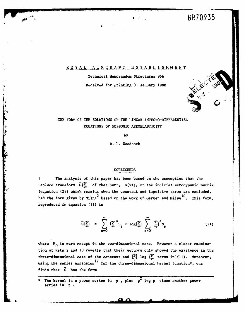
ROYAL AIRCRAFT ESTABLISHMENT

Technical Memorandum Structures 956

Received for printing 31 January 1980 '

THE FORM OF THE SOLUTIONS OF THE LINEAR INTEGRO-DIFFERENTIAL

EQUATIONS OF SUBSONIC AEROELASTICITY

by

D. L. Woodcock

CORRIGENDA

I The analysis of this paper has been based on the assumption that the

Laplace transform G of that part, G(vT), of the indicial aerodynamic matrix

(equation (2)) which remains when the constant and impulsive terms are excluded,2 10had the form given by Milne based on the work of Garner and Milne 0 . This form,

reproduced in equation (11) is

e )L + iog819 (11)Ss=O smfO

where NO0 is zero except in the two-dimensional case. However a closer examina-

tion of Refs 2 and 10 reveals that their authors only showed the existence in the

three-dimensional case of the constant and (') log (I) terms in" (I). Moreover,• 17 .

using the series expansion for the three-dimensional kernel function*, one

finds that G has the form

The kernel is a poer series in p , plus p2 log p times another powerseries in p

-A

2

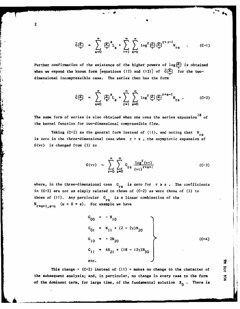
= Ls + logr() -v" ;-IN (C-I)vv iLvv rs

s=O r-1 s=r

Further confirmation of the existence of the higher powers of log( ) is obtained

when we expand the known form (equations (12) and (13)) of a( ) for the two-

dimensional incompressible case. The series then has the form

00 00 r r+s-1

= + log N (C-2)s .Z"Z rs

s=0 r=1 s-O

The same form of series is also obtained when one uses the series expansion 18 of

the kernel function for two-dimensional compressible flow.

Taking (C-2) as the general form instead of (11), and noting that Nrs

is zero in the three-dimensional case when r > s , the asymptotic expansion of

G(vT) is changed from (3) to

G(VT) Z Z Grs G log r)r( (C-3)

r-0 s-0r.(T sl

where, in the three-dimensional case G is zero for r i s The coefficientsrs

in (C-3) are not as simply related to those of (C-2) as were those of (3) to

those of (11). Any particular G is a linear combination of the

Nr+u+is.u (u 0 + s). For example we have

G00= -N 10

G = N + (2 - 2)N 2001 11 2

Gi0 0 - 2N2 0 (C-4)

G 4N21 + (18 - 12y)N30

etc.

This change - (C-2) instead of (11) - makes no change to the character of

the subsequent analysis; and, in particular, no change in every case to the form

of the dominant term, for large time, of the fundamental solution X . There is

3

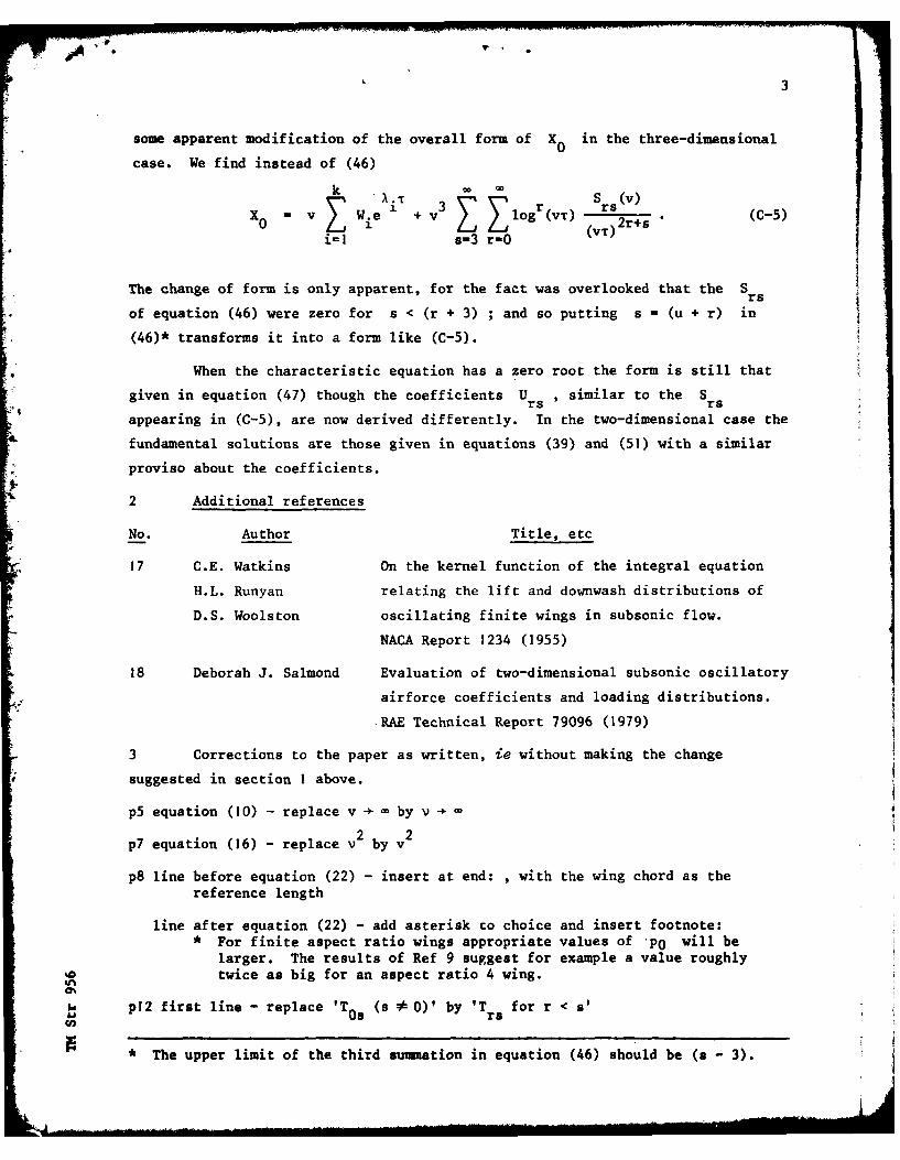
some apparent modification of the overall form of X0 in the three-dimensional

case. We find instead of (46)

A. 3iN S rs(v)

X0 - v Wie 1 + v (VT (VT)2r+s (C-5)

iffi s=3 r-O

The change of form is only apparent, for the fact was overlooked that the Srs

of equation (46) were zero for s < (r + 3) ; and so putting s = (u + r) in

(46)* transforms it into a form like (C-5).

When the characteristic equation has a zero root the form is still that

given in equation (47) though the coefficients U , similar to the Srs rs

appearing in (C-5), are now derived differently. In the two-dimensional case the

fundamental solutions are those given in equations (39) and (51) with a similar

proviso about the coefficients.

2 Additional references

No. Author Title, etc

17 C.E. Watkins On the kernel function of the integral equation

H.L. Runyan relating the lift and downwash distributions of

D.S. Woolston oscillating finite wings in subsonic flow.

NACA Report 1234 (1955)

18 Deborah J. Salmond Evaluation of two-dimensional subsonic oscillatory

airforce coefficients and loading distributions.

RAE Technical Report 79096 (1979)

3 Corrections to the paper as written, ie without making the change

suggested in section I above.

p5 equation (10) - replace v by v2 2

p7 equation (16) - replace v by v

p8 line before equation (22) - insert at end: , with the wing chord as thereference length

line after equation (22) - add asterisk to choice and insert footnote:

* For finite aspect ratio wings appropriate values of PO will be

larger. The results of Ref 9 suggest for example a value roughlytwice as big for an aspect ratio 4 wing.

pI2 first line - replace 'To (s * 0)' by 'Ts for r < s'

* The upper limit of the third summation in equation (46) should be (s - 3).

4

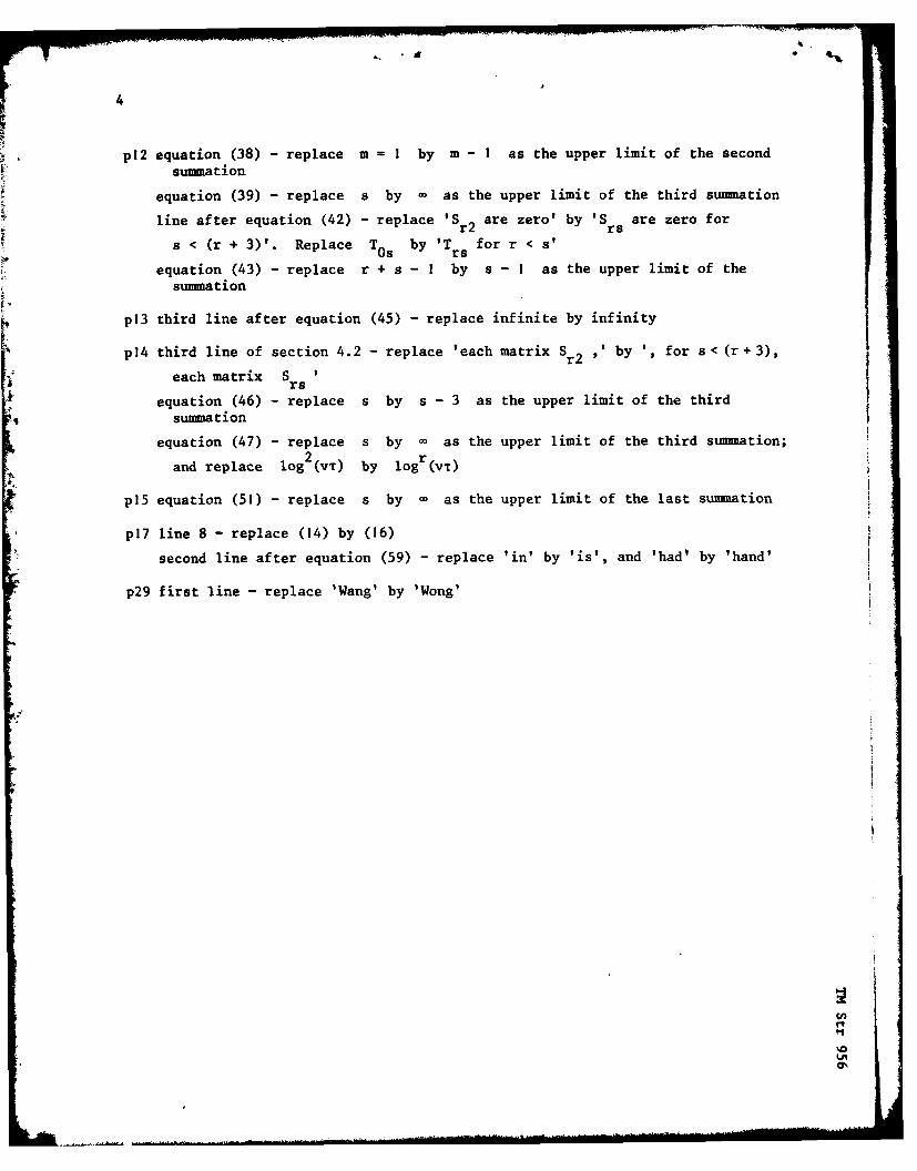
p12 equation (38) - replace m = I by m - I as the upper limit of the second

summation

equation (39) - replace s by - as the upper limit of the third summation

line after equation (42) - replace 'St2 are zero' by 'S are zero forr2 rs

s < (r + 3)'. Replace TOs by 'Trs for r < s'

equation (43) - replace r + s - I by s - I as the upper limit of the

summation

p13 third line after equation (45) - replace infinite by infinity

p14 third line of section 4.2 - replace 'each matrix Sr2 ,' by ', for s< (r+3),

each matrix S rrs

equation (46) - replace s by s - 3 as the upper limit of the thirdsummation

equation (47) - replace s by - as the upper limit of the third summation;

and replace log 2(vT) by logr (vT)

p15 equation (51) - replace s by - as the upper limit of the last summation

p17 line 8 - replace (14) by (16)

second line after equation (59) - replace 'in' by 'is', and 'had) by 'hand'

p29 first line - replace 'Wang' by 'Wong'

5

DISTRIBUTION:

D/SARI (DOI), Monsanto HouseNPO, Teddington, MiddxSecretary, Aeronautical Research Council,National Physical Laboratory,Teddington, Middx

DRIC

BAe Weybridge - Mr B.W. PayneBAe Warton Mr C.G. LodgeBAe Manchester Mr M.J. GreenBAe Kingston Mr C.W. SullivanBAe Hatfield Mr A.G. WoodsWestland Helicopter Ltd Mr D.E. BalmfordCAA, Redhill Mr D.O.N. James

Dr T. Ichikawa,NAL, Aeroelasticity Section,1880 Jindaiji, Machi, Chofu, Tokyo, Japan

Dr V.J.E. Stark,Saab-Scania, Aerospace Div 5-581,88 Linkopinc, Sweden

Dr W.P. Rodden,255 Starlight Crest Drive, La Canada,California, 91011, USA

H.J. Hassig,Flight Dynamics Dept., Lockheed,2555 North Hollywood Way, Burbank,California, 91503, USA

R.C. Schwanz,Wright-Patterson Air Force Base,Dayton, Ohio, 45433, USA

Prof. H. Ashley,Dept. of Aeronautics & Astronautics,Stamford University, Stamford,California, 94305, USA

Prof. B. Etkin,University of Toronto,Institute of Aerospace Studies,Toronto 5, Ontario

Dr S. Parthan,Hindustan Aeronautics Ltd.,Bangalore, 560017, India

RAE

LibraryBedford LibraryHead of Structures DepartmentHead of Aerodynamics DepartmentHead of Mathematics and Computation DepartmentHead of ST4 Division

0%il i l . . . .. . i! . . .. I l i .. l ... .

.~ -

4

I

3

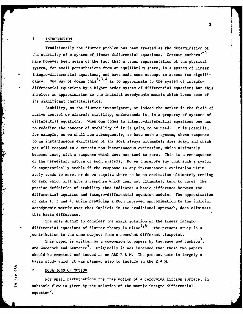
I INTRODUCTION

Traditionally the flutter problem has been treated as the determination of

the stability of a system of linear differential equations. Certain authors1- 4

have however been aware of the fact that a truer representation of the physical

system, for small perturbations from an equilibrium state, is a system of linear

integro-differential equations, and have made some attempt to assess its signifi-

cance. One way of doing this 1,3 ,4 is to approximate to the system of integro-

differential equations by a higher order system of differential equations but this

involves an approximation to the indicial aerodynamic matrix which loses some of

its significant characteristics.

Stability, as the flutter investigator, or indeed the worker in the field of

active control or aircraft stability, understands it, is a property of systems of

differential equations. When one comes to integro-differential equations one has

to redefine the concept of stability if it is going to be used. It is possible,

for example, as we shall see subsequently, to have such a system, whose response

to an instantaneous excitation of any sort always ultimately dies away, and which

yet will respond to a certain non-instantaneous excitation, which ultimately

becomes zero, with a response which does not tend to zero. This is a consequence

of the hereditary nature of such systems. Do we therefore say that such a system

is asymptotically stable if the response to any instantaneous excitation ultim-

ately tends to zero, or do we require there to be no excitation ultimately tending

to zero which will give a response which does not ultimately tend to zero? The

precise definition of stability thus indicates a basic difference between the

differential equation and integro-differential equation models. The approximation

of Refs 1, 3 and 4, while providing a much improved approximation to the indicial

aerodynamic matrix over that implicit in the traditional approach, does eliminate

this basic difference.

The only author to consider the exact solution of the linear integro-2,6

differential equations of flutter theory is Milne '6 . The present study is a

,contribution to the same subject from a somewhat different viewpoint.

This paper is written as a companion to papers by Lawrence and Jackson3

4and Woodcock and Lawrence . Originally it was intended that these two papers

should be combined and issued as an ARC R & M. The present note is largely a

basic study which it was planned also to include in the R & M.

2 EQUATIONS OF MOTION

For small perturbations the free motion of a deforming lifting surface, in

subsonic flow is given by the solution of the matrix integro-differential

equationS"

4

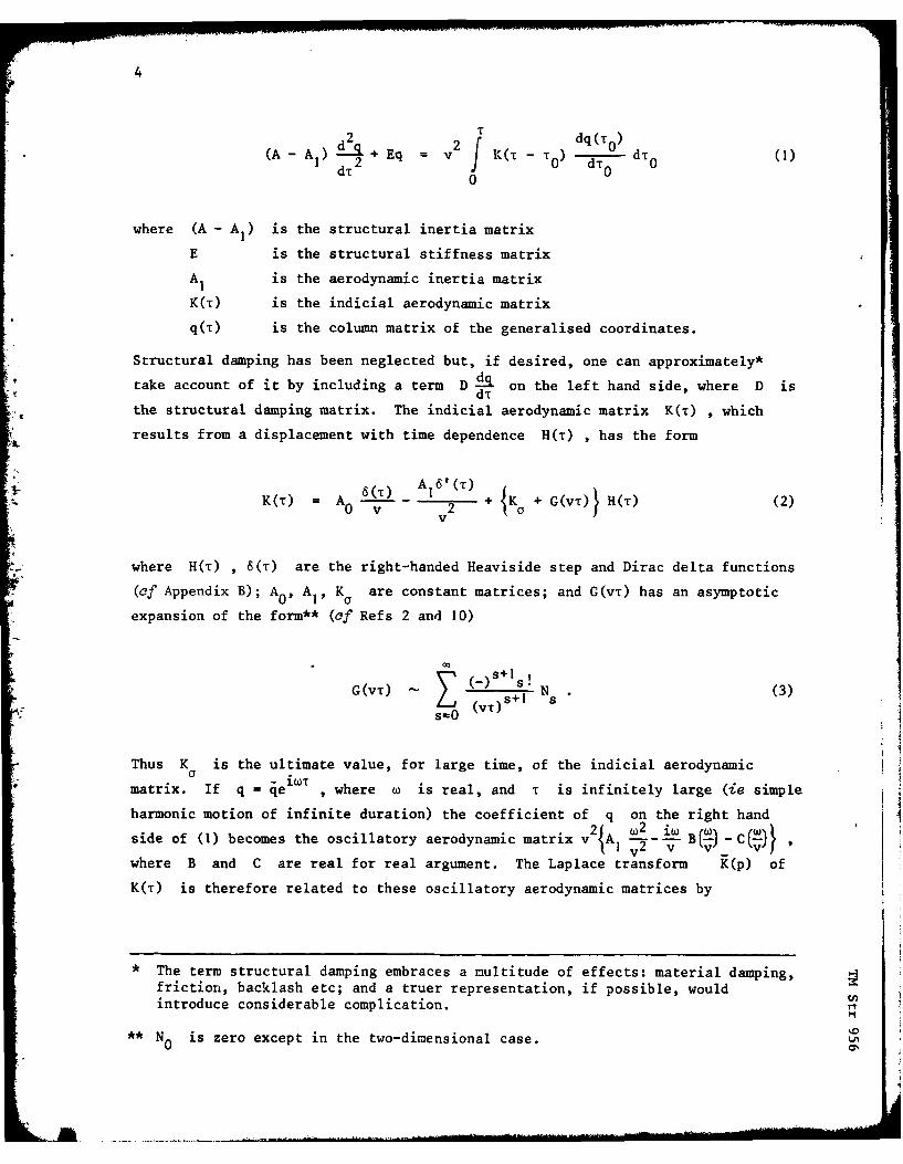
2 2 T dq (T0)(A - A1 d + Eq = v2 K(T - 0 ) dt (1)0

where (A - A1) is the structural inertia matrix

E is the structural stiffness matrix

A is the aerodynamic inertia matrix

K(r) is the indicial aerodynamic matrix

q(T) is the column matrix of the generalised coordinates.

Structural damping has been neglected but, if desired, one can approximately*

take account of it by including a term D & on the left hand side, where D isdtu

the structural damping matrix. The indicial aerodynamic matrix K(T) , whichresults from a displacement with time dependence H(T) , has the form

K(T) = A0 6(T) A6'(r) + (v 2 + K + G(VT) H(T) (2)

where H(T) , 6(T) are the right-handed Heaviside step and Dirac delta functions

(cf Appendix B); A0, Al, Ka are constant matrices; and G(vr) has an asymptotic

expansion of the form** (of Refs 2 and 10)

G(vT) -)+ s! N (3):' s O (v-[)S~

Thus K is the ultimate value, for large time, of the indicial aerodynamic

matrix. If q = qe , where w is real, and T is infinitely large (ie simple

harmonic motion of infinite duration) the coefficient of q on the right hand

side of (1) becomes the oscillatory aerodynamic matrix v2 A! B -,W)where B and C are real for real argument. The Laplace transform K(p) of

K(T) is therefore related to these oscillatory aerodynamic matrices by

* The term structural damping embraces a multitude of effects: material damping,friction, backlash etc; and a truer representation, if possible, wouldintroduce considerable complication.

** N0 is zero except in the two-dimensional case.

0I

5

pK (p) $ A + P- B( ) + C( 2) (4)

where B and C are now continued analytically into the complex plane.

Relationships therefore exist between the matrices appearing in (2) and the

oscillatory aerodynamic matrices. Using the theorem | that

Vt PY = Y( ) (5)

where y is any function* and y its Laplace transform, we immediately see

that

K = -C(O) (say)- C . (6)

Now, from (2)

pK(p) = K + R A0 + 2- )2A, (7)CY v0 v, v

and so (4) can be rewritten

P- A +(2) C= c- C(P RB( (8)v Iv v I

If now we go to the limit p = ioo we get the relationships

A0+ 1G(ioc)I f - B(-) = (say) - B, (9)

VtLv-0a(iv)!] = CO - C(-) - (say) CO - C, .(0

From the work of Milne2 we know that Gv ) taken as single valued in theV

complex plane cut along the negative real axis, has the form (of equation (3) and

Appendix A)

(.2) s + log.. (2)SN (1

s=O s=O

* Strictly any function which is bounded for real T > 0. We apply the theorem

to the last term of (2).

?A

6

where N is zero except in the two-dimensional case. In the particular case of

two-dimensional incompressible flow it is easily seen, from the known analytical

solution (eg Ref 12) that G) has the form(VE

(S ( PT (12)

where R, S, T are constant matrices and ( is the Theodorsen function

1 K(_2_V) (13)

which is taken as single valued in the complex plane apart from a slit along the

negative real axis.

When the results of Appendix A (in particular equation (A-55)) are applied,

in conjunction with (B-I), to equation (11) one obtains an expression for G(vT)

which is the asymptotic expansion given in equation (3) plus an infinite number

of terms involving the 6 function and its derivatives. Thus we obtain

G(VT) SH(T) + -6(T) + -6'(T) +s+1 2(VT C) ss=0 (v)S

(N N- (y + log VT)- 6 (T) + 6'(T) +

vCI2Ni= 6 ( T) + ... . ...

..... (14)

As pointed out in Appendix B such series as those enclosed in the in

(14) represent functions which are transcendentally small compared with the

negative power of T . The same is clearly true of log T or T x such a

series. Thus the term in the square brackets in (14), which we will call

G(vT) , satisfies the conditiont0(

i. nG(v)I = 0 (n O (15) a'

7

and so has a zero asymptotic expansion in terms of the gauge functions (vT)

Any function satisfying (15) can be interpreted (of Appendix B) as the sum of a

function which is zero for T greater than some finite value, a number of a

decaying exponential expl- aTb, (a > 0, b > 0), and possibly a finite number of

6 functions*. There is, however, no reason why G(vT) should have non-smooth

behaviour at any positive T .

One further point to note is that the aerodynamic (or virtual) inertia

matrix A , is zero if the flow is compressible. Finally we write the equation

of motion (I) in the following alternative form, using (2),

T2 A v dq(T 0 )

~~ 2 ___ 0 T(6A 1 - + (E - Kov 2 )q = v G(v - VT 0 ) d0 (16)00 0

3 APPROXIMATIONS TO THE EQUATION OF MOTION

The most common approximation is to assume that the function G , in the

expression for the indicial aerodynamic matrix (equation (2)), is zero and that

the constant matrices A0 , K have the values -B(v), - C(v) respectively

where v is an assumed value of the frequency parameter. Thus instead of

equations (6) and (9) the approximations

K = - C(v) (17)

0r

A0 M - B(v) (18)

-t o (19)V.

0

are made. The purpose of this approximation is to obtain a differential equation

which has a solution which is identical, for large time, with a solution of the

original equation ((I) or (16)) in the particular case when the latter solution

ultimately becomes sinusoidal with frequency parameter v . This differential

equation has the form

A A!2 + vB(v) d + (v2C(v) + E)q - 0 . (20)dr

~ * This expression, hereinafter, refers to a selection from 6(T) and all the

6(n) (T)

-MEMO

8

A rather better approximation, due to Richardson is to approximate to G

in equation (2) by a finite power series multiplied by a decaying exponential

term

G(vT) e 01 1Kr-0 rZ(21)

r=0

Here m is a positive integer and p0 a positive scalar. In the two-

dimensional incompressible case, for the modes of heave and pitch, an established

good approximation to G (see Lomax 9) has the temporal behaviour

0*9-o -0.6vT(e-0 9vt + 2e- ) . (22)

This suggests that a suitable choice for p0 in the approximation (21) lies in

the range 0.09 - 0.6. With this approximation (equation (21))

m- Kr (POV)rv(P r 0- p0- +1 (23)

rV0 (p + p~v)

It will be noticed, comparing equation (3) or (14) with (21), or (11) with (23),

that this approximation to G (and hence to the indicial aerodynamic matrix)

does not have the right behaviour as T tends to oo ; nor, of course, does its

transform have the right behaviour as p tends to nought, or - p0v . A suitable

procedure for the determination of the K coefficients is described in Ref 3.r

In particular from equations (9), (10) and (23)

A 0 = - B (24)

K0 = C0 - C . (25)

In the applications of this approximation, in Refs 3 and 4, the relationship (25)

was not used, it being preferred to give equal weight to the values of the

oscillatory aerodynamic matrices, at a set of frequency parameters, in the

determination of the K coefficients.r C

'1

Ln

soft"

9

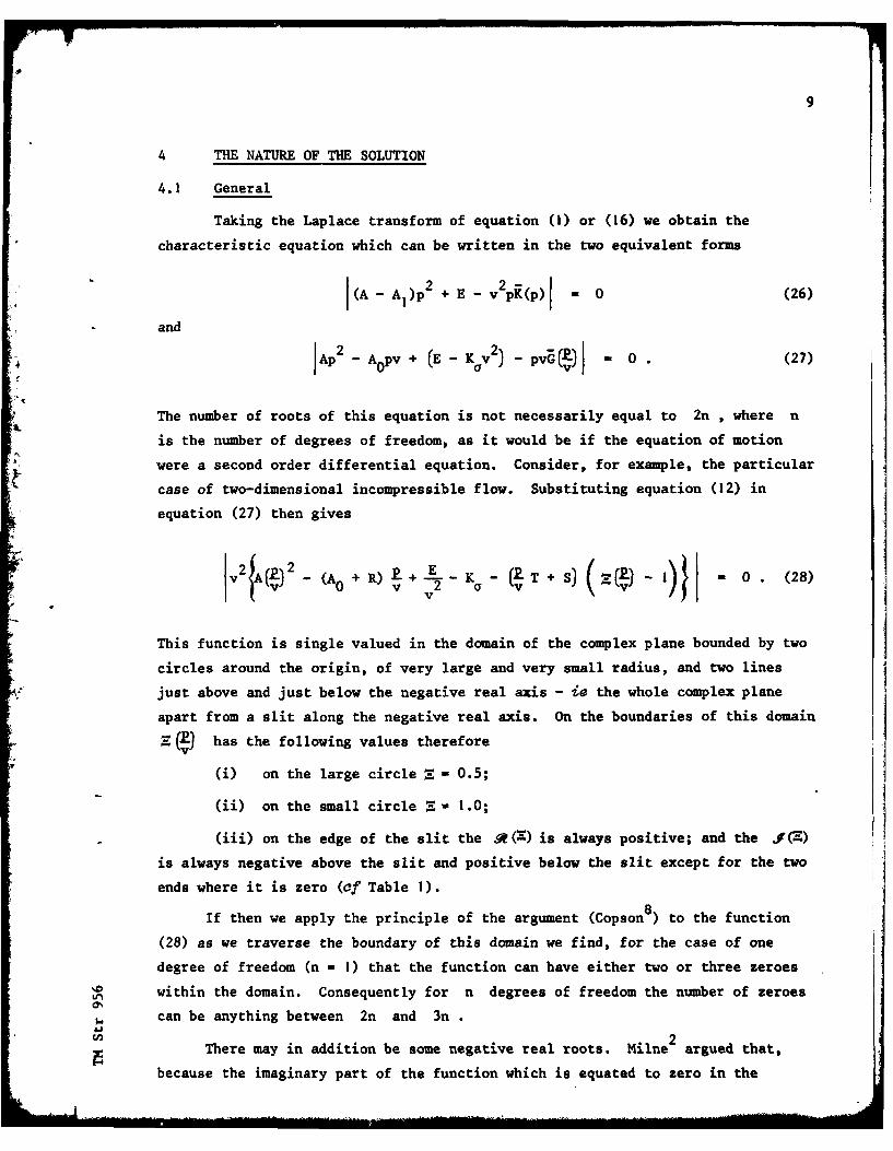
4 THE NATURE OF THE SOLUTION

4.1 General

Taking the Laplace transform of equation (1) or (16) we obtain the

characteristic equation which can be written in the two equivalent forms

I(A- A)p 2 + E - v2pK(p)j - 0 (26)

and

jAp2 A~pv + (E - K av) -v Pv(J 0 .(27)

The number of roots of this equation is not necessarily equal to 2n , where n

is the number of degrees of freedom, as it would be if the equation of motion

were a second order differential equation. Consider, for example, the particular

case of two-dimensional incompressible flow. Substituting equation (12) in

equation (27) then gives

v2JA ()2 A + R) k + Kc0 T- S 0 .(28)

V v 2v

This function is single valued in the domain of the complex plane bounded by two

circles around the origin, of very large and very small radius, and two lines

just above and just below the negative real axis - ie the whole complex plane

apart from a slit along the negative real axis. On the boundaries of this domain

V(.) has the following values therefore

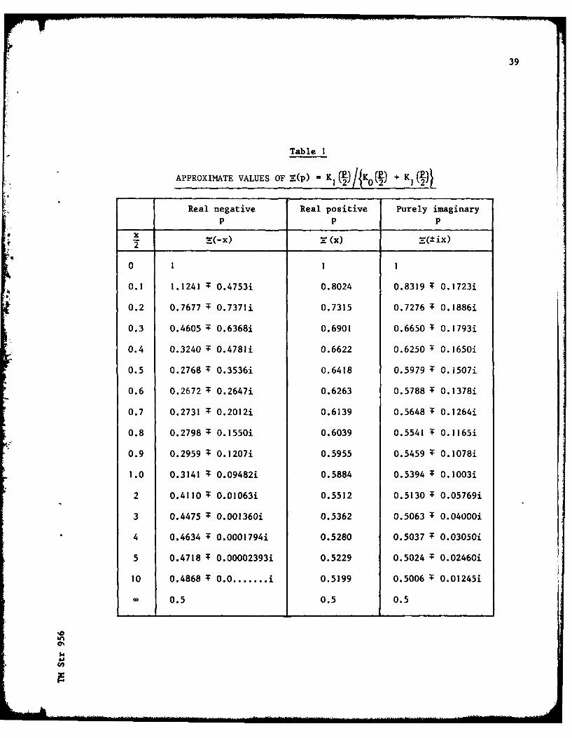
() on the large circle - 0.5;

(ii) on the small circle Z - 1.0;

(iii) on the edge of the slit the R(A) is always positive; and the J()

is always negative above the slit and positive below the slit except for the two

ends where it is zero (of Table 1).

If then we apply the principle of the argument (Copson8) to the function

(28) as we traverse the boundary of this domain we find, for the case of one

degree of freedom (n - 1) that the function can have either two or three zeroes

n within the domain. Consequently for n degrees of freedom the number of zeroes

d can be anything between 2n and 3n

There may in addition be some negative real roots. Milne2 argued that,

because the imaginary part of the function which is equated to zero in the

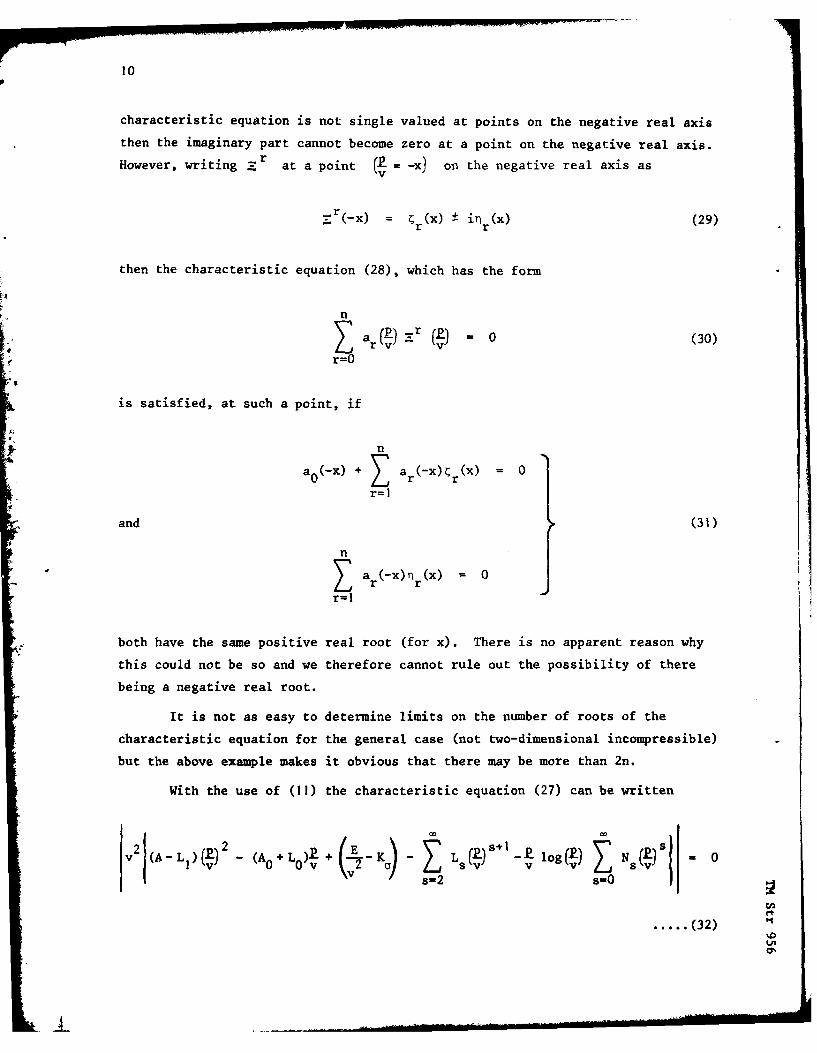
10

characteristic equation is not single valued at points on the negative real axis

then the imaginary part cannot become zero at a point on the negative real axis.

However, writing Zr r at a point (R = -x) on the negative real axis asvl

r(x)= r x : i (x) (29)

then the characteristic equation (28), which has the form

nZ a(J: (J 0 (30)

r=0

is satisfied, at such a point, if

n

a 0(x)+Z ar(-X)r = 0

r=1

and (31)

n

Z ar(-X)nr(x) = 0

r=I

both have the same positive real root (for x). There is no apparent reason why

this could not be so and we therefore cannot rule out the possibility of there

being a negative real root.

It is not as easy to determine limits on the number of roots of the

characteristic equation for the general case (not two-dimensional incompressible)

but the above example makes it obvious that there may be more than 2n.

With the use of (11) the characteristic equation (27) can be written

(A-LI) - (A0 +L0 )k + -K - Z Ls ) '- k log() E Ns = 0

...... (32)

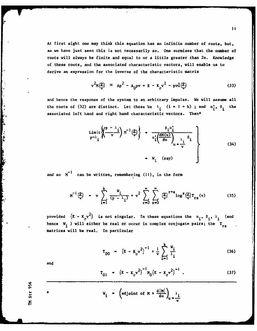
• II

At first sight one may think this equation has an infinite number of roots, but,

as we have just seen this is not necessarily so. One surmises that the number of

roots will always be finite and equal to or a little greater than 2n. Knowledge

of these roots, and the associated characteristic vectors, will enable us to

derive an expression for the inverse of the characteristic matrix

v2(P - Ap2 - Aopv + E - K v 2 - pvGa (33)

and hence the response of the system to an arbitrary impulse. We will assume all

the roots of (32) are distinct. Let these be A. (i - I - k) ; and a!, 8. the

associated left hand and right hand characteristic vectors. Then*

Limit I) va dM = 1u)

i iun- -(34)

v

= W. (say)i

-Iand so M can be written, remembering (II), in the form

M I V 2 Z Z rv2Z logS£) T (v) (35)-- "V -v" rsi- r-O s=O

provided (E - Kcv 2) is not singular. In these equations the ai, si, Xi (and

hence W. ) will either be real or occur in complex conjugate pairs; the T1 rs

matrices will be real. In particular

kTOO E Kv2-1 1 Z Wi

T - - + - (36)i-I! (6

and

To, - (E - Kav 2 NO(E - Kav2) (37)

0%

1i (adjoint of M x du I~v

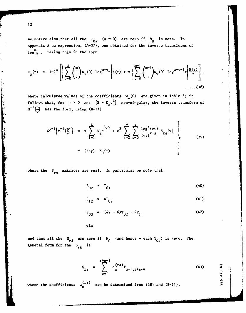
12

We notice also that all the TOs (s * 0) are zero if N is zero. In

Appendix A an expression, (A-37), was obtained for the inverse transforms ofm

log p . Taking this in the form

Sn-v-II H()]

() ()m ) W (0) log-v T6(T) + m (0) log Tm = vT

..... (38)

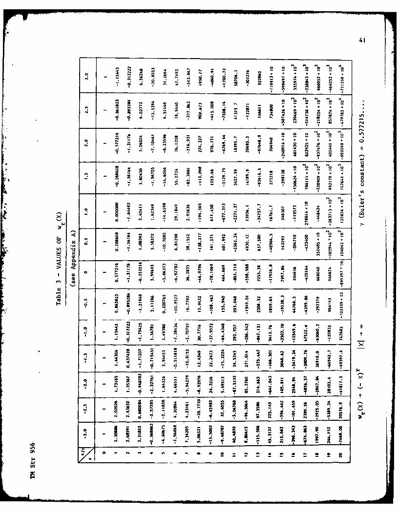
where calculated values of the coefficients w (0) are given in Table 3; itV

follows that, for T > 0 and (E - K v2) non-singular, the inverse transform of

M- ) has the form, using (B-I)

V 1k 00i r

1.- 3 lgr(vT)- - ffiv W.e v S (v)v (VT )r+s r

i=l s=2 r=0 (39)

= (say) X0 (t)

where the S matrices are real. In particular we note thatrs

S0 2 = T01 (40)

S1 2 = 4T0 2 (41)

S03 (4y - 6)T0 2 - 2Tll (42)

etc

and that all the Sr2 are zero if N (and hence - each T0s) is zero. The

general form for the Srs is

r+s-l

S a Z rS)T (43)Srs Zj u u-|, r+s-u

S(ra)where the coefficients a can be determined from (38) and (B-II).

u

13

It will be noticed that an infinite series of terms in the 6 function

and its derivatives has apparently been omitted from (39). The coefficients in

this series, which by (B-Il) are constants, cannot easily be evaluated since they

are the limit (T - 0) of rather complicated sums of terms each of which

individually becomes infinite at the limit. We assume that each coefficient has

an appropriate finite value*. Then, as shown in Appendix B, the series omitted

from (39) represents a function which is either zero for T greater than some* -ar

finite value, or else decays, as T - , as a simple exponential e or more

rapidly. There is no reason why X0 should have any non-smooth behaviour at

finite T , and we have already included in (39) all the possible simple

exponential terms. Consequently the function omitted, if it is not a null

function, must be a function which decays more rapidly, with increasing T

than any of the terms we have given in the above expression for X0

(equation (39)).

An arbitrary instantaneous excitation at T = 0+ can be taken to be

6(T)f 0 + 6 (1)(T)f I + 6(2) (T)f 2 +

where fop fl I "." are arbitrary real constant column matrices; and so the

free motion of the system (ie the motion after the disturbance) is given by

q 1 2 Z Xjf. (44)

v j.O

where X. 0 dX 0 (45)J dTJ

and X is given by equation (39).

Milne has derived the same form, for the fundamental solution X0 , in

Ref 2 by a different method. The infinite of arbitrary constants (the elements

* Thus the coefficient of S(t) contains I x a power series in (log T/r), andT

'in the simplest case, for example, we can make the identification

I rLVtt Vt =T-+0 T -0

t - og T)

14

of the matrices f. ) arises from the fact that the free motion subsequent to a

given instant depends not only on the velocity and displacements at that instant

(as with an instantaneous dynamical system) but on the whole history of the

motion previous to that instant. For large time the -- terms in the above• •• ,T 2

solution will be dominant*; for intermediate times the exponential terms need

also to be taken into account, and indeed Milne6 has suggested, with some

supporting evidence, that in practice the leading Srs coefficients (eg (39))

are small compared with the W. and so there will be a large range of time for

which the motion is predominantly exponential. For very small time the form of

solution that we have obtained is of course inadequate.

4.2 Particular cases

At this point we will note certain features of the fundamental solution

which appears in particular cases. Firstly if the flow is three-dimensional the

matrix No , and hence each matrix S , is zero and so the fundamental solutionr2

has the form

k AT C3 S v)

X0 = v W.e I + logr(vr) rs (46)

i=1 s=3 r=O

in which the dominant term for large time is of 0 . Secondly if the matrix

(E - Kv 2 ) is singular, that is if the characteristic equation (32) has a zero

root A, = 0 , then the dominant non-exponential term, apart from the constant

term, is of O(1) (cf Ref 6) and so the fundamental solution has the form

X - v(W + W.e i + v E log2 (vT) rs (47)0 -I r-O (vT)r+s

This can be simply demonstrated for the one degree of freedom system by expanding

)M- I in the form of equation (35), obtaining its inverse transform using thev -1results of Appendix A and hence obtaining the inverse transform of M- l . The

two-dimensional case, when the characteristic equation has a zero root, is not as

simple.

* Assuming all the X. have negative real parts.

15

We take as our independent variable P 1og(p/v) which is a monotonev - p

function of p , and note that

Lmt p log(R A logF2 . = __________

Limit M- 1 = __P-Ai v-p v- , dM(u) \iSi u lop ] (48)

W# (say)1

where a!, 8i are the left hand and right hand characteristic vectors associated

with the root p = A. If i = I denotes the zero root, ie X, 0 , then for1

1 I the W! are related to the W. (equation (34)) viz

I I

= Lmit vW. (log() X~ log(2\W.t = Limi tp - (49)

1 p v p v-Ai. 1

Consequently the inverse of M can be expressed from* (48) and (49) in the form

I W* -W) v2 +ogs ()()Ts W (50)

v k log R (P Xdsvv v i=2 rfO s=O

-IThis gives a fundamental solution (the inverse transform of H ) of the form

(see Appendix A)

( H l w(u + ( U + w

SOvW* + u+ VT (X + log VT) u +

1vt - (51)

k X T S

+ v Wie i + v 3 logr(vT) rsv forT >0r=0 (v r+s

0 - 1s-2 r-O (v-0 )

)141

* We are still assuming all the X. are distinct. In addition we assume that

no A. - v , otherwise equation (50) will require some modification.1

16

for the present case when the flow is two-dimensional and the characteristic

equation has a zero root. The w coefficients are given in Table 3, having

been determined from equations (A-34) and (A-35). The value of X is arbitrary,

but, as explained in Appendix A, for any particular value of vT , it has to be

suitably chosen so that a sufficiently accurate 'sum' can be obtained from the

asymptotic series. Thus, for example, for vT | , with X = -3y , where y is

Euler's constant, the first series can be evaluated to about three significant

figures; but with X - 3y not a single significant figure is obtained (cf

Appendix A). For T large, from equations (A-45) and (A-53) or otherwise

~w (xo

(_)u u 1 (52)u=O (X + log vt)u+i log vT

Similarly

00 (u + 1)wu()

H)2 2 for t large (53)u=0 (X + log vT)u + 2 log 2Vr

Consequently in this case (two-dimensional, characteristic equation with zero

root) the dominant term for large time is O log provided all the

A. (i = 2 - k) have negative real parts. The T* matrices appearing in (50)1 rsare given by rather complicated expressions. In particular

= 0 v2N0W + (E - Kov2) Z 1i-2 i

× 2 V (W. + W*NoW. + WiNoW*) (54)

i-2

+ wZ (E -Kva v

j-2

The relationship between the S* matrices and the T* matrices is the same asrs rs

that between the S and the T (equations (40) to (43)). It is perhaps ak A.r.

17

little surprising to find (cf equation (45))

-Vt (X.) = 0 for all j (55)

in a case where the characteristic equation has a zero root. One would expect

that there would be excitation, which ultimately died away, which would produce a

response

q - 8H() (56)

That is there would be a means of producing a 'free' motion which was a constant

displacement. However if we surmise the displacement (56) then from equation (14)

the necessary excitation is

(A"(T)- A0V6'(T) - v2G(vT) + (E - Kv2)) H(T) . (57)

Since

_Vt G(vT) = 0 (58)T-),.o

then, as T tends to , this force tends to

(E - K .v2) (59)

In the case under consideration (E - Kov) is singular and so the excitation

force (57) will ultimately tend to zero if 8 in the right had eigenvector 1

of (E - Kyv2) . A 'free' motion of constant displacement is therefore possible.

Such motion cannot however be achieved by an instantaneous excitation for we have

from (14)

G(vT)81 (v)Ss. Ns H(I)sf (60)

+ an impulsive term

For this reason we have used inverted commas in designating such motion as 'free'

motion. In the three-dimensional case, when the characteristic equation has a'. zero root, it follows from (47) that an impulse 6(T)f will produce a response

which is ultimately a constant displacement but here again a response of the

form (56) can only be achieved by an excitation which is not entirely impulsive.

18

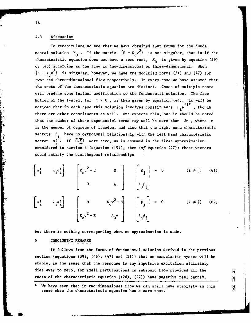
4.3 Discussion

To recapitulate we see that we have obtained four forms for the funda-

mental solution X0 If the matrix (E - Kav2) is not singular, that is if the

characteristic equation does not have a zero root, X0 is given by equation (39)

or (46) according as the flow is two-dimensional or three-dimensional. When

(E - Kyv2) is singular, however, we have the modified forms (51) and (47) for

two- and three-dimensional flow respectively. In every case we have assumed that

the roots of the characteristic equation are distinct. Cases of multiple roots

will produce some further modification to the fundamental solution. The free

motion of the system, for T > 0 , is then given by equation (44). It will be)Lit

noticed that in each case this solution involves constituents a.e , thoughi

there are other constituents as well. One expects this, but it should be noted

that the number of these exponential terms may well be more than 2n , where nis the number of degrees of freedom, and also that the right hand characteristic

vectors 8. have no orthogonal relationship with the left hand characteristic

vector a If E( ) were zero, as is assumed in the first approximation

considered in section 3 (equation (19)), then (of equation (27)) these vectors

would satisfy the biorthogonal relationships

a[! A.a! Kv2-E 0 [ ] = 0 (i j) (61)

0 A jXj

ac! A.ci!] 0 Kv 2 _ [E. 0 (i j) (62j

Kav-2_E A 0v

*I

but there is nothing corresponding when no approximation is made.

5 CONCLUDING REMARKS

It follows from the forms of fundamental solution derived in the previous

section (equations (39), (46), (47) and (51)) that an aeroelastic system will be

stable, in the sense that the response to any impulsive excitation ultimately

dies away to zero, for small perturbations in subsonic flow provided all the

roots of the characteristic equation ((26), (27)) have negative real parts*.

* We have seen that in two-dimensional flow we can still have stability in this

sense when the characteristic equation has a zero root.

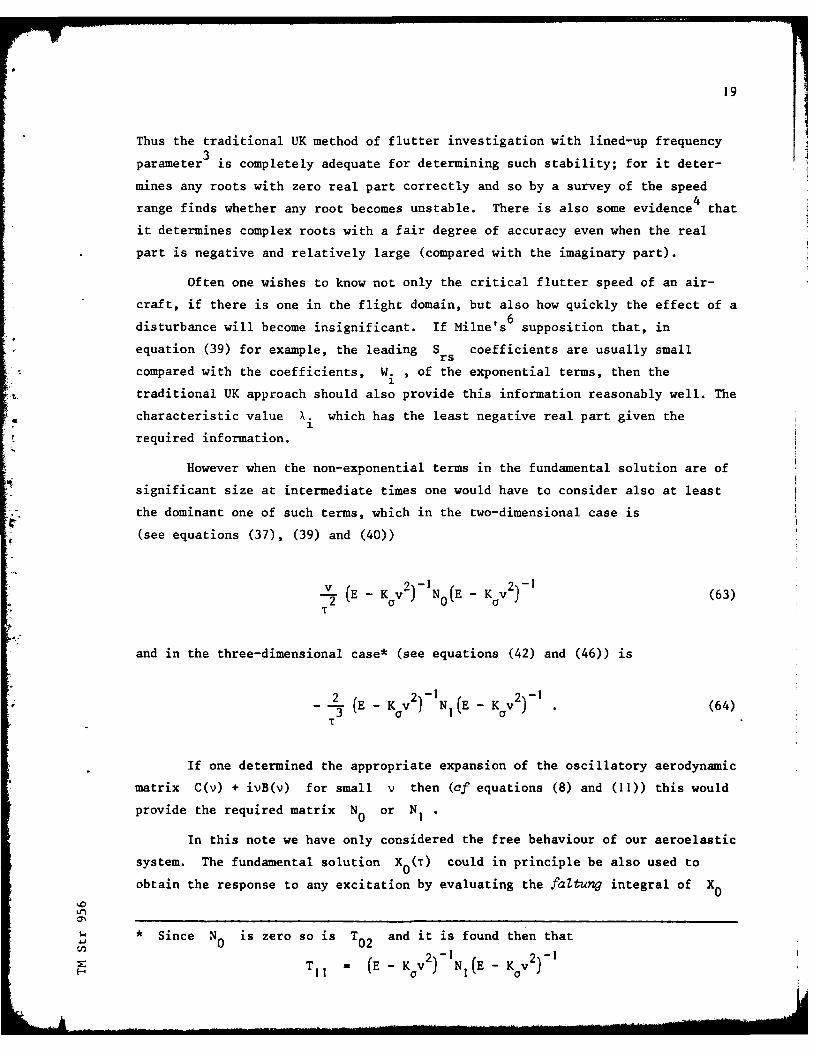
19

Thus the traditional UK method of flutter investigation with lined-up frequency

parameter3 is completely adequate for determining such stability; for it deter-

mines any roots with zero real part correctly and so by a survey of the speed4range finds whether any root becomes unstable. There is also some evidence that

it determines complex roots with a fair degree of accuracy even when the real

part is negative and relatively large (compared with the imaginary part).

Often one wishes to know not only the critical flutter speed of an air-

craft, if there is one in the flight domain, but also how quickly the effect of a

disturbance will become insignificant. If Milne's supposition that, in

equation (39) for example, the leading S coefficients are usually smallrs

compared with the coefficients, Wi , of the exponential terms, then the

traditional UK approach should also provide this information reasonably well. The

characteristic value X. which has the least negative real part given thei

required information.

However when the non-exponential terms in the fundamental solution are of

significant size at intermediate times one would have to consider also at least

the dominant one of such terms, which in the two-dimensional case is

(see equations (37), (39) and (40))

V (E - Kyv2 )- N0(E - Kyv2 )-I (63)2T

and in the three-dimensional case* (see equations (42) and (46)) is

-2 (E - Kv2-NI(E - Kv2 I (64)

If one determined the appropriate expansion of the oscillatory aerodynamic

matrix C(v) + ivB(v) for small v then (cf equations (8) and (11)) this would

provide the required matrix N or N .

In this note we have only considered the free behaviour of our aeroelastic

system. The fundamental solution X () could in principle be also used to

obtain the response to any excitation by evaluating the faltun integral of X0

Since N is zero so is T0 2 and it is found then that0 02 -

T1- (E - K v2) N(E Kv 2 )r0

20

in a form convenient for use at small T which we have not obtained. It wouldprobably therefore be advisable to determine first the Laplace transform of the

response and then invert that.

C1

r'

i.~0

21

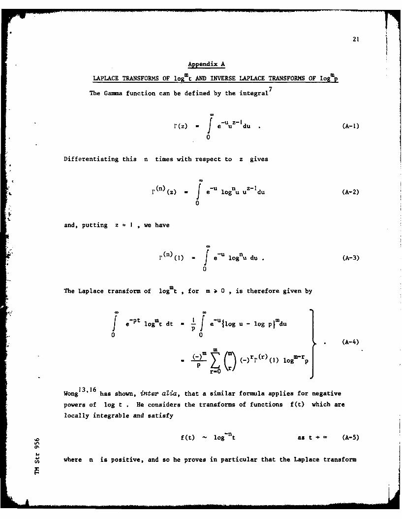
Appendix A

LAPLACE TRANSFORMS OF log t AND INVERSE LAPLACE TRANSFORMS OF logmp

The Gamma function can be defined by the integral7

r(z) I e-UuZ-ldu (A-1)

0

Differentiating this n times with respect to z gives

; (n) -U lon z-1r (z) = U uu du (A-2)

0

oand, putting z = I , we have

r(n)(1) f e- u lognu du . (A-3)

0

The Laplace transform of log t , for m o 0 , is therefore given by

e-pt logmt dt = f J'ulog u - log

0 0(A-4)

(-=m (Z ) (-)rr(r)(1) 1ogm-rp

r-OC

Wong 13,16 has shown, inter alia, that a similar formula applies for negative

powers of log t . He considers the transforms of functions f(t) which are

locally integrable and satisfy

f(t) _ log-nt as t (A-5)

U where n is positive, and so he proves in particular that the Laplace transform

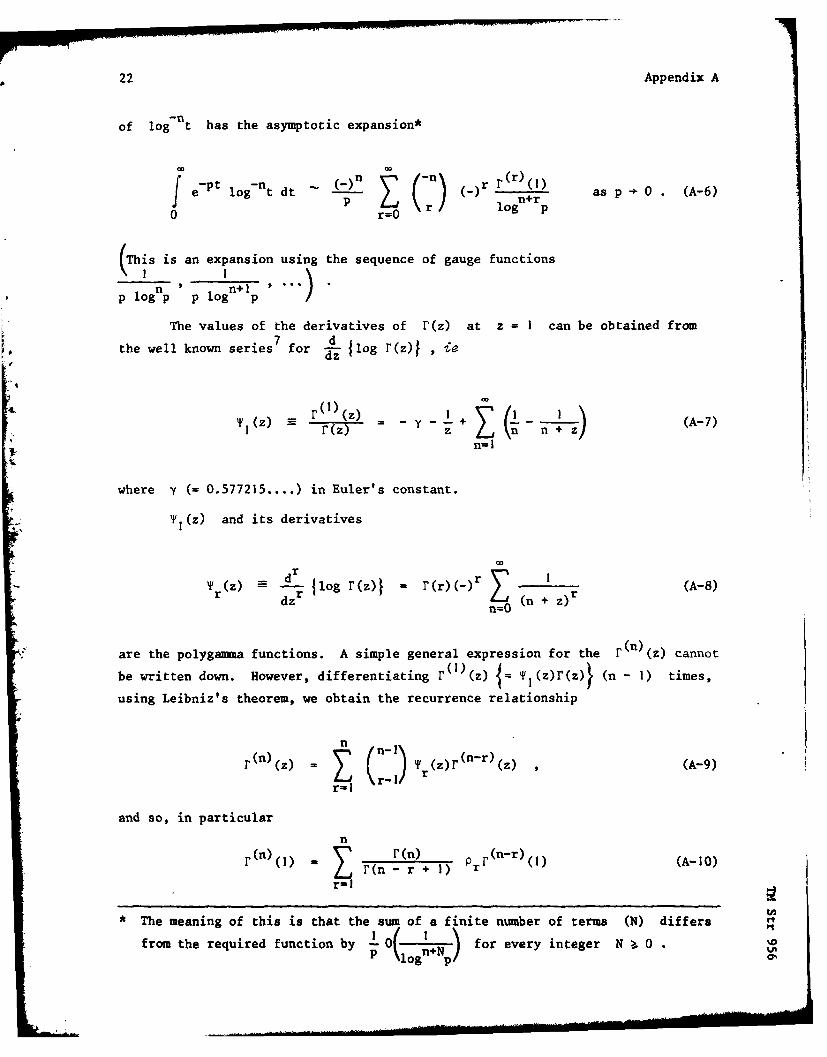
22 Appendix A

of log-n t has the asymptotic expansion*

e-Pt lognt dt - r) (r r(r)_L_ asp 0 (A-6)fP log n +r "

0 r=0 P

(This is an expansion using the sequence of gauge functionsI

p lognp p i og n+Tp

The values of the derivatives of r(z) at z = I can be obtained from

the well known series7 for j-z flog r(z)l ie

4

O

S(Z) r ) (z) - -I+ (A-7)r(z - = n-zJ

n= I

where Y (= 0.577215 ....) in Euler's constant.

TI (z) and its derivatives

T(z) = d Ilog r (z) 1 r (r) (-) r (A-8)r dz r Z (n + z) r

n=0

are the polygamma functions. A simple general expression for the r(n) (z) cannot

be written down. However, differentiating r(1)(z) I= T I(z)r(z) (n - 1) times,

using Leibniz's theorem, we obtain the recurrence relationship

rn(z) = Z -) r (r (Z) (A-9)r-I rZ

and so, in particular

nrn() 1)r(n) Or(n-r)(1) (A-10)

rEn)() r(n - ) r rr-|I

The meaning of this is that the sum of a finite number of terms (N) differs'(')o11

from the required function by 1 01on+N for every integer N >, 0Tlog pI

Appendix A 23

where PI = rI Y(-l

and

P ' r~ orZ (r 2). (A- 12)r r (r)- r

S=I s

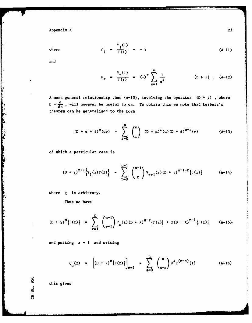
A more general relationship than (A-10), involving the operator (D + X) ,where

=d.9 D = -- , will however be useful to us. To obtain this we note that Leibniz's

theorem can be generalised to the form

(D + a+ )(uv) = ) (D + iru(D + 8)r()(A-13)

raO r

of which a particular case is

(D + X) n-I T ( r(Z)4 T ~ )(z)(D + X)n-lr jr(z)l (A-14)r=OI

where X is arbitrary.

Thus we have

(D+ X)nlr(z), E C (:: ri'(z)(D + X)n-r r(z)l + X(D + X)nI jr(z4l (Amr= I

and putting z -I and writing

&(x) - [D + X) n r(z)I] n ()n xsr (I)) (A- 16)

gin

ai this gives

Wn

24 Appendix A

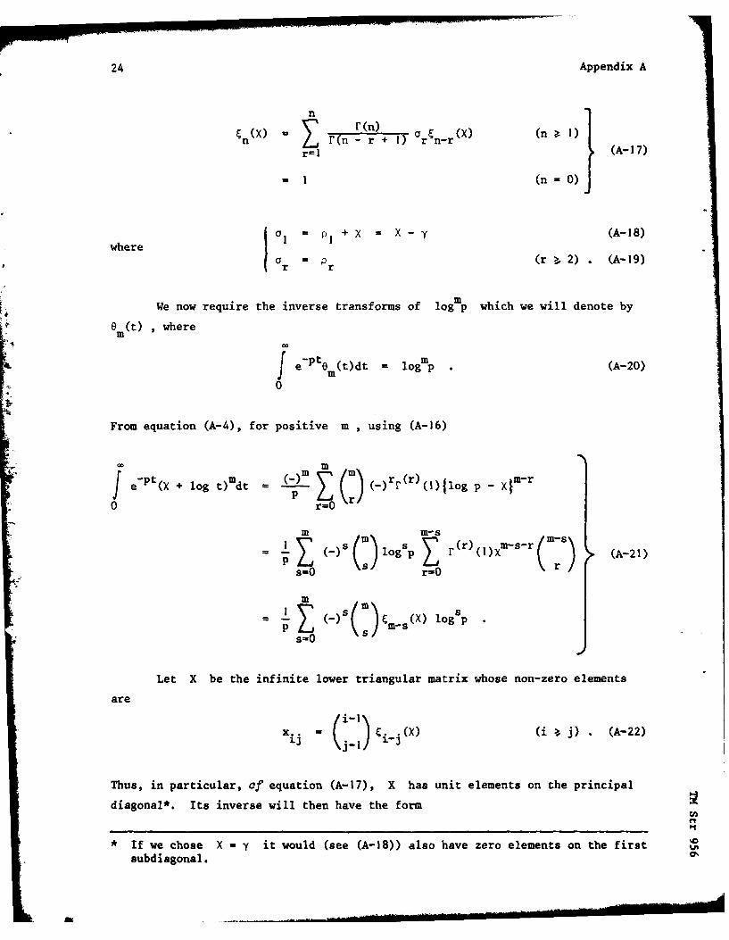
n *r(n) (x) (n 1)n~ X r(n - r + IT ar n-r

rffil (A-1 7)

= 1 (n =0)J

where a = P1 + X X - Y (A-18)

ar = Pr (r > 2) . (A-19)

We now require the inverse transforms of logmp which we will denote bye (t) ,where

mm f , e-Pt 6m (t)dt filogmp (A-20)

0

From equation (A-4), for positive m , using (A-16)CO MePt(X + log t)mdt = H (:) (_)rr(r)(,)llog p x-

0 r=

m m-s21

s-0 rr

- L~(_)s() m~s(X) log p

Let X be the infinite lower triangular matrix whose non-zero elements

are

x.. = () Wi-(X) (i , j) . (A-22)

Thus, in particular, of equation (A-17), X has unit elements on the principal

diagonal*. Its inverse will then have the form

* If we chose X - Y it would (see (A-18)) also have zero elements on the first

subdiagonal.

Appendix A 25

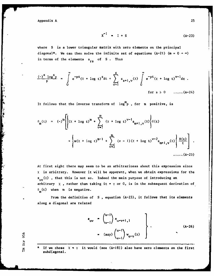
x- I + S (A-23)

where S is a lower triangular matrix with zero elements on the principal

diagonal*. We can then solve the infinite set of equations (A-21) (m f 0 -)

in terms of the elements s of S . Thusrs

)s lg Sp =f ePt(X + log t)sdt + s () e-Pt(U + log t)V- dtp jSs+l •

0 v=l 0

for s > 0 ..... (A-24)

mIt follows that the inverse transform of log p , for m positive, is

m(t) ()m [(X + log t)m + (X + log t)v- lsm+ ,,v (X) 6(t)

+ )m(X + log t)m -I + Z (v 1)(X log tv-2

v=2

..... (A-25)

At first sight there may seem to be an arbitrariness about this expression since

x is arbitrary. However it will be apparent, when we obtain expressions for the

Suv (X) , that this is not so. Indeed the main purpose of introducing an

arbitrary x , rather than taking it = y or 0, is in the subsequent derivation of0 (t) when m is negative.m

From the definition of S , equation (A-23), it follows that its elements

along a diagonal are related

Su -1 Su-v+i0i

(A-26)

U,-Ln- (say) w Wa v-i)u

• If we chose X - Y it would (see (A-18)) also have zero elements on the first

subdiagonal.

26 Appendix A

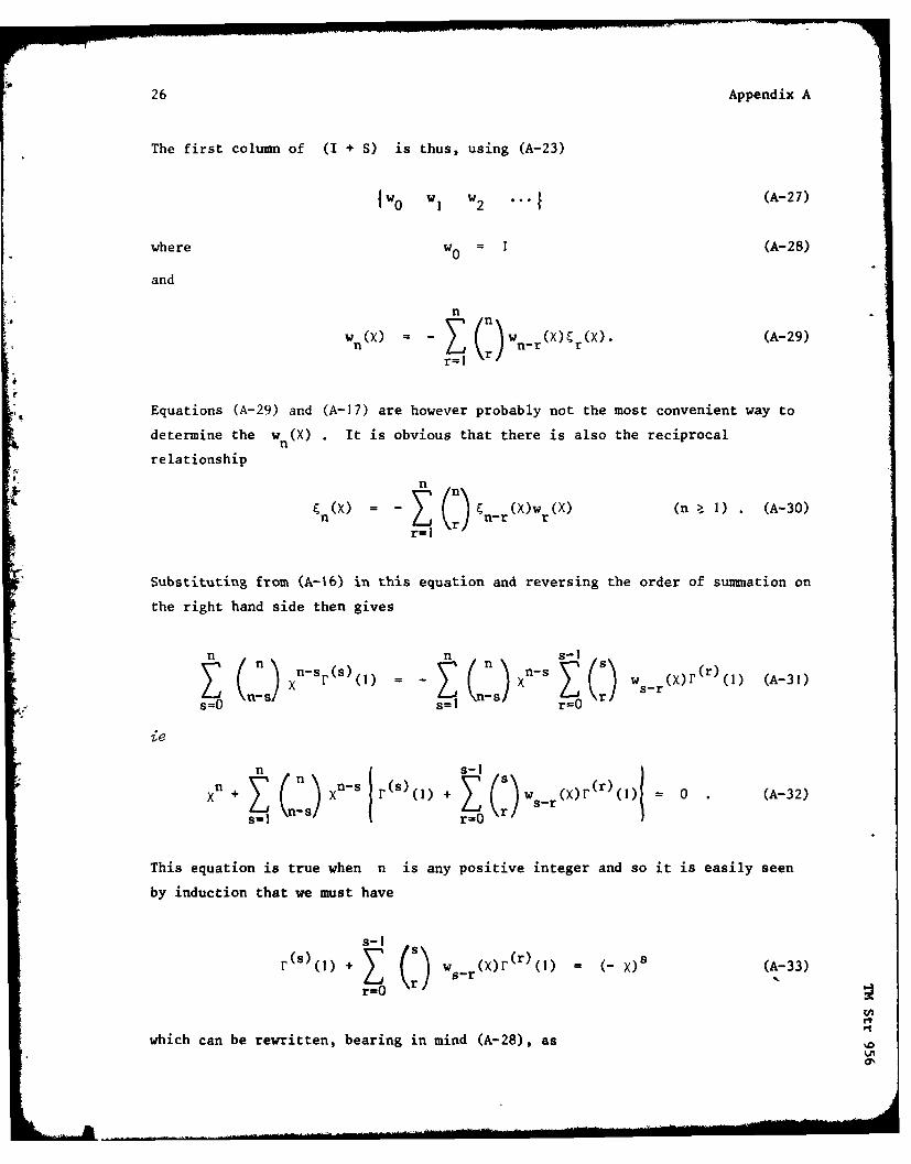
The first column of (I + S) is thus, using (A-23)

1w0 w1 w2 ... (A-27)

where w0 = I (A-28)

and

n

(x W ()w- r(x). (A-29)rrr=l

Equations (A-29) and (A-17) are however probably not the most convenient way todetermine the w (X) . It is obvious that there is also the reciprocal

n

relationshipn

n(x) = - (n) Cn:(X)Wr( ) (n I) (A-30)

r=1

Substituting from (A-16) in this equation and reversing the order of summation on

the right hand side then gives

n)Xn-sr (s) ( - xn- s Ws(x)r(r)( 1) (A-31)

Ss=l r=0

je

sn-s IrX(() + E (s)ws rr rI = 0 (A-32)

This equation is true when n is any positive integer and so it is easily seen

by induction that we must have

S-I

r (s)(1)+ z (s)wsr(X)r(r)()= (- X)s (A-33)

r=0 \r

which can be rewritten, bearing in mind (A-28), ask. 2,

Appendix A 27

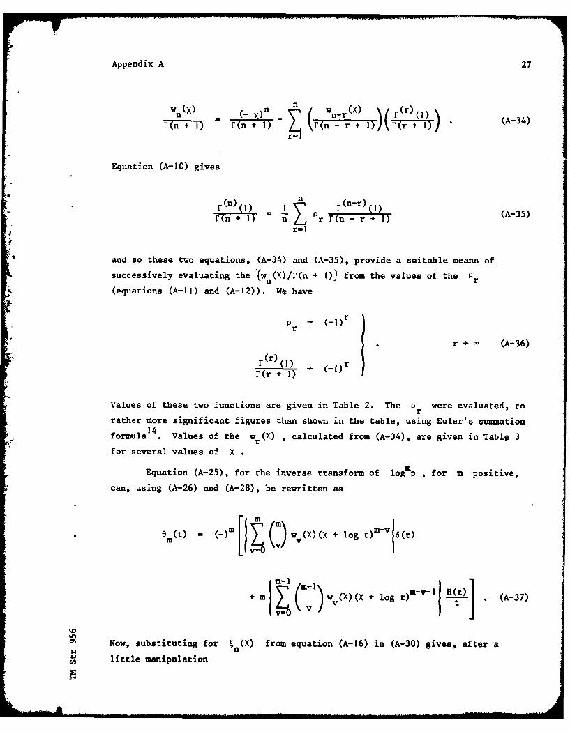
wnx W X- x-r r r (A-34)r~n + 1) r(n + I) L r(n-r + 1))\r(r + I)

Equation (A-10) gives

r(n)( n r(n-r))

r(n + 1) nl Z r r(n - r + 1) (-5

and so these two equations, (A-34) and (A-35), provide a suitable means of

successively evaluating the '(w n(x)/r'(n + I)from the values of the P r

(equations (A-1l) and (A-12)). We have

*+ ( rr

r CO (A-36)

r(r)rr (r + TY

Values of these two functions are given in Table 2. The p rwere evaluated, to

rather more significant figures than shown in the table, using Euler's summation14formula . Values of the w r(X) , calculated from (A-34), are given in Table 3

for several values of X

mEquation (A-25), for the inverse transform of log p , for m positive,

can, using (A-26) and (A-28), be rewritten as

em(t) - (-m[E Z)wO (X)(x + log tOm-v 6(t)

+ m) (In2I)W () + log 0)M-v I~ 1(t)] (-7

Now, substituting for M X from equation (A-16) in (A-30) gives, after an

CA little manipulation

28 Appendix A

ns

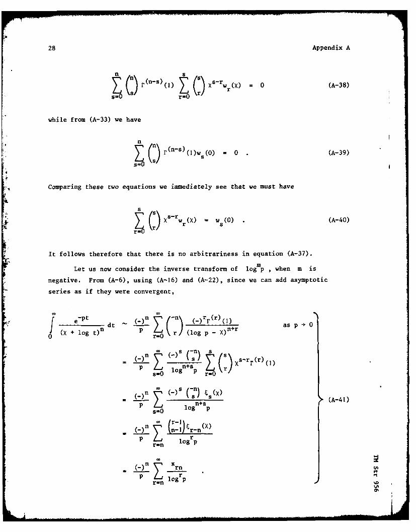
SM (: r (n-s) () (:) X sr w r(W 0 (A-38)r=O

while from (A-33) we have

n

T, (:) r(n-s) (Ow (0) =0 (A-39)S=O

Comparing these two equations we iunnediately see that we must have

s-

(s -wr(X) uws(0) .(A-40)

It follows therefore that there is no arbitrariness in equation (A-37).

Let us now consider the inverse transform of log p , when m is

negative. From (A-6), using (A-16) and (A-22), since we can add asymptotic

series as if they were convergent,

e-Pt dt ()nz (n (_)rr(r)(I) as p 0

0 (X + log t)n -rJ (log p - X)n+ r

r=O

= s log n+s p C) Xs r(()

M E n+s (A-41)

s=O log p

H n l ) r-n (x)

r r-n log pr

r logrp

Appendix A 29

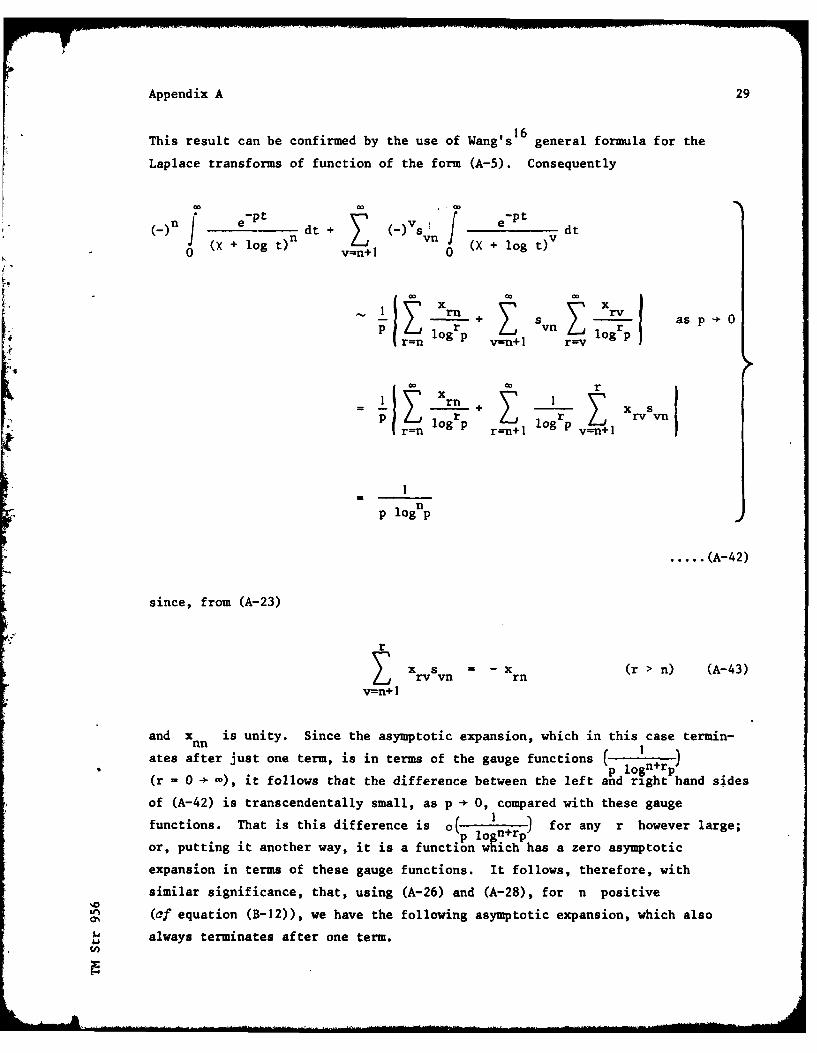
16This result can be confirmed by the use of Wang's general formula for the

Laplace transforms of function of the form (A-5). Consequently

()e -p t v e-P tdt+ - -Svn dt

0 (X + log t)n vn+1 0 (X + log t)v

Xrn + s ras p *0

P ogrp Zvn rp= V n+1 r=v lo p

I X~rn+1p orp 0grp Z Xrvvn

p lognp

..... (A-42)

since, from (A-23)

r

XrvSvn Xrn (r > n) (A-43)

and Xnn is unity. Since the asymptotic expansion, which in this case termin-

ates after just one term, is in terms of the gauge functions (p 1on+r )(r - 0 - -), it follows that the difference between the left and right hand sides

of (A-42) is transcendentally small, as p - 0, compared with these gauge

functions. That is this difference is o( 1 . -) for any r however large;p ptingrp

or, putting it another way, it is a function which has a zero asymptotic

expansion in terms of these gauge functions. It follows, therefore, with

similar significance, that, using (A-26) and (A-28), for n positive

n (of equation (B-12)), we have the following asymptotic expansion, which also

8 always terminates after one term.

30 Appendix A

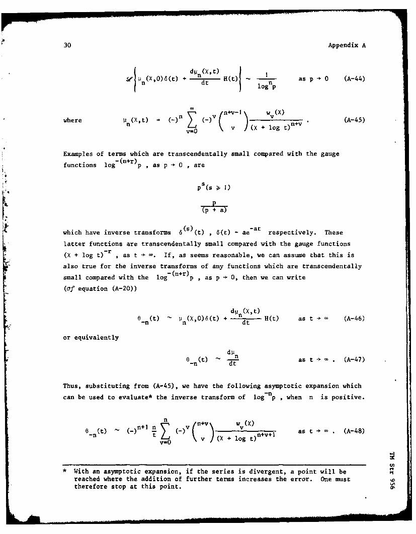
' n (X '0 ) d(t ) + dt H(t) I as p - 0 (A-44)lognp

where 1n (X,t) = (_)n 0()v ) v M (A-45)nvE=0 (X + log t)n +v

Examples of terms which are transcendentally small compared with the gauge-(n+r)

functions log p , as p 0 , are

Sp (s > I)

P(p + a)

(S) -atwhich have inverse transforms 6 (t) , 6(t) - ae respectively. These

latter functions are transcendentally small compared with the gauge functions

(X + log t)- r , as t . If, as seems reasonable, we can assume that this is

also true for the inverse transforms of any functions which are transcendentally

small compared with the log- (n+r)p , as p , 0, then we can write

(cf equation (A-20))

d~n(X,t)

e-n(t) n (X,0)6(t) + dt H(t) as t (A-46)

or equivalently

diin(t) - as t . (A-47)-n dt

Thus, substituting from (A-45), we have the following asymptotic expansion which

can be used to evaluate* the inverse transform of log-n p , when n is positive.

n(t) n n n Hn ++vl tv( as t (x8(X + log t)n+v+1

-n- v-O

* With an asymptotic expansion, if the series is divergent, a point will be

reached where the addition of further terms increases the error. One musttherefore stop at this point.

Appendix A 31

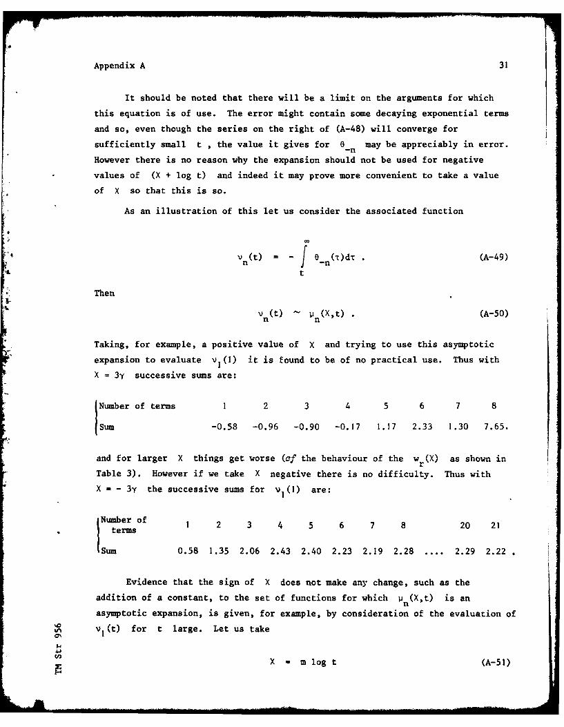
It should be noted that there will be a limit on the arguments for which

this equation is of use. The error might contain some decaying exponential terms

and so, even though the series on the right of (A-48) will converge for

sufficiently small t , the value it gives for e may be appreciably in error.-n

However there is no reason why the expansion should not be used for negative

values of (X + log t) and indeed it may prove more convenient to take a value

of X so that this is so.

As an illustration of this let us consider the associated function

V n(t) ffi (-_ )dT. (A-49)

t

Then

Vn (t) n(Xt) . (A-50)

Taking, for example, a positive value of X and trying to use this asymptotic

expansion to evaluate v (1) it is found to be of no practical use. Thus with

X = 3y successive sums are:

Number of terms 1 2 3 4 5 6 7 8

Sum -0.58 -0.96 -0.90 -0.17 1.17 2.33 1.30 7.65.

and for larger X things get worse (of the behaviour of the w r(X) as shown in

Table 3). However if we take X negative there is no difficulty. Thus with

X = - 3y the successive sums for v1 (1) are:

INumber of 1 2 3 4 5 6 7 8 20 21terms

Sum 0.58 1.35 2.06 2.43 2.40 2.23 2.19 2.28 .... 2.29 2.22

Evidence that the sign of X does not make any change, such as theaddition of a constant, to the set of functions for which pn (X,t) is an

asymptotic expansion, is given, for example, by consideration of the evaluation of

n Vl(t) for t large. Let us take

X = m log t (A-51)

32 Appendix A

where m is any number, positive or negative, othe- than -I such that 1XI will

also be large. Then, when that is so (Of equation (A-34)) we have

W v(X) -X) v (A-52)

It is then easily seen that the sum, of N terms of the series for p (X't)

equation (A-45), and hence of the asymptotic expansion for v (t) , is

Vl(t ) (X,t 0 oI (A-53)

Thus we ultimately get the same value whether m is positive or negative (orindeed zero, as (A-45) and Table 3 show) provided m < I

We have thus established the validity of our expression (A-48) for the

inverse transform of lognp when n is a negative integer. It should perhaps

be noted that we have there an infinity of asymptotic expansion, for the para-

meter X is arbitrary. For n positive we had previously obtained the

expression (A-37) - again containing an arbitrary parameter X . To complete the

picture we have the well known fact that

0(t) = 6(t) (A-54)

it being the function whose Laplace transform is I.

A particular case which we require in tbe main part of the Memorandum is

that when n = I which from (A-37) is

S(t) = - (y + log t)(t) H(t) (A--55)t

33

Appendix B

THE RIGHT HAND DIRAC DELTA FUNCTION ANDITS USE IN LAPLACE TRANSFORM THEORY

Since the Laplace transform integral has a lower limit of zero one has to

use what is called a right hand Dirac delta function 6(t) which is defined to

be such that

d(n)(O

n 0 co (B-I)

6(n) 0

J6(-r)f(T)dr f(O)H(t) (B-2)

0

H(t) =0 t <

where (B-3)

and f(t) is a fairly good functioln1

It follows that we can write

6(t) = dHi(t) (B-4)dt

for

J (T dH('r) dT = [fT)HcT)]t -fdf(r) HTd

0 0

M H(tOf(t) - f( d T

0+(B-5)

M H(t)f(O) + JH(t) - Iff(t) -(~

C - H(t)f(O).

34 Appendix B

Differentiating (B-2) we see also that 6(t) is such that

6(t)f(t) = 6(t)f(O). (B-6)

For the derivatives of 6 we have, integrating by parts and using (B-1),

L n-Ij 6(n)(T)f(T)dT = (_)rf(r),() (n-l-r)(t) + (_)nf(n)(o)Ht)

0 r=O

Also, from (B-6), by successive differentiation*

n

6 (n) (t)f(t) (n) r6 (n-r) (t)f(r)(0) (B-8)

r=O

and so (B-7) can be rewritten as**

t n I n \ ,J 6 (n) (T)f(T)dT -n-I n-1 n )()r 6 (r(t)f(n-l-r)(o) + (-)nf(n)(O)H(t)

0 r

..... (B-9)

It follows from (B-2) and (B-9), putting f(T) - e- p T , t = , and using

(B-1), that the Laplace transforms of the 6 functions are

(n)j e-Pt6(n)(t)dt = pn n = 0 .(B-10)

0

Consequently, from the well known theorem for the inverse transform of a product,

we find that, using (B-9) and (B-7), for n > I

* Incidentally putting t - 0 in (B-8), we notice that this equation would not

be satisfied if the first of the conditions (B-I) in the definition of 6 were

relaxed.n-l-r f~ )nr

** We have used the fact that n n

s s=O r+i U's...

4

Appendix B 35

t

=p f (t - r) 6 (n) (Tr)dT

n-1 (n--r n

6 (r) f( 6 () (t) + fn (t)H(t) (B-1l)

n-I

= fi f(r)(0)(n-l-r) (t) + f (n)(t)H(t)

The particular case n = I is the well known formula

p f(f (t(t) H(t) + f (0) 6(t) (B-12)

which can be written, using (B-10), as

P ,, f (t) - f(O) - {e( l)W(t4 (B-13)

In practice one may well obtain as an inverse transform a function in the

form of an infinite series of terms, containing the 6 function and its

derivatives. At the two limits t - 0, - such a function is by definition zero,

but how do we interpret it elsewhere? Consider for example the function

t ( - ) s ( S ) ( t ) ( (a) > 0) (B-14)X(t) ,- Zs+l

s-O a

-at

which has the same Laplace transform as e- at for p > 0. Lerch's theorem states

that if two functions have the same Laplace transform then their difference is a

null function*. Thus for this example we require therefore that

S{eaT - X(T)}dT 1 - e-at + X(t) - H(t) (B-15)

0%0

It

* A null function is one whose J is zero for t >. 0.

0

36 Appendix B

should be zero for all t > 0. Thus we must have

X(t) = e-at t > 0

(B-16)

-0 t= 0

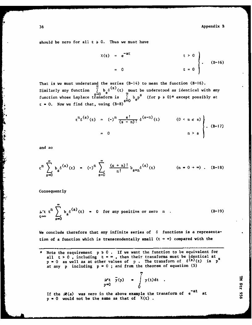
That is we must understand the series (B-14) to mean the function (B-16).

Similarly any function b 6(s(t) must be understood as identical with anyS=0

function whose Laplace transform is 0 b p5 (for p 0)* except possibly at

t = 0. Now we find that, using (B-8)

= n S! 6(s-n)(t) (0 < n < s)(s n)!

(B-17)

=0 n > s

and so

tn E bs(S)(t) (_)n I (s + n) b (s) (t) (n 0 (B-18)kj n! s+n =~+o) (-8

s=0 s=0

Consequently

't tn b,6(s)(t) = 0 for any positive or zero n (B-19)

t- o ZJ

We conclude therefore that any infinite series of 6 functions is a representa-

tion of a function which is transcendentally small (t - -) compared with the

• Note the requirement p > 0 If we want the function to be equivalent forall t > 0 , including t - , then their transforms must be identical at sp 0 as well as at other values of p . The transform of 6(s)(t) is pat any p including p - 0 ; and from the theorem of equation (5)

Yt y(p) = f y(t)dtP+° 0

-atIf the R(a) was zero in the above example the transform of e at 'p -0 would not be the same as that of X(t)

Appendix B 37

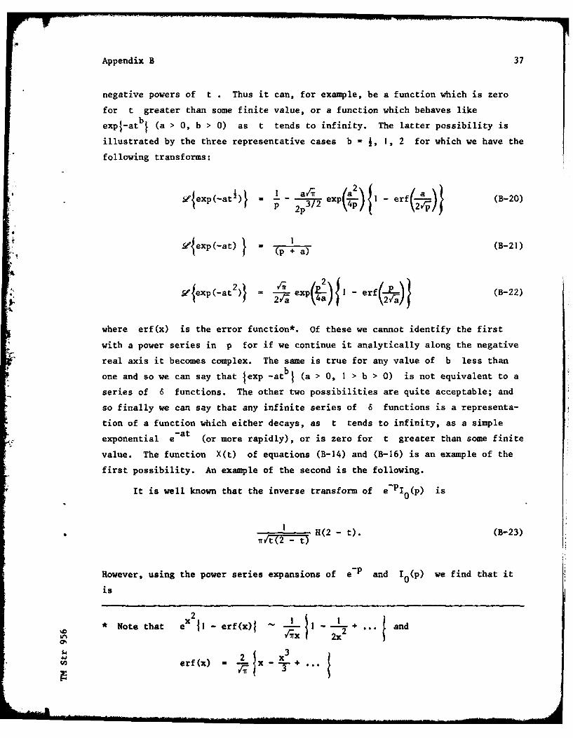
negative powers of t . Thus it can, for example, be a function which is zero

for t greater than some finite value, or a function which behaves like

expl-atb I (a > 0, b > 0) as t tends to infinity. The latter possibility is

illustrated by the three representative cases b 1 , I, 2 for which we have the

following transforms:

sexpC-ad)} I aA~ a2 1 erf (B-20)P 2p3' 4pP 1

jexp(-at) + a)-21)

x 1- exp )I - erf (B-22)

where erf(x) is the error function*. Of these we cannot identify the first

with a power series in p for if we continue it analytically along the negative

real axis it becomes complex. The same is true for any value of b less than

one and so we can say that Iexp -at b (a > 0, 1 > b > 0) is not equivalent to a

series of 6 functions. The other two possibilities are quite acceptable; and

so finally we can say that any infinite series of 6 functions is a representa-

tion of a function which either decays, as t tends to infinity, as a simple

exponential e-a t (or more rapidly), or is zero for t greater than some finite

value. The function X(t) of equations (B-14) and (B-16) is an example of the

first possibility. An example of the second is the following.

It is well known that the inverse transform of e-PI0 (p) is

H(2 - ). (B-23)(- t)

However, using the power series expansions of e- p and I0 (p) we find that it

is

2I* Note that ex I1 - erf(x)l 9-li --- 2+ and

2x2 " )"

erf(x) = . x - + ...

.. .. . . ..3l .. . . I I I RI

* 38 Appendix B

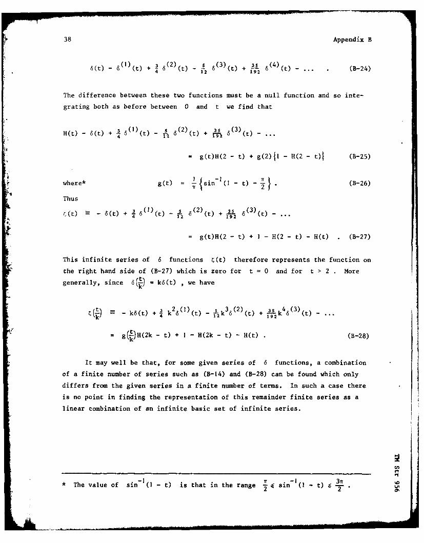
6(t) - 60)(t) + 2 6 (2)(t) 2 (3)(t) + 3S 6(4)(t) " (B-24)

The difference between these two functions must be a null function and so inte-

grating both as before between 0 and t we find that

H(t) - 6(t) + - (t) - A 6( 2 )(t) + 192 63(t) -

- g(t)H(2 - t) + g(2)11 - H(2 - t)[ (B-25)

r where* g(t) = sin- (I - t) (B-26)

Thus

(t) - 6(t) + * 6(1(t) - 6(2) (t) + -L- 6< 3 (t) -

= g(t)H(2 - t) + I - H(2 -t) -H(t) . (B-27)

This infinite series of 6 functions C(t) therefore represents the function on

the right hand side of (B-27) which is zero for t = 0 and for t > 2 . More

generally, since 6 .) - k6(t) , we have

k6(t) + 2 k 2 6( 1 ) (t) k3 6 (2) (t) + -1 k 4 6 (3) (t)

= g(k)H(2k - t) + I - H(2k - t) - H(t) (B-28)

It may well be that, for some given series of 6 functions, a combination

of a finite number of series such as (B-14) and (B-28) can be found which only

differs from the given series in a finite number of terms. In such a case there

is no point in finding the representation of this remainder finite series as a

linear combination of an infinite basic set of infinite series.

31rtThe value of sin( t) is that in the range sin

39

Table I

APPROXIMATE VALUES OF Er(p) K1 (k)/t K(P2-) + K 1 P)

Real negative Real positive Purely imaginaryp p p

Wx ix)

0 111

0.1 1.1241 0.4753i 0.8024 0.8319 TO.1723i

0.2 0.7677 0.7371i 0.7315 0.7276 T0.1886i

0.3 0.4605 0.6368i 0.6901 0.6650 TO.1793i

0.4 0.3240 0.4781i 0.6622 0.6250 T0.1650i

0.5 0.2768 0.3536i 0.6418 0.5979 T0. 1507i.

0.6 0.2672 0.2647i 0.6263 0.5788 T0.1378i

0.7 0.2731 0.2012i 0.6139 0.5648 T0.1264i

0.8 0.2798 T0.1550i 0.6039 0.5541 T0.1165i

0.9 0.2959 T0.1207i 0.5955 0.5459 T0.1078i

1.0 0.3141 T0.09482i 0.5884 0.5394 T0.1003i

2 0.4110 T0.01063i. 0.5512 0.5130 T0.05769i

3 0.4475 T0.001360i. 0.5362 0.5063 T0.04000i

4 0.4634 T0.0001794i. 0.5280 0.5037 T0.03050i

5 0.4718 ;0.00002393i. 0.5229 0.5024 4:0.02460i

10 0.4868 T0.0 .......i 0.5199 0.5006 T0.01245i

0.5 0.5 0.5

LM

Qf

40

Table 2

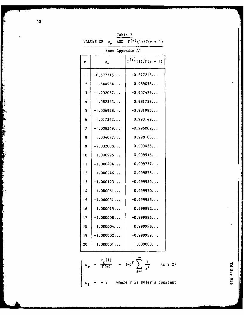
VALUES OF r AND r(r)(1)/r(r + 1)

(see Appendix A)

r Pr r)(1)/r(r + 1)

1 -0.577215... -0.577215...

2 1.644934... 0.989056...

3 -1.202057... -0.907479...

4 1.082323... 0.981728...

5 -1.036928... -0.981995...

6 1.017343... 0.993149...

7 -1.008349... -0.996002...

8 1.004077... 0.998106...

9 -1.002008... -0.999025...

10 1.000995... 0.999516...

11 -1.000494... -0.999757...

12 1.000246... 0.999878...

13 -1.000123... -0.999939...

14 1.000061... 0.999970...

15 -1.000031... -0.999985...

16 1.000015... 0.999992...

17 -1.000008... -0.999996...

18 1.000004... 0.999998...

19 -1.000002... -0.999999...

20 1.000001... 1.000000...

r (1) H r (r 2)r (r

1 - 7 where y is Euler's constant

41

N cc o ~

44-j

o 6

N 03N 4 o N to

0~~~* N cc NNX N7 79 Ff

go4 .4 9

Il ID ID 'ar

.0 04 m 0 0 L

0

No 44 w.r4 * 8

9 ON a, N N

I 4J4

140

42

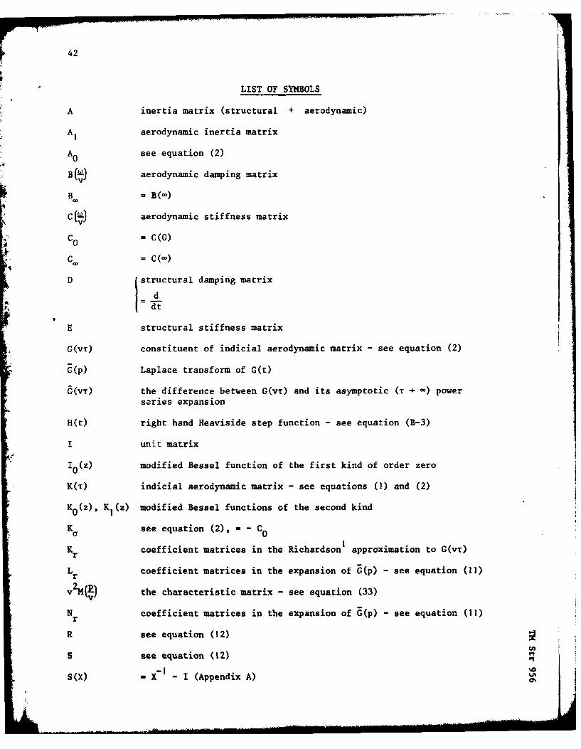
LIST OF SYMBOLS

A inertia matrix (structural + aerodynamic)

A| aerodynamic inertia matrix

A0 see equation (2)

aerodynamic damping matrixB()

B = B(-)

C( ) aerodynamic stiffness matrix

Co = C(O)

c = c (0)

D (structural damping matrix

d

E structural stiffness matrix

G(vT) constituent of indicial aerodynamic matrix - see equation (2)

G(p) Laplace transform of G(t)

G(vT) the difference between G(VT) and its asymptotic (T 0) powerseries expansion

H(t) right hand Heaviside step function - see equation (B-3)

I unit matrix

I (Z) modified Bessel function of the first kind of order zero

K(T) indicial aerodynamic matrix - see equations (1) and (2)

Ko(z), K1 (z) modified Bessel functions of the second kind

Ka see equation (2), - - C00I

Kr coefficient matrices in the Richardson approximation to G(vT)

L coefficient matrices in the expansion of 6(p) - see equation (II)' r

vlm() the characteristic matrix - see equation (33)

N coefficient matrices in the expansion of G(p) - see equation (11)

r

R see equation (12)

S see equation (12) '

S(X) mX 1 - I (Appendix A)

43

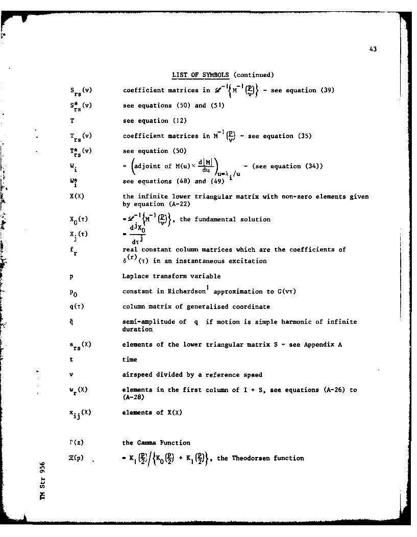
LIST OF SYMBOLS (continued)

S (V) coefficient matrices in 9 -I11-I(W - see equation (39)rs I vJ

S* (v) see equations (50) and (51)rs

T see equation (12)

Trs (v) coefficient matrices in M-lv2) - see equation (35)

T* (v) see equation (50)rs

= (adjoint of M(u)x dIi)u - (see equation (34))I =./uW.* see equations (48) and (49) 11

X(X) the infinite lower triangular matrix with non-zero elements givenby equation (A-22)

XO(T)the fundam l solution

X. (T) ----=i dT i

f real constant column matrices which are the coefficients of

Sr(T)" in an instantaneous excitation

p Laplace transform variable

P0 constant in Richardson I approximation to G(vT)

q(T) column matrix of generalised coordinate

semi-amplitude of q if motion is simple harmonic of infiniteduration

Srs(X) elements of the lower triangular matrix S - see Appendix A

t time

v airspeed divided by a reference speed

w (X) elements in the first column of I + S, see equations (A-26) tor (A-28)

x. (X) elements of X(X)

r(z) the Gama Function

Z(p) - + the Theodorsen function

0% (4).42

44

LIST OF SYMBOLS (continued)

cz. left hand characteristic vector1

(rs)a u see equation (43)

Bi right hand characteristic vector

y 0.577215... , Euler's constant

6(t) right hand Dirac delta function, see Appendix B

6 (n) W dn6

dtC(t) see equation (B-23)

r see equation (29)

nr see equation (29)

rme em~ W -I ogmp)

characteristic value

11n see equations (A-44) and (A-45)

V= t/v, frequency parameter

(X) [D + x)nlr(z)l]

P (r 2)

I

r = pr (r r 2)

* time multiplied by (reference speed/reference length)X arbitrary constant used in getting inverse Laplace transform of

logmp, see Appendix A

X(t) see equation (B-14)

'Y (z)dr dVr Wlog (z) , the Polygamma functionsr z

frequency multiplied by (reference length/reference speed)

Wif(t)I - Laplace transform of f(t)

- inverse Laplace transform of f(p)

c.I'0U'n

45

LIST OF SYMBOLS (concluded)

() - n'/ r!(n r)f(n) d nf

f (x) -dx

.9(x)signifies the imaginary part of x

g(x) signifies the real part of x

LM

46

REFERENCES

No. Author Title, etc

I J.R. Richardson A more realistic method for routine flutter

calculations.

AIAA Symposium of Structural Dynamics and

Aeroelasticity (1965)

2 R.D. Milne Asymptotic solutions of linear stationary integro-

differential equations.

ARC R & M 3548 (1966)

3 A. Jocelyn Lawrence Comparison of different methods of assessing the

k P. Jackson free oscillatory characteristics of aeroelastic

systems.

ARC CP 1084 (1970)

4 D.L. Woodcock Further comparisons of different methods of assessing

A. Jocelyn Lawrence the free oscillatory characteristics of aeroelastic

systems.

RAE Technical Report 72188 (1972)

5 C.G.B. Mitchell Calculation of the response of a flexible aircraft to

harmonic and discrete gusts by a transform method.

RAE Technical Report 65264 (1965)

* 6 R.D. Milne The role of flutter derivatives in aircraft stability

and control.

AGARD Stab lity and Control Symposium, Cambridge

(1966)

7 E.T. Whittaker A course of modern analysis.

G.N. Watson p 241, Cambridge University Press (1946)

8 E.T. Copson An introduction to the theory of functions of a

complex variable.

p 119, Oxford University Press (1935)

9 H. Lomax Indicial aerodynamics.

AGARD Manual on Aeroelasticity, Vol II, Chapter 6

(1960)

10 H.C. Garner Asymptotic expansion for transient forces from quasi-

R.D. Milne steady subsonic wing theory.I

Aeronaut. Quart. Vol 17 (1966)

47

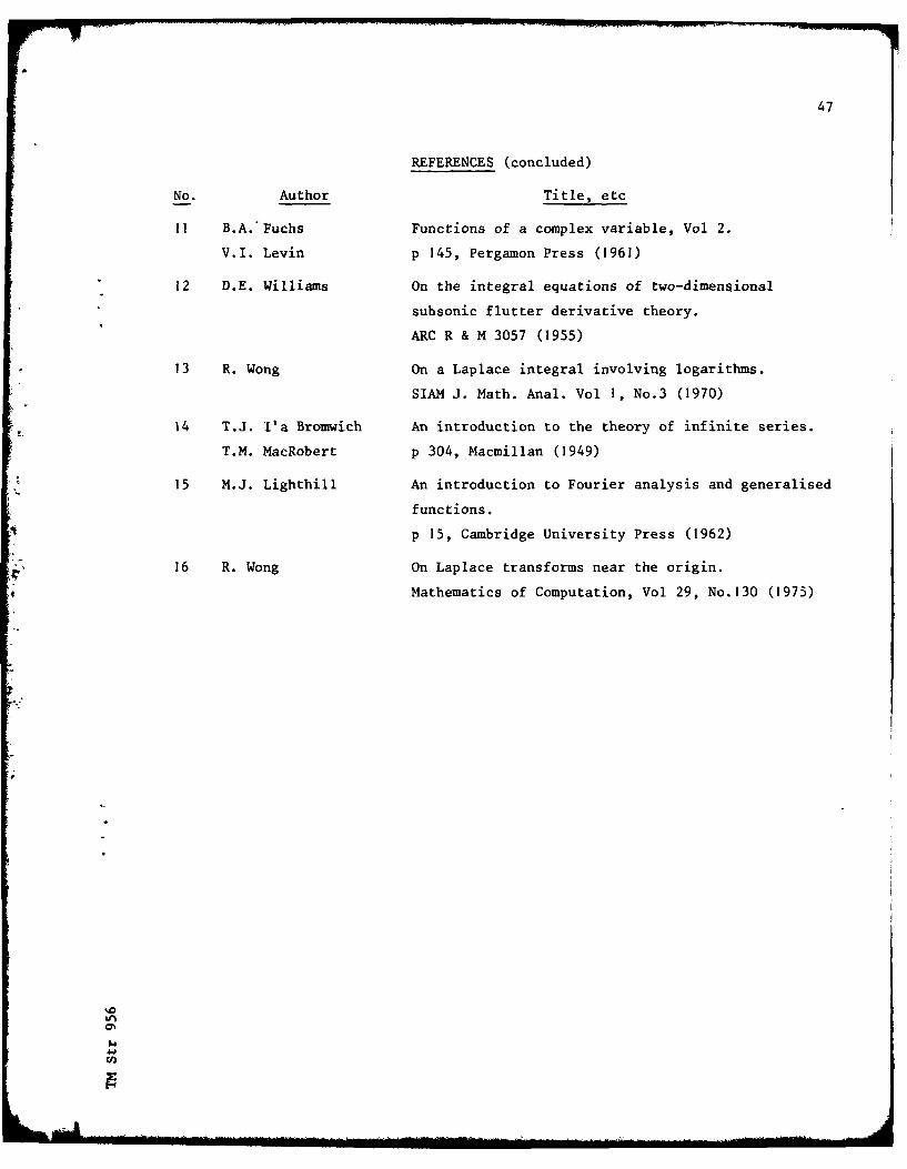
REFERENCES (concluded)

No. Author Title, etc

11 B.A.'Fuchs Functions of a complex variable, Vol 2.

V.I. Levin p 145, Pergamon Press (1961)

12 D.E. Williams On the integral equations of two-dimensional

subsonic flutter derivative theory.

ARC R & M 3057 (1955)

13 R. Wong On a Laplace integral involving logarithms.

SIAM J. Math. Anal. Vol 1, No.3 (1970)

14 T.J. I'a Bromwich An introduction to the theory of infinite series.

T.M. MacRobert p 304, Macmillan (1949)

15 M.J. Lighthill An introduction to Fourier analysis and generalised

functions.

p 15, Cambridge University Press (1962)

16 R. Wong On Laplace transforms near the origin.

Mathematics of Computation, Vol 29, No.130 (1975)

irn

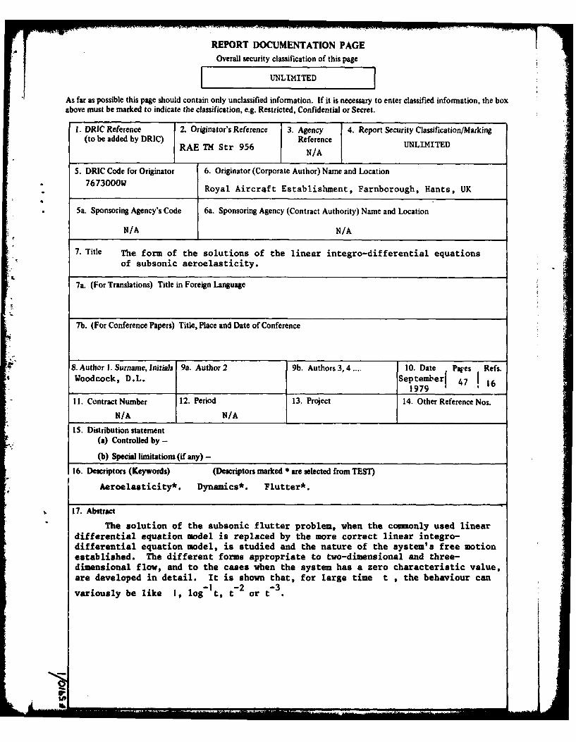
REPORT DOCUMENTATION PAGE

Overall security classification of this page

UNLIMITED

As far as possible this page should contain only unclassified information. If it is necessary to enter classified information, the boxabove must be marked to indicate the classification, e.g. Restricted, Confidential or Secret.

1. DRIC Reference 2. Originator's Reference 3. Agency 4. Report Security Classification/Marking(to be added by DRIC) Reference UNLIMITEDRAE TM Str 956 N/AMTE

N/A

5. DRIC Code for Originator 6. Originator (Corporate Author) Name and Location7673000W Royal Aircraft Establishment, Farnborough, Hants, UK

* 5a. Sponsoring Agency's Code 6a. Sponsoring Agency (Contract Authority) Name and Location

N/A N/A

7. Title The form of the solutions of the linear integro-differential equationsof subsonic aeroelasticity.

7a. (For Translations) Title in Foreign Language

7b. (For Conference Papers) Title, Place and Date of Conference

8. Author 1. Surname, Initials 9a. Author 2 9b. Authors 3,4 .... 10. Date Pates Refs.Woodcock, D.L. September 47 16

1979

1I. Contract Number 12. Period 13. Project 14. Other Reference Nos.

N/A N/A

15. Distribution statement(a) Controlled by -

(b) Special limitations (if any) -

16. Descriptors (Keywords) (Descriptors marked are selected from TEST)

Aeroelasticity*. Dynamics*. Flutter*.

17. Abstract

The solution of the subsonic flutter problem, when the commonly used lineardifferential equation model is replaced by the more correct linear integro-differential equation model, is studied and the nature of the system's free motionestablished. The different forms appropriate to two-dimensional and three-dimensional flow, and to the cases when the system has a zero characteristic value,are developed in detail. It is shown that, for large time t , the behaviour can

-1 -2 -3variously be like 1, log t, t or t