rpm tutorial workflows for petrophysical log...

Rock Physics Module for PowerLog v2.7 — User Guide [Maintenance Release] August 25, 2006 Page 84

TUTORIAL WORKFLOWSThis section contains:• Rock Physics Models• Tutorial workflow names• What is a workflow?• Symbols used in rock physics formulas• Tutorial workflows overview• Starting Point Workflow• Curve Differences Statistics workflow• SimpleExpression formulas and logic workflow• RP Properties for AVO Checks workflow• Fluid properties to estimate Vs workflow• Lithology log construction workflow• Gassmann fluid-substitution to predict seismic response workflow

Rock Physics Models

What’s the added value to my interpretation project?Answer, a rock physics model that:• Links the petrophysical analysis (ρ-density, P-sonic, and S-sonic logs) and seismic

data to yield compatible seismic inversions.• Enhances your comprehension of the reservoir production characteristics and the

underlying geology.• Provides a consistency check that demands that the elastic constants (E, K, λ, µ,

and ν), minerals, and fluids match well logs and seismic data.– Vp, density, and Vs obtained from logs must match the values obtained from

the RP model using K, µ, and ρ for the minerals and fluids.– Synthetic seismic data obtain from impedance and reflectivity curves must

match the RP model using K, µ, and ρ for the minerals and fluids.

• Generates a P-sonic calculation that you can compare with the P-sonic measurements to check the porosity, minerals, and fluids.

• Computes S-sonic logs if AVO processing is unavailable.• Uses algorithms to calculate density, Vp acoustic velocity, and Vs shear velocity• Characterizes your reservoir

– Model hypothetical fluid substitutions– Model impedance logs to create synthetic seismograms and compare these to

seismic data.


Tutorial Workflows Tutorial workflow names

Jaso

n Ge

oscie

nce W

orkb

ench

7.1

What are the rock physics model elements?A rock physics model usually consists of:• Pore fluids• Porosity (φ)• Mineral density (ρ), bulk modulus (K), and shear modulus (µ)• Temperature and pressure• Density of pore fluids (ρfluid) and bulk modulus of fluid (Kfluid)• Grain and pore structure• Mineral volume fraction for each mineral type• Mineral grains for one or more types• Water saturation (Sw), plus gas/oil ratio (GOR) if needed

Tutorial workflow namesThe Fugro-Jason tutorial workflows included with the RPM software are:• Starting Point Workflow—shows how to use basic curves and defined constants

to develop basic properties and calculate bulk density, Vp and Vs for a rock physics model.

• Curve Differences Statistics—illustrates an approach to determining the RMS (root-mean squared) difference between a measured and a calculated (model) curve. Correlation coefficient and an average bias level are also calculated for the measured and calculated curves.

• SimpleExpression formulas and logic—demonstrates how to perform multiple testing logic and evaluate extensive mathematical and rock physics equations.

• RP Properties for AVO Checks—provides calculations of acoustic and shear velocities, effective porosity, and Zp and Zs impedances. Other elastic constants are computed from velocities and impedances such as:– Bulk modulus (K)– Shear modulus (µ)– Young’s modulus (E)– Poisson’s ratio (ν)– Shear modulus/density product (µρ) proportional to shear impedance– Lamé’s constant/density product (λρ) proportional to acoustic impedance

• Fluid properties to estimate Vs—uses named constants or PowerLog curves to calculate the fluid (brine, oil, and gas) properties, along with a mean value of each curve.

• Lithology log construction—demonstrates building a lithology log based on petrophysical curve values, that can be extended to building a lithology log with rock physics-derived parameters.

• Gassmann fluid-substitution to predict seismic response—demonstrates the computation of brine, oil, gas, and fluid properties for existing saturation and new fluid substitution. The results are used with the GassmannFull function to predict the acoustic velocity under fluid substitution conditions.


Tutorial Workflows What is a workflow?

Jaso

n Ge

oscie

nce W

orkb

ench

7.1

What is a workflow?A workflow is an RPM for PowerLog project that:• Serves a starting point to develop more complex and customized rock physics

models• Uses PowerLog input curves and named constant values that a user can quickly

change• Reuses different PowerLog projects and wells to achieve multiple project results

Workflows are calculated from input curves belonging to a single PowerLog well project and for limited well depth intervals.

Fugro-Jason provides workflows with RPM for PowerLog software so you:• Can develop useful computations when you first begin using RPM• Have an initial starting point to develop your own customized workflows• Learn some effective development techniques to apply to your own workflows

These workflows illustrate a single approach to accomplish a particular rock-physics computation, not necessarily the best way or the only way. You, the geoscience professional, ultimately need to decide that a specific set of workflows is appropriate for the pore fluids, lithology, and goals of your project. The RPM for PowerLog software provides the tools to build your workflow, without a set of rigid constraints or methodology.

This document section describes the tutorial workflows that you can use as a starting point for developing your own reservoir project workflows. Use these examples as models and configure your workflow to meet your specific needs.

Symbols used in rock physics formulas

Table 7. Commonly used symbols in rock physics

Symbol Name Purpose

λ lambda Lamé’s constant (K – 2µ/3)

Κ Kappa bulk modulus

Ε Epsilon Young’s modulus

µ mu shear modulus (G also used)

ρ rho (1) density or (2) correlation coefficient

ϕ phi porosity

σ sigma standard deviation (variance is σ2)

ν nu Poisson’s ratio

ω omega angular frequency

α alpha(Vp0)

(1) crack (pore) aspect ratio, (2) P-wave velocity along the vertical sym-metry axis of a transversely isotropic media, (3) mean deviation.

β beta(Vs0)

S-wave velocity along the vertical symmetry axis of a transversely iso-tropic media


Tutorial Workflows Tutorial workflows overview

Jaso

n Ge

oscie

nce W

orkb

ench

7.1

Tutorial workflows overview

CharacteristicsThese tutorial workflows have several common characteristics:• Nodes where you must check for required curve names, are colored Red to denote

input curves from a PowerLog well. In these nodes you insert a curve name appro-priate for your well or you can insert an appropriate curve alias name.

• Significant rock physics values and workflow flags are defined as named constants and documented in the Rock and Fluid Properties and Constants software dialog displays.

• Input PowerLog curves, resulting output curves, workflow formulas and RPM func-tions, and named constants are documented so that you can quickly grasp the workflow essentials.

• Workflow output curves are colored Blue.• Nodes organized in groups, which can be minimized to hide details and show over-

all workflow organization.

Color schemesRPM for PowerLog provides you the ability set the color preferences of your workflow elements:• Node• Group• Connection• Workspace background

∆ Delta Acoustic and shear sonic travel times (measured in µsec/ft.)

Μ Mu P wave modulus (Μ = ρVp2)

Thomsen’s anisotropy parameters - relates P-wave and S-wave velocities along the vertical symmetry axis to three phase velocities propagating in the direction of a deviated well.

γ gamma The fractional difference in Vsh between the horizontal and vertical directions, and the normalized difference between Vsh and Vsv in the horizontal propagating S-waves.

δ delta Thomsen anisotropy parameter that relates P-wave and S-wave velocities along the vertical symmetry axis to the three phase velocities propagating in the direction of a deviated well.

ε epsilon Thomsen anisotropy parameter for P-wave anisotropy or the fractional difference in P-wave velocity between the horizontal and vertical directions.

Table 7. Commonly used symbols in rock physics (Continued)

Symbol Name Purpose


Tutorial Workflows Starting Point Workflow

Jaso

n Ge

oscie

nce W

orkb

ench

7.1

Note The color scheme used to document the Tutorial Workflows section is described in the next table.

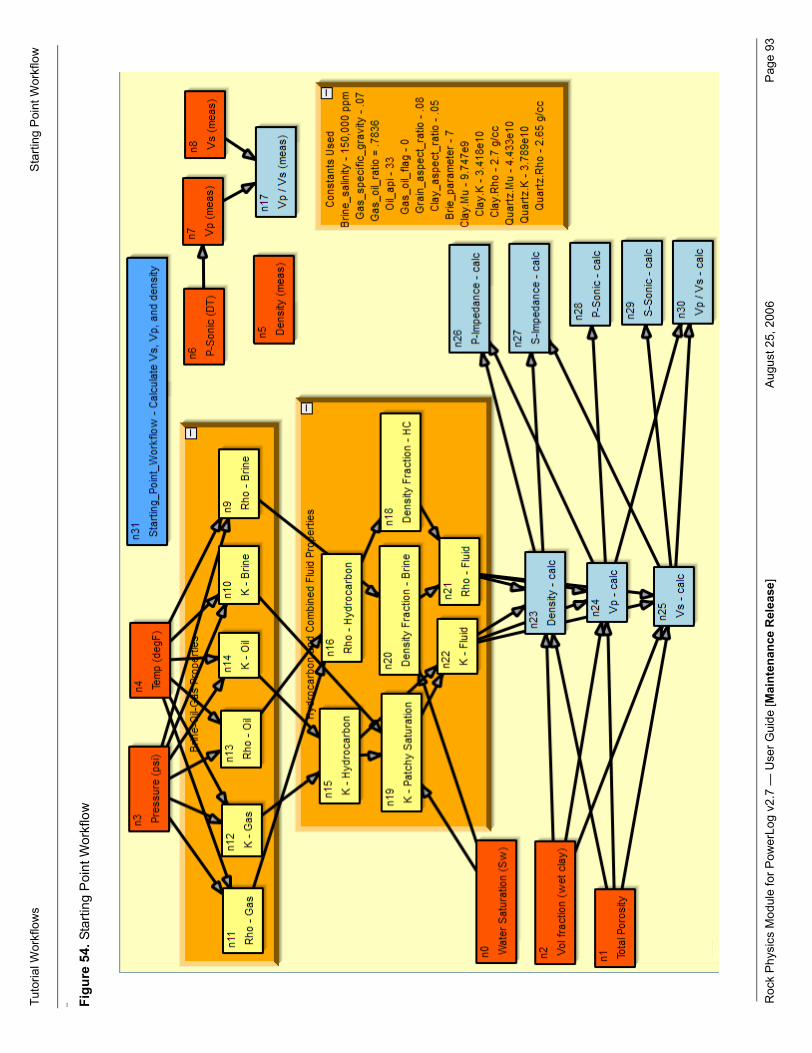
Starting Point WorkflowThe Starting Point Workflow9 helps you get oriented to organizing some of your workflow elements into various groups. In this workflow you calculate a density, Vp, and Vs curve using a number of common petrophysical curves and constants.

ObjectivesThe Starting Point Workflow:• Calculates density, acoustic velocity, and shear velocity.• Outputs PowerLog curves to use in the Curve Differences Statistics workflow to

determine a quantitative measure of the modeling effort’s success.• Illustrates how the elastic moduli from brine, oil, and gas can be calculated using

pressure, temperature, and salinity information.• Shows how to use conditional logic functions to interchange gas and oil properties

when computing the final hydrocarbon properties.• Illustrates simple usage of MixVelocity functions using simple constants for modu-

lus constants and clay velocities.• Calculates the fluid bulk modulus using Brie’s formula (Dvorkin at al. 1999 [12]) for

patchy saturation.• Describes and documents named constants to create an easy to use workflow.

Table 8. Example workflow color scheme

Workflow Element ColorColor SpecificationRed: xxx, Green: yyy, Blue: zzz

Workspace (background) Red: 255, Green: 255, Blue: 192

PowerLog input curves (nodes) Red: 255, Green: 85, Blue: 0

Computation nodes Red: 255, Green: 255, Blue: 127

Groups (background) Red: 255, Green: 170, Blue: 0

Output results (nodes) Red: 173, Green: 216, Blue: 230

Labels - workflow and constants Red: 85, Green: 170, Blue: 255

Connections Black Red: 0, Green: 0, Blue: 0

9. Many thanks to Mark Sams of Fugro-Jason for developing the initial draft of this workflow.



Jaso

n Ge

oscie

nce W

orkb

ench

7.1

Computed resultsThese PowerLog output curves are created when the entire workflow is calculated.

StrategiesThe key approach to solving this problem involves:• Using the downhole temperature, pressure information, and named constants with

the Fluid/Rock Physics for Brine, Oil, and Gas functions (BrineRho, BrineK, GasRho, GasK, LiveOilRho and LIveOilK).

• Use a conditional logic named constant Gas_oil_flag (oil=0, gas=1) to select one set of properties and designate these properties as the HC or hydrocarbon component.

• Specifying a set of clay velocity, density, and modulus constants, along with the clay pore aspect ratio to serve as inputs to the MixVelocity functions.

• Combine the brine and hydrocarbon fluid properties, with the clay properties, and use the Volume of wet clay curve as the fractional volume to run each of the MixVelocity functions (MixVelocityRho, MixVelocityVp, and MixVelocityVs).

PowerLog input curvesThese PowerLog input curves are used to calculate the brine, gas, and oil properties. The water saturation curve is used in the Brie’s patchy saturation formula (Brie et al. 1995 [6]) and to compute the density fraction of brine and hydrocarbons. The total porosity and Vclay curves are inputs to the MixVelocity functions.

Table 9. Starting Point Workflow - output curves

Node Curve Name

Type - Units Description

n17 VpVsmeas any none Measured Vp/Vs ratio, calculated from Vp and Vs measured curves

n23 rhocalc density g/cc Calculated bulk density

n24 Pvelcalc p_velocity ft/sec Calculated acoustic velocity

n25 Svelcalc s_velocity ft/sec Calculated shear velocity

n26 Zpcalc any none Calculated acoustic impedance

n27 Zscalc any none Calculated shear impedance

n28 DTpcalc p_sonic µsec/ft. Calculated acoustic sonic

n29 DTscalc s_sonic µsec/ft. Calculated shear sonic

n30 VpVscalc any none Vp / Vs velocity ratio



Jaso

n Ge

oscie

nce W

orkb

ench

7.1

Hint For your well, you may need to modify the curve names or replace them with a convenient curve alias name. The curve names in the previous table are from the tutorial Starting_Point_Workflow project.

Named Constants and Mineral PropertiesThis table displays the named constants, clay properties, grain/clay pore aspect ratios, and the conditional logic switch for gas and oil.

Table 10. Starting Point Workflow - input curves

Node Curve Name Type and Units Description

n0 SW SW none Water saturation

n1 PHIT porosity none Total porosity

n2 VCL any none Volume of Wet Clay

n3 PRES pressure psi Pressure of formation

n4 T temperature degF Downhole temperature

n5 RHOC any none Bulk density - measured

n6 DT p_sonic µsec/ft. P-sonic measured

n7 VP p_velocity ft/sec Vp measured

n8 VS s_velocity ft/sec Vs measured

Table 11. Starting Point Workflow - named constants and rock/fluid properties

Name Value Units Used in these workflow nodes

Brine_salinity 150000 ppm n9, n10—concentration

Gas_specific_gravity .07 none n11, n12, n13, n14—spec-grav

Gas_oil_ratio 44/5.615 none n13, n14—dimensionless Rs

Oil_api 33 api n13, n14—oil density

Gas_oil_flag 0 - Gasotherwise Oil

none n15, n16—select which hydrocarbon to use in the fluid computations

Clay_Vs 6233.6 ft/sec Compute µclay and Kclay

Clay_Vp 13714 ft/sec Compute µclay and Kclay

Grain_aspect_ratio .08 none n23, n24, n25—nonclay (Quartz) pore aspect ratio

Clay_aspect_ratio .05 none n23, n24, n25—Clay pore aspect ratio

Brie_parameter 7 none n19—patchy saturation computation

Clay.Mu 9.747e9 N/m2 n23, n24, n25—clay shear modulus= MuFromVel (Vs-clay, ρclay)



Jaso

n Ge

oscie

nce W

orkb

ench

7.1

Key workflow functions and formulasThe major expressions used in these workflow nodes are:• n9—ρbrine = BrineRho10(Pressurecurve, Temperaturecurve, Brine_Salinity)• n10—Kbrine = BrineK( Pressurecurve, Temperaturecurve, Brine_Salinity)• n11—ρgas = GasRho( Pressurecurve, Temperaturecurve, Gas_specific_gravity, Bat-

zle&Wang)• n12—Kgas = GasK( Pressurecurve, Temperaturecurve, Gas_specific_gravity, Bat-

zle&Wang)• n13—ρoil = LiveOilRho( Pressurecurve, Temperaturecurve, Oil_api, Gas_oil_ratio,

Gas_specific_gravity, blank, Batzle&Wang)

• n14—Koil = LiveOilK( Pressurecurve, Temperaturecurve, Oil_api, Gas_oil_ratio, Gas_specific_gravity, blank, Batzle&Wang)

• n15—KHC = ConditionalExpression( Gas_oil_flag, ==, 0, Kgas , Koil ) 11

• n16—ρHC= ConditionalExpression( Gas_oil_flag, ==, 0, ρgas, ρoil )• n17—Vp/Vsmeas = VPcurve / VScurve• n18—Density FractionHC= ( 1 - Gas_spec_gravity ) * ρHC• n19—Kpatchy = ( Kbrine - KHC ) * SWcurve ** Brie_parameter• n20—Density Fractionbrine= SWcurve * ρbrine• n21—ρfluid = ( Density Fractionbrine + Density FractionHC )• n22—Kfluid = ( Kpatchy + KHC )

Hint All three MixVelocity functions (MixVelocityRho, MixVelocityVp, and MixVelocityVs) take the same input constants and PowerLog curve names shown.

• n23— rhocalc = ρcalculated = MixVelocityRho ( PHITcurve , VCLcurve, Quartz.K, Clay.K, Quartz.Mu, Clay.Mu, Quartz.Rho, Clay.Rho, Grain_aspect_ratio, Clay_aspect_ratio, blank, blank, blank, blank, blank, blank, blank, Kfluid, ρfluid, XuWhiteApprox)

• n24— Pvelcalc = Vp_calculated = MixVelocityVp ( PHITcurve , VCLcurve, Quartz.K, Clay.K, Quartz.Mu, Clay.Mu, Quartz.Rho, Clay.Rho, Grain_aspect_ratio, Clay_aspect_ratio, blank, blank, blank, blank, blank, blank, blank, Kfluid, ρfluid, XuWhiteApprox)

Clay.K 3.418e10 N/m2 n23, n24, n25—clay bulk modulus= KFromVel (Vp-clay, Vs-clay, ρclay)

Clay_rho 2.7 g/cc n23, n24, n25—clay density

Quartz.Mu 4.433e10 N/m2 n23, n24, n25—quartz shear modulus

Quartz.K 3.789e10 N/m2 n23, n24, n25—quartz bulk modulus

Quartz.Rho 2.65 g/cc n23, n24, n25—quartz density

10.Name of the RPM rock physics function used for this node. All other nodes use mathematical functions.11.HC - Denotes hydrocarbon (oil or gas) selected with the ConditionalExpression RPM function for KHC and ρHC.

Table 11. Starting Point Workflow - named constants and rock/fluid properties (Continued)


Rock Physics Module for PowerLog v2.7 — User Guide [Maintenance Release] August 25, 2006 2


Jaso

n Ge

oscie

nce W

orkb

ench

7.1

• n25— Svelcalc = Vs_calculated = MixVelocityVs ( PHITcurve , VCLcurve, Quartz.K, Clay.K, Quartz.Mu, Clay.Mu, Quartz.Rho, Clay.Rho, Grain_aspect_ratio, Clay_aspect_ratio, blank, blank, blank, blank, blank, blank, blank, Kfluid, ρfluid, XuWhiteApprox)

• n26— Zpcalc = Zp_calculated = Vp_calculated * ρcalculated • n27— Zscalc = Zs_calculated = Vs_calculated * ρcalculated • n28— DTpcalc = ∆tp_calculated = 1000000. / Vp_calculated • n29— DTscalc = ∆ts_calculated = 1000000. / Vs_calculated• n30— VpVscalc = Vp/Vs_calculated = Vp_calculated / Vs_calculated

Roc

k P

hysi

cs M

odul

e fo

r Pow

erLo

g v2

.7 —

Use

rGui

de [M

aint

enan

ce R

elea

se]

Aug

ust 2

5, 2

006

Pag

e 93

Tuto

rial W

orkf

low

sS

tarti

ng P

oint

Wor

kflo

w

xxx Fi

gure

54.S

tarti

ng P

oint

Wor

kflo

w


Tutorial Workflows Curve Differences Statistics

Jaso

n Ge

oscie

nce W

orkb

ench

7.1

Curve Differences StatisticsThe Curve Differences Statistics workflow helps you to understand how accurately any calculated curve from a rock physics model workflow approximates the equivalent measured petrophysical log. A correlation value ≥ 0.8 suggests a strong correlation, while a value ≤ 0.5 suggests a weak correlation. You can use this workflow to assess the calculated results of the Starting Point Workflow against the measured well curves:• Density (ρ)• Vp (acoustic velocity)• Shear velocity (Vs)• Vp / Vs (acoustic / shear) velocity ratio

ObjectivesThe Curve Differences Statistics workflow:• Provides information about the accuracy of a rock physics model curve calculation.• Illustrates a workflow building block that can be used interchangeably with any set

of measured and calculated curves• Identifies if the measured and calculated (modeled) curves are strongly correlated,

suggesting that the model approximates the measured response.• Computes a quality control value in the form of the averaged RMS difference per-

centage between the calculated and measured curves. This value can be com-pared with other workflow calculations to see if the model error is decreasing or increasing due to parameter or model variations.

• Computes a bias function. A significant average bias function suggests there are unaccounted factors not described by the model.

Computed resultsThe Curve Differences Statistics workflow yields these results for each measured and calculated curves:• Error function curve (n2)—curve stored in PowerLog that can be plotted beside

the calculated and measured curves. Node n2 is where you change the name of the output error function curve.

• RMS Difference Percentage (n7)—A value that describes the average difference between the calculated and measured curves. This value is the computed as:n7—RMS Difference Percentage = 100 * ∆RMS / meanmeas, that is, the root-mean square of the curve difference, normalized by the mean of the measured curve

• Correlation Coefficient value (n3)—A value describing the amount of linear correlation between the measured and calculated curve. A correlation value ≥ 0.8 suggests a strong correlation, while a value ≤ 0.5 suggests a weak correlation.

• Average Bias Percentage (n10)—A value equal to the average deviation between the measured and calculated curve.

StrategiesThe computations in the Curve Differences Statistics workflow are a straightforward usage of the Correlation, Mean, Sum, and Rms RPM statistical functions.


Tutorial Workflows Curve Differences Statistics

Jaso

n Ge

oscie

nce W

orkb

ench

7.1

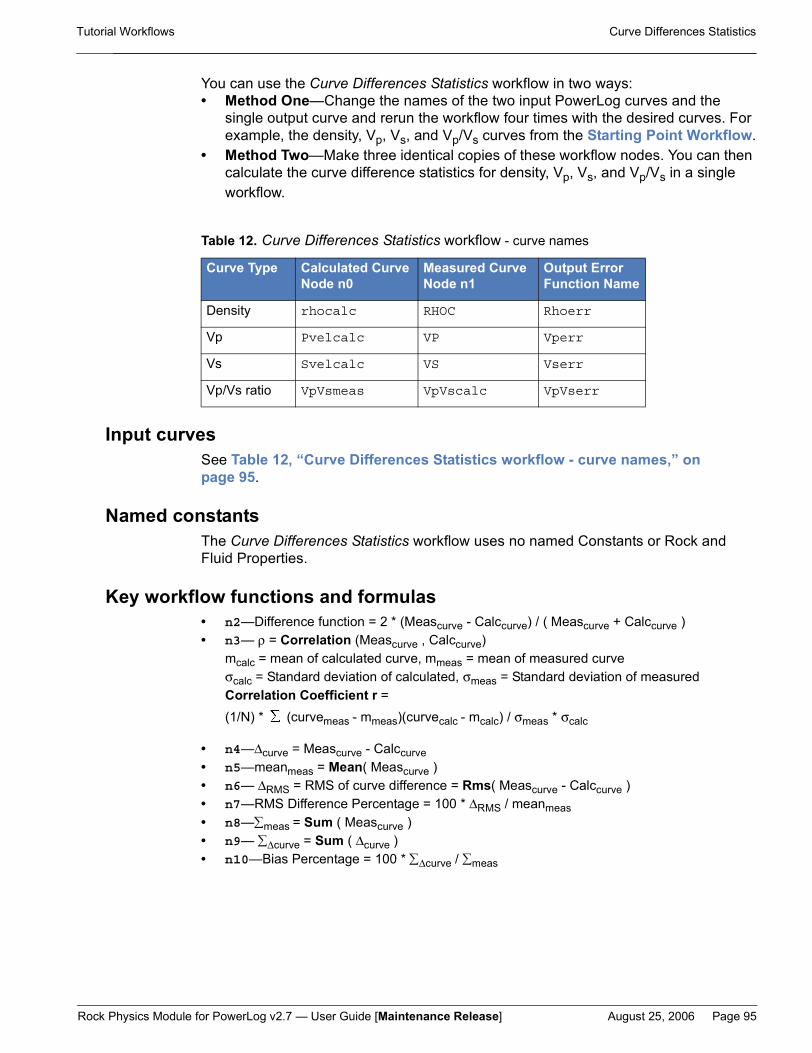
You can use the Curve Differences Statistics workflow in two ways:• Method One—Change the names of the two input PowerLog curves and the

single output curve and rerun the workflow four times with the desired curves. For example, the density, Vp, Vs, and Vp/Vs curves from the Starting Point Workflow.

• Method Two—Make three identical copies of these workflow nodes. You can then calculate the curve difference statistics for density, Vp, Vs, and Vp/Vs in a single workflow.

Input curvesSee Table 12, “Curve Differences Statistics workflow - curve names,” on page 95.

Named constantsThe Curve Differences Statistics workflow uses no named Constants or Rock and Fluid Properties.

Key workflow functions and formulas• n2—Difference function = 2 * (Meascurve - Calccurve) / ( Meascurve + Calccurve )• n3— ρ = Correlation (Meascurve , Calccurve)

mcalc = mean of calculated curve, mmeas = mean of measured curveσcalc = Standard deviation of calculated, σmeas = Standard deviation of measured Correlation Coefficient r = (1/N) * (curvemeas - mmeas)(curvecalc - mcalc) / σmeas * σcalc

• n4—∆curve = Meascurve - Calccurve• n5—meanmeas = Mean( Meascurve )• n6— ∆RMS = RMS of curve difference = Rms( Meascurve - Calccurve )• n7—RMS Difference Percentage = 100 * ∆RMS / meanmeas • n8—∑meas = Sum ( Meascurve )• n9— ∑∆curve = Sum ( ∆curve )• n10—Bias Percentage = 100 * ∑∆curve / ∑meas

Table 12. Curve Differences Statistics workflow - curve names

Curve Type Calculated CurveNode n0

Measured CurveNode n1

Output Error Function Name

Density rhocalc RHOC Rhoerr

Vp Pvelcalc VP Vperr

Vs Svelcalc VS Vserr

Vp/Vs ratio VpVsmeas VpVscalc VpVserr

Roc

k P

hysi

cs M

odul

e fo

r Pow

erLo

g v2

.7 —

Use

rGui

de [M

aint

enan

ce R

elea

se]

Aug

ust 2

5, 2

006

Pag

e 96

Tuto

rial W

orkf

low

sC

urve

Diff

eren

ces

Sta

tistic

s

Figu

re55

.Cur

ve D

iffer

ence

s St

atis

tics

wor

kflo

w


Tutorial Workflows SimpleExpression formulas and logic

Jaso

n Ge

oscie

nce W

orkb

ench

7.1

SimpleExpression formulas and logicThis workflow demonstrates some of the computational formulas and sophisticated logic possible with the SimpleExpression function in RPM for PowerLog.

ObjectivesThe SimpleExpression formulas and logic workflow demonstrates how to:• Control the computation sequence using parentheses• Implement multiple decision logic two ways to determine a:

– curve that is limited between an minimum and a maximum value– lithology coding– fluid substitution value

• Implement a rock physics formula not found in RPM– Brie’s patchy saturation formula– λρ lambda-density product and µρ mu-density product– Poisson’s ratio12

– Young’s modulus

Named ConstantsThis table displays the named constants, for the SimpleExpression formulas and logic workflow.

12.The Poisson function does perform this calculation.

Table 13. SimpleExpression formulas and logic workflow - named constants


Sonic_min 90 µsec/ft. n3, n5—minimum sonic transit time

Sonic_max 100 µsec/ft. n3, n5—maximum sonic transit time

Previous_value 2 none n6, used in n11 and n10—previous lithology log value determination

Min_clay_volume .4 none n7, n11—minimum clay volume for calcareous shale

Min_coal_volume .1 none n8, n11—minimum coal volume for calcareous shale

Min_quartz_dominates .5 none n9, n11—maximum quartz volume for calcareous shale

Calcareous_shale 1 none n10, n11—value representing cal-careous shale for lithology log

Vol_clay_max .2 none n12, n17—maximum clay volume permitted for fluid substitution

Phi_effective_min .05 none n14, n17—minimum effective poros-ity required for fluid substitution



Jaso

n Ge

oscie

nce W

orkb

ench

7.1

Key workflow functions and formulasThe SimpleExpression formulas and logic workflow uses a few nodes and the SimpleExpression function to demonstrate each concept listed in the Objectives.

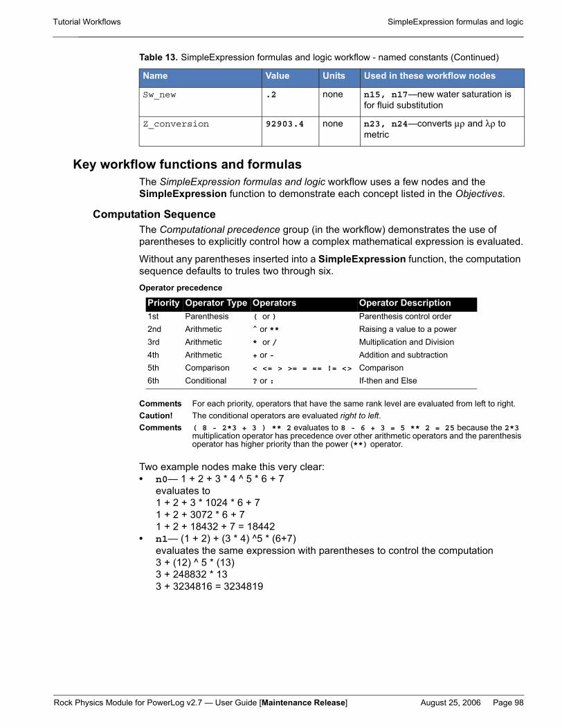
Computation SequenceThe Computational precedence group (in the workflow) demonstrates the use of parentheses to explicitly control how a complex mathematical expression is evaluated.

Without any parentheses inserted into a SimpleExpression function, the computation sequence defaults to trules two through six.Operator precedence

Comments For each priority, operators that have the same rank level are evaluated from left to right.Caution! The conditional operators are evaluated right to left.Comments ( 8 - 2*3 + 3 ) ** 2 evaluates to 8 - 6 + 3 = 5 ** 2 = 25 because the 2*3

multiplication operator has precedence over other arithmetic operators and the parenthesis operator has higher priority than the power (**) operator.

Two example nodes make this very clear:• n0— 1 + 2 + 3 * 4 ^ 5 * 6 + 7

evaluates to1 + 2 + 3 * 1024 * 6 + 71 + 2 + 3072 * 6 + 71 + 2 + 18432 + 7 = 18442

• n1— (1 + 2) + (3 * 4) ^5 * (6+7) evaluates the same expression with parentheses to control the computation3 + (12) ^ 5 * (13)3 + 248832 * 133 + 3234816 = 3234819

Sw_new .2 none n15, n17—new water saturation is for fluid substitution

Z_conversion 92903.4 none n23, n24—converts µρ and λρ to metric

Priority Operator Type Operators Operator Description1st Parenthesis ( or ) Parenthesis control order2nd Arithmetic ^ or ** Raising a value to a power3rd Arithmetic * or / Multiplication and Division4th Arithmetic + or - Addition and subtraction5th Comparison < <= > >= = == != <> Comparison6th Conditional ? or : If-then and Else

Table 13. SimpleExpression formulas and logic workflow - named constants (Continued)




Jaso

n Ge

oscie

nce W

orkb

ench

7.1

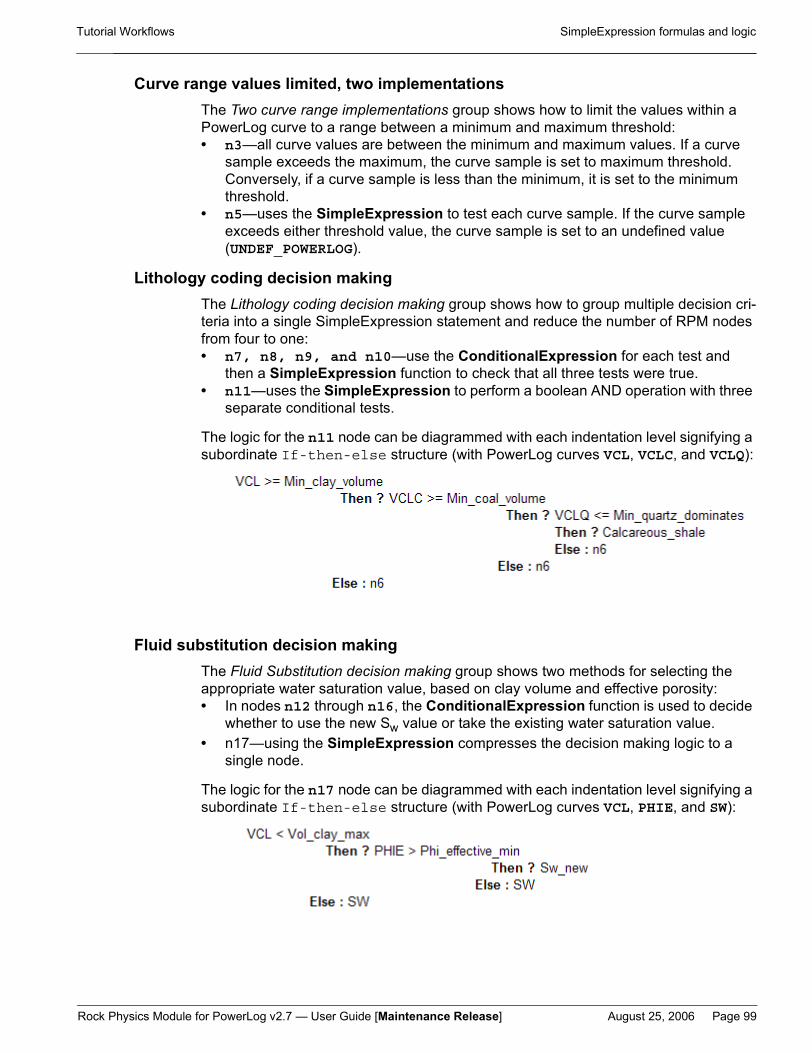
Curve range values limited, two implementationsThe Two curve range implementations group shows how to limit the values within a PowerLog curve to a range between a minimum and maximum threshold:• n3—all curve values are between the minimum and maximum values. If a curve

sample exceeds the maximum, the curve sample is set to maximum threshold. Conversely, if a curve sample is less than the minimum, it is set to the minimum threshold.

• n5—uses the SimpleExpression to test each curve sample. If the curve sample exceeds either threshold value, the curve sample is set to an undefined value (UNDEF_POWERLOG).

Lithology coding decision makingThe Lithology coding decision making group shows how to group multiple decision cri-teria into a single SimpleExpression statement and reduce the number of RPM nodes from four to one:• n7, n8, n9, and n10—use the ConditionalExpression for each test and

then a SimpleExpression function to check that all three tests were true.• n11—uses the SimpleExpression to perform a boolean AND operation with three

separate conditional tests.

The logic for the n11 node can be diagrammed with each indentation level signifying a subordinate If-then-else structure (with PowerLog curves VCL, VCLC, and VCLQ):

Fluid substitution decision makingThe Fluid Substitution decision making group shows two methods for selecting the appropriate water saturation value, based on clay volume and effective porosity:• In nodes n12 through n16, the ConditionalExpression function is used to decide

whether to use the new Sw value or take the existing water saturation value.• n17—using the SimpleExpression compresses the decision making logic to a

single node.

The logic for the n17 node can be diagrammed with each indentation level signifying a subordinate If-then-else structure (with PowerLog curves VCL, PHIE, and SW):



Jaso

n Ge

oscie

nce W

orkb

ench

7.1

Rock physics formulasThe Rock Physics Formulas group implements four expressions for elastic moduli:

• Poisson’s ratio (n20 and n26)— ν = (1/2) [ (Vp/Vs)2 - 2] / (Vp/Vs)2 - 1 ) • λρ and µρ (n18, n19, n23, and n24)—

µρ = Vs2ρ2 * Z_Conversion, where Z_Conversion converts to metric units

λρ = Vp2ρ2 * Z_Conversion - 2*µρ

• Youngs Modulus (n21, n22, n25, and n27)— E = ρ*Vs

2 * [ (3*Vp2 - 4*Vs

2) / (Vp2 - Vs

2 ) ]

Roc

k P

hysi

cs M

odul

e fo

r Pow

erLo

g v2

.7 —

Use

rGui

de [M

aint

enan

ce R

elea

se]

Aug

ust 2

5, 2

006

Pag

e 10

1

Tuto

rial W

orkf

low

sS

impl

eExp

ress

ion

form

ulas

and

logi

c

xxxx

x Figu

re56

.Sim

pleE

xpre

ssio

n fo

rmul

as a

nd lo

gic

wor

kflo

w


Tutorial Workflows RP Properties for AVO Checks

Jaso

n Ge

oscie

nce W

orkb

ench

7.1

RP Properties for AVO ChecksThe RP Properties for AVO Checks workflow uses density, acoustic log, and shear velocity log to calculate elastic constants that are useful in checking direct hydrocarbon indicators. Goodway et al. [15] suggested that Lamé’s elastic parameters λ and µ, and their products with density, can be useful tools in AVO analysis.

In particular, λ*ρ is very sensitive to fluids, while µ*ρ has little variation within the reservoir zone. Smith and Gidlow [35] plotted Castagna and Smith’s [9] set of 25 world-wide measurements of P- and S-wave velocities and densities. Cross-plot domain representations of 25 shale/brine sand, shale/gas sand, and gas sand/brine- sand sets using Vs vs. Vp crossplots and µρ vs. λρ crossplots clearly showed the distinction between gas-sands and non-pay lithologies,

ObjectivesThe RP Properties for AVO Checks workflow:• Provides standard calculations of Vp and Vs velocities along with the acoustic

impedance I = Vpρ and shear impedance J = Vsρ. for:– Corrected acoustic ∆tp, shear ∆ts, and density logs– Identify wet sand acoustic ∆tp, shear ∆ts, and density interval– Raw acoustic ∆tp, shear ∆ts, and density logs

• Calculate effective porosity based on measured volume of clay• Calculate elastic moduli for bulk modulus (K), shear modulus (µ), Young’s

modulus (E), Poisson’s ratio (ν), shear modulus*density product (µρ), and Lamé’s constant*density product (λρ).

• Illustrate how to restrict the range of a petrophysical curve values so that Vp/Vs ratios are reasonable. Curve values that exceed the range for ∆ts result in Vp/Vs points that are undefined (UNDEF).

Computed resultsThese PowerLog output curves are created when the entire workflow is calculated.

Table 14. RP Properties for AVO Checks Workflow - output curves

Node Curve Name

Type and Units Description

n12 Vp p_velocity ft/sec Acoustic velocity - corrected

n13 Vs s_velocity ft/sec Shear velocity - corrected

n14 VpVscor any none Vp/Vs ratio, calculated from Vp and Vs corrected

n16 Zp_cor any none Acoustic impedance - corrected

n17 Zs_cor any none Shear impedance - corrected

n21 Lithfrac any none Lithology fraction

n22 Phi_eff any none Effective porosity

n8 Vp_wet p_velocity ft/sec Acoustic velocity - wet sand



Jaso

n Ge

oscie

nce W

orkb

ench

7.1

PowerLog input curvesThese PowerLog input curves are used to calculate the acoustic velocity and impedance, as well as the shear velocity and impedance. This workflow can use the corrected sonic and density logs, plus the raw logs for its Vp/Vs ratio calculations. The corrected density and velocities are used to calculate the three elastic moduli (Young’s, bulk, and shear), plus Poisson’s ratio and two AVO-related hydrocarbon indicators.

Hint For your well, you may need to modify the curve names or replace them with a convenient curve alias name. The curve names in the this table are from the tutorial RP_Properties_for_AVO_Checks_Workflow project.

n9 Vs_wet s_velocity ft/sec Shear velocity - wet sand

n10 Zp_wet any none Acoustic impedance - wet sand

n11 Zs_wet any none Shear impedance - wet sand

n18 Poisson any none Poisson’s ratio

n19 MuRho any none µρ hydrocarbon indicator

n20 LameRho any none λρ hydrocarbon indicator

n34 E_cor any N/m2 Young’s modulus - corrected

n35 K_cor bulk_modulusN/m2

Bulk modulus - corrected

n36 Mu_cor shear_modulusN/m2

Shear modulus - corrected

n39 VpVs_raw any none Vp/Vs ratios from raw curves, where Vs was limited to specific range defined by the named constants: Min_shear_tdel to Max_shear_tdel.Vs values outside this range yield an undefined value for the corresponding Vp/Vs ratio.

Table 15. RP Properties for AVO Checks Workflow - input curves


n0 DTC p_sonic µsec/ft. P-sonic corrected

n1 RHOC density g/cc Density corrected

n2 DTS s_sonic µsec/ft. S-sonic corrected

n3 PHIT porosity none Total porosity

n4 VCL any none Volume of Wet Clay

Table 14. RP Properties for AVO Checks Workflow - output curves (Continued)

Node Curve Name




Jaso

n Ge

oscie

nce W

orkb

ench

7.1

Named ConstantsThe RP Properties for AVO Checks workflow uses these named constants:• Convert_Impedance_to_Metric—92903.4• Max_shear_tdel—300 µsec/ft.• Min_shear_tdel—100 µsec/ft.

Key workflow functions and formulas• n8, n9, n12, n13, n26, n28—these workflow nodes implement the simple

division to convert a sonic log to the corresponding velocity values using the for-mula: Velocityx_curve = 1000000 / ∆tx, where x = p (acoustic), x = s (shear)

• n10, n11, n16, n17, n29, n30—these workflow nodes calculate the acousticor shear impedance, using the product of the velocity and density curves:Zx_curve = Velocityx_curve * ρcurve, where x = p (acoustic), x = s (shear)

• n18—Poisson’s ratio computed using ν = (1/2) [ (Vp/Vs)2 - 2] / (Vp/Vs)2 - 1 ) • n19—MuRho product = µρ = Vs

2ρ2 * Convert_Impedance_to_Metric• nn20—LambdaRho product = λρ = Vp

2ρ2 * Convert_Impedance_to_Metric - 2*µρ • n22—ϕeff_curve = (1 - Vclaycurve) * PHITcurve

• n34—Young’s modulus E = ρ*Vs2 * [ (3*Vp

2 - 4*Vs2) / (Vp

2 - Vs2 ) ]

• n35—Bulk modulus K = KFromVel ( Vp, Vs, ρ )• n36—Shear modulus µ = MuFromVel ( Vs, ρ )• n39—Vp/Vs measured = Vp/Vs , if Min_shear_tdel ≤ ∆ts ≤ Max_shear_tdel

otherwise Vp/Vs measured = UNDEF_POWERLOG

n5 DTC p_sonic µsec/ft. P-sonic (wet)

n6 RHOC density g/cc Density (wet)

n7 DTS s_sonic µsec/ft. S-sonic (wet)

n23 DT_raw p_sonic µsec/ft. P-sonic (raw) - uncorrected

n25 RHOCraw density g/cc Density (raw) - uncorrected

n24 DTS_raw s_sonic µsec/ft. S-sonic (raw) - uncorrected

Table 15. RP Properties for AVO Checks Workflow - input curves (Continued)


Roc

k P

hysi

cs M

odul

e fo

r Pow

erLo

g v2

.7 —

Use

rGui

de [M

aint

enan

ce R

elea

se]

Aug

ust 2

5, 2

006

Pag

e 10

5

Tuto

rial W

orkf

low

sR

P P

rope

rties

for A

VO

Che

cks

Figu

re57

.RP

Pro

perti

es fo

r AV

O C

heck

s w

orkf

low


Tutorial Workflows Fluid properties to estimate Vs

Jaso

n Ge

oscie

nce W

orkb

ench

7.1

Fluid properties to estimate VsThe Fluid properties to estimate Vs workflow calculates the density and bulk modulus for the subsurface fluids (brine, oil, and gas) as a function of:• Pressure• Temperature• Salinity• Oil and gas gravity• Gas oil ratio

ObjectivesThe Fluid properties to estimate Vs workflow shows you:• How to use conditional logic (named constant and ConditionalExpression func-

tion) to select between a PowerLog curve and a constant as an input parameter.• Compute density and bulk modulus using the Brine, Oil, and Gas functions.• Use named constants as physical parameters and as workflow logic switches.• Select the oil or gas properties as the dominant hydrocarbon, using the

ConditionalExpression function.

Computed resultsThese PowerLog output curves are created when the entire workflow is calculated. Additionally, when a PowerLog curve is selected for use, the mean value of the calculated curves is also determined in the workflow.

Hint If you do not want to add the mean calculation nodes to your workflow, you can use the F8 (Calculate workflow) command to calculate the workflow. Once it finishes, you can place the mouse on each of the Curve Nodes in the next table. For each node, the function is shown in a tool tip and the node output curve name, mean value, and number of defined samples is displayed in the status bar. See Figure: 87, ‘Status bar”, on page 146.

Table 16. Fluid properties to estimate Vs workflow - output curves

Curve Nodes

Curve Name

MeanNodes


n7 Salinity n12 salinity ppm Salinity input

n13 D_brine n21 density g/cc Density of brine

n14 K_brine n22 modulus N/m2 Bulk modulus of brine

n15 Den_gas n23 density g/cc Density of gas

n16 K_gas n24 modulus N/m2 Bulk modulus of gas

n17 Den_oil n25 density g/cc Density of oil

n18 K_oil n26 modulus N/m2 Bulk modulus of oil

n19 Den_hydr n27 density g/cc Selected hydrocarbon density

n20 K_hydr n28 modulus N/m2 Selected hydrocarbon bulk modulus



Jaso

n Ge

oscie

nce W

orkb

ench

7.1

PowerLog input curvesThese six PowerLog input curves are used to compute the density and bulk modulus of the fluid properties.

Hint For your well, you may need to modify the curve names or replace them with a convenient curve alias name. The curve names in the this table are from the tutorial Fluid_properties_to_estimate_Vs project.

Named constantsThe named constants for the Fluid properties to estimate Vs workflow consists of two groups; one set for physical fluid properties and the other to control the workflow computations.

Table 17. Fluid properties to estimate Vs workflow - input curves




n2 Sal salinity ppm Brine salinity

n3 API oil api Oil gravity

n4 SPEC any api Gas specific gravity

n5 GOR any none Gas oil ratio

Table 18. Fluid properties to estimate Vs workflow - named constants

Constant Name Value Units Used in nodes

Salinity_brine 72000 ppm n7

Oil_gravity 43 api n8

Gas_specific_gravity .65 none n10

Gas_oil_ratio 15000 none n11

Constant Name used asconditional logic flag

Value Units Used in nodes

Salinity_LogOrConstant 1 = Log, else constant none n7

Oil_grav_LogOrConstant 1 = Log, else constant none n8

Gas_grav_LogOrConstant 1 = Log, else constant none n10

GasOilRatio_LogOrConstant 1 = Log, else constant none n11

Hydrocarbon_gasoil_select 0 = Gas, otherwise oil none n19, n20



Jaso

n Ge

oscie

nce W

orkb

ench

7.1

Key workflow functions and formulasMost of the functions used in the Fluid properties to estimate Vs workflow, are the Brine, Oil, and Gas functions (see online help from each of the workflow nodes).

The ConditionalExpression function:• Selects between a PowerLog curve and a constant value for salinity, oil gravity,

gas specific gravity, and the gas-oil ratio inputs.• Selects between the computed oil and gas constants (hydrocarbon density and

bulk modulus) for this workflow calculation.

The Brine, Oil, and Gas functions used in this workflow are:• n13—ρbrine = BrineRho (Pressure, Temp, salinitiy)• n14—Κbrine = BrineK (Pressure, Temp, salinitiy)• n15—ρgas = GasRho (Pressure, Temp, spec, Batzle&Wang)• n16—Κgas = GasK (Pressure, Temp, spec, Batzle&Wang)• n17—ρoil = LiveOilRho (Pressure, Temp, oil_api, Rs, spec, blank,

Batzle&Wang)• n18—Κoil = DeadOilK (Pressure, Temp, oil_api, Batzle&Wang)

The general form for the Conditional logic that selects a curve or constant is:if (curvename_LogOrConstant == 1) then Curve, else Constant

The form for the Conditional logic that selects gas or oil is:if (Hydrocarbon_gasoil_select == 0) then Gas, else Oil

Roc

k P

hysi

cs M

odul

e fo

r Pow

erLo

g v2

.7 —

Use

rGui

de [M

aint

enan

ce R

elea

se]

Aug

ust 2

5, 2

006

Pag

e 10

9

Tuto

rial W

orkf

low

sFl

uid

prop

ertie

s to

est

imat

e V

s

Figu

re58

.Flu

id p

rope

rties

to e

stim

ate

Vs

wor

kflo

w


Tutorial Workflows Lithology log construction

Jaso

n Ge

oscie

nce W

orkb

ench

7.1

Lithology log constructionPetrophysicists construct lithology logs using many combinations of measured logs to infer geology and potential production zones. This RPM for PowerLog workflow uses six input PowerLog curves to construct a lithology coding log.

ObjectivesThe Lithology log construction workflow:• Illustrates how a lithology log can be constructed by replacing petrophysical log

measurements with rock physics parameters.• Describes how to use name constants and RPM functions to define complex

logical expressions.

Computed resultsThe Lithology log construction workflow result is a single PowerLog curve (LITHTYPE, N26) with lithology coding. The values are coded in the Table 20, “Lithology log construction workflow - named constants,” on page 111.• 0 = shale (default)• 1 = calcareous shale• 2 = limestone• 3 = coal• 4 = sand• 5 = gas sand

PowerLog input curvesHint For your well, you may need to modify the curve names or replace them with a

convenient curve alias name. The curve names in the this table are from the tutorial Lithology_log_construction_workflow project.

Named constantsThe Lithology log construction workflow uses two sets of named constants; one to specify the decision making constants and another to implement the lithology coding.

Table 19. Lithology log construction workflow - input curves


n0 VCLC any none Volume of calcite relative to total volume (correct shale velocity)

n1 VCOA any none Volume of coal relative to total volume

n2 VCL any none Volume of clay relative to total volume

n3 VQUA any none Volume of quartz relative to total volume

n4 PIGE any none Effective porosity minus irreducible water

n5 Sw Sw none Water saturation


Tutorial Workflows Lithology log construction

Jaso

n Ge

oscie

nce W

orkb

ench

7.1

Throughout the conditional logic nodes in the Lithology log construction workflow, these values are used. If you want to extend these indicators, create additional named constants similar to the ones in the previous table.

Key workflow functions and formulasWithin these workflow nodes you can use either the ConditionalExpression or SimpleExpression functions to implement the decision logic. When multiple conditions must be combined (nodes n17, n18, and n19), set the output of each separate condition equal to 1 and test to see that all conditions (node n20) are true:

• n12— If (all curve samples not UNDEF) then LITHTYPE = Shale_lith, else UNDEF• n15— If (Volcalcite ≥ Min_calcite_volume) then LITHTYPE = Limestone_lith• n16— If (Volcoal ≥ Min_coal_dominates) then LITHTYPE = Coal_lith• n17, n18, n19, n20— If (Volclay ≥ Min_clay_volume ) AND

( Volcoal ≥ Min_coal_volume ) AND ( Volquartz ≤ Min_clay_volume ) then LITHTYPE = Calcareous_shale_lith

• n21, n22, n23— If ( Volquartz ≥ Min_quartz_volume ) AND( PIGE ≥ Min_porosity_effective) then LITHTYPE = Sand_lith

• n24, n25, n26— If ( LITHTYPE = Sand_lith ) AND (Rw ≤ Max_Sw_gassand)then LITHTYPE = GasSand_lith

Table 20. Lithology log construction workflow - named constants

Lithology coding constants Value Units Used in nodes

Shale_lith 0 n/a none

Calcareous_shale_lith 1 n/a n20

Limestone_lith 2 n/a n15

Coal_lith 3 n/a n16

Sand_lith 4 n/a n23

GasSand_lith 5 n/a n26

Conditional logic constants Value Units Used in nodes

Min_calcite_volume .45 none n15

Min_coal_dominates .5 none n16

Min_clay_volume .4 none n17

Min_coal_volume .1 none n18

Min_quartz_dominates .5 none n19

Min_quartz_volume .45 none n21

Min_porosity_effective .08 none n22

Max_Sw_gassand .7 none n25

Roc

k P

hysi

cs M

odul

e fo

r Pow

erLo

g v2

.7 —

Use

rGui

de [M

aint

enan

ce R

elea

se]

Aug

ust 2

5, 2

006

Pag

e 11

2

Tuto

rial W

orkf

low

sLi

thol

ogy

log

cons

truct

ion

Figu

re59

.Lith

olog

y lo

g co

nstru

ctio

n w

orkf

low


Tutorial Workflows Gassmann fluid-substitution to predict seismic response

Jaso

n Ge

oscie

nce W

orkb

ench

7.1

Gassmann fluid-substitution to predict seismic responseThe Gassmann fluid-substitution to predict seismic response workflow performs a hydrocarbon fluid substitution for the original brine in reservoir rocks so that the resulting velocity change can predict the seismic response of oil or gas in a reservoir. The Sw measured in the logs describes the original fluid composition.

Fluid substitution criteriaThe workflow dynamically determines whether to perform the fluid substitution:• For rocks with good porosity and low clay content (reservoir rocks), you perform a

fluid substitution that reduces Sw to a lower level, thus increasing the hydrocarbon content.

• For rocks that do not meet the porosity and clay content criteria (non-reservoir rocks), the original Sw log is retained and no fluid substitution takes place.

The cutoff for wet clay content (Vclay) in good reservoirs is found in named constant, Vol_clay_max. The Vclay maximum is initially set at 0.20, but can be adjusted.The cutoff for effective porosity (PHIE) in good reservoirs is found in the named constant Phi_effective_max. You can change the value (effective porosity maximum = 0.05) by editing the named constant.

Thus rocks with Vclay < 0.2 and PHIEcurve >0.05 are considered reservoir rocks and fluid substitution is performed in these rocks. Sw in these rocks becomes 0.20, instead of the initial value in the Sw curve. The replacement value for Sw is set in the named constant Sw_new, and can be adjusted.

Fluid substitution overviewPowerLog Pressure and Temperature logs are used in the Brine, Gas, and Oil Properties group to compute the properties of the individual fluids in the borehole.

The properties of the original combined fluid are computed in the Combined Fluid Properties (OLD) group. The Water Saturation (Sw_old) node inputs the Sw curve from PowerLog, which determines the Sw prior to any fluid replacement. Brie’s formula for patchy saturation is used to compute the bulk modulus and density of the combined fluid in the Brie’s Formula (OLD) group. The empirical Brie parameter (set to one) can be adjusted as the named constant Brie_oldfluid_parameter.

Next, the we compute the elastic parameters for a new fluid (brine in the original fluid replaced by hydrocarbons), but only in rocks with good porosity and low clay content. The selection of rocks with good porosity and low clay content (good reservoir rocks) takes place in the Fluid Substitution Criteria Check group. PowerLog for effective porosity, bulk density, (wet) clay content, and velocities are found in the Gassmann Inputs group.

The new Sw (the replacement value in reservoir rocks, the old value in all other rocks) is computed in the SwFluid Sub node in the Combined Fluid Properties (NEW) group. The bulk modulus and density of the replacement fluid are computed in this group just like the Combined Fluid Properties (OLD) group. Brie’s patchy saturation formula in the Brie’s Formula (NEW) group is used again. The Brie parameter is again set to one in the named constant Brie_newfluid_parameter.



Jaso

n Ge

oscie

nce W

orkb

ench

7.1

The bulk modulus for the solid matrix is computed from a weighting of the K for clay (in the Kclay Fraction node) and the K for quartz (in the Kquartz Fraction node). Bulk modulus values for the minerals can be changed by using the Rock and FLuid Properties dialog.

Results from workflowFinally, the Gassmann substitution, using the fluid parameters for the substituted fluid (which differ only in the reservoir rocks) is computed in the Gassmann FluidSub node. The rock density with the new fluid, P-sonic travel time, acoustic velocity (GassmannFull function), and impedance are calculated in the final workflow nodes.

Data consistency issuesCaution! There is sometimes a data-consistency issue with GassmannFull function in the

Gassmann FluidSub node if input logs for the original rock (before the fluid substitu-tion) are not sufficiently consistent with the relationship: K = Vp

2 * ρ – 4/3*µ,where µ = Vs

2 * ρ and Vp, Vs, and ρ are calculated from log petrophysical analysis.

Bulk modulus K is independent of the input parameters for the densities and bulk and shear moduli of the mineral and fluid constituents of the rock-physics model. But K and the constituents of the model are used together in the Gassmann formula to calculate the bulk modulus of the rock with the initial fluid removed (the dry frame), and with a replacement fluid.

Problems in the Gassmann calculation can occur if the rock-physics model chosen is not consistent with the ρ, Vp, and Vs data from the logs (in other words, if the model just is not a good match for the rocks in the well), or if the log ρ and velocity data are not internally consistent. If such inconsistencies are present, the GassmannFull function displays error messages and stops before producing an output curve.

These parameter conditions produce error messages:• K ≤ 0, produces the error “Input bulk modulus illegal”• Kdry (the bulk modulus of the rock frame without fluid), calculated from

Gassmann’s formula using K ≤ 0, or greater than K for the mineral members, produces the error “Calculated empty frame modulus illegal”.

ObjectivesThe Gassmann fluid-substitution to predict seismic response workflow:• Dynamically tests Vcl to see if the clay content is too high and ensures the effective

porosity exceeds a minimum level before performing a fluid substitution at each log depth.

• Uses Brie’s formula to compute the bulk modulus (K) and density (ρ) of the combined fluid for the brine in reservoir rocks. It independently use’s Brie’s formula for patchy saturation again to compute K and ρ for the oil or gas replacement.

Computed resultsThe Gassmann fluid-substitution to predict seismic response workflow results permit you to predict appropriate seismic velocities and impedance.



Jaso

n Ge

oscie

nce W

orkb

ench

7.1

StrategiesTo perform the fluid substitution effectively:• Elastic properties (bulk modulus and density) of the original fluid, composed of

brine (plus some gas or oil) are computed.• A Gas/Oil conditional logic named constant group to chooses gas or oil (oil may

contain gas) in the original fluid.• Elastic parameters for a new fluid (much of the brine in the original fluid is replaced

by hydrocarbons) are computed for rocks with good porosity and low clay content.• The cutoffs for Vclay and ϕeff porosity are defined; Vclay cutoff is initially = 0.20 and

the initial value for the PHIE cutoff = 0.05.• The new Sw (the replacement value in reservoir rocks, the old value in all other

rocks) is computed in the SwFluid Sub node.• The bulk modulus for the solid matrix is computed from a weighting of the K for

clay.• The Gassmann substitution, using the fluid parameters for the substituted fluid

(which differ in the reservoir rocks), is done in the Gassmann FluidSub node.

PowerLog input curvesThese PowerLog input curves are used to calculate the brine, gas, and oil properties. The water saturation curve is used in the Brie’s patchy saturation formula and to compute the density fraction of brine and hydrocarbons. The total porosity and Vclay curves are inputs to the fluid substitution and Kmineral groups.

Hint For your well, you may need to modify the curve names or replace them with a convenient curve alias. The curve names in the previous table are from the tutorial Gassmann_fluid_substitution_predict_seismic_response project.

Table 21. Gassmann fluid-substitution to predict seismic response workflow - output curves

Curve Nodes

Curve Name


n30 SW_NEW Sw none Water saturation curve - taking into account the new fluid substitution

n36 Den_fsub density g/cc Bulk density with replacement fluid

n37 Vp_fsub P-velocity ft/sec Velocity for hydrocarbon substitution

n38 Sonic_fs p_sonic µsec/ft. ∆tp for hydrocarbon substitution

n39 Zp_fsub any none Acoustic impedance

Table 22. Gassmann fluid-substitution to predict seismic response workflow - input curves




n3 SW Sw none Water saturation



Jaso

n Ge

oscie

nce W

orkb

ench

7.1

Named Constants and Mineral PropertiesThis table displays the named constants, clay and quartz bulk modulus, and the conditional logic switch (Gas_oil_selection) for gas and oil.

n4 PHIE porosity none Effective Porosity

n5 VCL any none Volume fraction of clay relative to total volume

n6 RHOC any none Bulk density - measured

n7 Vpcalcr p_velocity ft/sec Vp log

n8 Vscalcr s_velocity ft/sec Vs log

Table 23. Gassmann fluid-substitution to predict seismic response workflow - named constant and rock/fluid properties


Brine_salinity 150000 ppm n13, n14—concentration in ppm

Gas_specific_grav .07 none n9, n10, n11, n12— Gas spec-grav

Gas_oil_ratio 44 none GOR (Gas Oil Ratio)

GOR_conversion 5.615 none Factor compute dimensionless Rs

Oil_API 33 api n11, n12—oil density

Gas_oil_selection 0 - Gaselse Oil

none n18, n19—select which hydrocarbon to use in the fluid computations

Brie_oldfluid_parameter

1 none n24—Brie exponent for old fluid patchy saturation computation

Brie_newfluid_parameter

1 none n34—Brie exponent for new fluid patchy saturation computation

Phi_effective_min .05 none n22—minimum porosity needed for fluid substitution

Vol_clay_max 7 none nxx, nxx—maximum clay volume allowed for fluid substitution

Rs_dimensionless 7.83615 none n11, n12—GOR dimensionless value

Sw_new .2 none n21—Sw replacement value

Clay.K 2.091e10 N/m2 n15—clay bulk modulus

Quartz.K 3.789e10 N/m2 n16—quartz bulk modulus

Table 22. Gassmann fluid-substitution to predict seismic response workflow - input curves




Jaso

n Ge

oscie

nce W

orkb

ench

7.1

Key workflow functions and formulas• n09—ρgas = GasRho13 (Pressurecurve, Temperaturecurve, Gas_specific_grav,

Batzle&Wang)• n10—Kgas = GasK (Pressurecurve, Temperaturecurve, Gas_specific_grav, Batzle&Wang)• n11—ρoil = LiveOilRho (Pressurecurve, Temperaturecurve, Oil_API, Rs_dimensionless,

Gas_specific_grav, blank, Batzle&Wang)

• n12—Koil = LiveOilK (Pressurecurve, Temperaturecurve, Oil_API, Rs_dimensionless, Gas_specific_grav, blank, Batzle&Wang)

• n13—Kbrine = BrineK (Pressurecurve, Temperaturecurve, Brine_salinity)• n14—ρbrine = BrineRho (Pressurecurve, Temperaturecurve, Brine_salinity)• n15—Kclay_frac = Vcl * Clay.K• n16—Kquartz_frac = (1-Vcl) * Quartz.K• n17—Kmineral = Kclay_frac + Kquartz_frac

• n18—KHC = ConditionalExpression( Gas_oil_selection, ==, 0, Kgas , Koil ) 14

• n19—ρHC= ConditionalExpression( Gas_oil_selection, ==, 0, ρgas, ρoil )• n20—ρBrine_frac_(old) = ρbrine * SWcurve• n21—Vclay test = ConditionalExpression( Vcl_curve, <, Vol_clay_max, 1, 0 )• n22—ϕeff test = ConditionalExpression( ϕeff _curve, >, Phi_effective_min, Vclay test,

0 )• n23—ρHC_frac_(old) = ρHC * (1 - SWcurve)• n24—KBrie_(old)= ( Kbrine - KHC ) * SWcurve ** Brie_oldfluid_parameter• n26—No Fluid Sub = (1 - ϕeff test)* SWcurve [use Sw old]• n27—Fluid Sub = (ϕeff test)*Sw_new [use Sw new]• n28—ρfluid_(old) = ρHC_frac(old) + ρBrine_frac_(old)• n29—Kfluid_(old) = KHC + KBrie_(old)• n30—SW_NEWcurve = Sw_FluidSub = Fluid Sub + No Fluid Sub• n31—ρBrine_Frac_(new) = Sw_FluidSub * ρBrine• n32—ρHC_Frac_(new) = (1 - Sw_FluidSub) * ρBrine• n33—ρFluid_(new) = ρBrine_Frac_(new) + ρHC_Frac_(new) • n34—KBrie_(new) = ( Kbrine - KHC ) * SWcurve ** Brie_newfluid_parameter• n35—KFluid_(new) = KBrie_(new) + KHC • n36—Den_fsubcurve = ρFsub = RHOCcurve + ϕeff * ( ρFluid_(new) - ρFluid_(old) )• n37—Vp_fsubcurve = GassmannFull (Vpcurve, Vscurve, RHOCcurve, ϕeff, KFluid_(new),

ρFluid_(new), Kmineral, KFluid_(old), ρFluid_(old) )• n38—Sonic_fscurve = Psonic - Fsub = 1000000. / Vp_fsubcurve • n39—Zp_fsubcurve = Vp_fsubcurve * Den_fsubcurve

13.Name of the RPM rock physics function used for this node.14.HC - Denotes hydrocarbon (oil or gas) selected with the ConditionalExpression RPM function for KHC and ρHC.

Roc

k P

hysi

cs M

odul

e fo

r Pow

erLo

g v2

.7 —

Use

rGui

de [M

aint

enan

ce R

elea

se]

Aug

ust 2

5, 2

006

Pag

e 11

8

Tuto

rial W

orkf

low

sG

assm

ann

fluid

-sub

stitu

tion

to p

redi

ct s

eism

ic re

spon

se

Figu

re60

.Gas

sman

n flu

id-s

ubst

itutio

n to

pre

dict

sei

smic

resp

onse

rpm tutorial workflows for petrophysical log...

Documents