rrt*-smart: a rapid convergence implementation of...

International Journal of Advanced Robotic Systems

RRT*-SMART: A Rapid Convergence Implementation of RRT* Regular Paper

Jauwairia Nasir1,2, Fahad Islam1,2, Usman Malik1, Yasar Ayaz1, Osman Hasan2, Mushtaq Khan1 and Mannan Saeed Muhammad1,3,* 1 Robotics & Intelligent Systems Engineering (RISE) Lab, Department of Robotics and Artificial Intelligence, School of Mechanical & Manufacturing Engineering (SMME), National University of Sciences and Technology (NUST), Islamabad, Pakistan 2 Department of Electrical Engineering, School of Electrical Engineering & Computer Sciences (SEECS), National University of Sciences and Technology (NUST), Islamabad, Pakistan 3 Department of Electronic Engineering, College of Engineering, Hanyang University, Seoul, South Korea * Corresponding author E-mail: [email protected] Received 30 May 2012; Accepted 3 Jun 2013 DOI: 10.5772/56718 © 2013 Nasir et al.; licensee InTech. This is an open access article distributed under the terms of the Creative Commons Attribution License (http://creativecommons.org/licenses/by/3.0), which permits unrestricted use, distribution, and reproduction in any medium, provided the original work is properly cited.

Abstract Many sampling based algorithms have been introduced recently. Among them Rapidly Exploring Random Tree (RRT) is one of the quickest and the most efficient obstacle free path finding algorithm. Although it ensures probabilistic completeness, it cannot guarantee finding the most optimal path. Rapidly Exploring Random Tree Star (RRT*), a recently proposed extension of RRT, claims to achieve convergence towards the optimal solution thus ensuring asymptotic optimality along with probabilistic completeness. However, it has been proven to take an infinite time to do so and with a slow convergence rate. In this paper an extension of RRT*, called as RRT*-Smart, has been prposed to overcome the limitaions of RRT*. The goal of the proposecd method is to accelerate the rate of convergence, in order to reach an optimum or near optimum solution at a much faster rate, thus reducing the execution time. The novel approach of the proposed algorithm makes use of two new techniques in RRT*--Path Optimization and Intelligent Sampling. Simulation results presented in various obstacle cluttered environments along with statistical and mathematical

analysis confirm the efficiency of the proposed RRT*-Smart algorithm. Keywords Biasing Radius, Path Optimization, Biasing Ratio

1. Introduction

Motion Planning is a domain which involves finding a feasible trajectory that connects the starting point to the goal point while avoiding collision with the obstacles. The geometry of Robot and the obstacles is defined in a 2D or 3D configuration workspace and the motion is represented by a path in the configuration space. Motion planning has a lot of applications in various fields including autonomy, automation, architectural designs, AI for video games, digital character animations, molecular biology and robotic surgery. The field of Motion Planning and Navigation has gained immense popularity and importance in the recent years due to the fact that current trends in robotics research for both

1Jauwairia Nasir, Fahad Islam, Usman Malik, Yasar Ayaz, Osman Hasan, Mushtaq Khan and Mannan Saeed Muhammad: RRT*-SMART: A Rapid Convergence Implementation of RRT*

www.intechopen.com

ARTICLE

www.intechopen.com Int. j. adv. robot. syst., 2013, Vol. 10, 299:2013

industrial and domestic needs are focused towards intelligent automation. In the last four decades, many path planning algorithms, including geometric, grid-based, potential field, neural networks, genetic and sampling based algorithms, have been proposed for various static and dynamic environments. Each of these algorithms has its own advantages and shortcomings in finding the most efficient path planning solution in terms of space and time complexity and path optimization [1-6]. Sampling based algorithms are among the latest and most popular path planning algorithms. As compared to other probabilistically complete algorithms, they are computationally less complex, and have the ability to find solutions without using explicit information about the obstacles in the configuration space. They rely on a collision checking module and build a roadmap of feasible trajectories made by connecting together a set of points sampled from the obstacle-free space. An extensive comparative study and analysis of a number of sampling based techniques has been presented by various researchers over the years [7], [8], and [10]. Rapidly Exploring Random Tree (RRT) [9], is one of the quickest algorithms in finding the first path but it does not ensure asymptotic optimality [10]. To improve the efficiency of the RRT algorithm, various methods have been presented including potential function planner [11], density avoided sampling [12] including variations of such planners as well [13-17]. However, the major breakthrough came with the development of RRT* in 2010 [10]. Rapidly Exploring Random Tree Star (RRT*) is one of the recent sampling based algorithms which was also presented as an extension to RRT. Its major advantage over other algorithms is that it finds an initial path very quickly and then later keeps on optimizing it as the number of samples increases. Thus, apart from probabilistic completeness it ensures asymptotic optimality [10], unlike the predecessor sampling based algorithms like RRT [10], [13], Probabalistic Road Map (PRM) [14] and RRTConnect [13]. A few recent sampling based algorithms are also asymptotically optimal like PRM* [14] and RRG [10], yet RRT* has the advantage over these planners in terms of both time complexity and space complexity as explained by Keraman and Frazolli in [10]. Although RRT* claims to reach an optimal solution, it never reaches that optimality in finite time [10]. Also, the rate of convergence is slow. This manuscript addresses these issues by introducing RRT*-Smart, which instead of employing purely random space exploration, performs an informed exploration of search space. It makes use of the first path found by RRT* as an intelligent guess to help in exploring the configuration space. Moreover, it uses intelligent sampling to give an optimum or near optimum path at a very fast rate of convergence and reduced execution time. The solution obtained by RRT*-Smart also

facilitates the robot to track the trajectory as it is straighter and with less way points. Thus, it gives a more efficient path planning solution as compared to RRT*. The algorithm proposed, in this manuscript, demonstrantes these distinguishing features through experimental results and performance analysis. The remainder of the paper is organized as follows. In Section 2, RRT* is discussed. RRT*-Smart is presented in Section 3. Sections 4 cover results and performance analysis. Section 5 explains the optimization parameters. Section 6 concludes the paper and highlights future research avenues.

2. RRT* Algorithm

This section briefly introduce motion planning using the RRT* algorithm to build the background for understanding RRT*-Smart. RRT* is an incremental sampling based algorithm which finds an initial path very quickly. The path is later optimized as the execution takes place [10], [20]. Let X define the configuration space in which Xobs is the obstacle region, Xfree = X / Xobstacle is the obstacle-free region and Xgoal is the goal region. RRT* works to find out an input u: [0:T] ϵ U that yields a feasible path x(t) ϵ Xfree that starts from x(0) = x-initial to x(T)= goal following the system constraints. While finding this solution, RRT* maintains a tree Ƭ= (V, E) of vertices V sampled from the obstacle-free state space Xfree and edges E that connect these vertices together. This algorithm makes use of a set of procedures which are explained as below : Sampling: It randomly samples a state zrand ϵ Xfree from the obstacle-free configuration space. Distance: This function returns the cost of the path between two states assuming the region between them is obstacle free. The cost is in terms of Euclidean distance. Nearest Neighbor: The function Nearest(Ƭ, zrand) returns the nearest node from Ƭ=(V, E) to zrand in terms of the cost determined by the distance function. Steer: The function Steer (zrand, znearest) solves for a control input u[0,T] that drives the system from x(0)=zrand to x(T)=znearest along the path x: [0,T] → X giving znew at a distance ∆q from znearest towards zrand where ∆q is the incremental distance. Collision Check: The function Obstaclefree(x) determines whether a path x:[0,T] lies in the obstacle-free region Xfree for all t=0 to t=T. Near-by Vertices: The function Near(Ƭ, zrand, n) returns the nearby neighboring nodes that lie in a ball of volume (β

2 Int. j. adv. robot. syst., 2013, Vol. 10, 299:2013 www.intechopen.com

(logn/n)) around zrand, where β is a constant that depends on the planner. Insert node: The function Insertnode(zparent, znew, Ƭ) adds a node znew to V in the tree Ƭ =(V, E) and connects it to an already existing node zparent as its parent, and adds this edge to E. A cost is assigned to znew which is equal to the cost of its parent plus the Euclidean cost returned by the Distance function between znew and its parent zparent. Rewire: The function Rewire(Ƭ, Znear, zmin, znew) checks if the cost to the nodes in Znear is less through znew as compared to their older costs. If it is for a particular node, its parent zparent is changed to znew.

Pseudocode describing RRT* is shown in Algorithm 1. 1 Ƭ ← InitializeTree(); 2 Ƭ ← InsertNode(Ø, zinit, Ƭ); 3 for i=0 to i=N do 4 zrand ← Sample(i); 5 znearest ← Nearest(Ƭ, zrand); 6 (xnew, unew, Tnew) ← Steer (znearest, zrand); 7 if Obstaclefree(xnew) then 8 Znear ← Near(Ƭ, znew, |V|); 9 zmin ← Chooseparent (Znear, znearest, znew, xnew); 10 Ƭ ← InsertNode(zmin, znew, Ƭ); 11 Ƭ ← Rewire (Ƭ, Znear, zmin, znew); 12 return Ƭ

Algorithm 1. Ƭ = (V, E) ← RRT*(zinit)

At first, a sample zrand is placed randomly in the configuration space Xfree. Then, the nearest node znearest to zrand is checked for in the entire configuration space. A node znew is placed at a distance ∆q from the nearest node znearest in the line of direction of zrand. Then, the trajectory path xnew is checked if it is free of obstacles. If the trajectory is obstacle free then a ball of radius β(logn/n) around znew is checked for near nodes Znear. Among this set of nodes, the node that gives the least cost from the starting point to znew through itself is selected as the parent of znew. Once the parent is selected, rewiring takes place. The costs of all the nodes inside this ball around znew is calculated through znew. If this cost is less than the previous cost for any node then that particular node is disconnected from its old parent and is connected to znew as its parent. RRT* is a landmark sampling based algorithm to approach an optimal solution ensuring asymptotic optimality, apart from probabilistic completeness, as opposed to its predecessor RRT (and its various other improved versions). Although it tends to approach an optimal solution but it has been proven mathematically that it reaches the said solution in infinite time [10]. To overcome these limitations, a rapid convergence version of RRT* known as RRT*-Smart is proposed in this paper, which moves towards an optimal solution at a significantly faster rate.

3. RRT*-Smart Algorithm

This section describes the RRT*-Smart algorithm and the two proposed key concepts --Intelligent Sampling and Path Optimization. Initially, RRT*-Smart randomly searches the state space as RRT* does. Similarly, the first path is found just like the RRT* would try to find a path by random sampling in the configuration space. Once this first path is found, it then optimizes it by interconnecting the directly visible nodes. This optimized path yields biasing points for intelligent sampling. At these biasing points, sampling takes place at regular intervals, which are governed by a constant b that in turn depends upon the biaisng ratio explained in Section 6. This process is continued, as the algorithm progresses and the path is optimized continuously. Whenever, a shorter path is found, the biasing shifts towards the new path. This process is outlined in Algorithm 2. 1 Ƭ ← InitializeTree(); 2 Ƭ ← InsertNode(Ø, zinit, Ƭ); 3 for i=0 to i=N do 4 if i=n+b, n+2b, n+3b…. then 5 zrand ← Sample(i, zbeacons); 6 else 7 zrand ← Sample(i); 8 znearest ← Nearest(Ƭ, zrand); 9 (xnew, unew, Tnew) ← Steer (znearest, zrand); 10 if Obstaclefree(xnew) then 11 Znear ← Near(Ƭ, znew, |V|); 12 zmin ← Chooseparent (Znear, znearest, znew, xnew); 13 Ƭ ← InsertNode(zmin, znew, Ƭ); 14 Ƭ ← Rewire (Ƭ, Znear, zmin, znew); 15 if InitialPathFound then 16 n ← i; 17 (Ƭ, directcost) ← PathOptimization(Ƭ, zinit, zgoal); 18 if (directcostnew < directcostold) 19 zbeacons ← PathOptimization(Ƭ, zinit, zgoal); 20 return Ƭ

Algorithm 2. Ƭ = (V,E) ← RRT*Smart(zinit)

The steps 1 to 3 and 7 to 14 execute in the same way as the corresponding ones in RRT*. Once the initial path is found, (i.e., in step 15) the function InitialPathFound returns the iteration number n at which this path is found. This n is then used to inform the algorithm when to start the biased sampling. This biased sampling then starts with an interval time defined by the constant b. The function (Ƭ, directcost) ← PathOptimization(Ƭ, zinit, zgoal) determines an optimized path by directly connecting the nodes in the path that are visible to each other and returns its cost (step 17). In steps 18 and 19 beacons (the nodes which form the basis for intelligent sampling) are being formed from the function zbeacons ← PathOptimization(Ƭ, zinit, zgoal), only if the new cost is less than the old cost. Otherwise, the old beacons keep on biasing the tree. In steps 4-5, zrand ← Sample (i, zbeacons), samples are being spawned at the beacons within a ball of radius Rbeacons centered at zbeacons. After the initial beacons


www.intechopen.com

are found, intelligent sampling takes place with a certain percentage; i.e., after every few samples that are placed in the normal way as for RRT* (steps 7 to 9), one sample is spawned in the vicinity of the beacons.

3.1 Path Optimization

Once RRT* gives an initial path, the nodes in the path x: [zinit, zgoal] → X that are visible to each other are directly connected. An iterative process starts from zgoal and moves towards zinit checking for direct connections with successive parents of each node until the collision free condition fails. By the end of this process, no more directly connectable nodes are present. Hence the path is optimized based on the concept of the Triangular Inequality as illustrated in Fig. 1. According to the Triangular Inequality, c is always less than the sum of a and b, and hence always gives a shorter path. The proposed path optimization is elaborated in Algorithm 3, where, zvc is a visibilty check node, which is used for notation in the psuedocode.

Figure 1. Path Optimization based on Triangular Inequality.

1 while (! visible nodes) 2 zvc = zgoal ; 3 while ( ! zinit) 4 if Obstaclefree (zvc, zvc-parent-to-parent) 5 zvc-parent = zvc-parent-to-parent ; 6 zvc = zvc-parent ; Algorithm 3. (Ƭ, directcost) ← PathOptimization(Ƭ, zinit, zgoal)

The number of nodes present in this path are thus reduced, as compared to the original path found by RRT*. These nodes are termed as Beacons (zbeacons), which form the basis for intelligent sampling. Every time a new RRT* path with a shorter cost is found, it is optimized by the path optimization technique to give a relatively better path. The cost of this optimized path is compared with the cost of the previous optimized path. If the cost is better, then the nodes that are present in this path are selected as beacons zbeacons, for intelligent sampling. At each visibility check between two nodes, the collision free check is required. For this purpose, an interpolation technique is utilized in the proposed method, which works by constructing every point on the line (by

connecting all the nodes together), while making sure that the newly added points lie in the free configuration space. This method of visibility check does not need explicit information about obstacles as required in other collision checking methods, [21]. Hence, the proposed method of interpolation for collision free checking is independent of the shape of the obstacles and is computationally less expensive.

3.2 Intelligent Sampling

The idea behind intelligent sampling is to approach optimality by generating the nodes as close as possible to the obstacle vertices following the underlining idea of visibility graph technique. However, the visibility graph techniques require complex environmental modeling and explicit information about obstacles, [2]. Furthermore the basic visibility graph method may not reach a solution in environments containing obstacles with complex geometries (concave, polygonal, circular etc). Some solutions in this regard have been presented like Reduced Visibility Graphs [22], which improve the efficiency of visibility graphs. Whereas, Generalised Visibility Graphs [22], are an extension of the basic technique that form paths around intricate complex geometries. However, in doing so, the computational complexity for Generalised Visibility Graphs is increased to a great extent as it find solution for all the complex gemotroies present in the configuration space. On the other hand, in sampling based RRT*-Smart, the path is optimized only along the periphery of those obtscales which lie along the optimum path or the intermediate paths. Once the initial path has been found, intelligent sampling starts with a certain number of samples being directly spawned (steps 4 and 5 of Algorithm 2) in a ball of radius Rbeacons centered at zbeacons. The sampling is biased towards these beacons because they provide useful clues regarding the position of obstacle vertices (or periphery in the case of circular obstacles). Therefore, these beacons need to be surrounded by maximum nodes to optimize the path at these turns. This feature forces the proposed algorithm to reach the optimal solution in less number of iterations, as compared to RRT*, as later demonstrated in the experimental results section of this paper. As the algorithm iterates an optimized path is calculated, when ever a new RRT* path is found.. The cost of this new optimized path is compared with the previous optimized path. If the cost is smaller, new beacons, zbeacons, are generated resulting in the formation of new biasing points. These newly formed beacons are closer to the vertices. This process continues until the required iterations are completed. Although the obstacles are not being explicitly defined by keeping the beneficial property of sampling based algorithms intact; the proposed algorithm finds a way to


spawn the tree nearer to the vertices by using intelligent guessing and biasing beacons, which eventually leads towards an optimal/near-optimal path x:[zinit,zgoal] →optimal X. This path also has a very few number of samples which are shown in Section 5. Hence, the RRT*-Smart algorithm works to provide a much better solution at a faster rate of convergence. The proposed algorithm also finds a simpler path for the mobile robots to follow in any kind of environment due to the less number of waypoints.

Figure 2. (a) First Path given by RRT* at n=650. (b) An optimized path (in blue) is shown after the Path Optimization technique is applied on the path shown in (a). (c) shows clustered samples as a result of biasing towards the beacons (in green) at n=2500; (d) shows the optimum path at n=4200

Fig. 2 demonstrates the effectiveness and working of the RRT*-Smart algorithm. An initial path is found in Fig. 2(a) at n=650. In Fig. 2(b), path optimization yields an optimized path, as shown in blue. The green dots are the beacons that are formed for this initial path. After n=2500, clustered samples are formed around the beacons, as demonstrated in Fig. 2(c). Finally, after an iterative process, an optimized path is found for this obstacle scenario at n=4200. The space and time complexity for RRT* are given by O(n) and O(nlogn), respectively [10]. Mathematical analysis of RRT*-Smart shows that the space and time complexity is the same as that of RRT* but the value of n is significantly reduced in case of RRT*-Smart. Thus, O(n) and O(nlogn) for RRT*Smart yields much better performance. However, as the performance improves and the biasing ratio increases, the randomness in the exploration of the tree decreases as a number of nodes are now used to optimize the path in a particular region. Therefore, there is a tradeoff between intelligent sampling and the space exploration rate.

4. Results and Performance Comparison

This section demonstrates the results for RRT*-Smart in four seperate environments, each with different obstacle scenario. The statistical and analytical comparison between RRT* and RRT*-Smart is also presented in this section, along with a t-student test for testing equality of the means for the two methods. In the figures, the hollow red box represents the goal region; the solid red blocks represent the obstacles while the trajectory is depicted by a black line. The algorithm provides an optimal/near-optimal solution in the circular, local minima and cluttered environment. It can be observed that the path optimization and the intelligent sampling techniques, that this algorithm employs, is independent of the obstacle shape, as highlighted in the previous section. It not only optimizes the path for obstacles with straight edges but also for those with rounded peripheries, as illustrated in Fig. 3(a).

Figure 3. RRT*-Smart in different obstacle Environments with constant biasing ratio

The number of beacons that are being used to optimize the path in each obstacle environment may be different. In case of rounded obstacles as in Fig. 3(a), the number of beacons may be significantly greater than in cases where the obstacles are with straight edges. This is due to the reason that now more number of nodes are required to cover the circular periphery of the obstacle to provide the most optimum path possible.

4.1 Statistical Analysis

An experimental comparison between RRT*-Smart and RRT* by analyzing their performance from various perspectives is presented in this section. At first, the results of the two algorithms in Fig. 4 are used to illustrate their comparative differences.


www.intechopen.com

Figure 4. A comparison of RRT* and RRT*-Smart using simulation results at 800, 1200 and 4200 iterations.

It is clear from the Fig. 4(d) that RRT*-Smart uses the RRT* path with a cost of 630.18 at the iteration number n =800 shown in Fig. 4(a) and finds a more optimal path with a cost of 584.02, as shown in Fig. 4(d), with an equal number of iterations using the path optimization technique. Utilizing intelligent sampling and further path optimization, the cost in Fig. 4(e) has further reduced to 557.478 at n=1200 while RRT* converging with its original rate manages to reach a cost of 624.95 with an equal number of iterations, as shown in Fig. 4(b). Finally, RRT*- Smart gives an optimal/near-optimal solution at n=4200 with a cost of 540.12 as shown in Fig. 4(f). With the same number of iterations, RRT* converges to a path with a cost of 574.009, Fig. 4(c). The efficiency in terms of path cost is evident from this comparison. A statistical comparison between the two algorithms using graphical results for the experiment is shown in Fig. 5. The figure clearly demonstrates the convergence pattern of the costs of RRT* and RRT*-Smart. It can be seen that RRT*-Smart not only has a much faster rate of convergence but also approaches the optimum cost after finite iterations whereas RRT* is still in the process of reaching an optimal solution with relatively slower ratof convergence. In Fig. 6, iterations are plotted against different fixed costs. It can be observed that for approaching the same cost, as the algorithms iterate, towards finding an optimal solution the number of iterations for RRT* is far greater than RRT*-Smart. The cost of 540 is achieved by the latter algorithm at 4200 iterations whereas RRT* fails to achieve this cost even at very large number of iterations, as shown by the same graph. Fig. 7 shows the path cost versus time comparison for the implementation of the

two algorithms. It is observed that RRT* takes significantly greater time as compared to RRT*-Smart in reaching the same cost. These results have been obtained using a 2.1 GHz Intel corei3 processor with a 4GB RAM.

Figure 5. Costs are plotted against iterations showing the rate of convergence of both RRT* and RRT*-Smart.

Figure 6. Iterations are plotted against different fixed costs.

15000

2260029500∞

800 900 1400 4200

0

10000

20000

30000

40000

563 557 555 540

Num

ber o

f ite

ratio

ns

Costs

RRT*

RRT*Smart


Figure 7. Time comparison against fixed costs. Constant b is taken as 2 for RRT*-Smart.

Fig. 8 highlights the running time ratio of RRT* to RRT*-Smart. The graph shows that the ratio is always greater than 1 for the implementation of both algorithms, proving the time efficiency of RRT*-Smart over RRT*.

Figure 8. Running Time Ratio of RRT* over RRT*-Smart is plotted against iterations. Constant b is taken as 2 for RRT*-Smart.

Figure 9. Costs of path in fifty different environments for 2500 iterations with dynamic biasing ratio scheme.

Fig. 9 demonstrates the behavior of RRT* and RRT*-Smart in fifty different obstacle environments. For each

environment, the cost is plotted for a fixed number of iterations n. It can be seen that the graph of RRT*-Smart consistently stays below the graph of RRT*, showing that in all these environments the path costs found by RRT*-Smart remains less than the path costs of RRT*, hence proving the efficiency of RRT*-Smart. Analyzing the performance comparison results, it can be concluded that RRT*-Smart is more efficient than RRT* not only with respect to path optimization but also in terms of computational time.

Comparative Statistical Analysis using t-Student test:

The two algorithms are compared in three different environments; including a maze, a narrow passage and a cluttered environment (with increasing number of obstacles), each solved for atleast 5 times. Fig.10 shows the results for one particular instance out of the five experiments performed in a Maze and a narrow passage environment, for both RRT*-Smart and RRT*. In Fig.10 (a and c), the red hollow box represents the goal region while in Fig.10(b and d), S and G denote the starting point and the goal position respectively. Similarly, Fig.11 compares the two algorithms in the cluttered environment, again for one particular instance, with increasing number of obstacles. In each figure, the obstacles are represented in red color, the goal region is shown by a red box and the trajectory is represented in black. The results are summmarized in Table 1. followed by a statistical analysis of t-Student test for testing equality of the means of the two methods. This statistical test called t-Student test is often used by the researchers and scientists to assess whether two groups significantly differ from one another. We performed an unpaired t-test between the two sets of samples, one for RRT*-Smart and the other for RRT*. Each set consists of 5 values of path costs calculated after solving that particular environment for 5 times considering the stochastic nature of the methods. The cost in each case contributes to the data, that is used to perform this test. The minimum, maximum, average, standard deviation values and the t-value for each experiment (along with the reference tabulated value z for 95 % confidence level) at 8 degress of freedom are presented in Table I. Comparing the value of t with the tabulated values of 2.31 (p=0.05) to 5.04 (p=0.001), it is observed that the value of t of the proposed scheme is greater in each case as compared to the other methods. Thus, according to the principles t-test theory, the difference between the means is very significant and so clearly RRT*-Smart provides significantly improved costs as compared to RRT* for the same number of iterations.

266368

636 ∞

8 9 11 51

0

200

400

600

800

563 557 555 540

Tim

e (s

ecs)

Costs

RRT*

RRT*Smart


www.intechopen.com

Figure 10. A comparison of RRT* and RRT*-Smart in environments with maze and narrow path.

Environment Algorithm Iterations Minimum Maximum Average Standard Deviation t value z Maze

(Fig. 10 a,c) RRT*-Smart 2000 664 672 668 2.97 28.8 2.31

RRT* 720 727 722 2.95 Narrow Passage

(Fig. 10 b,d) RRT*-Smart 2500 597 607 602 4.34 15.2 2.31

RRT* 631 637 633 2.28 Cluttered with 5 obstacles

(Fig. 11 a,e) RRT*-Smart 2000 575 582 578 2.77 14.4 2.31


(Fig. 11 b,f) RRT*-Smart 2000 603 609 607 2.49 11.0 2.31


(Fig. 11 c,g) RRT*-Smart 2000 583 591 588 3.13 36.3 2.31


(Fig. 11 d,h) RRT*-Smart 2500 601 605 603 2 18.8 2.31

RRT* 631 639 635 3.29

Table 1. Statistical comparison of RRT* and RRT*-Smart using the t-student test.

Figure 11. A comparison of RRT* and RRT*-Smart using simulation results in environments with 5, 50, 100 and 200 obstacles.


4.2 Complexity Analysis

The space and time complexity of RRT* as demonstrated in [10] is given by O(n) and O(nlogn). Mathematical analysis of RRT*-Smart shows that its space and time complexity also same as of RRT, but the value of n is significantly reduced in order to achieve same optimality. Hence, the proposed method yields better performance as compared to RRT*.

Space Complexity

Space complexity of an algorithm is defined as the amount of memory that is required by an algorithm to execute. It is clear by the above discussion that RRT*-Smart requires n number of memory configurations for n number of iterations to execute. Hence showing a linear space complexity of O(n), just like RRT*.

Time Complexity

Time complexity of an algorithm is defined as the amount of time that is required by the algorithm to execute a problem of size n. The additional steps of path optimization, intelligent sampling and the collision checking method of interpolation that have been introduced in RRT*-Smart have complexities that are insignificant enough to have no effect on the complexity of the algorithm. The analysis of the T-Notation for both RRT* and RRT*-Smart, shows that for the same number of iterations the time for RRT*-Smart is significantly less as compared to RRT*.

Complexity of the Path Optimization step

Path optimization technique is applied when ever a new smaller path as compared to the previous one is found. Let us assume that the new path is found for Delta number of times. The computational complexity of this step be given by:

Delta x Direct cost

Where, Direct cost = {f x yf/2 x (Cost of each collision check)} yf is number of nodes in the RRT* path found for each iteration f. f is number of times the iterative process is repeated for each path until all the visible nodes are directly connected. The cost of a collision check is always some constant value. As the path will move towards optimization, the direct cost will reduce with time. It is interesting to note here that the upper bound of Delta depends upon the particular environment but will always be significantly less than the total number of iterations n, and would always be a finite value for reaching an optimal solution in a particular obstacle scenario. This is due to the finite

number of the path (or the paths) which lead to optimal solution, and are significantly small in comparison to n. Hence, making this term ineffective in terms of computational complexity as it is independent of the number of iterations n.

Delta <<< n

This is supported by statistical results for three different obstacle scenarios, as shown in Table II. In each of these scenarios, the algorithm is executed until the optimized path is found. Environment Optimized

Cost Iterations Required (n)

Delta Result

Circular (Fig3(a)) 237 9100 17 Delta<<nPotential(Fig3(b)) 382 7500 22 Delta<<nCluttered(Fig3(c)) 408 13000 55 Delta<<n

Table 2. A comparison of values of delta and n in three different obstacle scenarios

Complexity of Intelligent Sampling step

Let p be a constant which defines the number of times a node will be placed at a beacon. This depends on the the constant b. Greater the biasing ratio, greater will be the value of p for the same configuration space and number of iterations. So, the complexity of this time may be given by p×c where c is a constant time to place a sample.

Reduced complexity of Sample, Nearest and Steer Step

Each of these steps will now execute (n-p) times because for p times the nodes are being placed directly at the beacons zbeacons, whereas, n is equal to the total number of iterations. Though this does not effect the O-Notation in any way but explains the reduced computational complexity and one of the factors that leads to reduced execution time as demonstrated in Fig. 7. Thus, it can be concluded that the O-Notation for the time complexity of RRT*-Smart is unaffected by the additional steps. The performance of RRT*-Smart has been improved as: 1. n is significantly reduced and 2. Execution of RRT* sample step, nearest step and steer

step has been reduced by a factor p, replaced by a single step with the same computational complexity as that of RRT* sample step, and also, a path optimization step which has an insignificant contribution as Delta <<< n.

5. Algorithm Characteristics

5.1 Biasing Radius

Biasing radius is the radius of sphere within which biasing takes place around Zbeacon. The radius Rbeacon can be


www.intechopen.com

chosen according to the planner’s requirements. For a relatively larger Rbeacon in a configuration space, the path has a greater chance of moving quickly towards an optimum path, and then with continuing iterations, the convergence rate slows down. On the other hand, when the radius Rbeacon is small for the same configuration space, the convergence rate of the path towards an optimum solution will be slower, but once an optimum enough path is found, it is more certain to reach an optimized value at a faster rate. This might be seen as a tradeoff between the planning time and the navigation time. If, for example, a motion planning and navigation problem is put up which could be solved by using this algorithm, and also which is more concerned about reducing planning time rather than navigation time, then the better solution for it will be a larger radius and vice versa. However, there is a limit to increasing the radius. If, it is increased to a very large value then the algorithm’s behaviour becomes very identical to that of RRT*. For the environment shown in Fig. 2, the experimental results for various biaising radius vs the number of iterations to reach the same cost is presented in a tabulated form in Table III. As the size of radius is increased beyond a certain level, the number of iterations required to reach the optimum cost increases significantly hence approaching the trend of RRT*, as for biasing radius of 25 in the Table III . A biasing radius in the range of 10 to 15 is used for all the experiments performed in a configuration space of the same size. A good approximation is to use a biasing radius in accordance with the size of the configuration space.

Biasing Radius Number of Iterations Cost 11 4300 540 13 4600 540 15 5200 540 17 8000 540 25 40000 540

Table 3. No. Of iterations for different biaisng radius to achieve the same cost of 450 at a biaisng ratio of 2

5.2 Biaising Ratio

Biasing ratio determines the number of times a sample has been spawned directly at a beacon instead of being sampled normally. For a constant biasing ratio throughout the entire planning phase, the choice depends upon the planner. It must be noted that changing this ratio does affect the trend of reaching optimality. The effect of choosing different constant biasing ratio for the same obstacle environment is evident from the results shown in Table IV. These results have been obtained by using the environment of Fig. 3(c).

The results shown in Table IV demonstrate that for the same environment, there exists an optimized value of biasing ratio that balances the rate of biasing and exploration to give the optimum/near optimum cost. Any value of biasing ratio that is above or below this optimized value will get the optimum/near-optimum solution using a larger number of iterations.

Biasing Ratio Number of Iterations Costs 5 23000 408 7 17300 408 10 21600 408

Table 4. No. Of iterations for different biaisng ratio to achieve the same cost of 408

A constant biasing ratio has been choosen for all the results presented in this manuscript. However, a generic scheme of dynamic biasing ratio is also presented, while the execution of the proposed algorithm caters for the limitations of constant biasing ratio scheme.

Generic Dynamic Biasing Ratio Scheme

By introducing intelligent sampling, a tradeoff has been set between the rate of convergence and the rate of exploration as explained earlier in this section. To reach an optimal solution, it is not only necessary to converge at a faster rate through strong biasing, but also the exploration of the configuration space is of equal important. The complexity of an environment is directly related to this challenge of choosing a suitable biasing ratio to optimize the output. A scheme of dynamic biasing ratio is presented to overcome this challenge. Instead of being static, it would keep on changing as the number of iterations take place. It is approximated to give best results in almost all scenarios. An hueristic scheme based upon the assumption that the dynamic biasing ratio is a function of the obstacle-free space Xfree and the number of iterations n. For the dynamic biasing scheme :

Biasing ratio= (n/ Xfree) x constant. (1)

The factor n/ Xfree determines the space density at any point in time. When the environment is not explored, minimal biaising takes place. As the space density increases with the increase in n, biasing ratio also increases. Note that, at very high values of n, majority of the configuration space has been explored so at this point the algorithm focuses at intelligent biasing instead of exploration. Some representative environments are shown in Fig. 12. RRT*-Smart achieves optimization for each of the four scenarios while using a dynamic biasing ratio which is calculated with the help of equation (1). As the number of iterations increases, the biasing ratio increases, i.e., the


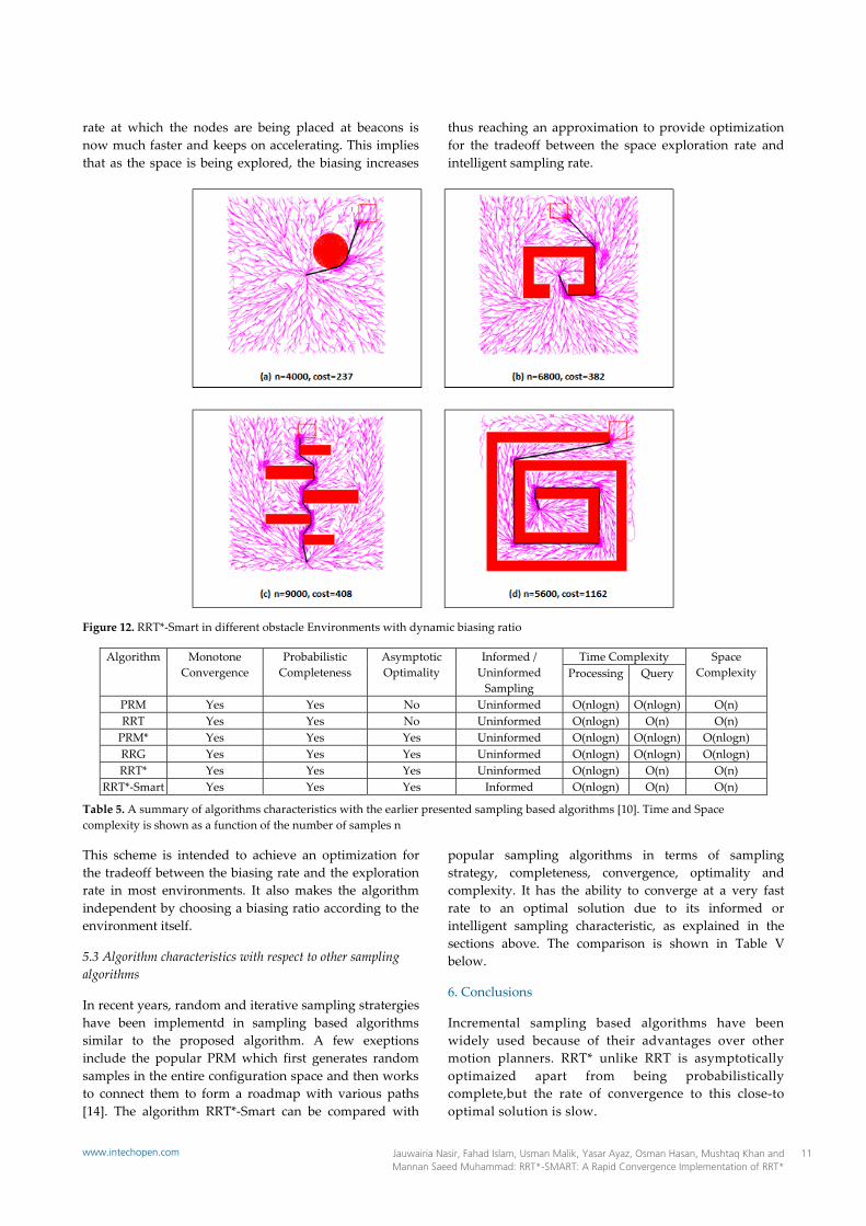
rate at which the nodes are being placed at beacons is now much faster and keeps on accelerating. This implies that as the space is being explored, the biasing increases

thus reaching an approximation to provide optimization for the tradeoff between the space exploration rate and intelligent sampling rate.

Figure 12. RRT*-Smart in different obstacle Environments with dynamic biasing ratio

Algorithm Monotone Convergence

Probabilistic Completeness

Asymptotic Optimality

Informed / Uninformed

Sampling

Time Complexity Space Complexity Processing Query

PRM Yes Yes No Uninformed O(nlogn) O(nlogn) O(n) RRT Yes Yes No Uninformed O(nlogn) O(n) O(n)

PRM* Yes Yes Yes Uninformed O(nlogn) O(nlogn) O(nlogn) RRG Yes Yes Yes Uninformed O(nlogn) O(nlogn) O(nlogn) RRT* Yes Yes Yes Uninformed O(nlogn) O(n) O(n)

RRT*-Smart Yes Yes Yes Informed O(nlogn) O(n) O(n)

Table 5. A summary of algorithms characteristics with the earlier presented sampling based algorithms [10]. Time and Space complexity is shown as a function of the number of samples n

This scheme is intended to achieve an optimization for the tradeoff between the biasing rate and the exploration rate in most environments. It also makes the algorithm independent by choosing a biasing ratio according to the environment itself.

5.3 Algorithm characteristics with respect to other sampling algorithms

In recent years, random and iterative sampling stratergies have been implementd in sampling based algorithms similar to the proposed algorithm. A few exeptions include the popular PRM which first generates random samples in the entire configuration space and then works to connect them to form a roadmap with various paths [14]. The algorithm RRT*-Smart can be compared with

popular sampling algorithms in terms of sampling strategy, completeness, convergence, optimality and complexity. It has the ability to converge at a very fast rate to an optimal solution due to its informed or intelligent sampling characteristic, as explained in the sections above. The comparison is shown in Table V below.

6. Conclusions

Incremental sampling based algorithms have been widely used because of their advantages over other motion planners. RRT* unlike RRT is asymptotically optimaized apart from being probabilistically complete,but the rate of convergence to this close-to optimal solution is slow.


www.intechopen.com

This paper presents a rapid convergence implementation of RRT* known as RRT*-Smart which helps approaching an optimal/near-optimal solution by introducing intelligent sampling and path optimization techniques. Simulation results have demonstrated that RRT*-Smart converges to relatively optimal solutions at very few iterations and at an accelerated rate. Performance comparison proved the efficiency of RRT*-Smart with respect to both time and cost. A natural extention to the proposed work is the generalization to higher dimentional space.

7. Acknowledgements

The authors would like to thank Matthew Walter and Alejandro Perez of CSAIL, Massachusetts Institute of Technology (MIT) for their help and guidance regarding RRT*. The authors are also gratful to National University of Sciences and Technology and Hanyang University Grant (HY-2012-N) for supporting this research.

8. References

[1] M. Kanehara, S. Kagami, J.J. Kuffner, S. Thompson, H. Mizoguhi (2007) "Path shortening and smoothing of grid-based path planning with consideration of obstacles", IEEE International Conference on Systems, Man and Cybernetics, (ISIC) , pp. 991-996.

[2] I. Petrovic and M. Brezak (2011) “A visibility graph based method for path planning in dynamic environments”, in proceedings of 34th International Convention on Information and Commuincation Technology, Electronics and Microelectronics (MIPRO), pp. 711-716.

[3] N.H. Sleumer, N. Tschichold-Grman (1999) “Exact cell decomposition of arrangements used for path planning in robotics”, Technical report. Switzerland: Institute of Theoretical Computer Science Swiss Federal Institute of Technology Zurich.

[4] Y.K.Hwang, N. Ahuja (1992) "A potential field approach to path planning", IEEE Transactions on Robotics and Automation,, vol. 8, no. 1, pp. 23-32.

[5] A. Ghorbani, S, Shiry, and A. Nodehi (2009) ”Using Genetic Algorithm for a Mobile Robot Path Planning”, Proceedings of the 2009 International Conference on Future Computer and Communication (ICFCC) . pp. 164- 166.

[6] S.X. Yang, C. Luo (2004) "A neural network approach to complete coverage path planning", IEEE Transactions on Systems, Man, and Cybernetics, Part B: Cybernetics, vol. 34, no. 1, pp. 718- 724.

[7] Roland Geraerts (2006) “Sampling-based Motion Planning: Analysis and Path Quality”, Ph.D. thesis. Utrecht University.

[8] Roland Geraerts (2006) “On Experimental Research in Sampling-based Motion Planning”, In (IROS) Workshop on Benchmarks in Robotics Research, pp. 31-34.

[9] Lavalle, S.M. (1998). "Rapidly-exploring random trees: A new tool for path planning", Computer Science Dept, Iowa State University, Tech. Rep. TR: 98–11. Retrieved 2008-06-30.S.

[10] S. Karaman and E. Frazzoli (2011) “Sampling-based Algorithms for Optimal Motion Planning”, International Journal of Robotics Research, vol. 30, no. 7, pp. 846-894.

[11] I. Garcia, J. P. How (2005) “Improving the efficiency of Rapidly-exploring Random Trees Using a Potential Function Planner”, in the proceedings of 44th IEEE Conference on Decision and Control, and the European Control Conference, pp. 7965-7970.

[12] Khanmohammadi, S.; Mahdizadeh, A. (2008) "Density Avoided Sampling: An Intelligent Sampling Technique for Rapidly-Exploring Random Trees", Eighth International Conference on Hybrid Intelligent Systems, HIS, pp.672-677.

[13] J. Kuffner and S.M. LaValle (Apr. 2000) RRT-connect: “An efficient approach to single-query path planning”, in Proc. of IEEE Intl. Conf. on Robotics and Automation, pp. 995–1001.

[14] L.E. Kavraki, P.Švestka, J.-C. Latombe, and M.H. Overmars (Aug. 1996) “Probabilistic roadmaps for path planning in high-dimensional configuration spaces”, IEEE Trans. on Robotics and Automation, vol. 12, pp. 566–580.

[15] D. Hsu, J.-C. Latombe, and R. Motwani (1999) “Path planning in expansive configuration spaces”, Intl. J. of Computational Geometry and Applications, vol. 9, no. 4/5, pp. 495–512.

[16] S. M. LaValle and J. J. Kuffner (2001)“Randomized kinodynamic planning,” Intl. J. of Robotics Research, vol. 17, no. 5, pp. 378–400.

[17] I. S¸ucan and L. E. Kavraki (2012) “A sampling-based tree planner for systems with complex dynamics”, IEEE Trans. on Robotics, vol. 28, no. 1, pp.116–131.

[18] S. M. Lavalle and J.J. Kuffner (2000) “Rapidly Exploring Random Trees: Progress and Prospects”, In Proceedings Workshop on the Algorithmic Foundations of Robotics.

[19] S. Karaman, Matthew R. Walter, A. Parez, E. Farazolli and S. Teller (2011) ”Anytime Motion Planning using the RRT”, in proceedings of International Conference on Robotic and Automation, pp. 1478-1483.

[20] M. Zucker, J. Kuffner and M. Branicky (2007) “Multipartite RRTs for Rapid Replanning in Dynamic Environments”, in Proc. Of Internation Conference on Robotics and Automation, pp. 1603-160.

[21] Bialkowski,S. Karaman, and E. Frazzoli (2011) “Massively Parallelizing the RRT and the RRT*,” in Proceedings of the IEEE/RSJ International Conference on Intelligent Robots and Systems (IROS).

[22] Latombe, J.C. (1990) “Robot Motion Planning”, Springer.


rrt*-smart: a rapid convergence implementation of...

Documents