ruggero freddi - uniroma1.it
TRANSCRIPT

Dipartimento di Scienze di Base e Applicate per
l’Ingegneria
PhD thesis in Mathematical Models for
Engineering, Electromagnetism and Nanosciences
Ruggero Freddi
Morse Index of Multiple Blow-UpSolutions to the Two-Dimensional
Sinh-Poisson Equation
Advisors:
Prof. Angela Pistoia
Prof. Massimo Grossi
Academic Years 2016-2019

To my beloved husband Gustavo,
por siempre y para siempre...

Acknowledgements
First, I would like to express my deepest gratitude to my advisors An-
gela Pistoia and Massimo Grossi for the great support, both academic and
human, they gave me over these years as PhD student, for the stimulating
conversations we had, and for the many interesting ideas they shared with
me.
I would also like to thank Federico Amadio Guidi for being a great friend,
as well as for the precious help he gave me, especially in the writing process.
Finally, I would like to thank Alessio Basti and Alice Ramassone for
always being available whenever I needed.
Abstract
In this thesis we consider the Dirichlet problem−∆u = ρ2(eu − e−u) in Ω
u = 0 on ∂Ω,(1)
where ρ is a small parameter and Ω is a C2 bounded domain in R2. For each
ρ sufficiently small, [1] proves the existence of a m-point blow-up solution uρ
jointly with its asymptotic behaviour. We compute the Morse index of uρ in
terms of the Morse index of the associated Hamilton function of this problem.
In addition, we give an asymptotic estimate for the first 4m eigenvalues and
eigenfunctions.
Contents
Introduction and Main Results iii
1 Preliminaries and Notations 1
2 Eigenvalues from 1 to m 8
3 Eigenvalues from m+ 1 to 3m 24
4 Morse Index Computations 62
Bibliography 76
ii
Introduction and Main Results
We are concerned with the study of the Morse index of the Dirichlet
problem −∆u = ρ2(eu − e−u) in Ω
u = 0 on ∂Ω,(2)
where ρ is a small parameter and Ω is a C2 bounded and connected domain in
R2 or a convex polygon with corner points ζ1, . . . , ζn ⊆ ∂Ω. This equation
has been widely studied as it is strictly related to the vortex-type configu-
ration for 2D turbulent Euler flows (see [6], [7], and [24]). Its importance
is due to the fact that, suitably adapted, it describes interesting phenomena
in widely different areas like liquid helium, meteorology and oceanography;
it highlights effects that are important in all those subjects. Moreover, its
dynamics are isomorphic to those of the electrostatic guiding-center plasma,
which have been widely extended to describe strongly magnetized plasmas
(see for instance [34], [29], and [35]).
It has been known since Kirchhoff [21] that, if we let ξi ∈ Ω, i = 1, . . . ,m,
be the centres of the vorticity blobs, then the ξi’s obey an approximate
Hamiltonian dynamic associated to the Hamiltonian function
F(ξ1, . . . , ξm) =1
2
m∑k=1
R(ξk) +1
2
∑16k,j6m
αkαjG(ξk, ξj), (3)
with αk ∈ 1,−1, k = 1, . . . ,m, depending on the sign of the corresponding
vorticity blob. Through two different approaches, Joyce [19] and Montgomery
[28] proved at heuristic level that, if we let ω be the vorticity, ψ the flow’s
iii
iv INTRODUCTION
steam function, β ∈ R the inverse of the temperature, and Z > 0 an appro-
priate normalization constant, then we have ω(ψ) = 2Z
sinh(−ψ) for a flow
with total vorticity equal to zero, i.e.∫
Ωω = 0, and ω(ψ) = 1
Ze−βψ for a flow
with total vorticity equal to one, i.e.∫
Ωω = 1. Setting u = −|β|ψ, the 2D
Euler equation in stationary formw · ∇ω(ψ) = 0 in Ω
−∆ψ = 0 in Ω
w · ν = 0 on ∂Ω \ ζ1, . . . , ζn,
(4)
where w is the velocity field, reduces to the sinh-Poisson equation (2), where
ρ =√|β|Z
. More recently, in [5] and [4] was rigorously proved that for any
β > −9π, ω(ψ) = 1Ze−βψ is the mean field-limit vorticity for both the micro-
canonical and the canonical equilibrium statistic distributions for the Hamil-
tonian point-vortex model. The solutions to (4) with β < 0 of the type of
those suggested in [19] (‘negative temperature’ states) have shown to rapre-
sent very well the numerical experiment on the Navier-Stokes equations with
high Reynolds number ([25], [26], and [30]). For further details and recent
developments in the study of this problem see [4], [22], and [36]. Due to
the just mentioned results much effort has been put into finding out explicit
solutions for the Euler equations with Joy-Montgomery vorticity. Among
the most relevants there are the Mallier-Maslowe [23] counter rotating vor-
tices, and their generalization ([8] and [9]). The Mallier-Maslowe vortices
are sign changing solutions to −∆u = ρ2 sinh(u), with 1-periodic boundary
conditions, one absolute maxima and minima and two nodal domains in each
periodic cell, the resulting Euler flow is composed of symmetric and disjoint
regions where the velocity fields are counter directed. This type of solutions
are a suitable initial data for numerical computations ([36] and [22]). More-
over, their explicit expression led to recent results which gave some insight
of the properties of the non-linear dynamical stabilities of periodic array of
vortices ([20], [18], and [10]).
The Morse index theory is of great importance in many fields, as for

INTRODUCTION v
instance in Physics, where we can look at the Morse index of a solution to an
equation as a measure of the stability of that solution, and in Mathematical
Analysis, as it allows us to determine the number of critical points (see [27],
[31] and [32]).
Different solutions to the equation (2) have been found. In [13] it has been
built a positive solution whose concentration points converges to critical point
of (3), as ρ goes to zero. More recently, in [1] and [3] it has been proved the
existence of a sign changing solution whose velocity field converges to a sum
of Dirac deltas centred at critical points of (3). Furthermore, in [17] it has
been constructed a solution that converges to a sum of k Dirac deltas with
alternate sign all centred at the same critical point of the Robin’s function.
In [1] it is proved that, under some assumptions on the points ξ1, . . . , ξm,
for each ρ sufficiently small there exists a solution uρ to the equation (2),
and its profile is given. Let µρ,j and vρ,j be respectively the j-th eigenvalue
and the j-th eigenfunction of the linearised equation around uρ. Moreover,
let
v(i)ρ,n = χB√8ε
τiρ
(0)(x)vρ,n
(τiρx√
8+ ξρ,i
)be the rescaled function of the n-th eigenfunction around ξρ,i. We begin by
proving some results about the asymptotic behaviour of the eigenvalues µρ,j,
the asymptotic behaviour of the eigenfunctions vρ,j away from the points
ξ1, . . . , ξm, and the asymptotic behaviour of the rescaled eigenfunctions v(i)ρ,j.
We then conclude by giving an expression in term of the Morse index of the
Hamiltonian function for the Morse index of uρ, for ρ suitably small.
Let us now state the main results of this work. We start by the first m
eigenvalues and eigenfunctions
Theorem 0.1. For every j = 1, . . . ,m there exists an k ∈ 1, . . . ,m and
nonzero real constants C(k)j ∈ R such that
1. µρ,j < − 12 log(ρ)
, for ρ small enough;
2. limρ→0 v(k)ρ,j = C
(k)j in C2
loc(R2);

vi INTRODUCTION
3. limρ→0vρ,j(x)
µρ,j= 8π
∑mk=1 C
(k)j G(x, ξk) in C1
loc(Ω \ ξ1, · · · , ξm).
By the previous result we see that the j-th eigenfunction also concentrates
at the points ξk, k = 1, ..,m. If we consider higher eigenvalues, we again
have concentration at k points but a different behaviour occurs. In order
to describe it let us denote by ηj , for j = 1, . . . , 2m, the eigenvalues of the
Hessian matrix of the Hamilton function F at the point (ξ1, . . . , ξm). We will
always work under the assumption that ηj 6= 0, for j = 1, . . . , 2m. Now we
are in position to state the result about the behaviour of µρ,j and vρ,j for
j = m+ 1, .., 3m.
Theorem 0.2. For every j = m + 1, . . . , 3m there exists an k ∈ 1, . . . ,msuch that
1. µρ,j = 1− 3πρ2ηj + o(ρ2), for ρ small enough;
2. limρ→0 v(k)ρ,j =
s(k)1,jx1+s
(k)2,jx2
8+|x|2 in C2loc(R
2) for some s = (s(k)1,j , s
(k)2,j )) 6= (0, 0);
3. limρ→0vρ,jρ
= 2π∑m
k=1τk√
8
(s
(k)1,j
∂G∂x1
(x, ξk) + s(k)2,j
∂G∂x2
(x, ξk))
in C1loc(Ω \
ξ1, . . . , ξm).
Our final results concerns the study of µρ,j and vρ,j for j = 3m, .., 4m.
This result, jointly with the previous theorems, is crucial for the computation
of the Morse index of the solution.
Finally, we have
Theorem 0.3. For every j = 3m+ 1, . . . , 4m there exists an k ∈ 1, . . . ,msuch that
1. µρ,j = 1− 32
1log(ρ)
(1 + o(1)), for ρ small enough;
2. limρ→0 v(k)ρ,j (x) = t
(k)j
8−|x|28+|x|2 in C2
loc(R2) for some t
(k)j 6= 0;
3. log ρ vρ,j(x)→ 2π∑m
k=1 t(k)j G(x, ξk) in C1
loc(Ω \ ξ1, . . . , ξm).
Now let us denote by M(uρ) the Morse index of the solution uρ. We
therefore get our main result.
INTRODUCTION vii
Theorem 0.4. For a sufficiently small ρ we have
M(uρ) = 3m−M(HessF),
where by M(HessF) we denote the number of negative eigenvalues of the
Hessian matrix of F at the point (ξ1, . . . , ξm).
From this, we also deduce that:
Corollary 0.5. For a sufficiently small ρ, we have that
m 6M(uρ) 6 3m.
It’s interesting to notice that the above results are very similar to those
obtained in [15] where the Morse index for the multiple blow-up solutions to
the Gelfand’s problem is calculated and asymptotic estimates for the eigen-
values and eigenfunctions of its associated linearised equation are found.
The biggest difference between this work and [15] is that the solutions to the
Gelfand’s problem can not have sign changing blow-up solutions, while this
type of solutions are possible in our case.
On the other hand, confronting our results with those obtained in [11] we
can see how different they are. In our case, the Morse index of a solution
depends on the Morse index of the Hamiltonian function, while in [11] is
proved that if u is the least energy sign-changing radial solution to−∆u = |u|p−1u in B
u = 0 on ∂B,(5)
where B is the ball of radius one and centred at the origin and p > 1, if p is
large enough, then its Morse index is twelve.
Finally, we want to mention the results obtained in [2] where the equation−∆u = f(u) in Ω
u = 0 on ∂Ω,

viii INTRODUCTION
is studied. In [2] are given proper hypothesis on the regularity and the growth
rate of the non-linear part f for the existence of sign changing solutions with
Morse index at most equal to one and for sign changing solution with Morse
index equal to two.
Before concluding this short introduction the author wants to acknowl-
edge that many of the ideas and the techniques in this thesis have been
inspired by those of [14], where the Morse index is computed for the Gelfand
problem.
Chapter 1
Preliminaries and Notations
In the following work, we will denote by C a constant which may possibly
change from step to step, with o(1) a function of x ∈ R2 and ρ > 0 whose
norm in a suitable function space (which we will specify every time) goes to
zero as ρ goes to zero, and with Ω a C2 bounded and connected domain in
R2 or a convex polygon with corner points ζ1, . . . , ζn ⊆ ∂Ω. Moreover, we
will let ε > 0 be such that B2ε(ξρ,i) ⊆ Ω and B2ε(ξρ,i) ∩B2ε(ξρ,j) = ∅ for any
i, j = 1, . . . ,m and i 6= j, and for ρ > 0 sufficiently small.
We will denote by ψρ,i a function in C∞(R2) such that 0 6 ψρ,i(x) 6 1 and
ψρ,i(x) = 1 for each x in Bε(ξρ,i), and ψρ,i(x) = 0 for each x in R2 \B2ε(ξρ,i).
Furthermore, we will denote by Uτ,ξ the function
Uτ,ξ = log
(8τ 2
(τ 2ρ2 + |x− ξ|2)2
),
solution to −∆U(x) = ρ2eU(x) = 8τ2ρ2
(τ2ρ2+|x−ξ|2)2 x ∈ R2∫R2 eU <∞.
(1.1)
From now on, G(·, ·) and H(·, ·) will denote respectively the Laplacian
Green’s function on Ω and its regular part.
G(x, y) = − 1
2πlog(|x− y|) +H(x, y).
Moreover, we will denote by R the Robin function associated to H, i.e.
R(x) = H(x, x).
1

2 1. Preliminaries and Notations
We will consider the equation−∆u = ρ2(eu − e−u) in Ω
u = 0 on ∂Ω(1.2)
and the Hamilton function
F(x1, . . . , xm) =1
2
m∑k=1
R(xk) +1
2
∑16k,j6m
αkαjG(xk, xj),
with αk ∈ 1,−1.We give the following definition.
Definition 1.1. For any integer k > 1 and any open set U ⊆ Rk, we let
F : U → R be a C1 function, and K ⊆ U be a bounded set of critical points
for F . We will say that K is C1-stable for F if for any Fn → F in C1(U),
there exists at least one critical point yn ∈ U for Fn, and y ∈ K, such that
yn → y as n→∞.
Remark 1. It can be verified that a set K of critical points for F is C1-stable
if either one of the following conditions is satisfied:
(i) K is either a strict local maximum or a strict local minimum set for F ;
(ii) the Brouwer degree deg(∇F,Bε(K), 0) is non-zero, for any ε > 0 small
enough, where Bε(K) = x ∈ U : |x−K| 6 ε.
The following result holds.
Theorem 1.1 ([1, Theorem 1.1]). Let (ξ1, . . . , ξm) be a C1-stable critical
point for the function F . Then, there exist ρ0 > 0 such that for any ρ ∈(0, ρ0), the equation (1.2) has a solution uρ such that
uρ(x)→ 8πm∑k=1
αkG(x, ξk) as ρ→ 0
in C∞loc (Ω \ ξ1, . . . , ξm) ∩ C1,σloc
(Ω \ ξ1, . . . , ξm
), for some σ ∈ (0, 1) and
αk ∈ 1,−1.
3
In [1] it is also proved that the solution of the theorem above has the form
uρ(x) =m∑k=1
αkPUτρ,k,ξρ,k(x) + ϕρ(x), (1.3)
where we denoted by PUτρ,i,ξρ,i the projection of Uτρ,i,ξρ,i onto H10 (Ω). The
parameter point (ξρ,1, . . . , ξρ,m) ∈ Ωm converges to (ξ1, . . . , ξm) ∈ Ωm and
τρ,i =e4π[H(ξρ,i,ξρ,i)+
∑mk=1,k 6=i αiαkG(ξρ,i,ξρ,k)]√
8→ e4π[H(ξi,ξi)+
∑mk=1,k 6=i αiαkG(ξi,ξk)]√
8= τi
(1.4)
as ρ goes to zero. For this reason, τρ,i will be called inappropriately τi. It’s
easy to prove that H(x, ξρ,i) and its derivatives of every order are bounded
in Ω, uniformly in ρ. Let’s set Ui = Uτi,ξi .
We have:
Theorem 1.2 ([1, Theorem 5.2]). Let ϕρ be as in (1.3). Then
limρ→0
ϕρ = 0
in C∞loc(Ω \ ξ1, . . . , ξm) ∩ C1,σ(Ω \ ξ1, . . . , ξm) ∩ C0,α(Ω) ∩W 2,q(Ω), for a
suitable σ ∈ (0, 1), any α ∈ (0, 1), and any q ∈ [1, 2).
and
Theorem 1.3 ([1, Proposition 3.2]). For any p ∈ (1, 43), there exist ρ0 > 0
and R > 0 such that, for any ρ ∈ (0, ρ0), we have ‖ϕρ‖H10 (Ω) 6 Rρ
2−pp | log(ρ)|.
In the following, we will consider β to be a fixed constant in (12, 1). Then,
by the previous theorem, for ρ 1 we have ‖ϕρ‖H10 (Ω) 6 Rρβ| log(ρ)|.
We have:
Theorem 1.4 ([1, Theorem 5.1]). Let PUk be as in (1.3). Then
PUk(x) = Uk(x) + 8πH(x, ξρ,k)− log(8τ 2k ) +O(ρ2)
= log
(1
(τ 2kρ
2 + |x− ξρ,k|2)2
)+ 8πH(x, ξρ,k) +O(ρ2)
in C∞loc(Ω) ∩ C1,σ(Ω).
4 1. Preliminaries and Notations
We will call ξρ,1, . . . , ξρ,m the blow-up points.
We are interested in calculating the Morse index of the solutions to (1.2) of
the form (1.3). The Morse index of a solution u to a differential equation is the
sum of the dimensions of the eigenspaces relative to the negative eigenvalues
of the linearised equation around the solution u.
Let J : H10 (Ω)→ (H1
0 (Ω))∗
be the operator defined as follows
J(u)(v) =
∫Ω
∇u∇v − ρ2
∫Ω
(eu − e−u
)v.
Then uρ, as defined in (1.3), is a weak solution to (1.2) if J(uρ)(v) = 0
for all v ∈ H01 (Ω).
We will denote by L (E,F ) the space of bounded linear operator between
two Banach spaces E and F .
The Frechet derivative J ′uρ ∈ L(H1
0 (Ω), (H10 (Ω))
∗)of J in uρ is defined
as the operator that associates to v ∈ H10 (Ω) the element J ′uρ(v) ∈ (H1
0 (Ω))∗
such that
J ′uρ(v)(w) =
∫Ω
∇v∇w − ρ2
∫Ω
(euρ + e−uρ
)vw, ∀w ∈ H1
0 (Ω). (1.5)
We will denote by (·, ·)H10 (Ω) the standard inner product of H1
0 (Ω).
If the couple (µ, v) is a solution to
J ′uρ(v)(·) = µ(v, ·)H10 (Ω),
that is ∫Ω
∇v∇w − ρ2
∫Ω
(euρ + e−uρ
)vw
= J ′uρ(v)(w)
= µ(v, w)H10 (Ω)
= µ
∫Ω
∇v∇w, ∀w ∈ H10 (Ω),
then µ and v are respectively the eigenvalue and the eigenfunction of the
linearised equation of (1.2) around the solution uρ.
5
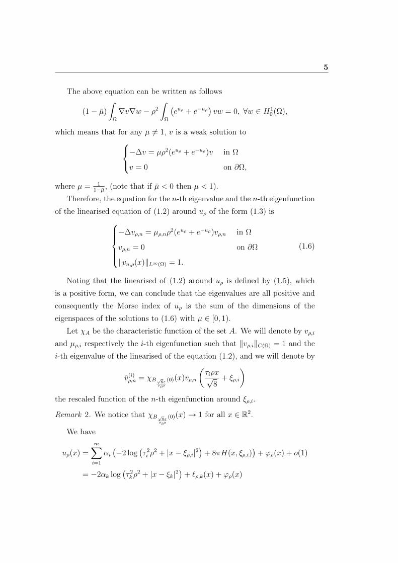
The above equation can be written as follows
(1− µ)
∫Ω
∇v∇w − ρ2
∫Ω
(euρ + e−uρ
)vw = 0, ∀w ∈ H1
0 (Ω),
which means that for any µ 6= 1, v is a weak solution to−∆v = µρ2(euρ + e−uρ)v in Ω
v = 0 on ∂Ω,
where µ = 11−µ , (note that if µ < 0 then µ < 1).
Therefore, the equation for the n-th eigenvalue and the n-th eigenfunction
of the linearised equation of (1.2) around uρ of the form (1.3) is−∆vρ,n = µρ,nρ
2(euρ + e−uρ)vρ,n in Ω
vρ,n = 0 on ∂Ω
‖vn,ρ(x)‖L∞(Ω) = 1.
(1.6)
Noting that the linearised of (1.2) around uρ is defined by (1.5), which
is a positive form, we can conclude that the eigenvalues are all positive and
consequently the Morse index of uρ is the sum of the dimensions of the
eigenspaces of the solutions to (1.6) with µ ∈ [0, 1).
Let χA be the characteristic function of the set A. We will denote by vρ,i
and µρ,i respectively the i-th eigenfunction such that ‖vρ,i‖C(Ω) = 1 and the
i-th eigenvalue of the linearised of the equation (1.2), and we will denote by
v(i)ρ,n = χB√8ε
τiρ
(0)(x)vρ,n
(τiρx√
8+ ξρ,i
)the rescaled function of the n-th eigenfunction around ξρ,i.
Remark 2. We notice that χB√8ετiρ
(0)(x)→ 1 for all x ∈ R2.
We have
uρ(x) =m∑i=1
αi(−2 log
(τ 2i ρ
2 + |x− ξρ,i|2)
+ 8πH(x, ξρ,i))
+ ϕρ(x) + o(1)
= −2αk log(τ 2kρ
2 + |x− ξk|2)
+ `ρ,k(x) + ϕρ(x)

6 1. Preliminaries and Notations
in C∞loc(Ω) ∩ C1,σ(Ω), where
`ρ,k(x) = −2m∑
i=1,i 6=k
αi log(τ 2i ρ
2 + |x− ξρ,i|2)
+ 8πm∑i=1
αiH(x, ξρ,i) + o(1)
in C∞loc(Ω) ∩ C1,σ(Ω). Moreover,
χB 2√
8ετkρ
(0)(x)`ρ,k
(τkρx√
8+ ξρ,k
)= −4
m∑i=1,i 6=k
αi log(|ξk − ξi|) + 8πm∑i=1
αiH(ξk, ξi) + o(1)
= `k + o(1)
in C∞loc(R2) ∩ C1,σ(R2), where
`k = −4m∑
i=1,i 6=k
αi log(|ξk − ξi|) + 8πm∑i=1
αiH(ξi, ξk)
= 8παk
(H(ξk, ξk) + αk
m∑i=1,i 6=k
αi
(− 1
2πlog(|ξk − ξi|) +H(ξi, ξk)
))
= 8παk
(H(ξk, ξk) +
m∑i=1,i 6=k
αkαiG(ξi, ξk)
),
and
χB 2√
8ετkρ
(0)(x)uρ
(τkρx√
8+ ξρ,k
)= χB 2
√8ε
τkρ
(x)
(−4αk log(τkρ)− 2αk log
(1 +|x|2
8
)+
+ `ρ,k
(τkρx√
8+ ξρ,k
)+ ϕρ
(τkρx√
8+ ξρ,k
))
= −4αk log(τkρ)− 2αk log
(1 +|x|2
8
)+ `k(x) + o(1)
in C0,αloc (R2). For the rescaled function of the derivative of uρ we have
χB 2√
8ετkρ
(0)(x)∂uρ∂xi
(τkρx√
8+ ξρ,k
)
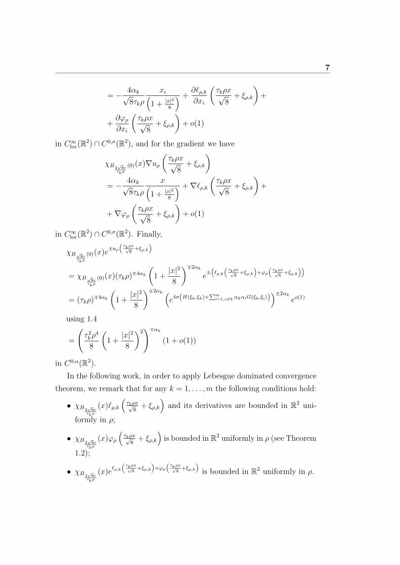
7
= − 4αk√8τkρ
xi(1 + |x|2
8
) +∂`ρ,k∂xi
(τkρx√
8+ ξρ,k
)+
+∂ϕρ∂xi
(τkρx√
8+ ξρ,k
)+ o(1)
in C∞loc(R2) ∩ C0,σ(R2), and for the gradient we have
χB 2√
8ετkρ
(0)(x)∇uρ(τkρx√
8+ ξρ,k
)= − 4αk√
8τkρ
x(1 + |x|2
8
) +∇`ρ,k(τkρx√
8+ ξρ,k
)+
+∇ϕρ(τkρx√
8+ ξρ,k
)+ o(1)
in C∞loc(R2) ∩ C0,σ(R2). Finally,
χB√8ετkρ
(0)(x)e±uρ
(τkρx√
8+ξρ,k
)
= χB√8ετkρ
(0)(x)(τkρ)∓4αk
(1 +|x|2
8
)∓2αk
e±(`ρ,k
(τkρx√
8+ξρ,k
)+ϕρ
(τkρx√
8+ξρ,k
))
= (τkρ)∓4αk
(1 +|x|2
8
)∓2αk (e4π(H(ξk,ξk)+
∑mi=1,i 6=k αkαiG(ξk,ξi))
)±2αkeo(1)
using 1.4
=
(τ 2kρ
4
8
(1 +|x|2
8
)2)∓αk
(1 + o(1))
in C0,α(R2).
In the following work, in order to apply Lebesgue dominated convergence
theorem, we remark that for any k = 1, . . . ,m the following conditions hold:
• χB 2√
8ετkρ
(x)`ρ,k
(τkρx√
8+ ξρ,k
)and its derivatives are bounded in R2 uni-
formly in ρ;
• χB 2√
8ετkρ
(x)ϕρ
(τkρx√
8+ ξρ,k
)is bounded in R2 uniformly in ρ (see Theorem
1.2);
• χB 2√
8ετkρ
(x)e`ρ,k
(τkρx√
8+ξρ,k
)+ϕρ
(τkρx√
8+ξρ,k
)is bounded in R2 uniformly in ρ.

Chapter 2
Eigenvalues from 1 to m
In this chapter, we will study the behaviour of the first m eigenvalues and
eigenfunctions. In particular, we will prove that the first m eigenvalues go
to zero as ρ goes to zero, and hence the Morse index is greater or equal than
m. In addition, we will provide an estimate for the asymptotic behaviour of
the first m eigenfunctions, which will also be of fundamental importance in
the next chapter.
We start by studying the asymptotic behaviour of the eigenfunctions
rescaled around the blow-up points. We prove the following.
Proposition 2.1. The function v(i)ρ,n = χB ε
τiρ(0)(x)v
(τiρx√
8+ ξρ,i
), converges
in C2loc(R
2) to the function v(i)n , solution to the equation
−∆v(i)n (x) = µn
1(1 + |x|2
8
)2 v(i)n (x), x ∈ R2, (2.1)
where µn = limρ→0 µρ,n. Furthermore, there exists at least an i ∈ 1, . . . ,msuch that v
(i)n 6= 0.
8

9
Proof. For any x ∈ B ετiρ
(0) we have
−∆v(i)ρ,n(x)
= −∆
(vn,ρ
(τiρx√
8+ ξρ,i
))=τ 2i ρ
2
8(−∆vρ,n)
(τiρx√
8+ ξρ,i
)= µρ,n
τ 2i ρ
4
8
(euρ(τiρx√
8+ξρ,i
)+ e
−uρ(τiρx√
8+ξρ,i
))vρ,n
(τiρx√
8+ ξρ,i
)
= µρ,neo(1)
1(1 + |x|2
8
)2 +τ 4i ρ
8
64
(1 +|x|2
8
)2
v(i)ρ,n(x).
(2.2)
Note that
τ 4i ρ
8
64
(1 +|x|2
8
)2
6 Cρ8 1
ρ4= o(1), ∀x ∈ B ε
τiρ(0),
and
‖v(i)ρ,n‖2
H10 (R2)
=
∫B ετiρ
(0)
∣∣∇v(i)ρ,n(x)
∣∣2 dx= −
∫B ετiρ
(0)
v(i)ρ,n(x)∆v(i)
ρ,n(x)dx
= µρ,neo(1)
∫B ετiρ
(0)
(v
(i)ρ,n(x)
)2
(1 + |x|2
8
)2dx+
+ µρ,neo(1) τ
4i ρ
8
64
∫B ετiρ
(0)
(1 +|x|2
8
)2 (v(i)ρ,n(x)
)2dx
6 µρ,neo(1)
∫B ετiρ
(0)
1(1 + |x|2
8
)2dx+ µρ,neo(1) τ
4i ρ
8
64
∫B ετiρ
(0)
(1 +|x|2
8
)2
dx
6 8πµρ,n + o(1)
6 C,
(2.3)
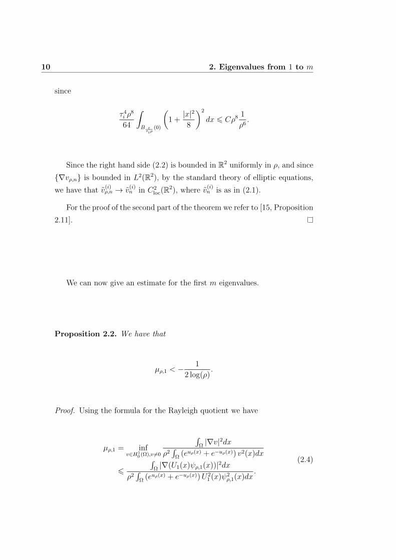
10 2. Eigenvalues from 1 to m
since
τ 4i ρ
8
64
∫B ετiρ
(0)
(1 +|x|2
8
)2
dx 6 Cρ8 1
ρ6.
Since the right hand side (2.2) is bounded in R2 uniformly in ρ, and since
∇vρ,n is bounded in L2(R2), by the standard theory of elliptic equations,
we have that v(i)ρ,n → v
(i)n in C2
loc(R2), where v
(i)n is as in (2.1).
For the proof of the second part of the theorem we refer to [15, Proposition
2.11].
We can now give an estimate for the first m eigenvalues.
Proposition 2.2. We have that
µρ,1 < −1
2 log(ρ).
Proof. Using the formula for the Rayleigh quotient we have
µρ,1 = infv∈H1
0 (Ω),v 6=0
∫Ω|∇v|2dx
ρ2∫
Ω(euρ(x) + e−uρ(x)) v2(x)dx
6
∫Ω|∇(U1(x)ψρ,1(x))|2dx
ρ2∫
Ω(euρ(x) + e−uρ(x))U2
1 (x)ψ2ρ,1(x)dx
.
(2.4)

11
We start by estimating the numerator.
∫Ω
|∇(Ui(x)ψρ,i(x))|2 dx
=
∫Ω
|∇Ui(x)|2 ψ2ρ,i(x)dx+
∫Ω
U2i (x) |∇ψρ,i(x)|2 dx+
+ 2
∫Ω
∇Ui(x)∇ψρ,i(x)Ui(x)ψρ,idx
= −2
∫Ω
∇Ui(x)∇ψρ,i(x)Ui(x)ψρ,i(x)dx−∫
Ω
∆Ui(x)Ui(x)ψ2ρ,i(x)dx+
+
∫Ω
U2i (x)|∇ψρ,i(x)|2dx+ 2
∫Ω
∇Ui(x)∇ψρ,i(x)Ui(x)ψρ,idx
= ρ2
∫Ω
eUi(x)Ui(x)ψ2ρ,i(x)dx+
∫Ω
U2i (x)|∇ψρ,i(x)|2dx
6∫B2ε(ξρ,i)
8τ 2i ρ
2
(τ 2i ρ
2 + |x− ξρ,i|2)2 log
(8τ 2i
(τ 2i ρ
2 + |x− ξρ,i|2)2
)ψ2ρ,i (x) dx+
+ C
∫B2ε(ξρ,i)\Bε(ξρ,i)
U2i (x)dx
=8τ 4i ρ
4
8τ 4i ρ
4∫B 2√
8ετiρ
(0)
(−4 log(ρ)− log
(τ2i
8
)− 2 log
(1 + |x|2
8
))ψ2ρ,i
(τiρx√
8+ ξρ,i
)(
1 + |x|28
)2 dx+ C
using Lebesgue theorem
= 8π
(−4 log(ρ)− log
(τ 2i
8
)− 2
)+ C + o(1)
= −32π log(ρ)(1 + o(1)).
(2.5)

12 2. Eigenvalues from 1 to m
For the denominator we have
ρ2
∫Ω
(euρ(x) + e−uρ(x)
)U2i (x)ψ2
ρ,i(x)dx
> ρ2
∫Bε(ξi,ρ)
(euρ(x) + e−uρ(x)
)U2i (x)dx
= ρ2 τ2i ρ
2
8
∫B√8ετiρ
(0)
(euρ(τiρx√
8+ξρ,i
)+ e
−uρ(τiρx√
8+ξρ,i
))U2i
(τiρx√
8+ ξρ,i
)dx
=τ 2i ρ
4
8
1
τ 4i ρ
4
∫B√8ετiρ
(0)
e`ρ,i
(τiρx√
8+ξρ,i
)+ϕρ
(τiρx√
8+ξρ,i
)(
1 + |x|28
)2
(−4 log(ρ)− log
(τ 2i
8
)− 2 log
(1 +|x|2
8
))2
dx+
+τ 2i ρ
4
8τ 4i ρ
4
∫B√8ετiρ
(0)
e−`ρ,i
(τiρx√
8+ξρ,i
)−ϕρ
(τiρx√
8+ξρ,i
)(1 +|x|2
8
)2
(−4 log(ρ)− log
(τ 2i
8
)− 2 log
(1 +|x|2
8
))2
dx
using Lebesgue theorem
= 16 log2(ρ)
∫R2
dx(1 + |x|2
8
)2 + o(1)
= 128π log2(ρ)(1 + o(1)),
(2.6)
where we used the fact that
τ 6i ρ
8
8
∣∣∣ ∫B√8ετiρ
(0)
e−`ρ,i
(τiρx√
8+ξρ,i
)−ϕρ
(τiρx√
8+ξρ,i
)(1 +|x|2
8
)2
(−4 log(ρ)− log
(τ 2i
8
)− 2 log
(1 +|x|2
8
))2
dx∣∣∣
6 Cρ8 1
ρ6(log(ρ) + 1)2
= o(1).

13
Letting i = 1 in (2.5) and (2.6), and substituting in (2.4), we get
µρ,1 6−32π log(ρ)(1 + o(1))
128π log2(ρ)(1 + o(1))= −1 + o(1)
4 log(ρ)< − 1
2 log(ρ).
Moreover:
Proposition 2.3. We have
1. µρ,j < − 12 log(ρ)
for every j = 1, . . . ,m;
2. v(k)ρ,j → v
(k)j = C
(k)j in C2
loc(R2) for every k, j = 1, . . . ,m;
3. µρ,j 9 0 for every j > m.
Proof. We proceed by induction on m. By Proposition 2.2 we have that
µρ,1 < − 12 log(ρ)
. Let us assume that µρ,j < − 12 log(ρ)
for every j = 1, . . . ,m−1.
By Proposition 2.1 we have that v(k)ρ,j → v
(k)j in C2
loc(R2), and that v
(k)j is a
solution to
−∆v(k)j = 0; x ∈ R2 .
Then v(k)ρ,j → C
(k)j in C2
loc(R2) for every j = 1, . . . ,m − 1 and every k =
1, . . . ,m. Furthermore, we know that there exists k ∈ 1, . . . ,m such that
C(k)j 6= 0. Set
Ψρ(x) =m∑k=1
λkUk(x)ψρ,k(x) +m−1∑k=1
aρ,kvρ,k(x),
where
aρ,j = −(∑m
k=1 λkUkψρ,k, vρ,j)H10 (Ω)
(vρ,j, vρ,j)H10 (Ω)
, (2.7)
for λk ∈ R, and for each j = 1, . . . ,m. It follows immediately that (Ψρ, vρ,j)H10 (Ω) =
0 for every j = 1, . . . ,m− 1.
Let us now show that for a suitable choice of λk, we have aρ,j = o (log(ρ))
for every j = 1, . . . ,m−1. Let us start by estimating the numerator of (2.7).
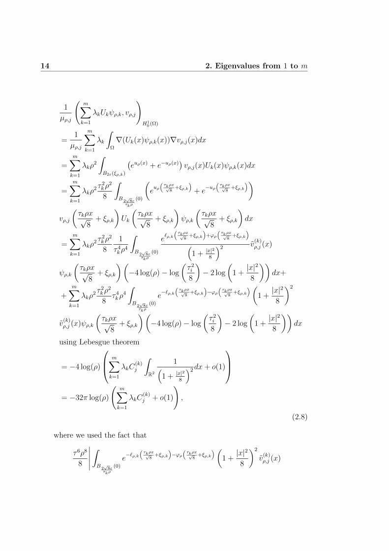
14 2. Eigenvalues from 1 to m
1
µρ,j
(m∑k=1
λkUkψρ,k, vρ,j
)H1
0 (Ω)
=1
µρ,j
m∑k=1
λk
∫Ω
∇(Uk(x)ψρ,k(x))∇vρ,j(x)dx
=m∑k=1
λkρ2
∫B2ε(ξρ,k)
(euρ(x) + e−uρ(x)
)vρ,j(x)Uk(x)ψρ,k(x)dx
=m∑k=1
λkρ2 τ
2kρ
2
8
∫B 2√
8ετkρ
(0)
(euρ(τkρx√
8+ξρ,k
)+ e
−uρ(τkρx√
8+ξρ,k
))
vρ,j
(τkρx√
8+ ξρ,k
)Uk
(τkρx√
8+ ξρ,k
)ψρ,k
(τkρx√
8+ ξρ,k
)dx
=m∑k=1
λkρ2 τ
2kρ
2
8
1
τ 4kρ
4
∫B 2√
8ετkρ
(0)
e`ρ,k
(τkρx√
8+ξρ,k
)+ϕρ
(τkρx√
8+ξρ,k
)(
1 + |x|28
)2 v(k)ρ,j (x)
ψρ,k
(τkρx√
8+ ξρ,k
)(−4 log(ρ)− log
(τ 2i
8
)− 2 log
(1 +|x|2
8
))dx+
+m∑k=1
λkρ2 τ
2kρ
2
8τ 4kρ
4
∫B 2√
8ετkρ
(0)
e−`ρ,k
(τkρx√
8+ξρ,k
)−ϕρ
(τkρx√
8+ξρ,k
)(1 +|x|2
8
)2
v(k)ρ,j (x)ψρ,k
(τkρx√
8+ ξρ,k
)(−4 log(ρ)− log
(τ 2i
8
)− 2 log
(1 +|x|2
8
))dx
using Lebesgue theorem
= −4 log(ρ)
m∑k=1
λkC(k)j
∫R2
1(1 + |x|2
8
)2dx+ o(1)
= −32π log(ρ)
(m∑k=1
λkC(k)j + o(1)
),
(2.8)
where we used the fact that
τ 6ρ8
8
∣∣∣∣∣∫B 2√
8ετkρ
(0)
e−`ρ,k
(τkρx√
8+ξρ,k
)−ϕρ
(τkρx√
8+ξρ,k
)(1 +|x|2
8
)2
v(k)ρ,j (x)

15
ψρ,k
(τkρx√
8+ ξρ,k
)(−4 log(ρ)− log(
τ 2i
8)− 2 log
(1 +|x|2
8
))dx
∣∣∣∣∣6 C
ρ8
ρ6(log(ρ) + 1)
= o(1).
Hence, taking λk such that∑m
k=1 λkC(k)j = 0 for j = 1, . . . ,m− 1, we have
1
µρ,j
(m∑k=1
λkUkψρ,k, vρ,j
)H1
0 (Ω)
= −32π log(ρ)o(1) = o (log(ρ)) . (2.9)
16 2. Eigenvalues from 1 to m
For the denominator we have
‖vρ,j‖2H1
0 (Ω)
= (vρ,j, vρ,j)H10 (Ω)
=
∫Ω
|∇vρ,j(x)|2 dx
= µρ,jρ2
∫Ω
(euρ(x) + e−uρ(x)
)v2ρ,j(x)dx
= µρ,j
(m∑k=1
ρ2
∫Bε(ξρ,k)
(euρ(x) + e−uρ(x)
)v2ρ,j(x)dx+ o(1)
)
= µρ,j
(m∑k=1
ρ2 τ2kρ
2
8
1
τ 4kρ
4∫B√8ετkρ
(0)
e`ρ,k
(τkρx√
8+ξρ,k
)+ϕρ
(τkρx√
8+ξρ,k
)(
1 + |x|28
)2
(v
(k)ρ,j (x)
)2
dx+ o(1)
)+
+ µρ,j
(m∑k=1
ρ2 τ2kρ
2
8τ 4kρ
4
∫B√8ετkρ
(0)
e−`ρ,k
(τkρx√
8+ξρ,k
)−ϕρ
(τkρx√
8+ξρ,k
)(1 +|x|2
8
)2 (v
(k)ρ,j (x)
)2
dx+ o(1)
)
using Lebesgue theorem
= µj
m∑k=1
(C(k)j )2
∫R2
dx(1 + |x|2
8
)2 + o(1)
= 8πµj
(m∑k=1
(C(k)j )2 + o(1)
),
(2.10)
where we used the fact that
τ 6kρ
8
∣∣∣∣∣∣∣∫B√8ετkρ
(0)
e−`ρ,k
(τkρx√
8+ξρ,k
)−ϕρ
(τkρx√
8+ξρ,k
)(1 +|x|2
8
)2 (v
(k)ρ,j (x)
)2
dx
∣∣∣∣∣∣∣6 Cρ8 1
ρ6

17
= o(1).
Using (2.9) and (2.10) in (2.7) we get
aρ,j =o (log(ρ))
8π∑m
i=1
(C
(i)j
)2
+ o(1)= o (log(ρ)) . (2.11)
Using the formula for the Rayleigh quotient, we have
µρ,m = infv∈H1
0 (Ω),v 6=0,v⊥vρ,1,...,v⊥vρ,m−1
∫Ω|∇v|2 dx
ρ2∫
Ω(euρ(x) + e−uρ(x)) v2(x)dx
6
∫Ω|∇Ψρ(x)|2 dx
ρ2∫
Ω(euρ(x) + e−uρ(x)) Ψ2
ρ(x)dx
=
∫Ω
∣∣∇ (∑mk=1 λkUk(x)ψρ,k(x) +
∑m−1k=1 aρ,kvρ,k(x)
)∣∣2 dxρ2∫
Ω(euρ(x) + e−uρ(x))
(∑mk=1 λkUk(x)ψρ,k(x) +
∑m−1k=1 aρ,kvρ,k(x)
)2dx
(2.12)
Let us start by studying the numerator.∫Ω
∣∣∣∣∣∇(
m∑k=1
λkUk(x)ψρ,k(x) +m−1∑k=1
aρ,kvρ,k(x)
)∣∣∣∣∣2
dx
=
∫Ω
∣∣∣∣∣∇(
m∑k=1
λkUk(x)ψρ,k(x)
)∣∣∣∣∣2
dx+
∫Ω
∣∣∣∣∣∇(m−1∑k=1
aρ,kvρ,k(x)
)∣∣∣∣∣2
dx+
+ 2m−1∑j=1
aρ,j
∫Ω
∇
(m∑k=1
λkUk(x)ψρ,k(x)
)∇vρ,j(x)dx
=m∑k=1
λ2k
∫Ω
|∇ (Uk(x)ψρ,k(x))|2 dx+m−1∑k=1
a2ρ,k
∫Ω
|∇vρ,k(x)|2 dx+
+ 2m−1∑j=1
aρ,j
(m∑k=1
λkUkψρ,k, vρ,j
)H1
0 (Ω)
= −32π log(ρ)m∑k=1
λ2k(1 + o(1)).
(2.13)
Since by (2.5) we have∫Ω
|∇ (Uk(x)ψρ,k(x))|2 dx = −32π log(ρ)(1 + o(1)),

18 2. Eigenvalues from 1 to m
by (2.10), (2.11), and since by hypothesis µρ,j < − 12 log(ρ)
, we have
a2ρ,k
∫Ω
|∇vρ,k(x)|2 dx = 8πµja2ρ,k
(m∑k=1
(C
(k)j
)2
+ o(1)
)= o(log(ρ)),
and by (2.9), (2.11), and since by hypothesis µρ,j < − 12 log(ρ)
, we have
aρ,k
(m∑k=1
λkUkψρ,k, vρ,j
)H1
0 (Ω)
= aρ,kµρ,j log(ρ)o(1) = o(log(ρ)).
For the denominator we have
ρ2
∫Ω
(euρ(x) + e−uρ(x)
)( m∑k=1
λkUk(x)ψρ,k(x) +m−1∑k=1
aρ,kvρ,k(x)
)2
dx
= ρ2
∫Ω
(euρ(x) + e−uρ(x)
)( m∑k=1
λkUk(x)ψρ,k(x)
)2
dx+
+ ρ2
∫Ω
(euρ(x) + e−uρ(x)
)(m−1∑k=1
aρ,kvρ,k(x)
)2
dx
+ 2m−1∑j=1
aρ,jρ2
∫Ω
(euρ(x) + e−uρ(x)
)vρ,j(x)
m∑k=1
λkUk(x)ψρ,k(x)dx
=m∑k=1
λ2kρ
2
∫Ω
(euρ(x) + e−uρ(x)
)U2k (x)ψ2
ρ,k(x)dx+
+m∑k=1
a2ρ,kρ
2
∫Ω
(euρ(x) + e−uρ(x)
)v2ρ,k(x)dx
+ 2m−1∑j=1
aρ,j1
µρ,j
(m∑k=1
λkUkψρ,k, vρ,j
)H1
0 (Ω)
= 128 log2(ρ)m∑k=1
λ2k(1 + o(1)),
(2.14)
Since by (2.6) we have
ρ2
∫Ω
(euρ(x) + e−uρ(x)
)Uk(x)2(x)ψ2
ρ,k(x)dx = 128 log2(ρ)(1 + o(1)),
by (2.10), (2.11), and since by hypothesis µρ,j < − 12 log(ρ)
, we have
a2ρ,kρ
2
∫Ω
(euρ(x) + e−uρ(x)
)v2ρ,k(x)dx

19
< −8π1
2 log(ρ)log2(ρ)o(1)
(m∑j=1
(C
(j)k
)2
+ o(1)
)= o(log(ρ)),
and by (2.9) and (2.11), we have
aρ,jµρ,j
(m∑k=1
λkUkψρ,k, vρ,j
)H1
0 (Ω)
= o(log2(ρ)).
Using (2.13) and (2.14) in (2.12) we get
µρ,m 6−32 log(ρ)
∑mk=1 λ
2k(1 + o(1))
128 log2(ρ)∑m
k=1 λ2k(1 + o(1))
< − 1
2 log(ρ).
Since µρ,j → 0 for every j = 1, . . . ,m, proceeding as in the beginning of
this proof we have that v(k)j → C
(k)j in C2
loc(R2) per every k, j = 1, . . . ,m.
Let us finally prove that µρ,i 9 0 for every i > m. Let i and j be such
that µρ,i → 0 and µρ,j → 0, and let Cj = (C(1)j , . . . , C
(n)j ).
By the orthogonality of the eigenfunctions we get
0 = (vρ,i, vρ,j)H10 (Ω) = µρ,iρ
2
∫Ω
(euρ(x) + e−uρ(x)
)vρ,i(x)vρ,j(x)dx,
so that
0 = ρ2
∫Ω
(euρ(x) + e−uρ(x)
)vρ,i(x)vρ,j(x)dx
=m∑k=1
ρ2
∫Bε(ξρ,k)
(euρ(x) + e−uρ(x)
)vρ,i(x)vρ,j(x)dx+ o(1)
=m∑k=1
τ 2kρ
2
8ρ2
∫B√8ετkρ
(0)
(euρ(τkρx√
8+ξρ,k
)+ e
−uρ(τkρx√
8+ξρ,k
))v
(k)ρ,i (x)v
(k)ρ,j (x)dx+ o(1)
=m∑k=1
τ 2kρ
4
8
1
τ 4kρ
4
∫B√8ετkρ
(0)
e`ρ,k
(τkρx√
8+ξρ,k
)+ϕρ
(τkρx√
8+ξρ,k
)(
1 + |x|28
)2 v(k)ρ,i (x)v
(k)ρ,j (x)dx+
+m∑k=1
τ 2kρ
4
8τ 4kρ
4
20 2. Eigenvalues from 1 to m
∫B√8ετkρ
(0)
e−`ρ,k
(τkρx√
8+ξρ,k
)−ϕρ
(τkρx√
8+ξρ,k
)(1 +|x|2
8
)2
v(k)ρ,i (x)v
(k)ρ,j (x)dx+ o(1)
using Lebesgue theorem
= 8πm∑k=1
C(k)i C
(k)j + o(1)
= 8π(Ci, Cj)Rm + o(1),
where we used the fact that∣∣∣∣∣∣∣τ 6kρ
8
8
∫B√8ετkρ
(0)
e−`ρ,k
(τkρx√
8+ξρ,k
)−ϕρ
(τkρx√
8+ξρ,k
)(1 +|x|2
8
)2
v(k)ρ,i (x)v
(k)ρ,j (x)dx
∣∣∣∣∣∣∣6 Cρ8 1
ρ6
= o(1).
Therefore (Ci, Cj)Rm = 0. Since in Rm there are at most m orthogonal
vectors, then there are at most m eigenvalues which go to zero. Since in 1
we proved that the first m eigenvalues go to zero, we get the conclusion.
The next theorem gives an estimate for the asymptotic behaviour of the
first m eigenfunctions away from the blow-up points.
Lemma 2.4. For every 1 6 j 6 m we have
limρ→0
vρ,j(x)
µρ,j= 8π
m∑k=1
C(k)j G(x, ξk)
in C1loc(Ω \ ξ1, . . . , ξm).
Proof. By Proposition 2.3 we know that v(k)ρ,j → C
(k)j in C2
loc(R2) for every
j, k = 1, . . . ,m. For each x ∈ Ω \ ξ1, . . . , ξm, using Green’s representation
21
formula we get
vρ,j(x)
µρ,j= ρ2
∫Ω
(euρ(y) + e−uρ(y)
)vρ,j(y)G(x, y)dy
=m∑k=1
ρ2
∫Bε(ξρ,k)
(euρ(y) + e−uρ(y)
)vρ,j(y)G(x, y)dy + o(1)
=m∑k=1
G(x, ξk)ρ2
∫Bε(ξρ,k)
(euρ(y) + e−uρ(y)
)vρ,j(y)dy+
+m∑k=1
ρ2
∫Bε(ξρ,k)
(euρ(y) + e−uρ(y)
)vρ,j(y)(G(x, y)−G(x, ξk))dy + o(1).
(2.15)
Let us study the integrals in the sums separately. For the first integral we
have
ρ2
∫Bε(ξρ,k)
(euρ(y) + e−uρ(y)
)vρ,j(y)dy
= ρ2 τ2kρ
2
8
1
τ 4kρ
4
∫B√8ετkρ
(0)
e`ρ,k
(τkρx√
8+ξρ,k
)+ϕ(τkρx√
8+ξρ,k
)(
1 + |x|28
)2 v(k)ρ,j (x)dx+
+ ρ2 τ2kρ
2
8τ 4kρ
4
∫B√8ετkρ
(0)
e−`ρ,k
(τkρx√
8+ξρ,k
)−ϕ(τkρx√
8+ξρ,k
)(1 +|x|2
8
)2
v(k)ρ,j (x)dx
using Lebesgue theorem
= C(k)j
∫R2
dx(1 + |x|2
8
)2 + o(1)
= 8πC(k)j + o(1),
(2.16)
where we used the fact that∣∣∣∣∣∣∣τ 6kρ
8
8
∫B√8ετkρ
(0)
e−`ρ,k
(τkρx√
8+ξρ,k
)−ϕ(τkρx√
8+ξρ,k
)(1 +|x|2
8
)2
v(k)ρ,j (x)dx
∣∣∣∣∣∣∣6 Cρ8 1
ρ6
22 2. Eigenvalues from 1 to m
= o(1).
Let us now move to the second integral. For every compact subset K ⊆Ω \ ξρ,1, . . . , ξρ,m and for every k = 1, . . . ,m, there exists ε′k such that, for
ρ small enough, we have
dist(K, ξρ,k) = infx∈K|x− ξρ,k| = ε′ρ,k > ε′k.
Then, for each λ < min(ε, ε′1, . . . , ε′m), if x ∈ K then x /∈ Bλ(ξρ,k). Therefore
ρ2
∫Bε(ξρ,k)
(euρ(y) + e−uρ(y)
)vρ,j(y)(G(x, y)−G(x, ξk))dy
= ρ2
∫Bε(ξρ,k)\Bλ(ξρ,k)
(euρ(y) + e−uρ(y)
)vρ,j(y)(G(x, y)−G(x, ξk))dy+
+ ρ2
∫Bλ(ξρ,k)
(euρ(y) + e−uρ(y)
)vρ,j(y)(G(x, y)−G(x, ξk))dy
= ρ2
∫Bε(ξρ,k)\Bλ(ξρ,k)
(e`ρ,k(y)+ϕρ(y)
(τ 2kρ
2 + |y − ξρ,k|2)2 + e−`ρ,k(y)−ϕρ(y)
(τ 2kρ
2 + |y − ξρ,k|2)2
)vρ,j(y)(G(x, y)−G(x, ξk))dy+
+ ρ2
∫Bλ(ξρ,k)
(euρ(y) + e−uρ(y)
)vρ,j(y)(G(x, y)−G(x, ξk))dy.
For the first of these integrals we have
ρ2
∣∣∣∣∣∫Bε(ξρ,k)\Bλ(ξρ,k)
(e`ρ,k(y)+ϕρ(y)
(τ 2kρ
2 + |y − ξρ,k|2)2 + e−`ρ,k(y)−ϕρ(y)
(τ 2kρ
2 + |y − ξρ,k|2)2
)
vρ,j(y)(G(x, y)−G(x, ξk))dy
∣∣∣∣∣6
(Cρ2
(ρ2 + λ2)2+ Cρ2
)∫Bε(ξρ,k)\Bλ(ξρ,k)
|G(x, y)−G(x, ξk)|dy
since G(x, ·) ∈ L1(Ω)
6 C
(ρ2
(ρ2 + λ2)2+ ρ2
).
Choosing λ = ργ with γ < 12, this integral converges to zero, uniformly in
x ∈ K.

23
Let us now study the second integral.
ρ2
∣∣∣∣∣∫Bλ(ξρ,k)
(euρ(y) + e−uρ(y)
)vρ,j(y)(G(x, y)−G(x, ξk))dy
∣∣∣∣∣6 sup
y∈B(λ)(ξρ,k)
|(G(x, y)−G(x, ξk))|ρ2
∫Bε(ξρ,k)
(euρ(y) + e−uρ(y)
)dy
using the uniform continuity of G in K ×Bε′(ξρ,k) and (2.16)
= o(1).
Therefore
ρ2
∫Bε(ξρ,k)
(euρ(y) + e−uρ(y)
)vρ,j(y)(G(x, y)−G(x, ξk))dy = o(1). (2.17)
Using (2.16) and (2.17) in (2.15) we get
vρ,j(x)
µρ,j= 8π
m∑k=1
C(k)j G(x, ξρ,k) + o(1)
in C0(Ω \ ξ1, . . . , ξm). Using the fact that
∂vρ,j∂xi
= ρ2
∫Ω
(euρ(y) + e−uρ(y)
)vρ,j(y)
∂G
∂xi(x, y)dy,
and proceeding as above, we get the estimate in C1(Ω \ ξ1, . . . , ξm).
Proof of Theorem 0.1. Point 1 of Proposition 2.3 proves 1. Point 2 of Propo-
sition 2.3 proves that
limρ→0
v(k)ρ,j = C
(k)j ,
while Proposition 2.1 proves C(k)j 6= 0 for some k ∈ 1, . . . ,m. Finally,
Lemma 2.4 proves 3.

Chapter 3
Eigenvalues from m + 1 to 3m
In this chapter, we will consider the eigenvalues and the eigenfunctions
from m + 1 to 4m. We will prove that such eigenvalues go to one as ρ
approaches to zero. Being interested in the eigenvalues smaller than one,
we will need to determine if they go to one from below or from above. For
this purpose, we will study the asymptotic behaviour of the eigenfunctions
under different conditions on the behaviour of the eigenfunctions themselves,
rescaled around the blow-up points ξ1, . . . , ξm. Finally, we will prove that
the eigenvalues from 3m+ 1 to 4m go to one from above. This gives that the
Morse Index is smaller or equal than 3m.
We begin by studying the asymptotic behaviour of the eigenfunctions
rescaled around the blow-up points, under the assumption that the relative
eigenvalues are smaller than 1 + o(1). This condition will be proved to hold
for every eigenvalue from m+ 1 to 4m.
We prove the following:
Proposition 3.1. For every j > m, if µρ,j 6 1 + o(1) then µρ,j → 1, and
v(k)ρ,j (x)→ v
(k)j (x) =
s(k)1,jx1 + s
(k)2,jx2
8 + |x|2+ t
(k)j
8− |x|2
8 + |x|2, (3.1)
in C2loc(R
2), and there exists k ∈ 1, . . . ,m such that (s(k)1,j , s
(k)2,j , t
(k)j ) 6=
(0, 0, 0).
24
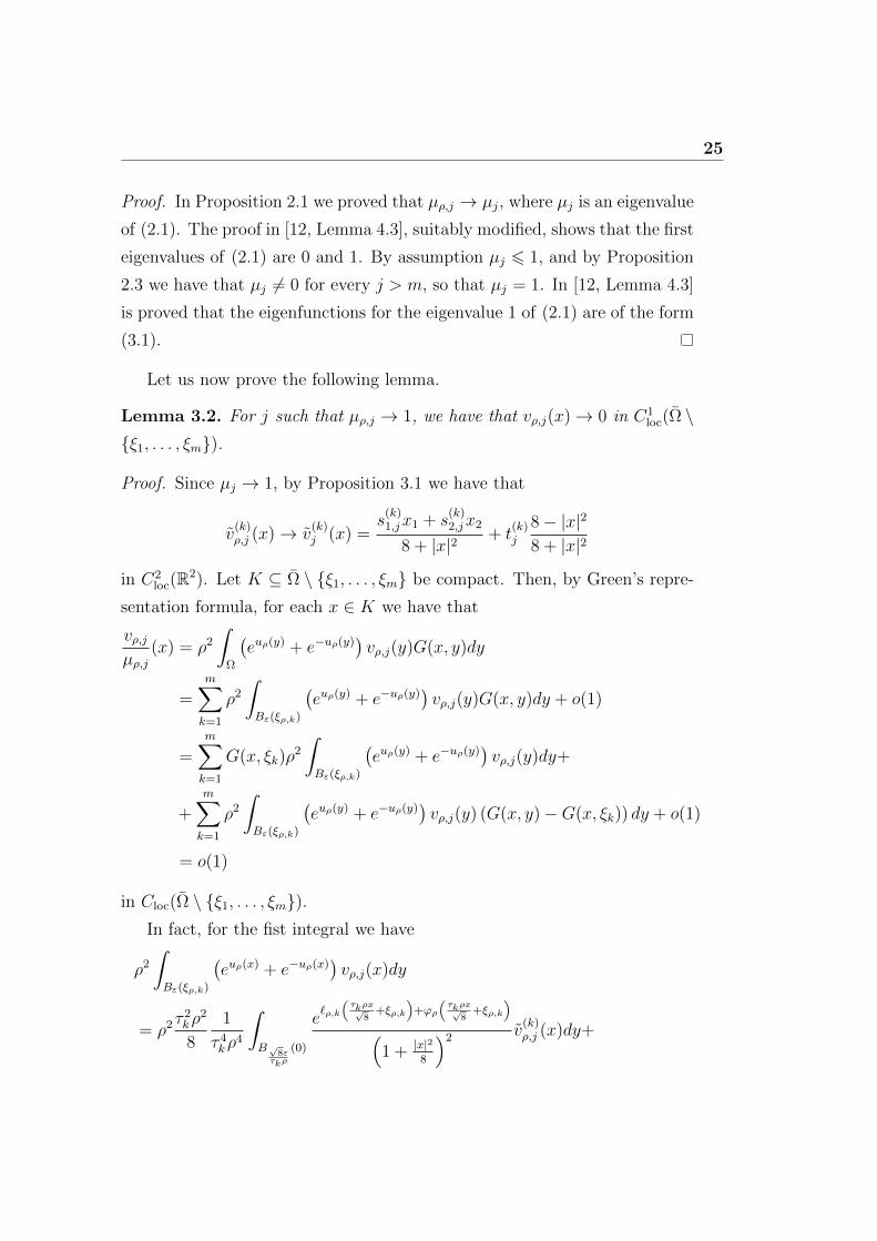
25
Proof. In Proposition 2.1 we proved that µρ,j → µj, where µj is an eigenvalue
of (2.1). The proof in [12, Lemma 4.3], suitably modified, shows that the first
eigenvalues of (2.1) are 0 and 1. By assumption µj 6 1, and by Proposition
2.3 we have that µj 6= 0 for every j > m, so that µj = 1. In [12, Lemma 4.3]
is proved that the eigenfunctions for the eigenvalue 1 of (2.1) are of the form
(3.1).
Let us now prove the following lemma.
Lemma 3.2. For j such that µρ,j → 1, we have that vρ,j(x)→ 0 in C1loc(Ω \
ξ1, . . . , ξm).
Proof. Since µj → 1, by Proposition 3.1 we have that
v(k)ρ,j (x)→ v
(k)j (x) =
s(k)1,jx1 + s
(k)2,jx2
8 + |x|2+ t
(k)j
8− |x|2
8 + |x|2
in C2loc(R
2). Let K ⊆ Ω \ ξ1, . . . , ξm be compact. Then, by Green’s repre-
sentation formula, for each x ∈ K we have that
vρ,jµρ,j
(x) = ρ2
∫Ω
(euρ(y) + e−uρ(y)
)vρ,j(y)G(x, y)dy
=m∑k=1
ρ2
∫Bε(ξρ,k)
(euρ(y) + e−uρ(y)
)vρ,j(y)G(x, y)dy + o(1)
=m∑k=1
G(x, ξk)ρ2
∫Bε(ξρ,k)
(euρ(y) + e−uρ(y)
)vρ,j(y)dy+
+m∑k=1
ρ2
∫Bε(ξρ,k)
(euρ(y) + e−uρ(y)
)vρ,j(y) (G(x, y)−G(x, ξk)) dy + o(1)
= o(1)
in Cloc(Ω \ ξ1, . . . , ξm).In fact, for the fist integral we have
ρ2
∫Bε(ξρ,k)
(euρ(x) + e−uρ(x)
)vρ,j(x)dy
= ρ2 τ2kρ
2
8
1
τ 4kρ
4
∫B√8ετkρ
(0)
e`ρ,k
(τkρx√
8+ξρ,k
)+ϕρ
(τkρx√
8+ξρ,k
)(
1 + |x|28
)2 v(k)ρ,j (x)dy+

26 3. Eigenvalues from m+ 1 to 3m
+ ρ2 τ2kρ
2
8τ 4kρ
4
∫B√8ετkρ
(0)
e−`ρ,k
(τkρx√
8+ξρ,k
)−ϕρ
(τkρx√
8+ξρ,k
)(1 +|x|2
8
)2
v(k)ρ,j (x)dy
using Lebesgue theorem
=
∫R2
1(1 + |x|2
8
)2
(s
(k)1,jx1 + s
(k)2,jx2
8 + |x|2+ t
(k)j
8− |x|2
8 + |x|2
)dx+ o(1)
= o(1),
where we used the fact that
τ 6kρ
8
8
∣∣∣∣∣∣∣∫B√8ετkρ
(0)
e−`ρ,k
(τkρx√
8+ξρ,k
)−ϕρ
(τkρx√
8+ξρ,k
)(1 +|x|2
8
)2
v(k)ρ,j (x)dy
∣∣∣∣∣∣∣6 Cρ8 1
ρ6
= o(1).
For the second integral, proceeding as in the proof of Lemma 2.4, for
every λ < mininfρ,k dist(K, ξρ,k), ε we have
ρ2
∣∣∣∣∣∫Bε(ξρ,k)
(euρ(y) + e−uρ(y)
)vρ,j(y) (G(x, y)−G(x, ξk)) dy
∣∣∣∣∣6 ρ2
∣∣∣∣∣∫Bε(ξρ,k)\Bλ(ξρ,k)
(euρ(y) + e−uρ(y)
)vρ,j(y) (G(x, y)−G(x, ξk)) dy
∣∣∣∣∣++ ρ2
∣∣∣∣∣∫Bλ(ξρ,k)
(euρ(y) + e−uρ(y)
)vρ,j(y) (G(x, y)−G(x, ξk)) dy
∣∣∣∣∣6 C
(ρ2
(ρ2 + λ2)2 + ρ2
)∫Bε(ξρ,k)\Bλ(ξρ,k)
|G(x, y)−G(x, ξk)|dy+
+ supy∈Bλ(ξρ,k)
|G(x, y)−G(x, ξk)|ρ2
∫Bλ(ξρ,k)
(euρ(y) + e−uρ(y)
)dy
using the uniform continuity of G(x, ·) in K, and taking λ = ργ with γ < 12
= o(1)
in Cloc(Ω \ ξ1, . . . , ξm). Using the fact that
∂vρ,j∂xi
(x) = ρ2
∫Ω
(euρ(y) + e−uρ(y)
)vρ,j(y)
∂G
∂xi(x, y)dy,

27
and proceeding as above, we get the estimate in C1loc(Ω \ ξ1, . . . , ξm). We
remark that this also proves that for every j we have
vρ,j(x) = µρ,j
m∑k=1
G(x, ξk)ρ2
∫Bε(ξρ,k)
(euρ(x) + e−uρ(x)
)vρ,j(x)dx+ o(1) (3.2)
in C1loc(Ω \ ξ1, . . . , ξm).
Let us now study the behaviour of the eigenfunctions away from the blow-
up points, under a condition that will be proved to select the eigenfunctions
from 3m+ 1 to 4m.
Lemma 3.3. If µρ,j → 1 and tj = (t(1)j , . . . , t
(m)j ) 6= (0, . . . , 0) then
log(ρ)vρ,j(x)→ 2πm∑k=1
t(k)j G(x, ξk)
in C1loc(Ω \ ξ1, . . . , ξm).
Proof. We have
ρ2
∫Bε(ξρ,k)
(euρ(x) − e−uρ(x)
)vρ,j(x)dx+ o(1)
= ρ2
∫B2ε(ξρ,k)
(euρ(x) − e−uρ(x)
)ψρ,k(x)vρ,j(x)dx+
+
∫B2ε(ξρ,k)\Bε(ξρ,k)
(−∆ψρ,k)(x)uρ(x)vρ,j(x)dx+
+ 2
∫B2ε(ξρ,k)\Bε(ξρ,k)
∇ψρ,k(x)∇uρ(x)vρ,j(x)dx
=
∫Ω
(−∆uρ)(x)ψρ,k(x)vρ,j(x)dx+
∫Ω
(−∆ψρ,k)(x)uρ(x)vρ,j(x)dx+
+ 2
∫Ω
∇ψρ,k(x)∇uρ(x)vρ,j(x)dx
=
∫Ω
−∆(uρ(x)ψρ,k(x))vρ,j(x)dx
=
∫Ω
−∆vρ,j(x)uρ(x)ψρ,k(x)dx
= µρ,jρ2
∫Ω
(euρ(x) + e−uρ(x)
)vρ,j(x)uρ(x)ψρ,k(x)dx
= µρ,jρ2
∫Bε(ξρ,k)
(euρ(x) + e−uρ(x)
)vρ,j(x)uρ(x)dx+ o(1),
(3.3)

28 3. Eigenvalues from m+ 1 to 3m
where we used the fact that ψ and its derivatives are bounded in R2, ‖vρ,j‖C(Ω) 6
1, ‖uρ‖C1(B2ε(ξρ,k)\Bε(ξρ,k)) 6 C, were C doesn’t depend on ρ, and that by
Lemma 3.2 we have vρ,j → 0 in C1loc(Ω \ ξ1, . . . , ξm).
Let us start by studying the first integral. By Proposition 3.1 we know
that
v(k)ρ,j (x)→ v
(k)j (x) =
s(k)1,jx1 + s
(k)2,jx2
8 + |x|2+ t
(k)j
8− |x|2
8 + |x|2
in C2loc(R
2). Hence
ρ2
∫Bε(ξρ,k)
(euρ(x) − e−uρ(x)
)vρ,j(x)dx
= αkρ2 τ
2kρ
2
8
1
τ 4kρ
4
∫B 2√
8ετkρ
(0)
e`ρ,k
(τkρx√
8+ξρ,k
)+ϕρ
(τkρx√
8+ξρ,k
)(
1 + |x|28
)2 v(k)ρ,j (x)dx+
− αkρ2 τ2kρ
2
8τ 4kρ
4
∫B 2√
8ετkρ
(0)
e−`ρ,k
(τkρx√
8+ξρ,k
)−ϕρ
(τkρx√
8+ξρ,k
)(1 +|x|2
8
)2
v(k)ρ,j (x)dx
using Lebesgue theorem
= αk
∫R2
1(1 + |x|2
8
)2
(s
(k)1,jx1 + s
(k)2,jx2
8 + |x|2+ t
(k)j
8− |x|2
8 + |x|2
)dx+ o(1) =
= o(1),
(3.4)
where we used the fact that
τ 6kρ
8
8
∣∣∣∣∣∫B 2√
8ετkρ
(0)
e−`ρ,k
(τkρx√
8+ξρ,k
)−ϕρ
(τkρx√
8+ξρ,k
)(1 +|x|2
8
)2
v(k)ρ,j (x)dx
∣∣∣∣∣6 Cρ8 1
ρ6
= o(1).

29
Let us now study the second integral.
µρ,jρ2
∫Bε(ξρ,k)
(euρ(x) + e−uρ(x)
)vρ,j(x)uρ(x)dx
= µρ,jρ2
∫Bε(ξρ,k)
(euρ(x) + e−uρ(x)
)vρ,j(x)(
−4αk log(τkρ)− 2αk log
(1 +|x− ξρ,k|2
τ 2i ρ
2
)+ `ρ,k(x) + ϕρ(x)
)dx
= −4αk log(τkρ)µρ,jρ2
∫Bε(ξρ,k)
(euρ(x) + e−uρ(x)
)vρ,j(x)dx+
+ µρ,jρ2
∫Bε(ξρ,k)
(euρ(x) + e−uρ(x)
)vρ,j(x)(
−2αk log
(1 +|x− ξρ,k|2
τ 2i ρ
2
)+ `ρ,k(x) + ϕρ(x)
)dx
= −4αk log(τkρ)µρ,jρ2
∫Bε(ξρ,k)
(euρ(x) + e−uρ(x)
)vρ,j(x)dx+
+ µρ,jρ2 τ
2kρ
2
8
1
τ 4kρ
4
∫B√8ετkρ
(0)
e`ρ,k
(τkρx√
8+ξρ,k
)+ϕρ
(τkρx√
8+ξρ,k
)(
1 + |x|28
)2 v(k)ρ,j (x)
(−2αk log
(1 +|x|2
8
)+ `ρ,k
(τkρx√
8+ ξρ,k
)+ ϕρ
(τkρx√
8+ ξρ,k
))dx
+ µρ,jρ2 τ
2kρ
2
8τ 4kρ
4
∫B√8ετkρ
(0)
e−`ρ,k
(τkρx√
8+ξρ,k
)−ϕρ
(τkρx√
8+ξρ,k
)(1 +|x|2
8
)2
v(k)ρ,j (x)
(−2αk log
(1 +|x|2
8
)+ `ρ,k
(τkρx√
8+ ξρ,k
)+ ϕρ
(τkρx√
8+ ξρ,k
))dx
using Lebesgue theorem
= −4αk log(ρ)(1 + o(1))ρ2
∫Bε(ξρ,k)
(euρ(x) + e−uρ(x)
)vρ,j(x)dx+
+
∫R2
1(1 + |x|2
8
)2
(s
(k)1,jx1 + s
(k)2,jx2
8 + |x|2+ t
(k)j
8− |x|2
8 + |x|2
)(−2αk log
(1 +|x|2
8
)+ `k
)dx+ o(1)
= −4αk log(ρ)(1 + o(1))ρ2∫Bε(ξρ,k)
(euρ(x) + e−uρ(x)
)vρ,j(x)dx+ 8παkτ
(k)j + o(1),
(3.5)

30 3. Eigenvalues from m+ 1 to 3m
where we used the fact that
µρ,jτ 6kρ
8
8
∣∣∣∣∣∫B√8ετkρ
(0)
e−`ρ,k
(τkρx√
8+ξρ,k
)−ϕρ
(τkρx√
8+ξρ,k
)(1 +|x|2
8
)2
v(k)ρ,j (x)
(−2αk log
(1 +|x|2
8
)+ `ρ,k
(τkρx√
8+ ξρ,k
)+ ϕρ
(τkρx√
8+ ξρ,k
))dx
∣∣∣∣∣6 Cρ8 1
ρ6(log(ρ) + 1)
= o(1).
Using (3.4) and (3.5) in (3.3) we get
ρ2
∫Bε(ξρ,k)
(euρ(x) + e−uρ(x)
)vρ,j(x)dx =
2πt(k)j + o(1)
log(ρ)(1 + o(1)). (3.6)
Let us now use Green’s representation formula to estimate vρ,j. Let K ⊆Ω \ ξ1, . . . , ξm be compact. Then, for each x ∈ K, we have
log(ρ)vρ,j(x)
= log(ρ)µρ,jρ2
∫Ω
(euρ(y) + e−uρ(y)
)vρ,j(y)G(x, y)dy
= log(ρ)µρ,j
m∑k=1
ρ2
∫Bε(ξρ,k)
(euρ(y) + e−uρ(y)
)vρ,j(y)G(x, y)dy + o(1)
= log(ρ)µρ,j
m∑k=1
G(x, ξk)ρ2
∫Bε(ξρ,k)
(euρ(y) + e−uρ(y)
)vρ,j(y)dy+
+ log(ρ)µρ,j
m∑k=1
ρ2
∫Bε(ξρ,k)
(euρ(y) + e−uρ(y)
)vρ,j(y) (G(x, y)−G(x, ξk)) dy + o(1)
using (3.6)
= 2πm∑k=1
t(k)j G(x, ξk) + o(1),
where we used the fact that, proceeding as in the proof of Lemma 2.4, for
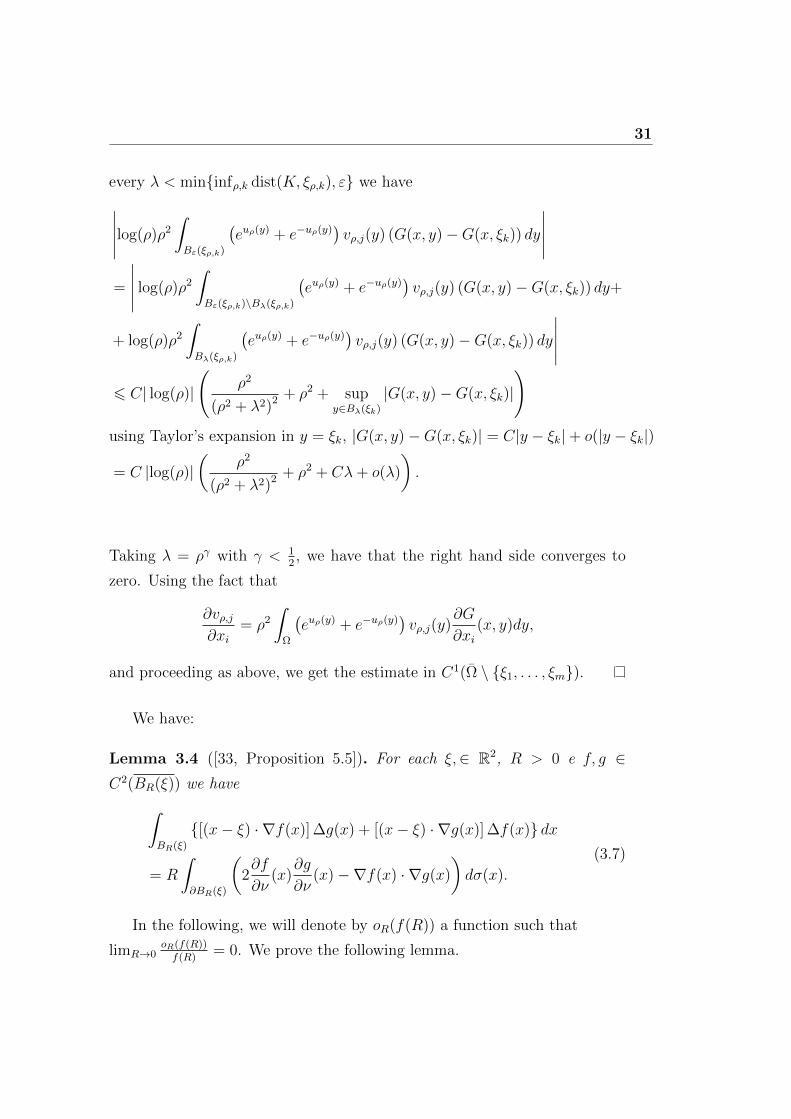
31
every λ < mininfρ,k dist(K, ξρ,k), ε we have∣∣∣∣∣log(ρ)ρ2
∫Bε(ξρ,k)
(euρ(y) + e−uρ(y)
)vρ,j(y) (G(x, y)−G(x, ξk)) dy
∣∣∣∣∣=
∣∣∣∣∣ log(ρ)ρ2
∫Bε(ξρ,k)\Bλ(ξρ,k)
(euρ(y) + e−uρ(y)
)vρ,j(y) (G(x, y)−G(x, ξk)) dy+
+ log(ρ)ρ2
∫Bλ(ξρ,k)
(euρ(y) + e−uρ(y)
)vρ,j(y) (G(x, y)−G(x, ξk)) dy
∣∣∣∣∣6 C| log(ρ)|
(ρ2
(ρ2 + λ2)2 + ρ2 + supy∈Bλ(ξk)
|G(x, y)−G(x, ξk)|
)using Taylor’s expansion in y = ξk, |G(x, y)−G(x, ξk)| = C|y − ξk|+ o(|y − ξk|)
= C |log(ρ)|(
ρ2
(ρ2 + λ2)2 + ρ2 + Cλ+ o(λ)
).
Taking λ = ργ with γ < 12, we have that the right hand side converges to
zero. Using the fact that
∂vρ,j∂xi
= ρ2
∫Ω
(euρ(y) + e−uρ(y)
)vρ,j(y)
∂G
∂xi(x, y)dy,
and proceeding as above, we get the estimate in C1(Ω \ ξ1, . . . , ξm).
We have:
Lemma 3.4 ([33, Proposition 5.5]). For each ξ,∈ R2, R > 0 e f, g ∈C2(BR(ξ)) we have∫
BR(ξ)
[(x− ξ) · ∇f(x)] ∆g(x) + [(x− ξ) · ∇g(x)] ∆f(x) dx
= R
∫∂BR(ξ)
(2∂f
∂ν(x)
∂g
∂ν(x)−∇f(x) · ∇g(x)
)dσ(x).
(3.7)
In the following, we will denote by oR(f(R)) a function such that
limR→0oR(f(R))f(R)
= 0. We prove the following lemma.

32 3. Eigenvalues from m+ 1 to 3m
Lemma 3.5. Let R > 0 be such that BR(ξk)∩BR(ξj) = ∅ e BR(ξk)∩BR(ξi) =
∅. If k 6= j e k 6= i then we have∫∂BR(ξk)
∇G(x, ξi) · ∇G(x, ξj)dσ(x) = oR(1)
and ∫∂BR(ξk)
∂G
∂ν(x, ξi)
∂G
∂ν(x, ξj)dσ(x) = oR(1).
If k = j 6= i or k = i 6= j then we have
R
∫∂BR(ξk)
∇G(x, ξi) · ∇G(x, ξj)dσ(x) = oR(1)
and
R
∫∂BR(ξk)
∂G
∂ν(x, ξi)
∂G
∂ν(x, ξj)dσ(x) = oR(1).
If k = j = i then we have
R
∫∂BR(ξk)
∇G(x, ξi) · ∇G(x, ξj)dσ(x) =1
2π+ oR(1)
and
R
∫∂BR(ξk)
∂G
∂ν(x, ξi)
∂G
∂ν(x, ξj)dσ(x) =
1
2π+ oR(1).
Proof. The case k 6= i and k 6= j is trivial. Let us study the case k = i.
∇G(x, ξk) = − 1
2π
(x− ξk)|x− ξk|2
+∇H(x, ξk),
Then
R
∫∂BR(ξk)
∇G(x, ξk) · ∇G(x, ξj)dσ(x)
= R
∫∂BR(ξk)
(− 1
2π
(x− ξk)|x− ξk|2
+∇H(x, ξk)
)·
·(− 1
2π
(x− ξj)|x− ξj|2
+∇H(x, ξj)
)dσ(x)
= − R2π
∫∂BR(ξk)
(x− ξk)|x− ξk|2
· ∇H(x, ξj)dσ(x)+
+R
4π2
∫∂BR(ξk)
(x− ξk) · (x− ξj)|x− ξk|2|x− ξj|2
dσ(x) + oR(1).

33
Where we used the fact that |∇H(x, ξk)| e∣∣∣ 1
2π
(x−ξj)|x−ξj |2 +∇H(x, ξj)
∣∣∣ are bounded
in BR(ξk) and hence are bounded in ∂BR(ξk), uniformly in R. Let us study
the two integrals separately.
R
2π
∫∂BR(ξk)
(x− ξk)|x− ξk|2
· ∇H(x, ξj)dσ(x)
=R3
2πR2
∫ 2π
0
(cos(θ), sin(θ)) · ∇H(x, ξj)dθ
= oR(1).
Where we used the fact that |∇H(x, ξj)| is bounded in ∂BR(ξk), uniformly
in R. For the second integral we have.
R
4π2
∫∂BR(ξk)
(x− ξk) · (x− ξj)|x− ξk|2|x− ξj|2
dσ(x)
=R3
4π2R2
∫ 2π
0
(cos(θ), sin(θ)) · (R(cos(θ), sin(θ) + (ξk − ξj))|R(cos(θ), sin(θ)) + (ξk − ξj)|2
dθ.
If j 6= k then we have
R3
4π2R2
∫ 2π
0
(cos(θ), sin(θ)) · (R(cos(θ), sin(θ) + (ξk − ξj))|R(cos(θ), sin(θ) + (ξk − ξj)|2
dθ = oR(1),
where we used the fact that the function inside the integral is uniformly
bounded in R. If j = k then we have
R3
4π2R2
∫ 2π
0
(cos(θ), sin(θ)) · (R(cos(θ), sin(θ) + (ξk − ξj))|R(cos(θ), sin(θ) + (ξk − ξj)|2
dθ
=R3
4π2R2
∫ 2π
0
(cos(θ), sin(θ)) · (R(cos(θ), sin(θ))
|R(cos(θ), sin(θ))|2dθ
=R4
4π2R42π
=1
2π.
Analogous computations give the other identities.
The next theorem shows that the hypotheses of Lemma 3.3 do not hold if
the eigenvalues go to one too fast. Thanks to this theorem we will prove that

34 3. Eigenvalues from m+ 1 to 3m
the estimate provided by Lemma 3.3 does not holds for the eigenfunctions
from m+ 1 to 3m, but holds only for the eigenfunctions from 3m+ 1 to 4m .
Theorem 3.6. For every j > m such that µρ,j < 1 + Cρ2, in (3.1) we have
that tj =(t(1)j , . . . , t
(m)j
)= (0, . . . , 0), that is
v(k)ρ,j →
s(k)1,jx1 + s
(k)2,jx2
8 + |x|2
in C2loc(R
2) for some s = (s(k)1,j , s
(k)2,j )) 6= 0. Furthermore, if tj 6= (0, . . . , 0)
then µρ,j > 1.
Proof. By Proposition 3.1 we have that
v(k)ρ,j →
s(k)1,jx1 + s
(k)2,jx2
8 + |x|2+ t
(k)j
8− |x|2
8 + |x|2
in C2loc(R
2). If tj = 0 then s 6= 0, otherwise we would have that v(k)ρ,j → 0. Let
us assume by contradiction that tj 6= 0,that is t(k)j 6= 0 for some k = 1, . . . ,m.
Using (3.7) with f = uρ and g = vρ,j we get
R
∫∂BR(ξk)
(2∂uρ∂ν
(x)∂vρ,j∂ν
(x)−∇uρ(x) · ∇vρ,j(x)
)dσ(x)
=
∫BR(ξk)
[(x− ξk) · ∇uρ(x)] ∆vρ,j(x) + [(x− ξk) · ∇vρ,j(x)] ∆uρ(x) dx.
For the left hand side, by Lemma 3.3 we have
R
∫∂BR(ξk)
(2∂uρ∂ν
(x)∂vρ,j∂ν
(x)−∇uρ(x) · ∇vρ,j(x)
)dσ(x)
= 21
log(ρ)R
∫∂BR(ξk)
∂
∂ν
(8π
m∑i=1
αiG(x, ξi) + o(1)
)∂
∂ν
(2π
m∑n=1
t(n)j G(x, ξn) + o(1)
)dσ(x)+
−R 1
log(ρ)∫∂BR(ξk)
∇
(8π
m∑i=1
αiG(x, ξi) + o(1)
)· ∇
(2π
m∑n=1
t(n)j G(x, ξn) + o(1)
)dσ(x)

35
applying Lemma 3.5
=8π
log(ρ)αkt
(k)j + oR(1).
Let us now study the right hand side.∫BR(ξk)
[(x− ξk) · ∇uρ(x)] ∆vρ,j(x) + [(x− ξk) · ∇vρ,j(x)] ∆uρ(x) dx
= −µρ,jρ2
∫BR(ξk)
[(x− ξk) · ∇uρ(x)](euρ(x) + e−uρ(x)
)vρ,j(x)dx+
− ρ2
∫BR(ξk)
[(x− ξk) · ∇vρ,j(x)](euρ(x) − e−uρ(x)
)dx
= −ρ2
∫BR(ξk)
(x− ξk) · ∇((euρ(x) − e−uρ(x)
)vρ,j(x)
)dx+
− (µρ,j − 1)ρ2
∫BR(ξk)
[(x− ξk) · ∇uρ(x)](euρ(x) + e−uρ(x)
)vρ,j(x)dx
= −ρ2
∫∂BR(ξk)
(x− ξk) · ν(euρ(x) − e−uρ(x)
)vρ,j(x)dσ(x)+
+ 2ρ2
∫BR(ξk)
(euρ(x) − e−uρ(x)
)vρ,j(x)dx+
+ (1− µρ,j)ρ2
∫BR(ξk)
[(x− ξk) · ∇uρ(x)](euρ(x) + e−uρ(x)
)vρ,j(x)dx.
Let us study these three integrals separately. For the first integral we have
− ρ2
∫∂BR(ξk)
(x− ξk) · ν(euρ(x) − e−uρ(x)
)vρ,j(x)dσ(x)
= −Rρ2
∫∂BR(ξk)
(euρ(x) − e−uρ(x)
)vρ,j(x)dσ(x)
= oR(1),
since
ρ2
∣∣∣∣∫∂BR(ξk)
(euρ(x) − e−uρ(x)
)vρ,j(x)dσ(x)
∣∣∣∣6 ρ2
∫BR(ξk)
(euρ(x) + e−uρ(x)
)dx
= ρ2 τ2kρ
2
8
1
τ 4kρ
4
∫√
8Rτkρ
(0)
e`ρ,k
(τkρx√
8+ξρ,k
)+ϕρ
(τkρx√
8+ξρ,k
)(
1 + |x|28
)2 dx+

36 3. Eigenvalues from m+ 1 to 3m
+ ρ2 τ2kρ
2
8τ 4kρ
4
∫√
8Rτkρ
(0)
e−`ρ,k
(τkρx√
8+ξρ,k
)−ϕρ
(τkρx√
8+ξρ,k
)(1 +|x|2
8
)2
dx
using Lebesgue theorem
=
∫R2
dx(1 + |x|2
8
)2 + o(1)
= 8π + o(1),
where we used the fact that
τ 6kρ
8
8
∣∣∣∣∣∫√
8Rτkρ
(0)
e−`ρ,k
(τkρx√
8+ξρ,k
)−ϕρ
(τkρx√
8+ξρ,k
)(1 +|x|2
8
)2
dx
∣∣∣∣∣ 6 Cρ8 1
ρ6= o(1).
For the second integral we have
2ρ2
∫BR(ξk)
(euρ(x) − e−uρ(x)
)vρ,j(x)dx
= αk2ρ2 τ
2kρ
2
8
1
τ 4kρ
4
∫B√8Rτkρ
(0)
e`ρ,k
(τkρx√
8+ξρ,k
)+ϕρ
(τkρx√
8+ξρ,k
)(
1 + |x|28
)2 v(k)ρ,j (x)dx+
+ αk2ρ2 τ
2kρ
2
8τ 4kρ
4
∫B√8Rτkρ
(0)
e−`ρ,k
(τkρx√
8+ξρ,k
)−ϕρ
(τkρx√
8+ξρ,k
)(1 +|x|2
8
)2
v(k)ρ,j (x)dx
using Lebesgue theorem
= 2αk
∫R2
1(1 + |x|2
8
)2
(s
(k)1,jx1 + s
(k)2,jx2
8 + |x|2+ t
(k)j
8− |x|2
8 + |x|2
)dx+ o
(1
log(ρ)
)
= o
(1
log(ρ)
),
where we used the fact that
τ 6kρ
8
8
∣∣∣∣∣∣∣∫B√8Rτkρ
(0)
e−`ρ,k
(τkρx√
8+ξρ,k
)−ϕρ
(τkρx√
8+ξρ,k
)(1 +|x|2
8
)2
v(k)ρ,j (x)dx
∣∣∣∣∣∣∣6 Cρ8 1
ρ6
= o
(1
log(ρ)
).

37
For the third integral we have
ρ2
∫BR(ξk)
[(x− ξk) · ∇uρ(x)](euρ(x) + e−uρ(x)
)vρ,j(x)dx
= ρ2
∫BR(ξk)
(euρ(x) + e−uρ(x)
)vρ,j(x)(x− ξk)·
·(−4αk
(x− ξk)τ 2kρ
2 + |x− ξk|2+∇`ρ,k(x) +∇ϕρ(x)
)dx
= ρ2 τ2kρ
2
8
1
τ 4kρ
4(1 + o(ρ2))
∫B√8Rτkρ
(ξk−ξρ,k)
e`ρ,k
(τkρx√
8+ξρ,k
)+ϕρ
(τkρx√
8+ξρ,k
)(
1 + |x|28
)2 v(k)ρ,j (x)
(−αk
2
|x|2
1 + |x|28
+τkρ√
8x · ∇`ρ,k
(τkρx√
8+ ξρ,k
)+τkρ√
8x · ∇ϕρ
(τkρx√
8+ ξρ,k
))dx+
+ ρ2 τ2kρ
2
8τ 4kρ
4
∫B√8Rτkρ
(ξk−ξρ,k)
e−`ρ,k
(τkρx√
8+ξρ,k
)−ϕρ
(τkρx√
8+ξρ,k
)(1 +|x|2
8
)2
v(k)ρ,j (x)
(−αk
2
|x|2
1 + |x|28
+τkρ√
8x · ∇`ρ,k
(τkρx√
8+ ξρ,k
)+τkρ√
8x · ∇ϕρ
(τkρx√
8+ ξρ,k
))dx
(1 + o (1))
using Lebesgue theorem
= −αk2
∫R2
|x|2(1 + |x|2
8
)3
(s
(k)1,jx1 + s
(k)2,jx2
8 + |x|2+ t
(k)j
8− |x|2
8 + |x|2
)dx+ o (1)
=16
3παkt
(k)j + o (1) ,
where we used the fact that
τ 6kρ
8
8
∣∣∣∣∣∫B√8Rτkρ
(ξk−ξρ,k)
e−`ρ,k
(τkρx√
8+ξρ,k
)−ϕρ
(τkρx√
8+ξρ,k
)(1 +|x|2
8
)2
v(k)ρ,j (x)
(−αk
2
|x|2
1 + |x|28
+τkρ√
8x · ∇`ρ,k
(τkρx√
8+ ξρ,k
))dx
∣∣∣∣∣6 Cρ8 1
ρ6
= o (1) ,
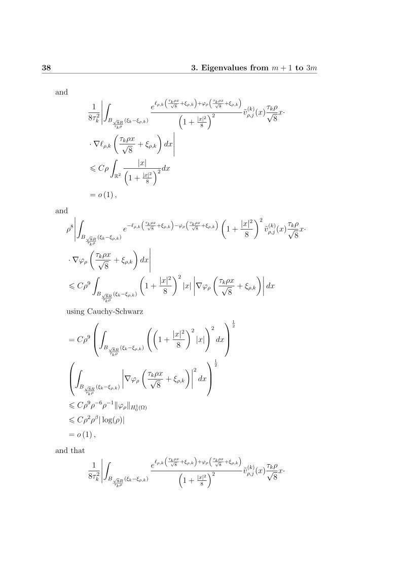
38 3. Eigenvalues from m+ 1 to 3m
and
1
8τ 2k
∣∣∣∣∣∫B√8Rτkρ
(ξk−ξρ,k)
e`ρ,k
(τkρx√
8+ξρ,k
)+ϕρ
(τkρx√
8+ξρ,k
)(
1 + |x|28
)2 v(k)ρ,j (x)
τkρ√8x·
· ∇`ρ,k(τkρx√
8+ ξρ,k
)dx
∣∣∣∣∣6 Cρ
∫R2
|x|(1 + |x|2
8
)2dx
= o (1) ,
and
ρ8
∣∣∣∣∣∫B√8Rτkρ
(ξk−ξρ,k)
e−`ρ,k
(τkρx√
8+ξρ,k
)−ϕρ
(τkρx√
8+ξρ,k
)(1 +|x|2
8
)2
v(k)ρ,j (x)
τkρ√8x·
· ∇ϕρ(τkρx√
8+ ξρ,k
)dx
∣∣∣∣∣6 Cρ9
∫B√8Rτkρ
(ξk−ξρ,k)
(1 +|x|2
8
)2
|x|∣∣∣∣∇ϕρ(τkρx√8
+ ξρ,k
)∣∣∣∣ dxusing Cauchy-Schwarz
= Cρ9
∫B√8Rτkρ
(ξk−ξρ,k)
((1 +|x|2
8
)2
|x|
)2
dx
12
∫B√8Rτkρ
(ξk−ξρ,k)
∣∣∣∣∇ϕρ(τkρx√8+ ξρ,k
)∣∣∣∣2 dx
12
6 Cρ9ρ−6ρ−1‖ϕρ‖H10 (Ω)
6 Cρ2ρβ| log(ρ)|
= o (1) ,
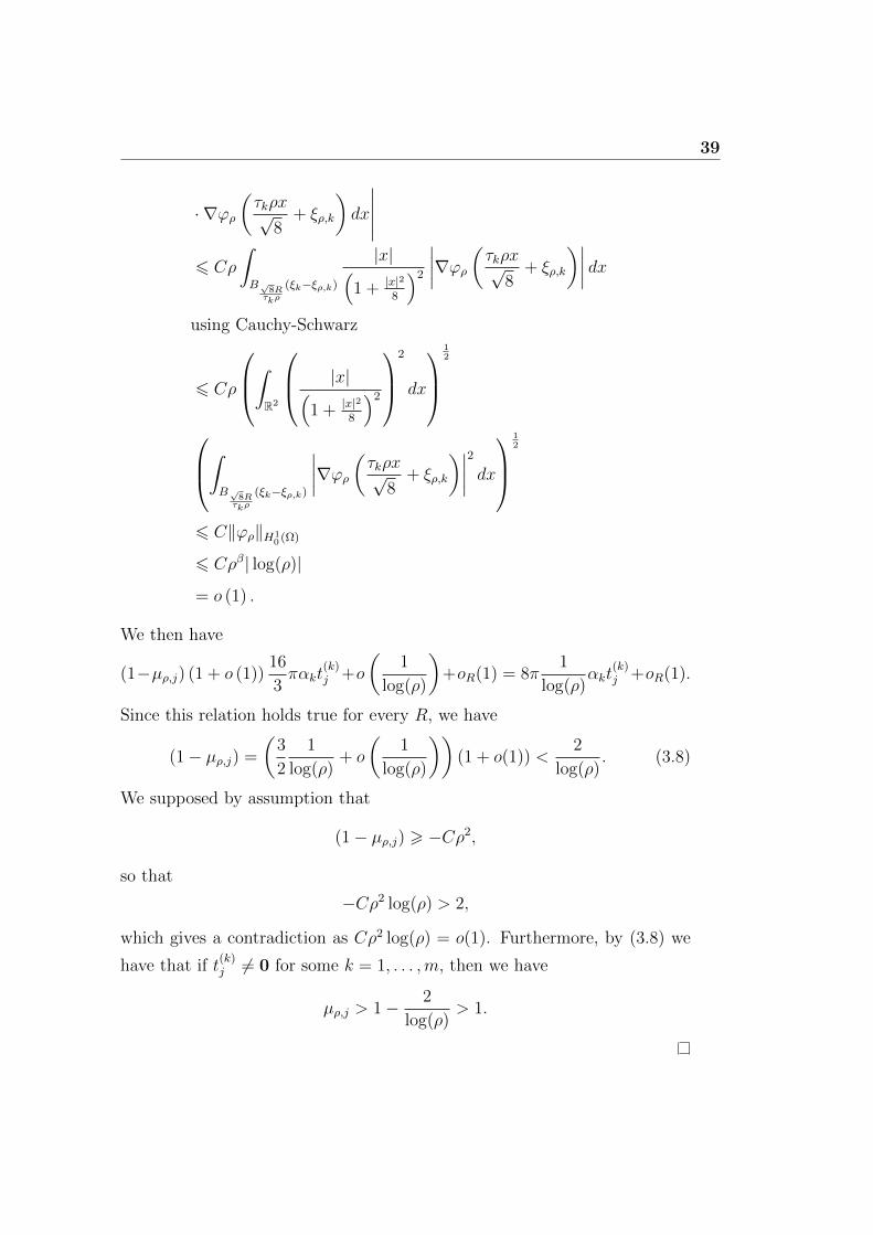
and that
1
8τ 2k
∣∣∣∣∣∫B√8Rτkρ
(ξk−ξρ,k)
e`ρ,k
(τkρx√
8+ξρ,k
)+ϕρ
(τkρx√
8+ξρ,k
)(
1 + |x|28
)2 v(k)ρ,j (x)
τkρ√8x·
39
· ∇ϕρ(τkρx√
8+ ξρ,k
)dx
∣∣∣∣∣6 Cρ
∫B√8Rτkρ
(ξk−ξρ,k)
|x|(1 + |x|2
8
)2
∣∣∣∣∇ϕρ(τkρx√8+ ξρ,k
)∣∣∣∣ dxusing Cauchy-Schwarz
6 Cρ
∫R2
|x|(1 + |x|2
8
)2
2
dx
12
∫B√8Rτkρ
(ξk−ξρ,k)
∣∣∣∣∇ϕρ(τkρx√8+ ξρ,k
)∣∣∣∣2 dx
12
6 C‖ϕρ‖H10 (Ω)
6 Cρβ| log(ρ)|
= o (1) .
We then have
(1−µρ,j) (1 + o (1))16
3παkt
(k)j +o
(1
log(ρ)
)+oR(1) = 8π
1
log(ρ)αkt
(k)j +oR(1).
Since this relation holds true for every R, we have
(1− µρ,j) =
(3
2
1
log(ρ)+ o
(1
log(ρ)
))(1 + o(1)) <
2
log(ρ). (3.8)
We supposed by assumption that
(1− µρ,j) > −Cρ2,
so that
−Cρ2 log(ρ) > 2,
which gives a contradiction as Cρ2 log(ρ) = o(1). Furthermore, by (3.8) we
have that if t(k)j 6= 0 for some k = 1, . . . ,m, then we have
µρ,j > 1− 2
log(ρ)> 1.
40 3. Eigenvalues from m+ 1 to 3m
We prove the following lemma.
Lemma 3.7. For any domain Ω′ ⊆ Ω, and any eigenfunction vρ,n, the fol-
lowing integral identity holds.
(1− µρ,n)ρ2
∫Ω′
(euρ(x) + e−uρ(x)
) ∂uρ∂xj
(x)vρ,n(x)dx
=
∫∂Ω′
∂vρ,n∂ν
(x)∂uρ∂xj
(x)− vρ,n(x)∂2uρ∂ν∂xj
(x)dσx,
(3.9)
where we denoted by ν the extenal normal vector to ∂Ω′.
Proof. Differentiating (1.2) with respect to xj, for j = 1, 2, we get
−∆∂uρ∂xj
(x) = ρ2(euρ(x) + e−uρ(x)
) ∂uρ∂xj
(x), ∀x in Ω.
Multiplying this expression by vρ,n, and integrating both sides of the equation
we get ∫Ω′∇(∂uρ∂xj
)(x)∇vρ,n(x)dx−
∫∂Ω′
vρ,n(x)∂2uρ∂ν∂xj
(x)dσx
= ρ2
∫Ω′
(euρ(x) + e−uρ(x)
) ∂uρ∂xj
(x)vρ,n(x)dx.
On the other hand, multiplying (1.6) by ∂uρ∂xj
we get∫Ω′∇vρ,n∇
(∂uρ∂xj
)(x)dx−
∫∂Ω′
∂vρ,n∂ν
(x)∂uρ∂xj
(x)dσx
= µρ,nρ2
∫Ω′
(euρ(x) + e−uρ(x)
) ∂uρ∂xj
(x)vρ,n(x)dx.
Taking the difference of these two expressions we get the conclusion.
We can now prove that the hypothesis of Theorem 3.6 holds for the eigen-
values from m+ 1 to 3m, and therefore the estimate provided by Lemma 3.3
does not hold for the corresponding eigenfunctions. The next two theorems
show that the eigenvalues from m+ 1 to 3m go to one, give an estimate for
the rate of convergence, and prove that the eigenvalues after 3m are bigger
than one, thus providing an estimate from above for the Morse index.
41
Lemma 3.8. We have that
µρ,m+1 < 1 + Cρ2
and
µρ,m+1 → 1.
Proof. Set
Ψρ(x) =∂uρ∂x1
(x)ψρ,k(x) +m∑j=1
aρ,jvρ,j(x),
where
aρ,j = −
(∂uρ∂x1ψρ,k, vρ,j
)H1
0 (Ω)
(vρ,j, vρ,j)H10 (Ω)
, (3.10)
with k = 1. With this choice for the aρ,j’s we immediately get that Ψρ
is orthogonal to vρ,j for j = 1, . . . ,m. By Proposition 2.3 we have that
µρ,k = o(1) for any k = 1, . . . ,m. Let us prove that aρ,j = o(1). Let us start
by studying the numerator
1
µρ,j
(∂uρ∂x1
ψρ,k, vρ,j
)H1
0 (Ω)
=1
µρ,j
∫Ω
∇(∂uρ∂x1
(x)ψρ,k(x)
)∇vρ,j(x)dx
= ρ2
∫B2ε(ξρ,k)
(euρ(x) + e−uρ(x)
)vρ,j(x)
∂uρ∂x1
(x)ψρ,k(x)dx
= ρ2
∫B2ε(ξρ,k)\Bε(ξρ,k)
(euρ(x) + e−uρ(x)
)vρ,j(x)
∂uρ∂x1
(x)ψρ,k(x)dx+
+ ρ2
∫Bε(ξρ,k)
(euρ(x) + e−uρ(x)
)vρ,j(x)
∂uρ∂x1
(x)dx.
(3.11)
Let us study these integral separately. For the first integral we have
ρ2
∫B2ε(ξρ,k)\Bε(ξρ,k)
(euρ(x) + e−uρ(x)
)vρ,j(x)
∂uρ∂x1
(x)ψρ,k(x)dx = o(1). (3.12)

42 3. Eigenvalues from m+ 1 to 3m
By Lemma 3.7 and Lemma 2.4 we have that
ρ2
∫Bε(ξρ,k)
(euρ(x) + e−uρ(x)
)vρ,j(x)
∂uρ∂x1
(x)dx
=1
1− µρ,j
∫∂Bε(ξρ,k)
(∂vj,ρ∂ν
(x)∂uρ∂x1
(x)− vj,ρ(x)∂2uρ∂ν∂x1
(x)
)dσx
=µρ,j
1− µρ,j(∫∂Bε(ξρ,k))
[∂
∂ν
(8π
m∑k=1
C(k)j G(x, ξk)
)∂
∂x1
(8π
m∑k=1
αkG(x, ξk)
)+
− 8π
(m∑k=1
C(k)j G(x, ξk)
)∂2
∂ν∂x1
(8π
m∑k=1
αkG(x, ξk)
)]dσx + o(1)
)= o(1).
(3.13)
Using (3.12) and (3.13) in (3.11) we get
1
µρ,j
(∂uρ∂x1
ψρ,k, vρ,j
)H1
0 (Ω)
= o(1). (3.14)
By (2.10) we have that
(vρ,j, vρ,j)H10 (Ω) = 8πµρ,j
(m∑k=1
(C
(k)j
)2
+ o(1)
). (3.15)
Using (3.14) and (3.15) in (3.10) we get that aρ,j = o(1). By the formula for
the Rayleigh quotient we have that
µρ,m = infv∈H1
0 (Ω),v 6=0,v⊥vρ,1,...,v⊥vρ,m
∫Ω|∇v|2dx
ρ2∫
Ω(euρ(x) + e−uρ(x)) v2(x)dx
6
∫Ω|∇Ψρ(x)|2dx
ρ2∫
Ω(euρ(x) + e−uρ(x)) Ψ2
ρ(x)dx
=
∫Ω|∇(∂uρ∂x1
(x)ψρ,k(x) +∑m
j=1 aρ,jvρ,j(x))|2dx
ρ2∫
Ω(euρ(x) + e−uρ(x))
(∂uρ∂x1
(x)ψρ,k(x) +∑m
j=1 aρ,jvρ,j(x))2
dx.
(3.16)
Let us start by studying the numerator.∫Ω
∣∣∣∣∣∇(∂uρ∂x1
(x)ψρ,k(x) +m∑j=1
aρ,jvρ,j(x)
)∣∣∣∣∣2
dx

43
=
∫Ω
∣∣∣∣∇(∂uρ∂x1
(x)ψρ,k(x)
)∣∣∣∣2 dx+
∫Ω
∣∣∣∣∣∇(
m∑j=1
aρ,jvρ,j(x)
)∣∣∣∣∣2
dx+
+ 2
∫Ω
∇(∂uρ∂x1
(x)ψρ,k(x)
)∇
(m∑j=1
aρ,jvρ,j(x)
)dx
=
∫Ω
∣∣∣∣∇(∂uρ∂x1
(x)ψρ,k(x)
)∣∣∣∣2 dx+m∑j=1
a2ρ,j
∫Ω
|∇vρ,j(x)|2 dx+
+ 2m∑j=1
aρ,j
(∂uρ∂x1
ψρ,k, vρ,j
)H1
0 (Ω)
=
∫Ω
∣∣∣∣∇(∂uρ∂x1
(x)ψρ,k(x)
)∣∣∣∣2 dx+ o(1)
In fact, by (2.10), and since aρ,k = o(1), we have that
a2ρ,k
∫Ω
|∇vρ,k(x)|2 dx = 8πa2ρ,kµj
(m∑k=1
(C
(k)j
)2
+ o(1)
)= o(1), (3.17)
and by (3.14), and since aρ,k = o(1), we have that
aρ,j
(∂uρ∂x1
ψρ,k, vρ,j
)H1
0 (Ω)
= aρ,jµρ,jo(1) = o(1). (3.18)
We remark that
−∆∂uρ∂x1
(x) = − ∂
∂x1
∆uρ(x)
=∂
∂x1
(ρ2(euρ(x) − e−uρ(x)
))= ρ2
(euρ(x) + e−uρ(x)
) ∂uρ∂x1
(x), ∀x ∈ Ω.
Let us go back to the numerator.∫Ω
∣∣∣∣∇(∂uρ∂x1
(x)ψρ,k(x)
)∣∣∣∣2 dx=
∫Ω
∣∣∣∣∇∂uρ∂x1
(x)
∣∣∣∣2 ψ2ρ,k(x)dx+
∫Ω
∂uρ∂x1
2
(x) |∇ψρ,k(x)|2 dx+
+ 2
∫Ω
∂uρ∂x1
(x)ψρ,k(x)∇∂uρ∂x1
(x)∇ψρ,k(x)dx

44 3. Eigenvalues from m+ 1 to 3m
= −2
∫Ω
∂uρ∂x1
(x)ψρ,k(x)∇∂uρ∂x1
(x)∇ψρ,k(x)dx+
−∫
Ω
∆
(∂uρ∂x1
)(x)
∂uρ∂x1
(x)ψ2ρ,k(x)dx+
+
∫Ω
∂uρ∂x1
2
(x) |∇ψρ,k(x)|2 dx+ 2
∫Ω
∂uρ∂x1
(x)ψρ,k(x)∇∂uρ∂x1
(x)∇ψρ,k(x)dx
= ρ2
∫Ω
(euρ(x) + e−uρ(x)
) ∂uρ∂x1
2
(x)ψ2ρ,k(x)dx+
∫Ω
∂uρ∂x1
2
(x) |∇ψρ,k(x)|2 dx,
hence∫Ω
∣∣∣∣∣∇(∂uρ∂x1
(x)ψρ,k(x) +m∑k=1
aρ,kvρ,k(x)
)∣∣∣∣∣2
dx
= ρ2
∫Ω
(euρ(x) + e−uρ(x)
) ∂uρ∂x1
2
(x)ψ2ρ,k(x)dx+
∫Ω
∂uρ∂x1
2
(x) |∇ψρ,k(x)|2 dx+ o(1).
(3.19)
Let us now study the denominator
ρ2
∫Ω
(euρ(x) + e−uρ(x)
)(∂uρ∂x1
(x)ψρ,k(x) +m∑j=1
aρ,jvρ,j(x)
)2
dx
= ρ2
∫Ω
(euρ(x) + e−uρ(x)
)(∂uρ∂x1
(x)ψρ,k(x)
)2
dx+
+ ρ2
∫Ω
(euρ(x) + e−uρ(x)
)( m∑j=1
aρ,jvρ,j(x)
)2
dx+
+ 2m∑j=1
aρ,jρ2
∫Ω
(euρ(x) + e−uρ(x)
) ∂uρ∂x1
(x)ψρ,k(x)vρ,j(x)dx
= ρ2
∫Ω
(euρ(x) + e−uρ(x)
) ∂uρ∂x1
2
(x)ψ2ρ,k(x)dx+
+m∑j=1
a2ρ,jρ
2
∫Ω
(euρ(x) + e−uρ(x)
)v2ρ,j(x)dx+ 2
m∑j=1
aρ,jµρ,j
(∂uρ∂x1
ψρ,k, vρ,j
)H1
0 (Ω)
= ρ2
∫Ω
(euρ(x) + e−uρ(x)
) ∂uρ∂x1
2
(x)ψ2ρ,k(x)dx+ o(1).
(3.20)
In fact, by (2.10), and since aρ,k = o(1), we have
a2ρ,kρ
2
∫Ω
(euρ(x) + e−uρ(x)
)v2ρ,k(x)dx
45
=a2ρ,k
µρ,j‖vρ,j‖2
H10 (Ω)
= 8πa2ρ,j
(m∑k=1
(C
(k)j
)2
+ o(1)
)= o(1),
and by (3.14), and since aρ,k = o(1), we have
aρ,jµρ,j
(∂uρ∂x1
ψρ,k, vρ,j
)H1
0 (Ω)
= o(1).
Using (3.19) and (3.20) in (3.16), we get
µρ,m 6ρ2∫
Ω
(euρ(x) + e−uρ(x)
) ∂uρ∂x1
2(x)ψ2
ρ,k(x)dx+∫
Ω
∂uρ∂x1
2(x)|∇ψρ,k(x)|2dx+ o(1)
ρ2∫
Ω(euρ(x) + e−uρ(x)) ∂uρ
∂x1
2(x)ψ2
ρ,k(x)dx+ o(1)
= 1 +
∫Ω
∂uρ∂x1
2(x)|∇ψρ,k(x)|2dx+ o(1)
ρ2∫
Ω(euρ(x) + e−uρ(x)) ∂uρ
∂x1
2(x)ψ2
ρ,k(x)dx+ o(1).
It remains to prove that
∫Ω
∂uρ∂x1
2(x)|∇ψρ,k(x)|2dx+ o(1)
ρ2∫
Ω(euρ(x) + e−uρ(x)) ∂uρ
∂x1
2(x)ψ2
ρ,k(x)dx+ o(1)6 Cρ2.
For the numerator we have
∫Ω
∂uρ∂x1
2
(x)|∇ψρ,k(x)|2dx =
∫B2ε(ξρ,k)\Bε(ξρ,k)
∂uρ∂x1
2
(x)|∇ψρ,k(x)|2dx 6 C.

46 3. Eigenvalues from m+ 1 to 3m
For the denominator we have
ρ2
∫Ω
(euρ(x) + e−uρ(x)
) ∂uρ∂x1
2
(x)ψ2ρ,k(x)dx
> ρ2
∫Bε(ξρ,k)
(euρ(x) + e−uρ(x)
) ∂uρ∂x1
2
(x)dx
= ρ2 τ2kρ
2
8
1
τ 4kρ
4
∫B√8ετkρ
(0)
e`ρ,k
(τkρx√
8+ξρ,k
)+ϕρ
(τkρx√
8+ξρ,k
)(
1 + |x|28
)2
(− 4αk√
8τkρ
x1
1 + |x|28
+∂`ρ,k∂x1
(τkρx√
8+ ξρ,k
)+∂ϕρ∂x1
(τkρx√
8+ ξρ,k
))2
dx+
+ ρ2 τ2kρ
2
8τ 4kρ
4
∫B√8ετkρ
(0)
e−`ρ,k
(τkρx√
8+ξρ,k
)−ϕρ
(τkρx√
8+ξρ,k
)(1 +|x|2
8
)2
(− 4αk√
8τkρ
x1
1 + |x|28
+∂`ρ,k∂x1
(τkρx√
8+ ξρ,k
)+∂ϕρ∂x1
(τkρx√
8+ ξρ,k
))2
dx
> ρ2 τ2kρ
2
8
1
τ 4kρ
4
∫B√8ετkρ
(0)
e`ρ,k
(τkρx√
8+ξρ,k
)+ϕρ
(τkρx√
8+ξρ,k
)(
1 + |x|28
)2
(− 4αk√
8τkρ
x1
1 + |x|28
+∂`ρ,k∂x1
(τkρx√
8+ ξρ,k
)+∂ϕρ∂x1
(τkρx√
8+ ξρ,k
))2
dx
>2
τ 2kρ
2
1
8τ 2k
∫B√8ετkρ
(0)
e`ρ,k
(τkρx√
8+ξρ,k
)+ϕρ
(τkρx√
8+ξρ,k
)(
1 + |x|28
)2
x21(
1 + |x|28
)2dx+
−√
8αkτkρ
1
8τ 2k
∫B√8ετkρ
(0)
e`ρ,k
(τkρx√
8+ξρ,k
)+ϕρ
(τkρx√
8+ξρ,k
)(
1 + |x|28
)2
x1
1 + |x|28
∂`ρ,k∂x1
(τkρx√
8+ ξρ,k
)dx+
−√
8αkτkρ
1
8τ 2k
∫B√8ετkρ
(0)
e`ρ,k
(τkρx√
8+ξρ,k
)+ϕρ
(τkρx√
8+ξρ,k
)(
1 + |x|28
)2
x1
1 + |x|28
∂ϕρ∂x1
(τkρx√
8+ ξρ,k
)dx
using Lebesgue theorem
=2
τ 2kρ
2
∫R2
x21(
1 + |x|28
)4dx+ o(1)
=
1
ρ2
(32π
3τ 2k
+ o(1)
),
(3.21)

47
where we used the fact that
1
ρ
∣∣∣∣∣∣∣∫B√8ετkρ
(0)
e`ρ,k
(τkρx√
8+ξρ,k
)+ϕρ
(τkρx√
8+ξρ,k
)(
1 + |x|28
)2
x1
1 + |x|28
∂`ρ,k∂x1
(τkρx√
8+ ξρ,k
)dx
∣∣∣∣∣∣∣6C
ρ
∫R2
|x|(1 + |x|2
8
)3dx
<C
ρ,
and that
1
ρ
∣∣∣∣∣∣∣∫B√8ετkρ
(0)
e`ρ,k
(τkρx√
8+ξρ,k
)+ϕρ
(τkρx√
8+ξρ,k
)(
1 + |x|28
)2
x1
1 + |x|28
∂ϕρ∂x1
(τkρx√
8+ ξρ,k
)dx
∣∣∣∣∣∣∣6C
ρ
∫B√8ετkρ
(0)
|x1|(1 + |x|2
8
)3
∣∣∣∣∂ϕρ∂x1
(τkρx√
8+ ξρ,k
)∣∣∣∣ dxusing Cauchy-Schwarz
6C
ρ
∫B√8ετkρ
(0)
|x1|(1 + |x|2
8
)3
2
dx
12∫
B√8ετkρ
(0)
∣∣∣∣∂ϕρ∂x1
(τkρx√
8+ ξρ,k
)∣∣∣∣2 dx
12
6C
ρ2‖ϕρ‖H1
0 (Ω)
6C
ρ2ρβ log(ρ)
=1
ρ2o(1).
Therefore∫Ω
∂uρ∂x1
2(x)|∇ψρ,k(x)|2dx+ o(1)
ρ2∫
Ω(euρ(x) + e−uρ(x)) ∂uρ
∂x1
2(x)ψ2
ρ,k(x)dx+ o(1)6
C
1ρ2
∑mk=1
(32π3τ2k
+ o(1)) 6 Cρ2.
Proposition 3.9. We have
(i) µρ,j 6 1 + Cρ2 for every m+ 1 6 j 6 3m;

48 3. Eigenvalues from m+ 1 to 3m
(ii) µρ,j → 1 for every m+ 1 6 j 6 3m ;
(iii) µρ,j > 1 for every j > 3m.
Proof. Let us start by proving (i). Let us proceed by induction on m. We
know that (i) holds true for j = m+ 1. Let us assume that it holds true for
m+ 1 6 j 6 3m− 1. We show now that it holds true for j = 3m.
Set
Ψρ(x) =m∑k=1
(λ
(k)1
∂uρ∂x1
(x) + λ(k)2
∂uρ∂x2
(x)
)ψρ,k(x) +
3m−1∑j=1
aρ,jvρ,j(x),
where
aρ,j = −
(∑mk=1
(λ
(k)1
∂uρ∂x1
+ λ(k)2
∂uρ∂x2
)ψρ,k, vρ,j
)H1
0 (Ω)
(vρ,j, vρ,j)H10 (Ω)
= −
∑mk=1 λ
(k)1
(∂uρ∂x1ψρ,k, vρ,j
)H1
0 (Ω)
(vρ,j, vρ,j)H10 (Ω)
−
∑mk=1 λ
(k)2
(∂uρ∂x2ψρ,k, vρ,j
)H1
0 (Ω)
(vρ,j, vρ,j)H10 (Ω)
,
(3.22)
for m+ 1 6 j 6 3m− 1. With this choice for the aρ,j’s it is immediate to see
that Ψρ is orthogonal to vρ,j for 1 6 j 6 3m−1. We have seen in Lemma 3.8
that aρ,j = o(1) for every j 6 m. Let us now prove that, for a suitable choice
of the λk1’s and λ(k)2 ’s we have ρaρ,j = o(1) for every m+ 1 6 j 6 3m− 1. By
inductive hypothesis and by Theorem 3.6, for every m+ 1 6 j 6 3m− 1 and
every k = 1, . . . ,m we have that
v(k)ρ,j →
s(k)1,jx1 + s
(k)2,jx2
8 + |x|2

49
in C2loc(R
2). Let us start by studying the numerator of (3.22).(m∑k=1
(λ
(k)1
∂uρ∂x1
+ λ(k)2
∂uρ∂x2
)ψρ,k, vρ,j
)H1
0 (Ω)
=m∑k=1
∫Ω
∇((
λ(k)1
∂uρ∂x1
(x) + λ(k)2
∂uρ∂x2
(x)
)ψρ,k(x)
)∇vρ,j(x)dx
=m∑k=1
µρ,jρ2
∫B2ε(ξρ,k)
(euρ(x) + e−uρ(x)
)vρ,j(x)
(λ
(k)1
∂uρ∂x1
(x) + λ(k)2
∂uρ∂x2
(x)
)ψρ,k(x)dx
=m∑k=1
µρ,jρ2 τ
2kρ
2
8
1
τ 4kρ
4∫B 2√
8ετkρ
(0)
e`ρ,k
(τkρx√
8+ξρ,k
)+ϕρ
(τkρx√
8+ξρ,k
)(
1 + |x|28
)2 v(k)ρ,j (x)ψρ,k
(τkρx√
8+ ξρ,k
)(− 4αk√
8τkρ
λ(k)1 x1 + λ
(k)2 x2
8 + |x|2+
(λ
(k)1
∂`ρ,k∂x1
+ λ(k)2
∂`ρ,k∂x2
)(τkρx√
8+ ξρ,k
)+
+
(λ
(k)1
∂ϕρ∂x1
+ λ(k)2
∂ϕρ∂x2
)(τkρx√
8+ ξρ,k
))dx+
+m∑k=1
µρ,jρ2 τ
2kρ
2
8τ 4kρ
4
∫B 2√
8ετkρ
(0)
e−`ρ,k
(τkρx√
8+ξρ,k
)−ϕρ
(τkρx√
8+ξρ,k
)(1 +|x|2
8
)2
v(k)ρ,j (x)
ψρ,k
(τkρx√
8+ ξρ,k
)(− 4αk√
8τkρ
λ(k)1 x1 + λ
(k)2 x2
8 + |x|2+(
λ(k)1
∂`ρ,k∂x1
+ λ(k)2
∂`ρ,k∂x2
)(τkρx√
8+ ξρ,k
)+(
λ(k)1
∂ϕρ∂x1
+ λ(k)2
∂ϕρ∂x2
)(τkρx√
8+ ξρ,k
))dx
=m∑k=1
µρ,jρ2 τ
2kρ
2
8
1
τ 4kρ
4∫B 2√
8ετkρ
(0)
e`ρ,k
(τkρx√
8+ξρ,k
)+ϕρ
(τkρx√
8+ξρ,k
)(
1 + |x|28
)2 v(k)ρ,j (x)ψρ,k
(τkρx√
8+ ξρ,k
)(− 4αk√
8τkρ
λ(k)1 x1 + λ
(k)2 x2
8 + |x|2+
(λ
(k)1
∂`ρ,k∂x1
+ λ(k)2
∂`ρ,k∂x2
)(τkρx√
8+ ξρ,k
))dx+
+ µρ,jo(1)
ρ,
(3.23)
50 3. Eigenvalues from m+ 1 to 3m
where we used the fact that
τ 6kρ
8
8
∣∣∣∣∣∫B 2√
8ετkρ
(0)
e−`ρ,k
(τkρx√
8+ξρ,k
)−ϕρ
(τkρx√
8+ξρ,k
)(1 +|x|2
8
)2
v(k)ρ,j (x)ψρ,k
(τkρx√
8+ ξρ,k
)(− 4αk√
8τkρ
λ(k)1 x1 + λ
(k)2 x2
8 + |x|2+
(λ
(k)1
∂`ρ,k∂x1
+ λ(k)2
∂`ρ,k∂x2
)(τkρx√
8+ ξρ,k
))dx
∣∣∣∣∣6 Cρ8 1
ρ6
= o(1),
and∣∣∣∣∣∫B 2√
8ετkρ
(0)
e`ρ,k
(τkρx√
8+ξρ,k
)+ϕρ
(τkρx√
8+ξρ,k
)(
1 + |x|28
)2 v(k)ρ,j (x)
ψρ,k
(τkρx√
8+ ξρ,k
)∂ϕρ∂xi
(τkρx√
8+ ξρ,k
)dx
∣∣∣∣∣6 C
∫B 2√
8ετkρ
(0)
1(1 + |x|2
8
)2
∣∣∣∣∂ϕρ∂xi
(τkρx√
8+ ξρ,k
)∣∣∣∣ dxusing Cauchy-Schwarz
6 C
∫B 2√
8ετkρ
(0)
1(1 + |x|2
8
)2
2
dx
12∫
B 2√
8ετkρ
(0)
∣∣∣∣∂ϕρ∂xi
(τkρx√
8+ ξρ,k
)∣∣∣∣2 dx
12
6C
ρ‖ϕρ‖H1
0 (Ω)
6C
ρρβ| log(ρ)|
=o(1)
ρ,
and that
ρ8
∣∣∣∣∣∫B 2√
8ετkρ
(0)
e−`ρ,k
(τkρx√
8+ξρ,k
)−ϕρ
(τkρx√
8+ξρ,k
)(1 +|x|2
8
)2
v(k)ρ,j (x)ψρ,k
(τkρx√
8+ ξρ,k
)∂ϕρ∂xi
(τkρx√
8+ ξρ,k
)dx
∣∣∣∣∣

51
6 Cρ8
∫B 2√
8ετkρ
(0)
(1 +|x|2
8
)2 ∣∣∣∣∂ϕρ∂xi
(τkρx√
8+ ξρ,k
)∣∣∣∣ dxusing Cauchy-Schwarz
6 Cρ8
∫B 2√
8ετkρ
(0)
(1 +|x|2
8
)4
dx
12∫
B 2√
8ετkρ
(0)
∣∣∣∣∂ϕρ∂xi
(τkρx√
8+ ξρ,k
)∣∣∣∣2 dx
12
6 Cρ2‖ϕρ‖H10 (Ω)
6 Cρ2ρβ| log(ρ)|
= o(1).
Moreover,
m∑k=1
µρ,jρ2 τ
2kρ
2
8
1
τ 4kρ
4∫B 2√
8ετkρ
(0)
e`ρ,k
(τkρx√
8+ξρ,k
)+ϕρ
(τkρx√
8+ξρ,k
)(
1 + |x|28
)2 v(k)ρ,j (x)ψρ,k
(τkρx√
8+ ξρ,k
)(− 4αk√
8τkρ
λ(k)1 x1 + λ
(k)2 x2
8 + |x|2+
(λ
(k)1
∂`ρ,k∂x1
+ λ(k)2
∂`ρ,k∂x2
)(τkρx√
8+ ξρ,k
))dx+
+ µρ,jo(1)
ρ
using Lebesgue theorem
=m∑k=1
− 4αk√8τkρ
µρ,j
∫R2
1(1 + |x|2
8
)2
s(k)1,jx1 + s
(k)2,jx2
8 + |x|2λ
(k)1 x1 + λ
(k)2 x2
8 + |x|2dx(1 + o(1))+
+m∑k=1
µρ,j
(λ
(k)1
∂`ρ,k∂x1
(ξk) + λ(k)2
∂`ρ,k∂x2
(ξk)
)∫R2
1(1 + |x|2
8
)2
s(k)1,jx1 + s
(k)2,jx2
8 + |x|2dx+ µρ,j
o(1)
ρ
= − π
3√
8µρ,j
1
ρ
m∑k=1
αkτk
(s
(k)1,jλ
(k)1 + s
(k)2,jλ
(k)2
)(1 + o(1)) + µρ,j
o(1)
ρ
taking λ(k)1 and λ
(k)2 such that
∑mk=1
αkτk
(s
(k)1,jλ
(k)1 + s
(k)2,jλ
(k)2
)= 0

52 3. Eigenvalues from m+ 1 to 3m
= µρ,jo(1)
ρ.
Then, if m+ 1 6 j 6 3m− 1 we have(m∑k=1
(λ
(k)1
∂uρ∂x1
+ λ(k)2
∂uρ∂x2
)ψρ,k, vρ,j
)H1
0 (Ω)
= µρ,jo(1)
ρ. (3.24)
For the denominator of (3.22), for m+ 1 6 j 6 3m− 1 we have
(vρ,j, vρ,j)H10 (Ω)
=
∫Ω
|∇vρ,j(x)|2dx
= µρ,jρ2
∫Ω
(euρ(x) + e−uρ(x)
)v2ρ,j(x)dx
= µρ,j
m∑k=1
ρ2 τ2kρ
2
8
1
τ 4kρ
4
∫B√8ετkρ
(0)
e`ρ,k
(τkρx√
8+ξρ,k
)+ϕρ
(τkρx√
8+ξρ,k
)(
1 + |x|28
)2
(v
(k)ρ,j (x)
)2
dx+
+ µρ,j
m∑k=1
ρ2 τ2kρ
2
8τ 4kρ
4
∫B√8ετkρ
(0)
e−`ρ,k
(τkρx√
8+ξρ,k
)−ϕρ
(τkρx√
8+ξρ,k
)(1 +|x|2
8
)2 (v
(k)ρ,j (x)
)2
dx+ o(1)
using Lebesgue theorem
= µρ,j
m∑k=1
∫R2
1(1 + |x|2
8
)2
(s
(k)1,jx1 + s
(k)2,jx2
8 + |x|2
)2
dx+ o(1)
=π
12µρ,j
m∑k=1
((s
(k)1,j
)2
+(s
(k)2,j
)2)
+ o(1),
(3.25)
where we used the fact that
τ 6kρ
8
8
∣∣∣∣∣∣∣∫B√8ετkρ
(0)
e−`ρ,k
(τkρx√
8+ξρ,k
)−ϕρ
(τkρx√
8+ξρ,k
)(1 +|x|2
8
)2 (v
(k)ρ,j (x)
)2
dx
∣∣∣∣∣∣∣6 Cρ8 1
ρ6

53
Using (3.24) and (3.25) in (3.22) we get that for m + 1 6 j 6 3m − 1, we
have ρaρ,j = o(1). By the formula for the Rayleigh quotient we get that
µρ,3m = infv∈H1
0 (Ω),v 6=0,v⊥vρ,1,...,v⊥vρ,3m−1
∫Ω|∇v|2dx
ρ2∫
Ω(euρ(x) + e−uρ(x)) v2(x)dx
6
∫Ω|∇Ψρ(x)|2dx
ρ2∫
Ω(euρ(x) + e−uρ(x)) Ψ2
ρ(x)dx
=N
D.
(3.26)
Where
N =
∫Ω
∣∣∣∣∣∇(
m∑k
(λ
(k)1
∂uρ∂x1
(x) + λ(k)2
∂uρ∂x2
(x)
)ψρ,k(x) +
3m−1∑j=1
aρ,jvρ,j(x)
)∣∣∣∣∣2
dx
and
D = ρ2
∫Ω
(euρ(x) + e−uρ(x)
)(
m∑k
(λ
(k)1
∂uρ∂x1
(x) + λ(k)2
∂uρ∂x2
(x)
)ψρ,k(x) +
3m−1∑j=1
aρ,jvρ,j(x)
)2
dx.
Let us start by studying the numerator. Since
m∑k=1
∫Ω
∣∣∣∣∇((λ(k)1
∂uρ∂x1
(x) + λ(k)2
∂uρ∂x2
(x)
)ψρ,k(x)
)∣∣∣∣2 dx=
m∑k=1
∫Ω
∣∣∣∣∇(λ(k)1
∂uρ∂x1
(x) + λ(k)2
∂uρ∂x2
(x)
)∣∣∣∣2 ψ2ρ,k(x)dx+
+m∑k=1
∫Ω
(λ
(k)1
∂uρ∂x1
(x) + λ(k)2
∂uρ∂x2
(x)
)2
|∇ψρ,k(x)|2 dx+
+ 2m∑k=1
∫Ω
(λ
(k)1
∂uρ∂x1
(x) + λ(k)2
∂uρ∂x2
(x)
)ψρ,k(x)
∇(λ
(k)1
∂uρ∂x1
(x) + λ(k)2
∂uρ∂x2
(x)
)∇ψρ,k(x)dx
= −2m∑k=1
∫Ω
(λ
(k)1
∂uρ∂x1
(x) + λ(k)2
∂uρ∂x2
(x)
)ψρ,k(x)

54 3. Eigenvalues from m+ 1 to 3m
∇(λ
(k)1
∂uρ∂x1
(x) + λ(k)2
∂uρ∂x2
(x)
)∇ψρ,k(x)dx+
−m∑k=1
∫Ω
∆
(λ
(k)1
∂uρ∂x1
(x) + λ(k)2
∂uρ∂x2
(x)
)(λ
(k)1
∂uρ∂x1
(x) + λ(k)2
∂uρ∂x2
(x)
)ψ2ρ,k(x)dx+
+m∑k=1
∫Ω
(λ
(k)1
∂uρ∂x1
(x) + λ(k)2
∂uρ∂x2
(x)
)2
|∇ψρ,k(x)|2 dx+
+ 2m∑k=1
∫Ω
(λ
(k)1
∂uρ∂x1
(x) + λ(k)2
∂uρ∂x2
(x)
)ψρ,k(x)
∇(λ
(k)1
∂uρ∂x1
(x) + λ(k)2
∂uρ∂x2
(x)
)∇ψρ,k(x)dx
=m∑k=1
ρ2
∫B2ε(ξρ,k)
(euρ(x) + e−uρ(x)
)(λ
(k)1
∂uρ∂x1
(x) + λ(k)2
∂uρ∂x2
(x)
)2
ψ2ρ,k(x)dx+
+m∑k=1
∫B2ε(ξρ,k)\Bε(ξρ,k)
(λ
(k)1
∂uρ∂x1
(x) + λ(k)2
∂uρ∂x2
(x)
)2
|∇ψρ,k(x)|2 dx,

55
we have that∫Ω
∣∣∣∣∣∇(
m∑k=1
(λ
(k)1
∂uρ∂x1
(x) + λ(k)2
∂uρ∂x2
(x)
)ψρ,k(x) +
3m−1∑j=1
aρ,jvρ,j(x)
)∣∣∣∣∣2
dx
=m∑k=1
∫Ω
∣∣∣∣∇((λ(k)1
∂uρ∂x1
(x) + λ(k)2
∂uρ∂x2
(x)
)ψρ,k(x)
)∣∣∣∣2 dx+
3m−1∑j=1
a2ρ,j
∫Ω
|∇vρ,j(x)|2 dx
+ 23m−1∑j=1
aρ,j
∫Ω
∇
(m∑k
(λ
(k)1
∂uρ∂x1
(x) + λ(k)2
∂uρ∂x2
(x)
)ψρ,k(x)
)∇vρ,j(x)dx
=m∑k=1
ρ2
∫B2ε(ξρ,k)
(euρ(x) + e−uρ(x)
)(λ
(k)1
∂uρ∂x1
(x) + λ(k)2
∂uρ∂x2
(x)
)2
ψ2ρ,k(x)dx+
+m∑k=1
∫B2ε(ξρ,k)\Bε(ξρ,k)
(λ
(k)1
∂uρ∂x1
(x) + λ(k)2
∂uρ∂x2
(x)
)2
|∇ψρ,k(x)|2 dx+
+3m−1∑j=m
a2ρ,j
∫Ω
|∇vρ,j(x)|2 dx+
+ 23m−1∑j=m
aρ,j
∫Ω
∇
(m∑k=1
(λ
(k)1
∂uρ∂x1
(x) + λ(k)2
∂uρ∂x2
(x)
)ψρ,k(x)
)∇vρ,j(x)dx+
+ o(1),
(3.27)
since for j 6 m, by (3.17) we have
a2ρ,j
∫Ω
|∇vρ,j(x)|2 dx = o(1),
and for j 6 m, by (3.18) we have
aρ,j
∫Ω
∇
(m∑k
(λ
(k)1
∂uρ∂x1
(x) + λ(k)2
∂uρ∂x2
(x)
)ψρ,k(x)
)∇vρ,j(x)dx
=m∑k=1
λ(k)1 aρ,j
(∂uρ∂x1
ψρ,k, vρ,j
)H1
0 (Ω)
+m∑k=1
λ(k)2 aρ,j
(∂uρ∂x2
ψρ,k, vρ,j
)H1
0 (Ω)
= o(1).

56 3. Eigenvalues from m+ 1 to 3m
For the denominator we have that
ρ2
∫Ω
(euρ(x) + e−uρ(x)
)(
m∑k
(λ
(k)1
∂uρ∂x1
(x) + λ(k)2
∂uρ∂x2
(x)
)ψρ,k(x) +
3m−1∑j=1
aρ,jvρ,j(x)
)2
dx
=m∑k=1
ρ2
∫B2ε(ξρ,k)
(euρ(x) + e−uρ(x)
)(λ
(k)1
∂uρ∂x1
(x) + λ(k)2
∂uρ∂x2
(x)
)2
ψ2ρ,k(x)dx+
+3m−1∑j=1
a2ρ,jρ
2
∫Ω
(euρ(x) + e−uρ(x)
)v2ρ,j(x)dx+
+ 23m−1∑j=1
aρ,jρ2
∫Ω
(euρ(x) + e−uρ(x)
)m∑k
(λ
(k)1
∂uρ∂x1
(x) + λ(k)2
∂uρ∂x2
(x)
)ψρ,k(x)vρ,j(x)dx
=m∑k=1
ρ2
∫B2ε(ξρ,k)
(euρ(x) + e−uρ(x)
)(λ
(k)1
∂uρ∂x1
(x) + λ(k)2
∂uρ∂x2
(x)
)2
ψ2ρ,k(x)dx+
+3m−1∑j=m
a2ρ,j
µρ,jρ2
∫Ω
|∇vρ,j|2(x)dx+
+ 23m−1∑j=m
aρ,jµρ,j
(m∑k
(λ
(k)1
∂uρ∂x1
+ λ(k)2
∂uρ∂x2
)ψρ,k, vρ,j
)H1
0 (Ω)
+ o(1),
(3.28)
since j 6 m, by (3.17) we have
a2ρ,j
µρ,j
∫Ω
|∇vρ,j(x)|2 dx = o(1),
and by (3.18) we have
aρ,jµρ,j
(m∑k
(λ
(k)1
∂uρ∂x1
+ λ(k)2
∂uρ∂x2
)ψρ,k, vρ,j
)H1
0 (Ω)
=m∑k=1
λ(k)1
aρ,jµρ,j
(∂uρ∂x1
ψρ,k, vρ,j
)H1
0 (Ω)
+m∑k=1
λ(k)2
aρ,jµρ,j
(∂uρ∂x2
ψρ,k, vρ,j
)H1
0 (Ω)
= o(1).

57
Substituting (3.27) and (3.28) in (3.26) we get
µ2,ρ 6 1 +Nρ(x)
Dρ(x),
where
Nρ(x) =m∑k=1
∫B2ε(ξρ,k)\Bε(ξρ,k)
(λ
(k)1
∂uρ∂x1
(x) + λ(k)2
∂uρ∂x2
(x)
)2
|∇ψρ,k(x)|2 dx+
+3m−1∑j=m
a2ρ,j
(µρ,j − 1)
µρ,j
∫Ω
|∇vρ,j(x)|2 dx+
+ 23m−1∑j=m
aρ,j(µρ,j − 1)
µρ,j∫Ω
∇
(m∑k=1
(λ
(k)1
∂uρ∂x1
(x) + λ(k)2
∂uρ∂x2
(x)
)ψρ,k(x)
)∇vρ,j(x)dx+ o(1),
and
Dρ(x) =m∑k=1
ρ2
∫B2ε(ξρ,k)
(euρ(x) + e−uρ(x)
)(λ
(k)1
∂uρ∂x1
(x) + λ(k)2
∂uρ∂x2
(x)
)2
ψ2ρ,k(x)dx+
+3m−1∑j=m
a2ρ,j
µρ,jρ2
∫Ω
|∇vρ,j|2(x)dx+
+ 23m−1∑j=m
aρ,jµρ,j
(m∑k
(λ
(k)1
∂uρ∂x1
+ λ(k)2
∂uρ∂x2
)ψρ,k, vρ,j
)H1
0 (Ω)
+ o(1).
It remains to prove that
Nρ(x)
Dρ(x)6 Cρ2.

58 3. Eigenvalues from m+ 1 to 3m
Let us start by studying Nρ(x). We have
Nρ(x) =m∑k=1
∫B2ε(ξρ,k)\Bε(ξρ,k)
(λ
(k)1
∂uρ∂x1
(x) + λ(k)2
∂uρ∂x2
(x)
)2
|∇ψρ,k(x)|2 dx+
+3m−1∑j=m
a2ρ,j
(µρ,j − 1)
µρ,j
∫Ω
|∇vρ,j(x)|2 dx+
+ 23m−1∑j=m
aρ,j(µρ,j − 1)
µρ,j∫Ω
∇
(m∑k=1
(λ
(k)1
∂uρ∂x1
(x) + λ(k)2
∂uρ∂x2
(x)
)ψρ,k(x)
)∇vρ,j(x)dx+ o(1)
6 C.
(3.29)
In fact, we have∫B2ε(ξρ,k)\Bε(ξρ,k)
(λ
(k)1
∂uρ∂x1
(x) + λ(k)2
∂uρ∂x2
(x)
)2
|∇ψρ,k(x)|2 dx < C,
and by (3.25), and since aρ,j = o(1)ρ
and µρ,j − 1 6 Cρ2, we have
a2ρ,j
(µρ,j − 1)
µρ,j
∫Ω
|∇vρ,j(x)|2 dx
=π
12a2ρ,j(µρ,j − 1)
(m∑k=1
((s
(k)1,j
)2
+(s
(k)2,j
)2)
+ o(1)
)= o(1),
and by (3.24), and since aρ,j = o(1)ρ
and µρ,j − 1 6 Cρ2, we have
aρ,j(µρ,j − 1)
µρ,j
∫Ω
∇
(m∑k=1
(λ
(k)1
∂uρ∂x1
(x) + λ(k)2
∂uρ∂x2
(x)
)ψρ,k(x)
)∇vρ,j(x)dx
= aρ,j(µρ,j − 1)
µρ,j
(m∑k=1
(λ
(k)1
∂uρ∂x1
+ λ(k)2
∂uρ∂x2
)ψρ,k, vρ,j
)H1
0 (Ω)
= aρ,j(µρ,j − 1)o(1)
ρ
= o(1).

59
For the denominator we have
Dρ(x) =m∑k=1
ρ2
∫B2ε(ξρ,k)
(euρ(x) + e−uρ(x)
)(λ
(k)1
∂uρ∂x1
(x) + λ(k)2
∂uρ∂x2
(x)
)2
ψ2ρ,k(x)dx+
+3m−1∑j=m
a2ρ,j
µρ,jρ2
∫Ω
|∇vρ,j|2(x)dx+
+ 23m−1∑j=m
aρ,jµρ,j
(m∑k
(λ
(k)1
∂uρ∂x1
+ λ(k)2
∂uρ∂x2
)ψρ,k, vρ,j
)H1
0 (Ω)
+ o(1)
>m∑k=1
ρ2
∫B2ε(ξρ,k)
(euρ(x) + e−uρ(x)
)(λ
(k)1
∂uρ∂x1
(x) + λ(k)2
∂uρ∂x2
(x)
)2
ψ2ρ,k(x)dx+
+ 23m−1∑j=m
aρ,jµρ,j
(m∑k
(λ
(k)1
∂uρ∂x1
+ λ(k)2
∂uρ∂x2
)ψρ,k, vρ,j
)H1
0 (Ω)
+ o(1)
>C
ρ2(1 + o(1)).
(3.30)
In fact, by computations analogous to those of (3.21), we have
ρ2
∫B2ε(ξρ,k)
(euρ(x) + e−uρ(x)
)(λ
(k)1
∂uρ∂x1
(x) + λ(k)2
∂uρ∂x2
(x)
)2
ψ2ρ,k(x)dx
>C
ρ2(1 + o(1)),
and by (3.24), and since aρ,j = o(1)ρ
, we have
aρ,jµρ,j
(m∑k
(λ
(k)1
∂uρ∂x1
+ λ(k)2
∂uρ∂x2
)ψρ,k, vρ,j
)H1
0 (Ω)
= aρo(1)
ρ=o(1)
ρ2.
Using (3.29) and (3.30) we get that
Nρ(x)
Dρ(x)6 Cρ2,
so that (i) is proved.
By (i) the hypotheses of Proposition 3.1 are satisfied, and so (ii) follows.
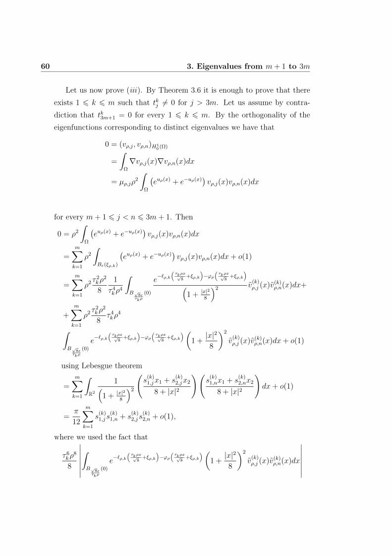
60 3. Eigenvalues from m+ 1 to 3m
Let us now prove (iii). By Theorem 3.6 it is enough to prove that there
exists 1 6 k 6 m such that tkj 6= 0 for j > 3m. Let us assume by contra-
diction that tk3m+1 = 0 for every 1 6 k 6 m. By the orthogonality of the
eigenfunctions corresponding to distinct eigenvalues we have that
0 = (vρ,j, vρ,n)H10 (Ω)
=
∫Ω
∇vρ,j(x)∇vρ,n(x)dx
= µρ,jρ2
∫Ω
(euρ(x) + e−uρ(x)
)vρ,j(x)vρ,n(x)dx
for every m+ 1 6 j < n 6 3m+ 1. Then
0 = ρ2
∫Ω
(euρ(x) + e−uρ(x)
)vρ,j(x)vρ,n(x)dx
=m∑k=1
ρ2
∫Bε(ξρ,k)
(euρ(x) + e−uρ(x)
)vρ,j(x)vρ,n(x)dx+ o(1)
=m∑k=1
ρ2 τ2kρ
2
8
1
τ 4kρ
4
∫B√8ετkρ
(0)
e−`ρ,k
(τkρx√
8+ξρ,k
)−ϕρ
(τkρx√
8+ξρ,k
)(
1 + |x|28
)2 v(k)ρ,j (x)v(k)
ρ,n(x)dx+
+m∑k=1
ρ2 τ2kρ
2
8τ 4kρ
4
∫B√8ετkρ
(0)
e−`ρ,k
(τkρx√
8+ξρ,k
)−ϕρ
(τkρx√
8+ξρ,k
)(1 +|x|2
8
)2
v(k)ρ,j (x)v(k)
ρ,n(x)dx+ o(1)
using Lebesgue theorem
=m∑k=1
∫R2
1(1 + |x|2
8
)2
(s
(k)1,jx1 + s
(k)2,jx2
8 + |x|2
)(s
(k)1,nx1 + s
(k)2,nx2
8 + |x|2
)dx+ o(1)
=π
12
m∑k=1
s(k)1,j s
(k)1,n + s
(k)2,j s
(k)2,n + o(1),
where we used the fact that
τ 6kρ
8
8
∣∣∣∣∣∣∣∫B√8ετkρ
(0)
e−`ρ,k
(τkρx√
8+ξρ,k
)−ϕρ
(τkρx√
8+ξρ,k
)(1 +|x|2
8
)2
v(k)ρ,j (x)v(k)
ρ,n(x)dx
∣∣∣∣∣∣∣

61
6 Cρ8 1
ρ6.
Then, having set sj = (s11,j, . . . , s
m1,j, s
12,j, . . . , s
m2,j) ∈ R2m, we get
m∑k=1
s(k)1,j s
(k)1,3m+1 + s
(k)2,j s
(k)2,3m+1 = sj · s3m+1 = 0; ∀m 6 j 6 3m,
but in R2m there are at most 2m orthogonal vectors, so that the condition
cannot be satisfied, from which we get a contradiction.

Chapter 4
Morse Index Computations
In this chapter, we will give an asymptotic estimate for the eigenvalues
and the eigenfunctions from m + 1 to 3m. While computing this estimate,
we will also calculate the Morse index.
Let us firstly prove the following lemma.
Lemma 4.1. If j is such that µρ,j → 1 and tj = 0, then for every k =
1, . . . ,m, we have
Λj,kρ := ρ2
∫Bε(ξρ,k)
(euρ(x) + e−uρ(x)
)vρ,j(x)dx = o(ρ).
Proof. By (3.2), for every j we have that
vρ,j(x) = µρ,j
m∑k=1
G(x, ξk)ρ2
∫Bε(ξρ,k)
(euρ(x) + e−uρ(x)
)vρ,j(x)dx+ o(1)
= µρ,j
m∑k=1
G(x, ξk)Λk,jρ + o(1)
in C1(Ω \ ξ1, . . . , ξm). Moreover, by Lemma 3.7 we have that
(1− µρ,j)ρ2
∫Bε(ξk)
(euρ(x) + e−uρ(x)
) ∂uρ∂xi
(x)vρ,j(x)dx
=
∫∂Bε(ξk)
(∂vρ,j∂ν
(x)∂uρ∂xi
(x)− vρ,j(x)∂2uρ∂ν∂xi
(x)
)dσx.
62

63
Let us start by studying the left hand side.
ρ2
∫Bε(ξk)
(euρ(x) + e−uρ(x)
) ∂uρ∂xi
(x)vρ,j(x)dx
= ρ2 τ2kρ
2
8
1
τ 4kρ
4
∫B√8ετkρ
(0)
e`ρ,k
(τkρx√
8+ξρ,k
)+ϕρ
(τkρx√
8+ξρ,k
)(
1 + |x|28
)2 v(k)ρ,j (x)
(− 4αk√
8τkρ
xi
1 + |x|28
+∂`ρ,k∂xi
(τkρx√
8+ ξρ,k
)+∂ϕρ∂xi
(τkρx√
8+ ξρ,k
))dx+
+ ρ2 τ2kρ
2
8τ 4kρ
4
∫B√8ετkρ
(0)
e−`ρ,k
(τkρx√
8+ξρ,k
)−ϕρ
(τkρx√
8+ξρ,k
)(1 +|x|2
8
)2
v(k)ρ,j (x)
(− 4αk√
8τkρ
xi
1 + |x|28
+∂`ρ,k∂xi
(τkρx√
8+ ξρ,k
)+∂ϕρ∂xi
(τkρx√
8+ ξρ,k
))dx+ o(1)
using Lebesgue theorem
= − 4√8ρ
αkτk
∫R2
xi(1 + |x|2
8
)3
(s
(k)1,jx1 + s
(k)2,jx2
8 + |x|2
)dx(1 + o(1))
= − 16
3√
8ρπαkτks
(k)i,j (1 + o(1)),
(4.1)
where we used the fact that
τ 6kρ
8
8
∣∣∣ ∫B√8ετkρ
(0)
e−`ρ,k
(τkρx√
8+ξρ,k
)−ϕρ
(τkρx√
8+ξρ,k
)(1 +|x|2
8
)2
v(k)ρ,j (x)
(− 4αk√
8τkρ
xi8 + |x|2
+∂`ρ,k∂xi
(τkρx√
8+ ξρ,k
))dx∣∣∣
6 Cρ8 1
ρ6
= o(1),
and∣∣∣∣∣∣∣∫B√8ετkρ
(0)
e`ρ,k
(τkρx√
8+ξρ,k
)+ϕρ
(τkρx√
8+ξρ,k
)(
1 + |x|28
)2 v(k)ρ,j (x)
∂ϕρ∂xi
(τkρx√
8+ ξρ,k
)dx
∣∣∣∣∣∣∣
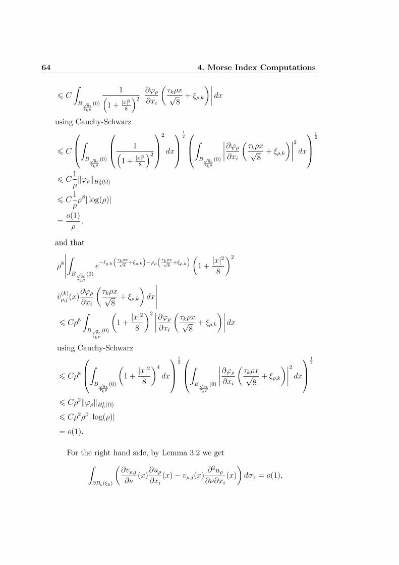
64 4. Morse Index Computations
6 C
∫B√8ετkρ
(0)
1(1 + |x|2
8
)2
∣∣∣∣∂ϕρ∂xi
(τkρx√
8+ ξρ,k
)∣∣∣∣ dxusing Cauchy-Schwarz
6 C
∫B√8ετkρ
(0)
1(1 + |x|2
8
)2
2
dx
12∫
B√8ετkρ
(0)
∣∣∣∣∂ϕρ∂xi
(τkρx√
8+ ξρ,k
)∣∣∣∣2 dx
12
6 C1
ρ‖ϕρ‖H1
0 (Ω)
6 C1
ρρβ| log(ρ)|
=o(1)
ρ,
and that
ρ8
∣∣∣∣∣∫B√8ετkρ
(0)
e−`ρ,k
(τkρx√
8+ξρ,k
)−ϕρ
(τkρx√
8+ξρ,k
)(1 +|x|2
8
)2
v(k)ρ,j (x)
∂ϕρ∂xi
(τkρx√
8+ ξρ,k
)dx
∣∣∣∣∣6 Cρ8
∫B√8ετkρ
(0)
(1 +|x|2
8
)2 ∣∣∣∣∂ϕρ∂xi
(τkρx√
8+ ξρ,k
)∣∣∣∣ dxusing Cauchy-Schwarz
6 Cρ8
∫B√8ετkρ
(0)
(1 +|x|2
8
)4
dx
12∫
B√8ετkρ
(0)
∣∣∣∣∂ϕρ∂xi
(τkρx√
8+ ξρ,k
)∣∣∣∣2 dx
12
6 Cρ2‖ϕρ‖H10 (Ω)
6 Cρ2ρβ| log(ρ)|
= o(1).
For the right hand side, by Lemma 3.2 we get∫∂Bε(ξk)
(∂vρ,j∂ν
(x)∂uρ∂xi
(x)− vρ,j(x)∂2uρ∂ν∂xi
(x)
)dσx = o(1),

65
hence
− 16
3√
8ρπαkτks
(k)i,j (1 + o(1))(1− µρ,j) = o(1),
and so
(1− µρ,j) = o(ρ).
By 3.4, and proceeding as in Theorem 3.6, we get
R
∫∂BR(ξk)
(2∂uρ∂ν
(x)∂vρ,j∂ν
(x)−∇uρ(x) · ∇vρ,j(x)
)dσ(x)
=
∫BR(ξk)
[(x− ξk) · ∇uρ(x)] ∆vρ,j(x) + [(x− ξk) · ∇vρ,j(x)] ∆uρ(x) dx
= −ρ2
∫∂BR(ξk)
(x− ξk) · ν(euρ(x) − e−uρ(x)
)vρ,j(x)dσ(x)+
+ 2ρ2
∫BR(ξk)
(euρ(x) − e−uρ(x)
)vρ,j(x)dx+
+ (1− µρ,j)ρ2
∫BR(ξk)
[(x− ξk) · ∇uρ(x)](euρ(x) + e−uρ(x)
)vρ,j(x)dx.
For the left hand side we have
R
∫∂BR(ξk)
(2∂uρ∂ν
(x)∂vρ,j∂ν
(x)−∇uρ(x) · ∇vρ,j(x)
)dσ(x)
= R
∫∂BR(ξk)
[2∂
∂ν
(8π
m∑i=1
G(x, ξi) + o(1)
)∂
∂ν
(µρ,j
m∑i=1
G(x, ξi)Λi,jρ + o(1)
)+
−∇
(8π
m∑i=1
G(x, ξi) + o(1)
)· ∇
(µρ,j
m∑i=1
G(x, ξi)Λi,jρ + o(1)
)]dσ(x)
using Lemma 3.5
= 4µρ,jΛk,jρ + oR(1).
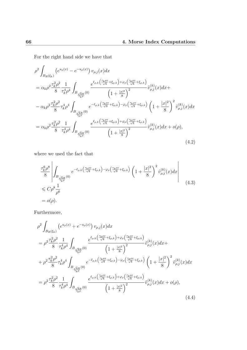
66 4. Morse Index Computations
For the right hand side we have that
ρ2
∫BR(ξk)
(euρ(x) − e−uρ(x)
)vρ,j(x)dx
= αkρ2 τ
2kρ
2
8
1
τ 4kρ
4
∫B√8Rτkρ
(0)
e`ρ,k
(τkρx√
8+ξρ,k
)+ϕρ
(τkρx√
8+ξρ,k
)(
1 + |x|28
)2 v(k)ρ,j (x)dx+
− αkρ2 τ2kρ
2
8τ 4kρ
4
∫B√8Rτkρ
(0)
e−`ρ,k
(τkρx√
8+ξρ,k
)−ϕρ
(τkρx√
8+ξρ,k
)(1 +|x|2
8
)2
v(k)ρ,j (x)dx
= αkρ2 τ
2kρ
2
8
1
τ 4kρ
4
∫B√8Rτkρ
(0)
e`ρ,k
(τkρx√
8+ξρ,k
)+ϕρ
(τkρx√
8+ξρ,k
)(
1 + |x|28
)2 v(k)ρ,j (x)dx+ o(ρ),
(4.2)
where we used the fact that
τ 6kρ
8
8
∣∣∣∣∣∣∣∫B√8Rτkρ
(0)
e−`ρ,k
(τkρx√
8+ξρ,k
)−ϕρ
(τkρx√
8+ξρ,k
)(1 +|x|2
8
)2
v(k)ρ,j (x)dx
∣∣∣∣∣∣∣6 Cρ8 1
ρ6
= o(ρ).
(4.3)
Furthermore,
ρ2
∫BR(ξk)
(euρ(x) + e−uρ(x)
)vρ,j(x)dx
= ρ2 τ2kρ
2
8
1
τ 4kρ
4
∫B√8Rτkρ
(0)
e`ρ,k
(τkρx√
8+ξρ,k
)+ϕρ
(τkρx√
8+ξρ,k
)(
1 + |x|28
)2 v(k)ρ,j (x)dx+
+ ρ2 τ2kρ
2
8τ 4kρ
4
∫B√8Rτkρ
(0)
e−`ρ,k
(τkρx√
8+ξρ,k
)−ϕρ
(τkρx√
8+ξρ,k
)(1 +|x|2
8
)2
v(k)ρ,j (x)dx
= ρ2 τ2kρ
2
8
1
τ 4kρ
4
∫B√8Rτkρ
(0)
e`ρ,k
(τkρx√
8+ξρ,k
)+ϕρ
(τkρx√
8+ξρ,k
)(
1 + |x|28
)2 v(k)ρ,j (x)dx+ o(ρ),
(4.4)
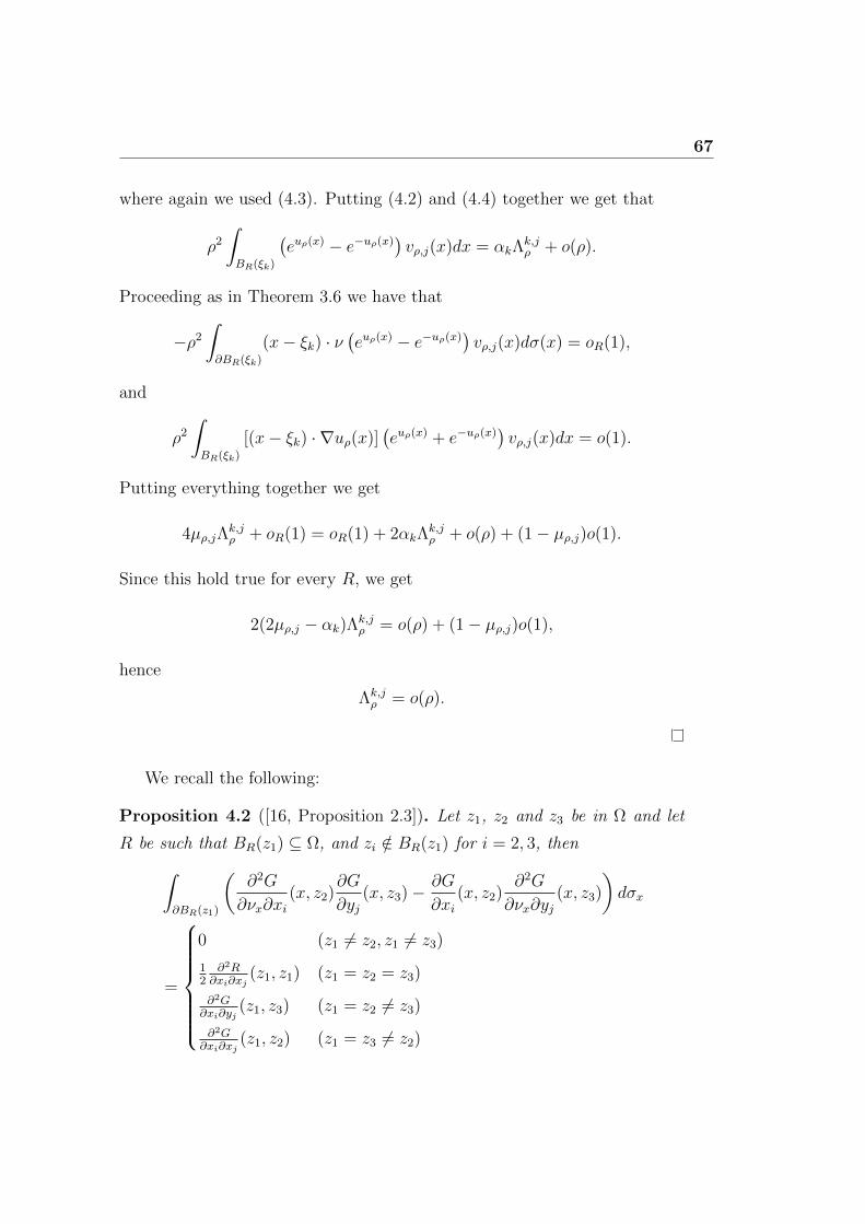
67
where again we used (4.3). Putting (4.2) and (4.4) together we get that
ρ2
∫BR(ξk)
(euρ(x) − e−uρ(x)
)vρ,j(x)dx = αkΛ
k,jρ + o(ρ).
Proceeding as in Theorem 3.6 we have that
−ρ2
∫∂BR(ξk)
(x− ξk) · ν(euρ(x) − e−uρ(x)
)vρ,j(x)dσ(x) = oR(1),
and
ρ2
∫BR(ξk)
[(x− ξk) · ∇uρ(x)](euρ(x) + e−uρ(x)
)vρ,j(x)dx = o(1).
Putting everything together we get
4µρ,jΛk,jρ + oR(1) = oR(1) + 2αkΛ
k,jρ + o(ρ) + (1− µρ,j)o(1).
Since this hold true for every R, we get
2(2µρ,j − αk)Λk,jρ = o(ρ) + (1− µρ,j)o(1),
hence
Λk,jρ = o(ρ).
We recall the following:
Proposition 4.2 ([16, Proposition 2.3]). Let z1, z2 and z3 be in Ω and let
R be such that BR(z1) ⊆ Ω, and zi /∈ BR(z1) for i = 2, 3, then∫∂BR(z1)
(∂2G
∂νx∂xi(x, z2)
∂G
∂yj(x, z3)− ∂G
∂xi(x, z2)
∂2G
∂νx∂yj(x, z3)
)dσx
=
0 (z1 6= z2, z1 6= z3)
12
∂2R∂xi∂xj
(z1, z1) (z1 = z2 = z3)
∂2G∂xi∂yj
(z1, z3) (z1 = z2 6= z3)
∂2G∂xi∂xj
(z1, z2) (z1 = z3 6= z2)
68 4. Morse Index Computations
We will now give an estimate for the eigenfunctions away from the blow-
up points. This estimate will hold precisely when the one provided by Lemma
3.3 doesn’t hold, that is for the eigenfunctions from m+ 1 to 3m. Moreover,
we will identify the connection between the Morse index of uρ and that of
the Hamilton function F .
Proposition 4.3. Let j be such that tj = 0. Then
vρ,jρ→ 2π
m∑k=1
τk√8
(s
(k)1,j
∂G
∂x1
(x, ξk) + s(k)2,j
∂G
∂x2
(x, ξk)
)(4.5)
in C1loc(Ω \ ξ1, . . . , ξm). Furthermore
(1− µρ,n) = 3πρ2ηn(1 + o(1)), (4.6)
where the ηn’s, for n = 1, . . . , 2m, are the eigenvalues of the matrix D(HessF)D,
where D is the diagonal matrix D = diag(τ1, . . . , τm, τ1, . . . , τm), and HessFis the Hessian matrix of the Hamilton function F .
Proof. Let K ⊆ Ω \ ξ1, . . . , ξm be compact. Let
ε′ = mink
infρ
dist(K, ξρ,k),
and let λ = min(ε, ε′). Since G(·, ·) is smooth on K × Bλ(ξρ,k), we can
consider its Taylor expansion to get
G(x, y) = G(x, ξρ,k) +∑i=1,2
∂G
∂yi(x, ξρ,k)(y − ξρ,k)i+
+1
2
∑i,h=1,2
∂2G
∂yi∂yh(x, ηρ)(y − ξρ,k)i(y − ξρ,k)h,
where ηρ is a point lying on the segment connecting y to ξρ,k, and hence
contained in Bλ(ξρ,k). Taking λ = ργ with γ < 14
we get∣∣∣∣∣µρ,jρ2
∫Ω\∪mk=1Bλ(ξρ,k)
(euρ(y) + e−uρ(y)
)vρ,j(y)G(x, y)dy
∣∣∣∣∣6 C
(ρ2
(ρ2 + λ2)2 + ρ2
)∫Ω\∪mk=1Bλ(ξρ,k)
|G(x, y)|dy

69
since G(x, ·) ∈ L1(Ω)
= o(ρ).
Using Green’s representation formula, for each x ∈ K, we have
vρ,j(x) = µρ,jρ2
∫Ω
(euρ(y) + e−uρ(y)
)vρ,j(y)G(x, y)dy
= µρ,j
m∑k=1
ρ2
∫Bλ(ξρ,k)
(euρ(y) + e−uρ(y)
)vρ,j(y)G(x, y)dy+
+ µρ,jρ2
∫Ω\∪mk=1Bλ(ξρ,k)
(euρ(y) + e−uρ(y)
)vρ,j(y)G(x, y)dy
= µρ,j
m∑k=1
ρ2
∫Bλ(ξρ,k)
(euρ(y) + e−uρ(y)
)vρ,j(y)(
G(x, ξρ,k) +∑i=1,2
∂G
∂yi(x, ξρ,k)(y − ξρ,k)i
)dy+
+µρ,j2
m∑k=1
ρ2
∫Bλ(ξρ,k)
(euρ(y) + e−uρ(y)
)vρ,j(y)
∑i,h=1,2
∂2G
∂yi∂yh(x, ηρ)(y − ξρ,k)i(y − ξρ,k)hdy + o(ρ)
= µρ,j
m∑k=1
ρ2
∫Bλ(ξρ,k)
(euρ(y) + e−uρ(y)
)vρ,j(y)(
G(x, ξρ,k) +∑i=1,2
∂G
∂yi(x, ξρ,k)(y − ξρ,k)i
)dy +Rρ + o(ρ),
having set
Rρ =µρ,j2
m∑k=1
ρ2
∫Bλ(ξρ,k)
(euρ(y) + e−uρ(y)
)vρ,j(y)
∑i,h=1,2
∂2G
∂yi∂yh(x, ηρ)(y − ξρ,k)i(y − ξρ,k)hdy.
Since ηρ ∈ Bλ(ξρ,k) and x /∈ Bλ(ξρ,k), we have∣∣∣∣ ∂2G
∂yi∂yh(x, ηρ)
∣∣∣∣ 6 supi,h=1,2;z∈Bλ(ξρ,k)
∣∣∣∣ ∂2G
∂yi∂yh(x, z)
∣∣∣∣ 6 C.
70 4. Morse Index Computations
Since µρ,j = 1 + o(1), we have
|Rρ| 6 C
m∑k=1
ρ2
∫Bλ(ξρ,k)
(euρ(y) + e−uρ(y)
)|y − ξρ,k|2dy
= Cm∑k=1
ρ2 τ2kρ
2
8
1
τ 4kρ
4
τ 2kρ
2
8
∫B√8λτkρ
(0)
e`ρ,k
(τkρy√
8+ξρ,k
)+ϕρ
(τkρy√
8+ξρ,k
)(
1 + |y|28
)2 |y|2dy+
+ Cm∑k=1
ρ2 τ2kρ
2
8τ 4kρ
4 τ2kρ
2
8∫B√8λτkρ
(0)
e−`ρ,k
(τkρy√
8+ξρ,k
)−ϕρ
(τkρy√
8+ξρ,k
)(1 +|y|2
8
)2
|y|2dy
= o(ρ),
where we used the fact that
ρ2
∣∣∣∣∣∣∣∫B√8λτkρ
(0)
e`ρ,k
(τkρy√
8+ξρ,k
)+ϕρ
(τkρy√
8+ξρ,k
)(
1 + |y|28
)2 |y|2dy
∣∣∣∣∣∣∣6 Cρ2
∫B√8λτkρ
(0)
|y|2(1 + |y|2
8
)2dy
6 Cρ2 (log(ρ) + 1)
= o(ρ)
and
ρ10
∣∣∣∣∣∣∣∫B√8λτkρ
(0)
e−`ρ,k
(τkρy√
8+ξρ,k
)−ϕρ
(τkρy√
8+ξρ,k
)(1 +|y|2
8
)2
|y|2dy
∣∣∣∣∣∣∣6 Cρ10 1
ρ8
= o(ρ).
Therefore
vρ,j(x) = µρ,j
m∑k=1
ρ2
∫Bλ(ξρ,k)
(euρ(y) + e−uρ(y)
)vρ,j(y)G(x, ξρ,k)dy+

71
+ µρ,j
m∑k=1
ρ2
∫Bλ(ξρ,k)
(euρ(y) + e−uρ(y)
)vρ,j(y)
∑i=1,2
∂G
∂yi(x, ξρ,k)(y − ξρ,k)idy + o(ρ)
= µρ,j
m∑k=1
(G(x, ξk) + o(1)) ρ2
∫Bλ(ξρ,k)
(euρ(y) + e−uρ(y)
)vρ,j(y)dy+
+ µρ,j∑i=1,2
∂G
∂yi(x, ξk) (1 + o(1))
m∑k=1
ρ2
∫Bλ(ξρ,k)
(euρ(y) + e−uρ(y)
)vρ,j(y)(y − ξρ,k)idy + o(ρ)
using Lemma 4.1
= µρ,j∑i=1,2
∂G
∂yi(x, ξk) (1 + o(1))
m∑k=1
ρ2 τ2kρ
2
8
1
τ 4kρ
4
τkρ
8
∫B√8λτkρ
(0)
e`ρ,k
(τkρy√
8+ξρ,k
)+ϕρ
(τkρy√
8+ξρ,k
)(
1 + |y|28
)2 v(k)ρ,j (y)yidy+
+ µρ,j∑i=1,2
∂G
∂yi(x, ξk) (1 + o(1))
m∑k=1
ρ2 τ2kρ
2
8τ 4kρ
4 τkρ
8∫B√8λτkρ
(0)
e−`ρ,k
(τkρy√
8+ξρ,k
)−ϕρ
(τkρy√
8+ξρ,k
)(1 +|y|2
8
)2
v(k)ρ,j (y)yidy + o(ρ)
= µρ,j∑i=1,2
∂G
∂yi(x, ξk)(1 + o(1))
m∑k=1
1
8τ 2k
τkρ√8
∫B√8λτkρ
(0)
e`ρ,k
(τkρy√
8+ξρ,k
)+ϕρ
(τkρy√
8+ξρ,k
)(
1 + |y|28
)2 v(k)ρ,j (y)yidy + o(ρ),
since
ρ9
∣∣∣∣∣∣∣∫B√8λτkρ
(0)
e−`ρ,k
(τkρy√
8+ξρ,k
)−ϕρ
(τkρy√
8+ξρ,k
)(1 +|y|2
8
)2
v(k)ρ,j (y)yidy
∣∣∣∣∣∣∣

72 4. Morse Index Computations
6 Cρ9 1
ρ7
= o(ρ).
Therefore
vρ,j(x)
ρ= µρ,j
∑i=1,2
∂G
∂yi(x, ξk)(1 + o(1))
m∑k=1
1
8τ 2k
τk√8
∫B√8λτkρ
(0)
e`ρ,k
(τkρy√
8+ξρ,k
)+ϕρ
(τkρy√
8+ξρ,k
)(
1 + |y|28
)2 v(k)ρ,j (y)yidy + o(1)
using Lebesgue
= µρ,j∑i=1,2
∂G
∂yi(x, ξk)(1 + o(1))
m∑k=1
τk√8∫
R2
yi(1 + |y|2
8
)2
s(k)1,jy1 + s
(k)2,jy2
8 + |y|2dy + o(1)
= 2πµρ,j∑i=1,2
m∑k=1
∂G
∂yi(x, ξk)
τks(k)i,j√8
+ o(1),
and so 4.5 is proved.
By Lemma 3.7, we get
(1− µρ,n)ρ2
∫Bε(ξk)
(euρ(x) + e−uρ(x)
) ∂uρ∂xj
(x)vρ,n(x)dx
=
∫∂Bε(ξk)
(∂vρ,n∂ν
(x)∂uρ∂xj
(x)− vρ,n(x)∂2uρ∂ν∂xj
(x)
)dσx.
For the left hand side, using (4.1), we have
ρ2
∫Bε(ξρ,k)
(euρ(x) + e−uρ(x)
) ∂uρ∂xj
(x)vρ,n(x)dx+o(1) = − 16
3√
8ρπαkτks
(k)j,n(1+o(1)).
For the right hand side we have∫∂Bε(ξk)
(∂vρ,n∂ν
(x)∂uρ∂xj
(x)− vρ,n(x)∂2uρ∂ν∂xj
(x)
)dσx
= ρ
∫∂Bε(ξk)
∂
∂νx
(2πµρ,n
∑i=1,2
m∑l=1
∂G
∂yi(x, ξl)
τls(l)i,n√8
+ o(1)
)

73
∂
∂xj
(8π
m∑h=1
αhG(x, ξh) + o(1)
)dσx+
− ρ∫∂Bε(ξk)
(2πµρ,n
∑i=1,2
m∑l=1
∂G
∂yi(x, ξl)
τls(l)i,n√8
+ o(1)
)∂2
∂xj∂νx
(8π
m∑h=1
αhG(x, ξh) + o(1)
)dσx
= 16π2ρµρ,n
m∑l,h=1
∑i=1,2
αhτls
(l)i,n√8∫
∂Bε(ξk)
(∂2G
∂yi∂νx(x, ξl)
∂G
∂xj(x, ξh)−
∂G
∂yi(x, ξl)
∂2G
∂xj∂νx(x, ξh)
)dσx + o(ρ)
using Proposition 4.2
= −16π2αkρµρ,n
m∑l=1
∑i=1,2
τls(l)i,n√8
∂2F∂x
(l)i ∂x
(k)j
(ξ1, . . . , ξm) + o(ρ),
Hence
− 16
3√
8ρπαkτks
(k)j,n(1 + o(1))(1− µρ,n)
= −16π2αkρµρ,n
m∑l=1
∑i=1,2
τls(l)i,n√8
∂2F∂x
(l)i ∂x
(k)j
(ξ1, . . . , ξm) + o(ρ).
Having set
ηn :=
∑ml=1
∑i=1,2 τlτks
(l)i,n
∂2F∂x
(l)i ∂x
(k)j
(ξ1, . . . , ξm)
s(k)j,n
,
we get
s(k)j,nηn =
m∑l=1
∑i=1,2
τlτks(l)i,n
∂2F∂x
(l)i ∂x
(k)j
(ξ1, . . . , ξm),
so that sn =(s
(1)1,n, . . . , s
(m)1,n , s
(1)2,n, . . . , s
(m)2,n
)and ηn are respectively the eigen-
functions and the eigenvalues of the matrix D(HessF)D. We can therefore
conclude that
(1− µρ,n) = 3πρ2ηn + o(ρ2).

74 4. Morse Index Computations
Finally, we can prove the following.
Proof of Theorem 0.2. .
Proposition 4.3 proves point 1 and point 3, while Theorem 3.6 jointly
with point (i) of Proposition 3.9 proves point 2.
And
Proof of Theorem 0.3. .
With similar calculus of those in Proposition 3.9 we can prove that for
3m + 1 < j 6 4m, µρ,j still goes to one. In the proof of point (iii) in
Proposition 3.9 we showed that for 3m+ 1 < j 6 4m, t(k)j 6= 0, so Lemma 3.3
holds and in such a case at the end of Theorem 3.6 we proved (3.8), therefore
point 1 and point 3 are proved. Finally, considering Proposition 3.1 and the
fact that the functions 8−|x|28+|x|2 and xi
8+|x|2 , for i = 1, 2, are orthogonal and that
eigenfunctions relative to different eigenspaces have to be orthogonal we get
point 2.
We are now ready to prove the main result.
Proof of Theorem 0.4. .
For ρ sufficiently small, by Proposition 2.3 we have that µρ,j < 1 for every
j = 1, . . . ,m. By Proposition 3.9 we have that µρ,j > 1 for j > 3m and for
every m + 1 6 j 6 3m we have that µρ,j 6 1 + Cρ2, so by Theorem 3.6 we
get tj = 0. Therefore, since the hypotheses of Proposition 4.3 are satisfied,
we get
µρ,j = 1− 3πρ2ηj(1 + o(1)),
where the ηj’s, for j = 1, . . . , 2m, are the eigenvalues of the matrix
D(HessF)D. Then, to any positive eigenvalue ηj of the matrix D(HessF)D
there corresponds a negative µρ,j. Since D is a diagonal, positive definite
matrix, the signature of the matrix D(HessF)D is equal to the signature of
the matrix HessF , and hence the theorem is proved.
We deduce the following corollary.

75
Proof of Corollary 0.5. .
It is enough to notice that HessF is a 2m × 2m matrix, and so 0 6
M(HessF) 6 2m.

Bibliography
[1] Daniele Bartolucci and Angela Pistoia. Existence and qualitative prop-
erties of concentrating solutions for the sinh-Poisson equation. IMA J.
Appl. Math., 72(6):706–729, 2007.
[2] Thomas Bartsch, K-C Chang, and Z-Q Wang. On the morse indices of
sign changing solutions of nonlinear elliptic problems. Mathematische
Zeitschrift, 233(4):655–677, 2000.
[3] Thomas Bartsch, Angela Pistoia, and Tobias Weth. N-vortex equilibria
for ideal fluids in bounded planar domains and new nodal solutions of
the sinh-poisson and the lane-emden-fowler equations. Communications
in Mathematical Physics, 297(3):653–686, 2010.
[4] Emanuele Caglioti, Pierre-Louis Lions, Carlo Marchioro, and M Pul-
virenti. A special class of stationary flows for two-dimensional Euler
equations: a statistical mechanics description. Part II. Communications
in Mathematical Physics, 174(2):229–260, 1995.
[5] Emanuele Caglioti, Pierre-Louis Lions, Carlo Marchioro, and Mario
Pulvirenti. A special class of stationary flows for two-dimensional Eu-
ler equations: a statistical mechanics description. Communications in
Mathematical physics, 143(3):501–525, 1992.
[6] Alexandre J Chorin. Vorticity and turbulence, volume 103. Springer
Science & Business Media, 2013.
76
BIBLIOGRAPHY 77
[7] Alexandre Joel Chorin, Jerrold E Marsden, and Jerrold E Marsden. A
mathematical introduction to fluid mechanics, volume 3. Springer, 1990.
[8] KW Chow, NWM Ko, RCK Leung, and SK Tang. Inviscid two di-
mensional vortex dynamics and a soliton expansion of the sinh-Poisson
equation. Physics of fluids, 10(5):1111–1119, 1998.
[9] KW Chow, SC Tsang, and CC Mak. Another exact solution for two-
dimensional, inviscid sinh Poisson vortex arrays. Physics of Fluids,
15(8):2437–2440, 2003.
[10] Thierry Dauxois, Stephan Fauve, and Laurette Tuckerman. Stability of
periodic arrays of vortices. Physics of Fluids, 8(2):487–495, 1996.
[11] Francesca De Marchis, Isabella Ianni, and Filomena Pacella. Exact
Morse index computation for nodal radial solutions of Lane–Emden
problems. Mathematische Annalen, 367(1-2):185–227, 2017.
[12] Khalil El Mehdi and Massimo Grossi. Asymptotic estimates and qual-
itative properties of an elliptic problem in dimension two. Advanced
Nonlinear Studies, 4(1):15–36, 2004.
[13] Pierpaolo Esposito, Massimo Grossi, and Angela Pistoia. On the exis-
tence of blowing-up solutions for a mean field equation. In Annales de
l’IHP Analyse non lineaire, volume 22, pages 227–257, 2005.
[14] Francesca Gladiali and Massimo Grossi. On the spectrum of a nonlinear
planar problem. Ann. Inst. H. Poincare Anal. Non Lineaire, 26(1):191–
222, 2009.
[15] Francesca Gladiali, Massimo Grossi, Hiroshi Ohtsuka, and Takashi
Suzuki. Morse indices of multiple blow-up solutions to the two-
dimensional Gel’fand problem. Comm. Partial Differential Equations,
39(11):2028–2063, 2014.

78 BIBLIOGRAPHY
[16] Massimo Grossi, Hiroshi Ohtsuka, Takashi Suzuki, et al. Asymptotic
non-degeneracy of the multiple blow-up solutions to the Gel’fand prob-
lem in two space dimensions. Adv. Differential Equations, 16(1/2):145–
164, 2011.
[17] Massimo Grossi and Angela Pistoia. Multiple blow-up phenomena for
the sinh-poisson equation. Archive for Rational Mechanics and Analysis,
209(1):287–320, 2013.
[18] D Gurarie and KW Chow. Vortex arrays for sinh-Poisson equation
of two-dimensional fluids: Equilibria and stability. Physics of Fluids,
16(9):3296–3305, 2004.
[19] Glenn Joyce and David Montgomery. Negative temperature states for
the two-dimensional guiding-centre plasma. Journal of Plasma Physics,
10(1):107–121, 1973.
[20] S Julien, J-M Chomaz, and J-C Lasheras. Three-dimensional stabil-
ity of periodic arrays of counter-rotating vortices. Physics of Fluids,
14(2):732–743, 2002.
[21] Gustav Robert Kirchhoff. Vorlesungen uber mathematische physik:
mechanik, volume 1. Teubner, 1876.
[22] Andrew J Majda and Margaret Holen. Dissipation, topography, and
statistical theories for large-scale coherent structure. Communications
on Pure and Applied Mathematics: A Journal Issued by the Courant
Institute of Mathematical Sciences, 50(12):1183–1234, 1997.
[23] R Mallier and SA Maslowe. A row of counter-rotating vortices. Physics
of Fluids A: Fluid Dynamics, 5(4):1074–1075, 1993.
[24] Carlo Marchioro and Mario Pulvirenti. Mathematical theory of incom-
pressible nonviscous fluids, volume 96. Springer Science & Business
Media, 2012.

BIBLIOGRAPHY 79
[25] WH Matthaeus, WT Stribling, D Martinez, S Oughton, and D Mont-
gomery. Decaying, two-dimensional, Navier-Stokes turbulence at very
long times. Physica D: Nonlinear Phenomena, 51(1-3):531–538, 1991.
[26] William H Matthaeus, W Troy Stribling, Daniel Martinez, Sean
Oughton, and David Montgomery. Selective decay and coherent vortices
in two-dimensional incompressible turbulence. Physical review letters,
66(21):2731–2734, 1991.
[27] John Milnor. Morse theory.(AM-51), volume 51. Princeton university
press, 2016.
[28] David Montgomery and Glenn Joyce. Statistical mechanics of “negative
temperature” states. The Physics of Fluids, 17(6):1139–1145, 1974.
[29] David Montgomery, William H Matthaeus, WT Stribling, D Martinez,
and Sean Oughton. Relaxation in two dimensions and the “sinh-Poisson”
equation. Physics of Fluids A: Fluid Dynamics, 4(1):3–6, 1992.
[30] David Montgomery, William H Matthaeus, WT Stribling, D Martinez,
and Sean Oughton. Relaxation in two dimensions and the “sinh-
Poisson”equation. Physics of Fluids A: Fluid Dynamics, 4(1):3–6, 1992.
[31] Marston Morse. The calculus of variations in the large, volume 18.
American Mathematical Soc., 1934.
[32] Marston Morse and Stewart S Cairns. Critical point theory in global
analysis and differential topology: An introduction, volume 33. Academic
Press, 2014.
[33] Hiroshi Ohtsuka. To what extent can the Hamiltonian of vortices il-
lustrate the mean field of equilibrium vortices? (Modern approach
and developments to Onsager’s theory on statistical vortices). RIMS
Kokyuroku Bessatsu, 1798:1–17, 2012.
80 BIBLIOGRAPHY
[34] DA Schecter, DHE Dubin, KS Fine, and CF Driscoll. Vortex crystals
from 2D Euler flow: Experiment and simulation. Physics of Fluids,
11(4):905–914, 1999.
[35] F Spineanu and M Vlad. Stationary vortical flows in two-dimensional
plasma and in planetary atmospheres. Physical review letters,
94(23):235003, 2005.
[36] Z Yin, DC Montgomery, and HJH Clercx. Alternative statistical-
mechanical descriptions of decaying two-dimensional turbulence in terms
of “patches” and “points”. Physics of Fluids, 15(7):1937–1953, 2003.