1

Development of an Improved Method for Estimating Fugitive PM10 Emissions from Windblown Dust from Agricultural Lands

Stephen R. Francis, Skip G. Campbell and Dale R. ShimpCalifornia Air Resources Board

2020 L StreetP.O. Box 2815

Sacramento, CA 95812-2815

ABSTRACT

The standard methodology for estimating agricultural windblown dust, referred to as the winderosion equation (WEQ), tends to produce inflated emission estimates for California. This occurs in partbecause it was developed in the Midwestern United States, and, therefore, does not take into accountmany of the environmental conditions and farm practices specific to California. The California AirResources Board (ARB) staff has modified the WEQ to improve the emission estimate. This revisionincludes improved climatic factors, adjustments for the long-term effects of irrigation (cloddiness), as wellas the short-term effects of irrigation on erodibility (surface wetness). Crop canopy coverage,postharvest soil cover, postharvest replanting to a different crop, as well as bare and border field regionsare also accounted for in this revision. The monthly emissions profile now reflects variations intemperature, precipitation, irrigation, canopy coverage, postharvest soil cover, postharvest replanting toanother crop, as well as wind. The result has been a downward revision in the annual emissions estimateof approximately 80 percent. The new annual and monthly emissions estimates better reflect the ambientmonitoring source apportionment results, as well as California crop production patterns and climaticconditions.

INTRODUCTION

California agricultural practices are different from much of the rest of the United States, andencourage approaches for estimating emissions that are in many respects quite different as well. California farmers grow a wide variety of crops, commonly irrigate, and, in most regions of the state,grow crops year-round. In addition, California exhibits subregional variations in climate due to terrain. In an effort to better reflect these attributes, the ARB staff has significantly modified the 1989 ARBagricultural windblown dust emissions methodology, referred to here as the ARBWEQ1, used first to 1

produce the inventory that was based on 1987 crop acreages.The standard methodology for estimating the emission factor for windblown emissions from

agricultural lands, which was used for the ARBWEQ1, is the wind erosion equation or WEQ. Thismethod produces an annual estimate of emissions, which can also be adjusted to estimate monthlyemissions. Since the implementation of the ARBWEQ1, the ARB staff has received many commentsquestioning the large windblown emission estimates it generates. In the case of California, the excessiveemissions estimated by the ARBWEQ1 are in part due to the fact that the WEQ is based on MidwesternUnited States agricultural conditions and practices. The WEQ was developed by the United StatesDepartment of Agriculture - Agricultural Research Service (USDA-ARS) during the 1960's, for theestimation of wind erosion on agricultural land. The United States Environmental Protection Agency2,3

(U.S. EPA) adapted the USDA-ARS methodology for use in estimating windblown particulate matter(PM) emissions from agricultural lands in 1974 (page 144 et seq. of EPA-450/3-74-037). The U.S.4

EPA methodology was then adapted by ARB staff for the ARBWEQ1.In the time since the ARBWEQ1 was produced, the USDA-ARS has been conducting ambitious

programs to replace the WEQ with improved wind erosion prediction models. These USDA-ARS

2

programs include the development of the Revised Wind Erosion Equation (RWEQ) and the Wind5

Erosion Prediction System (WEPS) models. To date, these models have not proven feasible for use by6

the ARB, although certain portions of the RWEQ have been incorporated into the ARB methodologywith this revision. This latest ARB methodology for estimating windblown agricultural emissions forparticulate matter less than ten microns in size (PM10), described in this paper, will be referred to here asthe ARBWEQ2.

METHODOLOGY

The calculations for the ARBWEQ2 are only summarized here. Additional background, anddetails on the methodology are included in the actual methodology document and the supplemental7

documentation to this methodology, which are available on request from the ARB. Among the8

refinements incorporated into the ARBWEQ2 are: Improved annual and monthly climatic factors,irrigation effects, crop canopy, soil cover, replanting (multiple crops within an annual cycle), andestimates of bare and border region effects.

The acreages of agricultural crops used in the ARBWEQ2 are from the 1993 harvested acreagedata provided to ARB staff by the California Department of Food and Agriculture (CDFA). The9

ARBWEQ2 has been applied to nearly all of the crops in the CDFA data base whose production might beexpected to result in windblown emissions. Pasture lands have been included for the first time with thisrevision. Orchard and vineyard acreages have been excluded, in part because it is postulated thatwindblown dust emissions from mature orchards will be relatively minor, and in part because themethodologies for determining the emissions have not been developed.

Creating the ARBWEQ2 from the WEQ

The agricultural land windblown dust emission estimate is obtained by multiplying the process rate(crop acreage) by an emission factor (tons of suspended PM10 per acre per year). On page 144 et seq.of the EPA-450/3-74-037 document the U.S. EPA established the following modification of the USDA-4

ARS WEQ:

E = AIKCL'V' S

whereE = emission factor: suspended particulate fraction of wind erosion losses of tilled fields, S

tons/acre/yearA = portion of total wind erosion losses that would be measured as suspended particulate,

estimated to be .025I = soil erodibility, tons/acre/yearK = surface roughness factor, dimensionlessC = annual climatic factor, dimensionlessL' = unsheltered field width factor, dimensionlessV' = vegetative cover factor, dimensionless

The soil erodibility (“I”) was initially established for the WEQ for a large, flat, bare field inKansas. Kansas has relatively high winds, along with hot summers, and low precipitation. The “K”, “C”,“L'” and “V'” factors serve to adjust the equation for applicability to field conditions that differ from theoriginal Kansas field. The overall approach to calculating emissions used in the WEQ was also used inthe ARBWEQ1. However, the WEQ monthly profile was based only on the monthly “C” factor, whilethe ARBWEQ1 profile was based loosely on statewide erosive energy estimates. The ARBWEQ2 bycontrast, while still retaining many of the factors present in the WEQ, is dramatically different in howsome of the factors are derived, and has replaced factors and added others, along with adopting a

3

temporal approach to the calculation that allows the emission estimate to include factors that change frommonth to month. The rest of this section summarizes the ARBWEQ2 implementation of the WEQ.

The “A” factor has been used in the ARBWEQ2 without modification. In the WEQ, “I” is afunction of soil particle diameter, which can be estimated for various soil textural classes from Table A-1of the above U.S. EPA methodology. For the ARBWEQ2 the soil textural classes were determined byARB staff from University of California soil maps. For most of the San Joaquin Valley Air Basin (SJV)10

counties an additional level of detail was included in the ARBWEQ2, by using the NRCS’ StateGeographic Data Base (STATSGO) of soil data. The ARBWEQ2 also added a USDA-ARS11

recommended adjustment for changes to long term erodibility due to irrigation. This affects a property12

known as cloddiness, and, in this case, refers to the increased tendency for a soil to form stableagglomerations after being exposed to irrigation water. The same USDA-ARS source also provided themethodology implemented in the ARBWEQ2 to estimate the short-term effects of irrigation on erodibilitydue to surface wetness.

The “K” factor reflects the reduction in wind erosion due to ridges, furrows, and soil clods. The“K” factor is crop specific. The ARBWEQ2 values for “K” were derived from Table A-2 in the aboveU.S. EPA methodology. The annual climatic factor “C” is based on data that show that erosion variesdirectly with the wind speed cubed, and as the inverse of the square of surface soil moisture. For theARBWEQ2, ARB staff improved the input data, as well as the methods associated with developing thecounty wide averaged annual climatic factor. Monthly climatic factors for the ARBWEQ2 were obtainedby modifying the annual “C” factor calculation method. Figure A-5 in the U.S. EPA methodology 4

allows the calculation of the unsheltered field width factor (“L'”) from the unsheltered field width (“L”)and the product of erodibility (“I”) and surface roughness (“K”). The values for “L” used in theARBWEQ2 were derived from Table A-2 in the above U.S. EPA methodology.

The vegetative cover factor “V'” is especially problematic for California, and was completelyreplaced by a series of factors in the ARBWEQ2 (see analysis below). The “V'” factor assumes a certaindegree of erosion reduction year round based upon postharvest vegetative debris. This factor does notaccount for barren fields from land preparation, growing canopy cover, or replanting of crops during asingle annual cycle. All of these factors are very important in the estimation of windblown agriculturaldust emissions in California. Therefore, ARB staff replaced the “V'” factor with separate crop canopycover and postharvest soil cover factors. Although the postharvest replant factor is listed in this report asa partial replacement for the “V'” factor, it actually affects the ARBWEQ2 calculation more broadly. Thepostharvest replant factor is implemented by removing the replanted acreage from the inventory at thetime of replanting. Therefore, all of the temporally calculated components will be affected by thisadjustment. There were no provisions in the WEQ to adjust for barren regions of planted fields, or fieldborder areas. Bare and border region adjustments have been included in the ARBWEQ2. The followingsections provide more detail on some of the more interesting methodology changes between the WEQ(ARBWEQ1) and the ARBWEQ2.

Because current environmental law focuses on PM10 rather than PM, the ARB used a conversionfactor of 0.5 in both the ARBWEQ1 and the ARBWEQ2 in order to estimate the PM10 emissionsfraction of the windblown agricultural PM emissions. This factor is consistent with studies of emissionsfrom soils in the SJV. 13

Climate-based Improvements in the ARBWEQ2

Annual “C” Factor

Page 154 of the EPA-450/3-74-037 document includes a definition of the “C” factor which4

agrees with the method utilized by the United States Department of Agriculture - Natural ResourcesConservation Service (NRCS). It incorporates the monthly precipitation effectiveness derived from14

precipitation and temperature, along with monthly average wind speeds. Garden City, Kansas is assigned

4

a factor of 1.0 and the “C” factors for all other sites are adjusted from this using the “C” factorcalculation. For the ARBWEQ1, ARB staff used NRCS-produced California statewide and county “C”factor contour maps. The data used for producing these contour maps came from a number of sources15

(see supplemental documentation for reference list). For the ARBWEQ2, the ARB staff produced8

contour maps using updated California Irrigation Management System (CIMIS) data, that were then16

grid counted to determine the weighted average “C” factors for the agricultural production land in eachcounty. The CIMIS data were collected using standard methodologies that more closely reflected theconditions encountered by agricultural fields than other climatic data sources.

Monthly “C” Factor

To account for California seasonality, ARB staff devised a method termed the “month-as-a-year”method which produced “C” factors which would apply if the climate for a given month were instead theyear round climate. Once normalized, these numbers provided the climate-based temporal profile.

The month-as-a-year method in the ARBWEQ2 produces pronounced curves with small “C”factors (resulting in lower emissions) in the cool, wet and more stagnant periods, and large “C” factors(and higher emissions) in the hot, dry, and windy periods. The method suggested by the U.S. EPA 4

substitutes monthly wind speed for annual wind speed, and yields gentler profiles which are shifted intothe cooler and wetter months from the ARBWEQ2 profiles. The USDA-ARS provided ARB staff witherosive wind energy (EWE) profiles that also shifted the emissions into the cooler and wetter monthsfrom the ARBWEQ2 profiles. The ARBWEQ1 methodology established an EWE distribution17

statewide. This resulted in a nearly flat distribution, with very little seasonality. Therefore, of the1

methods discussed, the ARBWEQ2 month-as-a-year method provides what we believe to be the mostrealistic seasonal profile. The improvements arising from the use of the month-as-a-year method are dueto the fact that it varies temperature, and precipitation inputs, in addition to wind.

While the month-as-a-year method improved the seasonal profile results, it still did not accountfor all of the factors causing monthly variations in the agricultural windblown dust emissions. Therefore,the ARBWEQ2 further modifies the monthly profile by using the nonclimate-based adjustments to thetemporal profile discussed below.

Nonclimate-based Improvements in the ARBWEQ2

Among the nonclimate-based factors that influence windblown agricultural emissions are soil type,soil structure, field geometry, proximity to wind obstacles, crop, soil cover by crop canopy or postharvestvegetative material, irrigation, and replanting of the postharvest fallow land with a different crop. Severalof the above factors are particularly applicable to California agriculture, and yet are not included in thestandard WEQ (or ARBWEQ1). Many of the nonclimatic corrections incorporated into the ARBWEQ2to correct for the limitations of the WEQ are temporally-based. These temporally-based factors are allinfluenced by the crop calendar, and are discussed below. However, the long-term irrigation-basedadjustment to erodibility, due to soil cloddiness, is not temporally-based, and is therefore applied for theentire year. The latter change in erodibility varies based on soil type, but, for the ARB inventory, often12

results in a reduction in emissions for irrigated crops of about one-third.

Crop Calendars: Quantifying Temporal Effects

Factors such as crop canopy cover, postharvest soil cover, irrigation, and replanting to anothercrop, are temporally-based. Estimating the effects of these factors requires establishing accurate cropcalendars to reflect field conditions throughout the year. The planting and harvesting dates are criticalcomponents of the crop calendar. Each planting month for a given crop was viewed by ARB staff as aseparate maturation class. Since a single planting month’s maturation class may be harvested in several

5

months, each maturation class was split into plant/harvest date pairs. The plant/harvest date pairs werethen assigned based upon a first-in-first-out ordering. The fraction of a plant/harvest date pair that hasbeen planted, but not harvested at any given time, is termed the growing canopy fraction. The growingcanopy fraction determines the fraction of the acreage that will have the crop canopy factor applied to itsemission calculations. The acreage that is not assigned to the growing canopy fraction is thepostharvest/preplant acreage. The postharvest/preplant acreage will have the postharvest soil cover, andreplanting to a different crop factors applied when calculating its emissions.

The effect of using plant/harvest date pairs is to blend the temporal emission calculation effectsover both the planting and harvesting periods. This approach provides a more realistic estimate of thetemporal windblown emissions profile for these periods. All of the monthly factor profile adjustmentsdescribed below are calculated for each month of the year, for each plant/harvest date pair, for each crop,for each county.

Adding a Short-term Irrigation Factor for Wetness

This adjustment, provided by the USDA-ARS, takes into account the overall soil texture,12

number of irrigation events, and fraction of wet days. The irrigation factor for months in whichirrigations take place will usually result in a reduction in erodibility of less than 20%. This is only anestimate for a typical case during the growing season. When averaged over the year, the overallreduction in erodibility is lower.

Replacement Factors to Address Problems with the “V'” Vegetative Soil Cover Factor

There are many problems with the WEQ’s “V'” factor. For example, the “V'” factor is applied tothe acreage year round, even during the growing season. This ignores the effect of canopy cover duringthe growing season, as well as the effects of disk-down and other land preparation operations onpostharvest vegetative soil cover. In addition, the WEQ was derived based on agricultural practicestypical of the Midwestern United States. In California, crops such as alfalfa have canopy cover for nearlythe entire year. There is also a large amount of acreage in California that is used for more than one cropper year, and there was no provision in the “V'” factor for estimating the effects on emissions of thisreplanting. Whether the land is to be immediately replanted to a different crop, or is going to remainfallow until the next planting of the same crop, it is common practice in California to disk under theharvested crop within a month or two of harvest. The “V'” factor for the most part assumes that thepostharvest debris remains undisturbed. ARB staff replaced the “V'” factor in the ARBWEQ2 with thethree adjustments discussed below to approximate the effects on windblown agricultural PM emissionsof: 1. crop canopy cover during the growing season; 2. changes to postharvest soil cover; 3. postharvestplanting of a different crop on the harvested acreage.

Crop canopy cover is the fraction of ground covered by crop canopy. USDA-ARS staff providedthe ARB with methodology from the RWEQ for estimating the effects of crop canopy cover onwindblown dust emissions. The soil loss ratio for canopy coverage (SLRcc) is the factor which is5

multiplied by the erodibility to adjust the erodibility for canopy cover. The SLRcc is defined as the ratioof the soil loss for a soil of a given canopy cover divided by the soil loss from bare soil. The greater thecanopy cover, the smaller the SLRcc, and the greater the reduction in erodibility. The SLRcc curveexhibits major differences in the erodibility reduction for the range of zero to 30 percent canopy cover(typically achieved within a few months after planting). Thereafter, reductions occur much more slowly,and eventually the curve flattens out. This results in a rapid decrease in emissions in the first few monthsfollowing planting, until the emissions are only a very small fraction of the bare soil emissions. Postharvest soil cover is the fraction of ground covered by vegetative debris. USDA-ARS staff providedthe ARB with methodology from the RWEQ for estimating the effects of postharvest soil cover onwindblown dust emissions. The postharvest soil loss ratio for soil coverage (SLRsc) is defined as the5

6

ratio of the soil loss for a soil of a given postharvest soil cover divided by the soil loss from bare soil. The greater the postharvest soil cover, the smaller the SLRsc, and the greater the reduction in erodibility.

As discussed above, the “V'” factor does not include any adjustments for harvested acreages thatare quickly replanted to a different crop. This multiple cropping is very common in California, and hasbeen accounted for by removing from the inventory calculation the fraction of the harvested acreage thatis replanted, at the estimated time of replanting, causing a reduction in the emissions estimate.

Bare and Border Soil Adjustments

Barren cultivated areas could be due to uneven ground (e.g., water accumulation), unevenirrigation, pest damage, soil salinity, etc. Many field border areas are relatively unprotected, and prone towind erosion. The ARB staff established approximate fractions of cultivated acreage that would bebarren and border areas, respectively. These barren and border acreage adjustments result in emissionincreases disproportionate to the acreage involved. The reason that the bare acreage-based increase is solarge is that the bare acreage does not have either a crop canopy or postharvest soil cover factor applied. The same reasons apply to the border adjustment, but the border region is also assumed to benonirrigated. Therefore, neither the irrigation factor (wetness) nor the long-term irrigation adjustment toerodibility (cloddiness) are applied. No border adjustment was applied to the pasture acreage, sincepasture areas frequently lack a barren border.

Geographic Information System Mapping of ARBWEQ2 Calculated Emissions

In recent years geographic information systems (GIS) have emerged as powerful tools forvisualizing localized emission estimates from many different source types. Those emission calculationmethodologies, such as the ARBWEQ2, which include location specific data and adjustment factors, areespecially amenable to the layered data approach allowed by GIS. The basic approach used by ARB staffto establish coverages and produce graphic output from the ARBWEQ2 is similar to that used by ARBstaff earlier for agricultural tillage emission estimates. 18

RESULTS

Annual Emissions Comparisons

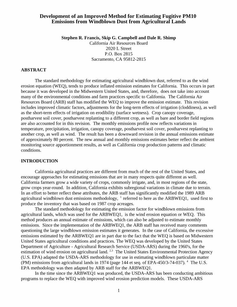
Figure 1 shows the ratio of the ARBWEQ2 to the ARBWEQ1 nonpasture emissions for sixrepresentative California counties. This figure only shows nonpasture emissions, since the ARBWEQ2was the first inventory revision which included pasture emissions. Overall, there was a dramatic drop inthe annual emissions estimate of approximately 80% statewide. The amounts of reductions in theemissions estimates did vary significantly between counties. The acreage changes between theARBWEQ1 and the ARBWEQ2, although in some cases significant, were not responsible for thedramatic decreases in the emissions estimates experienced by most counties. The large reductions inannual emissions estimates were due predominantly to the effects of both the annual and the month-basedadjustments introduced in the ARBWEQ2.

Temporal Profile Comparisons

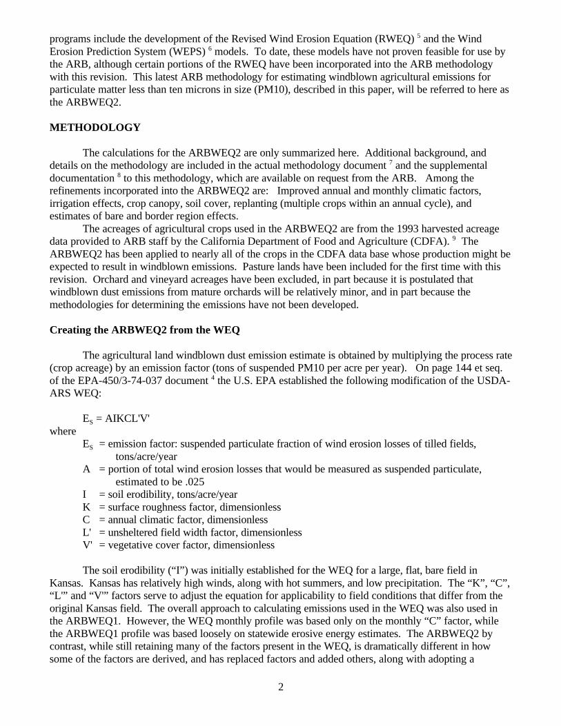
Although annual-based adjustments, such as adjustments to the overall soil erodibility, the long-term erodibility adjustment due to irrigation (cloddiness), and changes to the annual “C” factor causedlarge changes for some counties; much of the decrease in the annual emission estimate between theARBWEQ1 and the ARBWEQ2, reflected in Figure 1, was actually due to the temporal, or monthlyprofile-based adjustments. Several possible temporal profiles are shown in figures 2 and 3 for Fresno

7

County nonpasture and pasture windblown emissions, respectively. It is valid to compare both thenonpasture-based and pasture-based ARBWEQ2 profiles with the same profiles in figures 2 and 3,because, unlike the ARBWEQ2, the other profiles are not crop specific. For the ARBWEQ1, thetemporal profile was based on an estimated statewide erosive wind energy (EWE) profile. This profilewas very flat, and did not adequately reflect the seasonality present in most California counties. The U.S.EPA and USDA-EWE profiles, discussed above in the methods section, were both shifted into the coolerand wetter months (January through March), and were, therefore, also not satisfactory. The profile,implemented in the ARBWEQ2 now includes wind, precipitation and temperature climatic effects, alongwith the addition of the effects of crop canopy, postharvest soil cover, postharvest replanting to adifferent crop, and irrigation. In addition, the inclusion of bare ground and field border effects alsoadjusted the profile in the ARBWEQ2. The ARBWEQ2 profile better reflects the California seasonality,as well as the nonclimatic influences that cause monthly emissions to vary. The ARBWEQ2 nonpasture temporal profiles for Fresno and San Joaquin counties are comparedin Figure 4. The Fresno profile is low in the wet months of November through March, and then jumpsdramatically in April due to the combination of the planting of Cotton (which is by far the largest crop inFresno County), lower precipitation, and increased wind. The net result is that large acreages of freshlyplanted land, with little ground cover, and lower soil moisture are exposed to higher wind speeds. However, the Fresno profile then drops off sharply due mostly to the maturation of the cotton crop (aswell as other crops planted in the same time period) increasing the ground cover. There is a small peakagain in late summer to early fall, due mostly to crop harvesting decreasing the ground cover, after whichthe emissions drop off primarily due to a combination of increasing precipitation, decreasing temperatureand lower wind speeds. The San Joaquin County profile is similar for much of the year, with theexception of the lack of the large Spring peak. The Spring peak is missing because San Joaquin Countyis not dominated by a single crop, like cotton, with a relatively narrow planting window.

The ARBWEQ2 pasture temporal profiles for Fresno and San Joaquin counties, shown inFigure 5, follow basically the same pattern as the cotton dominated Fresno County nonpasture profile,because they reflect a single crop. However, there is a strong Fall peak as well, because the fieldpreparation and planting for pasture are split between the late Spring and early Fall months.

Examining Contributions to the Estimate Reduction, and Validating the Estimate

With so many new features in the ARBWEQ2, it is important to understand how each change hasaffected the emissions estimates. The annual “C” factor and STATSGO-based erodibility changes weresignificant in some cases, and were responsible for some, but not the major portion of the emissionsdecreases between the ARBWEQ1 and the ARBWEQ2. The short-term irrigation factor (wetness) mayreduce the emissions by 10% to 20% during the months when the “C” factor profile peaks. Emissions arealso reduced due to the postharvest soil cover, and the replant factor, but these are occurring duringperiods when the “C” factor profile is lower, and so have less of an effect. For most counties, the largestportions of the emission reductions between the ARBWEQ1 and the ARBWEQ2 estimates are due to thelong term irrigation factor (cloddiness) adjustments (which in some cases decrease the emissions estimateby one-third), and the combination of the “C” factor profile and the crop canopy cover. The reductionsdue to the combination of the “C” factor profile and the crop canopy cover are large for many importantcrops, because the large monthly climatic factors in the summer shift the emissions into the summermonths, when many crop canopy covers are at their maximum.

Existing air pollution monitoring source apportionment data support the decrease in the annualwindblown agricultural PM10 estimate from the ARBWEQ1 to the ARBWEQ2, as well as supporting theARBWEQ2 temporal profile over the ARBWEQ1 profile and other alternative profiles discussedhere. 19,20,21,22

8

GIS Map

The GIS-produced map in Figure 6, shows how the estimated emissions are distributedthroughout the SJV. The map reflects the amount of emissions coming from each of the 4 km grid cells.2

This is not the same as the emissions per cultivated acre, which is the value actually used as the emissionfactor. Nevertheless, the map does reflect well the expected distribution of windblown agriculturalemissions throughout the SJV. The higher emission areas in Kings County and the western portion ofFresno County reflect the region in the SJV with the highest climatic factors, large cultivated touncultivated land ratios, and an overall intermediate crop emissivity. The higher emissivity crops tend tobe those that have lower soil cover during the times when the climatic factor is high. Shorter growingseason crops, such as lettuce and cantaloupe, will have more frequent periods of low canopy cover,which will often coincide with periods of the year having higher climatic factors. If not for Cotton’s longgrowing season, when canopy cover is maintained for a long period, the emission levels in the westernFresno County and Kings County would be much higher. The relatively low emissions in San JoaquinCounty are due in large part both to the crop mix, and the lower annual climatic factor.

CONCLUSIONS

The ARBWEQ2 is much more California-specific than the ARBWEQ1, which was for the most part adirect implementation of the U.S. EPA’s WEQ. Currently available emission source apportionment dataindicate that the ARBWEQ2 is a major improvement with respect to both the annual emissions estimateand the monthly emissions profile.

ACKNOWLEDGMENTS

Although not directly referenced in this paper, numerous agricultural experts from production agriculture,government and academia helped to provide the data inputs for specific crops, conditions, agriculturalpractices, etc. These individuals and organizations are specifically listed in references 7 and 8. Thismethodology also builds on the work of Agnes Dugyon and Krista Eley of the ARB staff, who wereresponsible for previous ARB implementations of the WEQ methodology.

DISCLAIMER

This report has been reviewed by the staff of the California Air Resources Board and approved forrelease. Approval does not signify that the contents necessarily reflect the views and policies of the AirResources Board. Mention of trade names or commercial products does not constitute endorsement orrecommendation for use.

REFERENCES

1. Dugyon, A. Windblown Dust - Agricultural Lands, Section 7.11 of the Stationary Source InventoryMethodology; California Air Resources Board, Sacramento, CA, 1989.

2. Woodruff, N.P.; Siddoway, F.H. “A Wind Erosion Equation”, Soil Sci. Am. Proc. 1965, 29(5), 602-608.

3. Skidmore, E.L.; Woodruff, N.P. Wind Erosion Forces in the United States and Their Use inPredicting Soil Loss; U.S. Department of Agriculture, Agricultural Research Service, 1968;Agriculture Handbook No. 346.

4. Development of Emission Factors for Fugitive Dust Sources; U.S. Environmental Protection Agency,Research Triangle Park, NC, 1974; EPA-450/3-74-037, pp 144-163.

9

5. Revised Wind Erosion Equation; U.S. Department of Agriculture, Agricultural Research Service, BigSpring, TX, 1996.

6. Wind Erosion Prediction System; U. S. Department of Agriculture, Agricultural Research Service,Manhattan, KS, 1995.

7. Francis, S.R. Windblown Dust - Agricultural Lands, Section 7.11 of the Stationary Source InventoryMethodology; California Air Resources Board, Sacramento, CA, 1997.

8. Francis, S.R. Supplemental Documentation for Windblown Dust - Agricultural Lands, Section 7.11of the Stationary Source Inventory Methodology; California Air Resources Board, Sacramento, CA,1997.

9. Eley, K.A. 1995. California Air Resources Board, Sacramento, CA, personal communication. 10. Generalized Soil Map of California; University of California, Division of Agricultural Sciences,

Agricultural Sciences Publications, Richmond, CA, 1980.11. State Geographic Data Base; U. S. Department of Agriculture, Natural Resources Conservation

Service, 1995.12. Hagen, L.J. 1995. U.S. Department of Agriculture, Agricultural Research Service, Manhattan, KS,

personal communication.13. Chow, J.C.; Watson, J.G.; Houck, J.E.; Pritchett, L.C.; Rogers, C.F.; Frazier, C.A.; Egami, R.T.;

Ball, B.M. “A Laboratory Resuspension Chamber to Measure Fugitive Dust Size Distributions andChemical Compositions”, Atmos. Environ. 1994, 28(21), 3463-3481.

14. Bunter, W. 1996. U.S. Department of Agriculture, Natural Resources Conservation Service, Davis,CA, personal communication.

15. Annual Wind Erosion Climatic Factor; United States Department of Agriculture, Natural ResourcesConservation Service, Davis, CA, 1993.

16. California Irrigation Management Information System; Department of Water Resources,Sacramento, CA, 1996.

17. Skidmore, E.L. 1996. U.S. Department of Agriculture, Agricultural Research Service, Manhattan, KS, personal communication.

18. Campbell, S.G.; Shimp, D.R.; Francis, S.R. “Spatial Distribution of PM10 Emissions fromAgricultural Tilling in the San Joaquin Valley”. In Geographic Information Systems inEnvironmental Resources Management; Air & Waste Management Association: Reno, NV, 1996; pp 119-127.

19. Chow, J.C.; Watson, J.G.; Lowenthal, D.H.; Solomon, P.A.; Magliano, K.L.; Ziman, S.D.;Richards, L.W. “PM10 Source Apportionment in California’s San Joaquin Valley”, Atmos. Environ.1992, 26A(18), 3335-3354.

20. Watson, J.G.; Chow, J.C. “PM10 and PM2.5 Variations in Time and Space”; DRIDocument 4204.1F, Desert Research Institute, Reno, NV. 1995.

21. Chow, J.C.; Watson, J.G.; Lowenthal, D.H. “PM10 and PM2.5 Compositions in California’s SanJoaquin Valley”, Aeros. Sci. Tech. 1993, 18, 105-128.

22. Chow, J.C.; Watson, J.G.; Lu, Z.; Lowenthal, D.H.; Frazier, C.A.; Solomon, P.A.; Thuillier, R.H.;Magliano, K.L. “Descriptive Analysis of PM2.5 and PM10 at Regionally Representative LocationsDuring SJVAQS/AUSPEX”, Atmos. Environ. 1996, 30(12), 2079-2112.

Monterey Colusa SanJoaquin Fresno Kern Imperial

0

0.1

0.2

0.3

0.4

0.5

10

Figure 1: Ratio of nonpasture emissions: ARBWEQ2/ARBWEQ1.

Figure 2: Fresno County nonpasture agricultural windblown emission profiles.

11

Figure 3. Fresno County pasture windblown emission profiles.

Figure 4. Nonpasture emission profiles. Figure 5. Pasture emission profiles.

KERN

FRESNO

TULARE

MADERAMERCED

KINGS

SAN JOAQUIN

STANISLAUS

Tons PM10 Emitted per 4km^20 - 22 - 1515 - 3030 - 40

California Environmental Protection AgencyAir Resources Board

N

(No Land Use Data)

C A L I F O R N I A

N E V A D A

P A C I F I C O C E A N

0 10 20 30 40 MilesTSDSC9_97

12

Figure 6: Annual PM10 emissions distribution in the SJV using the ARBWEQ2.

13

Keywords: Agricultural windblown dust, California Air Resources Board, emissions inventory,PM10, wind erosion equation, WEQ.