runoff curve number and saturated hydraulic conductivity ... · "runoff curve number and...

Elhakeem, M. and A.N. Papanicolaou. 2012. "Runoff Curve Number and Saturated Hydraulic Conductivity Estimation via Direct Rainfall Simulator Measurements." Journal of Water Management Modeling R245-09. doi: 10.14796/JWMM.R245-09.© CHI 2012 www.chijournal.org ISSN: 2292-6062 (Formerly in On Modeling Urban Water Systems. ISBN: 978-0-9808853-7-8).

141

9 Runoff Curve Number and Saturated Hydraulic Conductivity Estimation via

Direct Rainfall Simulator Measurements Mohamed Elhakeem and Athanasios N. Papanicolaou

Surface runoff can be estimated directly from conceptual models such as the runoff curve number (RCN) method or indirectly from physically based infiltra-tion models such as the Green–Ampt method (Ponce, 1989; McCuen, 2003; Mishra and Singh, 2003). Both methods are widely accepted models for pre-dicting surface runoff in both agricultural and urbanized watersheds due to their simplicity and to the limited number of parameters required for runoff predic-tion. In addition, they have been integrated into many hydrologic, storm water management and water quality models such as the erosion productivity impact calculator EPIC (Sharpley and Williams, 1990), the soil and water assessment tool SWAT (Arnold et al., 1998), and the stormwater management model SWMM (Rossman et al., 2003). The key parameters involved in the RCN and the Green–Ampt methods are the runoff curve number (CN) and the saturated hydraulic conductivity (Ksat) respectively, which can be obtained from tables as functions of soil texture, management practice, and land use. The use of singular tabulated CN and Ksat values without verification can result in large errors in predicting surface runoff.

Frequent flooding in the Midwest over the past two decades (e.g. 1993, 2008) has raised the need for revised CN and Ksat values to accurately estimate the surface runoff of different watersheds. In this present study, the authors estimated ranges of CN and Ksat values for the different hydrologic soil groups in Iowa, which was affected by devastating flooding in 2008 and 2011. Repre-sentative counties from Iowa with different soils were chosen to estimate the CN and Ksat values. This chapter describes detailed methodological steps to

http://dx.doi.org/10.14796/JWMM.R245-09

142 Runoff Curve Number and Saturated Hydraulic Conductivity …

estimate in situ runoff CN and Ksat values from rainfall simulators. This is useful because the rainfall simulators eliminate the need for natural storm events, and their intensity can be adjusted during an experimental run to mimic natural rain.

9.1 Methodology

9.1.1 Test Bed Matrix

An important element in the field experiments of this study was the selection of a test bed matrix based on soil texture. Based on a preliminary assessment and the recommendations of local Natural Resources Conservation Service offices, test beds were selected in the following counties: Buchanan, Fayette, Pocahon-tas, Cass, Adams and Union (Figure 9.1). These counties have different soil textures varying from sandy to heavy clays representing the four hydrologic soil groups (HSGs). Specifically, Buchanan County with Sparta soil is HSG A, Fayette County with Fayette soil, Pocahontas County with Clarion soil, and Cass County with Marshall soil are HSG B, Adams County with Adair soil is HSG C, and Union County with Clarinda soil is HSG D. Iowa soils are predom-inately HSG B; therefore, three counties with HSG B were selected (Table 9.1).

Figure 9.1 Selected counties representing different soil types in Iowa.

2

5 6

4

1 3

County Soil series HSG 1. Buchanan Sparta A 2. Fayette Fayette B 3. Pocahontas Clarion B 4. Cass Marshall B 5. Adams Adair C 6. Union Clarinda D

1

Runoff Curve Number and Saturated Hydraulic Conductivity … 143

Soil cores 0.1 m diameter and 2.0 m deep were collected from representative fields via a truck-mounted Giddings probe to confirm the soil series and related HSG of each field corresponded to the reported series in the soil survey manual (USDA, 1986). The physical properties of the soil (texture, color and structure) were described in the field to identify the soil series using standard methods (USDA, 1993). For most of the cores, surface soil textures were in the appro-priate ranges for the predetermined HSG in each county (Table 9.1).

Table 9.1 Summary of the core sampling results according to the USDA (1993) classification.

County Buchanan Fayette Pocahontas Cass Adams Union Soil series Sparta Fayette Clarion Marshall Adair Clarinda Reported HSG A B B B C D

Core ST HSG ST HSG ST HSG ST HSG ST HSG ST HSG 1 S A SiL B CL B/C SiCL B/D CL C SiCL D 2 S A SiL B CL B/C SiCL B/D CL C SiCL D 3 SL A SiL B L B SiCL B/D SiCL C/D SiCL D 4 SL A SiL B SCL B SiL B SiCL C/D SiCL D 5 S A SiL B L B CL C SiCL D 6 S A SiCL B/D SCL B CL C SiCL D

ST = surface texture; HSG = hydrologic soil group; S = sand; SL = sandy-loam; SCL = sandy-clay-loam; SiL = silty-loam; Si = silt; CL = clay-loam; SiCL = silty-clay-loam; SiC = silty-clay.

9.1.2 Field Measurements

Equipment

The experiments were conducted using three Norton ladder multiple intensity rainfall simulators (Figure 9.2) manufactured by the USDA-ARS National Soil Erosion Research Laboratory in West Lafayette, Indiana (Norton, 2006). The rainfall simulators eliminate the need for natural storm events and rainfall intensity, and can be adjusted during an experimental run to mimic natural rain (Auerswald and Haider, 1996). They are calibrated against natural rainfall considering drop size distribution, spatial uniformity and fall velocity (Frasson et al., 2011).

The basic unit of each simulator consists of an aluminum frame 2.5 m long, 1.5 m wide and 2.7 m high. The frame has four telescopic legs to maintain stability and the vertical orientation of the nozzles. The frame was a self con-tained unit that includes two nozzles spaced 1.1 m apart, piping, an oscillating mechanism and a drive motor. The nozzles (Figure 9.2) provided spherical drops with a median diameter of 2.25 mm and a maximum rainfall intensity of 235 mm/h. The simulator’s rainfall intensity can be changed instantaneously, from a controller, during a simulation event. The simulators were equipped with


storage tanks and a water pump with a system of valves that allowed rainfall intensity to be independently adjusted for each simulator. Galvanized metal sheets (Figure 9.2) were used for plot borders. Wind shields (Figure 9.2) of slightly porous fabric sheets were used to avoid wind influence.

Figure 9.2 General view of the rainfall simulators (on the top right is the simulator nozzle).

Calibration

Previous studies with rainfall simulators have shown that rainfall events of 3 h duration are sufficient to guarantee steady state condition for field measure-ments of surface runoff (Auerswald and Haider, 1996; Jain et al., 2006). The maximum 3 h rainfall depths of different return periods for Iowa (Table 9.2) were obtained from the United States rainfall distribution maps and the SCS 24 h Type II rainfall distribution (Figure 9.3a).

Table 9.2 Rainfall depths for different return periods in Iowa.

Return period (y) 2 5 10 25 50 100 24 h rainfall depth (mm) 84 102 114 140 152 160 3 h rainfall depth (mm) 50 61 68 83 90 95

Water tanks

Wind shields

Test plots & borders

Simulators water line Simulators frame & legs Water jet


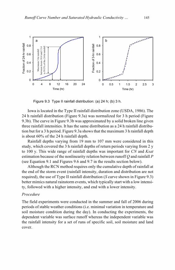
Figure 9.3 Type II rainfall distribution: (a) 24 h; (b) 3 h.

Iowa is located in the Type II rainfall distribution zone (USDA, 1986). The 24 h rainfall distribution (Figure 9.3a) was normalized for 3 h period (Figure 9.3b). The curve in Figure 9.3b was approximated by a solid broken line given three rainfall intensities. It has the same distribution as a 24 h rainfall distribu-tion but for a 3 h period. Figure 9.3a shows that the maximum 3 h rainfall depth is about 60% of the 24 h rainfall depth.

Rainfall depths varying from 19 mm to 107 mm were considered in this study, which covered the 3 h rainfall depths of return periods varying from 2 y to 100 y. This wide range of rainfall depths was important for CN and Ksat estimation because of the nonlinearity relation between runoff Q and rainfall P (see Equation 9.1 and Figures 9.6 and 9.7 in the results section below).

Although the RCN method requires only the cumulative depth of rainfall at the end of the storm event (rainfall intensity, duration and distribution are not required), the use of Type II rainfall distribution (S curve shown in Figure 9.3) better mimics natural rainstorm events, which typically start with a low intensi-ty, followed with a higher intensity, and end with a lower intensity.

Procedure

The field experiments were conducted in the summer and fall of 2006 during periods of stable weather conditions (i.e. minimal variation in temperature and soil moisture condition during the day). In conducting the experiments, the dependent variable was surface runoff whereas the independent variable was the rainfall intensity for a set of runs of specific soil, soil moisture and land cover.

0

0.2

0.4

0.6

0.8

1

0 4 8 12 16 20 24Time (hr)

Frac

tion

of 2

4-hr

rain

fall

aM

axim

um 3

-hr r

ainf

all

betw

een

hour

s 10.

4 an

d 13

.4

is 5

9.5%

of t

he 2

4-hr

rain

fall

0

0.2

0.4

0.6

0.8

1

0 0.5 1 1.5 2 2.5 3Time (hr)

Frac

tion

of 3

-hr r

ainf

all

b


The slope effect on surface runoff was controlled by selecting fields of very mild slopes (<0.05%), which are representative of the average condition found in Iowa. This was confirmed via surveying. The effect of soil moisture was minimized by using three plots per field instead of a single plot (Figure 9.2 above). Six runs were conducted in each experimental plot.

The experimental procedure to conduct the experimental runs was as fol-lows. The three rainfall simulators were installed at the selected fields with minimum disturbance. The experimental plots (each 1.5 m × 2.5 m) were installed adjacent to one another to limit spatial variability in soil properties (Figure 9.2 above) and to allow for simultaneous measurements of three differ-ent rainfall intensities. Initial soil moisture in each plot was measured via a tensiometer (Figures 9.4a and 9.4b) at 15 cm and 30 cm depths from the soil surface before each run. The variation was less than 10% between the two depths.

Figure 9.4 Field measurements of surface runoff: (a and b) measuring initial moisture condition via a tensiometer; and (c) collecting runoff from the plot.

After measuring soil moisture, each simulator was set to a certain rainfall intensity following the rainfall distribution curve shown in Fig. 9.3b, starting with a low intensity, followed with a higher intensity, and ending with a lower intensity. During the experimental run, runoff was collected from a small pipe connected to the plot borders via small graduated bottles of known volume (Figure 9.4c).

After each run, the rainfall simulator was stopped to allow the plots to drain before starting the next run. The time required for the plot to drain varied from 15 min to 45 min, depending on the tested soils texture and residue. Figure 9.5 shows a conceptual sketch explaining the proposed methodology for measuring surface runoff. The figure shows the distribution of the rainfall intensity (p) and corresponding runoff rate (q) in mm/h. The accumulated volumes of rainfall (P) and runoff (Q) in mm are also shown in Figure 9.5.

c ba


Figure 9.5 A conceptual sketch explaining the methodology during tests: The sketch shows the rainfall–runoff trends in one plot for 1.5 subsequent runs and the draining time for the plot.

9.2 Results and Discussions

The curve number (CN) is an index representing the soil cover complex that reflects the response of a specific soil, under certain conditions (soil moisture and land cover), to a rainstorm event through runoff and infiltration (Bales and Betson, 1981). CN is a non-dimensional index having theoretically a value between 0 (no runoff) and 100 (no infiltration). For a specific soil cover condi-tion, CN can be obtained from a range of rainfall depths and corresponding runoff depths (Figure 9.6) by solving for S and Ia using the following CN equations:

(9.1)

Cum

ulati

ve (m

m)

Inten

sity

(mm

/hr)

Draining time

a

a

ISPIPQ−+

−=2)(


(9.2)

where: Q = direct runoff depth (mm), P = rainfall depth (mm), S = potential maximum retention (mm), and

Ia = initial abstraction (i.e. amounts of interception, infiltra-tion, surface storage, etc.) before runoff takes place (mm).

Figure 9.6 Method of CN estimate from data obtained via the rainfall simulators at the second field in Fayette County, Iowa during summer 2006.

The relationship between rainfall and runoff described by Equation 9.1 re-quires the use of nonlinear regression analysis methods (Shahin et al., 1993; Draper and Smith, 1998) to obtain S and Ia values. Values of S and Ia were applied iteratively to Equation 9.1 to produce a curve that best represents the measured data in Figure 9.6. The solid line in Figure 9.6 represents Equation 9.1 using the optimal S and Ia values, whereas the dots represent the measured values for site 2 found in Fayette County. The intercept of the solid line with the x-axis gives Ia. The CN value was obtained from Equation 9.2.

When infiltration rate reaches a steady state condition (i.e. rates do not change with respect to time), this is defined in the literature as the saturated hydraulic conductivity, or Ksat (Gupta et al., 1996; Papanicolaou et al., 2009).

25425400 −=CN

S

0

20

40

60

80

0 20 40 60 80 100 120Rainfall P (mm)

Run

off Q

(mm

)

MeasuredFitted


Ksat can be estimated from a range of data obtained via the rainfall simulators using the following mass balance equation:

(9.3)

where: f = infiltration rate (mm/h), p = rainfall intensity (mm/h), and q = runoff rate (mm/h).

In Equation 9.3 the storage and evaporation are considered negligible and ignored due to the short duration of the rainfall experiments and relatively small size of the rainfall simulation plots. Ksat can be obtained from Equation 9.3 by plotting f versus p (Figure 9.7). Figure 9.7 provides an example of the measured rainfall and infiltration values shown in dots, whereas the solid line represents the Ksat value for site 2 found in Fayette County. The figure indicates that the infiltration rate has reached a steady state condition through the rainfall simula-tor measurements, which corresponds to Ksat.

Figure 9.7 Method of Ksat estimate from data obtained via the rainfall simulators at the second field in Fayette County, Iowa during summer 2006.

A summary of the CN and Ksat data for the different sites is given in Table 9.3. The county name and sites per county are shown in the first two columns. Columns 3–7 and 8–12 summarize the data for the summer and fall seasons, respectively. S values in columns 3 and 8, and Ia values in columns 4 and 9 provide the best fit of Equation 9.1 to the measured data. The CN values in

qpf −=

0

20

40

60

80

100

120

0 50 100 150 200 250Rainfall p (mm/hr)

Infil

tratio

n f =

p -

q (m

m/h

r) Ksat


columns 5 and 10 were estimated using Equation 9.2. Columns 6 and 11 pro-vide Ksat. Columns 7 and 12 provide the measured percentage of the volumet-ric soil water content (M) obtained via the tensiometer. M theoretically varies between 0 for dry soil and 100 for a saturated soil.

Table 9.3 Summary of the CN and Ksat results.

The CN values were generally lower in the fall compared to the summer (Table 9.3). The difference between fall and summer values (deviation of about 30%) was attributed to the land cover (amounts of residue found on the test plots at those times), which controls the surface runoff (Rawls et al., 1980). In the fall a higher residue cover level of 0.8 reduced surface runoff and the CN values due to added roughness effects (Papanicolaou and Abaci, 2008). In summer the residue level dropped to 0.18, allowing more surface runoff. Simi-lar observations have been reported for Ksat which had higher values in fall than in summer. This finding suggests again lower surface runoff in the fall compared to the summer. Papanicolaou and Abaci 2008 have shown that failure to adjust CN and Ksat values through the year can result in an overestimation of annual surface runoff. Thus CN and Ksat should be treated as dynamic varia-bles varying throughout the year (Hjelmfelt et al., 1982; McCuen, 2002; Schneider and McCuen, 2005).

Higher soil moisture (M) conditions were also observed in fall than in summer (Table 9.3). This was attributed to lower temperature and higher residue cover, which minimized evaporation from the soil surface (Linsley et al., 1982). In summer, lower residue cover and higher temperature increased

(1) County

(2) Site

Measured summer data Measured fall data (3) S

(mm)

(4) Ia

(mm)

(5) CN

(6) Ksat

(mm/h)

(7) M %

(8) S

(mm)

(9) Ia

(mm)

(10) CN

(11) Ksat

(mm/h)

(12) M %

Buchan-an

1 148 21 63 150 30 148 13 63 147 70 2 170 23 60 163 40 767 53 25 203 46 3 257 65 50 168 26 1285 101 17 218 36

Fayette 1 25 1 91 51 93 178 13 59 127 60 2 64 13 80 89 44 152 7 63 119 64 3 85 20 75 132 41 135 8 65 130 70

Poca-hontas

1 142 33 64 140 31 204 17 56 122 60 2 17 2 94 51 70 52 3 83 69 90 3 61 5 81 86 52 86 5 75 91 82

Cass 1 63 7 80 84 52 107 7 70 94 70 2 34 3 88 66 55 51 3 83 64 90 3 71 13 78 114 46 71 5 78 91 90

Adams 1 67 15 79 109 36 84 5 75 102 82 2 45 6 85 84 48 114 9 69 117 70 3 29 3 90 64 61 71 6 78 84 82

Union 1 13 1 95 56 90 82 6 76 81 79 2 48 8 84 81 41 87 5 75 99 77 3 6 1 98 23 97 38 2 87 66 95


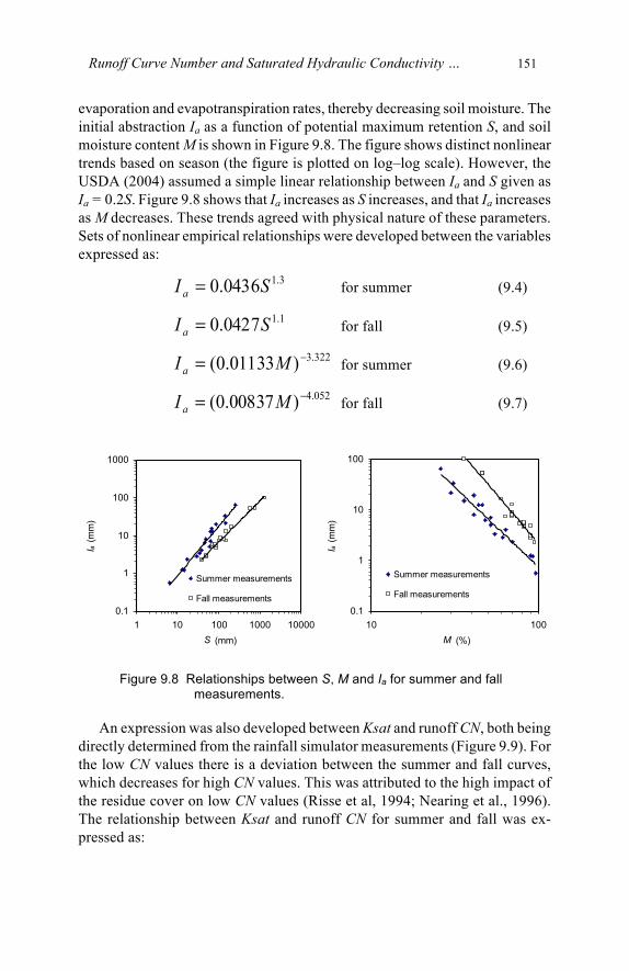
evaporation and evapotranspiration rates, thereby decreasing soil moisture. The initial abstraction Ia as a function of potential maximum retention S, and soil moisture content M is shown in Figure 9.8. The figure shows distinct nonlinear trends based on season (the figure is plotted on log–log scale). However, the USDA (2004) assumed a simple linear relationship between Ia and S given as Ia = 0.2S. Figure 9.8 shows that Ia increases as S increases, and that Ia increases as M decreases. These trends agreed with physical nature of these parameters. Sets of nonlinear empirical relationships were developed between the variables expressed as:

for summer (9.4)

for fall (9.5)

for summer (9.6)

for fall (9.7)

Figure 9.8 Relationships between S, M and Ia for summer and fall measurements.

An expression was also developed between Ksat and runoff CN, both being directly determined from the rainfall simulator measurements (Figure 9.9). For the low CN values there is a deviation between the summer and fall curves, which decreases for high CN values. This was attributed to the high impact of the residue cover on low CN values (Risse et al, 1994; Nearing et al., 1996). The relationship between Ksat and runoff CN for summer and fall was ex-pressed as:

3.10436.0 SIa =1.10427.0 SIa =

322.3)01133.0( −= MIa052.4)00837.0( −= MIa

0.1

1

10

100

1000

1 10 100 1000 10000S (mm)

I a (m

m)

Summer measurements

Fall measurements0.1

1

10

100

10 100M (%)

I a (m

m)

Summer measurements

Fall measurements


for summer (9.8)

for fall (9.9)

Figure 9.9 Ksat versus runoff CN obtained from the rainfall simulator measurements.

Scale is an important factor to consider when characterizing heterogeneity of landscape attributes and surface runoff (Beven, 1983; Bhuyan et al., 2003). A single CN or Ksat value may not represent the watershed characteristics because of the expected variability in soil texture, average slope, moisture condition, land use and cover. However, within the field scale, the variability in these factors may be small, and thus a single CN or Ksat value may represent the field (West et al., 2008). Under this condition, the CN and Ksat values obtained from an experimental plot may represent the CN and Ksat values of a tested field. However, this requires that the experimental plot have similar characteristics as the field in terms of soil texture, average slope, moisture condition, land use and cover.

At the development stages of an experimental test bed matrix, the locations of the plots within the fields can be obtained from digital elevation and soil maps such as the United States Department of Agriculture’s Soil Survey Geo-graphic database. However, the selected locations must be verified later via surveying and core sampling. The data obtained from different fields within a watershed can be integrated to obtain representative CN and Ksat values reflect-

109304.0 +−= KsatCN114423.0 +−= KsatCN

20

40

60

80

100

0 50 100 150 200 250Ksat (mm/hr)

CN

summerfall


ing the watershed characteristics. These data can be used to calibrate different hydrologic, storm water management and water quality models.

9.3 Conclusions

This study provided detailed methodological steps to estimate in situ runoff curve number (CN) and saturated hydraulic conductivity (Ksat) using rainfall simulators. Representative fields from six counties of Iowa with different soils were chosen to estimate the CN and Ksat. The study estimated a range of CN and Ksat values for the summer and fall seasons, which can allow for more accurate estimates of surface runoff.

The following points summarize the findings of this research: 1. Rainfall simulators are reliable instruments for estimating in situ

runoff CN and Ksat because they eliminate the need for natural storm events and rainfall intensity can be adjusted during an ex-perimental run to mimic natural rain;

2. A range of CN values was established for the summer and fallseasons. The range of the estimated CN values in fall was gener-ally lower than the summer CN values with a deviation of about 30%. This was attributed to the seasonal change in the fields land cover and soil moisture conditions;

3. Initial abstraction Ia was not linearly proportional to potentialmaximum retention S (i.e. Ia ≠ 0.2S) and increases with decrease of soil moisture M; and

4. CN is interrelated with Ksat, showing an inversely proportionalrelationship between the two variables. However, a unique rela-tionship does not exist as two curves were observed, based on seasonality.

References Arnold J.G., Srinivasan R., Muttiah R.S. and Williams J.R. (1998). Large area hydrologic

modeling and assessment Part 1: Model development. Journal of the American Water Resources Association, 34(1), 73-89.

Auerswald K. and Haider J. (1996). Runoff curve numbers for small grain under German cropping conditions. Journal of Environmental Management, 47, 223-228.

Bales J. and Betson R.P. (1981). The curve number as a hydrologic index. In Singh V.P. (ed) Rainfall Runoff Relationship, Water Resources Publication, Littleton, CO, pp. 371-386.

Beven K. (1983). Surface water hydrology-runoff generation and basin structure. Review Geophysics, 21(3), 721-730.


Bhuyan S.J., Mankin K.R. and Koelliker J.K. (2003). Watershed-scale AMC selection for hydrologic modeling. Transactions of the American Society of Agricultural Engi-neers, 46, 237-244.

Draper N. and Smith H. (1998). Applied Regression Analysis. 3rd edn., John Wiley Sons Inc., New York.

Frasson R.P.M., Krajewski W.F. and Cunha L.K. (2011). Performance assessment of the Theis optical disdrometer. Atmospheric Research, 101, 237-255.

Gupta N., Rudra R.P. and Parkin G. (1996). Analysis of spatial variability of hydraulic conductivity at field scale. Canadian Biosystems Engineering, 48(1), 55-62.

Hjelmfelt A.T., Kramer L.A. and Burwell R.E. (1982). Curve numbers as random variables. Proceedings of the International Symposium on Rainfall-Runoff Modeling, Water Resources Publishers, Littleton, CO, 365-373.

Jain M.K., Mishra S.K., Babu P.S., Venugopal K. and Singh V.P. (2006). Enhanced runoff curve number model incorporating storm duration and a nonlinear Ia-S rela-tion. J Hydrologic Engineering, 11(6), 631-635.

Linsley R.K., Kohler M.A. and Paulhus J.L. (1982). Hydrology for Engineers. 3rd edn., McGraw-Hill Inc., New York.

McCuen R.H. (2002). Approach to confidence interval estimation for curve numbers. Journal of Hydrologic Engineering, 7(1), 43-48.

McCuen R.H. (2003). Hydrologic Analysis and Design. 3rd edn., Prentice Hall, New Jersey.

Mishra S.K. and Singh V.P. (2003). Soil conservation service curve number (SCS-CN) methodology. Kluwer Academic, Dordrecht, The Netherlands.

Nearing M.A., Liu B.Y., Risse L.M. and Zhang X.C. (1996). Curve numbers and Green-Ampt effective hydraulic conductivities. Water Resources Bulletin, 32(1), 125-136.

Norton L.D. (2006). A linear variable intensity rainfall simulator for erosion studies. Proc. of 2nd Bieannial Stormwater Management Research Symp, Wanielista, M. and J. Smoot (eds), May 4-5, 2006. Univ. of Central Florida, Orlando, FL, pp. 93-103.

Papanicolaou A.N. and Abaci O. (2008). Upland erosion modeling in a semi-humid environment via the Water Erosion Prediction Project Model. Journal of Irrigation and Drainage Engineering, 134(6), 796-806.

Papanicolaou A.N., Elhakeem M., Wilson C., Burras C.L. and Oneal B. (2009). Observa-tions of soils at the hillslope scale in the Clear Creek Watershed in Iowa, USA. Soil Survey Horizons, Winter 2008 edition, 83-86.

Ponce V.M. (1989). Engineering Hydrology, Principles and Practices. Prentice Hall, Englewood Cliffs, NJ.

Rawls W.J., Onstad C.A. and Richardson H.H. (1980). Residue and tillage effects on SCS runoff curve numbers. Trans. of the American Society of Agricultural Engineers, 23, 357-361.

Risse L.M., Nearing M.A. and Savabi M.R. (1994). Determining the Green-Ampt effective hydraulic conductivity from rainfall-runoff data for the WEPP model. Trans. of the American Society of Agricultural Engineers, 37(2), 411-418.

Rossman, L.A., R.E. Dickinson, T. Schade, C.C. Chan, E. Burgess, D. Sullivan and F. Lai. 2003. "SWMM 5 - the Next Generation of EPA's Storm Water Management Model." Journal of Water Management Modeling R220-16. doi: 10.14796/JWMM.R220-16.

Schneider L.E. and McCuen R.H. (2005). Statistical guidelines for curve number genera-tion. Journal of Irrigation and Drainage Engineering, 131 (3), 282-290.

http://dx.doi.org/10.14796/JWMM.R220-16


Shahin M., van Orschot H.L. and Delange S.J. (1993). Statistical Analysis in Water Resources Engineering. A. A. Balkema, Rotterdam, The Netherlands.

Sharpley A.N. and Williams J.R. (1990). EPIC-Erosion/productivity impact calculator- 1: model documentation. USDA-Technical Bulletin No. 1768, US Government Printing Office, Washington DC.

USDA. (1986). Urban hydrology for small watersheds. Technical Release No. 55 (TR-55), Soil Conservation Service, Washington DC.

USDA. (1993). Soil survey manual. Handbook 18, Soil Conservation Service, Washing-ton DC.

West L.T., Abreu M.A. and Bishop J.P. (2008). Saturated hydraulic conductivity of soils in the Southern Piedmont of Georgia, USA: Field evaluation and relation to horizon and landscape properties. Catena, 73 (2008), 174–179.

runoff curve number and saturated hydraulic conductivity ... · "runoff curve number and...

Documents