s. duplij, constraintless approach to singular theories, new brackets and multi time dynamics
TRANSCRIPT

Constraintless approach to singular theories,new brackets and multi-time dynamics
STEVEN DUPLIJ
Institute of Mathematics, University of Munster
http://wwwmath.uni-muenster.de/u/duplij
11 May 2015
1
Abstract
2
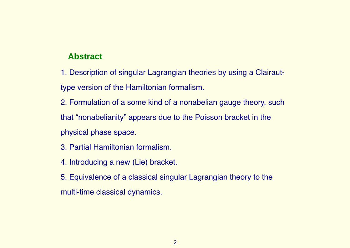
1. Description of singular Lagrangian theories by using a Clairaut-
type version of the Hamiltonian formalism.
2. Formulation of a some kind of a nonabelian gauge theory, such
that “nonabelianity” appears due to the Poisson bracket in the
physical phase space.
3. Partial Hamiltonian formalism.
4. Introducing a new (Lie) bracket.
5. Equivalence of a classical singular Lagrangian theory to the
multi-time classical dynamics.

Introduction
Most fundamental physical models are based on gauge field theories
WEINBERG [2000], DELIGNE ET AL. [1999]. On the classical level they
are described by degenerate Lagrangians, which makes the passage
to Hamiltonian description (necessary for quantization) highly
nontrivial and complicated DIRAC [1964], SUNDERMEYER [1982],
GITMAN AND TYUTIN [1986], REGGE AND TEITELBOIM [1976]. A
common way to deal with such theories is considering the Dirac
approach DIRAC [1964] based on extending the phase space and use
of constraints. In spite of its general success, the Dirac approach has
limited applicability and some inner problems PONS [2005].
3
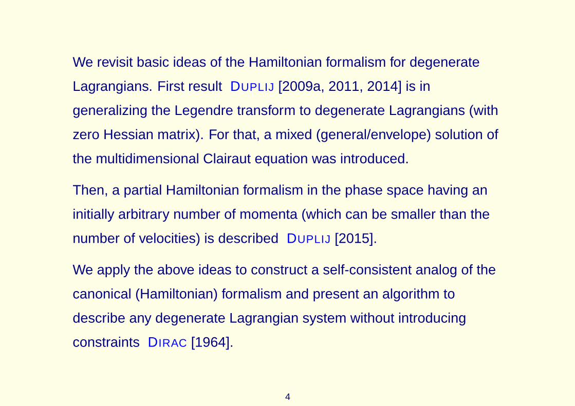
We revisit basic ideas of the Hamiltonian formalism for degenerate
Lagrangians. First result DUPLIJ [2009a, 2011, 2014] is in
generalizing the Legendre transform to degenerate Lagrangians (with
zero Hessian matrix). For that, a mixed (general/envelope) solution of
the multidimensional Clairaut equation was introduced.
Then, a partial Hamiltonian formalism in the phase space having an
initially arbitrary number of momenta (which can be smaller than the
number of velocities) is described DUPLIJ [2015].
We apply the above ideas to construct a self-consistent analog of the
canonical (Hamiltonian) formalism and present an algorithm to
describe any degenerate Lagrangian system without introducing
constraints DIRAC [1964].
4
1 The Legendre-Fenchel and Legendre transforms
1 The Legendre-Fenchel and Legendre transforms
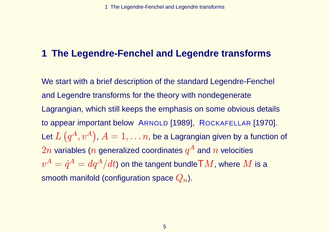
We start with a brief description of the standard Legendre-Fenchel
and Legendre transforms for the theory with nondegenerate
Lagrangian, which still keeps the emphasis on some obvious details
to appear important below ARNOLD [1989], ROCKAFELLAR [1970].
Let L(qA, vA
), A = 1, . . . n, be a Lagrangian given by a function of
2n variables (n generalized coordinates qA and n velocities
vA = qA = dqA/dt) on the tangent bundleTM , whereM is a
smooth manifold (configuration spaceQn).
5

1 The Legendre-Fenchel and Legendre transforms
By the convex approach definition ( ROCKAFELLAR [1967], ARNOLD
[1989]), a HamiltonianH(qA, pA
)is a dual function on the phase
space T∗M (or convex conjugate ROCKAFELLAR [1970]) to the
Lagrangian (in the second set of variables pA) and is constructed by
means of the Legendre-Fenchel transform LLegFen
7−→ HFen defined by
FENCHEL [1949], ROCKAFELLAR [1967]
HFen(qA, pA
)= sup
vAG(qA, vA, pA
), (1.1)
G(qA, vA, pA
)= pAv
A − L(qA, vA
). (1.2)
It was applied to nonconvex ALART ET AL. [2006] and
nondifferentiable VALLEE ET AL. [2004] L, leading to extensions of
the Hamiltonian formalism ( CLARKE [1977], IOFFE [1997]).
6

1 The Legendre-Fenchel and Legendre transforms
In the standard mechanics GOLDSTEIN [1990] one usually restricts to
strictly convex, smooth and differentiable Lagrangians (see, e.g.,
ARNOLD [1989], SUDARSHAN AND MUKUNDA [1974]). Then the
coordinates qA are treated as fixed (passive with respect to the
transform) parameters, and the velocities vA are assumed
independent functions of time. The supremum (1.1) is attained by
finding an extremum point vA = vAextr of the (“pre-Hamiltonian”)
functionG(qA, vA, pA
), which leads to the supremum condition
pB =∂L(qA, vA
)
∂vB
∣∣∣∣∣vA=vAextr
. (1.3)
7

1 The Legendre-Fenchel and Legendre transforms
It is assumed ( ARNOLD [1989], SUDARSHAN AND MUKUNDA [1974],
GOLDSTEIN [1990]) that the only way to get rid of dependence on the
velocities vA in the r.h.s. of (1.1) is to resolve (1.3) and find its
solution given by a set of functions
vAextr = VA(qA, pA
). (1.4)
This can be done only in the class of nondegenerate Lagrangians
L(qA, vA
)= Lnondeg
(qA, vA
)(in the second set of variables vA),
which is equivalent to the Hessian being non-zero
det
∥∥∥∥∥∂2Lnondeg
(qA, vA
)
∂vB∂vC
∥∥∥∥∥6= 0. (1.5)
8

1 The Legendre-Fenchel and Legendre transforms
Then substitute vAextr to (1.1) and obtain the standard Hamiltonian
(see, e.g., ARNOLD [1989], GOLDSTEIN [1990])
H(qA, pA
) def= G
(qA, vAextr, pA
)
= pBVB(qA, pA
)− Lnondeg
(qA, V A
(qA, pA
)). (1.6)
The passage from the nondegenerate Lagrangian Lnondeg(qA, vA
)to
the HamiltonianH(qA, pA
)is called the Legendre transform which
will be denoted by Lnondeg Leg7−→ H .
Geometric viewpoint TULCZYJEW [1989], MARMO ET AL. [1985],
ABRAHAM AND MARSDEN [1978], the Legendre transform being
applied to L(qA, vA
)is tantamount to the Legendre transformation
of the tangent to cotangent bundle Leg : TM → T∗M .
9
2 The Legendre-Clairaut transform
2 The Legendre-Clairaut transform
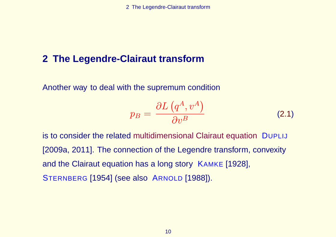
Another way to deal with the supremum condition
pB =∂L(qA, vA
)
∂vB(2.1)
is to consider the related multidimensional Clairaut equation DUPLIJ
[2009a, 2011]. The connection of the Legendre transform, convexity
and the Clairaut equation has a long story KAMKE [1928],
STERNBERG [1954] (see also ARNOLD [1988]).
10

2 The Legendre-Clairaut transform
We differentiate (1.6) by momenta pA and use the supremum
condition (2.1) to obtain
∂H(qA, pA
)
∂pB= V B
(qA, pA
)
+
pC −∂L(qA, vA
)
∂vC
∣∣∣∣∣vC=V C(qA,pA)
∂VC(qA, pA
)
∂pB= V B
(qA, pA
),
(2.2)
which can be called the dual supremum condition (indeed this gives
the first set of the Hamilton equations, see below). The relations (2.1),
(1.6) and (2.2) together represent a particular case of the Donkin
theorem (see e.g. GOLDSTEIN [1990]).
11
2 The Legendre-Clairaut transform
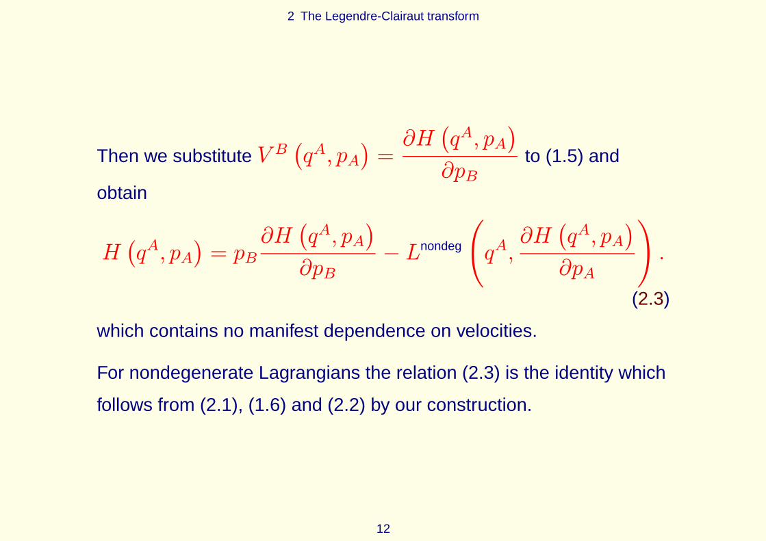
Then we substitute V B(qA, pA
)=∂H
(qA, pA
)
∂pBto (1.5) and
obtain
H(qA, pA
)= pB
∂H(qA, pA
)
∂pB− Lnondeg
(
qA,∂H
(qA, pA
)
∂pA
)
.
(2.3)
which contains no manifest dependence on velocities.
For nondegenerate Lagrangians the relation (2.3) is the identity which
follows from (2.1), (1.6) and (2.2) by our construction.
12

2 The Legendre-Clairaut transform
Main idea: to treat (2.4) by itself (without referring to (2.1), (1.6) and
(2.2)) as a definition of a new transform being a solution of the
following nonlinear partial differential equation (the multidimensional
Clairaut equation) DUPLIJ [2009a, 2011]
HCl(qA, λA
)= λB
∂HCl(qA, λA
)
∂λB−L
(
qA,∂HCl
(qA, λA
)
∂λA
)
,
(2.4)
where λA are parameters and L(qA, vA
)is any differentiable
smooth function of 2n variables (without nondegeneracy condition
(1.5)). Call the transform defined by (2.4) LLegCl
7−→ HCl a Clairaut
duality transform (or Legendre-Clairaut transform) andHCl(qA, λA
)
a Hamilton-Clairaut function DUPLIJ [2009a, 2011, 2014].
13

2 The Legendre-Clairaut transform
Note that pB =∂L(qA, vA
)
∂vBis commonly treated as a definition of
all dynamical momenta pA, but we should distinguish them from the
parameters of the Clairaut duality transform λA.
In our approach before solving Clairaut equation and applying the
supremum condition (2.1) the parameters λA are not related to the
Lagrangian.
The corresponding Legendre-Clairaut transformation is the map
LegCl : TM → T∗ClM, (2.5)
where the space T∗ClM in local coordinates is just(qA, λA
), and we
call T∗ClM a Clairaut phase space. Note T∗ClM is not a cotangent
bundle, but its submanifold can be the cotangent bundle T∗M .
14
3 Construction of the Hamilton-Clairaut function
3 Construction of the Hamilton-Clairaut function
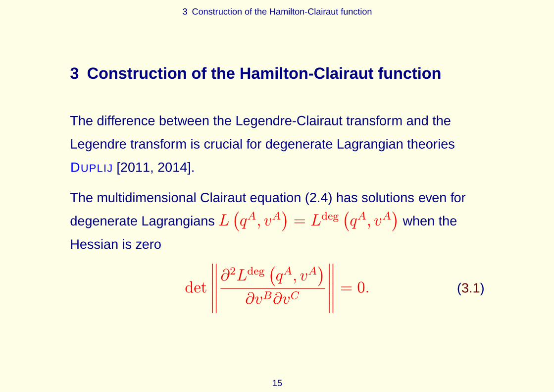
The difference between the Legendre-Clairaut transform and the
Legendre transform is crucial for degenerate Lagrangian theories
DUPLIJ [2011, 2014].
The multidimensional Clairaut equation (2.4) has solutions even for
degenerate Lagrangians L(qA, vA
)= Ldeg
(qA, vA
)when the
Hessian is zero
det
∥∥∥∥∥∂2Ldeg
(qA, vA
)
∂vB∂vC
∥∥∥∥∥= 0. (3.1)
15
3 Construction of the Hamilton-Clairaut function
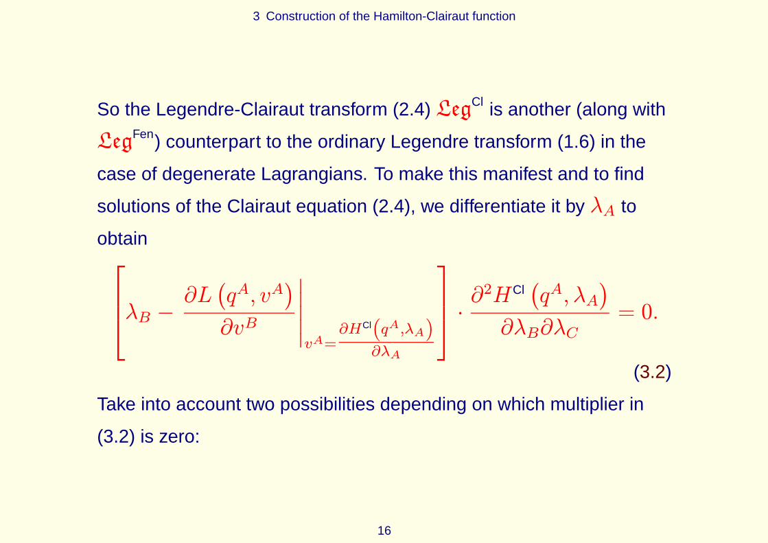
So the Legendre-Clairaut transform (2.4) LegCl is another (along with
LegFen) counterpart to the ordinary Legendre transform (1.6) in the
case of degenerate Lagrangians. To make this manifest and to find
solutions of the Clairaut equation (2.4), we differentiate it by λA to
obtain
λB −
∂L(qA, vA
)
∂vB
∣∣∣∣∣vA=
∂HCl(qA,λA)∂λA
∙∂2HCl
(qA, λA
)
∂λB∂λC= 0.
(3.2)
Take into account two possibilities depending on which multiplier in
(3.2) is zero:
16
3 Construction of the Hamilton-Clairaut function
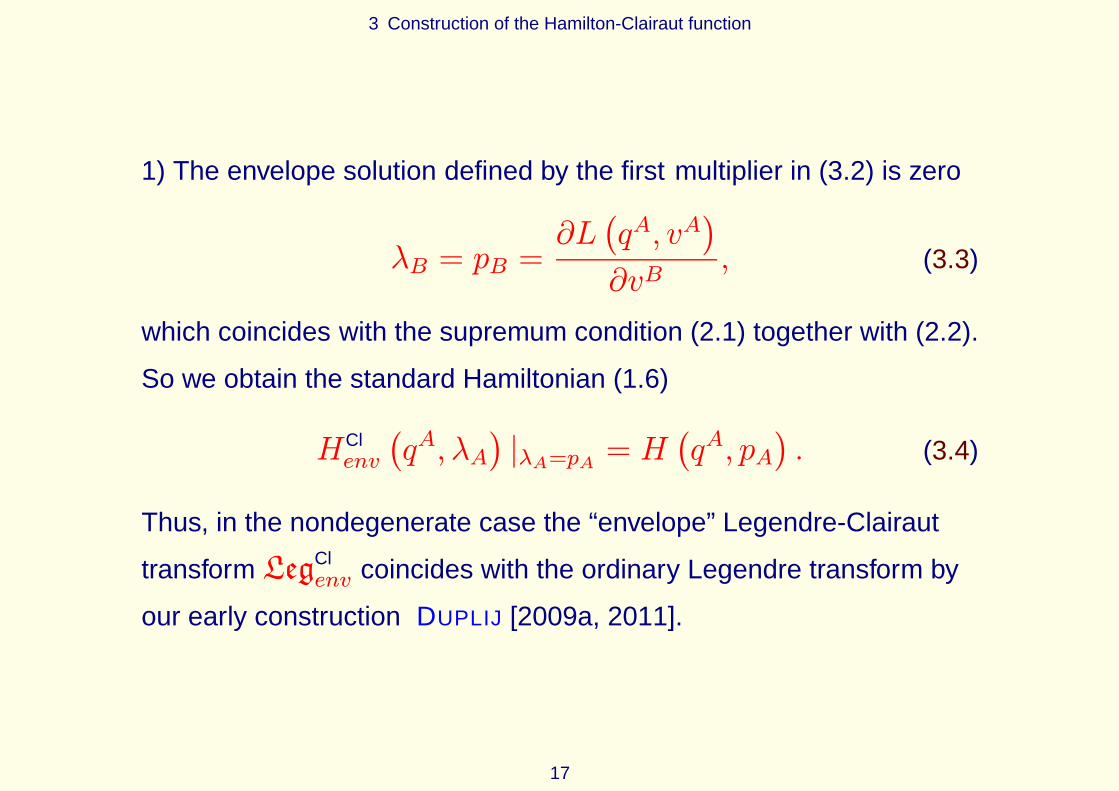
1) The envelope solution defined by the first multiplier in (3.2) is zero
λB = pB =∂L(qA, vA
)
∂vB, (3.3)
which coincides with the supremum condition (2.1) together with (2.2).
So we obtain the standard Hamiltonian (1.6)
HClenv
(qA, λA
)|λA=pA = H
(qA, pA
). (3.4)
Thus, in the nondegenerate case the “envelope” Legendre-Clairaut
transform LegClenv coincides with the ordinary Legendre transform by
our early construction DUPLIJ [2009a, 2011].
17

3 Construction of the Hamilton-Clairaut function
2) A general solution is defined by
∂2HCl(qA, λA
)
∂λA∂λB= 0 (3.5)
which gives∂HCl
(qA, λA
)
∂λB= cB , here cA are smooth functions of
qA, and cA are considered as parameters (passive variables). Then
HClgen
(qA, λA, c
A)= λBc
B − L(qA, cA
), (3.6)
corresponding to a “general” Legendre-Clairaut transform LegClgen.
The general solutionHClgen
(qA, λA, c
A)
is always linear in the
variables λA, which do not coincide with the dynamical momenta pA
i.e. λA 6= pA because we do not have the envelope solution
18
3 Construction of the Hamilton-Clairaut function
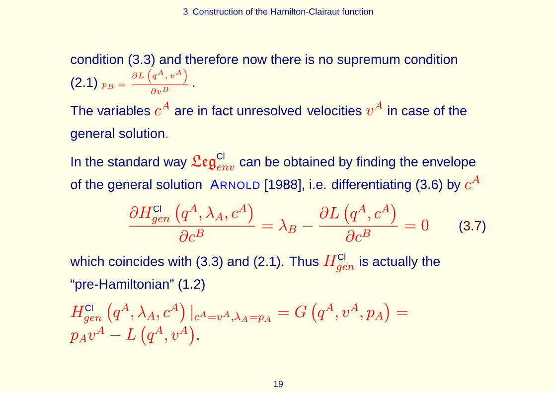
condition (3.3) and therefore now there is no supremum condition
(2.1) pB =∂L(qA, vA
)
∂vB.
The variables cA are in fact unresolved velocities vA in case of the
general solution.
In the standard way LegClenv can be obtained by finding the envelope
of the general solution ARNOLD [1988], i.e. differentiating (3.6) by cA
∂HClgen
(qA, λA, c
A)
∂cB= λB −
∂L(qA, cA
)
∂cB= 0 (3.7)
which coincides with (3.3) and (2.1). ThusHClgen is actually the
“pre-Hamiltonian” (1.2)
HClgen
(qA, λA, c
A)|cA=vA,λA=pA = G
(qA, vA, pA
)=
pAvA − L
(qA, vA
).
19

4 The mixed Legendre-Clairaut transform
4 The mixed Legendre-Clairaut transform
Consider a degenerate Lagrangian theory
L(qA, vA
)= Ldeg
(qA, vA
)for which the Hessian is zero (3.1).
The rank of Hessian matrixWAB =∂2L(qA,vA)∂vB∂vC
is r < n, and we
suppose that r is constant. We rearrange indices ofWAB in such a
way that a nonsingular minor of rank r appears in the upper left
corner GITMAN AND TYUTIN [1990]. Represent the index A as
follows: if A = 1, . . . , r, we replace A with i (the “regular” Latin
index), and, if A = r + 1, . . . , n we replace A with α (the
“degenerate” Greek index).
Obviously, detWij 6= 0, and rankWij = r.
20
4 The mixed Legendre-Clairaut transform
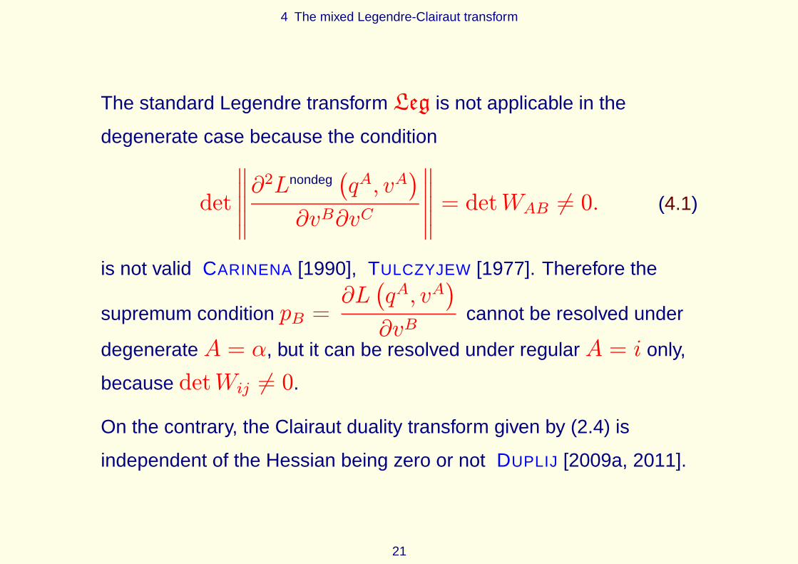
The standard Legendre transform Leg is not applicable in the
degenerate case because the condition
det
∥∥∥∥∥∂2Lnondeg
(qA, vA
)
∂vB∂vC
∥∥∥∥∥= detWAB 6= 0. (4.1)
is not valid CARINENA [1990], TULCZYJEW [1977]. Therefore the
supremum condition pB =∂L(qA, vA
)
∂vBcannot be resolved under
degenerate A = α, but it can be resolved under regular A = i only,
because detWij 6= 0.
On the contrary, the Clairaut duality transform given by (2.4) is
independent of the Hessian being zero or not DUPLIJ [2009a, 2011].
21

4 The mixed Legendre-Clairaut transform
Main idea:
The ordinary duality can be generalized to the Clairaut duality .
The standard Legendre transform Leg as
H(qA, pA
)= pBV
B(qA, pA
)− L
(qA, V A
(qA, pA
))(4.2)
can be generalized to the degenerate Lagrangian theory using the
Legendre-Clairaut transform LegCl given by the multidimensional
Clairaut equation (2.4)
H(qA, λA
)= λB
∂H(qA, λA
)
∂λB−L
(
qA,∂H
(qA, λA
)
∂λA
)
(4.3)
with λA = pA at least for some A.
22

4 The mixed Legendre-Clairaut transform
We differentiate (2.4) by λA and split the sum (3.2) in B as follows[
λi −∂L(qA, vA
)
∂vi
]
∙∂2HCl
(qA, λA
)
∂λi∂λC
+
[
λα −∂L(qA, vA
)
∂vα
]
∙∂2HCl
(qA, λA
)
∂λα∂λC= 0. (4.4)
As detWij 6= 0, we suggest to replace (4.4) by the conditions
λi = pi =∂L(qA, vA
)
∂vi, (4.5)
∂2HCl(qA, λA
)
∂λα∂λC= 0. (4.6)
23

4 The mixed Legendre-Clairaut transform
In this way we obtain a mixed envelope/general solution of the Clairaut
equation DUPLIJ [2009a, 2011, 2014]. After resolving (4.5) under
regular velocities vi = V i(qA, pi, c
α)
and writing down a solution of
(4.6) as∂HCl
(qA, λA
)
∂λα= cα (where cα being actually unresolved
velocities vα) we obtain a mixed Hamilton-Clairaut function
HClmix
(qA, pi, λα, v
α)= piV
i(qA, pi, v
α)
+ λαvα − L
(qA, V i
(qA, pi, v
α), vα), (4.7)
which is the “mixed” Legendre-Clairaut transform LLegCl
mix7−→ HClmix . a
aNote that (4.7) coincides with the “slow and careful Legendre transformation” of
TULCZYJEW AND URBANSKI [1999] and with the “generalized Legendre
transformation” of CENDRA ET AL. [1998].
24
4 The mixed Legendre-Clairaut transform
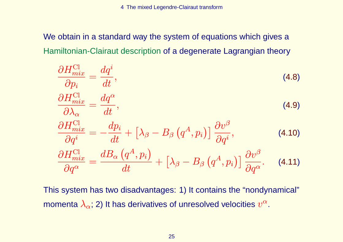
We obtain in a standard way the system of equations which gives a
Hamiltonian-Clairaut description of a degenerate Lagrangian theory
∂HClmix∂pi
=dqi
dt, (4.8)
∂HClmix∂λα
=dqα
dt, (4.9)
∂HClmix∂qi
= −dpi
dt+[λβ − Bβ
(qA, pi
)] ∂vβ
∂qi, (4.10)
∂HClmix∂qα
=dBα
(qA, pi
)
dt+[λβ − Bβ
(qA, pi
)] ∂vβ
∂qα. (4.11)
This system has two disadvantages: 1) It contains the “nondynamical”
momenta λα; 2) It has derivatives of unresolved velocities vα.
25

4 The mixed Legendre-Clairaut transform
To get rid of them, we introduce a “physical” Hamiltonian
Hphys(qA, pi
)= HClmix
(qA, pi, λα, v
α)−[λβ − Bβ
(qA, pi
)]vβ.
(4.12)
We can rewrite the “physical” Hamiltonian (4.12) using (4.7) as
Hphys(qA, pi
)= piV
i(qA, pi, v
α)
+Bα(qA, pi
)vα − L
(qA, V i
(qA, pi, v
α), vα), (4.13)
Using (4.5), we see that the r.h.s. of (4.12) indeed doesn’t depend on
“nondynamical” momenta λα and degenerate velocities vα, such that
∂Hphys
∂vα= 0. (4.14)
26

4 The mixed Legendre-Clairaut transform
Finally, we obtain from (4.8)–(4.11) the sought-for system of (first
order differential) equations (the Hamilton-Clairaut system of
equations) which describes any degenerate Lagrangian theory
dqi
dt={qi, Hphys
(qA, pi
)}reg+{qi, Bβ
(qA, pi
)}reg
dqβ
dt, i = 1, . . . r
(4.15)
dpi
dt={pi, Hphys
(qA, pi
)}phys+{pi, Bβ
(qA, pi
)}phys
dqβ
dt, i = 1, . . . r
(4.16)
Fαβ(qA, pi
) dqβ
dt= DαHphys
(qA, pi
), α = r + 1, . . . , n.
(4.17)
27
4 The mixed Legendre-Clairaut transform
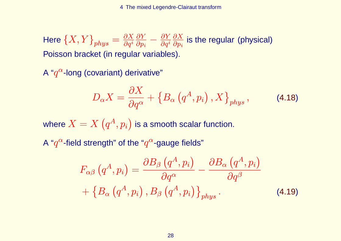
Here {X,Y }phys =∂X∂qi∂Y∂pi− ∂Y∂qi∂X∂pi
is the regular (physical)
Poisson bracket (in regular variables).
A “qα-long (covariant) derivative”
DαX =∂X
∂qα+{Bα(qA, pi
), X}phys, (4.18)
whereX = X(qA, pi
)is a smooth scalar function.
A “qα-field strength” of the “qα-gauge fields”
Fαβ(qA, pi
)=∂Bβ
(qA, pi
)
∂qα−∂Bα
(qA, pi
)
∂qβ
+{Bα(qA, pi
), Bβ
(qA, pi
)}phys. (4.19)
28
5 Nonabelian gauge theory interpretation
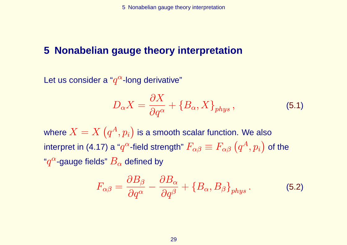
5 Nonabelian gauge theory interpretation
Let us consider a “qα-long derivative”
DαX =∂X
∂qα+ {Bα, X}phys , (5.1)
whereX = X(qA, pi
)is a smooth scalar function. We also
interpret in (4.17) a “qα-field strength” Fαβ ≡ Fαβ(qA, pi
)of the
“qα-gauge fields” Bα defined by
Fαβ =∂Bβ
∂qα−∂Bα
∂qβ+ {Bα, Bβ}phys . (5.2)
29
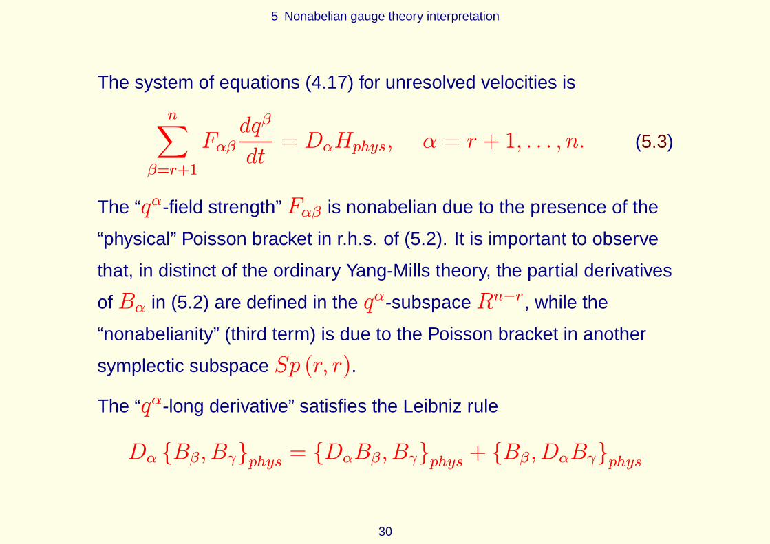
5 Nonabelian gauge theory interpretation
The system of equations (4.17) for unresolved velocities is
n∑
β=r+1
Fαβdqβ
dt= DαHphys, α = r + 1, . . . , n. (5.3)
The “qα-field strength” Fαβ is nonabelian due to the presence of the
“physical” Poisson bracket in r.h.s. of (5.2). It is important to observe
that, in distinct of the ordinary Yang-Mills theory, the partial derivatives
of Bα in (5.2) are defined in the qα-subspace Rn−r, while the
“nonabelianity” (third term) is due to the Poisson bracket in another
symplectic subspace Sp (r, r).
The “qα-long derivative” satisfies the Leibniz rule
Dα {Bβ, Bγ}phys = {DαBβ, Bγ}phys + {Bβ, DαBγ}phys
30

5 Nonabelian gauge theory interpretation
which is valid while acting on “qα-gauge fields” Bα. The commutator
of the “qα-long derivatives” is now equal to the Poisson bracket with
the “qα-field strength”
(DαDβ −DβDα)X = {Fαβ, X}phys . (5.4)
It follows from (5.4)
DαDβFαβ = 0. (5.5)
31

5 Nonabelian gauge theory interpretation
Let us introduce the Bα-transformation
δBαX = {Bα, X}phys , (5.6)
which satisfies
(δBαδBβ − δBβδBα
)Bγ = δ{Bα,Bβ}
phys
Bγ, (5.7)
δBαFβγ(qA, pi
)= (DγDβ −DβDγ)Bα, (5.8)
δBα {Bβ, Bγ}phys = {δBαBβ, Bγ}phys + {Bβ, δBαBγ}phys .
(5.9)
This means that the “qα-long derivative”Dα (4.18) is in fact a
“qα-covariant derivative” with respect to the Bα-transformation (5.6).
32
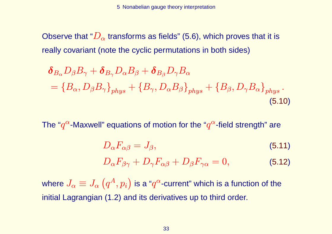
5 Nonabelian gauge theory interpretation
Observe that “Dα transforms as fields” (5.6), which proves that it is
really covariant (note the cyclic permutations in both sides)
δBαDβBγ + δBγDαBβ + δBβDγBα
= {Bα, DβBγ}phys + {Bγ, DαBβ}phys + {Bβ, DγBα}phys .
(5.10)
The “qα-Maxwell” equations of motion for the “qα-field strength” are
DαFαβ = Jβ, (5.11)
DαFβγ +DγFαβ +DβFγα = 0, (5.12)
where Jα ≡ Jα(qA, pi
)is a “qα-current” which is a function of the
initial Lagrangian (1.2) and its derivatives up to third order.
33

5 Nonabelian gauge theory interpretation
Due to (5.5) the “qα-current” Jα is conserved
DαJα = 0. (5.13)
Thus, a singular Lagrangian system leads effectively to some special
kind of the nonabelian gauge theory in the direct product space
Mphys = Rn−r × Sp (r, r). Here the “nonabelianity” (third term in
(5.2)) appears not due to a Lie algebra (as in the Yang-Mills theory),
but “classically”, due to the Poisson bracket in the symplectic
subspace Sp (r, r). The corresponding manifold can be interpreted
locally as a special kind of the degenerate Poisson manifold (see, e.g.,
BUEKEN [1996]).
34

5 Nonabelian gauge theory interpretation
The analogous Poisson type of “nonabelianity” (5.2) appears in the
N →∞ limit of Yang-Mills theory, and it is called the “Poisson gauge
theory” FLORATOS ET AL. [1989]. In the SU (∞) Yang-Mills theory
the group indices become surface coordinates FAIRLIE ET AL. [1990],
and it is connected with the Schild string ZACHOS [1990]. The related
algebra generalizations are called the continuum graded Lie algebras
SAVELIEV AND VERSHIK [1990]. Here, because of the direct product
structure of the spaceMphys, the similar construction appears in
(5.2), while the “long derivative” (4.18), “gauge transformations” (5.6)
and the analog of the Maxwell equations (5.11)–(5.12) differ from the
“Poisson gauge theory” FLORATOS ET AL. [1989].
Some applications of the presented formalism for two-color QCD was
recently done in WALKER AND DUPLIJ [2015] (Phys. Rev. D).
35
6 Partial Hamiltonian formalism
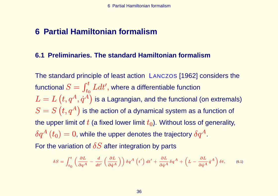
6 Partial Hamiltonian formalism
6.1 Preliminaries. The standard Hamiltonian formalism
The standard principle of least action LANCZOS [1962] considers the
functional S =∫ tt0Ldt′, where a differentiable function
L = L(t, qA, qA
)is a Lagrangian, and the functional (on extremals)
S = S(t, qA
)is the action of a dynamical system as a function of
the upper limit of t (a fixed lower limit t0). Without loss of generality,
δqA (t0) = 0, while the upper denotes the trajectory δqA.
For the variation of δS after integration by parts
δS =
∫t
t0
(∂L
∂qA−d
dt′
(∂L
∂qA
))δqA(t′)dt′+∂L
∂qAδqA+
(L−
∂L
∂qAqA)δt, (6.1)
36

6 Partial Hamiltonian formalism
Then, from δS = 0, we obtain the equations of motion
(Euler-Lagrange equations) LANDAU AND LIFSHITZ [1969]
∂L
∂qA−d
dt
(∂L
∂qA
)
= 0 A = 1, . . . , n. (6.2)
The second and third terms in (6.1) define the total differential of the
action (on extremals) as a function of (n+ 1) variables: the
coordinates and the upper limit of integration in (6.1)
dS =∂L
∂qAdqA +
(
L−∂L
∂qAqA)
dt. (6.3)
Thus, from the definition of the action (6.1) and (6.3), it follows thatdS
dt= L,
∂S
∂qA=∂L
∂qA,∂S
∂t= L−
∂L
∂qAqA. In the standard
Hamiltonian formalism LANDAU AND LIFSHITZ [1969], to each
37

6 Partial Hamiltonian formalism
coordinate qA one can assign the canonically conjugate momentum
pA by the formula
pA =∂L
∂qA, A = 1, . . . , n. (6.4)
If the system of equations (6.4) is solvable for all velocities qA, we can
define the Hamiltonian by the Legendre transform LANDAU AND
LIFSHITZ [1969]
H = pAqA − L, (6.5)
which defines the mapping TQ∗n → TQn ARNOLD [1989].
The r.h.s. of (6.5) is expressed in terms of the momenta, so that
H = H(t, qA, pA
)is a function on the phase space (or the
cotangent bundle TQ∗n of rank n and the dimension of the total space
38

6 Partial Hamiltonian formalism
2n), that is independent of 2n canonical coordinates(qA, pA
). In the
standard canonical formalism, each coordinate qA has its conjugate
momentum pA by the formula (6.4), we call it a full Hamiltonian
formalism (in the full phase space TQ∗n). Then the differential of the
action (6.3) can also be written as
dS = pAdqA −Hdt. (6.6)
∂S
∂qA= pA,
∂S
∂t= −H
(t, qA, pA
), (6.7)
The Hamilton-Jacobi differential equation
∂S
∂t+H
(
t, qA,∂S
∂qA
)
= 0, (6.8)
which determines the dynamics in terms ofH(t, qA, pA
).
39

6 Partial Hamiltonian formalism
Variation of the action S =∫ (pAdq
A −Hdt)
while considering the
coordinates and momenta as independent variables, gives the
Hamilton’s equations in the differential form LANDAU AND LIFSHITZ
[1969] to
dqA =∂H
∂pAdt, dpA = −
∂H
∂qAdt (6.9)
for the full Hamiltonian formalism.
40

6 Partial Hamiltonian formalism
In terms of the (full) Poisson bracket
{A,B}full =∂A
∂qA∂B
∂pA−∂B
∂qA∂A
∂pA(6.10)
(6.9) can be written in standard form LANDAU AND LIFSHITZ [1969]
dqA ={qA, H
}fulldt, dpA = {pA, H}full dt. (6.11)
It is clear that the two formulations of the principle of the least action,
that is (6.1) and (6.1), are completely equivalent. Now we will show in
this simple language, how to describe the same dynamics using fewer
generalized momenta than the number of generalized coordinates.
41

6 Partial Hamiltonian formalism
6.2 Hamiltonian formalism with reduced number of momenta
The transition from a full to a partial Hamiltonian formalism and a
multi-time dynamics can be analyzed using the following well-known
classical analogy LANCZOS [1962], but in its reverse form. Recall, the
extended phase space with the following additional position and
momentum
qn+1 = t, (6.12)
pn+1 = −H. (6.13)
42

6 Partial Hamiltonian formalism
Then the action (6.1) takes the symmetrical form and contains only
the first term LANCZOS [1962] (see, also ARNOWITT ET AL. [1962])
S =
∫ n+1∑
A=1
pAdqA. (6.14)
Here we proceed in the opposite way, and ask: can we, on the
contrary, not increase, but reduce the number of momenta that
describe the dynamical system? Can we formulate a version of
so-called partial Hamiltonian formalism, which would be equivalent (at
the classical level) to the Lagrangian formalism?
The answer is: Yes.
43

6 Partial Hamiltonian formalism
We define a partial Hamiltonian formalism DUPLIJ [2013, 2015], so
that the conjugate momentum is associated not to every qA by the
formula (6.4), but only for the first np < n generalized coordinates,
which are called canonical and denoted by qi, i = 1, . . . np. The
resulting tangent bundle TQ∗np is defined by 2np (reduced) canonical
coordinates (qi, pi). The rest of the generalized coordinates are
called noncanonical qα, α = np + 1, . . . n, and they form a
configuration subspaceQn−np , which corresponds to the tangent
bundle TQn−np (a subscript indicates the corresponding dimension
of the total space). Thus, the dynamical system is now given on the
direct product (of manifolds) TQ∗np × TQn−np .
44
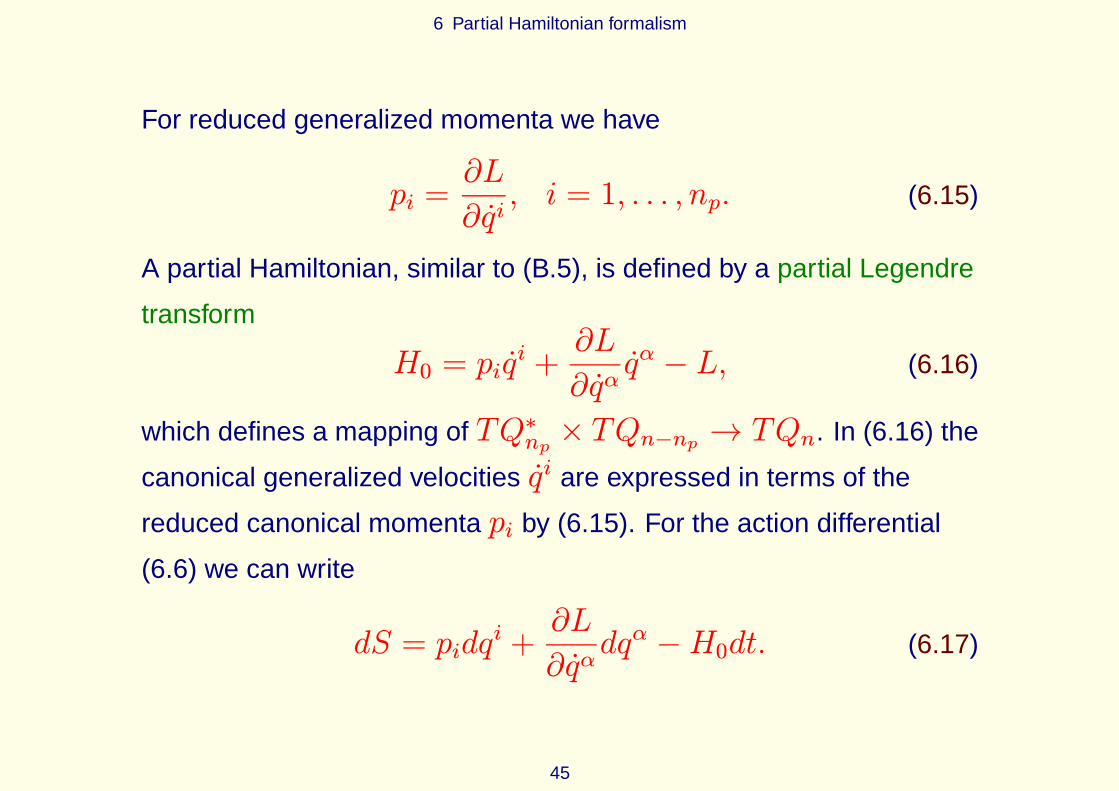
6 Partial Hamiltonian formalism
For reduced generalized momenta we have
pi =∂L
∂qi, i = 1, . . . , np. (6.15)
A partial Hamiltonian, similar to (B.5), is defined by a partial Legendre
transform
H0 = piqi +∂L
∂qαqα − L, (6.16)
which defines a mapping of TQ∗np × TQn−np → TQn. In (6.16) the
canonical generalized velocities qi are expressed in terms of the
reduced canonical momenta pi by (6.15). For the action differential
(6.6) we can write
dS = pidqi +∂L
∂qαdqα −H0dt. (6.17)
45

6 Partial Hamiltonian formalism
We define
Hα = −∂L
∂qα, α = np + 1, . . . n (6.18)
dS = pidqi −Hαdq
α −H0dt. (6.19)
Without the second term in (6.19) the partial Hamiltonian (6.16) is the Routh function in terms of which the Lagrange equations of motion
can be reformulated LANDAU AND LIFSHITZ [1969].
In the partial Hamiltonian formalism the dynamics is completely
determined by the set of (n− np + 1) HamiltoniansH0,Hα,
α = np + 1, . . . n.
46
and call them additional Hamiltonians (note H α = −B α )

6 Partial Hamiltonian formalism
It follows from (6.19) that the partial derivatives of S = S (t, qi, qα)
are ∂S
∂qi= pi,
∂S
∂qα= −Hα
(t, qi, pi, q
α, qα),∂S
∂t= −H0
(t, qi, pi, q
α, qα), which
yields the system (n− np + 1) of Hamilton-Jacobi equations
∂S
∂t+H0
(
t, qi,∂S
∂qi, qα, qα
)
= 0, (6.20)
∂S
∂qα+Hα
(
t, qi,∂S
∂qi, qα, qα
)
= 0. (6.21)
Now, on the direct product of TQ∗np × TQn−np , the action is
S =
∫ (pidq
i −Hαdqα −H0dt
). (6.22)
Variation of (6.22) should be made independently on 2np-reduced
coordinates qi, pi and (n− np) noncanonical coordinates qα.
47

6 Partial Hamiltonian formalism
The equations of motion for the partial Hamiltonian formalism can be
derived from δS = 0. We introduce the reduced Poisson bracket for
two functions A and B in the reduced phase space TQ∗np
{A,B} =∂A
∂qi∂B
∂pi−∂B
∂qi∂A
∂pi. (6.23)
48

6 Partial Hamiltonian formalism
The equations of motion on TQ∗np × TQn−np in the differential form
dqi ={qi, H0
}dt+
{qi, Hβ
}dqβ, (6.24)
dpi = {pi, H0} dt+ {pi, Hβ} dqβ, (6.25)
∂Hα
∂qβdqβ +
d
dt
(∂H0
∂qα+∂Hβ
∂qαqβ)
dt =
(∂Hβ
∂qα−∂Hα
∂qβ+ {Hβ, Hα}
)
dqβ
+
(∂H0
∂qα−∂Hα
∂t+ {H0, Hα}
)
dt. (6.26)
On TQ∗np the first-order equations (6.24)–(6.25). On (noncanonical)
subspace TQn−np the equation (6.26) is still of second order.
49
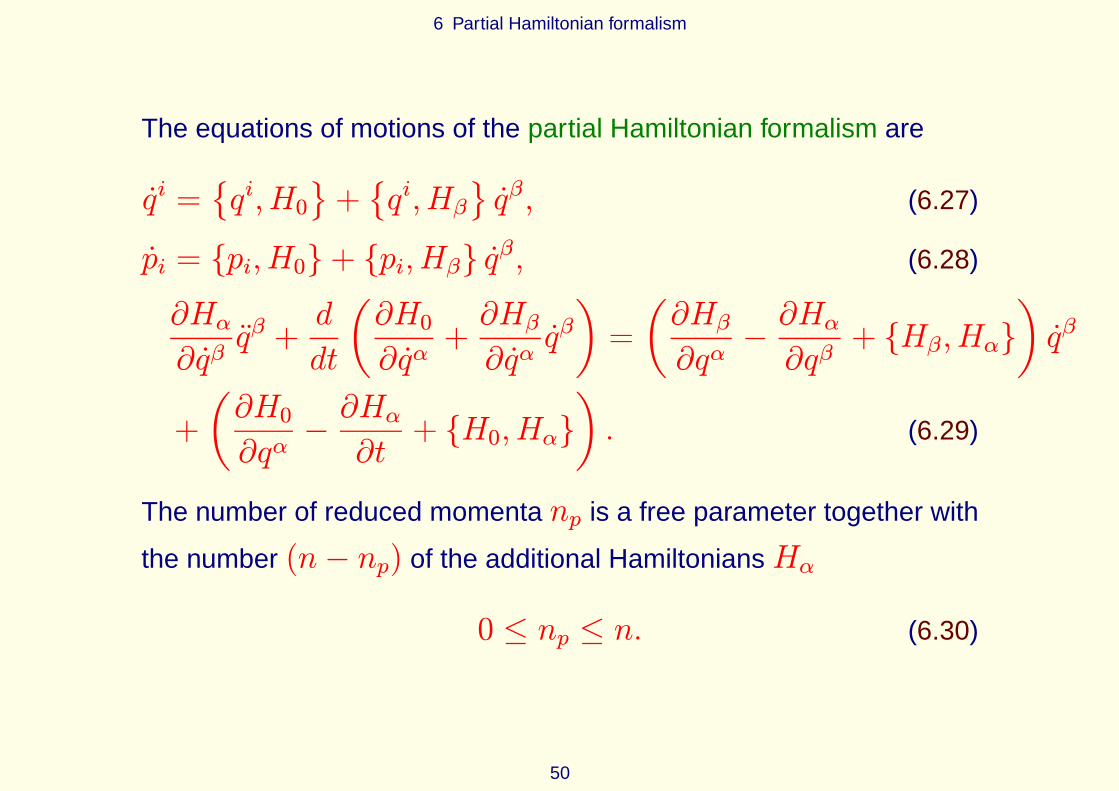
6 Partial Hamiltonian formalism
The equations of motions of the partial Hamiltonian formalism are
qi ={qi, H0
}+{qi, Hβ
}qβ, (6.27)
pi = {pi, H0}+ {pi, Hβ} qβ, (6.28)
∂Hα
∂qβqβ +
d
dt
(∂H0
∂qα+∂Hβ
∂qαqβ)
=
(∂Hβ
∂qα−∂Hα
∂qβ+ {Hβ, Hα}
)
qβ
+
(∂H0
∂qα−∂Hα
∂t+ {H0, Hα}
)
. (6.29)
The number of reduced momenta np is a free parameter together with
the number (n− np) of the additional HamiltoniansHα
0 ≤ np ≤ n. (6.30)
50

6 Partial Hamiltonian formalism
In other words, the dynamics is independent of the dimension of the
reduced phase space. In this case, the boundary values of np
correspond to the standard Lagrangian and Hamiltonian formalisms,
respectively, so that we have the three cases:
1. np = 0— the Lagrangian formalism on TQn (we have only the
last equation (6.29) without the Poisson brackets), and
α = 1, . . . , n;
2. 0 < np < n— the partial Hamiltonian formalism for
TQ∗np × TQn−np (all of the equations are considered);
3. np = n— the standard Hamiltonian formalism on TQ∗n (the first
two equations (6.27 )–(6.28) without the second terms, coinciding
with the standard Hamiltonian equations (6.9), i = 1, . . . , n.
51

6 Partial Hamiltonian formalism
We can show that in the case 1) we obtain the standard Lagrange
equations for the noncanonical variables qα. We derive from (4.9)
d
dt
∂
∂qα(H0 +Hβ q
β)=∂
∂qα(H0 +Hβ q
β). (6.31)
The formula to determine the partial Hamiltonian (6.16) without
variables qi, pi is
H0 = −Hαqα − L. (6.32)
Hence,H0 +Hβ qβ = −L, we obtain the standard Lagrange
equations in the noncanonical sector
d
dt
∂
∂qαL =
∂
∂qαL. (6.33)
52

6 Partial Hamiltonian formalism
A non-trivial dynamics in the noncanonical sector is determined by the
presence of terms with second derivatives. Consider a special case of
the partial Hamiltonian formalism, when these terms (with second
derivatives) vanish and call it nondynamical in the noncanonical sector
(because, there are no noncanonical accelerations qα). This requires
∂H0
∂qβ= 0,
∂Hα
∂qβ= 0, α, β = np + 1, . . . , n. (6.34)
Then (6.29) will have only the right side, which can be written as(∂Hβ
∂qα−∂Hα
∂qβ+ {Hβ, Hα}
)
qβ = −
(∂H0
∂qα−∂Hα
∂t+ {H0, Hα}
)
,
(6.35)
which is a system of linear algebraic equations for the noncanonical
velocities qα with the given HamiltoniansH0,Hα.
53
7 Singular theories in partial Hamiltonian formalism
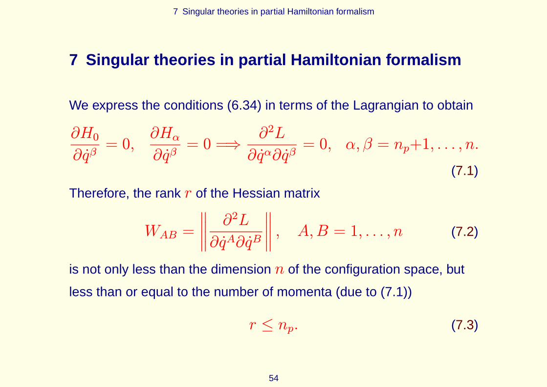
7 Singular theories in partial Hamiltonian formalism
We express the conditions (6.34) in terms of the Lagrangian to obtain
∂H0
∂qβ= 0,
∂Hα
∂qβ= 0 =⇒
∂2L
∂qα∂qβ= 0, α, β = np+1, . . . , n.
(7.1)
Therefore, the rank r of the Hessian matrix
WAB =
∥∥∥∥∂2L
∂qA∂qB
∥∥∥∥ , A,B = 1, . . . , n (7.2)
is not only less than the dimension n of the configuration space, but
less than or equal to the number of momenta (due to (7.1))
r ≤ np. (7.3)
54

7 Singular theories in partial Hamiltonian formalism
The definition of “extra ” (np − r) momenta results in a (np − r)
relations, just as in the Dirac theory of constraints DIRAC [1964].
1) In the standard Hamiltonian formalism there are exactly (n− r)
constraints, because the dimension n of the configuration space
(np = n) and rank of the Hessian r are fixed by the problem.
2) In the partial Hamiltonian formalism the number np of momenta is
a free parameter that can be chosen so that the constraints do not
appear i.e. (np − r) = 0. Thus, to describe singular theories without
using constraints it is natural to equate the number of momenta with
the rank of the Hessian
np = r. (7.4)
55

7 Singular theories in partial Hamiltonian formalism
Main idea. The singular dynamics (theory with degenerate
Lagrangian) can be formulated in a way that constraints will not occur.
In the Hessian matrixWAB (7.2) we rename the indices so that the
non-singular minor rank r is in the upper left hand corner, denote with
the Latin alphabet i, j the first r indices and with Greek letters α, β
the remaining (n− r) indices. The equations of motion are
qi ={qi, H0
}+{qi, Hβ
}qβ, (7.5)
pi = {pi, H0}+ {pi, Hβ} qβ, (7.6)
Fαβ qβ = Gα, (7.7)
where nowH0 = Hphys and { } becomes { }phys.
56

7 Singular theories in partial Hamiltonian formalism
Here the index values are connected with the rank of the Hessian by
i = 1, . . . , r, α, β = r + 1, . . . , n, and
Fαβ =∂Hα
∂qβ−∂Hβ
∂qα+ {Hα, Hβ} , (7.8)
Gα = DαH0 =∂H0
∂qα−∂Hα
∂t+ {H0, Hα} . (7.9)
The system of equations (7.5 )–(7.9) coincides with the equations
derived in the approach to singular theories (4.15 )–(4.17), which uses
the mixed solutions of Clairaut’s equation DUPLIJ [2009b, 2011]
(except for the term with the partial time derivative ofHα in (7.9)).
57

8 Classification, gauge freedom and new brackets
8 Classification, gauge freedom and new brackets
Next we classify degenerate Lagrangian theories as follows. There
are two possibilities determined by the rank of the matrix Fαβ :
1. Nongauge theory, when rankFαβ = rF = n− r is full, so that
the matrix Fαβ is invertible. Then
qα = F αβGβ, (8.1)
where F αβ is the inverse matrix of Fαβ , defined by the equation
F αβFβγ = FγβFβα = δαγ .
2. Gauge theory, the rank of the Fαβ is incomplete, that is,
rF < n− r, and the matrix Fαβ is noninvertible.
58
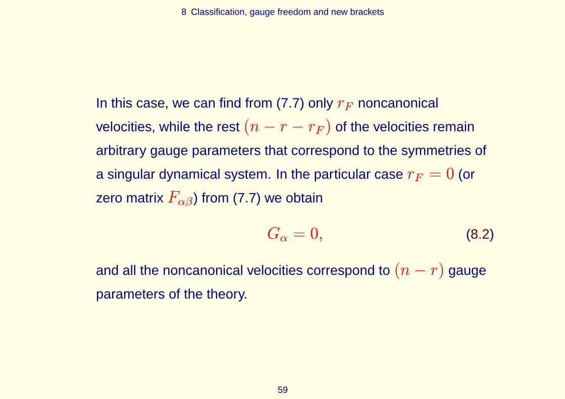
8 Classification, gauge freedom and new brackets
In this case, we can find from (7.7) only rF noncanonical
velocities, while the rest (n− r − rF ) of the velocities remain
arbitrary gauge parameters that correspond to the symmetries of
a singular dynamical system. In the particular case rF = 0 (or
zero matrix Fαβ) from (7.7) we obtain
Gα = 0, (8.2)
and all the noncanonical velocities correspond to (n− r) gauge
parameters of the theory.
59

8 Classification, gauge freedom and new brackets
In the first case all the noncanonical velocities can be excluded and
the Hamilton-like equations for nongauge singular systems
qi ={qi, H0
}nongauge
, (8.3)
pi = {pi, H0}nongauge , (8.4)
where a new (nongauge) bracket for A,B is
{A,B}nongauge = {A,B}+DαA ∙ Fαβ ∙DβB, (8.5)
andDα is defined in (7.9). The nongauge bracket (8.5) uniquely
determines the evolution of any dynamical quantity A in time
dA
dt=∂A
∂t+ {A,H0}nongauge . (8.6)
60

8 Classification, gauge freedom and new brackets
The nongauge bracket (8.5) has all the properties of the Poisson
bracket: it is antisymmetric and satisfies the Jacobi identity.
In the second case (gauge theory), only some of the noncanonical
velocities qα can be eliminated, the number of which is equal to the
rank rF of the matrix Fαβ , and the rest (n− r − rF ) of the
velocities are still arbitrary and can serve as gauge parameters. Then
in the system (7.7), only the first rF equations are independent. We
present (“noncanonical”) indices α, β = r + 1, . . . , n as pairs
(α1, α2), (β1, β2), where α1, β1 = r + 1, . . . , rF number the first
rF independent rows of the matrix Fαβ and correspond to the
nonsingular minor of Fα1β1 , the remaining (n− r − rF ) rows will be
dependent on the first ones, and α2, β2 = rF + 1, . . . , n.
61
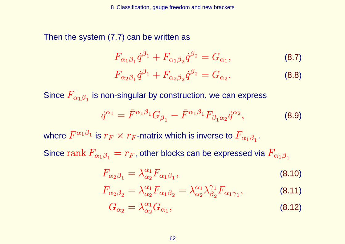
8 Classification, gauge freedom and new brackets
Then the system (7.7) can be written as
Fα1β1 qβ1 + Fα1β2 q
β2 = Gα1 , (8.7)
Fα2β1 qβ1 + Fα2β2 q
β2 = Gα2 . (8.8)
Since Fα1β1 is non-singular by construction, we can express
qα1 = F α1β1Gβ1 − Fα1β1Fβ1α2 q
α2 , (8.9)
where F α1β1 is rF × rF -matrix which is inverse to Fα1β1 .
Since rankFα1β1 = rF , other blocks can be expressed via Fα1β1
Fα2β1 = λα1α2Fα1β1 , (8.10)
Fα2β2 = λα1α2Fα1β2 = λ
α1α2λγ1β2Fα1γ1 , (8.11)
Gα2 = λα1α2Gα1 , (8.12)
62
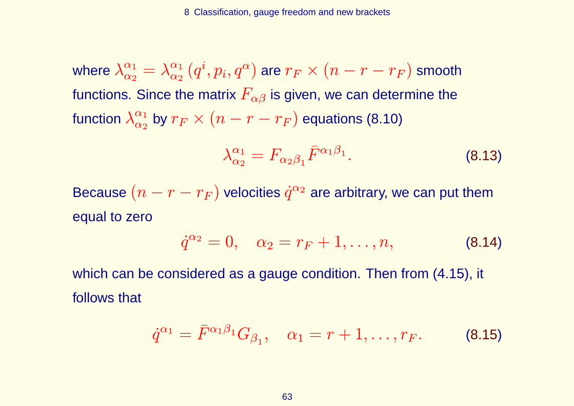
8 Classification, gauge freedom and new brackets
where λα1α2 = λα1α2(qi, pi, q
α) are rF × (n− r − rF ) smooth
functions. Since the matrix Fαβ is given, we can determine the
function λα1α2 by rF × (n− r − rF ) equations (8.10)
λα1α2 = Fα2β1Fα1β1 . (8.13)
Because (n− r − rF ) velocities qα2 are arbitrary, we can put them
equal to zero
qα2 = 0, α2 = rF + 1, . . . , n, (8.14)
which can be considered as a gauge condition. Then from (4.15), it
follows that
qα1 = F α1β1Gβ1 , α1 = r + 1, . . . , rF . (8.15)
63
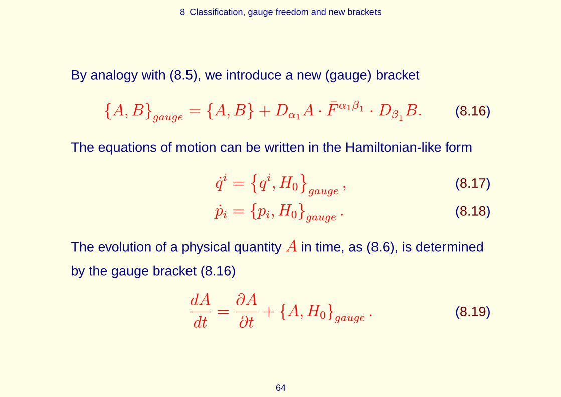
8 Classification, gauge freedom and new brackets
By analogy with (8.5), we introduce a new (gauge) bracket
{A,B}gauge = {A,B}+Dα1A ∙ Fα1β1 ∙Dβ1B. (8.16)
The equations of motion can be written in the Hamiltonian-like form
qi ={qi, H0
}gauge
, (8.17)
pi = {pi, H0}gauge . (8.18)
The evolution of a physical quantity A in time, as (8.6), is determined
by the gauge bracket (8.16)
dA
dt=∂A
∂t+ {A,H0}gauge . (8.19)
64

8 Classification, gauge freedom and new brackets
In the particular case, when rF = 0, we have
Fαβ = 0, (8.20)
and hence all additional Hamiltonians vanishHα = 0, then it is seen
from the definition (6.18) that the Lagrangian does not depend on the
noncanonical velocities qα. Therefore, taking into account (8.20) and
(7.7) we find that the partial HamiltonianH0 does not depend on the
noncanonical generalized coordinates qα
∂H0
∂qα= 0, (8.21)
ifH0 is manifestly independent of time. In this case, the gauge
bracket coincides with the Poisson bracket, since the second term in
(8.16) vanishes.
65

9 Singular theory as multi-time dynamics
9 Singular theory as multi-time dynamics
The conditions (6.34) ∂H0∂qβ
= 0,∂Hα
∂qβ= 0 mean that all the Hamiltonians
in the partial Hamiltonian formalism do not depend on the velocities
qα, that is,H0 = H0 (t, qi, pi, q
α),Hα = Hα (t, qi, pi, q
α),
i = 1, . . . , np, α = np + 1, . . . , n. Thus, the dynamical problem is
defined on the manifold TQ∗np ×Qn−np , so that qα actually play the
role of real parameters, similar to the time. In this case the
nondynamicalQn−np is isomorphic to the real space Rn−np .
66

9 Singular theory as multi-time dynamics
Therefore, we can interpret (n− np) canonical generalized
coordinates qα as (n− np) “extra” (to t) times, andHα as (n− np)corresponding Hamiltonians. Indeed, we introduce DUPLIJ [2015]
τμ = t, Hμ = H0, μ = 0, (9.1)
τμ = qμ+np , Hμ = Hμ+np , μ = 1, . . . , (n− np) , (9.2)
where Hμ = Hμ (τμ, qi, pi) are Hamiltonians of the multi-time
dynamics with nμ = n− np + 1 times τμ. Note that τμ can be
called generalized times, because they are not real times (for the real
multi-time physics see DORLING [1970], DVALI ET AL. [2000] and
review BARS AND TERNING [2010]), in the same way as generalized
coordinates have nothing to do with space-time coordinates LANDAU
AND LIFSHITZ [1969].
67
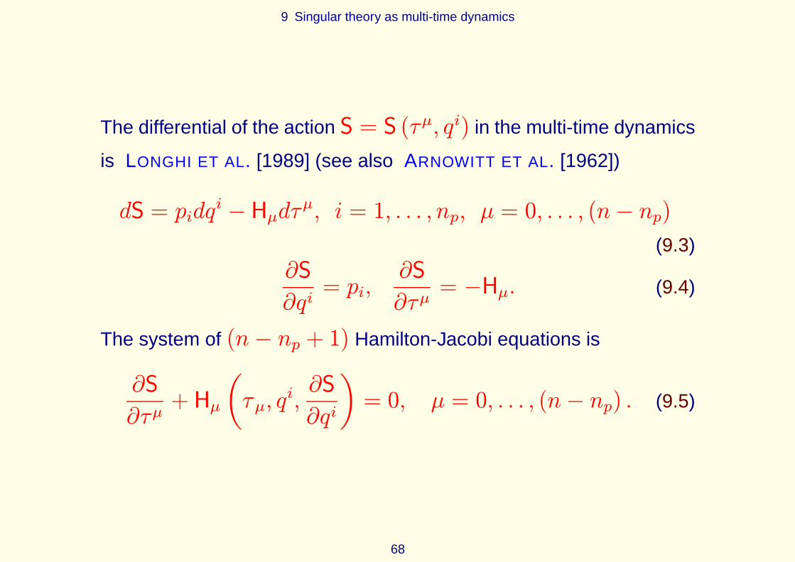
9 Singular theory as multi-time dynamics
The differential of the action S = S (τμ, qi) in the multi-time dynamics
is LONGHI ET AL. [1989] (see also ARNOWITT ET AL. [1962])
dS = pidqi − Hμdτ
μ, i = 1, . . . , np, μ = 0, . . . , (n− np)
(9.3)∂S
∂qi= pi,
∂S
∂τμ= −Hμ. (9.4)
The system of (n− np + 1) Hamilton-Jacobi equations is
∂S
∂τμ+ Hμ
(
τμ, qi,∂S
∂qi
)
= 0, μ = 0, . . . , (n− np) . (9.5)
68
9 Singular theory as multi-time dynamics
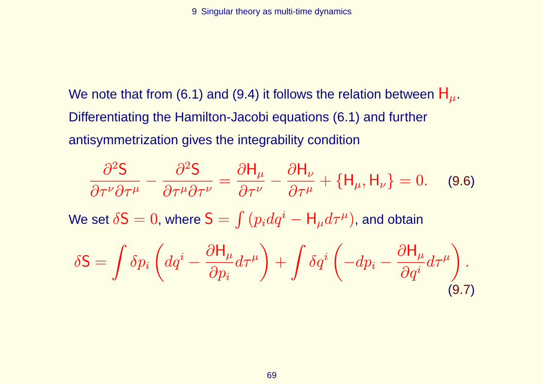
We note that from (6.1) and (9.4) it follows the relation between Hμ.
Differentiating the Hamilton-Jacobi equations (6.1) and further
antisymmetrization gives the integrability condition
∂2S
∂τ ν∂τμ−∂2S
∂τμ∂τ ν=∂Hμ∂τ ν−∂Hν∂τμ+ {Hμ,Hν} = 0. (9.6)
We set δS = 0, where S =∫(pidq
i − Hμdτμ), and obtain
δS =
∫δpi
(
dqi −∂Hμ∂pidτμ)
+
∫δqi(
−dpi −∂Hμ∂qidτμ)
.
(9.7)
69

9 Singular theory as multi-time dynamics
Therefore, the equations of motion for the multi-time dynamics can be
written in differential form LONGHI ET AL. [1989]
dqi ={qi,Hμ
}dτμ, (9.8)
dpi = {pi,Hμ} dτμ, (9.9)
which coincide with (6.24)–(6.25) by construction. The integrability
conditions (9.6) can be also written in differential forma
(∂Hμ∂τ ν−∂Hν∂τμ+ {Hμ,Hν}
)
dτ ν = 0, μ, ν = 0, . . . , (n− np)
(9.10)
which coincide with the equations (6.35), written in differential form.aAs in the standard case, ARNOLD [1989], the equations (9.8 )–(9.10) are the
conditions for closure of a differential 1-form (9.3).
70
9 Singular theory as multi-time dynamics
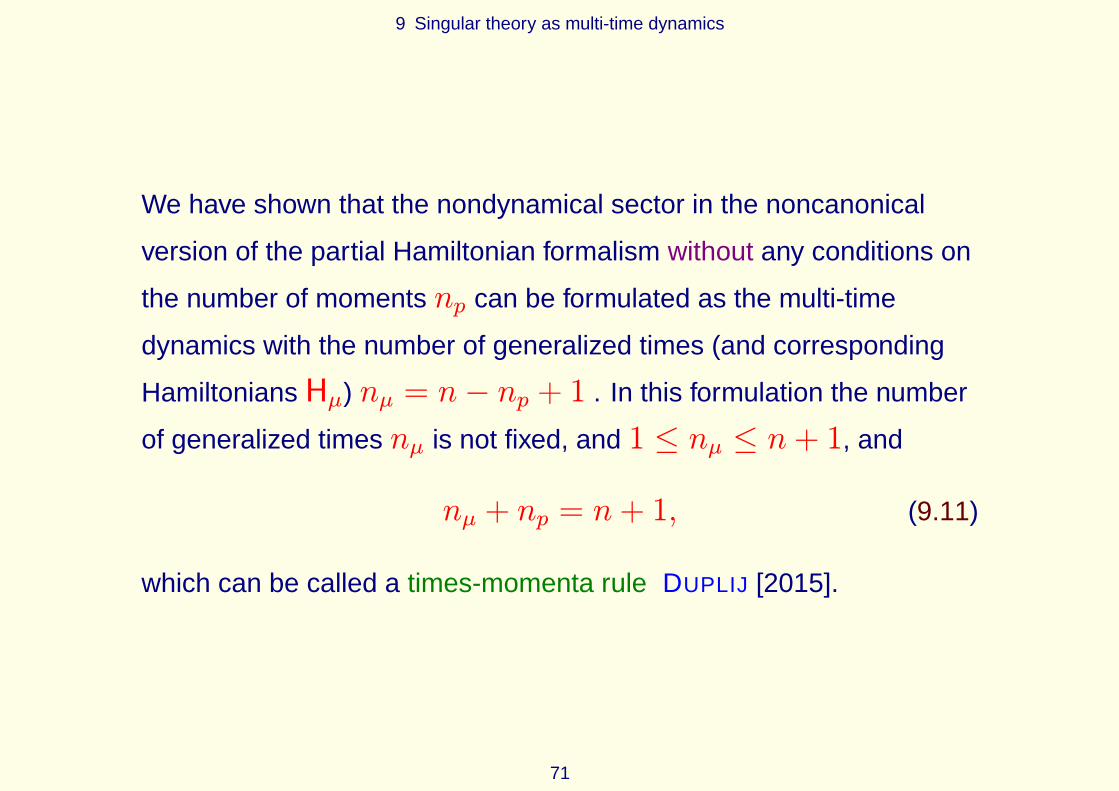
We have shown that the nondynamical sector in the noncanonical
version of the partial Hamiltonian formalism without any conditions on
the number of moments np can be formulated as the multi-time
dynamics with the number of generalized times (and corresponding
Hamiltonians Hμ) nμ = n− np + 1 . In this formulation the number
of generalized times nμ is not fixed, and 1 ≤ nμ ≤ n+ 1, and
nμ + np = n+ 1, (9.11)
which can be called a times-momenta rule DUPLIJ [2015].
71

9 Singular theory as multi-time dynamics
In the particular case of singular theories (with degenerate
Lagrangians), the number of momenta np is fixed by the condition
(7.4) np = r. From (9.11) we obtain
nμ + r = n+ 1, (9.12)
which can be called a times-rank rule DUPLIJ [2015].
Thus, a singular theory can be effectively described as the multi-time
dynamics, such that (6.34) ∂H0∂qβ
= 0,∂Hα
∂qβ= 0 and (9.12) are fulfilled.
72

10 Origin of constraints in singular theories
10 Origin of constraints in singular theories
Introduction of additional dynamical variables must necessarily give
rise to additional relationships between them. Consider the “extra”
(n− r) momenta pα (since we have a complete description of the
dynamics without them), which correspond to noncanonical
generalized velocities qα for the standard definition DIRAC [1964]
pα =∂L
∂qα, α = r + 1, . . . , n. (10.1)
So (10.1), together with the definition of the partial generalized
canonical momenta (6.15) coincide with “full” momenta (6.4)
pA =∂L
∂qA, A = 1, . . . , n.
73
10 Origin of constraints in singular theories
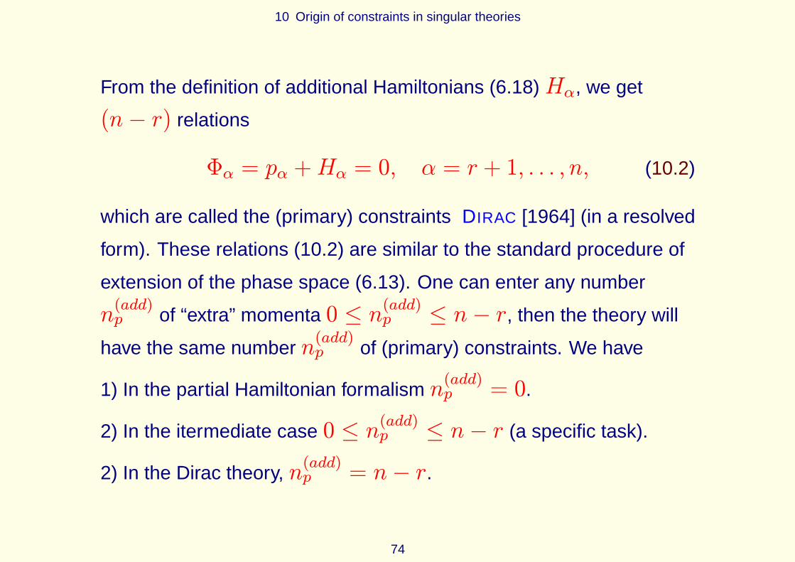
From the definition of additional Hamiltonians (6.18)Hα, we get
(n− r) relations
Φα = pα +Hα = 0, α = r + 1, . . . , n, (10.2)
which are called the (primary) constraints DIRAC [1964] (in a resolved
form). These relations (10.2) are similar to the standard procedure of
extension of the phase space (6.13). One can enter any number
n(add)p of “extra” momenta 0 ≤ n(add)p ≤ n− r, then the theory will
have the same number n(add)p of (primary) constraints. We have
1) In the partial Hamiltonian formalism n(add)p = 0.
2) In the itermediate case 0 ≤ n(add)p ≤ n− r (a specific task).
2) In the Dirac theory, n(add)p = n− r.
74

10 Origin of constraints in singular theories
If we have the “extra” momenta pα, as in Dirac approach, the
transition to the Hamiltonian by the standard formula
Htotal = piqi + pαq
α − L, (10.3)
cannot be done directly, therefore,Htotal is also not a “true”
Hamiltonian, asH0 in (6.16). It is impossible to express the
noncanonical velocities qα through the “extra” momenta pα and then
apply the standard Legendre transformation. But it is possible to
transformHtotal (10.3) in such a way that one can use the method of
undetermined coefficients DIRAC [1964]. The total Hamiltonian can
be written as
Htotal = H0 + qαΦα, (10.4)
where qα play the role of undetermined coefficients.
75

10 Origin of constraints in singular theories
The equations of motion can be written in a Hamiltonian-like form in
terms of the total HamiltonianHtotal and the full Poisson bracket
dqA ={qA, Htotal
}fulldt, (10.5)
dpA = {pA, Htotal}full dt (10.6)
with the (n− r) conditions (10.2) Φα = pα +Hα = 0.
However, the equations (10.5)–(10.6) and (10.2) are not sufficient to
solve the problem: to find the equations for the undetermined
coefficients qα in (10.4). These equations can be derived from some
additional principles, such as conservation relations (10.2) in time
DIRAC [1964]dΦαdt= 0. (10.7)
76

10 Origin of constraints in singular theories
The time dependence of any physical quantity A is now determined
by the total Hamiltonian and the full Poisson bracket
dA
dt=∂A
∂t+ {A,Htotal}full . (10.8)
If the constraints do not depend explicitly on time, then from (10.8)
and (10.4) we obtain
{Φα, Htotal}full = {Φα, H0}full + {Φα,Φβ}full qβ = 0, (10.9)
which is a system of equations for the undetermined coefficients qα.
Note that (10.9) coincides with (7.7) Fαβ qβ = Gα = DαH0, since
Fαβ = {Φα,Φβ}full , (10.10)
DαH0 = {Φα, H0}full . (10.11)
77
10 Origin of constraints in singular theories
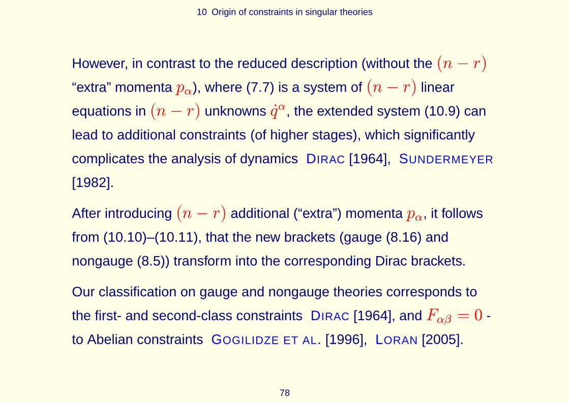
However, in contrast to the reduced description (without the (n− r)
“extra” momenta pα), where (7.7) is a system of (n− r) linear
equations in (n− r) unknowns qα, the extended system (10.9) can
lead to additional constraints (of higher stages), which significantly
complicates the analysis of dynamics DIRAC [1964], SUNDERMEYER
[1982].
After introducing (n− r) additional (“extra”) momenta pα, it follows
from (10.10)–(10.11), that the new brackets (gauge (8.16) and
nongauge (8.5)) transform into the corresponding Dirac brackets.
Our classification on gauge and nongauge theories corresponds to
the first- and second-class constraints DIRAC [1964], and Fαβ = 0 -
to Abelian constraints GOGILIDZE ET AL. [1996], LORAN [2005].
78
10 Origin of constraints in singular theories
Conclusions
A “shortened” Hamiltonian-like formulation of classical singular
theories is given by means of
1) The generalized Legendre-Clairaut transform.
2) The partial Hamiltonian formalism.
Also, we found
3) A kind of Poisson-like gauge theory.
4) New brackets (which can lead to consistent quantization).
5) Equivalence of singular theories to multi-time dynamics.
79

10 Origin of constraints in singular theories
We consider the restricted phase space formed by the r (=rank of
Hessian) regular momenta pi only. There are two reasons why
additional momenta pα are not worthwhile to be considered:
1) the mathematical reason: there is no possibility to resolve the
degenerate velocities vα as can be done for the regular velocities vi ;
2) the physical reason: momentum is a “measure of movement”, but in
“degenerate” directions there is no dynamics, hence — no reason to
introduce the corresponding momenta at all.
Thus there is no notion of a constraint (as in DIRAC [1964]) as
restriction on “nondynamical” momenta pα, because in our
“shortened” approach pα are not introduced at all — thus nothing to
constrain.
80

10 Origin of constraints in singular theories
The Hamiltonian formulation of singular theories is done by
introducing new brackets (gauge and nongauge), which have all the
properties of the Poisson brackets (antisymmetry, Jacobi identity and
their appearance in the equations of motion and evolution of the
system in time).
The quantization of singular systems under the proposed “shortened”
approach can be carried out in a standard way, while not all 2n
variables of the extended phase space will be quantized, but only 2r
variables of the (initially) reduced phase space. The remaining
(noncanonical) variables can be treated as continuous parameters.
81
10 Origin of constraints in singular theories
In the “nonphysical” coordinate subspace, we can formulate a some
kind of a nonabelian gauge theory, such that “nonabelianity” appears
due to the Poisson bracket in the physical phase space.
Finally, we show that any degenerate Lagrangian theory in the
“shortened” formulation DUPLIJ [2014, 2015] is equivalent to the
multi-time classical dynamics.
82

10 Origin of constraints in singular theories
Acknowledgements
The author would like to express his deep thanks to V. P. Akulov,
A. V. Antonyuk, H. Arodz, Yu. A. Berezhnoj, V. Berezovoj, Yu. Bespalov,
Yu. Bolotin, I. H. Brevik, B. Broda, B. Burgstaller, M. Dabrowski, S. Deser,
V. K. Dubovoy, M. Dudek, P. Etingof, V. Gershun, M. Gerstenhaber,
G. A. Goldin, J. Grabowski, U. Gunter, M. Hewitt, R. Jackiw, B. Jancewicz,
H. Jones, I. Kanatchikov, A. T. Kotvytskiy, M. Krivoruchenko, G. C. Kurinnoj,
M. Lapidus, J. Lukierski, P. Mahnke, N. Merenkov, A. A. Migdal, B. V. Novikov,
A. Nurmagambetov, L. A. Pastur, P. Orland, S. A. Ovsienko, M. Pavlov,
S. V. Peletminskij, D. Polyakov, B. Shapiro, Yu. Shtanov, V. Shtelen,
S. D. Sinel’shchikov, W. Siegel, J. Stasheff, V. Soroka, K. S. Stelle, M. Tonin,
W. M. Tulczyjew, R. Umble, P. Urbanski, A. Vainstein, A. Voronov, M. Walker,
A. A. Yantzevich, C. Zachos, A. A. Zheltukhin, M. Znojil and B. Zwiebach.
83
A Multidimensional Clairaut equation
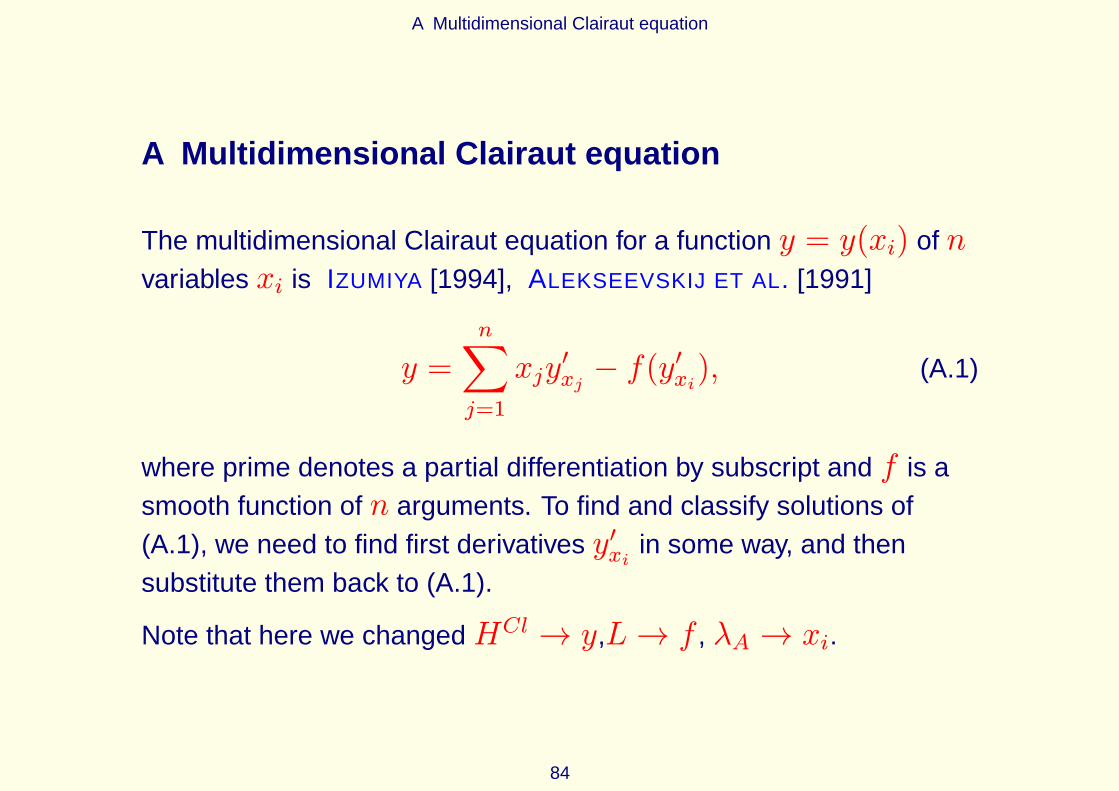
A Multidimensional Clairaut equation
The multidimensional Clairaut equation for a function y = y(xi) of nvariables xi is IZUMIYA [1994], ALEKSEEVSKIJ ET AL. [1991]
y =n∑
j=1
xjy′xj− f(y′xi), (A.1)
where prime denotes a partial differentiation by subscript and f is asmooth function of n arguments. To find and classify solutions of(A.1), we need to find first derivatives y′xi in some way, and thensubstitute them back to (A.1).
Note that here we changedHCl → y,L→ f , λA → xi.
84

A Multidimensional Clairaut equation
We differentiate the Clairaut equation (A.1) by xj and obtain nequations
n∑
i=1
y′′xixj(xi − f′y′xi) = 0. (A.2)
The classification follows from ways of vanishing the multipliers in(A.2). Here, for our physical applications, it is sufficient to supposethat ranks of Hessians of y and f are equal
rank y′′xixj = rank f′′y′xiy′xj= r. (A.3)
This means that in each equation from (A.2) whether first or secondmultiplier is zero, but it is not necessary to vanish both of them. Thefirst multiplier can be set to zero without any additional assumptions.
85

A Multidimensional Clairaut equation
So we have
1) The general solution. It is defined by the condition
y′′xixj = 0. (A.4)
After one integration we find y′xi = ci and substitution them to (A.1)and obtain
ygen =n∑
j=1
xjcj − f(ci), (A.5)
where ci are n constants.
All second multipliers in (A.2) can be zero for i = 1, . . . , n, but thiswill give a solution, if we can resolve them under y′xi . It can be
possible, if the rank of Hessians off is full, i.e. r = n. In this case weobtain
86
A Multidimensional Clairaut equation
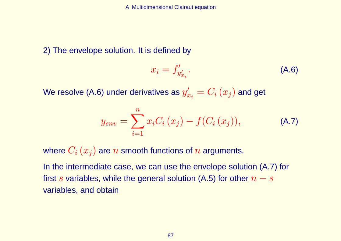
2) The envelope solution. It is defined by
xi = f′y′xi. (A.6)
We resolve (A.6) under derivatives as y′xi = Ci (xj) and get
yenv =n∑
i=1
xiCi (xj)− f(Ci (xj)), (A.7)
where Ci (xj) are n smooth functions of n arguments.
In the intermediate case, we can use the envelope solution (A.7) forfirst s variables, while the general solution (A.5) for other n− svariables, and obtain
87

A Multidimensional Clairaut equation
3) The s-mixed solution, as follows
y(s)mix =
s∑
j=1
xjCj (xj)+n∑
j=s+1
xjcj−f(C1 (xj) , . . . , Cs (xj) , cs+1, . . . , cn).
(A.8)
If the rank r of Hessians f is not full and a nonsingular minor of therank r is in upper left corner, then we can resolve first r relations (A.6)only, and so s ≤ r. In our physical applications we use the limitedcase s = r.
Example A.1. Let f (zi) = z21 + z
22 + z3, then the Clairaut equation
for y = y (x1, x2,x3) is
y = x1y′x1+ x2y
′x2+ x3y
′x3−(y′x1)2−(y′x2)2− y′x3 , (A.9)
and we have n = 3 and r = 2. The general solution can be found
88
A Multidimensional Clairaut equation
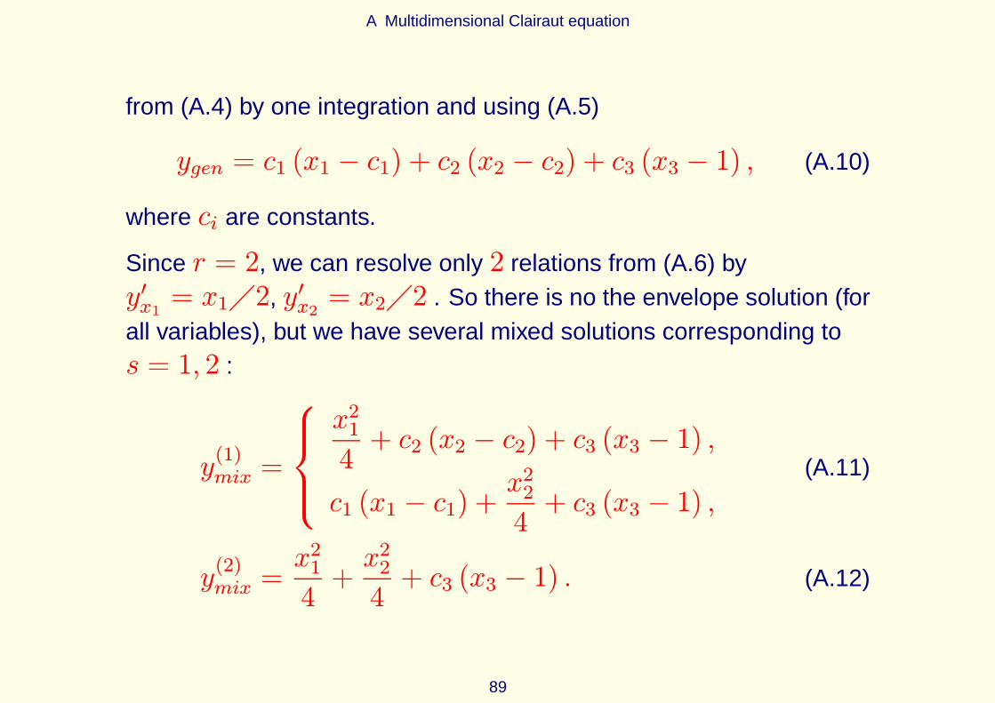
from (A.4) by one integration and using (A.5)
ygen = c1 (x1 − c1) + c2 (x2 − c2) + c3 (x3 − 1) , (A.10)
where ci are constants.
Since r = 2, we can resolve only 2 relations from (A.6) byy′x1 = x1�2, y
′x2= x2�2 . So there is no the envelope solution (for
all variables), but we have several mixed solutions corresponding tos = 1, 2 :
y(1)mix =
x214+ c2 (x2 − c2) + c3 (x3 − 1) ,
c1 (x1 − c1) +x224+ c3 (x3 − 1) ,
(A.11)
y(2)mix =
x214+x224+ c3 (x3 − 1) . (A.12)
89
A Multidimensional Clairaut equation
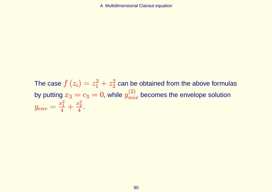
The case f (zi) = z21 + z
22 can be obtained from the above formulas
by putting x3 = c3 = 0, while y(2)mix becomes the envelope solution
yenv =x214+x224
.
90

B Examples
B Examples
Example B.1. Let L (x, v) = mv2/2− kx2/2, then the
corresponding Clairaut equation forH = HCl (x, λ) is
H = λH ′λ −m
2(H ′λ)
2+kx2
2, (B.1)
whereH ′λ denotes partial differentiation in λ. The general solution is
HClgen (x, λ, c) = λc−
mc2
2+kx2
2,
where c = c (x) is an arbitrary function (“unresolved velocity” v). Theenvelope solution (with λ = p) can be found from the condition
∂HCl
∂c= p−mc = 0 =⇒ cextr =
p
m,
91

B Examples
which gives
HClenv (x, p) =
p2
2m+kx2
2(B.2)
in the standard way.
Example B.2. Let L (x, v) = x exp v, then the corresponding
Clairaut equation forH = HCl (x, λ) is
H = λH ′λ − x exp (H′λ) . (B.3)
The general solution is
HClgen (x, λ) = λc (x)− x exp c (x) ,
The envelope solution (with λ = p) can be found from the condition
∂HCl
∂c= p− x exp c = 0 =⇒ cextr = ln
p
x,
92

B Examples
which leads to
HClenv (x, p) = p ln
p
x− p. (B.4)
Example B.3. Let L (x, y, vx, vy) = myv2x/2 + kxvy, then the
corresponding Clairaut equation forH = HCl (x, y, λx, λy) is
H = λxH′λx+ λyH
′λy−my
2
(H ′λx
)2− kxH ′λy , (B.5)
The general solution is
HClgen (x, y, λx, λy, cx, cy) = λxcx + λycy −
myc2x2− kxcy,
where cx, cy are arbitrary functions of the passive variables x, y.
93
B Examples
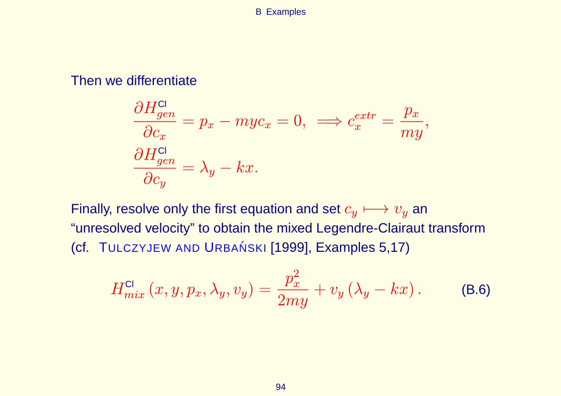
Then we differentiate
∂HClgen
∂cx= px −mycx = 0, =⇒ c
extrx =
px
my,
∂HClgen
∂cy= λy − kx.
Finally, resolve only the first equation and set cy 7−→ vy an“unresolved velocity” to obtain the mixed Legendre-Clairaut transform(cf. TULCZYJEW AND URBANSKI [1999], Examples 5,17)
HClmix (x, y, px, λy, vy) =
p2x2my
+ vy (λy − kx) . (B.6)
94

B Examples
Example B.4 (Cawley CAWLEY [1979]). Let L = xy + zy2/2, thenthe equations of motion are
x = yz, y = 0, y2 = 0. (B.7)
Because the Hessian has rank 2 and the velocity z does not enter intothe Lagrangian, the only degenerate velocity is z. The regularmomenta are px = y, py = x, and we have
Hphys = pxpy −1
2zy2, hy = 0.
The equations of motion (4.15)–(4.16) are
px = 0, py = yz, (B.8)
95

B Examples
and the condition (4.17) gives
DzHphys =∂Hphys
∂z= −1
2y2 = 0. (B.9)
Observe that (B.8) and (B.9) coincide with initial Lagrange equationsof motion (B.7).
Example B.5. Classical relativistic particle is described by
L = −mR, R =√x20 −
∑
i=x,y,z
x2i , (B.10)
where a dot denotes derivative with respect to the proper time.Because the rank of Hessian is 3, we consider velocities xi as regularvariables and the velocity x0 as degenerate variable. Then for theregular canonical momenta we have pi = mxi�R which can be
96

B Examples
resolved under the regular velocities as
xi = x0pi
E, E =
√m2 +
∑
i=x,y,z
p2i . (B.11)
Using (?? ) and (4.13) we obtain for Hamiltonians
Hphys = 0, hx0 = mx0
R= E, (B.12)
and so the “physical sense” of hx0 is, that it is indeed the energy(B.11). Equations of motion (4.15)–(4.16) are
xi = x0pi
E, pi = −
∂hx0∂xix0 = 0,
which coincide with the Lagrange equations following from (B.10)directly, the velocity x0 is arbitrary, and (4.17) becomes 0 = 0.
97

B Examples
Example B.6 (Christ-Lee model CHRIST AND LEE [1980]). TheLagrangian of SU (2) Yang-Mills theory in 0 + 1 dimensions is (inour notation)
L (xi, yα, vi) =1
2(vi − εijαxjyα)
2 − U(x2), (B.13)
where i, α = 1, 2, 3, x2 =∑i x2i , vi = xi and εijk is the
Levi-Civita symbol.
98

B Examples
The corresponding Clairaut equation (2.4) forH = HCl (xi, yα, λi, λα) has the form
H = λiH′λi+λαH
′λα−1
2
(H ′λi − εijαxjyα
)2+U
(x2). (B.14)
Its general solution is
Hgen = λici + λαcα −1
2(ci − εijαxjyα)
2 + U(x2), (B.15)
where ci, cα are functions of coordinates only (arbitrary constants).We differentiate (B.15) by them to get
∂Hgen
∂ci= λi − (ci − εijαxjyα) , (B.16)
∂Hgen
∂cα= λα, (B.17)
99

B Examples
and observe that only (B.16) can lead to the envelope solution. So we
can exclude the half of constants using (B.16) (with λi(6.15)→ pi) and
get the mixed solution (4.7) to the Clairaut equation (B.14) as
HClmix (xi, yα, pi, λα, cα) =1
2p2i + εijαpixjyα + λαcα + U
(x2).
(B.18)Using (4.12), we obtain the “physical” Hamiltonian
Hphys (xi, yα, pi) =1
2p2i + εijαpixjyα + U
(x2). (B.19)
From the other side, the Hessian of (B.13) has the rank 3, and wechoose xi, vi and yα to be regular and degenerate variablesrespectively.
100

B Examples
Because (B.13) independent of degenerate velocities yα, all
Bα(qA, pi
) (??)= 0, and therefore Fαβ
(qA, pi
) (7.8)= 0, we have the
limit gauge case of the above classification. So the degeneratevelocities vα = yα cannot be defined from (4.17) at all, they arearbitrary, and the first integrals (4.17), of the system (4.15)–(4.16)become (also in accordance to the independence statement)
∂Hphys (xi, yα, pi)
∂yα= εijαpixj = 0, (B.20)
and the preservation in time (B.20) is fulfilled identically due toproperties of the Levi-Civita symbols.
101

B Examples
It is clear, that only 2 equations from 3 ones of (B.20) are independent,we choose p1x2 = p2x1, p1x3 = p3x1 and insert in (B.19) to get
Hphys =1
2p21x2
x21+ U
(x2). (B.21)
The transformation p = p1√x2�x1, x =
√x2 gives the well-known
result CHRIST AND LEE [1980], GOGILIDZE ET AL. [1998]
Hphys =1
2p2 + U (x) . (B.22)
102

References
References
ABRAHAM, R. AND J. E. MARSDEN (1978). Foundations of Mechanics.Reading: Benjamin-Cummings.
ALART, P., O. MAISONNEUVE, AND R. T. ROCKAFELLAR (2006). NonsmoothMechanics and Analysis: Theoretical and Numerical Advances. Berlin:Springer-Verlag.
ALEKSEEVSKIJ, D. V., A. M. VINOGRADOV, AND V. V. LYCHAGIN (1991).Geometry I: Basic Ideas and Concepts of Differential Geometry. NewYork: Springer.
ARNOLD, V. I. (1988). Geometrical Methods in the Theory of OrdinaryDifferential Equations. New York: Springer-Verlag.
ARNOLD, V. I. (1989). Mathematical methods of classical mechanics. Berlin:Springer.
ARNOWITT, R., S. DESER, AND C. W. MISNER (1962). The dynamics ofGeneral Relativity. In: L. WITTEN (Ed.), Gravitation: An Introduction ToCurrent Research, New York: Wiley, pp. 227–264.
103

References
BARS, I. AND J. TERNING (2010). Why higher space or time dimensions? In:F. NEKOOGAR (Ed.), Extra Dimensions in Space and Time, Heidelberg:Springer, pp. 218.
BUEKEN, P. (1996). Multi-hamiltonian formulation for a class of degeneratecompletely integrable systems. J. Math. Phys. 37, 2851–2862.
CARINENA, J. F. (1990). Theory of singular Lagrangians. Fortsch. Physik 38(9), 641–679.
CAWLEY, R. (1979). Determination of the Hamiltonian in the presence ofconstraints. Phys. Rev. Lett. 42 (7), 413–416.
CENDRA, H., D. D. HOLM, M. J. V. HOYLE, AND J. E. MARSDEN (1998).The Maxwell-Vlasov equations in Euler-Poincare form. J. Math. Phys. 39(6), 3138–3157.
CHRIST, N. H. AND T. D. LEE (1980). Operator ordering and feynman rulesin gauge theories. Phys. Rev. D22 (4), 939–958.
CLARKE, F. H. (1977). Extremal arcs and extended Hamiltonian systems.Trans. Amer. Math. Soc. 231 (2), 349–367.
104

References
DELIGNE, P., P. ETINGOF, D. S. FREED, L. C. JEFFREY, D. KAZHDAN, J. W.MORGAN, D. R. MORRISON, AND E. WITTEN (Eds.) (1999). QuantumFields and Strings: A Cource for Mathematicians, Volume 1, 2,Providence. American Mathematical Society.
DIRAC, P. A. M. (1964). Lectures on Quantum Mechanics. New York:Yeshiva University.
DORLING, J. (1970). The dimensionality of time. Am. J. Phys. 38, 539–540.
DUPLIJ, S. (2009a). Analysis of constraint systems using the Clairautequation. In: B. DRAGOVICH AND Z. RAKIC (Eds.), Proceedings of 5thMathematical Physics Meeting: Summer School in Modern MathematicalPhysics, 6 - 17 July 2008, Belgrade: Institute of Physics, pp. 217–225.
DUPLIJ, S. (2009b). Generalized duality, Hamiltonian formalism and newbrackets, preprint Kharkov National University, Kharkov, 24 p.,arXiv:math-ph/1002.1565v7 (To appear in J. Math. Phys. Analysis. Geom.,2013).
105
References
DUPLIJ, S. (2011). A new Hamiltonian formalism for singular Lagrangiantheories. J. Kharkov National Univ., ser. Nuclei, Particles and Fields 969(3(51)), 34–39.
DUPLIJ, S. (2013). Partial Hamiltonian formalism, multi-time dynamics andsingular theories. J. Kharkov National Univ., ser. Nuclei, Particles andFields 1059 (3(59)), 10–21.
DUPLIJ, S. (2014). Generalized duality, Hamiltonian formalism and newbrackets. J. Math. Physics, Analysis, Geometry 10 (2), 189–220.
DUPLIJ, S. (2015). Formulation of singular theories in a partial Hamiltonianformalism using a new bracket and multi-time dynamics. Int. J. Geom.Meth. Mod. Phys. 12 (01), 1550001.
DVALI, G., G. GABADADZE, AND G. SENJANOVIC (2000). Constraints onextra time dimensions. In: M. A. SHIFMAN (Ed.), The Many Faces of theSuperworld: Yuri Golfand Memorial Volume, Singapore: World Scientific.
FAIRLIE, D. B., P. FLETCHER, AND C. K. ZACHOS (1990).Infinite-dimensional algebras and a trigonometric basis for the classicalLie algebras. J. Math. Phys. 31 (5), 1088–1094.
106

References
FENCHEL, W. (1949). On conjugate convex functions. Canad. J. Math. 1,73–77.
FLORATOS, E. G., J. ILIOPOULOS, AND G. TIKTOPOULOS (1989). A note onSU(∞) classical Yang-Mills theories. Phys. Lett. 217 (3), 285–288.
GITMAN, D. M. AND I. V. TYUTIN (1986). Canonical quantization ofconstrained fields. M.: Nauka.
GITMAN, D. M. AND I. V. TYUTIN (1990). Quantization of Fields withConstraints. Berlin: Springer-Verlag.
GOGILIDZE, S. A., A. M. KHVEDELIDZE, D. M. MLADENOV, AND H.-P. PAVEL
(1998). Hamiltonian reduction of SU(2) Dirac-Yang-Mills mechanics.Phys. Rev. D57 (12), 7488–7500.
GOGILIDZE, S. A., A. M. KHVEDELIDZE, AND V. N. PERVUSHIN (1996). OnAbelianization of first class constraints. J. Math. Phys. 37 (4), 1760–1771.
GOLDSTEIN, H. (1990). Classical Mechanics. Reading: Addison-Wesley.
107

References
IOFFE, A. (1997). Euler-Lagrange and Hamiltonian formalisms in dynamicoptimization. Trans. Amer. Math. Soc. 349, 2871–2900.
IZUMIYA, S. (1994). Systems of Clairaut type. Colloq. Math. 66 (2), 219–226.
KAMKE, E. (1928). Ueber Clairautsche Differentialgleichung. Math. Zeit. 27(1), 623–639.
LANCZOS, C. (1962). The variational principles of mechanics (Second ed.).Toronto: Univ. Toronto Press.
LANDAU, L. D. AND E. M. LIFSHITZ (1969). Mechanics. Oxford: PergamonPress.
LONGHI, G., L. LUSANNA, AND J. M. PONS (1989). On the many-timeformulation of classical particle dynamics. J. Math. Phys. 30 (8),1893–1912.
LORAN, F. (2005). Non-Abelianizable first class constraints. Commun. Math.Phys. 254, 167–178.
108
References
MARMO, G., E. J. SALETAN, A. SIMONI, AND B. VITALE (1985). DynamicalSystems: a Differential Geometric Approach to Symmetry and Reduction.Chichester: J. Wiley.
PONS, J. M. (2005). On Dirac’s incomplete analysis of gaugetransformations. Stud. Hist. Philos. Mod. Phys. 36, 491–518.
REGGE, T. AND C. TEITELBOIM (1976). Constrained Hamiltonian Systems.Rome: Academia Nazionale dei Lincei.
ROCKAFELLAR, R. T. (1967). Conjugates and Legendre transforms ofconvex functions. Canad. J. Math. 19, 200–205.
ROCKAFELLAR, R. T. (1970). Convex Analysis. Princeton: PrincetonUniversity Press.
SAVELIEV, M. V. AND A. M. VERSHIK (1990). New examples of continuumgraded Lie algebras. Phys. Lett. A143, 121–128.
STERNBERG, S. (1954). Legendre transformation of curves. Proc. Amer.Math. Soc. 5 (6), 942–945.
109

References
SUDARSHAN, E. C. AND N. MUKUNDA (1974). Classical Dynamics: AModern Perspective. New York: Wiley.
SUNDERMEYER, K. (1982). Constrained Dynamics. Berlin: Springer-Verlag.
TULCZYJEW, W. M. (1977). The Legendre transformation. Ann. Inst. HenriPoincare A27 (1), 101–114.
TULCZYJEW, W. M. (1989). Geometric formulation of physical theories.Naples: Bibliopolis.
TULCZYJEW, W. M. AND P. URBANSKI (1999). A slow and careful Legendretransformation for singular Lagrangians. Acta Phys. Pol. B30 (10),2909–2977.
VALLEE, C., M. HJIAJ, D.FORTUNE, AND G. DE SAXCE (2004). GeneralizedLegendre-Fenchel transformation. Adv. Mech. Math. 6, 289–312.
WALKER, M. L. AND S. DUPLIJ (2015). Cho-Duan-Ge decomposition of QCDin the constraintless Clairaut-type formalism. Phys.Rev. D91 (6), 064022.
110

References
WEINBERG, S. (1995–2000). The Quantum Theory of Fields. Vols. 1,2,3.Cambridge: Cambridge University Press.
ZACHOS, C. (1990). Hamiltonian flows, SU(∞), SO(∞), USp(∞), andstrings. In: L.-L. CHAU AND W. NAHM (Eds.), Differential GeometricMethods in Theoretical Physics: Physics and Geometry, NATO ASI, NewYork: Plenum Press, pp. 423–430.
111