s2.bitdownload.irs2.bitdownload.ir/ebook/calculus/bounded analytic functions - j... ·...
TRANSCRIPT
Graduate Texts in Mathematics 236
Editorial BoardS. Axler K.A. Ribet

1 TAKEUTI/ZARING. Introduction toAxiomatic Set Theory. 2nd ed.
2 OXTOBY. Measure and Category. 2nd ed.3 SCHAEFER. Topological Vector Spaces.
2nd ed.4 HILTON/STAMMBACH. A Course in
Homological Algebra. 2nd ed.5 MAC LANE. Categories for the Working
Mathematician. 2nd ed.6 HUGHES/PIPER. Projective Planes.7 J.-P. SERRE. A Course in Arithmetic.8 TAKEUTI/ZARING. Axiomatic Set Theory.9 HUMPHREYS. Introduction to Lie
Algebras and Representation Theory.10 COHEN. A Course in Simple Homotopy
Theory.11 CONWAY. Functions of One Complex
Variable I. 2nd ed.12 BEALS. Advanced Mathematical Analysis.13 ANDERSON/FULLER. Rings and
Categories of Modules. 2nd ed.14 GOLUBITSKY/GUILLEMIN. Stable
Mappings and Their Singularities.15 BERBERIAN. Lectures in Functional
Analysis and Operator Theory.16 WINTER. The Structure of Fields.17 ROSENBLATT. Random Processes. 2nd ed.18 HALMOS. Measure Theory.19 HALMOS. A Hilbert Space Problem
Book. 2nd ed.20 HUSEMOLLER. Fibre Bundles. 3rd ed.21 HUMPHREYS. Linear Algebraic Groups.22 BARNES/MACK. An Algebraic
Introduction to Mathematical Logic.23 GREUB. Linear Algebra. 4th ed.24 HOLMES. Geometric Functional
Analysis and Its Applications.25 HEWITT/STROMBERG. Real and Abstract
Analysis.26 MANES. Algebraic Theories.27 KELLEY. General Topology.28 ZARISKI/SAMUEL. Commutative
Algebra. Vol. I.29 ZARISKI/SAMUEL. Commutative
Algebra. Vol. II.30 JACOBSON. Lectures in Abstract Algebra
I. Basic Concepts.31 JACOBSON. Lectures in Abstract Algebra
II. Linear Algebra.32 JACOBSON. Lectures in Abstract Algebra
III. Theory of Fields and GaloisTheory.
33 HIRSCH. Differential Topology.
34 SPITZER. Principles of Random Walk.2nd ed.
35 ALEXANDER/WERMER. Several ComplexVariables and Banach Algebras. 3rd ed.
36 KELLEY/NAMIOKA et al. LinearTopological Spaces.
37 MONK. Mathematical Logic.38 GRAUERT/FRITZSCHE. Several Complex
Variables.39 ARVESON. An Invitation to C*-Algebras.40 KEMENY/SNELL/KNAPP. Denumerable
Markov Chains. 2nd ed.41 APOSTOL. Modular Functions and
Dirichlet Series in Number Theory.2nd ed.
42 J.-P. SERRE. Linear Representations ofFinite Groups.
43 GILLMAN/JERISON. Rings ofContinuous Functions.
44 KENDIG. Elementary AlgebraicGeometry.
45 LOÈVE. Probability Theory I. 4th ed.46 LOÈVE. Probability Theory II. 4th ed.47 MOISE. Geometric Topology in
Dimensions 2 and 3.48 SACHS/WU. General Relativity for
Mathematicians.49 GRUENBERG/WEIR. Linear Geometry.
2nd ed.50 EDWARDS. Fermat's Last Theorem.51 KLINGENBERG. A Course in Differential
Geometry.52 HARTSHORNE. Algebraic Geometry.53 MANIN. A Course in Mathematical Logic.54 GRAVER/WATKINS. Combinatorics with
Emphasis on the Theory of Graphs.55 BROWN/PEARCY. Introduction to
Operator Theory I: Elements ofFunctional Analysis.
56 MASSEY. Algebraic Topology: AnIntroduction.
57 CROWELL/FOX. Introduction to KnotTheory.
58 KOBLITZ. p-adic Numbers, p-adicAnalysis, and Zeta-Functions. 2nd ed.
59 LANG. Cyclotomic Fields.60 ARNOLD. Mathematical Methods in
Classical Mechanics. 2nd ed.61 WHITEHEAD. Elements of Homotopy
Theory.62 KARGAPOLOV/MERIZJAKOV.
Fundamentals of the Theory of Groups.63 BOLLOBAS. Graph Theory.
Graduate Texts in Mathematics
(continued after index)
John B. Garnett
Bounded AnalyticFunctions
Revised First Edition

John B. GarnettDepartment of Mathematics6363 Mathematical SciencesUniversity of California, Los AngelesLos Angeles, CA. 90095–[email protected]
Editorial Board:S. Axler K.A. RibetDepartment of Mathematics Depratment of MathematicsSan Francisco State University University of California, BerkeleySan Francisco, CA 94132 Berkeley, CA 94720-3840USA [email protected] [email protected]
Previously published by Academic Press, Inc.San Diego, CA 92101
Mathematics: Subject Classification (2000): 30D55 30–02 46315
Library of Congress Control Number: 2006926458
ISBN-13: 978-0387-33621-3ISBN-10: 0-387-33621-4
Printed on acid-free paper.
© 2007 Springer Science+Business Media, LLCAll rights reserved. This work may not be translated or copied in whole or in part without the writtenpermission of the publisher (Springer Science+Business Media, LLC, 233 Spring Street, New York,NY 10013, USA), except for brief excerpts in connection with reviews or scholarly analysis. Usein connection with any form of information storage and retrieval, electronic adaptation, computersoftware, or by similar or dissimilar methodology now known or hereafter developed is forbidden.The use in this publication of trade names, trademarks, service marks, and similar terms, even if theyare not identified as such, is not to be taken as an expression of opinion as to whether or not they aresubject to proprietary rights.
9 8 7 6 5 4 3 2 1
springer.com

To Dolores

Preface to Revised First Edition
This edition of Bounded Analytic Functions is the same as the first edition exceptfor the corrections of several mathematical and typographical errors. I thank themany colleagues and students who have pointed out errors in the first edition.These include S. Axler, C. Bishop, A. Carbery, K. Dyakonov, J. Handy, V. Havin, H.Hunziker, P. Koosis, D. Lubinsky, D. Marshall, R. Mortini, A. Nicolau, M. O’Neill,W. Rudin, D. Sarason, D. Suarez, C. Sundberg, C. Thiele, S. Treil, I. Uriarte-Tuero,J. Vaisala, N. Varopoulos, and L. Ward.
I had planned to prepare a second edition with an updated bibliography and anappendix on results new in the field since 1981, but that work has been postponed fortoo long. In the meantime several excellent related books have appeared, includingM. Andersson, Topics in Complex Analysis; G. David and S. Semmes, SingularIntegrals and Rectifiable Sets in �n and Analysis of and on Uniformly Rectifi-able Sets; S. Fischer, Function theory on planar domains; P. Koosis, Introductionto Hp spaces, Second edition; N. Nikolski, Operators, Functions, and Systems;K. Seip, Interpolation and Sampling in Spaces of Analytic Functions; and B. Simon,Orthogonal Polynomials on the Unit Circle.
Several problems posed in the first edition have been solved. I give referencesonly to Mathematical Reviews. The question page 167 on when E∞ contains aBlaschke product was settled by A. Stray in MR 0940287. M. Papadimitrakis, MR0947674, gave a counterexample to the conjecture in Problem 5 page 170. The lateT. Wolff, MR 1979771, had a counterexample to the Baernstein conjecture citedon page 260. S. Treil resolved the g2 problem on page 319 in MR 1945294. Aconstructive Fefferman-Stein decomposition of functions in BMO(�n) was givenby the late A. Uchiyama in MR 1007515, and C. Sundberg, MR 0660188, founda constructive proof of the Chang-Marshall theorem. Problem 5.3 page 420 wasresolved by Garnett and Nicolau, MR 1394402, using work of Marshall and StrayMR 1394401. Problem 5.4. on page 420 remains a puzzle, but Hjelle and Nicolau(Pacific Journal of Mathematics, 2006) have an interesting result on approximationof moduli. P. Jones, MR 0697611, gave a construction of the P. Beurling linearoperator of interpolation.
I thank Springer and F. W. Gehring for publishing this edition.
John Garnett
vii

Contents
Preface viiList of Symbols xiii
I. PRELIMINARIES
1. Schwarz’s Lemma 12. Pick’s Theorem 53. Poisson Integrals 104. Hardy–Littlewood Maximal Function 195. Nontangential Maximal Function and Fatou’s Theorem 276. Subharmonic Functions 32
Notes 38Exercises and Further Results 39
II. H P SPACES
1. Definitions 482. Blaschke Products 513. Maximal Functions and Boundary Values 554. (1/π )
∫(log | f (t)|/(1 + t2))dt >− ∞ 61
5. The Nevanlinna Class 666. Inner Functions 717. Beurling’s Theorem 78
Notes 83Exercises and Further Results 84
III. CONJUGATE FUNCTIONS
1. Preliminaries 982. The L p Theorems 1063. Conjugate Functions and Maximal Functions 111
ix
x contents
Notes 118Exercises and Further Results 120
IV. SOME EXTREMAL PROBLEMS
1. Dual Extremal Problems 1282. The Carleson–Jacobs Theorem 1343. The Helson–Szego Theorem 1394. Interpolating Functions of Constant Modulus 1455. Parametrization of K 1516. Nevanlinna’s Proof 159
Notes 168Exercises and Further Results 168
V. SOME UNIFORM ALGEBRA
1. Maximal Ideal Spaces 1762. Inner Functions 1863. Analytic Discs in Fibers 1914. Representing Measures and Orthogonal Measures 1935. The Space L1/H 1
0 198Notes 205Exercises and Further Results 206
VI. BOUNDED MEAN OSCILLATION
1. Preliminaries 2152. The John–Nirenberg Theorem 2233. Littlewood–Paley Integrals and Carleson Measures 2284. Fefferman’s Duality Theorem 2345. Vanishing Mean Oscillation 2426. Weighted Norm Inequalities 245
Notes 259Exercises and Further Results 261
VII. INTERPOLATING SEQUENCES
1. Carleson’s Interpolation Theorem 2752. The Linear Operator of Interpolation 2853. Generations 2894. Harmonic Interpolation 2925. Earl’s Elementary Proof 299
Notes 304Exercises and Further Results 305

contents xi
VIII. THE CORONA CONSTRUCTION
1. Inhomogeneous Cauchy–Riemann Equations 3092. The Corona Theorem 3143. Two Theorems on Minimum Modulus 3234. Interpolating Blaschke Products 3275. Carleson’s Construction 3336. Gradients of Bounded Harmonic Functions 3387. A Constructive Solution of ∂b/∂z = μ 349
Notes 357Exercises and Further Results 358
IX. DOUGLAS ALGEBRAS
1. The Douglas Problem 3642. H∞ + C 3673. The Chang-Marshall Theorem 3694. The Structure of Douglas Algebras 3755. The Local Fatou Theorem and an Application 379
Notes 384Exercises and Further Results 385
X. INTERPOLATING SEQUENCES AND MAXIMAL IDEALS
1. Analytic Discs in M 3912. Hoffman’s Theorem 4013. Approximate Dependence between Kernels 4064. Interpolating Sequences and Harmonic Separation 4125. A Constructive Douglas–Rudin Theorem 418
Notes 428Exercises and Further Results 428
BIBLIOGRAPHY 434
INDEX 453

List of Symbols
Symbol Page
Ao 120Am 121A∞ 121Aα 57A−1 176
A 179A⊥ 196AN 57B 237B0 274BLO 271BMO 216BMOA 262BMO(T ) 218BMOd 266BUC 242[B, H ] 270B = { f analytic,| f (z)| ≤ 1} 7B , a set of inner functions 364B A 364C = C(T ) 128COP 432CA 367Cl( f, z) 76D 1D 1dist( f, H p) 129dist∗ 241D 391∂/∂z 312∂/∂z 309∂ 354E∗ 323
Symbol Page
|E | = Lebesgue measure of E 23E 292f (m) 180
f (m) = Gelfand transform 178
f (s) = Fourier transform 59fx (t) 15f +(x) 324f #(x) 271f ∗(t) 55( f )∗(θ ) 106G 401Gδ(b) 371Hf (θ ) 102Hf (x) 105Hε f (x) 123H∗ f (x) 123H p = H p(D) 48H p = H p(dt) 49H∞ 48Hq
0 128H 1
d 267H 1
R236
(H∞)−1 63H∞ + C 132[H∞, B ] 364[H∞,U A] 365H 5I 221Jm 404J ( f1, f2, . . . , fn) 319K (z0, r ) 2Kδ(B) 401LC(x) 235
xiii
xiv list of symbols
Symbol Page
L1loc
215Lp
R236
L∞R
64Lz(ζ ) 392log +| f (z)| 33(Q) 278L 394m( f ) = f (m) = f (m) 180m(λ) 20M(T ) 128M f (x) 21M(dμ)(t) 28Mδ(ϕ) 242Mμ f (x) 45M 183MA 178Mζ 183MD 394N 66N (σ ) 30N+ 68Nε(x) 339norms: ‖ f ‖p
H p 48, 49‖ϕ‖∗ 216‖ϕ‖′ 250‖u‖H1
236Pz0
(θ ) 10Pz0
(t) 11P(m) 393Qr (ϕ) 99Qz(ϕ) 98QC 367Q A 366� = real numbers 12R ( f, z0) 77S(θ0, h) 371S j 334S h 153T 98
Symbol Page
T (Q) 290u+(t) 116u∗(t) 27u(z) 98UC 242U A 365vr (z) 35VMO 242VMOA 274VMOA 375X 181Xζ 207β� 180δ(B) 327�(c, R) 3�u 10ε(ρ) 250, 258�α(t) 21�α(eiθ ) 23�h
α(t) 379λϕ 233λ∗ 433�α 102�∗ 273μϕ 233ν f 371ρ(z, w) 2ρ(m1, m2) 392ρ(S, T ) 305ϕI 216ω(δ) 101ω f (δ) 101∇g 228
|∇g |2 228∗ 13z = complex conjugate of zf = complex conjugate of fF = { f : f ∈ F}, when F is a set of
functionsE = closure of E , when E is a point set

I
Preliminaries
As a preparation, we discuss three topics from elementary real or complexanalysis which will be used throughout this book.
The first topic is the invariant form of Schwarz’s lemma. It gives rise tothe pseudohyperbolic metric, which is an appropriate metric for the study ofbounded analytic functions. To illustrate the power of the Schwarz lemma, weprove Pick’s theorem on the finite interpolation problem
f (z j ) = w j , j = 1, 2, . . . , n,
with | f (z)| ≤ 1.The second topic is from real analysis. It is the circle of ideas relating Poisson
integrals to maximal functions.The chapter ends with a brief introduction to subharmonic functions and
harmonic majorants, our third topic.
1. Schwarz’s Lemma
Let D be the unit disc {z : |z| < 1} in the complex plane and let B denotethe set of analytic functions from D into D. Thus | f (z)| ≤ 1 if f ∈ B . Thesimple but surprisingly powerful Schwarz lemma is this:
Lemma 1.1. If f (z) ∈ B , and if f (0) = 0, then
| f (z)| ≤ |z|, z �= 0,
| f ′(0)| ≤ 1 .(1.1)
Equality holds in (1.1) at some point z if and only if f (z) = eiϕz, ϕ a realconstant.
The proof consists in observing that the analytic function g(z) = f (z)/zsatisfies |g| ≤ 1 by virtue of the maximum principle.
We shall use the invariant form of Schwarz’s lemma due to Pick. AMobius transformation is a conformal self-map of the unit disc. Every Mobius
1

2 preliminaries Chap. I
transformation can be written as
τ (z) = eiϕ z − z0
1 − z0z
with ϕ real and |z0| ≤ 1. With this notation we have displayed z0 = τ−1(0).
Lemma 1.2. If f (z) ∈ B , then
| f (z) − f (z0)||1 − f (z0) f (z)| ≤
∣∣∣∣
z − z0
1 − z0z
∣∣∣∣ , z �= z0,(1.2)
and
| f ′(z)|1 − | f (z)|2 ≤ 1
1 − |z|2 .(1.3)
Equality holds at some point z if and only if f (z) is a Mobius transformation.
The proof is the same as the proof of Schwarz’s lemma if we regard τ (z) asthe independent variable and
f (z) − f (z0)
1 − f (z0) f (z)
as the analytic function. Letting z tend to z0 in (1.2) gives (1.3) at z = z0, anarbitrary point of D.
The pseudohyperbolic distance on D is defined by
ρ(z, w) =∣∣∣∣
z − w
1 − wz
∣∣∣∣ .
Lemma 1.2 says that analytic mappings from D to D are Lipschitz continuousin the pseudohyperbolic distance:
ρ( f (z), f (w)) ≤ ρ(z, w).
The lemma also says that the distance ρ(z, w) is invariant under Mobiustransformations:
ρ(z, w) = ρ(τ (z), τ (w)).
We write K (z0, r ) for the noneuclidean disc
K (z0, r ) = {z : ρ(z, z0) < r}, 0 < r < 1.
Since the family B is invariant under the Mobius transformations, the study ofthe restrictions to K (z0, r ) of functions in B is the same as the study of theirrestrictions to K (0, r ) = {|w| < r}. In such a study, however, we must giveK (z0, r ) the coordinate function w = τ (z) = (z − z0)/(1 − z0z). For example,the set of derivatives of functions in B do not form a conformally invariant
Sect. 1 schwarz’s lemma 3
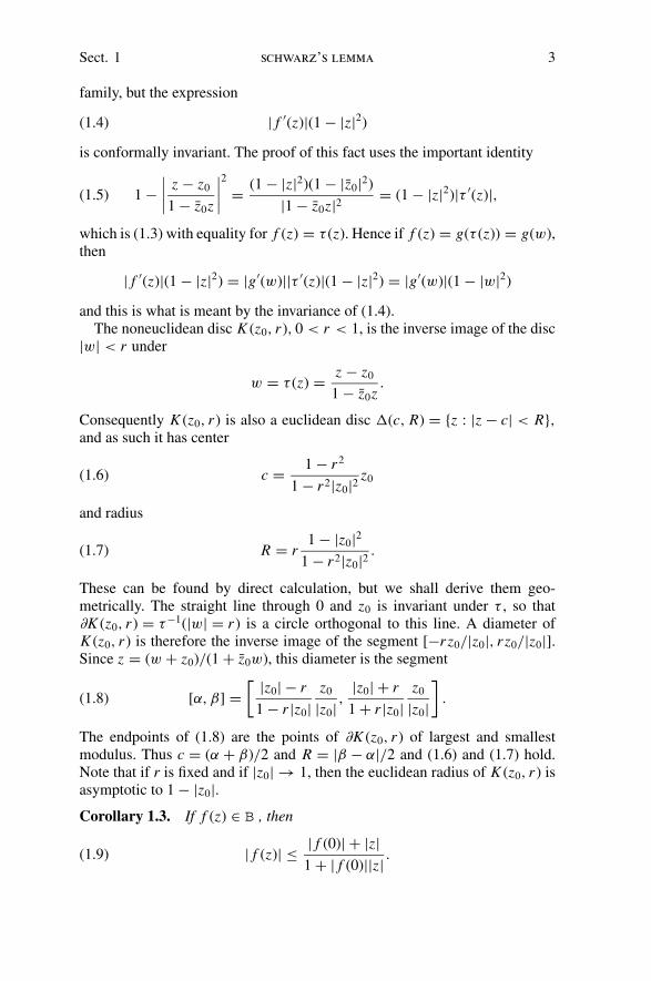
family, but the expression
| f ′(z)|(1 − |z|2)(1.4)
is conformally invariant. The proof of this fact uses the important identity
1 −∣∣∣∣
z − z0
1 − z0z
∣∣∣∣
2
= (1 − |z|2)(1 − |z0|2)
|1 − z0z|2 = (1 − |z|2)|τ ′(z)|,(1.5)
which is (1.3) with equality for f (z) = τ (z). Hence if f (z) = g(τ (z)) = g(w),then
| f ′(z)|(1 − |z|2) = |g′(w)||τ ′(z)|(1 − |z|2) = |g′(w)|(1 − |w|2)
and this is what is meant by the invariance of (1.4).The noneuclidean disc K (z0, r ), 0 < r < 1, is the inverse image of the disc
|w| < r under
w = τ (z) = z − z0
1 − z0z.
Consequently K (z0, r ) is also a euclidean disc �(c, R) = {z : |z − c| < R},and as such it has center
c = 1 − r2
1 − r2|z0|2 z0(1.6)
and radius
R = r1 − |z0|2
1 − r2|z0|2 .(1.7)
These can be found by direct calculation, but we shall derive them geo-metrically. The straight line through 0 and z0 is invariant under τ , so that∂K (z0, r ) = τ−1(|w| = r ) is a circle orthogonal to this line. A diameter ofK (z0, r ) is therefore the inverse image of the segment [−r z0/|z0|, r z0/|z0|].Since z = (w + z0)/(1 + z0w), this diameter is the segment
[α, β] =[ |z0| − r
1 − r |z0|z0
|z0| ,|z0| + r
1 + r |z0|z0
|z0|]
.(1.8)
The endpoints of (1.8) are the points of ∂K (z0, r ) of largest and smallestmodulus. Thus c = (α + β)/2 and R = |β − α|/2 and (1.6) and (1.7) hold.Note that if r is fixed and if |z0| → 1, then the euclidean radius of K (z0, r ) isasymptotic to 1 − |z0|.Corollary 1.3. If f (z) ∈ B , then
| f (z)| ≤ | f (0)| + |z|1 + | f (0)||z| .(1.9)
4 preliminaries Chap. I
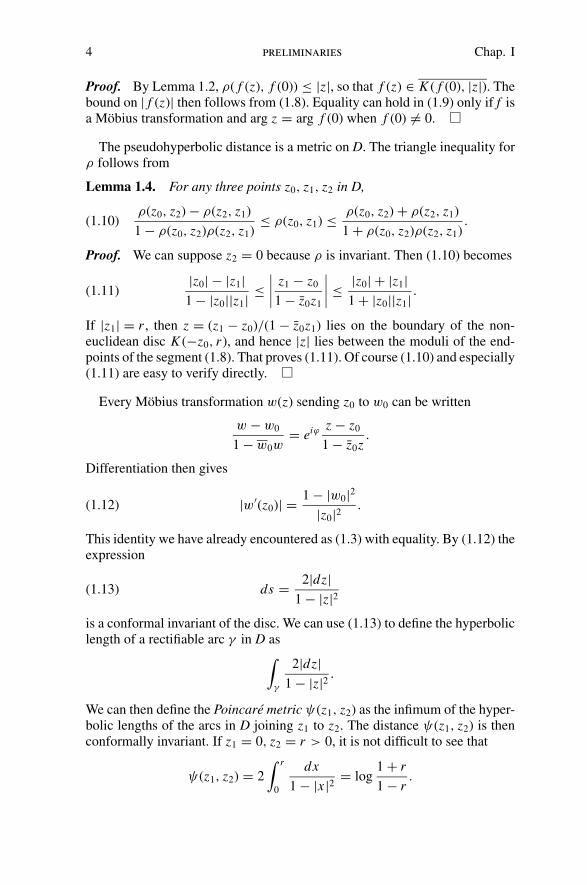
Proof. By Lemma 1.2, ρ( f (z), f (0)) ≤ |z|, so that f (z) ∈ K ( f (0), |z|). Thebound on | f (z)| then follows from (1.8). Equality can hold in (1.9) only if f isa Mobius transformation and arg z = arg f (0) when f (0) �= 0.
The pseudohyperbolic distance is a metric on D. The triangle inequality forρ follows from
Lemma 1.4. For any three points z0, z1, z2 in D,
ρ(z0, z2) − ρ(z2, z1)
1 − ρ(z0, z2)ρ(z2, z1)≤ ρ(z0, z1) ≤ ρ(z0, z2) + ρ(z2, z1)
1 + ρ(z0, z2)ρ(z2, z1).(1.10)
Proof. We can suppose z2 = 0 because ρ is invariant. Then (1.10) becomes
|z0| − |z1|1 − |z0||z1| ≤
∣∣∣∣
z1 − z0
1 − z0z1
∣∣∣∣ ≤ |z0| + |z1|
1 + |z0||z1| .(1.11)
If |z1| = r , then z = (z1 − z0)/(1 − z0z1) lies on the boundary of the non-euclidean disc K (−z0, r ), and hence |z| lies between the moduli of the end-points of the segment (1.8). That proves (1.11). Of course (1.10) and especially(1.11) are easy to verify directly.
Every Mobius transformation w(z) sending z0 to w0 can be written
w − w0
1 − w0w= eiϕ z − z0
1 − z0z.
Differentiation then gives
|w′(z0)| = 1 − |w0|2|z0|2 .(1.12)
This identity we have already encountered as (1.3) with equality. By (1.12) theexpression
ds = 2|dz|1 − |z|2(1.13)
is a conformal invariant of the disc. We can use (1.13) to define the hyperboliclength of a rectifiable arc γ in D as
∫
γ
2|dz|1 − |z|2 .
We can then define the Poincare metric ψ(z1, z2) as the infimum of the hyper-bolic lengths of the arcs in D joining z1 to z2. The distance ψ(z1, z2) is thenconformally invariant. If z1 = 0, z2 = r > 0, it is not difficult to see that
ψ(z1, z2) = 2
∫ r
0
dx
1 − |x |2 = log1 + r
1 − r.

Sect. 2 pick’s theorem 5
Since any pair of points z1 and z2 can be mapped to 0 and ρ(z1, z2) =|(z2 − z1)/(1 − z1z2)|, respectively, by a Mobius transformation, we thereforehave
ψ(z1, z2) = log1 + ρ(z1, z2)
1 − ρ(z1, z2).
A calculation then gives
ρ(z1, z2) = tanh
(ψ(z1, z2)
2
)
Moreover, because the shortest path from 0 to r is the radius, the geodesics, orpaths of shortest distance, in the Poincare metric consist of the images of thediameter under all Mobius transformations. These are the diameters of D andthe circular arcs in D orthogonal to ∂D. If these arcs are called lines, we havea model of the hyperbolic geometry of Lobachevsky.
In this book we shall work with the pseudohyperbolic metric ρ rather thanwith ψ , although the geodesics are often lurking in our intuition.
Hyperbolic geometry is somewhat simpler in the upper half plane H ={z = x + iy : y > 0} In H
ρ(z1, z2) =∣∣∣∣z1 − z2
z1 − z2
∣∣∣∣
and the element of hyperbolic arc length is
ds = |dz|y
.
Geodesics are vertical lines and circles orthogonal to the real axis. The con-formal self-maps of H that fix the point at ∞ have a very simple form:
τ (z) = az + x0, a > 0, x0 ∈ �.
Horizontal lines {y = y0} can be mapped to one another by these self-maps ofH . This is not the case in D with the circles {|z| = r}. In H any two squares
{x0 < x < x0 + h, h < y < 2h}are congruent in the noneuclidean geometry. The corresponding congruentfigures in D are more complicated. For these and for other reasons, H is oftenthe more convenient domain for many problems.
2. Pick’s Theorem
A finite Blaschke product is a function of the form
B(z) = eiϕn∏
j=1
z − z j
1 − z j z, |z j | < 1.

6 preliminaries Chap. I
The function B has the properties
(i) B is continuous across ∂D,(ii) |B| = 1 on ∂D, and
(iii) B has finitely many zeros in D.
These properties determine B up to a constant factor of modulus one. Indeed,if an analytic function f (z) has (i)–(iii), and if B(z) is a finite Blaschke productwith the same zeros, then by the maximum principle, | f/B| ≤ 1 and |B/ f | ≤ 1,on D, and so f/B is constant. The degree of B is its number of zeros. A Blaschkeproduct of degree 0 is a constant function of absolute value 1.
Theorem 2.1 (Caratheodory). If f (z) ∈ B , then there is a sequence {Bk} offinite Blaschke products that converges to f (z) pointwise on D.
Proof. Write
f (z) = c0 + c1z + · · · .
By induction, we shall find a Blaschke product of degree at most n whose firstn coefficients match those of f ;
Bn = c0 + c1z + · · · + cn−1zn−1 + dnzn + · · · .
That will prove the theorem. Since |c0| ≤ 1, we can take
B0 = z + c0
1 + c0z.
If |c0| = 1, then B0 = c0 is a Blaschke product of degree 0. Suppose that foreach g ∈ B we have constructed Bn−1(z). Set
g = 1
z
f − f (0)
1 − f (0) f
and let Bn−1 be a Blaschke product of degree at most n − 1 such that g − Bn−1
has n − 1 zeros at 0. Then zg − zBn−1 has n zeros at z = 0. Set
Bn(z) = zBn−1(z) + f (0)
1 + f (0)zBn−1(z).
Then Bn is a finite Blaschke product, degree(Bn) = degree(zBn−1) ≤ n, and
f (z) − Bn(z) = zg(z) + f (0)
1 + f (0)zg(z)− zBn−1(z) + f (0)
1 + f (0)zBn−1(z)
= (1 − | f (0)|2)z(g(z) − Bn−1(z))
(1 + f (0)zg(z))(1 + f (0)zBn−1(z)),
so that f − Bn has a zero of order n at z = 0.
The coefficient sequences {c0, c1, . . . .} of functions inB were characterizedby Schur [1917]. Instead of giving Schur’s theorem, we shall prove Pick’s
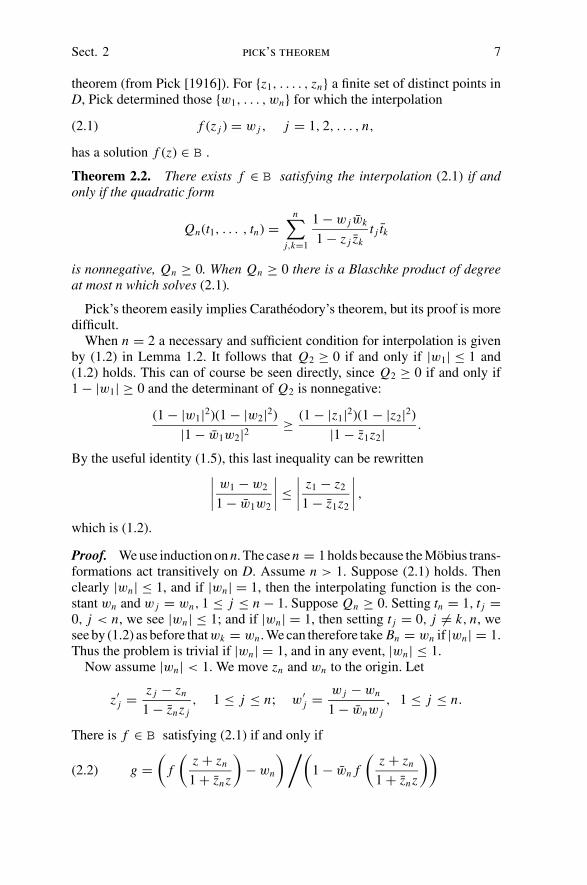
Sect. 2 pick’s theorem 7
theorem (from Pick [1916]). For {z1, . . . . , zn} a finite set of distinct points inD, Pick determined those {w1, . . . , wn} for which the interpolation
f (z j ) = w j , j = 1, 2, . . . , n,(2.1)
has a solution f (z) ∈ B .
Theorem 2.2. There exists f ∈ B satisfying the interpolation (2.1) if andonly if the quadratic form
Qn(t1, . . . , tn) =n∑
j,k=1
1 − w j wk
1 − z j zkt j tk
is nonnegative, Qn ≥ 0. When Qn ≥ 0 there is a Blaschke product of degreeat most n which solves (2.1).
Pick’s theorem easily implies Caratheodory’s theorem, but its proof is moredifficult.
When n = 2 a necessary and sufficient condition for interpolation is givenby (1.2) in Lemma 1.2. It follows that Q2 ≥ 0 if and only if |w1| ≤ 1 and(1.2) holds. This can of course be seen directly, since Q2 ≥ 0 if and only if1 − |w1| ≥ 0 and the determinant of Q2 is nonnegative:
(1 − |w1|2)(1 − |w2|2)
|1 − w1w2|2 ≥ (1 − |z1|2)(1 − |z2|2)
|1 − z1z2| .
By the useful identity (1.5), this last inequality can be rewritten∣∣∣∣
w1 − w2
1 − w1w2
∣∣∣∣ ≤
∣∣∣∣
z1 − z2
1 − z1z2
∣∣∣∣ ,
which is (1.2).
Proof. We use induction on n. The case n = 1 holds because the Mobius trans-formations act transitively on D. Assume n > 1. Suppose (2.1) holds. Thenclearly |wn| ≤ 1, and if |wn| = 1, then the interpolating function is the con-stant wn and w j = wn, 1 ≤ j ≤ n − 1. Suppose Qn ≥ 0. Setting tn = 1, t j =0, j < n, we see |wn| ≤ 1; and if |wn| = 1, then setting t j = 0, j �= k, n, wesee by (1.2) as before that wk = wn . We can therefore take Bn = wn if |wn| = 1.Thus the problem is trivial if |wn| = 1, and in any event, |wn| ≤ 1.
Now assume |wn| < 1. We move zn and wn to the origin. Let
z′j = z j − zn
1 − znz j, 1 ≤ j ≤ n; w′
j = w j − wn
1 − wnw j, 1 ≤ j ≤ n.
There is f ∈ B satisfying (2.1) if and only if
g =(
f
(z + zn
1 + znz
)
− wn
) /(
1 − wn f
(z + zn
1 + znz
))
(2.2)
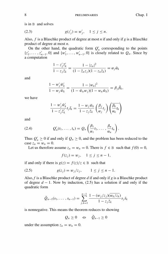
8 preliminaries Chap. I
is in B and solves
g(z′j ) = w′
j , 1 ≤ j ≤ n.(2.3)
Also, f is a Blaschke product of degree at most n if and only if g is a Blaschkeproduct of degree at most n.
On the other hand, the quadratic form Q′n corresponding to the points
{z′1, . . . , z′
n−1, 0} and {w′1, . . . , w
′n−1, 0} is closely related to Qn . Since by
a computation
1 − z′j z
′k
1 − z j zk= 1 − |zn|2
(1 − znz j )(1 − zn zk)= α j αk
and
1 − w′j w
′k
1 − w j wk= 1 − |wn|2
(1 − wnw j )(1 − wnwk)= β j βk,
we have
1 − w′j w
′k
1 − z′j z
′k
t j tk = 1 − w j wk
1 − z j zk
(β j
α jt j
) (βk
αktk
)
and
Q′n(t1, . . . , tn) = Qn
(β1
α1
t1, . . . ,βn
αntn
)
.(2.4)
Thus Q′n ≥ 0 if and only if Qn ≥ 0, and the problem has been reduced to the
case zn = wn = 0.Let us therefore assume zn = wn = 0. There is f ∈ B such that f (0) = 0,
f (z j ) = w j , 1 ≤ j ≤ n − 1,
if and only if there is g(z) = f (z)/z ∈ B such that
g(z j ) = w j/z j , 1 ≤ j ≤ n − 1.(2.5)
Also, f is a Blaschke product of degree d if and only if g is a Blaschke productof degree d − 1. Now by induction, (2.5) has a solution if and only if thequadratic form
Qn−1(s1, . . . , sn−1) =n−1∑
j,k=1
1 − (w j/z j )(wk/zk)
1 − z j zks j sk
is nonnegative. This means the theorem reduces to showing
Qn ≥ 0 ⇔ Qn−1 ≥ 0
under the assumption zn = wn = 0.
Sect. 2 pick’s theorem 9
Because zn = wn = 0, we have
Qn(t1, . . . , tn) = |tn|2 + 2 Ren−1∑
j=1
t j tn +n−1∑
j,k=1
1 − w j wk
1 − z j zkt j tk .
Completing the square relative to tn gives
Qn(t1, . . . , tn) =∣∣∣∣∣tn +
n−1∑
j=1
t j
∣∣∣∣∣
2
+n−1∑
j,k=1
(1 − w j wk
1 − z j zk− 1
)
t j tk .
Now
1 − w j wk
1 − z j zk− 1 = z j zk − w j wk
1 − z j zk= 1 − (w j/z j )(wk/zk)
1 − z j zkz j zk .
Hence
Qn(t1, . . . , tn) =∣∣∣∣∣
n∑
j=1
t j
∣∣∣∣∣
2
+ Qn−1(z1t1, . . . , zn−1tn−1).(2.6)
Thus Qn−1 ≥ 0 implies Qn ≥ 0, and setting tn = − ∑n−11 t j , we see also that
Qn ≥ 0 implies Qn−1 ≥ 0.
Corollary 2.3. Suppose Qn ≥ 0. Then (2.1) has a unique solution f (z) ∈ Bif and only if det (Qn) = 0. If det(Qn) = 0 and m < n is the rank of Qn, thenthe interpolating function is a Blaschke product of degree m. Conversely, if aBlaschke product of degree m < n satisfies (2.1), then Qn has rank m.
Proof. If |wn| = 1 the whole thing is very trivial because then Qn = 0,m = 0, and Bn = wn . So we may assume |wn| < 1. We may then supposezn = wn = 0, because by (2.4), Qn and Q′
n have the same rank, while by(2.2), the original problem has a unique solution if and only if the adjustedproblem (2.3) has a unique solution. Also (2.3) can be solved with a Blaschkeproduct of degree m if and only if (2.1) can be also.
So we assume zn = wn = 0. Then (2.1) has a unique solution if and only if(2.5) has a unique solution; and (2.1) can be solved with a Blaschke product ofdegree m − 1. Consequently, by induction, all assertions of the corollary willbe proved when we show
rank(Qn) = 1 + rank(Qn−1).(2.7)
Writing Qn−1 = (a j,k), we have
Qn =
⎡
⎢⎢⎢⎣
------------
1
1 + z j zka j,k...1- - - - - - - - - - - - - - -
1 · · · 1 1
⎤
⎥⎥⎥⎦
,
10 preliminaries Chap. I
which has the same rank as⎡
⎢⎢⎢⎣
------------
0
z j zka j,k...0- - - - - - - - - -
1 · · · 1
⎤
⎥⎥⎥⎦
,
and the rank of this matrix is 1 + rank(Qn−1).
Corollary 2.4. Suppose Qn ≥ 0 and det (Qn) > 0. Let z ∈ D, z �= z j , j =1, 2, . . . , n. The set of values
W = { f (z) : f ∈ B , f (z j ) = w j , 1 ≤ j ≤ n}is a nondegenerate closed disc contained in D. If f ∈ B , and if f satisfies (2.1),then f (z) ∈ ∂W if and only if f is a Blaschke product of degree n. Moreover, ifw ∈ ∂W , there is a unique solution to (2.1) in B which also solves f (z) = w.
Proof. We may again suppose zn = wn = 0. Then det(Qn−1) > 0 by (2.7).By induction,
W = {g(z) : g ∈ B , g(z j ) = w j/z j , 1 ≤ j ≤ n − 1}is a closed disc contained in D. But then W = {zζ : ζ ∈ W } is also a closeddisc. Since w ∈ ∂W if and only if w/z ∈ ∂W , the other assertions follow byinduction.
We shall return to this topic in Chapter IV.
3. Poisson Integrals
Let u(z) be a continuous function on the closed unit disc D. If u(z) isharmonic on the open disc D, that is, if
�u = ∂ 2u
∂x2+ ∂ 2u
∂y2= 0,
then u(z) has the mean value property
u(0) = 1
2π
∫ 2π
0
u(eiθ ) dθ.
Let z0 = reiθ0 be a point in D. Then there is a similar representation formulafor u(z0), obtained by changing variables through a Mobius transformation.Let τ (z) = (z − z0)/(1 − z0z). The unit circle ∂D is invariant under τ , and wemay write τ (eiθ ) = eiϕ . Differentiation now gives
dϕ
dθ= 1 − |z0|2
|eiθ − z0|2 = 1 − r2
1 − 2r cos(θ − θ0) + r2= Pz0
(θ ).(3.1)
Sect. 3 poisson integrals 11
This function Pz0(θ ) is called the Poisson kernel for the point z0 ∈ D. Since
u(τ−1(z)) is another function continuous on D and harmonic on D, the changeof variables yields
u(z0) = u(τ−1(0)) = 1
2π
∫ 2π
0
u(eiθ )Pz0(θ ) dθ.
This is the Poisson integral formula.Notice that the Poisson kernel Pz(θ ) also has the form
Pz(θ ) = Reeiθ + z
eiθ − z,
so that for eiθ fixed, Pz(θ ) is a harmonic function of z ∈ D. Hence the functiondefined by
u(z) = 1
2π
∫Pz(θ ) f (θ ) dθ(3.2)
is harmonic on D whenever f (θ ) ∈ L1(∂D). Since Pz(θ ) is also a continuousfunction of θ , we get a harmonic function from (3.2) if we replace f (θ ) dθ
by a finite measure dμ(θ ) on ∂D. The extreme right side of (3.1) shows thatthe Poisson integral formula may be interpreted as a convolution. If z = reiθ0 ,then
Pz(θ ) = Pr (θ0 − θ )
and (3.2) takes the form
u(z) = 1
2π
∫Pr (θ0 − θ ) f (θ ) dθ = (Pr ∗ f )(θ0).
This reflects the fact that the space of harmonic functions on D is invariantunder rotations.
Map D to the upper half plane H by w → z(w) = i(1 − w)/(1 + w). Fixw0 ∈ D and let z0 = z(w0) be its image in H . Our map sends ∂D to � ∪ {∞},so that if w = eiθ ∈ ∂D, and w �= −1, then z(w) = t ∈ �. Differentiation nowgives
1
2πPw0
(θ )dθ
dt= 1
π
y0
(x0 − t)2 + y20
= Pz0(t), z0 = x0 + iy0.
The right side of this equation is the Poisson kernel for the upper half plane,Pz0
(t) = Py0(x0 − t). (The notation is unambiguous because z0 ∈ H but
y0 �∈ H .) Pulling the Poisson integral formula for D over to H , we seethat
u(z) =∫
Pz(t)u(t) dt =∫
Py(x − t)u(t) dt(3.3)
12 preliminaries Chap. I
whenever the function u(z) is continuous on H ∪ {∞} and harmonic on H .When t ∈ � is fixed, the Poisson kernel for the upper half plane is a harmonicfunction of z, because
Pz(t) = 1
πIm
(1
t − z
)
.
From its defining formula we see that Pz(t) ≤ cz/(1 + t2), where cz is a con-stant depending on z. Consequently, if 1 ≤ q ≤ ∞, then Pz(t) ∈ L2(�), andthe function
u(z) =∫
Pz(t) f (t) dt(3.4)
is harmonic on H whenever f (t) ∈ L p(�), 1 ≤ p ≤ ∞. Moreover, sincePz(t) is a continuous function of t, (3.4) will still produce a harmonic functionu(z) if f (t) dt is replaced by a finite measure dμ(t) or by a positive measuredμ(t) such that
∫1
1 + t2dμ(t) < ∞
(so that∫
Pz(t) dμ(t) converges).Now let f (t) be the characteristic function of an interval (t1, t2). The resulting
harmonic function
ω(z) =∫ t2
t1
Py(x − t) dt,
called the harmonic measure of the interval, can be explicitly calculated. Weget
ω(z) = 1
πarg
(z − t2z − t1
)
= α
π,
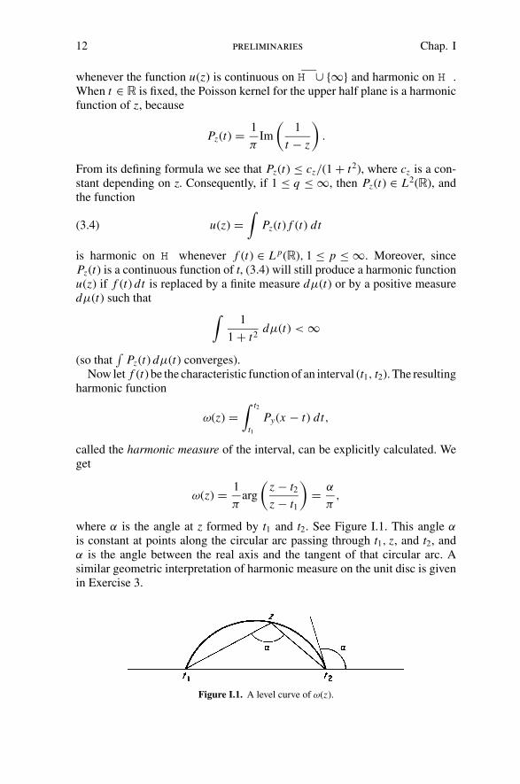
where α is the angle at z formed by t1 and t2. See Figure I.1. This angle α
is constant at points along the circular arc passing through t1, z, and t2, andα is the angle between the real axis and the tangent of that circular arc. Asimilar geometric interpretation of harmonic measure on the unit disc is givenin Exercise 3.
Figure I.1. A level curve of ω(z).

Sect. 3 poisson integrals 13
The Poisson integral formula for the upper half plane can be written as aconvolution
u(z) =∫
Py(x − t) f (t) dt = (Py ∗ f )(t).
This follows from the formula defining the Poisson kernel, and reflects thefact that under the translations z → z + x0, x0 real, the space of harmonicfunctions on H is invariant. The harmonic functions are also invariant underthe dilations z → az, a > 0, and accordingly we have
Py(t) = (1/y)P1(t/y),
which means Py is homogeneous of degree −1 in y. The Poisson kernel hasthe following properties, illustrated in Figure I.2:
(i) Py(t) ≥ 0,∫
Py(t) dt = 1.(ii) Py is even, Py(−t) = Py(t).
(iii) Py is decreasing in t > 0.(iv) Py(t) ≤ 1/πy.
For any δ > 0,
(v) sup|t |>δ Py(t) → 0 (y → 0).
(vi)∫|t |>δ
Py(t) dt → 0 (y → 0).
Moreover, {Py} is a semigroup.
(vii) Py1∗ Py2
= Py1+y2.
Figure I.2. The Poisson kernels P1/4 and P1/8.
The first six properties are obvious from the definition of Py(t), and properties(iv)–(vi) also follow from the homogeneity in y. Property (vii) means that ifu(z) is a harmonic function given by (3.4), then u(z + iy1) can be computed
14 preliminaries Chap. I
from u(t + iy1), t ∈ �, by convolution with Py . To prove (vii), consider theharmonic function u(x + iy) = Py1+y(x). This function extends continuously
to H ∪ {∞}. Consequently by (3.3),
Py1+y2(x) =
∫Py2
(x − t)u(t) dt = (Py1∗ Py2
)(x).
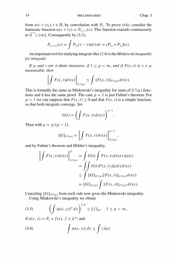
An important tool for studying integrals like (3.4) is the Minkowski inequalityfor integrals:
If μ and v are σ -finite measures, if 1 ≤ p < ∞, and if F(x, t) is ν × μ
measurable, then∥∥∥∥
∫F(x, t)dν(x)
∥∥∥∥
L p(μ)
≤∫
‖F(x, t)‖L p(μ) dν(x).
This is formally the same as Minkowski’s inequality for sums of L p(μ) func-tions and it has the same proof. The case p = 1 is just Fubini’s theorem. Forp > 1 we can suppose that F(x, t) ≥ 0 and that F(x, t) is a simple function,so that both integrals converge. Set
G(t) =(∫
F(x, t) dν(x)
)p−1
.
Then with q = p/(p − 1),
‖G‖Lq (μ) =∥∥∥∥
∫F(x, t) dν(x)
∥∥∥∥
p−1
L p(μ)
,
and by Fubini’s theorem and Holder’s inequality,∥∥∥∥
∫F(x, t) dν(x)
∥∥∥∥
p
L p(μ)
=∫
G(t)∫
F(x, t) dν(x) dμ(t)
=∫ ∫
G(t)F(x, t) dμ(t) dν(x)
≤∫
‖G‖Lq (μ)‖F(x, t)‖L p(μ) dν(x)
= ‖G‖Lq (μ)
∫‖F(x, t)‖L p(μ) dν(x).
Canceling ‖G‖Lq (μ) from each side now gives the Minkowski inequality.Using Minkowski’s inequality we obtain
(∫|u(x, y)|p dx
)1/p
≤ ‖ f ‖p, 1 ≤ p < ∞,(3.5)
if u(x, y) = Py ∗ f (x), f ∈ L p; and∫
|u(x, y)| dx ≤∫
| dμ|(3.6)

Sect. 3 poisson integrals 15
if u(x, y) = Py ∗ μ = ∫Py(x − t) dμ(t), where μ is a finite measure on �.
For p = ∞ the analog of (3.5), supx |u(x, y)| ≤ ‖ f ‖∞, is trivial from property(i) of Py(t).
Theorem 3.1. (a) If 1 ≤ p < ∞ and if f (x) ∈ L p, then
‖Py ∗ f − f ‖p → 0 (y → 0).
(b) When f (x) ∈ L∞, Py ∗ f converges weak-star to f (x).(c) If dμ is a finite measure on �, the measures (Py ∗ μ)(x) dx converge
weak-star to dμ.(d) When f (x) is bounded and uniformly continuous on �, Py ∗ f (x) con-
verges uniformly to f (x).
Statement (b) means that for all g ∈ L1,∫
g(x)(Py ∗ f )(x) dx →∫
f (x)g(x) dx (y → 0).
Statement (c) has a similar meaning:∫
g(x)(Py ∗ μ)(x) dx →∫
g(x) dμ(x) (y → 0),
for all g ∈ C0(�), the continuous functions vanishing at ∞. It follows fromTheorem 3.1 that f ∈ L p is uniquely determined by the harmonic functionu(z) = Py ∗ f (x) and that a measure μ is determined by its Poisson integralPy ∗ μ. Note also that by (a) or (b)
limy→0
‖Py ∗ f ‖p = ‖ f ‖p, 1 ≤ p ≤ ∞.
By (3.5) and property (vii), the function ‖Py ∗ f ‖p is monotone in y.Besides Minkowski’s inequality, the main ingredient of the proof of the the-
orem is the continuity of translations on L p, 1 ≤ p < ∞: If fx (t) = f (t − x),then ‖ fx − f ‖p → 0(x → 0). (To prove this approximate f in L p norm by afunction in C0(�).) The translations are not continuous on L∞ nor are theyon the space of finite measures; that is why we have weaker assertions in(b) and (c). The translations are of course continuous on the space of uni-formly continuous functions, and for this reason (d) holds.
Proof. Let f ∈ L p, 1 ≤ p ≤ ∞. When p = ∞ we suppose in addition thatf is uniformly continuous. Then
Py ∗ f (x) − f (x) =∫
Py(t)( f (x − t) − f (x)) dt.
Minkowski’s inequality gives
‖Py ∗ f − f ‖p ≤∫
Py(t)‖ ft − f ‖p dt,

16 preliminaries Chap. I
when p < ∞, because Py ≥ 0. The same inequality is trivial when p = ∞.For δ > 0, we now have
‖Py ∗ f − f ‖p ≤∫
|t |≤δ
Py(t)‖ ft − f ‖p dt +∫
|t |>δ
Py(t)‖ ft − f ‖p dt.
Since∫
Py(t) dt = 1, continuity of translations shows that∫|t |≤δ
is small pro-
vided δ is small. With δ fixed,∫
|t |>δ
≤ 2‖ f ‖p
∫
|t |>δ
Py(t) dt → 0 (y → 0)
by property (vi) of the Poisson kernel. That proves (a) and (d). By Fubini’stheorem, parts (b) and (c) follow from (a) and (d), respectively.
Corollary 3.2. Assume f (x) is bounded and uniformly continuous, and let
u(x, y) ={
(Py ∗ f )(x), y > 0,
f (x), y = 0.
Then u(x, y) is harmonic on H and continuous on H .
This corollary follows from (d). We also need the local version of thecorollary.
Lemma 3.3. Assume f (x) ∈ L p, 1 ≤ p ≤ ∞, and assume f is continuousat x0. Let u(x, y) = Py ∗ f (x). Then
lim(x,y)→x0
u(x, y) = f (x0).
Proof. We have
|u(x, y) − f (x0)| ≤∫
|t |<δ
Py(t)| f (x − t) − f (x0)| dt +∫
|t |≥δ
.
With δ small and |x − x0| small,∫|t |<δ
is small. With δ fixed,∫|t |≥δ
tends to
zero with y.
Notice that the convergence is uniform on a subset E ⊂ � provided thecontinuity of f is uniform over x0 ∈ E and provided | f (x0)| is bounded on E.
It is important that the Poisson integrals of L p functions and measures arecharacterized by the norm inequalities like (3.5) and (3.6). The proof of thisin the upper half plane requires the following lemma.
Lemma 3.4. If u(z) is harmonic on H and bounded and continuous onH then
u(z) =∫
Py(x − t)u(t) dt.

Sect. 3 poisson integrals 17
Proof. The lemma is not a trivial consequence of the definition of Pz(t),because u(z) may not be continuous at ∞. But let
U (z) = u(z) −∫
Py(x − t)u(t) dt.
Then U (z) is harmonic on H , and bounded and continuous on H , and U ≡ 0on �, by Lemma 3.3. Set
V (z) ={
U (z), y ≥ 0,
−U (z), y < 0.
Then V is a bounded harmonic function on the complex plane, because Vhas the mean value property over small discs. By Liouville’s theorem, V isconstant; V (z) = V (0) = 0. Hence U (z) = 0 and the lemma is proved.
Theorem 3.5. Let u(z) be a harmonic function on the upper half plane H .Then
(a) If 1 < p ≤ ∞, u is the Poisson integral of a function in L p if and onlyif
supy
∫‖u(x + y)‖L p(dx) < ∞.(3.7)
(b) u(z) is the Poisson integral of a finite measure on � and only if
supy
∫|u(x + iy)| dx < ∞.(3.8)
(c) u(z) is positive if and only if
u(z) = cy +∫
Py(x − t) dμ(t),
where
c ≥ 0, μ ≥ 0, and∫
dμ(t)
1 + t2< ∞.
Proof. We have already noted that (3.7) and (3.8) are necessary conditionsbecause of Minkowski’s inequality. Suppose u(z) satisfies (3.7) or (3.8). Thenwe have the estimate
|u(z)| ≤(
2
πy
)1/p
supη>0
‖u(x, η)‖L p(dx),(3.9)

18 preliminaries Chap. I
which we now prove: Write ζ = ξ + iη. Then by Holder’s inequality,
|u(z)| = 1
πy2
∣∣∣
∫∫
�(z,y)
u(ζ ) dξ dη
∣∣∣
≤(
1
πy2
∫∫
�(z,y)
|u(ζ )|p dξ dη
)1/p
≤(
1
πy2
∫ 2y
0
∫ ∞
−∞|u(ξ + iη)|p dξ dη
)1/p
≤(
2
πy
)1/p
supη>0
(∫|u(ξ + iη)|p dξ
)1/p
.
The estimate (3.9) tells us u(z) is bounded on y > yn > 0, and Lemma 3.4then gives
u(z + iyn) =∫
Py(x − t)u(t + iyn) dt.
Let yn decrease to 0. If 1 < p ≤ ∞, the sequence fn(t) = u(t + iyn) isbounded in L p. By the Banach–Alaoglu theorem, which says the closed unitball of the dual of a Banach space is compact in the weak-star topology,{ fn} has a weak-star accumulation point f ∈ L p. Since Poisson kernels are inLq , q = p/(p − 1), we have
u(z) = limn
u(z + iyn) = limn
∫Py(x − t) fn(t) dt =
∫Py(x − t) f (t) dt.
The proof of (b) is the same except that now the measures u(t + iyn) dt ,which have bounded norms, converge weak-star to a finite measure on �.
The easiest proof of (c) involves mapping H back onto D, using the analogof (b) for harmonic functions on the disc, and then returning to H . A harmonicfunction u(z) on D is the Poisson integral of a finite measure ν on ∂D if andonly if supr
∫ |u(reiθ )| dθ < ∞. The measure ν is then a limit of the measuresu(reiθ )dθ/2π in the weak-star topology on measures on ∂D. If u(z) ≥ 0, thenthe measures u(reiθ ) dθ are positive and bounded since
1
2π
∫u(reiθ ) dθ = u(0),
and so the limit ν exists and ν is a positive measure. That proves the discversion of (c). Now map D to H by w → z(w) = i(1 − w)/(1 + w). Theharmonic function u on H is positive if and only if the harmonic functionu(z(w)), which is positive, is the Poisson integral of a positive measure v on∂D. Consider first the case when v is supported on the point w = −1, which
Sect. 4 hardy–littlewood maximal function 19
corresponds to z = ∞. Then
u(z(w)) = ν({−1})Pw(−1) = ν({−1})1 − |w|2|1 + w|2
= ν({−1}) Im z = ν({−1})y.
Now assumeν({−1}) = 0. The map z(w) movesν onto a finite positive measureν on �, and for t = z(eiθ )
Pw(θ ) = π (1 + t2)Pz(t).
In this case we have
u(z) =∫
Py(x − t) dμ(t),
where
μ = π (1 + t2)ν.
The general case is the sum of the two special cases already discussed.
Part c) of Theorem 3.5 is known as Herglotz’s theorem. The results in thissection also hold in D, where they are easier to prove, when we write
u(reiθ ) = 1
2π
∫Pr (θ − ϕ) f (ϕ) dϕ,
Pr (θ − ϕ) = 1 − r2
1 − 2r cos(θ − ϕ) + r2, z = reiθ .
Most of these results also hold if {Py(t)} is replaced by some other approxi-mate identity. Suppose {ϕy(t)}y>0 is a family of integrable functions on � suchthat
(a)∫
ϕy(t) dt = 1,(b) ‖ϕy‖1 ≤ M ,
and such that for any δ > 0,
(c) limy→0 sup|t |>δ |ϕy(t)| = 0,
(d) limy→0
∫|t |>δ
|ϕy(t)| dt = 0.
Then the reader can easily verify that Theorem 3.1 and its corollary hold forϕy ∗ f in place of Py ∗ f .
4. Hardy–Littlewood Maximal Function
To each function f on � we associate two auxiliary functions that respectivelymeasure the size of f and the behavior of the Poisson integral of f. The first

20 preliminaries Chap. I
auxiliary function can be defined whenever f is a measurable function on anymeasure space (X, μ). This is the distribution function
m(λ) = μ({x ∈ X : | f (x)| > λ}),defined for λ > 0. The distribution function m(λ) is a decreasing function of λ,and it determines the L p norms of f . If f ∈ L∞, then m(λ) = 0 for λ ≥ ‖ f ‖∞,and m(λ) > 0 for λ < ‖ f ‖∞; and so we have
‖ f ‖∞ = sup{λ : m(λ) > 0}.Lemma 4.1. If (X, μ) is a measure space, if f (x) is measurable, and if0 < p < ∞, then
∫| f |p dμ =
∫ ∞
0
pλp−1m(λ) dλ.(4.1)
Proof. We may assume f vanishes except on a set of σ -finite measure,because otherwise both sides of (4.1) are infinite. Then Fubini’s theoremshows that both sides of (4.1) equal the product measure of the ordinate set{(x, λ) : 0 < λ < | f (x)|p}. That is,
∫| f |p dμ =
∫∫ | f |
0
pλp−1 dλ dμ =∫ ∞
0
pλp−1μ(| f | > λ) dλ
=∫ ∞
0
pλp−1m(λ) dλ.
We shall also need a simple estimate of m(λ) known as Chebychev’s in-equality. Let f ∈ L p, 0 < p < ∞ and let
Eλ = {x ∈ X : | f (x)| > λ},so that μ(Eλ) = m(λ). Chebychev’s inequality is
m(λ) ≤ ‖ f ‖pp/λ
p.
It follows from the observation that
λpμ(Eλ) ≤∫
Eλ
| f |p dμ ≤ ‖ f ‖pp.
A function f that satisfies
m(λ) ≤ A/λp
is called a weak L p function. Thus Chebychev’s inequality states that everyL p function is a weak L p function. The function |x log x |−1 on [0, 1] is not inL1, but it satisfies m(λ) = o(1/λ) (λ → ∞), and so it is weak L1.

Sect. 4 hardy–littlewood maximal function 21
The other auxiliary function we shall define only for functions on �. RecallLebesgue’s theorem that if f (x) is locally integrable on �, then
limh→0k→0
1
h + k
∫ x+k
x−hf (t) dt = f (x)(4.2)
for almost every x ∈ �. To make Lebesgue’s theorem quantitative we replacethe limit in (4.2) by the supremum, and we put the absolute value insidethe integral. Write |I | for the length of an interval I. The Hardy–Littlewoodmaximal function of f is
M f (x) = supx∈I
1
|I |∫
I| f (t)| dt
for f locally integrable on �. Now if f ∈ L p, p ≥ 1, then M f (x) < ∞ almosteverywhere. This follows from Lebesgue’s theorem, but we shall soon see adifferent proof in Theorem 4.3 below. The important thing about Mf is that itmajorizes many other functions associated with f.
Theorem 4.2. For α > 0 and t ∈ �, let �α(t) be the cone in H with vertext and angle 2 arctan α, as shown in Figure I.3,
�α(t) = {(x, y) : |x − t | < αy, 0 < y < ∞}.Let f ∈ L1(dt/(1 + t2)) and let u(x, y) be the Poisson integral of f (t),
u(x, y) =∫
Py(s) f (x − s) ds.
Then
sup�α(t)
|u(x, y)| ≤ Aα M f (t), t ∈ �,(4.3)
where Aα is a constant depending only on α.
Figure I.3. The cone �α(t), α = 23.
The condition f ∈ L1(dt/(1 + t2)) merely guarantees that∫
Py(s) f (x − s) dsconverges.

22 preliminaries Chap. I
Proof. We may assume t = 0. Let us first consider the points (0, y) on theaxis of the cone �α(0). Then
u(0, y) =∫
Py(s) f (s) ds,
and the kernel Py(s) is a positive even function which is decreasing for positives. That means Py(s) is a convex combination of the box kernels (1/2h)χ(−h,h)(s)that arise in the definition of Mf. Take step functions hn(s), which are alsononnegative, even, and decreasing on s > 0, such that hn(s) increases with nto Py(s). Then hn(s) has the form
N∑
j=1
a jχ(−x j ,x j )(s)
with a j ≥ 0, and∫
hn ds = ∑j 2x j a j ≤ 1. See Figure I.4. Hence
∣∣∣∣
∫hn(s) f (s) ds
∣∣∣∣ ≤
∫hn(s)| f (s)| ds ≤
N∑
j=1
2x j a j1
2x j
∫ x j
−x j
| f (s)| ds ≤ M f (0).
Then by monotone convergence
|u(0, y)| ≤∫
Py(s)| f (s)| ds ≤ M f (0).
Figure I.4. Py(s) and its approximation hn(s), which is a positive combination of box kernels(1/2x j )χ(−x j ,x j )(s).
Now fix (x, y) ∈ �α(0). Then |x | < αy, and Py(x − s) is majorized by a pos-itive even function ψ(s), which is decreasing on s > 0, such that
∫ψ(s) ds ≤ Aα = 1 + 2α
π.
Sect. 4 hardy–littlewood maximal function 23
The function is ψ(s) = sup{Py(x − t) : |t | > s}. Approximating ψ(s) frombelow by step functions hn(s) just as before, we have
∫ψ(s)| f (s)| ds ≤ Aα M f (0)
and
|u(x, y)| ≤∫
ψ(s)| f (s)| ds ≤ Aα M f (0),
which is (4.3).
Theorem 4.2 is, with the same proof, true for Poisson integrals of functionson ∂D, where the cone is replaced by the region
�α(eiϕ) ={
z :|eiϕ − z|1 − |z| < α, |z| < 1
}
, α > 1,
which is asymptotic, as z → eiϕ , to an angle with vertex eiϕ . The theorem isquite general. The proof shows it is true with Py(x − s) replaced by any kernelϕy(x − s) which can be dominated by a positive, even function ψ(s), dependingon (x, y), provided that ψ is decreasing on s > 0 and that
∫ψ(s) ds ≤ Aα
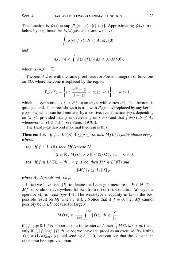
whenever (x, y) ∈ �α(t) (see Stein, [1970]).The Hardy–Littlewood maximal theorem is this:
Theorem 4.3. If f ∈ L p(�), 1 ≤ p ≤ ∞, then M f (t) is finite almost every-where.
(a) If f ∈ L1(�), then Mf is weak L1,
|{t ∈ � : M f (t) > λ}| ≤ (2/λ)‖ f ‖1, λ > 0.
(b) If f ∈ L p(�), with 1 < p ≤ ∞, then M f ∈ L p(�) and
‖M f ‖p ≤ Ap‖ f ‖p,
where Ap depends only on p.
In (a) we have used |E | to denote the Lebesgue measure of E ⊂ �. ThatM f < ∞ almost everywhere follows from (a) or (b). Condition (a) says theoperator Mf is weak-type 1–1. The weak-type inequality in (a) is the bestpossible result on Mf when f ∈ L1. Notice that if f ≡ 0, then Mf cannotpossibly be in L1, because for large x
M f (x) ≥ 1
|4x |∫ 3x
−x| f (t)| dt ≥ c
|x |if ‖ f ‖1 �= 0. If f is supported on a finite interval I, then
∫I M f (t)dt < ∞ if and
only if∫
I | f | log+ | f | dt < ∞; we leave the proof as an exercise. By lettingf (t) = (1/h)χ(0,h)(t), and sending h → 0, one can see that the constant in(a) cannot be improved upon.
24 preliminaries Chap. I
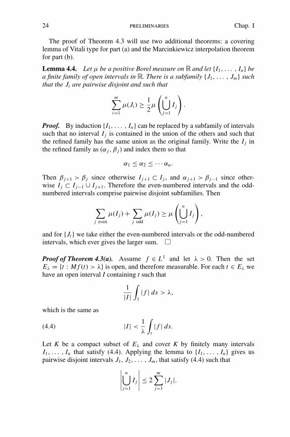
The proof of Theorem 4.3 will use two additional theorems: a coveringlemma of Vitali type for part (a) and the Marcinkiewicz interpolation theoremfor part (b).
Lemma 4.4. Let μ be a positive Borel measure on � and let {I1, . . . , In} bea finite family of open intervals in �. There is a subfamily {J1, . . . , Jm} suchthat the Ji are pairwise disjoint and such that
m∑
i=1
μ(Ji ) ≥ 1
2μ
(n⋃
j=1
I j
)
.
Proof. By induction {I1, . . . , In} can be replaced by a subfamily of intervalssuch that no interval I j is contained in the union of the others and such thatthe refined family has the same union as the original family. Write the I j inthe refined family as (α j , β j ) and index them so that
α1 ≤ α2 ≤ · · · αn.
Then β j+1 > β j since otherwise I j+1 ⊂ I j , and α j+1 > β j−1 since other-wise I j ⊂ I j−1 ∪ I j+1. Therefore the even-numbered intervals and the odd-numbered intervals comprise pairwise disjoint subfamilies. Then
∑
j even
μ(I j ) +∑
j odd
μ(I j ) ≥ μ
(n⋃
j=1
I j
)
,
and for {Ji } we take either the even-numbered intervals or the odd-numberedintervals, which ever gives the larger sum.
Proof of Theorem 4.3(a). Assume f ∈ L1 and let λ > 0. Then the setEλ = {t : M f (t) > λ} is open, and therefore measurable. For each t ∈ Eλ wehave an open interval I containing t such that
1
|I |∫
1
| f | ds > λ,
which is the same as
|I | <1
λ
∫
t| f | ds.(4.4)
Let K be a compact subset of Eλ and cover K by finitely many intervalsI1, . . . , In that satisfy (4.4). Applying the lemma to {I1, . . . , In} gives uspairwise disjoint intervals J1, J2, . . . , Jm , that satisfy (4.4) such that
∣∣∣∣∣
n⋃
j=1
I j
∣∣∣∣∣≤ 2
m∑
j=1
|Jj |.
Sect. 4 hardy–littlewood maximal function 25
Then
|K | ≤∣∣∣∣∣
n⋃
i=1
I j
∣∣∣∣∣≤ 2
∑
j
1
λ
∫
J j
| f | ds ≤ 2
λ
∫| f | ds.
Letting |K | increase to |Eλ| gives us part (a).
The proof of part (b) depends on the interpolation theorem of Marcinkiewicz.
Theorem 4.5. Let (X, μ) and (Y, ν) be measure spaces, and let 1 < p1 ≤ ∞.Suppose T is a mapping from L1(X, μ) + L p1 (X, μ) to v-measurable functionssuch that
(i) |T ( f + g)(y)| ≤ |T f (y)| + |T g(y)|;(ii) ν({y : |T f (y)| > λ}) ≤ (A0/λ)‖ f ‖1, f ∈ L1;
(iii) ν({y : |T f (y)| > λ}) ≤ ((A1/λ)‖ f ‖p1)p1, f ∈ L p1 ;
(when p1 = ∞ we assume instead that
‖T f ‖∞ ≤ A1‖ f ‖∞).
Then for 1 < p < p1,
‖T f ‖p ≤ Ap‖ f ‖p, f ∈ L p,
where Ap depends only on A0, A1, p, and p1.
The hypothesis that the domain of T is L1(X, μ) + L p1 (X, μ) is just adevice to make sure Tf is defined when f ∈ L p, 1 ≤ p ≤ p1. For f ∈ L p,write f = f χ| f |>1 + f χ| f |≤1 = f0 + f1. Then | f0| ≤ | f |p ∈ L1 and | f1| ≤| f |p/p1 ∈ L p1 . Before proving the theorem, let us use it to prove the remainingpart (b) of the Hardy–Littlewood maximal theorem.
Proof of Theorem 4.3(b). In this case the measure spaces are both (�, dx).The operator M clearly satisfies the subadditivity condition (i). Condition(ii) we proved as part (a) of the Hardy–Littlewood theorem. We take p1 = ∞and condition (iii) holds with A1 = 1. The Marcinkiewicz theorem then tellsus
‖M f ‖p ≤ Ap‖ f ‖p, 1 < p ≤ ∞which is the assertion in part (b) of Theorem 4.3. It of course follows thatM f < ∞ almost everywhere.
Proof of Theorem 4.5. Fix f ∈ L p, 1 < p < p1, and, λ > 0. Let
Eλ = {y : |T f (y)| > λ}.We are going to get a tight grip on ν(Eλ) and then use Lemma 4.1 to estimate‖T f ‖p. The clever Marcinkiewicz idea is to split f at λ/2A1. Write
f0 = f χ{x :| f (x)|>λ/2A1}, f1 = f χ{x :| f (x)|≤λ/2A1}.

26 preliminaries Chap. I
Then |T f (y)| ≤ |T f0(y)| + |T f1(y)|, and Eλ ⊂ Bλ ∪ Cλ, where
Bλ = {y : |T f0(y)| > λ/2}, Cλ = {y : |T f1(y)| > λ/2}.Now by (ii) we have
ν(Bλ) ≤ 2A0
λ‖ f0‖1 ≤ 2
A0
λ
∫
| f |>λ/2A1
| f | dμ.
To estimate ν(Cλ) we consider two cases. If p1 = ∞, then ‖ f1‖∞ < λ/2A1
and by (iii) Cλ = ∅. (This explains the presence of A1 in the definitions of f0
and f1.) If p1 < ∞, we have by (iii)
ν(Cλ) ≤(
2
λA1‖ f1‖p1
)p1
≤ (2A1)p1
λp1
∫
| f |≤λ/2A1
| f |p1 dμ.
We bound ν(Eλ) by ν(Bλ) + ν(Cλ) and use Lemma 4.1. The case p1 = ∞ iseasier:
‖T f ‖pp =
∫ ∞
0
pλp−1ν(Eλ)dλ ≤∫ ∞
0
pλp−1
(2A0
λ
∫
| f |>λ/2A1
| f | dμ
)
dλ
≤ 2A0 p∫
| f |∫ 2A1| f |
0
λp−2dλ dμ = 2p A0 Ap−11 p
p − 1
∫| f |p dμ,
because p − 2 > −1. Hence T f ∈ L p. If p1 < ∞, we have the same thingplus an additional term bounding ν(Cλ):
‖T f ‖pp ≤
∫ ∞
0
pλp−1
(2A0
λ
∫
| f |>λ/2A1
| f | dμ
)
dλ
+∫ ∞
0
pλp−1 (2A1)p1
λp1
∫
| f |≤λ/2A1
| f |p1 dμ dλ.
The first integral we just estimated in the proof for p1 = ∞. The second integralis
(2A1)p1 p∫
| f |p1
∫ ∞
2A1| f |λp−p1−1 dλ dμ = (2A1)p p
p1 − p
∫| f |p dμ
because p − p1 − 1 < −1. Altogether this gives
‖T f ‖p ≤ Ap‖ f ‖p
with
App ≤ 2p Ap−1
1
(A0 p
p − 1+ A1 p
p1 − p
)
,
which proves the theorem.

Sect. 5 nontangential maximal function and fatou’s theorem 27
It is interesting that as p → 1, Ap ≤ A/(p − 1) for some constant A, and ifp1 = ∞, then limp→∞ Ap ≤ A1. For the maximal function we obtain
App = p2p+1/(p − 1).
Other splittings of f = f0 + f1 give more accurate estimates of the dependen-cies of Ap on A0 and A1 (see Zygmund [1968, Chapter XII]).
5. Nontangential Maximal Function and Fatou’s Theorem
Fix α > 0, and consider the cones
�α(t) = {z ∈ H : |x − t | < αy}, t ∈ �.
If u(z) is a harmonic function on H , the nontangential maximal function of uat t ∈ � is
u∗(t) = sup�α(t)
|u(z)|.
The value of u∗ depends on the parameter α, but since α has been fixed wewill ignore that distinction.
Theorem 5.1. Let u(z) be harmonic on H and let 1 ≤ p < ∞. Assume
supy
∫|u(x + iy)|p dx < ∞.
If p > 1, then u∗(t) ∈ L p, and
‖u∗‖pp ≤ Bp sup
y
∫|u(x + iy|p dx .(5.1)
If p = 1, then u∗ is weak L1, and
|{t : u∗(t) > λ} ≤ B1
λsup
y
∫|u(x + iy)| dx .(5.2)
The constants Bp depend only on p and α.
Proof. Let p > 1. Then u(z) is the Poisson integral of a function f (t) ∈L p(�), and
‖ f ‖p ≤ supy
(∫|u(x + iy)|p dx
)1/p
.
Theorem 4.2 says that u∗(t) ≤ Aα M f (t), and the Hardy–Littlewood theoremthen yields (5.1).

28 preliminaries Chap. I
If p = 1, we know only that u(z) is the Poisson integral of a finite measureμ on � and
∫|dμ| ≤ sup
y
∫|u(x + iy)| dx,
because μ is a weak-star limit of the measures u(x + iy) dx, y → 0. Define
M(dμ)(t) = supt∈I
(|μ|(I )/|I |).
The proof of Theorem 4.2 shows that u∗(t) ≤ Aα M(dμ)(t). And the proof ofpart (a) of Theorem 4.3 shows that M(dμ)(t) is weak L1 and
|{t : M(dμ)(t) > λ} ≤ 2
λ
∫d|μ|.
Therefore (5.2) holds in the case p = 1.
The nontangential maximal function u∗ will be more important to us thanthe Hardy–Littlewood maximal function Mf. The next corollary is stated toemphasize the strength of Theorem 5.1.
Corollary 5.2. If u(z) is harmonic on H and if p > 1, then∫
supy
|u(x + iy)|p dx ≤ Bp supy
∫|u(x + iy)|p dx .
Note that Corollary 5.2 is false at p = 1. Take u(x, y) = Py ∗ f (x), f ∈L1, f > 0. Then supy |u(x, y)| ≥ M f (x) and M f �∈ L1.
Theorem 5.3 (Fatou). Let u(z) be harmonic on H , let 1 ≤ p ≤ ∞ andassume
supy
‖u(x + iy)‖L p(dx) < ∞.
Then for almost all t the nontangential limit
lim�α(t)�z→t
u(z) = f (t)
exists.If p > 1, u(z) is the Poisson integral of the boundary value function f (t),
and if 1 < p < ∞,
‖u(x + iy) − f (x)‖p → 0 (y → 0).
If p = 1, then u(z) is the Poisson integral of a finite measure μ on �, and μ
is related to the boundary value function f (t) by
dμ = f (t) dt + dν,
where dν is singular to Lebesgue measure.
Sect. 5 nontangential maximal function and fatou’s theorem 29
Proof. First, let 1 ≤ p < ∞ and assume u(z) is the Poisson integral of afunction f (t) ∈ L p. We will show u(z) has nontangential limit f (t) for almostall t. We can assume f is real valued. Let
� f (t) = limz→t
u(z) − limz→t
u(z),
where z is constrained to �α(t). Then by the maximal theorem � f (t) ≤2u∗(t) ≤ 2Aα M f (t), so that � f , as well as the limes superior and the limesinferior, is finite almost everywhere. The function � f (t) represents the non-tangential oscillation of u at t, and u has a nontangential limit at t if and onlyif � f (t) = 0.
By Theorem 5.1, and by Chebychev’s inequality if p > 1, we have
|{t : � f (t) > ε}| ≤ Bp
(2
ε‖ f ‖p
)p
.(5.3)
Now if g ∈ L p and if in addition g ∈ C0(�), then by Theorem 3.1, �g = 0 forall t, and so � f = � f +g. Take g ∈ C0(�) so that ‖ f + g‖p ≤ ε2. Then
|{t : � f (t) > ε}| = |{t : � f +g(t) > ε}| ≤ Bp
(2
ε‖ f + g‖p
)p
≤ cpεp.
Consequently � f (t) = 0 almost everywhere and u has a nontangential limitalmost everywhere. The limit coincides with f (t) almost everywhere becauseu(x, y) converges in L p norm to f (x). That proves the theorem in the case1 < p < ∞ and, provided that u(z) is the Poisson integral of an L1 function,in the case p = 1.
Let p = ∞, and let u(z) = (Py ∗ f )(x), with f (t) ∈ L∞. Let A > 0 andwrite f (t) = f1(t) + f2(t) where f2 = 0 on (−A, A) and f1 ∈ L1. Thenu(z) = u1(z) + u2(z), where u j (z) = (Py ∗ f j )(x), j = 1, 2. It was provedabove that u1(z) has nontangential limit f1(t) almost everywhere, and byLemma 3.3 uz(z) has limit f2(t) = 0 everywhere on (−A, A). Hence u(z)converges to f (t) nontangentially almost everywhere on (−A, A). LettingA → ∞ we have the result for p = ∞.
Now let p = 1 and assume
supy
‖u(x + iy)‖L1(dx) < ∞.
Then u(z) is the Poisson integral of a finite measure μ on �. Write dμ =f (t) dt + dν, where dν is singular to dx , and let u1(z) = (Py ∗ f )(x), u2(z) =(Py ∗ ν)(x). Then u(z) = u1(z) + u2(z). It was shown above that u1(z) hasnontangential limit f (t) almost everywhere. Because ν is singular, the nextlemma shows u2(z) has nontangential limit zero almost everywhere, and thatconcludes the proof.
Lemma 5.4. If ν is a finite singular measure on �, then (Py ∗ ν)(x) convergesnontangentially to zero almost everywhere.

30 preliminaries Chap. I
Proof. We may assume ν ≥ 0. Because ν is singular, we have
limh→0
ν((t − h, t + h))
2h= 0(5.4)
for Lebesgue almost all t. Indeed, if (5.4) were not true, there would be acompact set K such that |K | > 0, ν(K ) = 0, and
limh→0
ν((t − h, t + h))
2h> a > 0, all t ∈ K .
Cover K by finitely many intervals I j such that ν(∪I j ) < ε and such thatν(I j ) > a|I j |. By the covering lemma 4.4, pairwise disjoint intervals {Ji } canbe chosen from the {I j } such that
|K | ≤ 2∑
|Ji | <2
a
∑ν(Ji ) <
2ε
a,
a contradiction for ε sufficiently small.Suppose (5.4) holds at t ∈ �. Let z ∈ �α(t) and suppose for simplicity that
Re z = t . Since ν ≥ 0, we have
(Py ∗ ν)(t) =∫
|s−t |<AyPy(t − s) dν(s) +
∫
|s−t |≥AyPy(t − s)dν(s).
The second integral does not exceed (π A2 y)−1∫
dν. If we approximatePy(s)χ|s|<Ay(s) from below by even step functions, as in the proof ofTheorem 4.2, we see that
∫
|s−t |<AyPy(t − s)dν(s) ≤ sup
h<Ay
ν((t − h, t + h))
2h.
Choosing A = A(y) so that Ay → 0 (y → 0) but A2 y → ∞ (y → 0), weobtain Py ∗ ν(t) → 0(y → 0) if (5.4) holds at t. The estimates when |x − t | <
αy are quite similar and we leave them to the reader.
A positive measure σ on H is called a Carleson measure if there is aconstant N (σ ) such that
σ (Q) ≤ N (σ )h(5.5)
for all squares
Q = {x0 < x < x0 + h, 0 < y < h}.The smallest such constant N (σ ) is the Carleson norm of σ .
Lemma 5.5. Let σ be a positive measure on H , and let α > 0 . Then σ is aCarleson measure if and only if there exists A = A(α) such that
σ ({|u(z)| > λ}) ≤ A|{t : u∗(t) > λ}|, λ > 0,(5.6)

Sect. 5 nontangential maximal function and fatou’s theorem 31
for every harmonic function u(z) on H , where u∗(t) is the nontangentialmaximal function of u(z) over the cone {|x − t | < αy}. If A is the least constantsuch that (5.6) holds, then
c1(α)A ≤ N (σ ) ≤ c2(α)A.
Proof. We take α = 1. The proof for a different α is similar. Assume σ isa Carleson measure. The open set {t : u∗(t) > λ} is the union of a disjointsequence of open intervals {I j }, with centers c(I j ). Let Tj be the tent
Tj = {z : |x − c(I j )| + y < |I j |/2},an isosceles right triangle with hypotenuse I j . If |u(z)| > λ, then u∗(t) > λ onthe interval {|t − x | < y} and this interval is contained in some I j . See FigureI.5. Consequently,
{z : |u(z)| > λ} ⊂∞⋃
j=1
Tj .
By (5.5) we therefore have
σ ({z : |u(z)| > λ}) ≤∑
j
σ (Tj ) ≤ N (σ )∑
j
|I j | = N (σ )|{t : u∗(t) > λ}|,
and (5.6) holds.
Figure I.5.
Conversely, let I be an interval {x0 < t < x0 + h} and let u(z) = Py ∗ f (x)with f (x) = 4λχI (x). Then u(z) > λ on the square Q with base I, so that by(5.6) and the maximal theorem,
σ (Q) ≤ A|{t : u∗(t) > λ}| ≤ (AC/λ)‖ f ‖1 ≤ ACh,
and σ is a Carleson measure.
Theorem 5.6. (Carleson). Let f ∈ L p(�) and let u(z) denote the Poissonintegral of f. If σ is a positive measure on the upper half plane, then thefollowing are equivalent.
(a) σ is a Carleson measure.(b) For 1 < p < ∞, and for all f ∈ L p(�), u(z) ∈ L p(σ ).
32 preliminaries Chap. I
(c) For 1 < p < ∞,∫
|u(z)|pdσ ≤ C p
∫| f |p dt, f ∈ L p.
(d) For all f ∈ L1(�), we have the distribution function inequality
σ ({z : |u(z)| > λ}) ≤ (c1/λ)
∫| f (t)| dt, λ > 0.
If (b) or (c) holds for one value of p, 1 < p < ∞, then (a) holds.The constants C p depend only on p and the constant N (σ ) in (5.5). In fact,
if (a) holds, we can take C p = N (σ )Bp where Bp is the constant in Theorem5.1 with α = 1. If (c) or (d) holds then (5.5) holds with N (σ ) ≤ 4pC p.
Proof. If (a) holds, then by (5.6) and Theorem 5.1, (c) and (d) hold. Clearly,(c) implies (b), and if (b) holds for some p, then the closed graph theorem forBanach spaces shows that (c) holds for the same value of p.
Now suppose that (d) holds or that (c) holds for some p, 1 < p < ∞. Asin the proof of Lemma 5.5, take I = {x0 < t < x0 + h}, and set u(z) = Py ∗f (x), f (t) = 4χI (t). Then ‖ f ‖p = 4h1/p, and u(z) > 1 on Q = I × (0, h).Hence
σ (Q) ≤ σ ({|u(z)| > 1}) ≤ C p
∫| f |p dt = 4pC ph,
and (5.5) holds.
6. Subharmonic Functions
Let � be an open set in the plane. A subharmonic function on � is a functionv : � → [−∞, ∞] such that
(a) v is upper semicontinous:
v(z0) ≥ limz→z0
v(z), z0 ∈ �,
(b) for each z0 ∈ � there is r (z0) > 0 such that the disc �(z0, r (z0)) = {z :|z − z0| < r (z0)} is contained in � and such that for every r < r (z0),
v(z0) ≤ 1
πr2
∫∫
|z−z0|<rv(z) dx dy.(6.1)
The semicontinuity guarantees that v is measurable and bounded above onany compact subset of �. Therefore the integral in (6.1) either converges ordiverges to −∞.
Every harmonic function is subharmonic, but our primary example of asubharmonic function is v(z) = log | f (z)|, where f (z) is an analytic functionon �. It is clear that v(z) is upper semicontinuous. Condition (6.1) is trivial

Sect. 6 subharmonic functions 33
at a point z0 for which f (z0) = 0. If f (z0) �= 0, then log f (z) has a single-valued determination on some neighborhood of z0, and v(z) = Re(log f (z)) isharmonic on this neighborhood. Hence (6.1) holds with equality if f (z0) �= 0.
Lemma 6.1. (Jensen’s Inequality). Let (X, μ) be a measure space such thatμ is a probability measure, μ(X ) = 1. Let v ∈ L1(μ) be a real function, andlet ϕ(t) be a convex function on �. Then
ϕ
(∫v dμ
)
≤∫
ϕ(v) dμ.
Proof. The convexity of ϕ means that ϕ(t) is the supremum of the linearfunctions lying below ϕ:
ϕ(t0) = sup{at0 + b : at + b ≤ ϕ(t), t ∈ �}.Whenever at + b ≤ ϕ(t), we have
a
(∫v dμ
)
+ b =∫
(av + b) dμ ≤∫
ϕ(v) dμ,
and the supremum of the left sides of these inequalities is ϕ(∫
v dμ).
Jensen’s inequality is also true if∫
v dμ = −∞, provided that ϕ is definedat t = −∞ and increasing on [−∞, ∞). The proof is trivial in that case.
Theorem 6.2. Let v(z) be a subharmonic function on �, and let ϕ(t) be anincreasing convex function on [−∞, ∞), continuous at t = −∞. Then ϕ ◦ v
is a subharmonic function on �.
Proof. Since every convex function is continuous on �, ϕ is continuous on[−∞, ∞). It follows immediately that ϕ ◦ v is upper semicontinuous. If z0 ∈ �
and if r < r (z0), then because ϕ is increasing
ϕ(v(z0)) ≤ ϕ
⎛
⎝ 1
πr2
∫∫
�(z0,r )
v(z) dx dy
⎞
⎠ .
By Jensen’s inequality, then
ϕ(v(z0)) ≤ 1
πr2
∫∫
�(z0,r )
ϕ(v) dx dy,
which is (6.1) for ϕ(v).
For example, if f (z) is analytic on �, then | f (z)|p = exp(p log | f (z)|) is asubharmonic function on � if 0 < p < ∞, and
log+ | f (z)| = max(log | f (z)|, 0)

34 preliminaries Chap. I
is also a subharmonic function on �. Notice the contrast with the situationfor harmonic functions, where we have |u|p subharmonic only for p ≥ 1 (byHolder’s inequality).
Theorem 6.3. Let v : � → [−∞, ∞] be an upper semicontinuous function.Then v is subharmonic on � if and only if the following condition holds: Ifu(z) is a harmonic function on a bounded open subset W of � and if
limW�z→ζ
(v(z) − u(z)) ≤ 0
for all ζ ∈ ∂W , then
v(z) ≤ u(z), z ∈ W.
Proof. Assume v(z) is subharmonic on �. Let u(z) and W be as in the abovestatement. Then V (z) = v(z) − u(z) is subharmonic on W, and
limW�z→ζ
V (z) ≤ 0
for all ζ ∈ ∂W .Using a standard maximum principle argument we now show V ≤ 0 in W.
We can assume W is connected. Let a = supW V (z) and suppose a > 0. Let{zn} be a sequence in W such that V (zn) → a. Since a > 0, the zn cannotaccumulate on ∂W , and there is a limit point z ∈ W . By the semicontinuity,V (z) = a, and the set
E = {z ∈ W : V (z) = a}is not empty. The set E is closed because V is upper semicontinuous and hasmaximum value a.
If z0 ∈ E , then because V (z) ≤ a on W, the mean value inequality (6.1)shows V (z) = a almost everywhere on �(z0, r ), for some r > 0. Hence Eis dense in �(z0, r ). Because E is closed this means �(z0, r ) ⊂ E , and E isopen. Since W was assumed to be connected, we have a contradiction and weconclude that a ≤ 0.
Conversely, let z0 ∈ � and let�(z0, r ) ⊂ �. Since v is upper semicontinuousthere are continuous functions un(z) decreasing to v(z) on ∂�(z0, r ) as n → ∞.Let Un(z) be the harmonic function on �(z0, r ) with boundary values un(z).After a suitable change of scale, Un is obtained from un by the Poisson integralformula for the unit disc. From Section 3 we know that Un is continuous on�(z0, r ). By hypothesis we have v(z0) ≤ Un(z0), and hence
v(z0) ≤ limn
1
2π
∫un(z0 + reiθ ) dθ = 1
2π
∫v(z0 + reiθ ) dθ
by monotone convergence. Averaging these inequalities against rdr then gives(6.1), and so v(z) is subharmonic.
Sect. 6 subharmonic functions 35
The proof just given shows that if v(z) is subharmonic on �, then (6.1) holdsfor any r > 0 such that �(z0, r ) ⊂ �. It also shows that we can replace areameans by circular means in (6.1). The condition
v(z0) ≤ 1
2π
∫v(z0 + reiθ ) dθ,
0 < r < r (z0), is therefore equivalent to (6.1).
Corollary 6.4. If � is a connected open set and if v(z) is a subharmonicfunction on � such that v(z) �≡ −∞, then whenever �(z0, r ) ⊂ �,
1
2π
∫v(z0 + reiθ ) dθ = −∞.
Proof. Let un(z) be continuous functions decreasing to v(z) on ∂�(z0, r ), andlet Un(z) denote the harmonic extension of un to �(z0, r ). If
1
2π
∫v(z0 + reiθ ) dθ = −∞,
then since v is bounded above and since Poisson kernels are bounded andpositive, we have
1
2π
∫Pz(θ )v(z0 + reiθ ) dθ = −∞, |z| < 1.
Consequently Un(z) → −∞ for each z ∈ �(z0, r ), and by Theorem 6.3 v =−∞ on �(z0, r ). The nonempty set
{z ∈ � : v(z) ≡ −∞ on a neighborhood of z}is then open and closed, and we again have a contradiction.
Theorem 6.5. Let v(z) be a subharmonic function in the unit disc D. Assumev(z) �≡ −∞. For 0 < r < 1, let
vr (z) =⎧⎨
⎩
v(z), |z| ≤ r,
1
2π
∫Pz/r (θ )v(reiθ ) dθ, |z| < r.
Then vr (z) is a subharmonic function in D, vr (z) is harmonic on |z| <
r, vr (z) ≥ v(z), z ∈ D, and vr (z) is an increasing function of r.
Proof. By Corollary 6.4 and by Section 3 we know vr (z) is finite and harmonicon �(0, r ) = {|z| < r}. To see that vr (z) is upper semicontinuous at a pointz0 ∈ ∂�(0, r ) we must show
v(z0) ≥ limz→z0|z|<r
vr (z).
This follows from the approximate identity properties of the Poisson kerneland from the semicontinuity of v. Write z0 = reiθ0 . For ε > 0 there is δ > 0

36 preliminaries Chap. I
such that v(reiθ ) < v(z0) + ε if |θ − θ0| < δ. Then if |z| < r and if |z − z0| issmall,
vr (z) ≤ 1
2π
∫
|θ−θ0|≤δ
Pz/r (θ )(v(z0) + ε) dθ
+ 1
2π
(
supθ
v(reiθ )
) ∫
|θ−θ0|>δ
Pz/r (θ ) dθ
≤ v(z0) + 2ε.
Hence vr is upper semicontinuous.If we again take continuous functions un(z) decreasing to v(z) on ∂�(0, r ),
then as in the proof of Corollary 6.4 we have
v(z) ≤ vr (z).
Because v is subharmonic, this inequality shows that vr (z) satisfies the meanvalue inequality (6.1) at each point z0 with |z0| = r . Consequently vr (z) is asubharmonic function on D.
If r > s, then vr = (vs)r , and since for any subharmonic function v, vr (z) ≥v(z), the functions vr (z) increase with r.
Corollary 6.6. If v(z) is a subharmonic function on D, then
m(r ) = 1
2π
∫v(reiθ ) dθ
is an increasing function of r.
The subharmonic function v(z) on � has a harmonic majorant if thereis a harmonic function U (z) such that v(z) ≤ U (z) throughout �. If � isconnected, if v(z) �≡ −∞ in �, and if v(z) has a harmonic majorant, then thePerron process for solving the Dirichlet problem produces the least harmonicmajorant u(z), which is a harmonic function majorizing v(z) and satisfyingu(z) ≤ U (z) for every other harmonic majorant U (z) of v(z) (see Ahlfors[1966] or Tsuji [1959]). Since we are interested only in simply connecteddomains, we shall not need the beautiful Perron process to obtain harmonicmajorants. We can use the Poisson kernel instead.
Theorem 6.7. Let v(z) be a subharmonic function in the unit disc D. Then vhas a harmonic majorant if and only if
supr
1
2π
∫v(reiθ ) dθ = sup
rvr (0) < ∞.
The least harmonic majorant of v(z) is then
u(z) = limr→1
∫Pz/r (θ )v(reiθ ) dθ/2π = lim
r→1vr (z).

Sect. 6 subharmonic functions 37
Proof. If supr vr (0) is finite, then by Harnack’s theorem the functions vr (z)increase to a finite harmonic function u(z) on D. Since v(z) ≤ vr (z), u(z) isa harmonic majorant of v(z). Conversely, if U (z) is harmonic on D, and ifU (z) ≥ v(z) on D, then by Theorem 6.3, U (z) ≥ vr (z) for each r. Conse-quently, supr vr (0) < ∞, and again u(z) = limr vr (z) is finite and harmonic.Since vr (z) ≤ U (z), we have u(z) ≤ U (z), and so u(z) is the least harmonicmajorant.
Since by continuity u(z) = limr→1 u(r z), the least harmonic majorant ofv(z) can also be written
u(z) = limr→1
∫Pz(θ )v(reiθ ) dθ/2π.
In particular, if v(z) ≥ 0 and if v(z) has a harmonic majorant, then its leastharmonic majorant is the Poisson integral of the weak-star limit of the boundedpositive measures v(reiθ ) dθ/2π .
Theorem 6.8. Let v(z) be a subharmonic function in the upper half planeH . If
supy
∫|v(x + iy)| dx = M < ∞,
then v(z) has a harmonic majorant in H of the form
u(z) =∫
Py(x − t) dμ(t),
where μ is a finite signed measure on �.
Proof. The inequality
v(z) ≤ 2
πysup
η
∫|v(ξ + iη)| dξ, z = x + iy, y > 0,(6.2)
is proved in the same way that the similar inequality (3.9) was proved to beginthe proof of Theorem 3.5.
Fix y0 > 0 and consider the harmonic function
u(z) = uy0(z) =
∫Py−y0
(x − t)v(t, y0) dt,
defined on the half plane {y > y0}. We claim v(z) ≤ u(z) on y > y0. To see this,let ε > 0 and let A > 0 be large. Let un(t) be continuous functions decreasingto v(t + iy0) on [−A, A], and let
Un(z) =∫ A
−APy−y0
(x − t)un(t) dt, y > y0,
38 preliminaries Chap. I
be the Poisson integral of un . The function
V (z) = v(z) − ε log |z + i | − Un(z)
is subharmonic on y > y0. With ε fixed we have limz→∞ V (z) = −∞, by(6.2), and if A is large we have
limz→(t,y0)
V (z) ≤ 0
for |t | ≥ A, again by (6.2). If |t | < A, then limz→(t,y0)V (z) ≤ v(t, y0)−un(t, y0) ≤ 0. It follows from Theorem 6.3 and a conformal mapping thatV (z) ≤ 0 on y > y0. Sending n → ∞, then A → ∞, and then ε → 0, weobtain v(z) ≤ u(z) on y > y0. The measures v(t, y0) dt remain bounded asy0 → 0, and if dμ(t) is a weak-star cluster point, then
limy0→0
uy0(z) =
∫Py(x − t) dμ(t)
is a harmonic majorant of v(z).
The function u(z) is actually the least harmonic majorant of v(z), but weshall not use this fact.
Notes
See the books of Ahlfors [1973] and Caratheodory [1954, Vol. II], andNevanlinna’s paper [1929] for further applications of Schwarz’s lemma.
Pick [1916], studied the finite interpolation problem (2.1) for functions map-ping the upper half plane to itself. Theorem 2.2 follows easily from Pick’s workvia conformal mappings (see Nevanlinna [1919]). The proof in the text is fromMarshall [1976c], who had earlier [1974] published a slightly different proof.See Sarason [1967], Sz.-Nagy and Koranyi [1956] and Donoghue [1974] foroperator-theoretic approaches to that theorem.
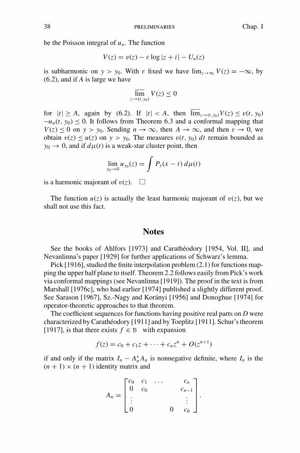
The coefficient sequences for functions having positive real parts on D werecharacterized by Caratheodory [1911] and by Toeplitz [1911]. Schur’s theorem[1917], is that there exists f ∈ B with expansion
f (z) = c0 + c1z + · · · + cnzn + O(zn+1)
if and only if the matrix In − A∗n An is nonnegative definite, where In is the
(n + 1) × (n + 1) identity matrix and
An =
⎡
⎢⎢⎣
c0 c1 . . . cn
0 c0 cn−1
......
0 0 c0
⎤
⎥⎥⎦ .

exercises and further results 39
A proof is outlined in Exercise 21 of Chapter IV. See Tsuji [1959], for a deriva-tion of Schur’s theorem from the Caratheodory-Toeplitz result. Pick’s theoremand Schur’s theorem are both contained in a recent result by Cantor [1981]who found the matrix condition necessary and sufficient for interpolation byfinitely many derivatives of a function in B at finitely many points in D.
The maximal function was introduced by Hardy and Littlewood [1930], butits importance was not widely recognized until much later. In their proof Hardyand Littlewood used rearrangements of functions. Lemma 4.4 is from Garsia’sbook [1970], where it is credited to W. H. Young. Also see Stein [1970] foranother covering lemma, which is valid in �n , and for a more general discussionof maximal functions and approximate identities.
The books by Zygmund [1968] and by Stein and Weiss [1971] contain moreinformation on the Marcinkiewicz theorem and other theorems on interpolationof operators.
Fatou’s theorem is from his classic paper [1906], which was written not longafter the introduction of the Lebesgue integral. Theorem 5.6 is from Carleson[1958, 1962a]. This proof of Lemma 5.5 is due to E. M. Stein.
We have barely touched the vast theory of subharmonic functions. Amongthe numerous important references we mention Tsuji [1959] and Hayman andKennedy [1976] as guides to the literature.
Some authors call the inequality
log | f (0)| ≤ 1
2π
∫log | f (eiθ )| dθ
and its relatives Jensen’s inequality, but we reserve the name for the inequalityof Lemma 6.1. Because the logarithm is concave, the two candidates for thename “Jensen’s inequality” actually go in opposite directions.
Exercises and Further Results
1. Let f (z) ∈ B satisfy f (0) = 0, | f ′(0)| = δ > 0. If |z| < η < δ, then
| f (z)| ≥(
δ − η
1 + ηδ
)
|z|,
and in the disc {|z| < η}, f (z) takes on each value w,
|w| <
(δ − η
1 − ηδ
)
η
exactly one time. (Hint: If g(z) = f (z)/z, then ρ(g(z), f ′(0)) ≤ |z|.)2. Suppose f (z) ∈ B .
(a) If f (z) has two distinct fixed points in D, then f (z) = z.(b) Let ε > 0, and suppose ρ( f (z1), z1) < ε, and ρ( f (z2), z2) < ε for z1
and z2 distinct points of D. If z lies on the hyperbolic geodesic arc joining z1

40 preliminaries Chap. I
to z2, then
ρ( f (z), z) ≤ Cε1/2
with C an absolute constant. (Hint: We can assume that z = 0, z1 = −r <
0, z2 = s > 0, and that f (z1) = z1. Then f (0) ∈ K (z1, r ) ∩ K (z2, s + ε) andthe euclidean description of the discs K (z1, r ) and K (z2, s + ε) yield an upperbound for | f (0)| = ρ( f (0), 0).)
(c) Let eiθ and eiϕ be distinct points of ∂D. Suppose {zn} and {wn} aresequences in D such that zn → eiθ , wn → eiϕ and such that ρ( f (zn), zn) →0, ρ( f (wn), wn) → 0. Then f fixes each point of the geodesic from eiθ to eiϕ ,and hence f (z) = z.
This result will reappear in Chapter X, Exercise 9.
3. Let I = (θ1, θ2) be an arc on the unit circle ∂D. Then
ω(z) =∫ θ2
θ1
Pz(θ ) dθ/2π, z ∈ D,
is the harmonic measure of I. Show
ω(z) = α/π − (θ2 − θ1)/2π,
where α = arg((eiθ2 − z)/(eiθ1 − z)), as shown in Figure I.6 (see Caratheodory[1954] or Nevanlinna [1953]).
Figure I.6.
4. For z, w ∈ D define the Gleason distance as
d(z, w) = sup{| f (z) − f (w)| : f ∈ B }and define the Harnack distance as
H (z, w) = sup log
{u(z)
u(w): u harmonic on D, u > 0
}
.
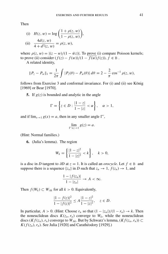
exercises and further results 41
Then
(i) H (z, w) = log
(1 + ρ(z, w)
1 − ρ(z, w)
)
,
(ii)4d(z, w)
4 + d2(z, w)= ρ(z, w),
where ρ(z, w) = |(z − w)/(1 − wz)|. To prove (i) compare Poisson kernels;to prove (ii) consider ( f (z) − f (w))/(1 − f (w) f (z)), f ∈ B .
A related identity,
‖Pz − Pw‖1 = 1
2π
∫|Pz(θ ) − Pw(θ )| dθ = 2 − 2
πcos−1 ρ(z, w),
follows from Exercise 3 and conformal invariance. For (i) and (ii) see Konig[1969] or Bear [1970].
5. If g(z) is bounded and analytic in the angle
� ={
z ∈ D :|1 − z|1 − |z| < α
}
, α > 1,
and if limx→1 g(x) = a, then in any smaller angle �′,
lim�′�z→1
g(z) = a.
(Hint: Normal families.)
6. (Julia’s lemma). The region
Wk ={ |1 − z|2
1 − |z|2 < k
}
, k > 0,
is a disc in D tangent to ∂D at z = 1. It is called an orocycle. Let f ∈ B andsuppose there is a sequence {zn} in D such that zn → 1, f (zn) → 1, and
1 − | f (zn)|1 − |zn| → A < ∞.
Then f (Wk) ⊂ WAk for all k > 0. Equivalently,
|1 − f (z)|21 − | f (z)|2 ≤ A
|1 − z|21 − |z|2 , z ∈ D.
In particular, A > 0. (Hint: Choose rn so that (1 − |zn|)/(1 − rn) → k. Thenthe noneuclidean discs K (zn, rn) converge to Wk , while the noneuclideandiscs (K f (zn), rn) converge to WAk . But by Schwarz’s lemma, (K f (zn, rn)) ⊂K ( f (zn), rn). See Julia [1920] and Caratheodory [1929].)
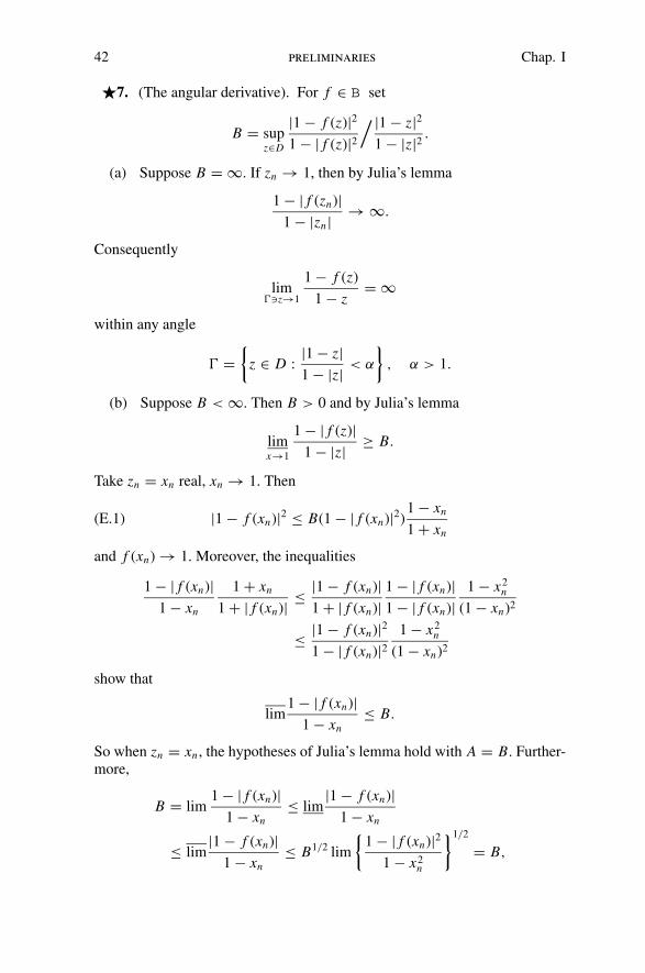
42 preliminaries Chap. I
�7. (The angular derivative). For f ∈ B set
B = supz∈D
|1 − f (z)|21 − | f (z)|2
/ |1 − z|21 − |z|2 .
(a) Suppose B = ∞. If zn → 1, then by Julia’s lemma
1 − | f (zn)|1 − |zn| → ∞.
Consequently
lim��z→1
1 − f (z)
1 − z= ∞
within any angle
� ={
z ∈ D :|1 − z|1 − |z| < α
}
, α > 1.
(b) Suppose B < ∞. Then B > 0 and by Julia’s lemma
limx→1
1 − | f (z)|1 − |z| ≥ B.
Take zn = xn real, xn → 1. Then
|1 − f (xn)|2 ≤ B(1 − | f (xn)|2)1 − xn
1 + xn(E.1)
and f (xn) → 1. Moreover, the inequalities
1 − | f (xn)|1 − xn
1 + xn
1 + | f (xn)| ≤ |1 − f (xn)|1 + | f (xn)|
1 − | f (xn)|1 − | f (xn)|
1 − x2n
(1 − xn)2
≤ |1 − f (xn)|21 − | f (xn)|2
1 − x2n
(1 − xn)2
show that
lim1 − | f (xn)|
1 − xn≤ B.
So when zn = xn , the hypotheses of Julia’s lemma hold with A = B. Further-more,
B = lim1 − | f (xn)|
1 − xn≤ lim
|1 − f (xn)|1 − xn
≤ lim|1 − f (xn)|
1 − xn≤ B1/2 lim
{1 − | f (xn)|2
1 − x2n
}1/2
= B,
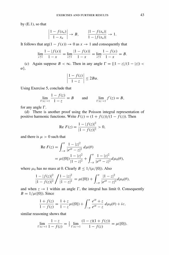
exercises and further results 43
by (E.1), so that∣∣∣∣1 − f (xn)
1 − xn
∣∣∣∣ → B,
|1 − f (xn)|1 − | f (xn)| → 1.
It follows that arg(1 − f (x)) → 0 as x → 1 and consequently that
limx↑1
1 − | f (x)|1 − x
= limx↑1
|1 − f (x)|1 − x
= limx↑1
1 − f (x)
1 − x= B.
(c) Again suppose B < ∞. Then in any angle � = {|1 − z|/(1 − |z|) <
α},∣∣∣∣1 − f (z)
1 − z
∣∣∣∣ ≤ 2Bα.
Using Exercise 5, conclude that
lim��z→1
1 − f (z)
1 − z= B and lim
��z→1f ′(z) = B,
for any angle �.(d) There is another proof using the Poisson integral representation of
positive harmonic functions. Write F(z) = (1 + f (z))/(1 − f (z)). Then
Re F(z) = 1 − | f (z)|2|1 − f (z)|2 > 0,
and there is μ > 0 such that
Re F(z) =∫ π
−π
1 − |z|2|eiθ − z|2 dμ(θ )
= μ({0})1 − |z|2|1 − z|2 +
∫ π
−π
1 − |z|2|eiθ − z|2 dμ0(θ ),
where μ0 has no mass at 0. Clearly B ≤ 1/(μ/{0}). Also
1 − | f (z)|2|1 − f (z)|2
/1 − |z|2|1 − z|2 = μ({0}) +
∫ π
−π
|1 − z|2|eiθ − z|2 dμ0(θ ),
and when z → 1 within an angle �, the integral has limit 0. ConsequentlyB = 1/μ({0}). Since
1 + f (z)
1 − f (z)= 1 + z
1 − zμ({0}) +
∫ π
−π
eiθ + z
eiθ − zdμ0(θ ) + ic,
similar reasoning shows that
lim��z→1
1 − z
1 − f (z)= 1
2lim
��z→1
(1 − z)(1 + f (z))
1 − f (z)= μ({0}).
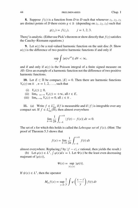
44 preliminaries Chap. I
8. Suppose f (z) is a function from D to D such that whenever z1, z2, z3
are distinct points of D there exists g ∈ B (depending on z1, z2, z3) such that
g(z j ) = f (z j ), j = 1, 2, 3.
Then f is analytic. (Either use Pick’s theorem or show directly that f (z) satisfiesthe Cauchy–Riemann equations.)
9. Let u(z) be a real-valued harmonic function on the unit disc D. Showu(z) is the difference of two positive harmonic functions if and only if
supr
∫|u(reiθ )| dθ < ∞,
and if and only if u(z) is the Poisson integral of a finite signed measure on∂D. Give an example of a harmonic function not the difference of two positiveharmonic functions.
10. Let E ⊂ � be compact, |E | = 0. Then there are harmonic functionsVn(z) on H , n = 1, 2, . . . , such that
(i) Vn(z) ≥ 0,(ii) limH �z→t Vn(z) = +∞, all t ∈ E ,
(iii) limn→∞ Vn(z) = 0, all z ∈ H .
11. (a) Write f ∈ L1loc if f is measurable and if | f | is integrable over any
compact set. If f ∈ L1loc(�), then almost everywhere
limh→0
1
2h
∫ x+h
x−h| f (t) − f (x)| dt = 0.
The set of x for which this holds is called the Lebesgue set of f (x). (Hint: Theproof of Theorem 5.3 shows that
f (x) = limh→0
1
2h
∫ x+h
x−hf (t) dt
almost everywhere. Replacing f by | f − c|, c rational, then yields the result.)(b) Let ϕ(x) ∈ L1,
∫ϕ(x)dx = 1. Let �(x) be the least even decreasing
majorant of |ϕ(x)|,�(x) = sup
|t |≥|x ||ϕ(t)|.
If ψ(x) ∈ L1, then the operator
Mϕ f (x) = supy>0
1
y
∫ϕ
(x − t
y
)
f (t) dt

exercises and further results 45
is weak-type 1–1,
|{x : Mϕ f (x) > λ}| ≤ C
λ‖ f ‖|1,
and Mϕ is bounded on L p, 1 < P ≤ ∞,
‖Mϕ f ‖p ≤ C p‖ f ‖p, 1 < p ≤ ∞.
If f ∈ L p, 1 ≤ p ≤ ∞, then
f (x) = limy→0
1
y
∫ϕ
(x − t
y
)
f (t) dt(E.2)
almost everywhere. More precisely, (E.2) holds at every point of the Lebesgueset of f , which is independent of ϕ.
(c) Formulate and prove a similar result about nontangential convergenceand nontangential maximal functions.
12. If f (x) has support a bounded interval I, then∫
I M f dx < ∞ if and
only if∫
I | f | log+ | f | dx < ∞ (Stein [1969]).
13. Let μ be a positive Borel measure on �, finite on compact sets, anddefine
Mμ f (x) = supI�x
1
μ(I )
∫
I| f | dμ.
Show
μ({Mμ f (x) > λ}) ≤ C
λ| f | dμ
and∫
|Mμ f |pdμ ≤ C p
∫| f |pdμ, 1 < p < ∞.
Conclude that for μ-almost all x,
limh→0
1
μ(x − h, x + h)
∫ x+h
x−h| f (t) − f (x)| dμ(t) = 0, f ∈ L1(μ).
14. If μ is a positive singular measure on �, then almost everywhere withrespect to μ,
limh→0
μ((x − h, x + h))
2h= ∞.
15. Let v(z) be a positive subharmonic function on the unit disc and define
m(r ) = 1
2π
∫v(reiθ ) dθ.

46 preliminaries Chap. I
Then m(r ) is an increasing convex function of log r. That is, if log r = t log r1 +(1 − t) log r2, 0 < t < 1, then
m(r ) ≤ t m(r1) + (1 − t) m(r2).
16. If ϕ(z) is of class C2 on a neighborhood of the closed disc �(z0, R) ={z : |z − z0| ≤ R}, then
ϕ(z0)= 1
2π
∫ 2π
0
ϕ(z0+Reiθ ) dθ− 1
2π
∫ ∫
�(z0,R)
log
∣∣∣∣
R
z − z0
∣∣∣∣ �ϕ(z) dx dy
by Green’s theorem.
�17. Let v(z) �= −∞ be upper semicontinuous on a plane domain �.(a) If v ∈ C2 and if �v = ∂ 2v/∂x2 + ∂ 2v/∂y2 ≥ 0, then v is subharmonic
on �. (Use Exercise 16.)(b) Let χ (z) ∈ C∞(�2) satisfy
χ ≥ 0, χ (z) = 0, |z| > 1,
∫χ (z)dx dy = 1.
Assume χ is radial, χ (z) = χ (|z|). Set χε(z) = ε−2χ (z/ε). Then
v ∗ χε(z) =∫
v(w)χε(z − w)dx dy
is C∞ on �ε = {z ∈ �: dist (z, ∂�) > ε} Prove v is subharmonic if and onlyif
�(v ∗ χε) ≥ 0
on �ε, for all ε > 0. In that case v ∗ χε decreases to v(z) everywhere on �.(c) Let C∞
0 (�) denote the space of infinitely differentiable functions havingcompact support contained in �. If ϕ ∈ C∞
0 (�) and f ∈ C2(�), then
∫∫
�
f �ϕ dx dy =∫∫
�
ϕ � f dx dy
(Green’s theorem again). If
∫∫
�
f � ϕ dx dy ≥ 0
when ϕ ≥ 0, ϕ ∈ C∞0 (�), then f is subharmonic on � (take ϕ(z) =
χε(z0 − z)). The weak Laplacian of v ∈ L1loc(�) is the functional
C∞0 (�) � ϕ →
∫∫
�
v�ϕ dx dy.
exercises and further results 47
If v is upper semicontinuous and if its weak Laplacian is nonnegative, that is,if
∫ ∫
�
v�ϕ dx dy ≥ 0
whenever ϕ ≥ 0, ϕ ∈ C∞0 (�), then v ∗ χε is subharmonic for every ε > 0, so
that v is subharmonic. Therefore v(z) is subharmonic if and only if its weakLaplacian is nonnegative.
(d) The weak Laplacian of log |z − z0|, z0 ∈ �, is a familiar measure. Findthe measure.
(e) If v(z) is subharmonic on �, then by the Riesz representation theorem,the weak Laplacian is a positive Borel measure finite on compact subsets of�. Denote this measure by �v. Then on �ε
v(z) = −1
2π
∫
�ε
log1
|z − w|d�v(w) + hε(z)
where hε is harmonic on �ε. This is called the Riesz decomposition of thesubharmonic function v(z). (see F. Riesz [1926]).

II
H p Spaces
The classical theory of the Hardy spaces H p is a mixture of real and com-plex analysis. This chapter is a short introduction to this theory, with specialemphasis put on the results and techniques we will need later.
The theory has three cornerstones:
(i) nontangential maximal functions;(ii) the subharmonicity of | f |p and log | f | for an analytic function f (z);
(iii) the use of Blaschke products to reduce problems to the case of a non-vanishing analytic function.
There are two H p theories, one for the disc and another for the upper halfplane. We introduce these twin theories simultaneously.
1. Definitions
Let 0 < p < ∞ and let f (z) be an analytic function on D. We say f ∈H p = H p(D) if
supr
1
2π
∫| f (reiθ )|p dθ = ‖ f ‖p
H p < ∞.
If p = ∞, we say f ∈ H∞ if f (z) is a bounded analytic function on D andwe write
‖ f ‖∞ = supz∈D
| f (z)|.
Thus the unit ball of H∞, { f ∈ H∞ : ‖ f ‖∞ ≤ 1} is the class B considered inthe first two sections of Chapter I. The remarks on subharmonic functions inChapter I show that f (z) ∈ H p if and only if the subharmonic function | f (z)|p
has a harmonic majorant, and that for p < ∞, ‖ f ‖pH p is the value of the least
harmonic majorant at z = 0. This second definition of H p in terms of harmonicmajorants is conformally invariant. It is used to define H p functions on anyplane domain or Riemann surface.
48
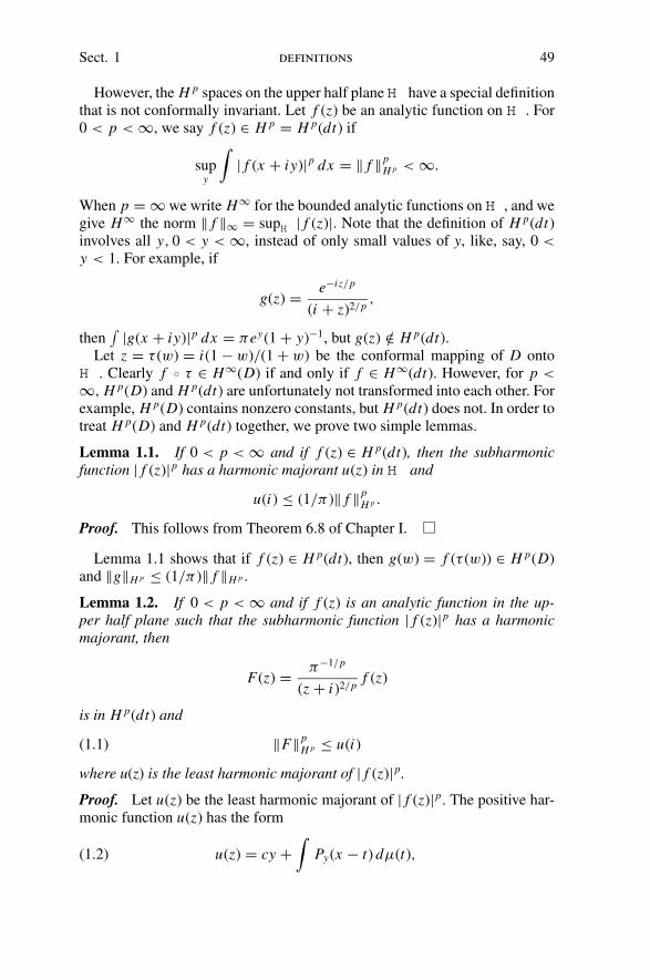
Sect. 1 definitions 49
However, the H p spaces on the upper half plane H have a special definitionthat is not conformally invariant. Let f (z) be an analytic function on H . For0 < p < ∞, we say f (z) ∈ H p = H p(dt) if
supy
∫| f (x + iy)|p dx = ‖ f ‖p
H p < ∞.
When p = ∞ we write H∞ for the bounded analytic functions on H , and wegive H∞ the norm ‖ f ‖∞ = supH | f (z)|. Note that the definition of H p(dt)involves all y, 0 < y < ∞, instead of only small values of y, like, say, 0 <
y < 1. For example, if
g(z) = e−i z/p
(i + z)2/p,
then∫ |g(x + iy)|p dx = πey(1 + y)−1, but g(z) /∈ H p(dt).
Let z = τ (w) = i(1 − w)/(1 + w) be the conformal mapping of D ontoH . Clearly f ◦ τ ∈ H∞(D) if and only if f ∈ H∞(dt). However, for p <
∞, H p(D) and H p(dt) are unfortunately not transformed into each other. Forexample, H p(D) contains nonzero constants, but H p(dt) does not. In order totreat H p(D) and H p(dt) together, we prove two simple lemmas.
Lemma 1.1. If 0 < p < ∞ and if f (z) ∈ H p(dt), then the subharmonicfunction | f (z)|p has a harmonic majorant u(z) in H and
u(i) ≤ (1/π )‖ f ‖pH p .
Proof. This follows from Theorem 6.8 of Chapter I.
Lemma 1.1 shows that if f (z) ∈ H p(dt), then g(w) = f (τ (w)) ∈ H p(D)and ‖g‖H p ≤ (1/π )‖ f ‖H p .
Lemma 1.2. If 0 < p < ∞ and if f (z) is an analytic function in the up-per half plane such that the subharmonic function | f (z)|p has a harmonicmajorant, then
F(z) = π−1/p
(z + i)2/pf (z)
is in H p(dt) and
‖F‖pH p ≤ u(i)(1.1)
where u(z) is the least harmonic majorant of | f (z)|p.
Proof. Let u(z) be the least harmonic majorant of | f (z)|p. The positive har-monic function u(z) has the form
u(z) = cy +∫
Py(x − t) dμ(t),(1.2)

50 Hpspaces Chap. II
where c ≥ 0 and where μ is a positive measure on � such that∫
(1 + t2)−1 dμ(t) < ∞.
Consequently,
|F(z)|p = 1
π (x2 + (1 + y)2)| f (z)|p,
so that by (1.2) and Fubini’s theorem,∫
|F(x + iy)|pdx ≤ c + 1
π
∫1
1 + x2
∫Py(x − t) dμ(t)dx
= c +∫
Py(t)∫
P1(x − t)dμ(x)dt = c + (u(i) − c),
Therefore, F(z) ∈ H p(dt). The proof of Theorem I.6.8 shows that∫
|F(x + iy)|pdx
is a decreasing function of y. Hence,
‖F‖pH p = lim
y→0
∫|F(x + iy)|pdx
and
‖F‖pH p = −c + lim
y→0u((1 + y)i) = 1
π
∫dμ(t)
1 + t2≤ u(i).
Lemma 1.2 shows that if g(w) ∈ H p(D), then
F(z) = π−1/p
(z + i)2/pg(w(z)) ∈ H p(dt),
where w(z) = τ−1(z), and ‖F‖H p ≤ ‖g‖H p . We shall see in Section 3 that theconverse of Lemma 1.2 is true and that ‖F‖H p = ‖g‖H p . Notice that because(z + i)−2/p has no zeros on H , the family of zero sets of H p functions isinvariant under z = τ (w).
For p ≥ 1, H p is a normed linear space. For p < 1, the inequality
|z1 + z2|p ≤ |z1|p + |z2|p
shows that H p is a metric space with metric
d( f, g) = ‖ f − g‖pH p .
Theorem 1.3. For 0 < p ≤ ∞, H p is complete.

Sect. 2 blaschke products 51
Proof. We can assume p < ∞. We give the proof in the upper half plane; thereasoning for the disc is very similar. The key inequality
| f (x + iy)| ≤ (2/πy)1/p‖ f ‖H p , y > 0,(1.3)
follows from (6.2) of Chapter I. It shows that any H p Cauchy sequence { fn}converges pointwise on H to an analytic function f (z). Fatou’s lemma thenshows∫
| f (x + iy) − fn(x + iy)|pdx ≤ limm→∞
∫| fm(x + iy) − fn(x + iy)|pdx
≤ limm→∞
‖ fm − fn‖pH p .
Hence ‖ f − fn‖pH p ≤ limm→∞‖ fm − fn‖p
H p , and H p is complete.
2. Blaschke Products
We show that the zeros {zn} of a nonzero H p function on the disc satisfyBlaschke’s condition
∑(1 − |zn|) < ∞.(2.1)
It is noteworthy that (2.1) does not depend on p. When (2.1) holds, specialH∞ functions called Blaschke products will be constructed to have {zn} aszeros. Blaschke products will play an expanding role in the later chapters ofthis book.
Theorem 2.1. Let f (z) be an analytic function on the disc, f ≡ 0, and let{zn} be the zeros of f (z). If log | f (z)| has a harmonic majorant, then
∑(1 − |zn|) < ∞.
If f (0) = 0 and if u(z) is the least harmonic majorant of log | f (z)|, then∑
(1 − |zn|) ≤ u(0) − log | f (0)|.Proof. Replacing f (z) by f (z)/zN if necessary, we can assume f (0) = 0.Then by Theorem I.6.7,
supr
∫log | f (reiθ )|dθ/2π = u(0),
where u is the least harmonic majorant of log | f (z)|. Fix r < 1 so that |zn| =r for all n, and let z1, . . . , zn be those zeros with |z j | < r . Then f (r z) isanalytic on the closed disc and f (r z) has zeros z1/r , z2/r , . . . , zn/r . Let Br (z) =�n
j=1(z − z j/r )/(1 − z j z/r ), a finite Blaschke product with the same zeros as
f (r z), and let g(z) = f (r z)/Br (z). Then g is analytic and zero free on D,

52 Hpspaces Chap. II
so that
log |g(0)| = 1
2π
∫log |g(eiθ )|dθ.
Since |g(eiθ )| = | f (reiθ )|, this gives the familiar Jensen formula
log | f (0)| +∑
|z j |<r
logr
|z j | = 1
2π
∫log | f (reiθ )|dθ.
Letting r tend to 1 then yields
∑log
1
|z j | = limr→1
1
2π
∫log | f (reiθ )|dθ − log | f (0)| = u(0) − log | f (0)|.
Since 1 − |z j | ≤ log(1/|z j |), the theorem is proved.
If f ∈ H p(D), then log | f | ≤ (1/p)| f |p, and log | f | has a harmonic ma-jorant. Hence, if f ∈ H p(D), or by Lemma 1.1 if f (w) = F(z(w)) whereF ∈ H p(dt), then
∑(1 − |zn|) < ∞.
Theorem 2.2. Let {zn} be a sequence of points in D such that∑
(1 − |zn|) < ∞.
Let m be the number of zn equal to 0. Then the Blaschke product
B(z) = zm∏
|zn |=0
−zn
|zn|z − zn
1 − znz(2.2)
converges on D. The function B(z) is in H∞(D) and the zeros of B(z) areprecisely the points zn, each zero having multiplicity equal to the number oftimes it occurs in the sequence {zn}. Moreover |B(z)| ≤ 1 and
|B(eiθ )| = 1
almost everywhere.
By definition, a Blaschke product on D is a function of the form (2.2).
Proof. We can suppose |zn| > 0 for all n. Let
bn(z) = −zn
|zn|z − zn
1 − znz.
Then the product∏
bn converges on D to an analytic function having {zn} forzeros if and only if
∑ |1 − bn(z)| converges uniformly on each compact subsetof D. But by a calculation,
|1 − bn(z)| = |zn + z|zn|||zn||1 − znz| (1 − |zn|) ≤ 1 + |z|
1 − |z| (1 − |zn|)
and the convergence follows from (2.1).

Sect. 2 blaschke products 53
Since |bn(z)| ≤ 1, it is clear that B(z) ∈ H∞ and |B(z)| ≤ 1. The boundedharmonic function B(z) has nontangential limits |B(eiθ )| ≤ 1 almost every-where. To see that |B(eiθ )| = 1 almost everywhere, set Bn(z) = ∏n
1 bk(z). ThenB/Bn is another Blaschke product and
∣∣∣∣
B(0)
Bn(0)
∣∣∣∣ ≤ 1
2π
∫ |B(eiθ )||Bn(eiθ )|dθ = 1
2π
∫|B(eiθ )|dθ.
Letting n → ∞ now yields
1
2π
∫|B(eiθ )|dθ = 1.
so that |B(eiθ )| = 1 almost everywhere.
The purpose of the convergence factors −zn/|zn| is to make∑
arg bn(z)converge. To remember the convergence factors, note that they are chosen sothat bn(0) > 0.
By Theorem 2.1 and Theorem 2.2, the analytic function f (z) has a factor-ization
f (z) = B(z)g(z), z ∈ D,
where B(z) is a Blaschke product and where g(z) has no zeros on D, if andonly if the subharmonic function log | f (z)| has a harmonic majorant.
In the upper half plane condition (2.1) is replaced by
∑ yn
1 + |zn|2 < ∞, zn = xn + iyn,(2.3)
and the Blaschke product with zeros {zn} is
B(z) =(
z − i
z + i
)m ∏
zn =i
|z2n + 1|
z2n + 1
z − zn
z − zn.
If the moduli |zn| are bounded, (2.3) becomes∑
yn < ∞, and the convergencefactors are not needed because
∏((z − zn)/(z − zn)) already converges.
Theorem 2.3 (F. Riesz). Let 0 < p < ∞. Let f (z) ∈ H p(D), f ≡ 0, let {zn}be the zeros of f (z), and let B(z) be the Blaschke product with zeros {zn}. Theng(z) = f (z)/B(z) is in H p(D) and
‖g‖H p = ‖ f ‖H p .
Proof. It was noted above that B(z) converges when f ∈ H p. Let Bn bethe finite Blaschke product with zeros z1, z2, . . . , zn , and let gn = f/Bn . Fixr < 1. Then by Theorem I.6.6,
∫|gn(reiθ )|p dθ
2π≤ lim
R→1
∫ | f (Reiθ )|p
|Bn(Reiθ )|p
dθ
2π.

54 Hpspaces Chap. II
If 1 − R is small, then |Bn(Reiθ )| > 1 − ε, so that
∫|gn(reiθ )|p dθ
2π≤ lim
R→1
∫| f (Reiθ )|p dθ
2π= ‖ f ‖p
H p .
Since |gn| increases to |g|, and since |g| ≥ | f |, this gives‖g‖pH p = ‖F‖p
H p .
Theorem 2.3 is also true for H p(dt), because the proof of Theorem I.6.8shows that
supy
∫| f (x + iy)|pdx = lim
y→0
∫| f (x + iy)|pdx .
Blaschke products have a simple characterization in terms of harmonic ma-jorants.
Theorem 2.4. Let f (z) ∈ H∞(D)‖ f ‖∞ ≤ 1. Then the following are equiv-alent.
(a) f (z) = λB(z), where λ is constant, |λ| = 1, and B(z) is a Blaschkeproduct.
(b) limr→1
∫log | f (reiθ )|dθ/2π = 0.
(c) The least harmonic majorant of log | f (z)|is 0.
Proof. Theorem I.6.7 shows that (b) and (c) are equivalent.Suppose f (z) is the Blaschke product with zeros {zn}, and let ε > 0. We may
divide f (z) by a finite Blaschke product Bn(z) so that |( f/Bn)(0)| > 1 − ε.Since Bn is continuous on D and |Bn(eiθ )| = 1,
limr→1
∫log | f (reiθ )|dθ = lim
r→1
∫log
∣∣∣∣
f
Bn(reiθ )
∣∣∣∣ dθ.
But since log | f/Bn| is subharmonic and negative,
log(1 − ε) ≤∫
log
∣∣∣∣
f
Bn(reiθ )
∣∣∣∣
dθ
2π≤ 0.
Therefore (b) holds.Suppose (c) holds. Let g(z) = f (z)/B(z), where B(z) is the Blaschke prod-
uct formed from the zeros of f (z). Then
log | f (z)| ≤ log |g(z)| ≤ 0
because ‖ f ‖∞ ≤ 1. Since log |g(z)| is a harmonic majorant of log | f (z)|, (c)implies that log |g(z)| = 0. Hence g(z) = λ, where λ is a constant and |λ| = 1,and so (a) holds.

Sect. 3 maximal functions and boundary values 55
3. Maximal Functions and Boundary Values
Let f (z) ∈ H p(dt). If p > 1, we know from Chapter I that the nontangentialmaximal function f ∗(t) is in L p, and that f (z) converges nontangentially to anL p function f (t) almost everywhere. An important feature of the H p spacesis that these results remain true for all p, 0 < p ≤ ∞.
Theorem 3.1. Let 0 < p < ∞ and let f (z) be a function in H p(dt). Thenfor any α > 0, the nontangential maximal function
f ∗(t) = supz∈α(t)
| f (z)|
is in L p(�) and
‖ f ∗‖pp ≤ Aα‖ f ‖p
H p ,(3.1)
where the constant Aα depends only on α. Moreover, for almost all t ∈ �, f (z)has a nontangential limit f (t) ∈ L p(�) satisfying
∫| f (t)|pdt = ‖ f ‖p
p = ‖ f ‖pH p(3.2)
and
limy→0
‖ f (t + iy) − f (t)‖pp = 0.(3.3)
Proof. Except for the fact that the constant Aα in (3.1) does not depend on p,the case p > 1 of the theorem is proved in Section 5 of Chapter I. To stretch pbelow 1 we use Theorem 2.3 above. Suppose f ∈ H p, f ≡ 0. Let B(z) be theBlaschke product formed from the zeros of f (z) and let g(z) = f (z)/B(z).Then ‖g‖H p = ‖ f ‖H p , and since | f (z)| ≤ |g(z)|, | f ∗(t)| ≤ |g∗(t)|. Let p1 >
1. Since g has no zeros and g ∈ H p, the analytic function g p/p1 is in H p1 .Consequently (g∗)p/p1 = (g p/p1 )∗ is in L p1 , and hence by Theorem I.5.1,
‖g∗‖pp = ‖(g p/p1 )∗‖p1
p1≤ Bp1
‖g‖pH p .
Taking p1 = 2 we see that (3.1) holds with a constant independent of p, becausef ∗ ≤ g∗.
Now G(z) = (g(z))p/p1 has a nontangential limit G(t) almost everywhere.Taking p1/p to be a positive integer m, we see that g(z) = G(z)m also hasnon-tangential limits. Since B(z) has boundary values almost everywhere weconclude that f (z) has a nontangential limit almost everywhere. It now followsfrom (3.1) and the dominated convergence theorem that f (t) ∈ L p(�) and that(3.2) and (3.3) hold.
The equality (3.2) establishes an isometry between H p(dt) and a closedsubspace of L p(�). For p < 1, although L p is not a Banach space, it is, like H p,a complete metric space under the metric d( f, g) = ‖ f − g‖p
p. When p ≥ 1,this space of boundary values of H p functions has a simple characterization.
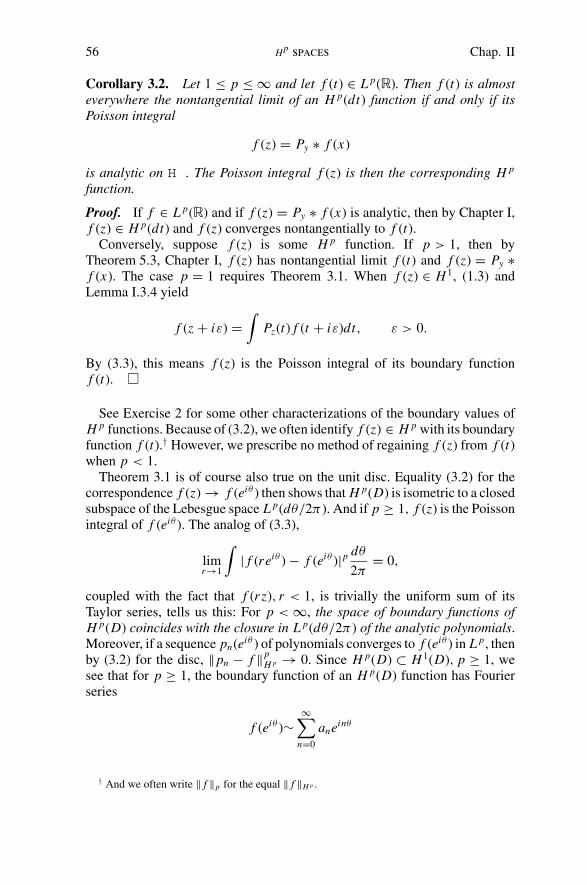
56 Hpspaces Chap. II
Corollary 3.2. Let 1 ≤ p ≤ ∞ and let f (t) ∈ L p(�). Then f (t) is almosteverywhere the nontangential limit of an H p(dt) function if and only if itsPoisson integral
f (z) = Py ∗ f (x)
is analytic on H . The Poisson integral f (z) is then the corresponding H p
function.
Proof. If f ∈ L p(�) and if f (z) = Py ∗ f (x) is analytic, then by Chapter I,f (z) ∈ H p(dt) and f (z) converges nontangentially to f (t).
Conversely, suppose f (z) is some H p function. If p > 1, then byTheorem 5.3, Chapter I, f (z) has nontangential limit f (t) and f (z) = Py ∗f (x). The case p = 1 requires Theorem 3.1. When f (z) ∈ H 1, (1.3) andLemma I.3.4 yield
f (z + iε) =∫
Pz(t) f (t + iε)dt, ε > 0.
By (3.3), this means f (z) is the Poisson integral of its boundary functionf (t).
See Exercise 2 for some other characterizations of the boundary values ofH p functions. Because of (3.2), we often identify f (z) ∈ H p with its boundaryfunction f (t).† However, we prescribe no method of regaining f (z) from f (t)when p < 1.
Theorem 3.1 is of course also true on the unit disc. Equality (3.2) for thecorrespondence f (z) → f (eiθ ) then shows that H p(D) is isometric to a closedsubspace of the Lebesgue space L p(dθ/2π ). And if p ≥ 1, f (z) is the Poissonintegral of f (eiθ ). The analog of (3.3),
limr→1
∫| f (reiθ ) − f (eiθ )|p dθ
2π= 0,
coupled with the fact that f (r z), r < 1, is trivially the uniform sum of itsTaylor series, tells us this: For p < ∞, the space of boundary functions ofH p(D) coincides with the closure in L p(dθ/2π ) of the analytic polynomials.Moreover, if a sequence pn(eiθ ) of polynomials converges to f (eiθ ) in L p, thenby (3.2) for the disc, ‖pn − f ‖p
H p → 0. Since H p(D) ⊂ H 1(D), p ≥ 1, wesee that for p ≥ 1, the boundary function of an H p(D) function has Fourierseries
f (eiθ )∼∞∑
n=0
aneinθ
† And we often write ‖ f ‖p for the equal ‖ f ‖H p .

Sect. 3 maximal functions and boundary values 57
supported on the nonnegative integers, and its Fourier coefficients
an = 1
2π
∫f (eiθ )e−inθdθ = lim
r→1
1
2π i
∫
|z|=r
f (z)dz
zn+1
are the Taylor coefficients of the H p function f (z) = ∑anzn . Thus H p theory
is a natural bridge between Fourier analysis and complex analysis.In the upper half plane we see from (3.3) that the uniformly continuous
functions in H∞ ∩ H p are dense in H p, because for f ∈ H p,
| f (x + iy)| ≤(
2
πy
)1/p
‖ f ‖H p , y > 0,
and
| f ′(x + iy)| ≤ 2
y
(4
πy
)1/p
‖ f ‖H p ,
by the preceding inequality and by Schwarz’s lemma, scaled to the disc(z, y/2). We will need some very smooth classes of analytic functions thatare dense in H p(dt) and that will play the role of the polynomials in the disccase. Let N be a positive integer, and let AN be the family of H∞(dt) functionssatisfying
(i) f (z) is continuous on H and f (t) is infinitely differentiable, f ∈ C∞.
(ii) lim|z|→∞ |z|N | f (z)| = 0, z ∈ H .
Corollary 3.3. Let N be a positive integer. For 0 < p < ∞, the class AN isdense in H p(dt). For f (z) ∈ H∞, there are functions fn(z) in AN such that‖ fn‖∞ ≤ ‖ f ‖∞ and such that | fn(t)| ≤ | f (t)| almost everywhere.
Proof. Were it not for the decay condition (ii), we could approximate f by thesmooth functions f (z + i/n), which converge in H p norm to f (t) if p < ∞and which converge boundedly pointwise almost everywhere to f (t) if p = ∞.Now there are some special functions gk(z) such that
(a) gk(z) ∈ AN ,(b) |gk(z)| ≤ 1, z ∈ H ,(c) gk(z) → 1, z ∈ H .
Before we construct the functions gk , we note that the functions
fn(z) = gn(z) f (z + i/n)
in AN then give the desired approximation.The heart of the proof, constructing the functions gk(z), will be done in
the unit disc, where w = −1 corresponds to z = ∞. Let αk < 1, αk → 1. Thefunction
hk(w) =(
w + αk
1 + αkw
)N+1
58 Hpspaces Chap. II
has an (N + 1)-fold zero at −αk . These hk(w) are bounded by 1, and with Nfixed they converge to 1 uniformly on compact subsets of D\{−1}. Then thefunctions
gk(z) = hk(αk, w), w = i − z
i + z,
satisfy (a)–(c).
Now we can clarify the relation between H p(D) and H p(dt).
Corollary 3.4. Let 0 < p < ∞, let f (z) be an analytic function in the upperhalf plane and let
F(z) = π−1/p
(z + i)2/pf (z).
Then | f (z)|p has a harmonic majorant if and only if F(z) ∈ H p. In that case
‖F‖pH p = u(i),(3.4)
where u(z) is the least harmonic majorant of | f (z)|p.
Proof. Let g(w) = f (z), z = i(1 − w)/(1 + w). The corollary asserts thatg ∈ H p(D) if and only if F ∈ H p(dt), and that ‖g‖p = ‖F‖p. If N > 2/pand if F ∈ AN , then the corresponding function g(w) is bounded on D and,because dθ/2π corresponds to dt/π (1 + t2),
∫|g(θ )|p dθ
2π=
∫|F(t)|pdt.
By the density of AN in H p, it follows from (3.2) that g ∈ H p(D) wheneverF ∈ H p(dt) and that
‖g‖Hp = ‖F‖Hp .
Since Lemma 1.2 shows F ∈ H p(dt) if g(w) ∈ H p(D), that concludes theproof.
Incidentally, the fact that we have the equality (3.4) instead of the inequality(1.1) means that in the formula (1.2) for the least harmonic majorant of | f (z)|p,the constant term is c = 0. We shall see in Section 4 that the least harmonicmajorant is the Poisson integral of the L1 function | f (t)|p.
The next corollary is noteworthy because of the recent discovery, for p ≤ 1,of its converse, which will be proved in Chapter III.
Corollary 3.5. Let 0 < p < ∞ and let u(z) be a real-valued harmonic func-tion on the upper half plane H . If u(z) is the real part of a function f (z) ∈ H p,then
u∗(t) = supα(t)
|u(z)|
is in L p(�).

Sect. 3 maximal functions and boundary values 59
The proof from Theorem 3.1 is trivial.Let us reexamine the boundary values in the case p = 1. If the harmonic
function u(z) satisfies
supy
∫|u(x + iy)|dx < ∞,
then u(z) need not be the Poisson integral of its nontangential limit u(t). All wecan say is that u(z) is the Poisson integral of a finite measure. However, if u(z)is also an analytic function, then the measure is absolutely continuous, and itsdensity is the boundary value u(t). The reason is that the maximal functionu∗(t) is integrable.
Theorem 3.6. If f (z) ∈ H 1(dt), then f (z) is the Poisson integral of its bound-ary values:
f (z) =∫
Py(x − t) f (t)dt.(3.5)
Conversely, if μ is a finite complex measure on � such that the Poisson integralf (z) = Py ∗ μ(x) is an analytic function onH , then μ is absolutely continuousand
dμ = f (t) = dt,
where f (t) is the boundary function of the Poisson integral f (z) of μ.
Proof. If f (z) ∈ H 1, then (3.5) was already obtained in the proof of Corol-lary 3.2. Conversely, if f (z) = Py, ∗μ(x) is an analytic function, then byMinkowski’s integral inequality it is an H 1 function and hence it is thePoisson integral of its boundary value f (t). The difference measure dv(t) =dμ(t) − f (t)dt has Poisson integral zero, and so v = 0 by Theorem I.3.1.
Lemma 3.7. Let f (z) ∈ H 1. Then the Fourier transform
f (s) =∫ ∞
−∞f (t)e−2π ist dt = 0
for all s ≤ 0.
Proof. By the continuity of f → f , we may suppose∫ ∈ AN . Then for
s ≤ 0, F(z) = f (z)e−2π isz is also inAN . The result now follows from Cauchy’stheorem because
∫ π
0
|F(Reiθ )|R dθ → 0 (R → ∞).
Notice that
Pz(t) = 1
2π i
(1
t − z− 1
t − z
)
.(3.6)

60 Hpspaces Chap. II
Also notice that for f ∈ H 1, Lemma 3.7 applied to (t − z)−1 f (t) yields
∫f (t)
t − zdt = 0, Im z > 0.
Theorem 3.8. Let dμ(t) be a finite complex measure on � such that either
∫dμ(t)
t − z= 0 on Im z < 0,(a)
or
μ(s) =∫
e−2π ist dμ(t) = 0 on s < 0.(b)
Then dμ is absolutely continuous and dμ = f (t) dt, where f (t) ∈ H 1.
Proof. If (a) holds, then by (3.6) f (z) = Py ∗ μ(x) is analytic and the resultfollows from Theorem 3.6.
Assume (b) holds. The Poisson kernel Py(t) has Fourier transform
∫e−2π ist Py(t) dt = e−2π |s|y,
because Py(−s) = Py(s) since Py is real, and because if s ≤ 0, e−2π isz is thebounded harmonic function with boundary values e−2π ist . Let fy(x) = Py ∗μ(x). By Fubini’s theorem, fy has Fourier transform
f y(s) ={
e−2πxyμ(s), s ≥ 0,
0, s < 0.
Since f y ∈ L1, Fourier inversion implies
fy(x) =∫
e2π i xs f y(s) ds =∫ ∞
0
e2π i(x+iy)sμ(s) ds.
Differentiating under the integral sign then shows that f (z) = fy(x) is analytic,and Theorem 3.6 now implies that f (z) ∈ H 1.
The disc version of Theorem 3.6, or equivalently Theorem 3.8, is one halfof the famous F. and M. Riesz theorem. The other half asserts that if f (z) ∈H 1, f ≡ 0, then | f (t)| > 0 almost everywhere. This is a consequence of astronger result proved in the next section.
The theorem on Carleson measures, Theorem I.5.6, also extends to the H p
spaces, 0 < p ≤ 1, because the key estimate in its proof was the maximaltheorem.

Sect. 4 (1/π)∫
(log | f (t)|/(1 + t2)) dt > − ∞ 61
Theorem 3.9 (Carleson). Let σ be a positive measure in the upper half plane.Then the following are equivalent:
(a) σ is a Carleson measure: for some constant N (σ ),
σ (Q) ≤ N (σ )h
for all squares
Q = {x0 < x < x0 + h, 0 < y < h}.(b) For 0 < p < ∞,
∫| f |pdσ ≤ A‖ f ‖p
H p , f ∈ H p.
(c) For some p, 0 < p < ∞, f ∈ L p(σ ) for all f ∈ H p.
Proof. That (a) implies (b) follows from (3.1) and Lemma I.5.5 just as in theproof of Theorem I.5.6.
Trivially, (b) implies (c). On the other hand, if (c) holds for some fixedp < ∞, then (b) holds for the same value p. This follows from the closed graphtheorem, which is valid here even when p < 1 (see Dunford and Schwartz[1958, p. 57]). One can also see directly that if there are { fn} in H p with‖ fn‖p = 1 but
∫ | fn|pdσ → ∞, then the sum �αn fn , when the αn , are chosenadroitly, will give an H p function for which (c) fails.
Now suppose (b) holds for some p > 0. Let Q be the square {x0 < x <
x0 + y0, 0 < y < y0} and let
f (z) =(
1
π
y0
(z − z0)2
)1/p
,
where z0 = x0 + iy0. Then f ∈ H p and ‖ f ‖pp = ∫
Pz0(t)dt = 1. Since
| f (z)|p ≥ (5πy0)−1, z ∈ Q, we have
σ (Q) ≤ σ ({z : | f (z)| > (5πy0)−1/p}) ≤ 5π Ay0,
so that (a) holds.
4. (1/π)∫
(log | f (t)|/(1 + t2)) dt > − ∞A fundamental result of H p theory is that the condition of this section’s
title characterizes the moduli of H p functions | f (t)| among the positive L p
functions. In the disc, this result is due to Szego for p = 2 and to F. Riesz forthe other p. For functions analytic across ∂D, the inequality (4.1) below wasfirst noticed by Jensen [1899] and for this reason the inequality is sometimescalled Jensen’s inequality. We prefer to use that name for the inequality aboutaverages and convex functions given in Theorem I.6.1.
In this section the important thing about an H p function will be the fact thatthe subharmonic function
log | f (reiθ )| ≤ (1/p)| f (reiθ )|p
62 Hpspaces Chap. II
is majorized by a positive L1 function of θ . It will be simpler to work at firston the disc.
Theorem 4.1. If 0 < p ≤ ∞ and if f (z) ∈ H p(D), f ≡ 0, then
1
2π
∫log | f (eiθ )|dθ > −∞.
If f (0) ≡ 0, then
log | f (0)| ≤ 1
2π
∫log | f (eiθ )|dθ,(4.1)
and more generally, if f (z0) ≡ 0
log | f (z0)| ≤ 1
2π
∫log | f (eiθ )|Pz0
(θ )dθ.(4.2)
Proof. By Theorem I.6.7 and by the subharmonicity of log | f |,
log | f (z)| ≤ limr→1
1
2π
∫log | f (reiθ )|Pz(θ )dθ.
Since log | f (reiθ )| → log | f (eiθ ) almost everywhere, and since these func-tions are bounded above by the integrable function (1/p)| f ∗(θ )|p, where f ∗is the maximal function, we have
∫log+ | f (reiθ )|Pz0
(θ ) dθ →∫
log+ | f (eiθ )|Pz0(θ ) dθ.
Fatou’s lemma can now be applied to the negative parts to give us
limr→1
1
2π
∫log | f (reiθ )|Pz0
(θ ) dθ ≤ 1
2π
∫log | f (eiθ )|Pz0
(θ ) dθ.
This proves (4.2) and (4.1). The remaining inequality follows by removing anyzero at the origin.
Note that the same result in the upper half plane
log | f (z0)| ≤∫
log | f (t)|Pz0(t)dt, f ∈ H p,(4.3)
follows from Theorem 4.1 and from Lemma 1.1 upon a change of variables.
Corollary 4.2. If f (z) ∈ H p and if f (t) = 0 on a set of positive measure,then f = 0.
Corollary 4.2 gives the other half of the F. and M. Riesz theorem. If dμ(t) isa finite measure such that py ∗ μ(x) is analytic, then not only is dμ absolutelycontinuous to dt, but also dt is absolutely continuous to dμ.
Corollary 4.3. Let 0 < p, r ≤ ∞. If f (z) ∈ H p and if the boundary functionf (t) ∈ Lr , then f (z) ∈ Hr .
Sect. 4 (1/π)∫
(log | f (t)|/(1 + t2)) dt > − ∞ 63
This corollary is often written
H p ∩ Lr ⊂ Hr .
Proof. Applying Jensen’s inequality, with the convex function ϕ(s) =exp(rs) and with the probability measure Py(x − t)dt , to (4.3) gives
| f (z)|r ≤∫
| f (t)|r Py(x − t) dt.
Integration in x then yields f ∈ Hr .
Theorem 4.4. Let h(t) be a nonzero nonnegative function in L p(�). Thenthere is f (z) ∈ H p(dt) such that | f (t)| = h(t) almost everywhere if and onlyif
∫log h(t)
1 + t2dt > − ∞.(4.4)
Proof. It has already been proved that (4.4) is a necessary condition. To show(4.4) is sufficient, note that since log h ≤ (1/p)|h|p, (4.4) holds if and only iflog h ∈ L1(dt/(1 + t2)). Let u(z) be the Poisson integral of log h(t) and let v(z)be any harmonic conjugate of u(z). (Since H is simply connected, there existsa harmonic conjugate function v(z) such that u + iv is analytic. The conjugatefunction v(z) is unique except for an additive constant.) The function we areafter is
f (z) = eu(z)+iv(z),
which is an analytic function on H . When p < ∞ Jensen’s inequality againgives
| f (z)|p ≤∫
Py(x − t)|h(t)|pdt
and therefore f ∈ H p. If p = ∞ then u is bounded above and so f ∈ H∞.
When p = ∞, (4.4) is especially important. Let h ≥ 0, h ∈ L∞, and sup-pose 1/h ∈ L∞. Then f = eu+iv ∈ H∞ and also
1/ f = e−(u+iv) ∈ H∞.
In other words, f is an invertible function in H∞. We write f ∈ (H∞)−1. Foremphasis, we state this fact separately, writing g = log h, so that g ∈ L∞ ifh ∈ L∞ and 1/h ∈ L∞.
Theorem 4.5. Every real-valued function g(t) in L∞ has the form log | f (t)|,where f ∈ (H∞)−1 is an invertible function in H∞.
In the language of uniform algebra theory, Theorem 4.5 asserts that H∞ isa strongly logmodular subalgebra of L∞. It is also a logmodular subalgebra

64 Hpspaces Chap. II
of L∞, which means that the set
log |(H∞)−1| = {log | f (t)| : f ∈ H∞, 1/ f ∈ H∞}is dense in L∞
� , the space of real L∞ functions. The Banach algebra aspectsof H∞ will be discussed in some detail later; for the present we only want tosay that Theorem 4.4 is a powerful tool for constructing H p functions.
Let h(t) ≥ 0 satisfy∫ | log h(t)|dt
1 + t2< ∞.
The function
f (z) = eu(z)+iv(z),
where
u(z) = Py ∗ (log h)(x)(4.5)
and where v(z) is a harmonic conjugate function of u(z), is called an outerfunction. The outer function f (z) is determined by h(t) except for the uni-modular constant factor arising from the choice of the conjugate function v(z).The function | f (z)| has boundary values h(t) almost everywhere, and Jensen’sinequality with (4.5) shows that f (z) ∈ H p if and only if h(t) ∈ L p. Outerfunctions in H p can be characterized in several ways.
Theorem 4.6. Let 0 < p ≤ ∞and let f (z) ∈ H p, f ≡ 0. Then the followingare equivalent.
(a) f (z) is an outer function.(b) For each z ∈ H , equality holds in (4.3); that is,
log | f (z)| =∫
log | f (t)|Py(x − t)dt.(4.6)
(c) For some point z0 ∈ H , (4.6) holds.(d) If g(z) ∈ H p and if |g(t) = | f (t)| almost everywhere, then
|g(z)| ≤ | f (z)|, z ∈ H .
(e) f (z) has no zeros in H and the harmonic function log | f (z)| is thePoisson integral of a function k(t) such that
∫ |k(t)|dt
1 + t2< ∞, ek(t) ∈ L p.
Proof. First, (e) is merely a rewording of the definition of an outer function inH p, because any function f (z) without zeros is an exponential, f = eu+iv, u =log | f |. Thus (a) and (e) are equivalent.
By definition, (a) implies (b). If (b) holds, then we see (d) holds by applying(4.3) to the function g(z) in (d). Moreover, if (d) holds, and if g(z) is an
Sect. 5 (1/π)∫
(log | f (t)|/(1 + t2)) dt > − ∞ 65
outer function determined by log | f (z)|, then the analytic function f (z)/g(z)satisfies
| f (z)/g(z)| = 1,
so that f = λg, |λ| = 1, and f is an outer function. Hence (a), (b), (d), and (e)are equivalent.
Trivially, (b) implies (c). Now assume (c) and again let g(z) be an outerfunction determined by log | f (t)|. Then | f (z)/g(z)| ≤ 1, and if (c) holds, themaximum principle shows that | f/g| = 1, and so f (z) is an outer function.
The function S(z) = eiz has no zeros in the upper half plane, and S(z) ∈ H∞,but S(z) is not an outer function, because log |S(z)| = −y is not a Poissonintegral.
Corollary 4.7. If f (z) ∈ H p and if for some r > 0, 1/ f (z) ∈ Hr , then f (z)is an outer function.
This holds because f satisfies (4.6).
Corollary 4.8. Let f (z) ∈ H p. Either of the following two conditions implythat f (z) is an outer function.
(a) Re f (z) ≥ 0, z ∈ H .(b) There exists a C1 are terminating at 0 such that
f (H ) ⊂ �\.
Proof. If (a) holds then f + ε is an outer function for any ε > 0, because( f + ε)−1 ∈ H∞. Now, since Re f ≤ 0,
∫log | f (t) + ε|Py(x − t)dt →
∫log | f (t)|Py(x − t)dt
as ε → 0, by dominated convergence on {t : | f (t)| ≥ 12} and by monotone
convergence on {t : | f (t)| < 12}. Hence (4.6) holds for f and f is an outer
function.The above argument shows that f (z) is an outer function if Re f (z) > 0 on
the set {| f (z)| < 1}. Now assume (b). Replacing f (z) by λ f (z), |λ| = 1, wecan also assume that has tangent vector (1, 0) at z = 0. This means that if δ
is sufficiently small, the analytic function
g(z) = ( f (z)/δ)1/5
satisfies Re g(z) > 0 if |g(z)| < 1. Hence g is an outer function, and f = δ5g5
is an outer function.

66 Hpspaces Chap. II
5. The Nevanlinna Class
In this section we continue to use the fact that log | f (z)| has a harmonicmajorant if f (z) ∈ H p, but now the important thing will be that the leastharmonic majorant is a Poisson integral.
An analytic function f (z) on D or H is in the Nevanlinna class, f ∈ N , ifthe subharmonic function log+ | f (z)| has a harmonic majorant. This definitionis conformally invariant and the Nevanlinna classes on D and H thereforecoincide, but it is easier to discuss N on the disc, where it is characterized by
supr
∫log+ | f (reiθ )|dθ/2π < ∞.(5.1)
It is clear that H p ⊂ N for all p > 0, because log+ | f (z)| ≤ (1/p)| f (z)|p.
Theorem 5.1. Let f (z) be an analytic function on D, f ≡ 0. Then f ∈ Nif and only if log | f (z)| has least harmonic majorant the Poisson integral of afinite measure on ∂D.
Proof. If
log | f (z)| ≤∫
Pz(θ )dμ(θ )
for some finite measure, then
log+ | f (z)| ≤∫
Pz(θ )dμ+(θ ),
where μ+ is the positive part of μ, and hence log+ | f (z)| has a harmonicmajorant.
Conversely, if f ∈ N , then log+ | f (z)| is majorized by some positive har-monic function U (z). Since log | f (z)| ≤ log+ | f (z)|, log | f (z)| has a leastharmonic majorant u(z), and clearly u(z) ≤ U (z). Thus
u(z) = U (z) − (U (z) − u(z))
is the difference of two positive harmonic functions, and consequently u(z) isthe Poisson integral of a finite measure.
The proof of Theorem 5.1 really shows that a subharmonic function v(z) ismajorized by a Poisson integral if and only if v+ = max(v, 0) has a harmonicmajorant, and that when this is the case, the least harmonic majorant of v(z)is a Poisson integral.
Lemma 5.2. Let f (z) ∈ N , f ≡ 0. Let B(z) be the Blaschke product formedfrom the zeros of f (z). Then B(z) converges, and g(z) = f (z)/B(z) is in N.Moreover, log |g(z)| is the least harmonic majorant of log | f (z)|.Proof. Since log | f (z)| has a harmonic majorant, we know from Section 2that B(z) converges. Let u(z) be the least harmonic majorant of log | f (z)|.

Sect. 5 the nevanlinna class 67
Then since |B(z)| ≤ 1, it is clear that
u(z) ≤ log |g(z)|.On the other hand
log |B(z)| = log | f (z)| − log |g(z)| ≤ u(z) − log |g(z)|.By Theorem 2.4, this means that
0 ≤ u(z) − log |g(z)|and hence u(z) = log |g(z)|. It of course follows that g(z) ∈ N .
Theorem 5.3. Let f (z) ∈ N , f ≡ 0. Then f (z) has a nontangential limitf (eiθ ) almost everywhere, and
log | f (eiθ )| ∈ L1(dθ ).(5.2)
The least harmonic majorant of log | f (z)| has the form∫
Pz(θ )dμ(θ ), where
dμ(θ ) = log | f (θ )|dθ/2π + 2μs,(5.3)
with dμ, singular to dθ .
Proof. Let g(z) = f (z)/B(z), where B(z) is the Blaschke product with thesame zeros as f (z). We knew from Theorem 5.1 and Lemma 5.2 that
log |g(z)| =∫
Pz(θ ) dμ(θ ).(5.4)
Write dμ = k(θ )(dθ/2π ) + dμs, where dμs, is singular to dθ . By (5.4) and byTheorem I.5.3, log |g(z)| has nontangential limit k(θ ) almost everywhere. Since|B(eiθ )| = 1 almost everywhere, it follows that log | f (z)| has nontangentiallimit k(θ ) almost everywhere. Therefore (5.2) and (5.3) will be proved oncewe show there exist nontangential limits for f (z).
By (5.4), log |g(z)| is the difference of two positive harmonic functions:log |g| = u1 − u2, u j ≥ 0. Let v j (z) be a harmonic conjugate function of u j (z).Because D is simply connected, v j (z) is well defined, and v j (z) is unique ifwe set v j (0) = 0. Then
log g(z) = (u1 + iv1) − (u2 + iv2) + ic
with c a real constant, and hence
g(z) = eice(−u2+iv2)
e−(u1+iv1).
The bounded functions e−(u j +iv j ) have nontangential limits almost everywhere,and these limits cannot vanish on a set of positive measure. Consequently gand f = Bg have nontangential limits.
68 Hpspaces Chap. II
If f (z) ∈ N , f ≡ 0, then by (5.2)∫
log | f (θ )|dθ > −∞.
However, the sharper inequality
log | f (z)| ≤∫
log | f (θ )|Pz(θ )dθ
2π,(5.5)
which was proved for H p functions in Section 4, can fail for f (z) ∈ N . Con-sider the function
g(z) = exp1 + z
1 − z.
Then log |g(z)| = (1 − |z|2)/(|1 − z|2) = Pz(1). The function g is in N, andthe measure determined by log |g(z)| is the unit charge at eiθ = 1. Since
log |g(0)| = 1 > 0 =∫
log |g(θ )| dθ
2π,
(5.5) fails for g(z).This counterexample contains the only thing that can go wrong with (5.5)
for a function in N. The right side of (5.5) is a harmonic function; it ma-jorizes log | f (z)| if and only if it is bigger than the least harmonic majorantof log | f (z)|, which is the Poisson integral of the measure dμ, in (5.3). Com-paring (5.3) with (5.5), we therefore see that (5.5) is true for f (z) ∈ N if andonly if the singular term dμ, in (5.3) is nonpositive.
The functions in N for which dμs, ≤ 0 form a subclass of N called N+. Wegive the classical definition: Let f (z) ∈ N . We say f (z) ∈ N+ if
limr→1
∫log+ | f (reiθ )|dθ =
∫log+ | f (eiθ )|dθ.
Theorem 5.4. Let f (z) ∈ N , f ≡ 0. Then the following are equivalent.
(a) f (z) ∈ N+(b) The least harmonic majorant of log+ | f (θ )| is
∫log+ | f (θ )|Pz(θ )
dθ
2π.
(c) For all z ∈ D,
log | f (z)| ≤∫
log | f (θ )|Pz(θ )dθ
2π.
(d) The least harmonic majorant of log | f (z)| is the Poisson integral of
dμ = log | f (θ )| dθ
2π+ dμs,

Sect. 5 the nevanlinna class 69
where dμs ⊥ dθ and
dμs ≤ 0.
Proof. We have already proved that (c) and (d) are equivalent.If f (z) ∈ N , then log+ | f (z)| has least harmonic majorant
U (z) =∫
Pz(θ )dν(θ ),
where the positive measure v is the weak-star limit of the measures
log+ | f (reiθ )|dθ/2π,
by Theorem I.6.7 and the remark thereafter. By Fatou’s lemma,∫
log+ | f (θ )|Pz(θ )dθ
2π≤ lim
r→1
∫log+ | f (reiθ )|Pz(θ )
dθ
2π=
∫Pz(θ )dν(θ ),
and hence
log+ | f (θ )| dθ
2π≤ dν,(5.6)
because a measure is determined by its Poisson integral. By definition f (z) ∈N+ if and only if the two sides of (5.6), which are positive, have the sameintegral. Thus f ∈ N+ if and only if
log+ | f (θ )| dθ
2π= dν
and (a) and (b) are equivalent.Finally, a comparison of the least harmonic majorants of log | f (z)| and
of log+ | f (z)|, as in the proof of Theorem 5.1, shows that (b) and (d) areequivalent.
It follows from (b) or (c) that
N ⊃ N+ ⊃ H p, p > 0.
It also follows that f (z) ∈ H p if and only f (z) ∈ N+ and f (eiθ ) ∈ L p. Thisfact generalizes Corollary 4.3 and it has the same proof, using Jensen’s in-equality with (c). This fact can be written
N+ ∩ L p = H p, p > 0.
The example given before Theorem 5.4 shows that N ∩ L p = H p.We return to Theorem 5.3 and use formula (5.3) to obtain an important
factorization theorem for functions in N. Let f (z) ∈ N , f ≡ 0. Let B(z) bethe Blaschke product formed from the zeros of f (z), and let g(z) = f (z)/B(z).Then g(z) ∈ N , and log |g(z)| is the Poisson integral of the measure μ in (5.3).By Theorem 5.4, f ∈ N+ if and only if g ∈ N+.
70 Hpspaces Chap. II
It is not hard to recover g, and therefore also f = Bg, from the measure μ.We actually did that in the proof of Theorem 5.3, but let us now do it againmore carefully. Write
dμ = log | f (θ )|dθ/2π − (dμ1 − dμ2),(5.7)
where dμ j ≥ 0 and dμ j ⊥ dθ . The function
F(z) = exp
(∫eiθ + z
eiθ − zlog | f (eiθ )| dθ
2π
)
is an outer function on the disc, because
F(z) = eu(z)+iv(z),
where u(z) is the Poisson integral of log | f (eiθ )| and v(z) is a conjugate functionof u(z) normalized by v(0) = 0. Among the outer functions associated withlog | f (θ )|, F(z) is determined by the condition F(0) > 0.
Similarly, let
Sj (z) = exp
(
−∫
eiθ + z
eiθ − zdμ j (θ )
)
, j = 1, 2.(5.8)
Then Sj (z) is analytic on D, and Sj (z) has the following properties:
(i) Sj (z) has no zeros in D.(ii) |Sj (z)| ≤ 1,
(iii) |Sj (eiθ )| = 1 almost everywhere, and(iv) Sj (0) > 0.
Properties (i) and (iv) are immediate from (5.8). Since
log |Sj (z)| = −∫
Pz(θ )dμ j (θ ),(5.9)
property (ii) holds because μ j ≥ 0 and property (iii) follows from LemmaI.5.4 because dμ j ⊥ dθ . A function with properties (i)–(iv) is called a singularfunction. Every singular function S(t) has the form (5.8) for some positivesingular measure. This measure is determined by (5.9).
We now have
log |g(z)| = log |F(z)| + log |S1(z)| − log |S2(z)|by the decomposition (5.7) of μ. Since g(z) has no zeros on D, log g(z) issingle valued and hence
log g(z) = ic + log F(z) + log S1(z) − log S2(z),
c a real constant, so that
g(z) = eic F(z)S1(z)/S2(z).
We have now proved most of the Canonical Factorization theorem:

Sect. 6 inner functions 71
Theorem 5.5. Let f (z) ∈ N , f ≡ 0. Then
f (z) = C B(z)F(z)S1(z)/S2(z), |C | = 1,(5.10)
where B(z) is a Blaschke product, F(z) is an outer function, and S1(z) andS2(z) are singular functions. Except for the choice of the constant C, |C | = 1,the factorization (5.10) is unique. Every function of the form (5.10) is in N.
Proof. We have already derived the factorization (5.10). There can be no dif-ficulties about the uniqueness of the factors because B(z) is determined by thezeros of f (z), and as |B(eiθ )| = |S1(eiθ )| = |S2(eiθ )| = 1 almost everywhere,F(z) is determined by log | f (eiθ )|. S1 and S2 are then determined by the leastharmonic majorant of log | f |. If f (z) is a function of the form (5.10), then
log | f (z)| ≤ log |F(z)| + log |S1(z)| − log |S2(z)|,so that log | f (z)| is majorized by a Poisson integral. It now follows fromTheorem 5.1 that f (z) ∈ N .
Corollary 5.6. Let f (z) ∈ N , f ≡ 0. Then in (5.10) the singular factorS2 ≡ 1 if and only if f (z) ∈ N+.
Proof. S2(z) ≡ 1 if and only if
dμ = log | f (θ )|(dθ/2π ) − dμ1,
with dμ1 ≥ 0, and this holds if and only if f (z) ∈ N+.
For emphasis we state
Corollary 5.7. If f (z) ∈ H p, p > 0, then f (z) has a unique decomposition
f (z) = C B(z)S(z)F(z),
where |C | = 1, B(z) is a Blaschke product, S(z) is a singular function, andF(z) is an outer function in H p.
Corollary 5.8. Let f (z) ∈ N+. Then f (z) ∈ H p if and only if the outer factorF(z) is in H p.
The proofs of these corollaries are left to the reader.
6. Inner Functions
An inner function is a function f (z) ∈ H∞ such that | f (eiθ )| = 1 almosteverywhere. Every Blaschke product is an inner function, and so is everysingular function
S(z) = exp
(
−∫
eiθ + z
eiθ − zdμ(θ )
)
,

72 Hpspaces Chap. II
where the measure dμ is positive and singular to dθ . By the FactorizationTheorem 5.5, every inner function has the form
f (z) = eic B(z)S(z),
where c is a real constant, B is a Blaschke product, and S is a singular func-tion. If f (z) ∈ N+ and if | f (eiθ )| = 1 almost everywhere, then f is an innerfunction, because N+ ∩ L∞ = H∞. However, if f (z) = 1/S(z), where S isa nonconstant singular function, then f ∈ N and | f (eiθ )| = 1 almost every-where, but f (z) is not an inner function. If it were, then for z ∈ D we wouldhave | f (z)| ≤ 1 and |1/ f (z)| ≤ 1, but this is impossible.
Theorem 6.1. Let B(z) be a Blaschke product with zeros {zn}, and let E ⊂ ∂Dbe the set of accumulation points of {zn}. Then B(z) extends to be analytic onthe complement of
E ∪ {1/zn : n = 1, 2, . . . }in the complex plane: In particular B(z) is analytic across each arc of (∂D)\E.On the other hand, the function |B(z)| does not extend continuously from D toany point of E.
Proof. Let {Bn(z)} be the finite Blaschke products converging to B(z). Then
Bn(1/z) = 1/Bn(z)
by reflection, and limn→∞ Bn(z) exists on {z : |z| > 1}\{1/zn : n = 1, 2, . . . }and the limit is an analytic function on that region. If z0 ∈ ∂D\E and if δ > 0is small, then each Bn is analytic on = (z0, δ) and {Bn(z)} convergesboundedly on ∂\∂D. By the Poisson integral formula for , for example,this means {Bn(z)} converges on . Hence B(z) is analytic except on
E ∪ {1/zn : n = 1, 2, . . . }.If z0 ∈ E , then
limD�z→z0
|B(z)| = 0,
while since |B(eiθ )| = 1 almost everywhere,
limD�z→z0
|B(z)| = 1.
Thus |B| does not extend continuously to z0.
Aside from the Blaschke products, the simplest inner function is the singularfunction
S(z) = exp
(z + 1
z − 1
)
,
Sect. 6 inner functions 73
generated by the point mass at 1. A calculation shows that S and all its deriva-tives have nontangential limit 0 at eiθ = 1. Under w = (1 + z)/(1 − z), thedisc D is conformally mapped to the right half plane {Re w > 0}, so that z = 1corresponds to w = ∞, and so that ∂D\{1} corresponds to the imaginary axis.Thus S(z) = e−w is analytic across ∂D\{1} and S(z) wraps ∂D\{1} around ∂Dinfinitely often. The vertical line Re w = α, α > 0, comes from the orocycle
Cα ={
1 − |z|2|1 − z|2 = α
}
.
This is a circle, with center α/(1 + α) and radius 1/(1 + α), which is tangent to∂D at 1. On this orocycle |S(z)| = e−α , and S wraps Cα\{1} around |ζ | = e−α
infinitely often. The function S(z) has no zeros in D, but for every ζ, 0, < |ζ | <
1, S(z) = ζ infinitely often in every neighborhood of z = 1.Recall the notation
α(eiθ ) ={
z ∈ D :|eiθ − z|1 − |z| < α
}
, α > 1
for the conelike region in D with vertex eiθ .
Theorem 6.2. Let S(z) be the singular function determined by the measureμ on ∂D, and let E ⊂ ∂D be the closed support of μ. Then S(z) extendsanalytically to �\E. In particular S(z) is analytic across each arc of (∂D)\E.On the other hand, |S(z)| does not extend continuously from D to any point ofE. For any α > 1 and for μ-almost all θ
limz→eiθ
S(z) = 0, z ∈ α(eiθ ).
If
limh→0
μ((θ − h, θ + h))
h log 1/h= ∞,(6.1)
then every derivative S(n)(z) of S(z) satisfies
limz→eiθ
S(n)(z) = 0, z ∈ α(eiθ ).(6.2)
Proof. For any measure μ on ∂D, the function∫
eiθ + z
eiθ − zdμ(θ )
is analytic at all points not in the closed support E of μ. Hence S(z) is analyticon �\E .
If μ is singular, then
limh→0
μ((θ − h, θ + h))
2h= ∞(6.3)

74 Hpspaces Chap. II
for μ-almost all θ . This follows from Lemma I.4.4 by repeating the proof ofLemma I.5.4, with dx and dμ interchanged. For z ∈ α(eiθ ) and for |ϕ − θ | <
1 − |z|2 we have
Pz(ϕ) ≥ c2
1 − |z|2 .
Setting h = 1 − |z|2, we therefore obtain
− log |S(z)| ≥ c2
hμ((θ − h, θ + h)) → ∞
as z → eiθ , z ∈ α(eiθ ), whenever (6.3) holds at θ . This shows |S| does notextend continuously at any point of E.
If (6.1) holds at θ , then by similar reasoning
limα(θ )�z→eiθ
(− log |S(z)| + n log(1 − |z|2) = ∞
for every n = 1, 2 . . . . Hence we have
limα(θ )�z→eiθ
|S(z)|(1 − |z|2)n
= 0.(6.4)
Now fix z in α(θ ) and consider two discs
1 = (z, a(1 − |z|2)), 2 = (z, 12a(1 − |z|2)).
If f (ζ ) is analytic on 1, and if
sup1
| f (ζ )|(1 − |ζ |2)n
< ε,
then
sup2
| f (n)(ζ )| < C(a, n)ε,
where C(a, n) depends only on a and n. This is an easy consequence ofSchwarz’s lemma on 1, or of the Poisson integral formula for 1. By (6.4)we therefore have
S(n)(z) → 0
as z → eiθ , z ∈ α(θ ), whenever (6.1) holds at eiθ .
Theorem 6.3. Let f ∈ H p, p > 0, and let be an open arc on ∂D. If f (z) isanalytic across , then its inner factor and its outer factor are analytic across. If f (z) is continuous across , then its outer factor is continuous across .
Proof. Write f = BSF, where B is a Blaschke product, S is a singular func-tion, and F is an outer function. We may suppose f ≡ 0. If f is analytic orcontinuous across , then F is bounded on any compact subset of , because|F | = | f | on .
Sect. 6 inner functions 75
Suppose f is analytic across . If the zeros of B had an accumulation pointon , then f would have a zero of infinite order at some point of . This isimpossible and so B is analytic across . Let μ be the measure determining S.If μ had a point charge at eiθ ∈ , then S, and hence also f, would have a zeroof infinite order at eiθ , by Theorem 6.2. Thus μ({eiθ }) = 0 for all θ ∈ . Nowif μ(K ) > 0 for some compact subset K of , then K is uncountable and byTheorem 6.2, f (z) has infinitely many zeros on K. Therefore μ(K ) = 0 and Sis analytic across . Hence F = f/BS is analytic across .
Suppose f is continuous across . Let K = {θ ∈ : f (eiθ ) = 0}. Then, asa function on , F is continuous at each point of K, because |F | = | f | on
and |F | = 0 on K. On \K , | f | > 0, so that B and S cannot tend to zero atany point of \K . Then B and S are analytic across \K and F is continuouson . The Poisson integral representation now implies that F is continuous onD ∪ .
A compact set K in the plane has positive logarithmic capacity if there is apositive measure σ on K with σ = 0 such that the logarithmic potential
Uσ (z) =∫
Klog
1
|ζ − z|dσ (ζ )
is bounded on some neighborhood of K. If K ⊂ D, then K has positive capacityif and only if K supports a positive mass σ for which Green’s potential
Gσ (z) =∫
Klog
∣∣∣∣1 − ζ z
ζ − z
∣∣∣∣ dσ (ζ )(6.5)
is bounded on D, because the term∫
K log |1 − ζ z|dσ (ζ ) is always bounded onD. An arbitrary set E is said to have positive capacity if some compact subsetof E has positive capacity. Since log 1/|ζ | is locally integrable with respect toarea, any set of positive area has positive capacity. There are perfect sets ofcapacity zero, but these sets are very thin. For example, the Cantor ternary seton [0, 1] has positive capacity (see Tsuji [1959]).
The Green’s potential Gσ (z) in (6.5) clearly satisfies Gσ (z) ≥ 0, z ∈ D.Since σ is finite and supported at a positive distance from ∂D, we have
Gσ is continuous and zero at each point of ∂D.(6.6)
Further information about logarithmic capacity and potentials can be foundin Tsuji’s book [1959], but we shall need only the facts cited above.
If B(z) is a Blaschke product, let us agree to also call
eic B(z)
a Blaschke product when c is a real constant.
Theorem 6.4 (Frostman). Let f (z) be a nonconstant inner function on theunit disc. Then for all ζ, |ζ | < 1, except possibly for a set of capacity zero,
76 Hpspaces Chap. II
the function
fζ (z) = f (z) − ζ
1 − ζ f (z)
is a Blaschke product.
Proof. Let K be a compact set of positive capacity and let σ be a positivemass on K such that Gσ (z) is bounded on D. We shall show
σ ({ζ ∈ K : fζ is not a Blaschke product}) = 0
and that will prove the theorem. Let
F(z) = Gσ ( f (z)) =∫
Klog
∣∣∣∣∣1 − ζ f (z)
ζ − f (z)
∣∣∣∣∣dσ (ζ ).
Then V ≥ 0 and V is bounded. Because f (z) is an inner function, (6.6) anddominated convergence imply that
limr→1
∫V (reiθ ) dθ = 0.
Hence, by Fatou’s lemma,∫
Klimr→1
∫log | fζ (r iθ )| dθ
2πdσ (ζ ) = 0.
Because σ ≥ 0 and log | fζ | ≤ 0, this means
limr→1
∫log | fζ (reiθ )| dθ
2π= 0
for σ -almost every ζ . Theorem 2.4 then shows that fζ is a Blaschke productfor σ -almost all ζ .
Corollary 6.5. The set of Blaschke products is uniformly dense in the set ofinner functions.
Proof. If f (z) is an inner function and if |ζ | is small, then
‖ f − fζ‖∞ < ε.
By Frostman’s theorem fζ is a Blaschke product for many small ζ .
Corollary 6.5 should be compared to Caratheodory’s theorem I.2.1, in whicha weaker form of convergence, namely, pointwise bounded convergence, isobtained, but in which it is assumed only that ‖ f ‖∞ ≤ 1.
Let f ∈ H∞(D) and let z0 ∈ ∂D. The cluster set of f at z0 is
Cl( f, z0) =⋂
r>0
f (D ∩ (z0, r )).
Sect. 6 inner functions 77
Thus ζ ∈ Cl( f, z0) if and only if there are points zn in D tending to z0 suchthat f (zn) → ζ . The cluster set is a compact, nonempty, connected plane set.It is a singleton if and only if f is continuous on D ∪ {z0}. The range set of fat z0 is
R ( f, z0) =⋂
r>0
f (D ∩ (z0, r )),
so ζ ∈ R ( f, z0) if and only if there are points zn in D tending to z0 suchthat f (zn) = ζ, n = 1, 2, . . . In other words, the range set is the set of valuesassumed infinitely often in each neighborhood of z0. The range set R ( f, z0)is a Gδ set. Clearly R ( f, z0) ⊂ Cl( f, z0). If f (z) is analytic across z0, and notconstant, then Cl( f, z0) = f (z0), and R ( f, z0) = ∅.
Theorem 6.6. Let f (z) be an inner function on D, and let z0 ∈ ∂D be asingularity of f (z) (that is, a point at which f (z) does not extend analytically).Then
Cl( f, z0) = D
and
R ( f, z0) = D\L ,
where L is a set of logarithmic capacity zero.
Theorem 6.6 shows that, despite Fatou’s theorem, the boundary behavior ofan H∞ function can be rather wild. For example, if f (z) is a Blaschke productwhose zeros are dense on ∂D, or if f (z) is the singular function determined by asingular measure with closed support ∂D, then the conclusion of Theorem 6.6holds at every z0 ∈ ∂D, even though f (z) has nontangential limits almosteverywhere.
Proof. Since sets of capacity zero have no interior, the assertion about therange sets implies the assertion about the cluster set.
We are assuming f (z) is not analytic across any arc containing z0. If f (z)is a Blaschke product, then z0 is an accumulation point of the zeros of f (z).Thus 0 ∈ R ( f, z0) if f is a Blaschke product. In general
fζ (z) = f (z) − ζ
1 − ζ f (z)
is a Blaschke product when ζ ∈ L , a set of capacity zero. Since fζ also hasa singularity at z0, we see that for ζ ∈ L , z0 is an accumulation point of thezeros of fζ , therefore z0 is an accumulation point of the ζ -points of f (z).
That proves Theorem 6.6, but by using Theorem 6.2 we can get more preciseinformation. Suppose f (z) is an inner function, suppose z0 is a singularity off (z) and suppose ζ ∈ D\R ( f, z0). Then the inner function fζ is not a Blaschkeproduct. Moreover, the proof above shows its Blaschke factor cannot have zeros
78 Hpspaces Chap. II
accumulating at z0. Write fζ = Bζ Sζ . We have just showed that Bζ is analyticacross z0. Hence Sζ has a singularity at z0. Two cases now arise.
If z0 is an isolated singularity of Sζ on ∂D, then the singular measure μ givingrise to Sζ contains an atom at z0. In this case Sζ and all its derivatives tendnontangentially to 0 at z0. It follows readily that fζ (z) and all its derivativestend nontangentially to 0, so that nontangentially f (z) tends to ζ , while allthe derivatives of f (z) tend to 0. These conclusions also hold if μ satisfies(6.1) at z0. It is quite clear that for fixed z0, there can be at most one pointζ ∈ D\R ( f, z0) at which these conclusions can hold.
The alternative case is that μ({z0}) = 0. Then by Theorem 6.2, z0 is thelimit of a sequence of points {eiθn } at each of which Sζ has nontangential limit0, and therefore at each of which f (z) has nontangential limit ζ . In this caseTheorem 6.2 tells us even more. Either μ is continuous on some neighborhoodof z0, or μ assigns positive mass to each point in a sequence eiθn tending toz0. If μ is not continuous, there are eiθn → z0 such that at each point eiθn , f (z)tends nontangentially to ζ , and each derivative f (k)(z) tends nontangentially to0. If μ is continuous, then by Theorem 6.2 each neighborhood of z0 containsuncountably many eiθ at which f (z) tends nontangentially to ζ .
The above reasoning can be summarized as follows:
Theorem 6.7. Let f (z) be an inner function on D and let z0 ∈ ∂D be asingularity of f (z). For |ζ | < 1 at least one of the following holds.
(a) ζ is in the range set of f at z0.(b) f (z) has nontangential limit ζ at z0, and each derivative f (n) has
nontangential limit 0 at z0.(c) z0 is the limit of a sequence of points eiθn on ∂D, and (b) holds at each
eiθn .(d) Each neighborhood of z0 on ∂D contains uncountably many points at
which f (z) has nontangential limit ζ .
Considerably more about cluster theory can be found in the interesting booksof Noshiro [1960] and of Collingwood and Lohwater [1966].
7. Beurling’s Theorem
Let H be a separable Hilbert space with basis {ξ0, ξ1, ξ2, . . . }. The shiftoperator S on H is defined by
S(ξ j ) = ξ j+1
or, equivalently,
S( ∑
a jξ j
)=
∑a jξ j+1.

Sect. 7 beurling’s theorem 79
Beurling used inner functions to characterize the (closed) invariant subspacesfor S. If we identify H with H 2 by taking ξk = eikθ , then the operator S becomesmultiplication by z,
S( f ) = z f (z).
A subspace M of H 2 is invariant under S if zM ⊂ M , that is, if z f (z) ∈M whenever f ∈ M . Equivalently, M is invariant if p(z)M ⊂ M for everypolynomial p(z). Since M is closed, this is the same as saying H∞M ⊂ Mwhere H∞M = {g f : g ∈ H∞, f ∈ M}, because by Exercise 4 each g ∈ H∞is a pointwise bounded limit of a sequence of polynomials.
Theorem 7.1 (Beurling). Let M be a subspace of H 2 invariant under S. IfM = {0}, then there is an inner function G(z) such that
M = G H 2 = {G(z) f (z) : f ∈ H 2}.(7.1)
The inner function G is unique except for a constant factor. Every subspace ofthe form (7.1) is an invariant subspace for S.
Proof. Every subspace of the form (7.1) is closed in L2, because |G| = 1.Every such subspace is clearly invariant under multiplication by z. Moreoverif G1 and G2 are inner functions such that
G1 H 2 = G2 H 2,
then G1 = G2h, G2 = G1k, h, k ∈ H 2. This clearly means G1 = λG2,
|λ| = 1, because G1/G2 and G2/G1 are both inner functions in H∞.Now let M be an invariant subspace, M = {0}. Then there is f ∈ M, f =
ak zk + ak+1zk+1 + . . . with ak = 0. Choose f ∈ M with the least such k andwrite M = zk M1. Then M1 ⊂ H 2 is also invariant (and closed), and we mightas well assume M = M1. Thus we assume M contains a function f0 withf0(0) = 0.
Let g0 be the orthogonal projection of 1 ∈ H 2 onto M. Then g0 ∈ M and1 − g0 is orthogonal to M. Consequently
1
2π
∫einθ g0(θ )(1 − g0(θ ))dθ = 0, n = 0, 1, 2, . . .
because zng0(z) ∈ M . Since for n ≥ 1, zng0(z) vanishes at z = 0, this gives
1
2π
∫einθ |g0(θ )|2dθ = 1
2π
∫einθ g0(θ ) dθ = 0,
n = 1, 2, . . . . Hence the Fourier coefficients of |g0|2 vanish except at n = 0and |g0|2 is constant,
|g0|2 = c = 1
2π
∫|g0|2dθ = ‖g0‖2
2.
80 Hpspaces Chap. II
If g0 = 0, then 1 = 1 − g0 is orthogonal to M and all functions in M vanish atz = 0, contrary to our assumption. Thus g0 = 0, and
G = g0/‖g0‖2
is an inner function in M.Clearly G H 2 ⊂ M , because M is invariant. Now suppose h ∈ M is orthog-
onal to G H 2. Then as g0 = ‖g0‖G ∈ G H 2,∫
he−inθ g0(θ )dθ
2π= 0, n = 0, 1, 2, . . . .
But 1 − g0 is orthogonal to M, and znh ∈ M, n = 1, 2, . . . , so that
0 =∫
heinθ (1 − g0(θ ))dθ
2π= −
∫heinθ g0(θ )
dθ
2π, n = 1, 2, . . . ,
since znh(z) vanishes at z = 0. Hence the L1 function hg0 has zeroFourier series, and so hg0 = 0. As |g0| > 0, we see that h = 0 and henceM = G H 2.
Let G1 and G2 be two inner functions and let M1 = G1 H 2, M2 = G2 H 2
be their invariant subspaces. Then M1 ⊂ M2 if and only if G1 ∈ M2. Thishappens if and only if G2 divides G1, G1 = G2h, h ∈ H 2. When G2 dividesG1 the quotient G1/G2 is another inner function. Now let G be a nonemptyfamily of inner functions. There is a smallest invariant subspace M containingG. It is simply the intersection of all invariant subspaces containing G. Thissubspace M has the form M = G0 H 2 for some inner function G0, so that G0
divides every function in G. If G1 is another inner function which divides everyfunction in G, then M1 = G1 H 2 contains G, so that M ⊂ M1 and G1 dividesG0. Thus G has a greatest common divisor G0, which is unique except for aconstant factor. We have proved the following:
Corollary 7.2. Every nonempty family G of inner functions has a greatestcommon divisor.
There is another way to prove Corollary 7.2 that gives us an idea of whatG0 looks like. Write G0 = B0S0 with B0 a Blaschke product and S0 a singularfunction determined by the measure μ0. If G = BS is in G, then B0 divides Band S0 divides S. This means on the one hand that the zeros of B include the zerosof B0, and on the other hand that μ0 ≤ μ, where μ is the measure associatedwith S. Hence B0 is the Blaschke product with zeros
⋂{G−1(0) : G ∈ G}.And μ0 is the greatest lower bound of the set L of measures attached to thefunctions in G. Any nonempty set L of positive Borel measures has a greatestlower bound μ0. For any Borel set E, μ0(E) is defined by
μ0(E) = infN∑
j=1
μ j (E j ),
Sect. 7 beurling’s theorem 81
where theμ j run throughL and where {E1, . . . , EN } runs through all partitionsof E into Borel sets.
Let P denote the set of polynomials in z.
Corollary 7.3. Let f (z) ∈ H 2. Then f (z) is an outer function if and only ifP f = {p(z) f (z) : p ∈ P } is dense in H 2.
Proof. Let M be the closure of P f in H 2. Then M is invariant under theshift operator, so that M = G H 2 for some inner function G(z). Since f ∈ M ,we have f = Gh, h ∈ H 2. So if f is an outer function, then G is constant andM = H 2.
Now write f = Fh, with F an inner function and h an outer function. If F isnot constant, then F H 2 is a proper closed invariant subspace containing P fand so P f is not dense in H 2.
Corollary 7.3 says that for any outer function f (z) ∈ H 2, there are polyno-mials pn(z) such that
∫|1 − pn f |2 dθ
2π→ 0.(7.2)
A sharper version of (7.2) can be proved directly.
Theorem 7.4. Let f (z) be an outer function. Then there are functions { fn}in H∞ such that
| fn(z) f (z)| ≤ 1,(7.3)
fn(θ ) f (θ ) → 1 almost everywhere.(7.4)
Proof. Let
un(θ ) = min(An, − log | f (θ )|),where An is a large number to be determined later. Let fn be the outer func-tion with log | fn| = un and with fn(0) f (0) > 0. Then | fn| ≤ eAn , and sinceun(θ ) + log | f (θ )| ≤ 0, (7.3) holds. If An → ∞, then ‖un + log | f ‖1 → 0and fn(0) f (0) → 1. Let An → ∞ so fast that
∑(1 − fn(0) f (0)) < ∞.
Then∑ ‖1 − fn f ‖2
2 = ∑{1 + ‖ fn f ‖22 − 2Refn(0) f (0)} ≤ 2
∑{1 − fn(0) f (0)} <
∞, which implies (7.4).
The invariant subspaces of H p, 0 < p < ∞, are described in Exercise 18.An invariant subspace of H∞ is an ideal in the ring H∞. The weak-star topol-ogy on H∞ is defined by the basic open sets
n⋂
j=1
{
f ∈ H∞ :
∣∣∣∣
∫f Fj dθ −
∫f0 Fj dθ
∣∣∣∣ < 1
}
,
82 Hpspaces Chap. II
where F1, . . . , Fn ∈ L1 and f0 ∈ H∞. It is the weak-star topology of L∞restricted to the subspace H∞.
Theorem 7.5. Let I be a nonzero ideal in H∞. If I is weak-star closed, thenthere is an inner function G such that
I = G H∞(7.5)
The inner function G is unique except for a constant factor, and every set ofthe form (7.5) is a weak-star closed ideal in H∞.
Proof. It is clear that G is essentially unique and that (7.5) defines a weak-starclosed ideal.
Now let I = {0} be a weak-star closed ideal. Let M be the closure of I inH 2. We claim
M ∩ H∞ = I.(7.6)
Since M = G H 2 for an inner function G and M ∩ H∞ = G H∞, (7.6) implies(7.5).
Clearly I ⊂ M ∩ H∞. Let g ∈ M ∩ H∞. Then there are gn in I such that
‖gn − g‖2 → 0.
We shall modify (a subsequence of) the gn by taking functions hn ∈ H∞ sothat
‖hngn‖∞ ≤ ‖g‖∞
and
hngn → g almost everywhere.
This implies hngn → g weak-star, and since gnhn ∈ I and I is weak-star closed,it follows that g ∈ I . The modification resembles the proof of Theorem 7.4.We may assume that ‖g‖∞ = 1 and that
‖gn − g‖2 ≤ 1/n2,
so that gn → g almost everywhere. Since log |x | ≤ |x | − 1, it follows that∫
log+ |gn| dθ
2π≤
∫
|gn |>1
(|gn| − 1)dθ
2π≤
∫|gn − g| dθ
2π≤ 1
n2.
Let hn be the outer function with
log |hn| = − log+ |gn|, hn(0) > 0.
Then |hngn| ≤ 1 and
1 − hn(0) = 1 − exp1
2π
∫(− log+ |gn|)dθ ≤ 1 − e−1/n2 ≤ 1
n2.

notes 83
Hence∑ ‖1 − hn‖2
2 = ∑(1 + ‖hn‖2
2 − 2Rehn(0)) ≤ 2∑
(1 − hn(0)) < ∞and hn → 1 almost everywhere.
The most interesting ideals of H∞ are the maximal (proper) ideals. SinceH∞ is a Banach algebra with unit, the maximal ideals are the kernels of thehomomorphisms m : H∞ → � (see Chapter V). If a weak-star closed idealG H∞ is maximal, then the inner function G has no proper divisors. Anysingular function S(z) has infinitely many divisors; for example, any powerSt (z), 0 < t < 1, of S is a divisor of S. Hence G has no divisors if and only if
G(z) = λz − z0
1 − z0z, |z0| < 1, |λ| = 1.
In that case G H∞ is the maximal ideal
{ f ∈ H∞ : f (z0) = 0}(7.7)
and the complex homomorphism is
m( f ) = f (z0).
These are the only weak-star closed maximal ideals.H∞ has many other maximal ideals that are not weak-star closed. For ex-
ample, let S(z) be a nonconstant singular function. Then S(z) is not invertiblein the ring H∞, so that by Zorn’s lemma S(z) lies in some maximal ideal. Butbecause S(z) has no zero in D, this maximal ideal does not have the form (7.7).
The maximal ideals of H∞ will be studied in Chapters V and X below. Herewe only say that (7.7) does describe all the maximal ideals of H∞ which canbe obtained constructively. (The term constructive will remain undefined.)
Notes
See Parreau [1951] and Rudin [1955a] for discussions of the Hardy spaceson general domains, where it is necessary to define H p in terms of harmonicmajorants.
Theorem 2.3 is due to F. Riesz [1923]. Blaschke products were introducedby Blaschke [1915]. Theorem 2.4 was published by Frostman [1935].
Theorem 3.1 is from Hardy and Littlewood [1930]. The analogs of (3.2) and(3.3) for the disc had already been proved earlier by F. Riesz [1923]. Theorem3.6 is from the famous paper [1916] of F. and M. Riesz; the proof in the textis apparently due to Bochner. Some applications of that fundamental resultare included among the exercises for this chapter. Theorem 3.9 will be veryimportant to us later.
On the circle, the integrability of log | f |, f ∈ H p, was first noticed by Szego[1921] for p = 2 and by F. Riesz [1923] for the other p. The Canonical Fac-torization theorem is due to Smirnov [1929]. See F. Riesz [1930] for a parallelresult on subharmonic functions outlined in Exercise 20.

84 Hpspaces Chap. II
Theorem 6.4 is from Frostman’s thesis [1935], an important paper link-ing function theory to potential theory. See Seidel [1934] and the books ofCollingwood and Lohwater [1966], Noshiro [1960], and Tsuji [1959] for fur-ther results on the boundary behavior of inner functions.
Beurling’s theorem is from his famous paper [1948]. The books of Helson[1964] and Hoffman [1962a] give more thorough discussions of invariantsubspaces.
Different approaches to Hardy space theory are presented in the books ofDuren [1970], Hoffman [1962a], Privalov [1956], and Zygmund [1968].
Exercises and Further Results
1. Suppose f ∈ H p. Then
f = gh
with g, h ∈ H 2p and ‖g‖2p = ‖h‖2p = ‖ f ‖1/2p . Also,
f = f1 + f2
with f j ∈ H p an outer function and ‖ f j‖p ≤ ‖ f ‖p. (Factor out the Blaschkeproduct. If f is an inner function take f1 = ( f + 1)/2, f2 = ( f − 1)/2.)
2. (a) Let f (t) ∈ L p(�), 1 ≤ p ≤ ∞. Then f is the nontangentiallimit of an H p(dt) function if and only if one (and hence all) of the followingconditions hold:
(i) The Poisson integral of f (t) is analytic on H .(ii) When p < ∞,
∫f (t)
t − zdt = 0, Im z < 0,
and when p = ∞,∫
f (t)
(1
t − z− 1
t − z0
)
dt = 0, Im z < 0,
where z0 is any fixed point in the lower half plane.(iii) For all g ∈ Hq , q = p/(p − 1),
∫fg dt = 0.
(iv) For 1 ≤ p ≤ 2 (so that the Fourier transform is defined on L p byPlancherel’s theorem)
f (s) = limN→∞
∫ N
−Nf (t)e−2π ist dt = 0
almost everywhere on s < 0.Part (iv) is one form of the Paley–Wiener theorem.
exercises and further results 85
(b) Now let f ∈ L p(∂D), 1 ≤ p ≤ ∞. Then f is the nontangential limitof an H p function if and only if one of the following holds:
1. The Poisson integral of f is analytic on D.2.
∫einθ f (eiθ )dθ = 0, n = 1, 2, . . . .
3. If
Hq0 =
{
g ∈ Hq : g(0) = 1
2π
∫g(eiθ )dθ = 0
}
,
with q = p/(p − 1), then∫
fg dθ = 0
for all g ∈ Hq0 .
4. On |z| > 1,
1
2π i
∫f (ζ )dζ
ζ − z= 0.
If f ∈ H p, p ≥ 1, then
f (z) = 1
2π i
∫
|ζ |=1
f (ζ )dζ
ζ − z, |z| < 1.
3. (The jump theorem). Let f ∈ L1(∂D). Then on |z| < 1
1
2π i
∫f (ζ )dζ
ζ − z− 1
2π i
∫f (ζ )dζ
ζ − 1/z= 1
2π
∫f (eiθ )Pz(θ )dθ.
Consequently,
limr↑1
(1
2π i
∫f (ζ )dζ
ζ − reiθ− 1
2π i
∫f (ζ )dζ
ζ − eiθ /r
)
= f (eiθ )
almost everywhere. This result is more transparent on the upper half plane.See Exercise III.10 below for further information.
4. Let f (eiθ ) ∈ L∞(∂D). Then f is the nontangential limit of an H∞function if and only if there exists a uniformly bounded sequence of analyticpolynomials pn(z) such that pn(eiθ ) → f (eiθ ) almost everywhere. If f ∈ H∞then pn(z) → f (z), z ∈ D, and Pn(z) may be chosen so that ‖pn‖∞ ≤ ‖ f ‖∞.(Hint: Use Cesaro means, or approximate f (r z), r < 1, by λp(z) where p(z)is a Taylor polynomial for f (r z) and λ = ‖ f ‖∞/‖p‖∞.)
5. (a) If f (z) ∈ H p(D), then
| f (z)| ≤(
1
1 − |z|2)1/p
‖ f ‖H p

86 Hpspaces Chap. II
and the derivatives f (n)(z) satisfy
| f (n)(z)| ≤ Cn,p1
(1 − |z|)n+(1/p)‖ f ‖H p .
These estimates are sharp for every p (except for constant factors); for example,take f (z) = ((1 − |z0|2)/(1 − z0z)2)1/p.
(b) If f ∈ H 2, then by Fourier series or by Green’s theorem,
J2 =∫
(1 − |z|)| f ′(z)|2dx dy ≤ c‖ f ‖22.
More generally, if q ≥ 2, then
Jq =∫ 1
0
(1 − r )2−2/q
(∫| f ′(reiθ )|qdθ
)2/q
dr ≤ Cq‖ f ‖22.
Hint: Let ρ = (1 + r )/2. Then
| f ′(reiθ )|q−2 ≤ C
(1 − r )(q−2)/2
(∫| f ′(ρeiϕ)|2dϕ
)(q−2)/2
.
(c) If f ∈ H 2 and if q > 2, then
Iq =∫ 1
0
(1 − r )−2/q
[∫| f (reiθ )|qdθ
]2/q
dr
satisfies
Iq ≤ C ′q (| f (0)|2 + Jq ).
(Hint: Integrate by parts, using∣∣∣∣
∂
∂r| f (reiθ )|q
∣∣∣∣ ≤ cq | f (reiθ )|q−1| f ′(reiθ )|.
Then apply Holder’s inequality and the Cauchy–Schwarz inequality.)(d) If 0 < p < 1 and if f ∈ H p, then by part (a),
∫| f (reiθ )|dθ ≤ cp‖ f ‖p
H p
{1
(1 − r )1/p‖ f ‖H p
}1−p
,
so that∫
| f (reiθ )|dθ ≤ c′p‖ f ‖1−p
H p (1 − r )−(p−1)2
p
(∫| f (reiθ )|dθ
)p
.
Consequently
∫ 1
0
(1 − r )(1/p)−2
∫| f (reiθ )|dθ dr≤C p‖ f ‖1−p
H p
∫(1 − r )−p
(∫| f (reiθ )|dθ
)p
dr.

exercises and further results 87
If f has the form g2/p, g ∈ H 2, then the integral on the right is I2/p, and hence
∫ 1
0
(1 − r )(1/p)−2
∫| f (reiθ )|dθ dr ≤ C ′
p‖ f ‖H p
for all f ∈ H p, 0 < p < 1.See Hardy and Littlewood [1932a] or Duren [1970] for further details.
6. When 1 ≤ p < ∞ it follows from Exercise 2 that the dual spaceof H p(D) is Lq/Hq
0 , q = p/(p − 1). When 0 < p < 1, H p has a dual spacewhich can be identified with a space of Lipschitz continuous analytic functions.We outline the proof in the case 1
2< p < 1. For 0 < α < 1, let Aα be the space
of analytic functions ϕ(z) on D satisfying the Lipschitz condition
|ϕ(z1) − ϕ(z2)| ≤ K |z1 − z2|α.
(a) If ϕ(z) is analytic on D, then ϕ ∈ Aα if and only if
|ϕ′(z)| ≤ c(1 − |z|)α−1.
If ϕ ∈ Aα , the estimate above follows from Cauchy’s theorem for the circle|ζ − z| = 1 − |z|. For the converse, integrate ϕ′ along the contour pictured inFigure II.1.
Figure II.1.
(b) Let 12
< p < 1 and set α = 1/p − 1. If f ∈ H p and ϕ ∈ Aα , then byGreen’s Theorem
1
2π i
∫
|z|=rf (z)ϕ(z)
dz
z= f (0)ϕ(0) + 1
π
∫ ∫
|z|<rf (z)ϕ′(z) dx dy.
By part (a) and by 5(d),∫ ∫
|z|<1
| f (z)| |ϕ′(z)| dx dy ≤ C‖ f ‖H p ,
Hence the limit
Lϕ( f ) = limr→1
1
2π i
∫
|z|=rf (z)ϕ(z)
dz
z
88 Hpspaces Chap. II
exists and defines a bounded linear functional on H p. If ϕ(z) = ∑anzn , then
Lϕ(zn) = an.
(c) Conversely, suppose L is a linear functional on H p, 12
< p < 1, suchthat |L( f )| ≤ B‖ f ‖H p , f ∈ H p. For |w| < 1, set
fw(z) = 1
1 − wz=
∞∑
n=0
wnzn.
The series converges in H p norm (it converges uniformly) and fw ∈ H p.Define
ϕ(w) = L( fw) =∞∑
n=0
L(zn)wn.
Then
|ϕ′(w)| ≤ B‖z/(1 − wz)2‖H p ,
and the easy estimate∫
1
|eiθ − w|2pdθ ≤ C p(1 − |w|)1−2p,
valid for 2p > 1, yields
|ϕ′(w)| ≤ cB(1 − |w|) 1p −2 = cB(1 − |w|)α−1.
Hence ϕ ∈ Aα . By the series expansions above, Lϕ(zn) = L(zn), n =0, 1, 2, . . . , and so L = Lϕ because the polynomials are dense in H p.
See Duren, Romberg, and Shields [1969] for the full story, 0 < p < 1.On the other hand, the spaces L p, 0 < p < 1, have no nonzero bounded linearfunctionals.
7. (Lindelof[1915]). Let f (z) ∈ H∞.(a) If
m = ess limθ→0
| f (eiθ )| = limδ→0
‖ f (eiθ )χ(−δ,δ)(θ )‖∞,
then
limD�z→1
| f (z)| ≤ m.
(Use the subharmonicity of log | f (z)|.)(b) If
limθ↓0
f (eiθ ) = α,
exercises and further results 89
then
lim�+
δ �z→1f (z) = α,
where �+δ = {z ∈ D : arg(1 − z) < π/2 − δ}, δ > 0. (Consider log | f (z) −
α|.)(c) If
limθ↓0
f (eiθ ) = α, limθ↑0
f (eiθ ) = β,
then α = β and
limD�z→1
f (z) = α.
(d) Boundedness is not essential for these results. It is enough to assumethat for some η > 0, f ∈ H p (D ∩ {|z − 1| < η}), that is, that | f |p has a har-monic majorant on D ∩ {|z − 1| < η}.
8. (a) (Hardy’s inequality). If f = ∑∞n=0 anzn ∈ H 1, then
∞∑
n=0
|an|n + 1
≤ π‖ f ‖1.
(Write f = gh, ‖g‖22 = ‖h‖2
2 = ‖ f ‖1, g, h ∈ H 2. If g = ∑bnzn, h =∑
cnzn , set G = ∑ |bn|zn, H = ∑ |cn|zn , and F = G H . Then
∞∑
n=0
|an|n + 1
≤∞∑
n=0
1
n + 1
n∑
k=0
|bk‖Cn−k | = 1
2π
∫F(eiθ )ϕ(eiθ )dθ,
where ϕ ∈ L∞, ‖ϕ‖∞ = π .)(b) Let f = ∑
anzn ∈ H 1. Then f (eiθ ) is equal almost every-where to a function of bounded variation if and only if f ′ ∈ H 1. In that casef (eiθ ) is absolutely continuous, f (z) is continuous on |z| ≤ 1, and
∑|an| < ∞.
When f ′ ∈ H 1,
ieiθ limr→1
f ′(reiθ ) = d
dθf (eiθ )
almost everywhere (Hardy and Littlewood [1927], and Smirnov [1933]).
�9. Let � be a simply connected open set bounded by a Jordan curve, and let f : D → � be a conformal mapping. By a famous theorem ofCaratheodory (see Ahlfors [1973] or Tsuji [1959]) the mapping f (z) has aone-to-one continuous extension from D onto �.
(a) The curve is rectifiable if and only if f ′ ∈ H 1.
90 Hpspaces Chap. II
(b) If is rectifiable and if E ⊂ is a closed set, then
length(E) =∫
f −1(E)
| f ′(eiθ )|dθ.
Thus E has length zero if and only if f −1(E) has length zero.(c) Moreover, if is rectifiable, then the mapping f (z) is conformal (angle
preserving) at almost every eiθ . More precisely, if f ′ has nontangential limitat eiθ , and if γ is a curve in D terminating at eiθ such that the angle
α = limγ�z→eiθ
arg(1 − e−iθ z)
exists and α = ± π/2, then the curve f (y) meets the normal line to at f (eiθ )in the same angle α.
Parts (a) and (b) are due to F. and M. Riesz [1916]; see also Smirnov [1933].
�10. (The local Fatou theorem). Let u(z) be a harmonic function on D. Wesay that u(z) is nontangentially bounded at eiθ ∈ T = ∂D if u(z) is boundedon some cone
α(eiθ ) ={
z ∈ D :|z − eiθ |1 − |z| < α
}
, α > 1.
If E is a measurable subset of T and if u(z) is nontangentially bounded ateach point of E, then u(z) has a nontangential limit at almost every point of E.By elementary measure theory there is a compact set F ⊂ E, |E\F | < ε, andthere are M > 0 and α > 1 such that |u(z)| ≤ M on
� =⋃
eiθ∈F
α(eiθ ).
The domain � is simply connected (it is a union of rays from the origin) and ∂�
is a rectifiable curve (∂� consists of F and a union of tentlike curves over thecomponents of T \F , and the tent over an arc I ⊂ T has length not exceedingc(α � |I |). By Exercise 9, u(z) has a nontangential limit, from within �, atalmost every point of F. Nontangential convergence from within all of D nowfollows easily: If eiθ is a point of density of F, that is, if
limδ→0
|F ∩ [θ − δ, θ + δ]|2δ
= 1
and if β > α, then for some r < 1,
{|z| > r} ∩ β(eiθ ) ⊂ �.
Consequently,
limβ (eiθ )�z→eiθ
u(z)
exists for all β > 1 for almost all eiθ ∈ F .

exercises and further results 91
The same conclusion holds if it is merely assumed that u(z) is boundedbelow on some α(eiθ ) for each eiθ ∈ E . It also holds when the harmonicfunction is replaced by a meromorphic function. It follows from the abovereasoning that a meromorphic function having zero nontangential limit on a setof positive measure must vanish identically on D. The corresponding assertionfor radial limits is false (see Privalov [1956] or Bagemihl and Seidel [1954]).
The original source for this theorem is Privalov [1919]; see also Zyg-mund [1968, Vol. II]. A different elementary proof will be given in ChapterIX.
11. (Plessner’s theorem). Let f (z) be meromorphic in D. A point eiθ ∈T is a Plessner point for f (z) if the angular cluster set of f (z) at eiθ is the fullRiemann sphere S2. In other words, for all α > 1 and for all r < 1,
f (α(eiθ ) ∩ {|z| > r})is dense on S2. The circle T splits into three disjoint Borel sets, T = N ∪ P ∪G, such that
(i) |N | = 0,(ii) Every point of P is a Plessner point for f (z), and
(iii) f (z) has finite nontangential limit at each point of G.
(For rational w ∈ �, let Ew = {eiθ : ( f − w)−1 is nontangentially bounded ateiθ }. Then P = T \ ∪ Ew is the set of Plessner points for f (z), and ( f − w)−1
has nonzero nontangential limit at almost every eiθ ∈ Ew. See Plessner [1927]or Tsuji [1959].)
12. (Morera’s theorem). Suppose that g(z) ∈ H 1(|z| > 1) that is, thatg(1/z) ∈ H 1(D). Also suppose that f (z) ∈ H 1(D) and that f (eiθ ) = g(eiθ )almost everywhere on an arc I ⊂ T . Set
F(z) ={
f (z), |z| < 1,
g(z), |z| > 1.
Then for z0 ∈ I and for δ > 0 small,
1
2π i
∫
|ζ−z0|=δ
F(ζ )
ζ − zdζ = F(z), z ∈ (z0, δ)\T,
so that F(z) has an analytic extension across I ∩ {|z − z0| < δ}. Thus F(z)extends analytically across I.
13. Let f (z) be analytic on D.(a) If Re f (z) ≥ 0, then f ∈ H p for all p < 1. (Write f = eϕ, |Im ϕ| ≤
π/2. Then | f (z)|p = epReϕ(z) ≤ (cos p(π/2))−1 Re ( f p(z)), so that | f (z)|p hasa harmonic majorant.)
(b) If f ∈ H 1 and if f (eiθ ) is real, then f is constant. This result is sharp,because [(1 + z)/(1 − z)] ∈ H p for all p < 1, by part (a).
92 Hpspaces Chap. II
(c) If f ∈ H 1/2 and if f (eiθ ) is real and positive almost everywhere, thenf is constant.
(d) There are local versions of (b) and (c). Let I be an arc on T. If f ∈ H 1
and if f (eiθ ) is real almost everywhere on I, then f has an analytic exten-sion across I. This follows from Morera’s theorem. If h(z) = f (1/z) thenh ∈ H 1(|z| > 1) and f = h almost everywhere on I.
Similarly, if f ∈ H 1/2 and if f (eiθ ) ≥ 0 almost everywhere on I, then f ex-tends analytically across I. Write f = Bg2, where g ∈ H 1 and B is a Blaschkeproduct. Then g(1/z) ∈ H 1(|z| > 1) and on I
B(z)g2(z) = g(z)g(1/z),
so that by Morera’s theorem and reflection both B(z)g(z) and g(z) extendacross I.
The H 1/2 results have another proof using maximal functions and sub-harmonicity instead of Riesz factorization. Let v(z) = Im( f 1/2(z)), with theroot chosen so that v(z) ≥ 0. Then v(z) is well-defined and subharmonic on Dand 0 ≤ v(z) ≤ | f (z)|1/2, so that by the maximal theorem and Theorem I.6.7,v has least harmonic majorant
u(z) =∫
Pz(θ )v(eiθ )dθ/2π.
If f (eiθ ) ≥ 0 almost everywhere, then v(z) = 0 and f (z) is constant. Iff (eiθ ) ≥ 0 almost everywhere on an arc I, then for each z0 ∈ I there is δ > 0such that 0 ≤ u(z) ≤ 1 on V = D ∩ {|z − z0| < δ}. Then 0 ≤ v(z) ≤ 1 on V,so that |Im(1 + f (z))| ≤ 2 Re(1 + f (z)), z ∈ V . Hence 1 + f ∈ H 1(V ). Us-ing a conformal map from V onto D, we see that 1 + f is analytic acrossT ∩ ∂V . This proof is due to Lennart Carleson.
Part (c) is due to Helson and Sarason [1967] and, independently, Neuwirthand Newman [1967]. The H 1/2 result in part (d) is from Koosis [1973].
14. (a) The local version of Corollary 4.8(a) is valid when p ≥ 1. Sup-pose f ∈ H 1(D). If Re f ≥ 0 almost everywhere on an arc I ⊂ T , then theinner factor of f (z) is analytic across I.
The case p > 1, which we shall use in Chapter IV, is easier. Let u(z)be the Poisson integral of χ1(θ ) arg f (eiθ ) and let v(z) be the harmonicconjugate of u(z). By Exercise 13(a) e−i(u+iv) ∈ H p for all p < 1, so thatF = f e−i(u+iv) ∈ H 1/2. Since F ≥ 0 on I, the inner factor is analytic across I.
The following proof for p = 1 is due to P. Koosis. Replacing I by asubarc we can suppose that f has nontangential limits at the endpoints θ1, θ2
of I and that Re f (eiθ j ) > 0, j = 1, 2. Let be a circular arc in D joiningeiθ1 to eiθ2 . Varying , we may assume inf | f (z)| > 0. Let U be the domainbounded by ∪ I , and let τ be a conformal mapping from D onto U. We aregoing to show that F = f ◦ τ is an outer function. Because τ can be computed

exercises and further results 93
explicitly, it will follow easily that
limr→1
∫
Jlog | f (reiθ )|dθ =
∫
Jlog | f (eiθ )|dθ
for any compact subarc J of I, which means that the inner factor of f (z) hasno singularities on I.
Let 1 be a compact subarc of such that Re f ≥ 0 on \1 andlet γ = τ−1(1). Then Re F ≥ 0 almost everywhere on T \γ , while F(eiθ )is C∞ and nowhere zero on γ . Let u ∈ C∞(T ) satisfy u = 0 on T \γ , and|u − arg F | < π/2 on γ , and let g(z) = u(z) + iv(z) where u(z) is the Poissonintegral of u(eiθ ) and v(z) is its conjugate function. In the next chapter weshall see that g(z) ∈ H∞. Then since Re Fe−ig ≥ 0 almost everywhere andFe−ig ∈ H 1, Corollary 4.8 shows that Fe−ig is an outer function.
(b) When p < 1 the result of part (a) above fails. Let {zk} be a Blaschkesequence and let Bn(z) be the finite Blaschke product with zeros zk, 1 ≤ k ≤ n,normalized so that Bn(0) > 0. Let vn ∈ L∞, vn(eiθ ) = ±π/2, be such that
|vn(eiθ ) − arg Bn(eiθ )| ≤ π/2
modulo 2π . Let vn(z) be the Poisson integral of vn(eiθ ) and let un(z) be itsconjugate function, un(0) = 0. Then Re (eun−ivn ) ≥ 0, so that
Gn = Bneun−ivn ∈ H p
for any p < 1, and Re Gn(eiθ ) ≥ 0 almost everywhere.Now for fixed p < 1 and for {z1, z2, . . . , zn} already selected, we can
choose zn+1 with 1 − |zn+1| so small that we have
‖Gn+1 − Gn‖pp < 2−n.
Then Gn converges almost everywhere and in H p to a limit G and Re G(eiθ ) ≥0. Now G(zn) = 0, n = 1, 2, . . . , but G ≡ 0, because |G(0)| = limn Bn(0).No constraints have been made on arg(zn) and we can arrange that {zn} isdense on T. Then the inner factor of G does not extend across any arc of T.
15. Suppose f (z) ∈ N , the Nevanlinna class. For any α > 1, the non-tangential maximal function
f ∗(θ ) = supα(θ )
|F(z)|
satisfies
|{θ : f ∗(θ ) > λ}| ≤ Aα
log λsupr<1
∫log+ | f (reiθ )| dθ
2π, λ > 1,

94 Hpspaces Chap. II
where Aα depends only on α. From this estimate it follows that f (z) hasnontangential limit f (eiθ ) almost everywhere and that
∫log+ | f (eiθ )|dθ ≤ sup
r<1
∫log+ | f (reiθ )|dθ/2π.
16. Let f (z) be analytic on D. Then f (z) ∈ N if and only if f = f1/ f2,where f j ∈ H∞, j = 1, 2, and f2 is nowhere zero. The denominator f2 canbe taken to be an outer function if and only if f ∈ N+ (F. and R. Nevanlinna[1922]).
17. Let P be the set of polynomials in z, and let f ∈ H 2(D). Then
P f = G H 2, where G is the inner factor of f.
18. (a) Let 0 < p < ∞. If M is a closed subspace of H p invariant undermultiplication by z, then M = G H p for some inner function G. (See the proofof Theorem 7.5.)
(b) Now let M be a closed subspace of L p, 0 < p ≤ ∞ (if p = ∞ as-sume M is weak-star closed). Suppose zM ⊂ M . If zM = M , so that zM = M ,then M = χE L p, for some Borel set E. If zM � M , then M = U H p for someU ∈ L∞ such that |U | = 1 almost everywhere.
��19. (Littlewood’s theorem on subharmonic functions). Let μ be a pos-itive measure on D satisfying
∫log
1
|ζ |dμ(ζ ) < ∞.(E.1)
The Green’s potential
Uμ(z) =∫
log
∣∣∣∣1 − ζz
ζ − z
∣∣∣∣ dμ(ζ )
is superharmonic on D (−Uμ is subharmonic). If μ is discrete with unit masses,μ = ∑
δzn , z = 0, then the hypothesis (E.1) is equivalent to the Blaschkecondition
∑(1 − |zn|) < ∞, and Uμ(z) = − log |B(z)|, where B(z) is the
Blaschke product with zeros {zn}. Littlewood proved [1929]
(i) limr→1
∫Uμ(reiθ )dθ = 0
and
(ii) limx→1 Uμ(reiθ ) = 0
almost everywhere. These generalize the corresponding results about Blaschkeproducts from Section 2.
After a calculation, the identity
1
2π
∫log
∣∣∣∣
reiθ − z
1 − re−iθ z
∣∣∣∣ dθ =
{log |z|, r < |z| ≤ 1,
log r, |z| ≤ r,

exercises and further results 95
follows from the mean value property of harmonic functions. Then Fubini’sTheorem yields (i).
We prove (ii) in the upper half plane for vertical convergence. Because theproblem is local, we assume μ has support the unit cube Q = [0, 1] × (0, 1].
The hypothesis (E.1) transforms into∫
Qy dμ(x, y) < ∞,
and the potential now has the form
Uμ(z) =∫
Qlog
∣∣∣∣z − ζ
z − ζ
∣∣∣∣ dμ(ζ ).
We must show limy→0 Uμ(x + iy) = 0 almost everywhere on [0,1]. Let μn bethe restriction of μ to the strip
An = Q ∩ {2−n < Imζ < 2−n−1},and let νn be the vertical projection of 2−nμn onto [0, 1], νn(E) = 2−nμ(E ×(2−n, 2−n+1]). By hypothesis, we have
∞∑
n=1
‖vn‖ < ∞.
Write
Uμ(z) = U1(z) + U2(z),
where
U1(z) =∫
|ζ−z|≥y/4
log
∣∣∣∣
z − z
z − ζ
∣∣∣∣ dμ(ζ ),
and
U2(z) =∫
|ζ−z|<y/4
log
∣∣∣∣z − ζ
z − ζ
∣∣∣∣ dμ(ζ ),
y = Im z. We discuss U1 and U2 separately.When |ζ − z| > y/4, we have
log
∣∣∣∣z − ζ
z − ζ
∣∣∣∣ ≤ c
yη
(x − ζ )2 + (y + η)2, ζ = ξ + iη.
Hence
U1(z) ≤ c∞∑
n=1
∫yη
(x − ξ )2 + (y + η)2dμn(ξ )
≤ c∞∑
n=1
∫yη
(x − ξ )2 + (y + η)2dμn(ξ ) + cM
( ∞∑
n=N+1
dvn
)
(x),

96 Hpspaces Chap. II
where M(dv) denotes the Hardy–Littlewood maximal function of the measurev. For any fixed N,
limy→0
N∑
1
yη
(x − ξ )2 + (y + η)2dμn(ξ ) = 0,
so that by the weak type estimate for M(dν),
∣∣∣∣
{
x : limy→0
U1(x + iy) > ε
}∣∣∣∣ ≤ lim
N→∞c
ε
∞∑
n=N+1
‖νn‖ = 0.
To treat U2(z) we suppose z ∈ An . Then
U2(z) ≤ c2nn+1∑
k=n−1
∫
|ξ−x |<2−n
log
∣∣∣∣
2−n
x − ξ
∣∣∣∣ dνk(ξ ),
because {|ζ − z| < y/4} meets only An−1, An , and An+1. Since the integrandis positive and even, we have
∫
|ξ−x |<2−n
log
∣∣∣∣
2−n
x − ξ
∣∣∣∣ dνk(ξ ) ≤ C M(dνk)(x)
∫ 2−n
0
log
∣∣∣∣2−n
t
∣∣∣∣ dt
≤ C2−n M(dνk)(x).
Hence
U1(x + iy) ≤n+1∑
k=n−1
M(dνk)(x)
and U1(x + iy) → 0 (y → 0) almost everywhere.The analog of (ii) is false for nontangential convergence. Let μ be a
finite discrete measure with point masses on a set nontangentially sense or ∂D.(W. Rudin).
�20. The Canonical Factorization theorem has a generalization to subhar-monic functions. The proof uses the Riesz decomposition theorem (Chapter I,Exercise 17) and Littlewood’s theorem (Exercise 19).
(a) Let v(z) be a subharmonic function on D, v ≡ −∞, and let μ ≥ 0 beits weak Laplacian. Then for |z| < r < 1,
v(z) = ur (z) − 1
2π
∫
|ζ |<rlog
∣∣∣∣1 − ζ z
ζ − z
∣∣∣∣ dμ(ζ )
where ur (z) is harmonic on |z| < r .(b) If v(z) has a harmonic majorant then its least harmonic majorant is
v(z) = limr→1 ur (z), and we have
v(z) = u(z) − (1/2π )Uμ(z).
exercises and further results 97
In particular, the potential converges wherever v(z) > −∞, and Littlewood’stheorem applies to Uμ(z)
(c) If
supr
∫v+(reiθ )dθ/2π < ∞
then the least harmonic majorant u(z) is the Poisson integral of a finite measurek dθ/2π + dθ , where σ is singular, so that by part (ii) of Littlewood’s theorem,v(z) has notangential limit k(eiθ ) almost everywhere.
(d) In the special case v(z) = log | f (z)|, f ∈ N , f (0) = 0, we obtain The-orem 5.5 as a corollary of the results in (b) and (c).
See F. Riesz [1930].
III
Conjugate Functions
After some preliminaries, which identify the conjugate operator with theHilbert transform, we prove the famous Marcel Riesz theorem and some of itsvariants. Then we discuss the more recent, but also most basic, theorem thatthe conjugate function and the nontangential maximal function belong to thesame L p classes.
1. Preliminaries
Let f (θ ) ∈ L1(T ), T denoting the unit circle ∂D. Supposing for a momentthat f (θ ) is real valued, we let u(z) be the Poisson integral of f (θ ) and let u(z)denote the harmonic conjugate function of u(z), normalized so that u(0) = 0.Since
Pz(ϕ) = Reeiϕ + z
eiϕ − z,
we have
(u + i u)(z) = 1
2π
∫eiϕ + z
eiϕ − zf (ϕ) dϕ
and
u(z) = −1
2π
∫Qz(ϕ) f (ϕ) dϕ,
where
−Qz(ϕ) = Im
(eiϕ + z
eiϕ − z
)
= 2r sin(θ − ϕ)
1 − 2r cos(θ − ϕ) + r2, z = reiθ .
These formulae define the conjugate function u(z) even when f (θ ) is complexvalued.
98
Sect. 1 preliminaries 99
The kernel −Qz(ϕ) = Qr (θ − ϕ) is the conjugate Poisson kernel.† The ker-nels Qr do not behave at all like an approximate identity, because Qr (θ ) is anodd function and because ‖Qr‖1 ∼ log 1(1 − r ). Nevertheless, the conjugatefunction u(z) has nontangential limits almost everywhere on T.
Lemma 1.1. If f ∈ L1(T ), then u(z) has nontangential limit f (θ ) almosteverywhere on T.
Proof. We may suppose f (θ ) ≥ 0. The analytic function g(z) = u(z) + i u(z)then has nonnegative real part, and G(z) = g(z)/(1 + g(z)) is bounded. Thefunction G(z) has nontangential limit G(θ ) almost everywhere, and G(θ ) = 1on at most a set of measure zero. Consequently g = G/(1 − G) has a finitenontangential limit almost everywhere, and so does its imaginary part u(z).
The linear mapping
f (θ ) → f (θ )
is called the conjugation operator. The conjugate function f can also be cal-culated using a principal value integral.
Lemma 1.2. Let f (θ ) ∈ L1(T ). For almost every θ
f (θ ) = limε→0
1
2π
∫
|θ−ϕ|>ε
cot
(θ − ϕ
2
)
f (ϕ) dϕ.(1.1)
In particular, the limit in (1.1) exists almost everywhere. Moreover,∣∣∣∣u(reiθ ) − 1
2π
∫
|θ−ϕ|>1−rcot
(θ − ϕ
2
)
f (ϕ) dϕ
∣∣∣∣ ≤ C M f (θ ),(1.2)
where C is an absolute constant and where Mf is the Hardy–Littlewood maximalfunction of f.
Proof. Notice that for θ �= 0,
limr→1
Qr (θ ) = limr→1
2r sin θ
1 − 2r cos θ + r2= sin θ
1 − cos θ= cot
θ
2= Q1(θ ),
which is the kernel in (1.1). Set ε = 1 − r . For ε < θ < π , we have
Q1(θ ) − Qr (θ ) = (1 − r )2 sin θ
(1 − cos θ )(1 − 2r cos θ + r2)
= 1 − r
1 + rQ1(θ )Pr (θ ) ≤ 1 − r
1 + rQ1(1 − r )Pr (θ ).
† The minus sign in −Qz(ϕ) is to ensure that Qz(ϕ) = Qr (ϕ) when z = r . With this notation,Pz − i Qz . is analytic in |z| < 1 and eiθ → Pr (θ ) + i Qr (θ ) extends to be analytic in |z| < 1.

100 conjugate functions Chap. III
Since (1 − r )Q1(1 − r ) ≤ 2, this gives
|Q1(θ ) − Qr (θ )| ≤ 2
1 + rPr (θ )(1.3)
for ε < |θ | < π , On the other hand, for |θ | ≤ ε = 1 − r , we have
|Qr (θ )| ≤ 2/ε.(1.4)
Now∣∣∣∣u(reiθ ) − 1
2π
∫
|θ−ϕ|>ε
cot
(θ − ϕ
2
)
f (ϕ) dϕ
∣∣∣∣
≤ 1
2π
∫
|ϕ|≤ε
|Qr (ϕ)|| f (θ − ϕ)| dϕ
+ 1
2π
∫
|ϕ|>ε
|Q1(ϕ) − Qr (ϕ)|| f (θ − ϕ)| dϕ.
By (1.3), (1.4), and Theorem I.4.2, the last two integrals are dominated byCM f (θ ) and (1.2) is proved.
To prove (1.1) we use the fact that the odd functions Qr (θ ) and Q1(θ )χ|θ |>ε
are orthogonal to constants. Thus
u(reiθ ) − 1
2π
∫
ε<|ϕ|<π
cot(ϕ
2
)f (θ − ϕ) dϕ
= 1
2π
∫
|ϕ|≤ε
Qr (ϕ)( f (θ − ϕ) − f (θ )) dϕ
+ 1
2π
∫
ε<|ϕ|<π
1 − r
1 + rQ1(ϕ)Pr (ϕ)( f (θ − ϕ) − f (θ )) dϕ,
and so by (1.3) and (1.4),∣∣∣∣u(reiθ ) − 1
2π
∫
ε<|ϕ|<π
cot(ϕ
2
)f (θ − ϕ) dϕ
∣∣∣∣
≤ 1
πε
∫
|ϕ|≤ε
| f (θ − ϕ) − f (θ )| dϕ
+ 1
2π
∫2
1 + rPr (ϕ)| f (θ − ϕ) − f (θ )| dϕ.
By Chapter I, Exercise 11, the last two integrals tend to zero on the Lebesgueset of f.
It is not difficult to prove the nontangential analog of (1.2),∣∣∣∣u(z) − 1
2π
∫
|θ−ϕ|>ε
cot
(θ − ϕ
2
)
f (ϕ) dϕ
∣∣∣∣ ≤ Cα M f (θ )
when z ∈ α(θ ) and ε = 1 − |z|. The details are left to the reader.

Sect. 1 preliminaries 101
The inequality∣∣∣∣2
θ− cot
θ
2
∣∣∣∣ ≤ 2
π
shows that the principal value in (1.1) has the same behavior as the Hilberttransform,
Hf (θ ) = limε→0
1
π
∫
ε<|ϕ−θ |<π
f (ϕ)
θ − ϕdϕ = lim
ε→0Hε f (θ ).(1.5)
Although Hf (θ ) �= f (θ ), the difference arises by convolving f with thebounded function (2/θ − cot θ/2), so that H f (θ ) exists almost everywhere and
| f (θ ) − H f (θ )| ≤ (2/π )‖ f ‖1.(1.6)
There exist continuous f (θ ) for which f (θ ) is not even bounded. For exam-ple, let F = u + i u be the conformal mapping of D onto {z : |x | < 1/(1 + y2)}with F(0) = 0, F ′(0) > 0. Then Caratheodory’s theorem on the continuity ofconformal mappings implies that u(θ ) = limr→1 u(reiθ ) is continous and thatu(θ ) is unbounded. A more elementary example can be given using (1.5). Letf (θ ) be an odd function, so that no cancellation can occur in (1.5) at θ = 0.Then limr→1 u(r ) behaves like
limε→0
2
π
∫ π
ε
f (θ )
θdθ,
and this integral can diverge even though f is continuous.When f (θ ) is a continuous function on T, we write
ω(δ) = ω f (δ) = sup|θ−ϕ|<δ
| f (θ ) − f (ϕ)|
for the modulus of continuity of f. The modulus of continuity is a nondecreasingfunction satisfying
limδ→0
ω(δ) = 0 and ω(δ1 + δ2) ≤ ω(δ1) + ω(δ2).
A function is called Dini continuous if∫ a
0
ω(t)
tdt < ∞
for some a > 0.
Theorem 1.3. If f (θ ) is a Dini continuous function on T, then f exists atevery point of T, f is a continuous function, and
ω f (δ) ≤ C
(∫ δ
0
ω(t)
tdt + δ
∫ π
δ
ω(t)
t2dt
)
,(1.7)
where C is a constant not depending on f or ω.
102 conjugate functions Chap. III
Observe that if δ0 is small and if 0 < δ < δ0, then
δ
∫ π
δ
ω(t)
t2dt ≤
∫ δ0
δ
ω(t)
tdt + δ
δ0
∫ π
δ0
ω(t)
tdt,
so that when f is Dini continuous the continuity of f follows from (1.7). For0 < α < 1, we say f ∈ �α if ω(δ) = O(δα). Then (1.7) shows that conjugationpreserves the Lipschitz classes �α .
Proof. If b(θ ) is a bounded function, then the convolution
b ∗ f (θ ) = 1
2π
∫b(ϕ) f (θ − ϕ) dϕ
satisfies
ωb∗ f (δ) ≤ ‖b‖∞ω f (δ) ≤ C‖b‖∞δ
∫ π
δ
ω(t)
t2dt.
It is therefore enough to show that H f (θ ) exists almost everywhere and thatH f has continuity (1.7).
Since
Hf (θ ) = limε→0
1
π
∫
|ϕ−θ |>ε
f (ϕ) − f (θ )
θ − ϕdϕ,
the Dini continuity ensures that H f exists at every point.Let |θ1 − θ2| = δ and take θ3 = (θ1 + θ2)/2. Because a constant function
has Hilbert transform zero we can assume f (θ3) = 0. We assume θ1 < θ2.Then
|Hf (θ1) − Hf (θ2)| ≤ 1
π
∫ θ1+δ
θ1−δ
| f (ϕ) − f (θ1)||ϕ − θ1| dϕ
+ 1
π
∫ θ2+δ
θ2−δ
| f (ϕ) − f (θ2)||ϕ − θ2| dϕ
+ 1
π
∫ θ1
θ1−δ
| f (ϕ)||ϕ − θ2| dϕ + 1
π
∫ θ2+δ
θ2
| f (ϕ)||ϕ − θ1| dϕ
+ 1
π
∫
3δ/2<|ϕ−θ3|<π
| f (ϕ)|∣∣∣∣
1
θ1 − ϕ− 1
θ2 − ϕ
∣∣∣∣ dϕ.
The first two integrals are dominated by C∫ δ
0(ω(t)/t) dt . Since f (θ3) = 0, the
second two integrals are each bounded by
ω
(3δ
2
) ∫ 2δ
δ
dt
t≤ Cω(δ) ≤ c
∫ δ
δ/2
ω(t)
tdt.
Sect. 1 preliminaries 103
Again using f (θ3) = 0, we can bound the fifth integral by
C |θ2 − θ1|∫ π
3δ/2
ω(t)
t2dt ≤ Cδ
∫ π
δ
ω(t)
t2dt.
Together, these estimates give us (1.7).
Corollary 1.4. Let I be an open arc on T. Let f (θ ) ∈ L1 and assume f is Dinicontinuous on the arc I. Then f (θ ) is continuous at each point of I.
Proof. First note that if f (θ ) = 0 on I, then by (1.1), f is real analytic on I.If J is any compact subarc of I, there is a function g(θ ) Dini continuous on Tsuch that g = f on a neighborhood of J. By Theorem 1.3 and the precedingremark,
f = g + ( f − g)∼
is continuous on J.
There is a close connection between conjugate functions and partial sumsof Fourier series. Let f (θ ) ∈ L1 have Fourier series
∞∑
−∞aneinθ .
Suppose for convenience that f (θ ) is real, so that a−n = an . Since
Pr (θ ) + i Qr (θ ) = 1 + reiθ
1 − reiθ= 1 + 2
∞∑
n=1
rneinθ
and since Pr and Qr are real, we have
Pr (θ ) =∞∑
−∞r |n|einθ ,
Qr (θ ) =∑
n �=0
(−i) sgn(n)r |n|einθ .
Hence
u(reiθ ) = Pr ∗ f (θ ) =∞∑
−∞anr |n|einθ
and
u(reiθ ) = Qr ∗ f (θ ) = −i∑
n �=0
sgn(n) anr |n|einθ .

104 conjugate functions Chap. III
In particular, if f (θ ) is a trigonometric polynomial∑N
−N aneinθ , then f (θ ) isa trigonometric polynomial of the same degree
f (θ ) =N∑
−N
m(n)aneinθ ,(1.8)
where
m(n) =⎧⎨
⎩
−i, n > 0,
0, n = 0,
i, n < 0,
is the Fourier multiplier associated with the conjugation operator. Parseval’stheorem now gives
Theorem 1.5. If f ∈ L2, then f ∈ L2 and
‖ f ‖22 = ‖ f ‖2
2 − |a0|2,where a0 = (1/2π )
∫f (θ ) dθ .
Now consider the operator
P( f ) = 12( f + i f ) + 1
2a0,
which sends∑∞
−∞ aneinθ into∑∞
0 aneinθ . The operator P discards the an for
n < 0, and so P is the orthogonal projection of L2 onto H 2. In any normunder which the linear functional f → a0( f ) is continuous, the operator P isbounded if and only if the conjugation operator is bounded.
The operator f → e−inθ P(einθ f ) discards the coefficients ak for k < −nand leaves the other coefficients unchanged. The operator f → ei(n+1)θ
P(e−i(n+1)θ f ) similarly removes ak for k < n + 1. Consequently
e−inθ P(einθ f ) − ei(n+1)θ P(e−i(n+1)θ f ) = Sn( f ),
the nth partial sum∑n
−n akeikθ of the Fourier series. Similar reasoning showsthat
P( f ) = limn→∞ einθ Sn(e−inθ f )
for f ∈ L2. This means that the famous Marcel Riesz theorem
‖ f ‖p ≤ Ap‖ f ‖p, 1 < p < ∞,
is equivalent to either of the inequalities
‖P f ‖p ≤ Bp‖ f ‖p, 1 < p < ∞or
supn
‖Sn f ‖p ≤ C p‖ f ‖p, 1 < p < ∞.

Sect. 1 preliminaries 105
It is not hard to see that the last inequality holds if and only if
‖Sn f − f ‖p → 0 (n → ∞), 1 < p < ∞.
(For one implication use the uniform boundedness principle; for the other usethe L p density of the trigonometric polynomials.)
In the upper half plane let u(z) be the Poisson integral of f (t) ∈ L p, 1 ≤p < ∞. The conjugate function u(z) is now defined by
u(z) = 1
π
∫x − t
(x − t)2 + y2f (t) dt = Qy ∗ f (x), z = x + iy,
where
Qy(t) = 1
π
t
t2 + y2
is the conjugate kernel for the upper half plane. The integral defining u(z)converges because Qy ∈ Lq for all q > 1. Since
Py(x − t) + i Qy(x − t) = 1
π i
1
t − z,
the function u + i u is analytic in the upper half plane. This choice of u involvesa normalization different from the one used in the disc. Instead of u(i) = 0we require limy→∞ u(x + iy) = 0, because only with this normalization is itpossible for u(z) to be the Poisson integral of an L p function, p < ∞. BecauseQy /∈ L1, for p = ∞ we revert to the normalization used on the disc and write
u(z) =∫ (
Qy(x − t) + 1
π
t
1 + t2
)
f (t) dt.
Then u(i) = 0 and the integral is absolutely convergent when f ∈ L∞.The results obtained above for conjugate functions on the disc can be proved
in a similar way for the upper half plane, and we shall not carry out the detailedarguments. We shall, however, point out some minor differences between thetwo cases.
When p < ∞, the limit of the conjugate kernels Qy(t), as y → 0, coincideswith the Hilbert transform kernel 1/π t . Thus
∣∣∣∣u(x + iy) − 1
π
∫
|x−t |>y
f (t)
x − tdt
∣∣∣∣ ≤ CMf (x),
and as y → 0 both quantities in this expression converge almost everywhereto the same function f (x) = Hf (x).
The Hilbert transform of f ∈ L∞ is defined almost everywhere by
Hf (x) = limy→0
u(x + iy) = limε→0
1
π
∫
|x−t |>ε
(1
x − t+ t
1 + t2
)
f (t) dt.

106 conjugate functions Chap. III
The normalization u(i) = 0 conveniently makes these integrals converge forlarge t.
When y > 0 is fixed, the function Ky = Py + i Qy = −1/π i(t + iy) is inL2, and its Fourier transform
K y(s) = limN→∞
−1
π i
∫ N
−N
e−2π ist
t + iydt
can be evaluated by Cauchy’s theorem,
K y(s) ={
2e−2πsy, s > 0,
0, s < 0.
Since Py(s) = e−2π |s|y , this gives
Qy(s) ={−ie−2π |s|y, s > 0,
ie−2π |s|y, s < 0.
It now follows from Plancherel’s theorem that Qy ∗ f converges in L2 normas y → 0. Since Qy ∗ f → Hf almost everywhere, we see that Hf ∈ L2 and‖Qy ∗ f − H f ‖2 → 0, and we have the identities
Hf (s) = ( f )ˆ(s) = −is
|s| f (s),(1.9)
‖Hf ‖2 = ‖ f ‖2 = ‖ f ‖2.(1.10)
2. The L p Theorems
Fix α > 1. The maximal conjugate function of f ∈ L1(T ) is
( f )∗(θ ) = supα(θ )
|u(z)|,
where u is the conjugate Poisson integral of f (θ ), and where α(θ ) is the cone{ |eiθ − z|
1 − |z| < α, |z| < 1
}
.
Theorem 2.1. There is a constant Aα depending only on α such that
|{θ : ( f )∗(θ ) > λ}| ≤ (Aα/λ)‖ f ‖1(2.1)
if f ∈ L1(T ).
Proof. If we can prove (2.1) for all positive f ∈ L1 with a constant Cα , then(2.1) holds in general with Aα = 8Cα . So we assume f ≥ 0. Then F(z) =(Pr + i Qr ) ∗ f (θ ), z = reiθ , is an analytic function on D with
F(0) =∫
f (θ )dθ
2π= ‖ f ‖1,
Sect. 2 the L ptheorems 107
and Re F(z) > 0. With respect to the right half plane, the subset of the imagi-nary axis {is : |s| > λ} has harmonic measure
h(w) = 1
π
∫
|s|>λ
u
(v − s)2 + u2ds, w = u + iv.
Clearly h(w) ≥ 0 and h(w) ≥ 12
if Im w ≥ λ. On the positive real axis
h(u) = 2
π
∫ ∞
λ
u
s2 + u2ds ≤ 2u
πλ.
The composition g(z) = h(F(z)) is a positive harmonic function on D. It is thePoisson integral of a positive measure with mass
g(0) = h
(∫f (θ )
dθ
2π
)
= h(‖ f ‖1).
If |Im F(z)| > λ, then g(z) > 12, so that
{θ : ( f )∗(θ ) > λ} ⊂ {θ : g∗(θ ) > 12}.
By the weak-type estimate for the nontangential maximal function, valid forPoisson integrals of positive measures (Theorem I.5.1), we have
|{θ : ( f )∗(θ ) > λ}| ≤ 2Bαg(0) = 2Bαh(‖ f ‖1) ≤ (4Bα/πλ)‖ f ‖1,
where the constant Bα depends only on α. Thus (2.1) holds for any f ∈ L1
with Aα = 32Bα/π .
The proof of (2.1) for the upper half plane differs from the above argumentin one detail.
Lemma 2.2. If μ is a finite measure on � with Poisson integral u(z), then∫
dμ = limy→∞
∫y2
t2 + y2dμ(t) = lim
y→∞ πyu(iy).
The lemma is elementary.To prove (2.1) for the upper half plane, let f ∈ L1(�), f ≥ 0. Then
F(z) = (u + i u)(z) = (Py + i Qy) ∗ f (x), z = x + iy, is analytic on H andRe f (z) > 0. Then g(z) = h(F(z)) is a positive harmonic function on H .Moreover, since 0 ≤ g(z) ≤ 1, g(z) is the Poisson integral of its boundaryvalues g(t). Again we have
{t : ( f )∗(t) > λ} ⊂ {t : g∗(t) > 12},
where ( f )∗(t) = supα(t) |u(z)| is the half-plane maximal conjugate function.Consequently
|{t : ( f )∗(t) > λ}| ≤ 2Bα
∫
Rg(t) dt.
108 conjugate functions Chap. III
But by the lemma,∫
g(t)dt = limy→∞ πyh(F(iy)) = lim
y→∞ y∫
|s|>λ
u(iy) ds
(u(iy))2 + (u(iy) − s)2.
Since limy→∞ u(iy) = 0, another use of the lemma yields∫
g(t)dt = 1
π
∫f (t) dt
∫
|s|>λ
ds
s2= 2‖ f ‖1
πλ.
Therefore we have
|{t : ( f )∗(t) > λ}| ≤ (4Bα/πλ)‖ f ‖1
when f ∈ L1(�) and f ≥ 0.Theorem 2.1 shows that the conjugation operator is weak type 1–1 on L1(T )
or on L1(�). We saw in Section 1 that it is also a bounded operator on L2, andso the Marcinkiewicz theorem gives
‖ f ‖p ≤ Ap‖ f ‖p, 1 < p ≤ 2.(2.2)
For 2 < p < ∞, (2.2) now follows by a duality argument. From (1.8) or (1.10)and polarization we have
∫fg dt = −
∫f g dt
when f, g ∈ L2(�) or L2(T ). Let us consider L p(�) only. If p > 2 and iff ∈ L2(�) ∩ L p(�), then with q = p/(p − 1),
‖ f ‖p = sup
{∣∣∣∣
∫fg dt
∣∣∣∣ : g ∈ L2(�) ∩ Lq (�), ‖g‖q ≤ 1
}
,
whether ‖ f ‖p is finite or not. But then since q < 2,
‖ f ‖p = sup
{∣∣∣∣
∫fg dt
∣∣∣∣ : g ∈ L2(�) ∩ Lq (�), ‖g‖q ≤ 1
}
≤ Aq‖ f ‖p.
Since L2 ∩ L p is dense in L p, (2.2) therefore holds for p > 2 with constantAp = Aq . We have proved the following theorem, due to Marcel Riesz.
Theorem 2.3. If 1 < p < ∞, there is a constant Ap such that
‖ f ‖p ≤ Ap‖ f ‖p
if f ∈ L p(�) or f ∈ L p(T ).
From the interpolation we see that
Ap ∼ A/(p − 1), p → 1,(2.3)
Ap ∼ Ap, p → ∞.(2.4)
Sect. 2 the L ptheorems 109
These estimates are sharp, except for the choice of the constant A. By duality,(2.3) is sharp if (2.4) is sharp. Let f (t) = χ(0,1)(t) Then ‖ f ‖p = 1 for all p,and
f (t) = 1
π(log |t | − log |t − 1|),
so that
‖ f ‖p ≥ 1
π
(∫ 1
0
| log t |pdt
)1/p
= 1
π
(∫ ∞
0
x pe−x dx
)1/p
= 1
π((p + 1))1/p.
Stirling’s formula then shows
limp→∞
1
p‖ f ‖p ≥ e/π.
Together, Riesz’s theorem and the maximal theorem give
‖( f )∗‖p ≤ Bp‖ f ‖p, 1 < p < ∞,
where
Bp ∼ C/(p − 1)2, p → 1.
This estimate on Bp can be improved to
Bp ∼ B/(p − 1), p → 1,
by interpolating directly between (2.1) and the L2 estimate. At the other endwe have Bp ∼ Bp (p → ∞), because the constants in the maximal theoremare bounded as p → ∞.
Notice the fundamental difference between Theorem 2.3 and Theorem 1.3. InTheorem 1.3 the essential ingredient is the smoothness of f (θ ); while Theorem2.3 depends on the cancellation of the kernel.
Theorem 2.4. Let F(z) be an analytic function on the disc D. If Re F(z) > 0,then F ∈ H p for all p < 1, and ‖F‖H p ≤ C p|F(0)|.This result can be proved from Theorem 2.1 because Re F is the Poissonintegral of a finite measure and because any weak L1 function on T is in L p
for all p < 1. However, Theorem 2.4 also has a simple direct proof.
Proof. Write F = |F |eiϕ where |ϕ| < π/2. Then F p is analytic on D and
F p = |F |p(cos pϕ + i sin pϕ).
Since p < 1, this means
|F |p ≤ C pRe(F p),

110 conjugate functions Chap. III
where C p = (cos pπ/2)−1. Hence
1
2π
∫|F(reiθ )|p dθ ≤ C p
1
2π
∫Re(F p(reiθ ))dθ = C pRe(F p(0))
≤ C p|F(0)|p,
as desired.
Corollary 2.5. If F(z) is analytic on D and if |arg F(z)| ≤ λ ≤ π , then F ∈H p for all p < π/2λ
Proof. Use Theorem 2.4 on Fπ/2λ
Corollary 2.6. If f (θ ) ∈ L∞(T ) and if ‖ f ‖∞ ≤ 1, then for p < π/2
1
2π
∫ep| f | dθ < C p.
If f (θ ) is continuous on T, then
1
2π
∫ep| f | dθ < ∞
for all p < ∞.
Proof. If f ∈ L∞, ‖ f ‖∞ ≤ 1, then
F = exp(± 12π i( f + i f ))
maps the disc into the right half plane. Hence F ∈ H p for all p < 1. If f (θ )is continuous, there is a trigonometric polynomial g such that ‖ f − g‖∞ < ε.Then g is bounded because g is another trigonometric polynomial. Hence
exp p| f | ≤ exp(p| f − g|) exp p|g|and the last function is integrable if p < π/2ε.
Theorem 2.7. Let E ⊂ T be a measurable set with measure |E | and letf = χE . Then the distribution function
|{θ : | f (θ )| > λ}|depends only on |E |.Proof. Let F(z) = (Pr + i Qr ) ∗ f (θ ), z = reiθ . Then 0 < Re F(z) <
1, Re F(eiθ ) = χE (θ ) almost everywhere, and F(0) = |E |/2π . Let h(w) bethe harmonic function on the strip 0 < Re w < 1 with boundary valuesχ{w:|Im w|>λ}. Then the bounded harmonic function h(F(z)) has nontangentiallimit almost everywhere equal to the characteristic function of {θ : | f (θ )| > λ}.Hence
|{θ : | f (θ )| > λ}| = 2πh(F(0)) = 2πh(|E |/2π ).
which proves Theorem 2.7.
Sect. 3 conjugate functions and maximal functions 111
3. Conjugate Functions and Maximal Functions
The Riesz theorem fails when p = 1 and when p = ∞. A counterexamplefor the case p = ∞ was given in Section 1, and a duality argument then showsthat the theorem fails for p = 1.
However, there is a related inequality valid for all finite p that implies theRiesz theorem for 1 < p < ∞. Let u(z) be harmonic on the upper half planeH . Using the cones
(t) = {z ∈ H : |x − t | < y}, t ∈ �,
define the nontangential maximal function
u∗(t) = sup(t)
|u(z)|.
Theorem 3.1. If 0 < p < ∞ and if u(z) is a real-valued harmonic functionon H such that u∗ ∈ L p, then there is a harmonic conjugate function v(z) foru(z) such that
supy>0
∫|v(x + iy)|pdx ≤ C p
∫|u∗(t)|p dt.(3.1)
On the unit disc we have the same inequality:
supy<1
∫|u(reiθ )|p dθ ≤ cp
∫|u∗(θ )|pdθ, 0 < p < ∞,(3.2)
where u is the usual conjugate function normalized by u(0) = 0 and where
u∗(θ ) = sup
{
|u(z)| :|eiθ − z|1 − |z| < 2
}
.(3.3)
Of course it is not crucial for Theorem 3.1 that the cones (t) have apertureπ/2. From Theorem 3.6 below it will follow that (3.1) remains true for conesof any angle.
For p > 1, Theorem 3.1 follows from the Riesz theorem, so we are sayingsomething new only for p ≤ 1. Aided by the Hardy–Littlewood maximal the-orem, Theorem 3.1 itself implies the Riesz theorem. This theorem was firstproved by Burkholder, Gundy, and Silverstein [1971] using Brownian motion.The elementary proof given below was recently discovered by Paul Koosis. Werestrict ourselves to the case p < 2, and we first give the proof on the line. Afterconcluding the proof there we indicate how to adapt the argument to the circle.
Lemma 3.2. If F(z) = u(z) + iv(z) is of class H 2, if
m(λ) = |{t : u∗(t) > λ}|,and if
μ(λ) = |{t : |v(t)| > λ}|,

112 conjugate functions Chap. III
then
μ(λ) ≤ 2m(λ) + 2
λ2
∫ λ
0
sm(s) ds.(3.4)
Proof. Let
Uλ = {t : u∗(t) > λ},so that m(λ) = |Uλ|, and let Eλ = �\Uλ. Form the region R = ⋃
t∈Eλ(t).
The boundary ∂R consists of two subsets,
Eλ = � ∩ ∂R and = {y > 0} ∩ ∂R .
The set is the union of some tents whose bases are the component intervalsof the open set Uλ, as shown in Figure III.1.
Figure III.1. On R , |u(z)| ≤ λ.
Since F(z) ∈ H 2, Cauchy’s theorem and the density of AN in H 1 yields∫
∂RF2(z)dz = 0.
Expanding out the real part of the integral gives∫
Eλ
(u2 − v2)dx +∫
(u2 − v2)dx −∫
2uv dy = 0.
On , |dy| = dx and −2uv ≤ u2 + v2, so that
−∫
2uv dy ≤∫
(u2 + v2) dx .
Hence we have
0 ≤∫
Eλ
(u2 − v2) dx + 2
∫
u2 dx
and∫
Eλ
v2 dx ≤∫
Eλ
u2dx + 2
∫
u2 dx .(3.5)
Along , we have |u(z)| ≤ λ, so that∫
u2dx ≤ λ2
∫
dx = λ2|Uλ| = λ2m(λ).
Sect. 3 conjugate functions and maximal functions 113
To estimate the other term on the right side of (3.5), write∫
Eλ
u2dx ≤∫
Eλ
(u∗)2dx =∫∫
u∗≤λ
0<s<u∗
2s ds dx
=∫ λ
0
∫
{s<u∗<λ}dx 2s ds =
∫ λ
0
(m(s) − m(λ))2s ds
=∫ λ
0
2sm(s)ds − λ2m(λ).
With Chebychev’s inequality, (3.5) now yields
|{t ∈ Eλ : |v(t)| > λ}| ≤ (1/λ2)
∫ λ
0
2sm(s)ds − m(λ) + 2m(λ).
Then since
μ(λ) ≤ |Uλ| + |{t ∈ Eλ : |v(t)| > λ}|,(3.4) is proved.
Inequality (3.4) is the main step in the proof of Theorem 3.1. The rest of theproof is more routine.
Lemma 3.3. If 0 < p ≤ 2, and if u∗ ∈ L p, then(∫
|u(x + iy)|2dx
)1/2
≤ 2y1/2−1/p
(∫|u∗|p dt
)1/p
, y > 0.
Proof. Fix y > 0. Then
|u(x + iy)|p ≤ inf|t−x |<y
|u∗(t)|p ≤ (1/2y)
∫ x+y
x−y|u∗(t)|p dt,
and so
supx
|u(x + iy)| ≤ (2y)−1/p‖u∗‖p.
Since p ≤ 2, this yields
(∫|u(x + iy)|2dx
)1/2
≤{
(2y)(p−2)/p‖u∗‖2−pp
∫|u(x + iy)|pdx
}1/2
≤ (2y)1/2−1/p
(∫|u∗|pdt
)1/p
,
as asserted.
To prove Theorem 3.1 for the line and for 0 < p < 2, assume u∗ ∈ L p andfix y0 > 0. By Lemma 3.3 there is a conjugate function v(z) defined on y > y0
114 conjugate functions Chap. III
such that f = u + iv satisfies
supy>y0
∫| f (x + iy)|2dx < ∞.
For every y0 > 0 there is only one such v, and hence v does not depend on y0.Let
μ(λ) = |{x : |v(x + iy0)| > λ}|.
Since u0(z) = u(z + iy0) has u∗0 ≤ u∗, Lemma 3.2 implies that
μ(λ) ≤ 2m(λ) + 2
λ2
∫ λ
0
sm(s) ds,
where m(λ) = |{t : u∗(t) > λ}|. Integrating this inequality against pλp−1 dλ
now gives
∫|v(x + iy0)|pdx =
∫ ∞
0
pλp−1μ(λ)dλ
≤ 2
∫ ∞
0
pλp−1m(λ)dλ + 2
∫ ∞
0
psm(s)
∫ ∞
sλp−3 dλ ds
= 2‖u∗‖pp + 2
2 − p
∫ ∞
0
ps p−1m(s) ds
= 2
(
1 + 1
2 − p
)
‖u∗‖pp.
The right side is independent of y0 and we have (3.1) with constant
cp = 2
(
1 + 1
2 − p
)
, p < 2.
It does not matter that this constant blows up as p → 2 because the Riesztheorem gives another proof of (3.1) for p > 1.
The case p ≥ 2 of Theorem 3.1 can of course be proved without recourse tothe Riesz theorem. The case p > 2 follows from the case p < 2 by a duality,and an interpolation then gives the remaining case p = 2.
On the unit disc the same reasoning can be used once we establish an inequal-ity like (3.4). Let f = u + i u ∈ H 2, where u(0) = 0. Let Uλ = {θ : u∗(θ ) >
λ}, where u∗ is defined by (3.3), let Eλ = T \Uλ, and let m(λ) = |Uλ|. Also letμ(λ) = |{θ : |u(θ )| > λ}|. If m(λ) is not small we automatically have
μ(λ) ≤ Cm(λ) + 1
λ2
∫ λ
0
sm(s) ds,(3.6)
Sect. 3 conjugate functions and maximal functions 115
which is the inequality we are after, and so we assume m(λ) is small. As before,form
R =⋃
θ∈Eλ
{
z :|eiθ − z|1 − |z| < 2
}
.
Now ∂R = Eλ ∪ , where is a union of tentlike curves, one over eachcomponent of Uλ. By Cauchy’s theorem
(u(0))2 = 1
2π i
∫
∂Rf 2(z)dz/z.
On Eλ,
1
2π i
dz
z= dθ
2π,
while on ,
1
2π i
dz
z= dθ
2π± dr
2π ir.
If m(λ) = |Uλ| is small enough, then 1 − r is small on , and a calculationthen shows that
∣∣∣∣
dr
rdθ
∣∣∣∣ < 1
almost everywhere on . Taking the real part of the integral above then gives
0 ≤ 1
2π
∫
Eλ
(u2 − (u)2) dθ + 1
2π
∫
(u2 − (u)2) dθ + 1
2π
∫
2uudr
r.
We have the estimate∫
2|uv|∣∣∣∣dr
r
∣∣∣∣ ≤
∫
(u2 + (u)2) dθ,
so that we obtain∫
Eλ
(u)2 dθ ≤∫
Eλ
u2 dθ + 2
∫
u2 dθ
when m(λ) is small. This inequality implies (3.6) just as in the proof of Lemma3.2 and consequently (3.6) is true for all values of m(λ). The remainder of theproof of Theorem 3.1 now shows that (3.2) holds for 0 < p < 2, and the Riesztheorem gives (3.2) for 2 ≤ p < ∞.
Corollary 3.4. If 0 < p < ∞ and if u(z) is a real-valued harmonic function,then u(z) = Re f (z), f ∈ H p, if and only if u∗ ∈ L p. There are constants c1
and c2, depending only on p, such that
c1‖u∗‖p ≤ ‖ f ‖p ≤ c2‖u∗‖p.
116 conjugate functions Chap. III
Proof. The inequality c1‖u∗‖p ≤ ‖ f ‖p was proved in Chapter II. The otherinequality is immediate from the theorem.
Corollary 3.4, which is of course equivalent to the theorem, is very importantbecause it enables the H P spaces, p < ∞, to be defined without any referenceto analytic functions. The H P spaces can further be characterized withoutrecourse to harmonic functions (see Fefferman and Stein [1972]).
Corollary 3.5. If 0 < p < ∞ and if u(z) is a harmonic function such thatu∗ ∈ L p, then there is a conjugate function v such that v∗ ∈ L P and
‖v∗‖pp ≤ C p‖u∗‖p
p.
Proof. By Corollary 3.4, f = u + iv is in H p with ‖ f ‖pp ≤ cp
2 ‖u∗‖pp. The
maximal theorem then shows that f ∗ ∈ L p with ‖ f ∗‖pp ≤ Acp
2 ‖u∗‖pp. Since
trivially v∗ ≤ f ∗, we conclude that ‖v∗‖pp ≤ C p‖u∗‖p
p.
There is another inequality even stronger than (3.1) in which the nontangen-tial maximal function is replaced by the vertical maximal function. Again letu(z) be a harmonic function on H , and write
u+(t) = supy>0
|u(t + iy)|, t ∈ �.
Obviously u+(t) ≤ u∗(t). Conversely, we have
Theorem 3.6. If 0 < p < ∞ and if u(z) is harmonic on H , then∫
|u∗|p dt ≤ cp
∫|u+|p dt,
where cp is a constant depending only on p.
As a corollary, we see that a harmonic function u(z) is the real part of an H P
function if and only if u+ ∈ L p, and consequently that (3.1) holds for conesof any angle.
The proof of Theorem 3.6 rests on a remarkable inequality due to Hardy andLittlewood.
Lemma 3.7. If u(z) is harmonic on the disc �(z0, R) and if 0 < p < ∞,then
|u(z0)| ≤ K p
⎛
⎝ 1
π R2
∫∫
�(z0,R)
|u(z)|pdx dy
⎞
⎠
1/p
,(3.7)
where K P depends only on p.
When p ≥ 1, this lemma is a trivial application of Holder’s inequality and themean value property. When p < 1 the inequality is rather surprising, because|u(z)|p is not always subharmonic.
Sect. 3 conjugate functions and maximal functions 117
Proof. We only have to treat the case p < 1. We may change variables andassume z0 = 0, R = 1. Write
mq (r ) =(
1
2π
∫ 2π
0
|u(reiθ )|q dθ
)1/q
.
We can assume that
2
∫ 1
0
m p(r )pr dr = 1
π
∫∫
�(0,1)
|u(z)|pdx dy = 1
and then that m∞(r ) = sup{|u(z)| : |z| = r} > 1 for 0 < r < 1, because oth-erwise (3.7) is true with K P = 1.
Since p < 1 we have
m1(r ) ≤ 1
2π
∫|u(reiθ )|pdθm∞(r )1−p = m p(r )pm∞(r )1−p.
Also, estimating the supremum of the Poisson kernel gives
m∞(ρ) ≤ 2m1(r )
1 − ρ/r, 0 < ρ < r < 1.
Set ρ = rα , where α > 1 will be determined later. Then
∫ 1
1/2
log m∞(rα)dr
r≤
∫ 1
1/2
log
(2
1 − ρ/r
)dr
r+ p
∫ 1
1/2
log m p(r )dr
r
+(1 − ρ)
∫ 1
1/2
log m∞(r )dr
r.
The first integral converges with value Cα , and the second integral is boundedby
∫ 1
1/2
m pp(r )
dr
r≤ 4
∫ 1
0
m pp(r )r dr ≤ 2
by our assumption, and so we have
∫ 1
1/2
log m∞(rα)dr
r≤ (Cα + 2) + (1 − p)
∫ 1
1/2
log m∞(r )dr
r.
Since we have assumed log m∞(r ) ≥ 0, a change of variables gives
∫ 1
1/2
log m∞(r )dr
r≤
∫ 1
(1/2)αlog m∞(r )
dr
r= α
∫ 1
1/2
log m∞(rα)dr
r
≤ α(Cα + 2) + α(1 − p)
∫ 1
1/2
log m∞(r )dr
r.
118 conjugate functions Chap. III
Taking α(1 − p) < 1 now yields
inf1/2<r<1
log m∞(r ) <α(Cα + 2)
1 − α(1 − p)
1
log 2= log K p,
and (3.7) follows from the maximum principle.
Lemma 3.7 provides an alternate proof of Lemma 3.3 but with a differentconstant.
Proof of Theorem 3.6. Fix q with 0 < q < p. Let z = x + iy ∈ (t) ={|x − t | < y}. Then u is harmonic on �(z, y/2), and Lemma 3.7 gives
|u(z)|q ≤ 4K qq
πy2
∫∫
�(z,y/2)
|u(ξ + iη)|qdξ dη ≤ Cq
y
∫
|ξ−x |<y/2
|u+(ξ )|qdξ
≤ Cq
y
∫
|ξ−t |<3y/2
|u+(ξ )|qdξ,
since |x − t | < y. The last integral is dominated by C ′q Mg(t) where g = (u+)q
and where Mg is the Hardy–Littlewood maximal function of g. We have provedthat
|u∗(t)|p ≤ C ′′q (Mg(t))p/q .
Since p/q > 1 and g ∈ L p/q , the maximal theorem gives us∫
|u∗(t)|p dt ≤ C∫
|Mg(t)|p/q dt ≤ C∫
|u+(t)|p dt,
and Theorem 3.6 is proved.
Notes
For the classes �α , Theorem 1.3 dates back to Privalov [1916]. The weak-type estimate
|{θ : | f (θ )| > λ}| ≤ (A/λ)‖ f ‖,(N.1)
and its corollary
‖ f ‖p ≤ Ap‖ f ‖1, 0 < p < 1,(N.2)
which of course follow from Theorem 2.1, are due to Kolmogoroff [1925].The weak-type estimate for the Hilbert transform had been published earlierby Besicovitch [1923]. M. Riesz announced his theorem in [1924], but hedelayed publishing the proof until [1927]. Corollary 2.6 is due to Zygmund[1929] and Theorem 2.7 is from Stein and Weiss [1959].
notes 119
There are numerous proofs of the Riesz theorem. The one in the text waschosen because it is short and because it stresses harmonic estimates. Theproof of Theorem 2.1 copies the Carleson proof of Kolmogoroff’s inequalityin Katznelson [1968]. I learned this proof of Theorem 2.7 from Brian Cole,while driving in Los Angeles.
The real-variables proofs of the Riesz theorem, which are more amenableto higher-dimensional generalizations, lead to the theory of singular in-tegrals (see Calderon and Zygmund [1952], and Stein [1970]). TheCalderon-Zygmund approach to Theorem 2.1 is outlined in Exercise 11, andsome of its ideas will appear at the end of Chapter VI. Another real vari-ables proof, relying on a beautiful lemma due to Loomis [1946], is elegantlypresented in Garsia [1970].
Three other proofs deserve mention: the original proof in Riesz [1927] orin Zygmund [1955]; Calderon’s refinement in Calderon [1950a] or Zygmund[1968]; and the Green’s theorem proof, due to P. Stein [1933], which is givenin Duren [1970] and also in Zygmund [1968].
The best possible constants Ap in Theorem 2.3 were determined byPichorides [1972] and independently by B. Cole (unpublished). UsingBrownian motion, B. Davis [1974, 1976] found the sharp constantsin Kolmogoroff’s inequalities (N.1) and (N.2). Later Baernstein [1979] gavea classical proof of the Davis results. The idea is to reduce norm inequalitiesabout conjugate functions to a problem about subharmonic functions on theentire plane. By starting with nonnegative functions, we could work with har-monic functions on a half plane instead. The cost is higher constants and someloss in generality. Gamelin’s recent monograph [1979] gives a nice exposi-tion of Cole’s beautiful theory of conjugate functions in uniform algebras andderives the sharp constants for several theorems.
The Burkholder–Gundy–Silverstein theorem, Theorem 3.1, is now a funda-mental result. On the one hand it explains why conjugate functions obey thesame inequalities that maximal functions do. On the other hand, the case p ≤ 1of the theorem shows that the nontangential maximal function is more pow-erful than the Hardy–Littlewood maximal function. It is not the harmonicitybut the smoothness of the Poisson kernel that is decisive here. For example, letϕ(t) be a positive, Dini continuous, compactly supported function on �. Letf ∈ L1(�) be real valued, and, in analogy with the Poisson formula, define
U (x, y) = 1
y
∫ϕ
(x − t
y
)
f (t) dt, y > 0.
Then for 0 < p ≤ 1, f = ReF, F ∈ H p, if and only if
supy>0
|U (x, y)| ∈ L p(�).
This theorem, and another proof of Theorem 3.1 for �n , are in Fefferman andStein [1972]. Incidentally, the exact necessary and sufficient conditions for akernel ϕ to characterize H p remains an unsolved problem (see Weiss [1979]).
120 conjugate functions Chap. III
Another route to Theorem 3.1 is through the atomic theory of H p spaces.See Coifman [1974] for the case of �1, Latter [1978] for the generalization to�n , and Garnett and Latter [1978] for the case of the ball of �n . The theory ofatoms is briefly discussed in Exercise 11 of Chapter VI.
The elementary proof of Theorem 3.1 given in the text is from Koosis [1978].It makes this book 10 pages shorter.
Exercises and Further Results
1. (Peak sets for the disc algebra). Let E ⊂ T be a compact set ofmeasure zero.
(a) (Fatou [1906]) There exists u ∈ L1(T ) such that u : T → [−∞, 0]continuously, u−1(−∞) = E , and u is C1 on T \E . Then
g = u + i u
is continuous on D\E and g has range in the left half plane. The function
f0 = eg
is in the disc algebra Ao = H∞ ∩ C(T ) and f0(z) = 0 if and only if z ∈ E .Thus any closed set of measure zero is a zero set for Ao. Conversely, if E ⊂ Tis the zero set of some nonzero f ∈ Ao, then |E | = 0.(
∫log | f |dθ > − ∞.)
(b) (F. and M. Riesz [1916]) Let g be the function from part (a) and let
f1 = g/(g − 1).
Then f1 ∈ Ao, f1 ≡ 1 on E, and | f1(z)| < 1, z ∈ D\E . This means E is a peakset for Ao. Conversely, any peak set for Ao has measure zero. (If E is a peakset and if f ≡ 1 on E, | f | < 1 on D\E, then 1 − f has zero set E.)
(c) Use part (b) to prove the F. and M. Riesz theorem on the disc: If μ is afinite complex Borel measure on T such that
∫einθdμ(θ ) = 0, n = 1, 2, . . . ,
then μ is absolutely continuous. (If not, there is compact E, |E | = 0 such thatfE eiθdμ �= 0. But
limn→∞
∫f n1 eiθdμ = 0.)
This is the original proof of the theorem.(d) (Rudin [1956], Carleson [1957]) If E ⊂ T is a compact set of measure
zero, then E is a peak interpolation set for Ao : Given h ∈ C(E) there existsg ∈ Ao such that the restriction to E is h and such that
‖g‖∞ = ‖h‖ = supE
|h(z)|.
By Runge’s theorem there are gn ∈ Ao such that gn → h uniformly on E. Taken j so that |gn j+1
− gn j | < 2− j on some open neighborhood Vj of E, and take

exercises and further results 121
k j so that
|gn j+1− gn j ‖ f
k j
1 | < 2− j
on T \Vj , where f1 is the function from part (b). Then
g = gn1+
∞∑
j=1
fk j
1 (gn j+1− gn j )
is in Ao and g = h on E. By being a little more careful, one can also obtain‖g‖∞ = ‖h‖.
(e) The result in (d) can also be derived using a duality. The restriction mapS : Ao → C(E) has adjoint S∗ : M(E) → M(T )/A⊥
o , where M(E) = C(E)∗is the space of finite complex Borel measures on E and where A⊥
o ⊂ M(T ) isthe subspace of measures orthogonal to Ao. The F. and M. Riesz theorem fromChapter II shows that S∗ is an isometry. If I is the ideal { f ∈ Ao : S( f ) = 0},then by a theorem in functional analysis the induced map S : Ao/I → C(E) isalso an isometry and S maps onto C(E). Thus if h ∈ C(E) and if ε > 0, thereexists g ∈ Ao such that g = h on E and ‖g‖∞ ≤ (1 + ε)‖h‖. With mk chosencorrectly,
g0 =∑
2−k f mk1 g
then satisfies ‖g0‖ = ‖h‖ and S(g0) = h (see Bishop [1962] and Glicksberg[1962]).
�(f) (Gamelin [1964]) Let p(z) be any positive continuous function onD. If h ∈ C(E) and if |h(z)| ≤ p(z), z ∈ E, then there exists g ∈ Ao such thatg = h on E and |g(z)| ≤ p(z), z ∈ D.
2. We shall later make use of the following application of 1(b) and 1(c)above. Let μ be a finite complex Borel measure on T. Assume dμ is singularto dθ . Then there are analytic polynomials pn(z) such that
(i) |pn| ≤ 1, |z| ≤ 1,
(ii) pndμ → ‖μ‖, and(iii) pn → 0 almost everywhere dθ .
Condition (iii) can also be replaced by pn → −1 almost everywhere dθ . (Hint:There are En compact, En ⊂ En+1, |En| = 0 such that μ is supported on⋃
En. Let hn ∈ C(En), ‖hn‖ < 1,∫
Enhndμ → ‖μ‖; let gn ∈ Ao interpolate
hn, ‖gn‖ < 1; and let pn be a polynomial approximation of gn .)
��3. Let Am denote the algebra of functions f such that f and its first mderivatives belong to Ao, and let A∞ = ∩Am . Let Aα, 0 < α ≤ 1 be the spaceof functions f ∈ Ao such that
| f (z) − f (w)| ≤ K |z − w|α.
122 conjugate functions Chap. III
(a) Let E be a closed subset of the unit circle having measure zero, and let{l j } be the lengths of the arcs complementary to E. Necessary and sufficient forE to be the zero set of a function in A∞ or Aα is the condition � j l j log(1/ l j ) <
∞ (see Carleson [1952]).(b) On the other hand, there is f ∈ Am such that f (z) = 1, z ∈ E, and
| f (z)| < 1, z ∈ D\E, if and only if E is a finite set (see Taylor and Williams[1970]; the papers of Alexander, Taylor, and Williams [1971] and Taylor andWilliams [1971] have further information on related questions).
4. Theorem 1.3 is sharp in the following sense. Let ω(δ) be increasingand continuous on [0, 2π ], ω(δ1 + δ2) ≤ ω(δ1) + ω(δ2), ω(0) = 0. Suppose
∫ 1
0
ω(δ)
δdδ = ∞.
(a) There exists f ∈ C(T ), f real, such that
ω f (δ) ≤ ω(δ), δ < δ0,
but such that f is not continuous. (Let f (t) = ω(t), 0 < t < δ0, f (t) =0, −1 < t < 0.)
(b) There is g ∈ C(T ), g real, such that
ωg(δ) ≥ ω(δ)
but such that g is continuous. Here, in outline, is one approach. If K is theCantor ternary set, then {x − y, x ∈ K , y ∈ k} = [−1, 1]. (Try drawing a pic-ture of K × K .) Let h ∈ C(K ) be real, ωh(δ) ≥ ω(δ), and find g ∈ H∞ withcontinuous boundary values such that g = h on {eiθ : θ ∈ K }.
5. If f ∈ C(T ) is Dini continuous, then Sn f → f uniformly. Thereis a sharper result: Sn f → f uniformly if ω(δ) log(1/δ) → 0(δ → 0) (seeZygmund [1968]).
6. If 1 < p < ∞, and if f ∈ L p, then
‖Sn f − f ‖p → 0.
7. Let f ∈ L1(T ). If∫ | f | log(2 + | f |) dθ < ∞, then f ∈ L1. If f ≥ 0
and f ∈ L1, then∫
| f | log(2 + | f |) dθ < ∞.
The first assertion is due to Zygmund [1929], the second is due to M. Riesz;see Zygmund [1968].
8. Prove the two Kolmogoroff estimates
|{| f | > λ}| ≤ (A/λ)‖ f ‖1 and ‖ f ‖p ≤ Ap‖ f ‖1, 0 < p < 1.
The first is valid on both the line and the circle, the second on the circle.

exercises and further results 123
9. Let E be a subset of � of finite measure and define
HχE (x) = limε→0
1
π
∫
|x−t |>ε
χE (t)
x − tdt.
Then the distribution of HχE depends only on |E |. More precisely,
|{|HχE (x)| > λ}| = 2|E |sinh πλ
(see Stein and Weiss [1959]).
10. (More jump theorem). Let f ∈ L1(T ) and define
F(z) = 1
2π i
∫
|ζ |=1
f (ζ )dζ
ζ − z, |z| �= 1.
From inside D, F(z) has nontangential limit called f1(ζ ) at almost every ζ ∈ T ,and from |z| > 1, F(z) has nontangential limit f2(ζ ) at almost every ζ ∈ T .Moreover,
f1(ζ ) − f2(ζ ) = f (ζ )
almost everywhere.
�11. Let f ∈ L p(�), 1 ≤ p < ∞. Write
Hε f (x) = 1
π
∫
|x−t |>ε
f (t)
x − tdt, ε > 0.
and
H∗ f (x) = supε>0
|Hε f (x)|.
H∗ f is the maximal Hilbert transform.(a) Show
H∗ f ≤ c1 M(H f ) + c2 M f,
where M is the maximal function, and H f = limε→0 Hε f . Then conclude bymeans of (1.10) that ‖H∗ f ‖2 ≤ c‖ f ‖2.
(b) Assuming that H∗ is weak-type 1–1, show by interpolation that‖H∗ f ‖p ≤ cp‖ f ‖p, 1 < p < 2.
(c) With f fixed, there is a measurable function ε(x), 0 < ε(x) < ∞, suchthat
|Hε(x) f (x)| ≥ 12
H∗ f (x).

124 conjugate functions Chap. III
(This process is called linearization.) Suppose ε(x) is a simple function∑Nj=1 ε jχE j , E j ∩ E� = ∅, then for f ∈ L p, g ∈ Lq , 2 < p < ∞,
∣∣∣∣
∫Hε(x) f (x)g(x)d(x)
∣∣∣∣
=∣∣∣∣∣
∫g(x)
∑
j
χE j (x)
∫
|t−x |≥ε j
f (t)
x − tdtdx
∣∣∣∣∣
≤∣∣∣∣∣
∑
j
∫f (t)
∫
|t−x |≥ε j
χE j (x)g(x)
t − xdxdt
∣∣∣∣∣
≤ ‖ f ‖p‖∑
j
H∗(χE j g)‖q .
(d) From (b) and (c) it is almost trivial that H f = limε→0 Hε f satisfies
‖H f ‖p ≤ C p‖ f ‖p.
(e) We turn to the weak-type estimate
|{x : H∗ f (x) > 3λ}| ≤ (C/λ)‖ f ‖1.(E.1)
Let � = {x : M f (x) > λ} and let F = �\�. Write � = ⋃∞j=1 I j where the
closed intervals I j satisfy
dist (F, I j ) = |I j | (see Figure III.2).
Figure III.2. The decomposition � = ⋃I j .
Notice that
1
|I j |∫
I j
| f (t)| dt ≤ 2λ
because I j is contained in an interval twice as large that touches F. Let
g(x) = f (x)χF (x) +∑
j
(1
|I j |∫
I j
f (t) dt
)
χI j (x)
and
b(x) = f (x) − g(x) =∑
j
(
f (x) − 1
|I j |∫
I j
f (t) dt
)
χI j (x).

exercises and further results 125
Real analysts call g(x) the good function, b(x) the bad function. The reasong(x) is good is that ‖g‖2 is not too large,
‖g‖22 =
∫
F| f |2dx +
∑
j
(1
|I j |∫
I j
f (t) dt
)2
|I j |
≤ λ
∫
F| f |dx + 2λ
∑
j
∫
I j
| f (t)| dt ≤ 2λ‖ f ‖1.
Therefore the L2 estimate from part (a) yields
|{x : H∗g(x) > λ}| ≤ C
λ2‖g‖2
2 ≤ 2C
λ‖ f ‖1
and (E.1) will follow if we can show
|{x : H∗b(x) > 2λ}| ≤ C
λ‖ f ‖1.
By the maximal theorem, |�| ≤ (C/λ)‖ f ‖1, so that we only have to prove
|{x ∈ F : H∗b(x) > 2λ}| ≤ C
λ‖ f ‖1.(E.2)
Write the bad function b(x) as∑
b j (x), where
b j (x) =(
f (x) − 1
|I j |∫
I j
f (t) dt
)
χI j (x),
and note that b j (x) has the good cancellation property∫
b j (x) dx = 0. Fixx ∈ F and let ε. Then
Hεb(x) =∑
j
∫
|x−t |>ε
b j (t)
x − tdt
=∑
dist(x,I j )>ε
∫
I j
b j (t)
x − tdt +
∑
dist(x,I j )≤ε
∫
|x−t |>ε
b j (t)
x − tdt.
= Aε(x) + Bε(x).
Let t j be the center of I j . When dist (x, I j ) > ε, we have
∫
I j
b j (t)
x − tdt =
∫
I j
b j (t)
(1
x − t− 1
x − t j
)
dt
=∫
I j
b j (t)(t − t j )
(x − t)(x − t j )dt

126 conjugate functions Chap. III
since∫
b j (t) dt = 0. For x ∈ F and t ∈ I j , |x − t |/|x − t j | is bounded aboveand below, so that
∣∣∣∣∣
∫
I j
b j (t)
x − tdt
∣∣∣∣∣≤ c|I j |
∫
I j
|b j (t)||x − t |2 dt.
Therefore
supε>0
|Aε(x)| ≤ A(x) =∑
j
c|I j |∫
I j
|b j (t)||x − t |2 dt.
The trick here was to use the cancellation of b j (t) to replace the first-ordersingularity by a second-order singularity. Now we have
∫
FA(x)dx ≤ C
∑
j
c|I j |∫
I j
|b j (t)|∫ ∞
|I j |
ds
s2dt
≤ C∑
‖b j‖1 ≤ 2C‖ f ‖1
and
|{x ∈ F : sup |Aε(x)| > λ}| ≤ C
λ‖ f ‖1.
When dist (x, I j ) ≤ ε, we have |I j | = dist(F, I j ) ≤ ε, so that
|Bε(x)| ≤ c
ε
∫
ε<|x−1|<2ε
|∑
b j (t)| dt ≤ cMb(x).
Since ‖b‖1 ≤ 2‖ f ‖1, this yields
|{x ∈ F : supε>0
|Bε(x)| > λ}| ≤ C
λ‖ f ‖1.
Now (E.2) follows from the weak-type estimates we have established forsupε |Aε(x)| and supε |Bε(x)| (see Calderon and Zygmund [1952] and Stein[1970]).

IV
Some Extremal Problems
We begin with the basic duality relation,
infg∈H p
‖ f − g‖p = sup
{∣∣∣∣
∫Ff
dθ
2π
∣∣∣∣ : F ∈ Hq
0 , ‖F‖q = 1
}
.(0.1)
This relation is derived from the Hahn–Banach theorem in Section 1. Then,rather than continuing with a general theory, we use (0.1) to study three im-portant and nontrivial problems.
1. Determining when a continuous function on the circle T has continuousbest approximation in H∞. This problem is discussed in Section 2.
2. Characterizing the positive measures μ on T for which
∫| p|2 dμ ≤ K
∫|p|2 dμ
for all trigonometric polynomials p(θ ). This topic will reappear in Chapter VI,where the main result of Section 3 of this chapter will yield information aboutthe real parts of H∞ functions.
3. Solving the interpolation problem
f (z j ) = w j , j = 1, 2, . . . ,(0.2)
f ∈ H∞, with the additional restriction that | f (eiθ )| be constant or that ‖ f ‖∞be as small as possible. This problem is treated in some detail, because Theorem4.1 below will have important and striking applications later and because therather precise results on this topic require ideas somewhat deeper than theduality relation (0.1).
To compare the duality approach to a more classical method, we concludethe chapter with Nevanlinna’s beautiful solution of (0.2).
127
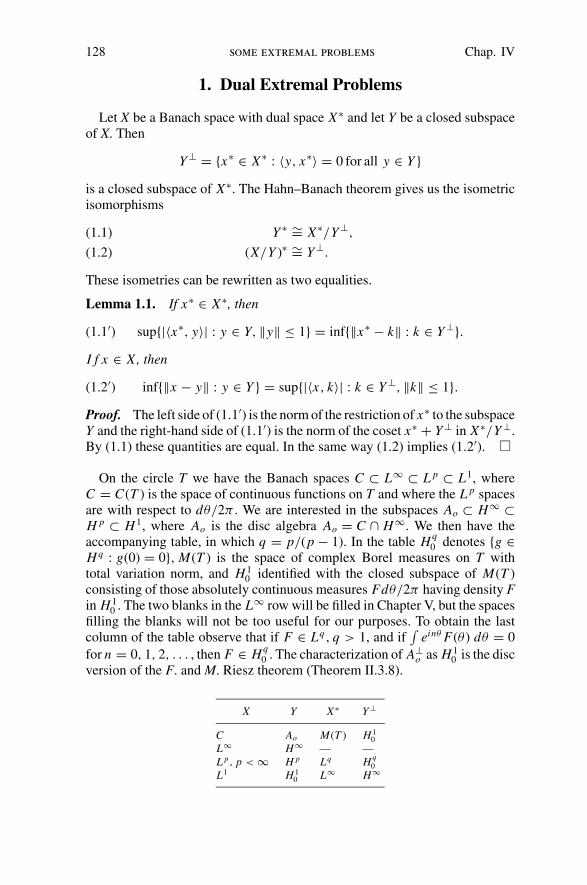
128 some extremal problems Chap. IV
1. Dual Extremal Problems
Let X be a Banach space with dual space X∗ and let Y be a closed subspaceof X. Then
Y ⊥ = {x∗ ∈ X∗ : 〈y, x∗〉 = 0 for all y ∈ Y }is a closed subspace of X∗. The Hahn–Banach theorem gives us the isometricisomorphisms
Y ∗ ∼= X∗/Y ⊥,(1.1)
(X/Y )∗ ∼= Y ⊥.(1.2)
These isometries can be rewritten as two equalities.
Lemma 1.1. If x∗ ∈ X∗, then
sup{|〈x∗, y〉| : y ∈ Y, ‖y‖ ≤ 1} = inf{‖x∗ − k‖ : k ∈ Y ⊥}.(1.1′)
I f x ∈ X, then
inf{‖x − y‖ : y ∈ Y } = sup{|〈x, k〉| : k ∈ Y ⊥, ‖k‖ ≤ 1}.(1.2′)
Proof. The left side of (1.1′) is the norm of the restriction of x∗ to the subspaceY and the right-hand side of (1.1′) is the norm of the coset x∗ + Y ⊥ in X∗/Y ⊥.By (1.1) these quantities are equal. In the same way (1.2) implies (1.2′).
On the circle T we have the Banach spaces C ⊂ L∞ ⊂ L p ⊂ L1, whereC = C(T ) is the space of continuous functions on T and where the L p spacesare with respect to dθ/2π . We are interested in the subspaces Ao ⊂ H∞ ⊂H p ⊂ H 1, where Ao is the disc algebra Ao = C ∩ H∞. We then have theaccompanying table, in which q = p/(p − 1). In the table Hq
0 denotes {g ∈Hq : g(0) = 0}, M(T ) is the space of complex Borel measures on T withtotal variation norm, and H 1
0 identified with the closed subspace of M(T )consisting of those absolutely continuous measures Fdθ/2π having density Fin H 1
0 . The two blanks in the L∞ row will be filled in Chapter V, but the spacesfilling the blanks will not be too useful for our purposes. To obtain the lastcolumn of the table observe that if F ∈ Lq , q > 1, and if
∫einθ F(θ ) dθ = 0
for n = 0, 1, 2, . . . , then F ∈ Hq0 . The characterization of A⊥
o as H 10 is the disc
version of the F. and M. Riesz theorem (Theorem II.3.8).
X Y X∗ Y ⊥
C Ao M(T ) H 10
L∞ H∞ — —L p, p < ∞ H p Lq Hq
0
L1 H 10 L∞ H∞

Sect. 1 dual extremal problems 129
Theorem 1.2. Let 1 ≤ p < ∞, and let f ∈ L p, /∈ H p. Then the distancefrom f to H p is
dist( f, H p) = infg∈H p
‖ f − g‖p
(1.3)
= sup
{∣∣∣∣
∫f F
dθ
2π
∣∣∣∣ : F ∈ Hq
0 , ‖F‖q ≤ 1
}
.
There exists unique g ∈ H p such that dist( f, H p) = ‖ f − g‖p and there existsunique F ∈ Hq
0 , ‖F‖q = 1 such that∫
f Fdθ
2π= dist( f, H p).(1.4)
Proof. The identity (1.3) follows from (1.2′). Let gn ∈ H p be such that ‖ f −gn‖p → dist( f, H p). The Poisson integrals of f − gn are bounded on anycompact subset of the disc, so by normal families there is an analytic functiong on D such that gn(z) → g(z), z ∈ D, if we replace {gn} by a subsequence.Taking means over circles of radius r < 1, we see that g ∈ H p and that ‖ f −g‖p ≤ lim ‖ f − gn‖p. Thus ‖ f − g‖p = dist( f, H p) and there exists at leastone best approximation g ∈ H p.
Let Fn ∈ Hq0 , ‖Fn‖q ≤ 1, be such that
∫f Fndθ/2π → dist( f, H p). Since
1 < q ≤ ∞, the Banach–Alaoglu theorem can be used to obtain a weak-star limit point F of {Fn}. Then ‖F‖q ≤ 1, F ∈ Hq
0 , and∫
f Fdθ/2π =dist( f, H p). Since
∫gF dθ = 0, we have
dist( f, H p) =∫
( f − g)F dθ/2π ≤ ‖ f − g‖p‖F‖q ≤ ‖ f − g‖p.(1.5)
Equality must hold throughout this chain of inequalities. This means‖F‖q = 1,and there exists a dual extremal function F for which (1.4) holds.
Now let g ∈ H p be any best approximation of f and let F ∈ Hq0 be any dual
extremal function. Because equality holds in (1.5), the conditions for equalityin Holder’s inequality give us
f − g
‖ f − g‖p= F |F |q−2 and F = ( f − g)
| f − g|p−2
‖ f − g‖p−1p
when p > 1. When p = 1 we get
( f − g)F = | f − g|instead.
Let p > 1. Since |F | > 0 almost everywhere, the first equation shows thatg is unique. Since F ∈ Hq
0 is determined by its values on any set of positivemeasure, the second equation shows that F is unique.
Similarly, when p = 1, the third equation shows that F is unique. The thirdequation then shows that Im(gF) is unique. Since gF ∈ H 1
0 , this determinesgF uniquely, and then g is determined almost everywhere because |F | > 0almost everywhere.
130 some extremal problems Chap. IV
Note that the best approximation g ∈ H p and the dual extremal functionF ∈ Hq
0 , ‖F‖q = 1, are characterized by the relation∫
( f − g)Fdθ
2π= ‖ f − g‖p‖F‖q = ‖ f − g‖p,(1.6)
which is (1.5) with equality. Sometimes it is possible to compute dist( f, H p)by finding solutions F and g of (1.6) (see Exercise 3).
When p = ∞ some of the conclusions of the theorem can be rescued if weuse the bottom row of the table instead of the second row, and use (1.1′) insteadof (1.2′).
Theorem 1.3. If f ∈ L∞, then the distance from f to H∞ is
dist( f, H∞) = infg∈H∞
‖ f − g‖∞ = sup
{∣∣∣∣
∫f F
dθ
2π
∣∣∣∣ : F ∈ H 1
0 , ‖F‖1 ≤ 1
}
.
There exists g ∈ H∞ such that ‖ f − g‖∞ = dist( f, H∞). If there exists F ∈H 1
0 , ‖F‖1 ≤ 1, such that
dist( f, H∞) =∫
f Fdθ
2π,
then the best approximation g ∈ H∞ is unique and
| f − g| = dist( f, H∞)
almost everywhere.
Proof. The dual expression for the distance follows from (1.1′). Just as inthe proof of Theorem 1.2, a normal families argument shows there is a bestapproximating function g ∈ H∞. If a dual extremal function F ∈ H 1
0 exists,then
dist( f, H∞) =∫
( f − g)Fdθ
2π= ‖ f − g‖∞‖F‖1,
so that
( f − g)
dist( f, H∞)= ( f − g)
‖ f − g‖∞= F
|F |(1.7)
almost everywhere, and there is a unique best approximation g.
If a dual extremal function F exists, (1.7) does not imply that F is unique.But it does, of course, imply that the argument of F is unique.
Example 1.4. Let f (0) = e−2iθ . Taking F0(θ ) = e2iθ we see that
1
2π
∫f F0dθ = 1.

Sect. 1 dual extremal problems 131
Hence dist( f, H∞) = 1 and F0 is a dual extremal function. However
Fα(z) = z(z + α)(1 + αz)
1 + |α|2 , |α| < 1,
is another dual extremal function. In this problem the best approximatingfunction is g = 0.
Example 1.5. Let
f (θ ) =⎧⎨
⎩
1, 0 < θ < π/2,
0, π/2 < θ ≤ 3π/2,
−1, 3π/2 < θ ≤ 2π.
If there were g ∈ H∞ such that ‖ f − g‖∞ < 1, then Re g > δ > 0 on (0, π/2)and Re g < −δ < 0 on (−π/2, 0). Hence
limε→0
1
π
∫
|θ |>ε
Re g(θ )
θdθ = +∞.
Except for bounded error terms, this integral represents − limr→1 Im g(r ).Thus there is no such bounded g, and so dist( f, H∞) = 1 and g = 0 is onebest approximation. Now let g be the conformal mapping of D onto the halfdisc D ∩ {Im z > 0}. We can arrange that g(1) = 0, g(i) = 1, and g(−i) = −1.Then by checking the values of g along the three arcs on which f is constant,we see that ‖ f − g‖∞ = 1. Hence there is not a unique best approximation tof ∈ H∞. By Theorem 1.3 there is no dual extremal function F ∈ H 1
0 .
It is interesting to notice where the proof of Theorem 1.2 breaks down inExample 1.5. By the bottom row of the table there are Fn ∈ H 1
0 , ‖Fn‖1 ≤ 1,such that
∫f Fndθ/2π → 1. As linear functionals on L∞, the Fn have some
weak-star limit point σ ∈ (L∞)∗, and σ is orthogonal to H∞. In Chapter Vwe shall see that σ is a complex measure on a compact Hausdorff space, themaximal ideal space of L∞. However, σ is not weakly continuous on L∞; thatis, σ cannot be represented as σ (h) = ∫
hFdθ with F ∈ L1. Otherwise wecould conclude that |F | = 1 almost everywhere. In fact, in a sense to be madeprecise in Chapter V, σ is singular to dθ , which means, in classical language,that Fn(z) → 0, z ∈ D. The absence of a dual extremal function F ∈ H 1
0 isoften the central difficulty with an H∞ extremal problem. We confront thisdifficulty again in Section 4.
If the function f ∈ L∞ is continuous, there is a dual extremal function Fand the best approximation g is unique.
Lemma 1.6. If f ∈ C, then
dist( f, H∞) = dist( f, Ao) = infg∈Ao
‖ f − g‖∞.
Proof. There exists g ∈ H∞ such that ‖ f − g‖∞ = dist( f, H∞). Let fr =f ∗ Pr be the Poisson integral of f and let gr = g ∗ Pr . Since ‖Pr‖1 = 1 we
132 some extremal problems Chap. IV
have
‖ fr − gr‖∞ = ‖( f − g) ∗ Pr‖∞ ≤ ‖ f − g‖∞.
But gr ∈ Ao, and ‖ f − fr‖∞ < ε if 1 − r is small. Thus
dist( f, Ao) ≤ limr
‖ f − gr‖∞ ≤ ‖ f − g‖∞ = dist( f, H∞).
The reverse inequality is clear since H∞ ⊃ Ao.
We write H∞ + C for the set of functions g + h, g ∈ H∞, h ∈ C .
Theorem 1.7. If f ∈ H∞ + C, then there exists F ∈ H 10 , ‖F‖1 = 1, such
that
1
2π
∫f F dθ = dist( f, H∞),(1.8)
and there exists unique g ∈ H∞ such that ‖ f − g‖∞ = dist( f, H∞).
Proof. Write f = g + h, g ∈ H∞, h ∈ C . Then dist( f, H∞) = dist(h, H∞)and we can assume that f is continuous. By Theorem 1.3 there are Fn ∈H 1
0 , ‖Fn‖1 ≤ 1, such that
1
2π
∫f Fndθ → dist( f, H∞).
Taking a subsequence we can assume Fn(z) → F(z), z ∈ D, where F ∈H 1
0 , ‖F‖1 ≤ 1. This gives convergence of the Fourier coefficients, so that forall trigonometric polynomials p(θ ),
∫Fn p
dθ
2π→
∫Fp
dθ
2π.
Taking ‖ f − p‖∞ small we see that
dist( f, H∞) =∫
F fdθ
2π.
Hence (1.8) holds and Theorem 1.3 now implies that f has a unique bestapproximation in H∞.
As an application we reprove some results from Chapter I, Section 2.
Corollary 1.8. Let z1, z2, . . . , zn be distinct points in D, and letw1, w2, . . . , wn be complex numbers. Among all f ∈ H∞ such that
f (z j ) = w j , 1 ≤ j ≤ n,(1.9)
there is a unique function f of minimal norm. This function has the form cB(z)where B(z) is a Blaschke product of degree at most n − 1.

Sect. 1 dual extremal problems 133
Corollary 1.9. Let zn+1 ∈ D be distinct from z1, z2, . . . , zn. Assume (1.9)has a solution f ∈ H∞ with ‖ f ‖∞ ≤ 1. Among such solutions let f0 he onefor which | f (zn+1)| is largest. Then f0 is uniquely determined by its valuef0(zn+1) and f0 is a Blaschke product of degree at most n.
Corollary 1.9 is a simple consequence of Corollary 1.8. By normal familiesthere exists an extremal function f0, ‖ f0‖∞ ≤ 1. Let wn+1 = f0(zn+1). If f ∈H∞ interpolates (1.9) and if also
f (zn+1) = wn+1,
then ‖ f ‖∞ ≥ 1, because otherwise for some λ, |λ| small,
g = f + λ
n∏
j=1
z − z j
1 − z j z
is a function satisfying (1.9) such that ‖g‖ ≤ 1 and |g(zn+1)| > | f0(zn+1)|.Hence f0 has minimal norm among the functions interpolating w1, . . . , wn+1
at z1, . . . , zn+1.
Proof of Corollary 1.8. Let B0 be the Blaschke product with zeros z1, . . . zn ,and let f0 be a polynomial that does the interpolation (1.9). The minimal normof the functions in H∞ satisfying (1.9) is
infg∈H∞
‖ f0 − B0g‖∞ = infg∈H∞
‖B0 f0 − g‖∞.
Since B0 f0 ∈ C , there is a unique interpolating function f ∈ H∞ of minimalnorm and there is F ∈ H 1
0 , ‖F‖1 = 1, such that∫
f B0 Fdθ
2π= ‖ f ‖∞.
Hence | f | = | f B0| = ‖ f ‖∞ almost everywhere, and
f F/B0 ≥ 0(1.10)
almost everywhere.
Lemma 1.10. If G ∈ H 1 is real almost everywhere on an arc I ⊂ T , then Gextends analytically across I.
Proof. On |z| > 1 define G(z) = G(1/z). This is an H 1 function on |z| > 1with nontangential limits G(θ ) at almost every point of I . Let ζ ∈ I and centerat ζ a disc so small that ∩ T ⊂ I . Let V = ∩ D, W = ∩ {|z| > 1}.Since we are dealing with H 1 functions, we have for w ∈ \T ,
1
2π i
∫
∂
G(z)
z − wdz = 1
2π i
∫
∂V
G(z)
z − wdz + 1
2π i
∫
∂W
G(z)
z − wdz = G(w).
This shows that G can be continued across I.

134 some extremal problems Chap. IV
To complete the proof of Corollary 1.8, notice that G = f F/B0 is an H 1
function on the annulus r < |z| < 1 if r > |z j |. Using (1.10) and using thelemma locally, we see that G is analytic across T, and that G is in fact arational function. Since B0G is analytic across T, and since f/‖ f ‖∞ is aninner function, Theorem II.6.3 shows that f is analytic across T. Consequentlyf/‖ f ‖∞ is a Blaschke product of finite degree, and F is a rational function.Now B0 has n zeros in D and F has a zero at z = 0. By (1.10) and the argumentprinciple, it follows that f has at most n − 1 zeros.
In Corollary 1.8 the extremal function f (z) = cB(z) can have fewer than n −1 zeros. For example, suppose g is the function of minimum norm interpolating
g(z j ) = w j , 1 ≤ j ≤ n − 1,
and take wn = g(zn). Then f = g has at most n − 2 zeros. Similarly, the ex-tremal function in Corollary 1.9 can have fewer than n zeros. However, if the in-terpolation (1.9) has two distinct solutions f1, f2 with ‖ f1‖∞ ≤ 1, ‖ f2‖∞ ≤ 1,then the extremal function f0 in Corollary 1.9 is a Blaschke product of degreen. For the proof, notice that (1.9) then has a solution f with ‖ f ‖∞ < 1, by theuniqueness asserted in Corollary 1.8. Then by Rouche’s theorem, f0 and f0 − fhave the same number of zeros in |z| < 1. Since f0(z j ) = f (z j ), 1 ≤ j ≤ n,it follows that f0 has at least n zeros in |z| < 1.
Corollary 2.4 Chapter I, contains more information than we have obtainedhere, but the duality methods of this section apply to a wider range of problems.
2. The Carleson–Jacobs Theorem
Let f (θ ) ∈ C . From Theorem 1.7 we know there is a unique function g ∈H∞ such that
‖ f − g‖∞ = dist( f, H∞).
We want to know when the best approximation g(θ ) is continuous on T. Al-though necessary and sufficient conditions on f (θ ) are not known, there isa sharp result parallel to Theorem 1.3 of Chapter III about the continuity ofconjugate functions. Recall that the modulus of continuity of f (θ ) is
ω(δ) = ω f(δ) = sup{| f (θ ) − f (ϕ)| : |θ − ϕ| < δ}.Theorem 2.1. If f (θ ) is Dini continuous, that is, if, for some ε > 0
∫ t
0
ω(t)
tdt < ∞,
then the best approximation g ∈ H∞ to f is continuous on T.
Theorem 2.2. Let ω(t) be a continuous nondecreasing function such thatω(0) = 0 and ω(t1 + t2) ≤ ω(t1) + ω(t2). If
∫0ω(t)/t dt = ∞, then there is

Sect. 2 the carleson–jacobs theorem 135
f (θ ) ∈ C such that ω f (δ) ≤ ω(δ) but such that the best approximation to f inH∞ is not continuous.
We prove Theorem 2.1 first. In doing so we can assume
‖ f − g‖∞ = dist( f, H∞) = 1.
By Theorem 1.7, there is F ∈ H 10 , ‖F‖1 = 1, such that
( f − g)F = |F | a.e(2.1)
All information used in the proof will follow from (2.1) and the continuity off. We need two lemmas.
Lemma 2.3. Let G = u + iv ∈ H 1 and let I be an arc on T such that almosteverywhere on I
u > 0, |v| ≤ αu,
where α > 0. Let J be a relatively compact subarc of I and let V be the domain{reiθ : r0 < r < 1, 0 ∈ J }. Then G ∈ H p(V ) if
arctan α < π/2p.
The statement G ∈ H p(V ) means that |G|p has a harmonic majorant in V.
Proof. Recall from Corollary 2.5 in Chapter III that an H 1 function whoseboundary values lie in the sector S = {x > 0, |y| < αx} is in H p if arctanα < π/2p. Enlarging J, we may assume G has a finite radial limit at the end-points of J. Then M = sup{|G(z)| : z ∈ ∂V, |z| < 1} is finite, and
g = M(1 + 1/α) + G
has, at almost every point of ∂V , boundary value in the cone S (see Figure IV.1).
Figure IV.1. S = {|y| < αx, x > 0}. On ∂V, g has values in the union of the disc and the shadedcone.
136 some extremal problems Chap. IV
Because g ∈ H 1(V ), the Poisson integral formula (applied after conformallymapping V onto the unit disc) shows that g(V ) ⊂ S. By Corollary III.2.5 andthe conformal invariance of the definition of H p(V ), we see that g ∈ H p(V )and hence that G ∈ H p(V ).
Lemma 2.4. Let f (θ ) ∈ C, let g(θ ) ∈ H∞ and let F(θ ) ∈ H 10 be functions
such that (2.1) holds. Then
(a) F ∈ H p for all p < ∞, and(b) if τ ∈ [0, 2π ] and if
fτ = f − f (τ ), gτ = g − f (τ ),
then there is δ > 0 and r0 > 0 such that |gr (z)| ≥ 12
on
Wτ = {reiθ : |θ − τ | < δ/2, r0 < r < 1}.Proof. To prove (a) let p < ∞ and let ε > 0 satisfy arctan(ε/(1 − ε)) <
π/2p. Choose δ so that | f (θ ) − f (τ )| < ε when |θ − τ | < δ. Then on Iτ ={θ : |θ − τ | < δ}, we have by (2.1)
−gτ F = ( f − g)F − fτ F = |F | − fτ F.
Consequently, Re(−gτ F) > 0 and |Im gτ F | < ε/(1 − ε) Re(−gτ F) almosteverywhere on Iτ . By Lemma 2.3 we have gτ F ∈ H p(Wτ ). If we replace Wτ
by the intersection of two discs whose boundaries cross inside Iτ , a simpleconformal mapping can be used to show
∫
|θ−τ |<δ/2
|gτ F |pdθ < ∞.
Since |gτ | ≥ ‖ f − g‖∞ − ω(δ) ≥ 1 − ε on Iτ , this means∫|θ−τ |<δ/2
|F |pdθ <
∞, so that F ∈ L p. Hence F ∈ H p by Corollary 11.4.3.To prove (b) first take ε so small that on Iτ
−gτ F = exp(u + iv),
where ‖v‖∞ < π/4. then
h = exp(−ivχIτ + vχIτ )
is in H 2 by Corollary III.2.6. The H 1 function gτ Fh is real on Iτ . By Lemma1.10 and Theorem II.6.3, the inner factor of gτ Fh is analytic across It . Conse-quently, the inner factor of gτ is analytic across Iτ . The representation for-mula for outer functions then shows |gτ (z)| ≥ 3
4in a region {r0(τ ) < r <
1, |θ − τ | < δ/2}. Since gσ (z) = gτ (z) − ( f (σ ) − f (τ )), we have |gσ (z)| > 12
on the same region if |σ − τ | < δ. This means we may choose r0(τ ) indepen-dent of τ , and thus (b) is proved.

Sect. 2 the carleson–jacobs theorem 137
Proof of Theorem 2.1. By Lemma 2.4(b), gτ (z) has a single-valued loga-rithm on Wτ , and the logarithm is defined by
log gτ (z) = 1
2π
∫
|θ−τ |<δ
log |gτ (θ )|eiθ + z
eiθ − zdθ + Rτ (z),(2.2)
where Rτ (z) is the same integral over |θ − τ | ≥ δ plus the logarithm of theinner factor of gτ (z). Since |gτ (z)| ≥ 1
2on Wτ , the inner factor is bounded
below on Wτ and it is analytic across {eiθ : |θ − τ | < δ/2}. Hence there isr1 > 0 such that Rτ (z) is bounded and analytic on τ = {|z − eiτ | < r1}. Theradius r1 and the bound sup {|Rτ (z)| : z ∈ τ } are independent of τ .
Because | fτ − gτ | = 1, we have
1 − |gτ |2 = | fτ |2 − 2 Re fτ gτ ≤ Aω(|θ − τ |),so that
| log |gτ (θ )‖ ≤ cω(|θ − τ |).Let �(τ ) be the truncated cone
�(τ ) ={
z :|z − eiτ |1 − |z| ≤ 2, r2 < |z| < 1
}
,
where r2 > 0 is such that �(τ ) ⊂ τ . For z ∈ �τ ,
∣∣∣∣eiθ + z
eiθ − z
∣∣∣∣ ≤ C
|θ − τ | ,
so that (2.2) yields
| log gτ (z) − Rτ (z)| ≤ C∫ δ
0
ω(t)
tdt, z ∈ �(τ ).
By Schwarz’s lemma and the uniform bound on Rτ (z), |Rτ (z) − Rτ (w)| ≤c|z − w|, z, w ∈ �(τ ). Therefore
|gτ (z) − gτ (w)| ≤ C |z − w| + η(δ),
z, w ∈ �τ , where η(δ) → 0(δ → 0).Now let τ and σ be so close together that there is a point z ∈ �(τ ) ∩ �(σ ).
Taking nontangential limits, we then obtain (when 1 − |z| is small)
|g(eiτ ) − g(eiσ )| ≤ |g(eiτ ) − g(z)| + |g(z) − g(eiσ )|≤ |gτ (eiτ ) − gτ (z)| + |gσ (z) − gσ (eiσ )|≤ 2η(δ) + |eiτ − z| + |eiσ − z|≤ 2η(δ) + C |σ − τ |.
138 some extremal problems Chap. IV
Fixing δ > 0 with 2η(δ) < ε, we conclude that
limσ→τ
|g(eiσ ) − g(eiτ )| < ε,
which means that g is continuous.
Now let ω(t) satisfy the hypotheses of Theorem 2.2.
Lemma 2.5. Let δ > 0. Let
f (eit ) ={
ω(t), 0 ≤ t ≤ δ,
0, −δ ≤ t < 0.
Extend f (eit ) to be smooth on δ < |t | < π and continuous on [−π, π] withf (−π ) = f (π ). Let g ∈ H∞ be the best approximation of f. If g is continuous,then
g(1) = ± i‖ f − g‖∞.
Proof. Since f is real, f /∈ H∞ and ‖ f − g‖∞ > 0. We may suppose‖ f − g‖∞ = 1, so that | f − g| = 1 on T. We must prove Re g(1) = 0. Since| f − g| = 1, log |g(t)| = 0 on −δ < t < 0. Suppose Re g(1) > 0. Then for0 < t < δ,
log |g| = − log
∣∣∣∣g − f
g
∣∣∣∣ ≤ − log
(
1 − f Re g
|g|2)
≤ −Cω(t).
Similarly, if Re g(1) < 0, then on 0 < t < δ, log |g| ≥ Cω(t). Moreover, g hasa continuous logarithm on {|z − 1| < δ, |z| ≤ 1}, again because | f − g| = 1.However, if Re g(1) �= 0, then by Lemma III.1.2,
limr→1
| arg g(r )| =∣∣∣∣c + lim
ε→0
1
π
∫
|t |>ε
log |g(t)|t
dt
∣∣∣∣
≤ c + C limε→0
1
π
∫
|t |>ε
ω(t)
tdt = +∞.
This contradiction shows g(1) = ±i .
To prove Theorem 2.2 let δn = 2−n , and let
ωn(t) = ω
(δn
2−
∣∣∣∣δn + δn−1
2− t
∣∣∣∣
)
on [δn, δn−1], ωn(t) = 0 off [δn, δn−1]. Let
f (eit ) =∞∑
k=1
1
2ω4k+1(t) + i
∞∑
k=1
1
2ω4k+3(t).
Sect. 3 the helson–szego theorem 139
Then f 2 is real, so that f /∈ H∞. It is not hard to verify that ω f (δ) ≤ ω(δ). Ifg is the best approximation of f, then Lemma 2.5 says that
g(eiδ4k+1 ) = ±i‖ f − g‖∞, g(eiδ4k+3 ) = ±‖ f − g‖∞.
Thus g(eit ) is not continuous at t = 0.
3. The Helson–Szego Theorem
Let p(θ ) be a trigonometric polynomial on the circle T and let p(θ ) be itsconjugate function. Then p is another trigonometric polynomial, normalizedto have mean zero. In this section we give the Helson–Szego characterizationof those positive measures μ on T for which
∫| p(θ )|2 dμ(θ ) ≤ K
∫|p(θ )|2 dμ(θ )
for every trigonometric polynomial p(θ ). This of course means that conjugationextends to a bounded operator on L2(μ). In Chapter VI a completely differentcharacterization of such measures μ will be given, and these two results willbe merged to provide a description of the uniform closure in L∞ of the spaceof real parts of H∞ functions.
First we need the famous and beautiful theorem of Szego. Let F be the setof polynomials in z vanishing at z = 0. Restricted to the circle, F coincideswith the set of trigonometric polynomials of the form
∑n>0 aneinθ .
Theorem 3.1 (Szego). Let dμ be a finite positive measure on the circle. Write
dμ = w dθ/2π + dμs,
where dμs is singular to dθ . Then
inff ∈F
∫|1 − f |2dμ = exp
1
2π
∫log w dθ.(3.1)
Notice that if the infimum in (3.1) is zero, then F is dense in L2(μ), becauseby induction e−iθ , e−2iθ , . . . also then lie in the closure of F .
Proof. We first dispense with the singular part μs . By Exercise 2, ChapterIII, there are polynomials pn in F such that ‖pn‖∞ ≤ 1, pn → 1 a.e. dμs andpn → 0 a.e. dθ . For any f0 ∈ F we have f0 + pn(1 − f0) ∈ F , so that
infF
∫|1 − f |2dμ ≤ lim
n
∫|1 − ( f0 + pn(1 − f0))|2dμ
= limn
∫|1 − f0|2|1 − pn|2dμ
=∫
|1 − f0|2w dθ
2π.

140 some extremal problems Chap. IV
Since dμ ≥ w dθ/2π , the reverse inequality is trivial, so that
infF
∫|1 − f |2dμ = inf
F
∫|1 − f |2w dθ
2π,
and we can assume μ is absolutely continuous.Write ϕ = log w. Assume for the moment that
∫ϕ dθ > −∞. Let ψ = ϕ
be the conjugate function and let
G = exp1
2(ϕ + iψ).
Then G is an outer function in H 2, |G|2 = w almost everywhere, and
G2(0) = exp
∫ϕ
dθ
2π
is the right side of (3.1). For f ∈ F have
1
2π
∫|1 − f |2w dθ = 1
2π
∫|(1 − f )2G2| dθ
≥ |(1 − f (0))2G2(0)| = exp1
2π
∫ϕ dθ.
because (1 − f )2G2 is in H1.Now G is an outer function, and so by Beurling’s theorem there are polynomi-
als pn(z) such that pnG converges to the constant function G(0) in H 2. Thenpn(0)G(0) → G(0) �= 0, so that pn(0) → 1 and we can assume pn(0) = 1.Thus we can take pn = 1 − fn, fn ∈ F . But then
limn
1
2π
∫|1 − fn|2w dθ = lim
n
1
2π
∫|pnG|2 dθ
= 1
2π
∫|G(0)|2 dθ = exp
1
2π
∫ϕ dθ.
Therefore (3.1) is proved when log w ∈ L1.Now assume
∫log w dθ = −∞. For ε > 0, log(w + ε) is integrable, and
so by the preceding
inff ∈F
1
2π
∫|1 − f |2w dθ ≤ inf
f ∈F1
2π
∫|1 − f |2(w + ε) dθ
= exp1
2π
∫log(w + ε) dθ.
The last expression tends to zero with ε and we have
inff ∈F
1
2π
∫|1 − f |2w dθ = 0
if∫
log w dθ = −∞.

Sect. 3 the helson–szego theorem 141
Turning to the work of Helson and Szego, we again let
dμ = w dθ/2π + dμs
be a finite positive measure on T. Let G be the space of conjugate analytictrigonometric polynomials
g = b0 + b1e−iθ + b2e−2iθ + . . . ,
and let
ρ = sup
∣∣∣∣
∫f g dμ
∣∣∣∣,
where f and g range overF andG respectively but where f and g are constrainedby
∫| f |2 dμ ≤ 1,
∫|g|2 dμ ≤ 1.
It is clear that 0 ≤ ρ ≤ 1. The spaces F and G are orthogonal in L2(μ) if and
only if ρ = 0. If there is a nonzero vector in both the L2(μ) closures F and G,
then ρ = 1. If ρ < 1 the closed subspaces F and G of L2(μ) are said to be atpositive angle, and the angle between the subspaces is cos−1 ρ. When F and
G are at positive angle, F + G is closed in L2(μ) and
‖ f ‖2 + ‖g‖2 ≤ (1 − ρ)−1‖ f + g‖2,
f ∈ F , g ∈ G, so that F + G is the Banach space direct sum of F and G.Examples exist of closed subspaces F and G such that F ∩ G = {0} but suchthat ρ = 1 and F + G is not closed. (See Exercise 9.)
Theorem 3.2 (Helson–Szego). The subspaces F and G are at positive angleif and only if
μs = 0,(3.2)
and
log w = u + v.(3.3)
where u ∈ L∞, v ∈ L∞ and ‖v‖∞ < π/2.
Proof. First let us show that (3.2) is necessary. Suppose dμs > 0. By Exercise2, Chapter III, there are pn ∈ F such that |pn| ≤ 1, pn → 1 almost everywheredμs, and pn → 0 almost everywhere dθ . Then gn = pn ∈ G, and
∫pngndμ →
∫dμs,
while ∫|pn|2 dμ =
∫|gn|2dμ →
∫dμs.
Scaling pn and gn to have unit norm in L2(μ), we see that ρ = 1.

142 some extremal problems Chap. IV
We can now assume μ is absolutely continuous, μ = w dθ/2π . We can alsoassume that
∫log w
dθ
2π> −∞,
because otherwise F is dense in L2(μ) by Szego’s theorem, so that G ⊂ Fand ρ = 1, while on the other hand, (3.3) obviously fails.
Let ϕ = log w, let ψ = ϕ and let G = exp 12(ϕ + iψ) be as in the proof of
Theorem 3.1. Let H = G2. Then G ∈ H 2, H ∈ H 1, G and H are outer, and
|G|2 = |H | = w.
Then we have
ρ = sup
∣∣∣∣
1
2π
∫( f G)(gG)e−iψdθ
∣∣∣∣,
where the supremum is taken over all f ∈ F and g ∈ G such that
1
2π
∫| f G|2dθ = 1
2π
∫|gG|2 dθ = 1.
By Beurling’s theorem the set { f G : f ∈ F } is dense in H 20 and the set {gG :
g ∈ G} is dense in H 2. Since every F ∈ H 10 can be factored as F = F1 F2,
where F1 ∈ H 20 , F2 ∈ H 2, and
‖F1‖2 = ‖F2‖2 = ‖F‖1,
we have
ρ = sup
{∣∣∣∣
∫Fe−iψ dθ
2π
∣∣∣∣ : F ∈ H 1
0 , ‖F‖1 ≤ 1
}
.
By duality this means
ρ = infg∈H∞
‖e−iψ − g‖∞.
Lemma 3.3. If ψ is a real measurable function, then
infg∈H∞
‖e−iψ − g‖ < 1
if and only if there are ε > 0 and h ∈ H∞ such that
|h| ≥ ε a.e.(3.4)
|ψ + arg h| ≤ π/2 − ε (modulo 2π ).(3.5)
Proof. Notice that if g ∈ H∞ and ‖e−iψ − g‖∞ < 1 then g satisfies (3.4)and (3.5). On the other hand, if (3.4) and (3.5) hold for h, then for a smallλ > 0, ‖e−iψ − λh‖∞ < 1. (The proof is illustrated in Figure IV.2.)

Sect. 3 the helson–szego theorem 143
Figure IV.2. The proof of Lemma 3.3. The values of h lie in the cone |ψ + arg z| < π/2 − ε,and in |z| > ε. The shaded region includes all values λh and is contained in |z − eiψ | < d < 1.
Now assume ρ < 1. Then there is h ∈ H∞ with (3.4) and (3.5). Since argH = ψ we have
| arg(h H )| <π
2− ε,
and the H 1 function hH has a well-defined logarithm. Letting v = − arg(h H ),we have ‖v‖∞ < π/2 − ε and
log |h H | = v.
By (3.4) u = − log |h| is bounded. Hence
log w = log |H | = log |h H | − log |h| = u + v,
and (3.3) holds.Conversely, suppose that μ is absolutely continuous and that log w has the
form (3.3). We can then assume u = 0, because the property ρ = 1 is notchanged by multiplying w by a positive bounded function bounded away fromzero. (See Exercise 10.) Then in the above discussion
ψ = ϕ = −v.
Since ‖v‖∞ < π/2, the constant function g = cos(‖v‖∞) has
‖e−iψ − g‖∞ < 1,
so that ρ < ‖e−iψ − g‖ < 1.

144 some extremal problems Chap. IV
Theorem 3.4. Let μ be a positive finite measure on the circle. Then there isa constant K such that
∫| p|2dμ ≤ K 2
∫|p2|dμ(3.6)
for all trigonometric polynomials if and only if μ is absolutely continuous,dμ = w dθ/2π , and
log w = u + v,
where u ∈ L∞, v ∈ L∞, and ‖v‖∞ < π/2.
Proof. We show the conjugation operator is bounded in L2(μ) if and only if
the subspaces F and G are at positive angle in L2(μ). With Theorem 3.2 thatwill prove the result.
Let T be the operator defined on trigonometric polynomials by
T (p) = 1
2{(p − a0) + i p},
where a0 = a0(p) = ∫p dθ/2π . Thus
T (∑
aneinθ ) =∑
n>0
aneinθ .
Since (p − a0(p)) = (− p)∼, we see that T is bounded with respect to the L2(μ)norm whenever (3.6) holds. Conversely if
∫|T (p)|2dμ ≤ C2
∫|p|2 dμ,(3.7)
then (3.6) is true for real trigonometric polynomials, and therefore for alltrigonometric polynomials. Thus (3.7) is equivalent to (3.6).
Every trigonometric polynomial p(θ ) has the form p = f − g, where f ∈F , g ∈ G, and
T (p) = T ( f − g) = f.
Hence if T is bounded and if∫ | f |2dμ = ∫ |g|2dμ = 1, then by (3.7) we have
C−2 ≤∫
| f − g|2dμ = 2 − 2 Re
∫f g dμ.
Letting∫
f g dμ approach ρ, we calculate that ρ < 1 − 1/2C2.On the other hand, if ρ < 1 and if f ∈ F , g ∈ G, then
∫| f − g|2dμ ≥
∫| f |2dμ +
∫|g|2dμ − 2ρ
(∫| f |2 dμ
)1/2 (∫|g|2 dμ
)1/2
≥ (1 − ρ)
(∫| f |2 dμ +
∫|g|2 dμ
)

Sect. 4 interpolating functions of constant modulus 145
and∫
| f |2 dμ =∫
|T ( f − g)|2 dμ ≤ (1 − ρ)−1
∫| f − g|2 dμ.
Hence T is bounded if ρ < 1.
4. Interpolating Functions of Constant Modulus
Let {z j } be a sequence of distinct points in D, and let {w j } be a sequence ofcomplex numbers. Assume there is f0 ∈ H∞ solving the interpolation problem
f (z j ) = w j , j = 1, 2, . . . .(4.1)
If there are finitely many points z j then by Pick’s theorem or by Corollary 1.8the interpolation (4.1) can be solved with f = cB where B is a finite Blaschkeproduct and where c is the minimum norm of all interpolating functions. Inthis section we consider the case in which there are infinitely many z j . Weassume
∑(1 − |z j |) < ∞,
a condition necessary and sufficient for (4.1) to have more than one solutionin H∞.
Theorem 4.1. (Nevanlinna). If there are two distinct functions of unit normin H∞ that do the interpolation (4.1), then there is an inner function that alsosatisfies (4.1).
If f0 fulfills (4.1) and if ‖ f0‖ < 1, then the two function hypothesis istrivially satisfied. Indeed, let B(z) be the Blaschke product with zeros {z j }.Then for some s > 0 and for some t < 0, f0 + s B and f0 + t B are two distinctinterpolating functions of norm 1. If there is exactly one function of unit normsatisfying (4.1), then this reasoning (and the theorem) show that interpolationis always possible with a function of constant modulus 1 + ε, for any ε > 0.Before proving the theorem, we mention an example indicating that there maynot be an inner function solving (4.1) when it is merely assumed that thereexists one interpolating function of norm 1.
Example 4.2. Let lim z j = 1. Let I be an open are on T containing z = 1.Let f ∈ (H∞)−1 have ‖ f ‖ = 1, | f | = 1 on I but | f | �≡ 1. Let w j = f (z j ).Then every other interpolating function for this problem has the form f −Bg, g ∈ H∞, where B is the Blaschke product with zeros z j . We claim g = 0if ‖ f − Bg‖ ≤ 1. This means there is only one interpolating function of unitnorm, namely f, and that function is not an inner function.
So assume g ∈ H∞ and ‖ f − Gg‖ ≤ 1. Then
|1 − Bg/ f | ≤ 1
146 some extremal problems Chap. IV
almost everywhere on I, so that
Re Bg/ f ≥ 0
almost everywhere on I. By Exercise 14, Chapter II, the inner factor of Bg/ fis analytic across I. If g �≡ 0, this inner factor is a multiple of B, which is notanalytic across I. So g ≡ 0.
Theorem 4.1 is a consequence of the following theorem due to Adamyan,Arov, and Krein [1968].
Theorem 4.3. Let h0 ∈ L∞. If the coset h0 + H∞ of L∞/H∞ contains twofunctions of unit norm, then it contains a function h ∈ L∞ such that |h| = 1almost everywhere.
To derive Nevanlinna’s theorem from Theorem 4.3, let h0 = B f0, where Bis the Blaschke product with zeros {z j }. If h ∈ B f0 + H∞ and if |h| = 1, thenBh is an inner function such that (Bh)(z j ) = f0(z j ), j = 1, 2, . . . .
The proof of Theorem 4.3 will be divided into two cases, although the firstcase can be subsumed under the more difficult second case. The strategy forthe proof has already been suggested by Corollary 1.9. To obtain a unimodularfunction we maximize a linear functional over
K = {h ∈ h0 + H∞ : ‖h‖ = 1}.Write
‖h0 + H∞‖ = inf{‖h0 − g‖ : g ∈ H∞}for the norm of our coset in L∞/H∞.
Case 1. ‖h0 + H∞‖ < 1. Consider the extremal problem
a = sup
{∣∣∣∣
1
2π
∫h dθ
∣∣∣∣ : h ∈ K
}
.(4.2)
By a normal family argument there is an extremal function h ∈ K such that|(1/2π )
∫h dθ | = a. We claim |h| = 1 almost everywhere.
Notice that
dist(h, H∞0 ) = inf{‖h − g‖ : g ∈ H∞, g(0) = 0} = 1,(4.3)
since otherwise h − g + ε∫
h dθ/2π, g ∈ H∞0 , ε > 0, would be a function in
K with a larger mean. On the other hand, by hypothesis we have
dist(h, H∞) = ‖h0 + H∞‖ < 1.(4.4)
Since(H 1)⊥ = H∞0 ,(4.3) gives
sup
{∣∣∣∣
∫hF
dθ
2π
∣∣∣∣ : F ∈ H 1, ‖F‖1 ≤ 1
}
= 1,(4.3′)

Sect. 4 interpolating functions of constant modulus 147
while (4.4) gives
sup
{∣∣∣∣
∫hF
dθ
2π
∣∣∣∣ : F ∈ H 1
0 , ‖F‖1 ≤ 1
}
< 1.(4.4′)
By (4.3′) there are Fn ∈ H 1, ‖Fn‖1 ≤ 1 such that∫
hFndθ
2π→ 1.(4.5)
This means
limn
|Fn(0)| > 0,(4.6)
because otherwise we would have a subsequence for which∫
hFn − Fn(0)
‖Fn − Fn(0)‖1
dθ
2π→ 1,
and this contradicts (4.4′).Now suppose there were a measurable set E of positive measure such that
|h| < λ < 1 on E. As ‖Fn‖1 ≤ 1,(4.5) then yields∫
E|Fn| dθ
2π→ 0.
Since the logarithm is concave, Jensen’s inequality now gives∫
Elog |Fn| dθ
2π→ −∞.
and as
log |Fn(0)| ≤∫
Elog |Fn| dθ
2π+
∫
T/E|Fn| dθ
2π,
we obtain log |Fn(0)| → −∞, in contradiction to (4.6).Before turning to Case 2 we digress somewhat in order to obtain further
information when ‖h0 + H∞‖ < 1.
Theorem 4.4. If ‖h0 + H∞‖ < 1, there is h ∈ h0 + H∞ and there is F ∈H 1, F �= 0 such that
h = F/|F |(4.7)
almost everywhere.
Proof. Let h and {Fn} be as in the above discussion. We claim the sequence{Fn} has a subsequence converging weakly in L1. If F is any weak limit point,then by (4.5)
∫hF dθ/2π = 1. Since ‖h‖ ≤ 1, this implies (4.7).

148 some extremal problems Chap. IV
If the sequence {Fn} has no weakly convergent subsequence, then there aremeasurable sets Ek ⊂ T such that
|Ek | → 0
but such that∣∣∣∣
∫
Ek
Fkdθ
2π
∣∣∣∣ ≥ β > 0,(4.8)
where {Fk} denotes a subsequence of the Fn (see Dunford and Schwartz [1958,p. 292]).
Lemma 4.5. If {Ek} is a sequence of measurable subsets of T such that|Ek | → 0, then there is a sequence {gk} of functions in H∞ such that
(i) supEk|gk | → 0,
(ii) gk(0) → 1, and(iii) |gk | + |1 − gk | ≤ 1 + εk ,
where limk εk = 0.
Let us assume the lemma for the moment and finish proving Theorem 4.4Let
Gk = gk Fk
1 + εk, Hk = (1 − gk)Fk
1 + εk.
Then Gk, Hk ∈ H 1. Since εk → 0, (4.5) gives us
‖Gk‖1
∫hGk
‖Gk‖1
dθ
2π+ ‖Hk‖1
∫h Hk
‖Hk‖1
dθ
2π→ 1.(4.9)
Now for k sufficiently large, ‖Hk‖1 ≥ β/2 by (4.8) and condition (i). By con-dition (iii) ‖Gk‖1 + ‖Hk‖1 ≤ 1, and (4.9) then yields
∫h Hk
‖Hk‖1
dθ
2π→ 1.
However, condition (ii) implies that lim Hk(0) = 0, and we again have a con-tradiction to (4.4′).
Proof of Lemma 4.5. Choose Ak → ∞ so slowly that Ak |Ek | → 0. Let fk
be the Poisson integral of
AkχEk + i Ak χEk .
Then fk is an analytic function in D and fk takes values only in the right halfplane. Also fk(0) = Ak |Ek | and Re fk = Ak almost everywhere on Ek . Lethk = (1 + fk)−1. Then hk maps D into the disc
|w − 12| < 1
2,(4.10)
Sect. 4 interpolating functions of constant modulus 149
and hk(0) → 1 while supEk |hk | → 0. The disc defined by (4.10) is compressedinto the ellipse defined by (iii) under the mapping w → wδ , if δ > 0 is small.
We can choose δk → 0 so slowly that gk = hδkk then satisfies conditions (i)–
(iii).
We return to the proof of Theorem 4.3.
Case 2. ‖h0 + H∞‖ = 1. By the hypothesis, there are two distinct functionsh1 and h2 in the coset h0 + H∞ such that ‖h1‖ = ‖h2‖ = 1. Since h1 �= h2
there is a point z ∈ D such that∫
h1 Pzdθ
2π�=
∫h2 Pz
dθ
2π.
Using a Mobius transformation, we can suppose z = 0, and rotating h0 we canassume
Re
∫h1
dθ
2π�= Re
∫h2
dθ
2π.(4.11)
As in Case 1, the function h ∈ h0 + H∞ with |h| = 1 almost everywhere willbe found by maximizing
Re
∫h
dθ
2π
over K = {h ∈ h0 + H∞, ‖h‖ ≤ 1}. However, this time we must use the proofof the Hahn–Banach theorem instead of that theorem itself.
Since L∞/H∞ is the dual space of H 10 , the elements h ∈ h0 + H∞ with
‖h‖ = 1 correspond naturally to the norm-preserving extensions to L1 of thelinear functional
H 10 � F →
∫h0 F
dθ
2π.
Now (4.11) says that this functional has two norm-preserving extensions whosereal parts disagree at the constant function 1 ∈ L1/H 1
0 . The proof of the Hahn–Banach theorem therefore gives us
supF∈H 1
0
{
−‖1 + F‖ − Re
∫h0 F
dθ
2π
}
= m,
infF∈H 1
0
{
‖1 + F‖ − Re
∫h0 F
dθ
2π
}
= M,
and
m < M.
We may take h ∈ h0 + H∞, ‖h‖ = 1, so that Re∫
h dθ/2π = M . It will turnout that |h| = 1 almost everywhere. The last two displayed identities can now
150 some extremal problems Chap. IV
be rewritten as
infF∈H 1
0
{
‖1 + F‖ + Re
∫h(1 + F)
dθ
2π
}
= M − m > 0(4.12)
and
infF∈H 1
0
{
‖1 + F‖ − Re
∫h(1 + F)
dθ
2π
}
= 0.(4.13)
The left sides of (4.12) and (4.13) differ only in a change of sign in one place.By (4.13) there are Fn ∈ H 1
0 such that
1
2π
∫|1 + Fn|
{
1 − Re
(
h(1 + Fn)
|1 + Fn|)}
dθ
2π→ 0.(4.14)
Suppose there is a measurable set E ⊂ T with |E | > 0 such that |h| < λ < 1on E. Then by (4.14)
1
2π
∫
E|1 + Fn|dθ → 0.(4.15)
Lemma 4.6. If E ⊂ T is a set of positive measure, then there is g ∈ H∞such that g(0) = 1 and such that g is real and negative on T \E.
Accepting the lemma temporarily, write 1 + Gn = g(1 + Fn). Then Gn ∈H 1
0 , and by (4.15)
1
2π
∫
E|1 + Gn|
{
1 + Re
(
h(1 + Gn)
|1 + Gn|)}
dθ
2π→ 0.
On the other hand,
Re
(
h(1 + Gn)
|1 + Gn|)
= −Re
(
h(1 + Fn)
|1 + Fn|)
on T \E , so by (4.14)
1
2π
∫
T \E|1 + Gn|
{
1 + Re
(
h(1 + Gn)
|1 + Gn|)}
dθ → 0.
Hence∫
{|1 + Gn| + Re(h(1 + Gn))} dθ
2π→ 0,
and this contradicts (4.12)
Proof of Lemma 4.6. Let G be the outer function such that |G| = e onE, |G| = 1 on T \E . Then G(0) = exp |E | > 1 and G has values in the an-nulus {1 < |w| < e}. The function
ϕ(w) = w + (1/w) − 2
Sect. 5 parametrization of K 151
maps this annulus into the domain bounded by the slit [−4, 0] and an ellipse,and the circle |w| = 1 is mapped onto the slit [−4, 0]. Also ϕ(G(0)) > 0.Therefore
g = ϕ ◦ G
ϕ ◦ G(0)
has g(0) = 1 and g is real and negative almost everywhere on T \E .
5. Parametrization of K
We continue our discussion of a coset h0 + H∞ ∈ L∞/H∞, under the as-sumption that K = {h ∈ h0 + H∞ : ‖h‖ ≤ 1} contains at least two functions.Our objective is a beautiful formula describing all functions in K, due toAdamyan, Arov, and Krein [1968]. Before beginning we need two resultsof deLeeuw and Rudin [1958] concerning the geometry of the unit ball of H 1.
A point x in a convex set K is an extreme point of K if x cannot be writtenas a proper convex combination
x = t x1 + (1 − t)x2, 0 < t < 1,
with x1, x2 ∈ K and x1 �= x2.
Theorem 5.1. A function F is an extreme point of the closed unit ball of H 1
if and only if F is an outer function and ‖F‖1 = 1. If F ∈ H 1, ‖F‖1 = 1 andif F is not an outer function, then
F = F1 + F2
2,(5.1)
where F1 and F2 are outer functions, and ‖F1‖1 = ‖F2‖1 = 1.
Proof. Suppose F ∈ H 1, ‖F‖1 ≤ 1. If ‖F‖1 < 1, then with t = ‖F‖1,
F = t(F/‖F‖1) + (1 − t)0
and F is no extreme point of ball(H 1). For the rest of this proof we take‖F‖1 = 1.
Assume F is not outer and write F = uG, with u inner and G outer. Chooseλ, |λ| = 1, so that
1
2π
∫|F |Re(λu)dθ = 0,(5.2)
and put u0 = λu. Since u0 is inner,
2 Re u0 = u0 + u0 = u0 + 1
u0
= 1 + u20
u0
.

152 some extremal problems Chap. IV
Consequently
J (eiθ ) = F(eiθ )Re(u0(eiθ )) = {12λG(eiθ )u0(eiθ )}{2 Re u0(eiθ )
}(5.3)
= 12λG(eiθ )(1 + u2
0(eiθ )),
and J ∈ H 1. Almost everywhere we have
|F ± J | = |F |(1 ± Re u0),
so that (5.2) gives
‖F + J‖1 = ‖F − J‖1 = ‖F‖1 = 1.
Since F is not outer, u0 is not constant, and J �= 0. Then
F = F + J
2+ F − J
2
and F is not an extreme point. Furthermore,
J ± F = 12λG(1 ± 2u0 + u2
0) = 12λG(1 ± u0)2
is an outer function, because 1 ± u0 is outer, and hence (5.1) holds.Now assume F is an outer function, ‖F‖1 = 1. If F = t F1 + (1 −
t)F2, F1, F2 ∈ ball(H 1), 0 < t < 1, then
1 = ‖F‖1 = t∫
F
|F | F1
dθ
2π+ (1 − t)
∫F
|F | F2
dθ
2π
≤ t‖F1‖1 + (1 − t)‖F2‖1 ≤ 1,
and equality must hold throughout these inequalities. Hence ‖F1‖1 = ‖F2‖1 =1, and
∫F
|F | Fjdθ
2π= ‖Fj‖1, j = 1, 2.
Since |F | > 0 almost everywhere, that means Fj = k j F , where k j > 0 andtk1 + (1 − t)k2 = 1. But then by the subharmonicity of log |Fj |,
|Fj (0)| ≤ |F(0)| exp
(∫log k j
dθ
2π
)
,
because F is outer. Since |F(0)| ≤ t |F1(0)| + (1 − t)|F2(0)|, Jensen’s inequal-ity now yields
1 ≤ t exp
(∫log k1
dθ
2π
)
+ (1 − t) exp
(∫log k2
dθ
2π
)
≤ t∫
k1
dθ
2π+ (1 − t)
∫k2
dθ
2π= 1.

Sect. 5 parametrization of K 153
Because the exponential is strictly convex we conclude that k j is constant andk j = ‖Fj‖1/‖F‖1 = 1. Hence F1 = F2 = F and F is an extreme point.
It is unfortunately the case that an H 1 function F of unit norm is not de-termined by its argument (which is defined modulo 2π almost everywhere,because |F | > 0 almost everywhere). For example, if F is not outer, then thetwo outer functions in (5.1) have the same argument as F (and as each other).That follows from the construction of F1 and F2 or from the observation thatby (5.1),
∫F
|F | Fjdθ
2π= 1 = ‖Fj‖1, j = 1, 2,
which means (F/|F |)Fj = |Fj | almost everywhere. (See Example 1.4 abovefor another counterexample.) When h ∈ L∞ and |h| = 1 almost everywhere,we define
S h = {F ∈ H 1 : ‖F‖1 = 1, F/|F | = h a.e}.Geometrically, S h is the intersection of ball(H 1) and the hyperplane
{
F :
∫hF
dθ
2π= 1
}
,(5.4)
and so S h is a convex set. Of course, sometimes S h is empty, but we areinterested in the case S h �= ∅. When S h contains exactly one function F, thehyperplane (5.4) touches ball(H 1) only at F, which means F is an exposedpoint of ball(H 1). There is no good characterization of the exposed pointsof ball(H 1), or equivalently of those F ∈ ball(H 1) such that S F/|F| = {F}.However, if S h contains two functions, then S h is very large.
Theorem 5.2. Let h ∈ L∞, |h| = 1 almost everywhere, and assume S h con-tains at least two distinct functions. Let z0 ∈ D. Then {F(z0) : F ∈ S h} con-tains a disc centered at the origin.
Proof. When |z0| ≤ 1, |z1| ≤ 1,
(z − z1)(1 − z1z)
(z − z0)(1 − z0z)= (z − z1)z(z − z1)
(z − z0)z(z − z0)
is real and nonnegative on T. If there exists F ∈ S h having a zero of order kat z0, then
Fz1(z) =
((z − z1)(1 − z1z)
(z − z0)(1 − z0z)
)k
F(z)
is in S h and the values Fz1(z0) fill a disc about 0.
It remains to show there is F ∈ S h with F(z0) = 0. If the convex set S hcontains two functions, then by Theorem 5.1 it contains a function F = uG

154 some extremal problems Chap. IV
with nonconstant inner factor u(z). Let J (z) be the function defined in (5.3).Then for 0 < t < 1,
F + t J = F(1 + t Re u0)
satisfies ‖F + t J‖1 = 1, because of (5.2), and F + t J ∈ S h . By (5.3) we alsohave
F + t J = 12λtG
(
1 + 2u0
t+ u2
0
)
.
When 0 < t < 1, the equation
ζ 2 + 2ζ
t+ 1 = 0
has a root ζ (t), |ζ (t)| < 1, and these roots fill the segment (−1, 0). If F + t Jhas no zero in D for each t ∈ [0, 1), then the range of u0 is disjoint from thesegment (−1, 0]. But then by Corollary 4.8, Chapter II, u0 is both an innerfunction and an outer function, so that u0 is constant. Thus there exists t suchthat F + t J has a zero at some point z1 ∈ D. Then
(z − z0)(1 − z0z)
(z − z1)(1 − z1z)(F + t J )
is a function in S h having a zero at z0.
Returning to the topic of the previous section, we fix a coset h0 + H∞ ofL∞/H∞ and we assume
K = {h ∈ h0 + H∞ : ‖h‖ ≤ 1}contains more than one function. By Theorem 4.3, K then contains a function,which we call h0, such that |h0| = 1 almost everywhere. We will need to recallthat after a change of coordinates h0 is an extremal function:
Re
∫h0
dθ
2π= sup
h∈KRe
∫h
dθ
2π.(5.5)
(See the proof of Theorem 4.3.) The Adamyan, Arov, and Krein parametriza-tion of K which we have been seeking is (5.7) below.
Theorem 5.3. There exists a unique outer function F ∈ H 1, ‖F‖1 = 1, suchthat
h0 = F/|F |.(5.6)
Define χ ∈ H∞ by
1 + χ (z)
1 − χ (z)= 1
2π
∫eiθ + z
eiθ − z|F(eiθ )|dθ.

Sect. 5 parametrization of K 155
Then
K ={
h0 − F(1 − χ )(1 − w)
1 − χw: w(z) ∈ H∞, ‖w‖∞ ≤ 1
}
.(5.7)
As a consequence of the parametrization (5.7) we see that, for z ∈ D,
{∫h Pz
dθ
2π: h ∈ K
}
is a nondegenerate closed disc. Another corollary of (5.7) is the descriptionby Nevanlinna [1929] of all solutions f ∈ H∞, ‖ f ‖ ≤ 1, of the interpolationproblem
f (z j ) = w j , j = 1, 2, . . .
(see Section 6 below).Condition (5.6) may seem to contradict Theorem 4.4, because when ‖h0 +
H∞‖ < 1, we have claimed that the extremal function h0 has the two forms
h0 = F1/|F1|, h0 = F2/|F2|with F1, F2 ∈ H 1, ‖Fj‖1 = 1. However, if F1 ∈ H 1 and g ∈ H∞, and if
∥∥∥∥
F1
|F1| − g
∥∥∥∥
∞= α < 1,
then |arg(gF1)| ≤ sin−1(1 − α) < π/2, and Corollary III.2.5 shows that(gF1)−1 ∈ H 1. Hence F−1
1 = g(gF1)−1 ∈ H 1 and (5.6) holds with F2 =F−1
1 /‖F−11 ‖1.
The proof of Theorem 5.3 requires three lemmas; the first uses an idea fromKoosis [1973].
Lemma 5.4. There exists an outer function F ∈ H 1, ‖F‖1 = 1, such that
h0 = F/|F |almost everywhere.
Proof. We know |h0| = 1 almost everywhere and we know there is g ∈H∞, g �≡ 0, such that ‖h0 − g‖∞ ≤ 1. Then |1 − h0g| ≤ 1 almost every-where. Let α = arg h0g. Then |α| ≤ π/2 and
|g| = |h0g| ≤ 2 cos α
as shown in Figure IV.3. Let ϕ = eα−iα . Then ϕ ∈ H p, p < 1, by TheoremIII.2.4. However, we also have gϕ ∈ H 1, because
|ϕ(eiθ )g(eiθ )| ≤ 2|ϕ(eiθ ) cos α(eiθ )| = 2 Re ϕ(eiθ ),(5.8)

156 some extremal problems Chap. IV
Figure IV.3. Why |g| ≤ 2 cos α.
and since Re ϕ ≥ 0,
1
2π
∫Re ϕ dθ ≤ lim
r→1
∫Re ϕ (reiθ )
dθ
2π≤ Re ϕ(0).
Hence ϕg ∈ H p ∩ L1 = H 1. Then F0 = ϕg/‖ϕg‖1 is in ball(H 1) and h0 F0 ≥0, which means that
h0 = F0/|F0|.Finally, by the remarks following Theorem 5.1 there is an outer function F ∈ball(H 1) such that (5.6) holds.
Lemma 5.5. Suppose F(z) is any H 1 function, F �≡ 0. Define χ ∈ H∞ by
1 + χ (z)
1 − χ (z)= 1
2π
∫eiθ + z
eiθ − z|F(eiθ )|dθ.(5.9)
If w(z) ∈ H∞, ‖w‖∞ ≤ 1, then
g(z) = F(z)(1 − χ (z))(1 − w(z))
1 − χ (z)w(z)(5.10)
is in H∞ and∥∥∥∥
F
|F | − g
∥∥∥∥
∞≤ 1.(5.11)
Sect. 5 parametrization of K 157
Proof. Note that
Re1 + χ (z)
1 − χ (z)=
∫Pz(θ )|F(θ )| dθ
2π> 0.
Let |w(z)| < 1 and set
ϕ(z) = 1 + χ (z)
1 − χ (z)+ 1 + w(z)
1 − w(z)= 2(1 − χ (z)w(z))
(1 − χ (z))(1 − w(z)).(5.12)
Then ϕ is holomorphic and since
Re1 + w(z)
1 − w(z)≥ 0,
we have
Re ϕ(z) ≥∫
Pz(θ )|F(θ )| dθ
2π≥ |F(z)| ≥ 0.(5.13)
A simple calculation from (5.10) and (5.12) gives
g(z) = 2F(z)/ϕ(z),
so that g ∈ H∞. When w �≡ 1, g = 0, and when w �≡ 1, ϕ has nontangentiallimits almost everywhere satisfying
|ϕ(eiθ )| ≥ |F(eiθ )|.Notice that
∣∣∣∣
F(eiθ )
|F(eiθ )| − g(eiθ )
∣∣∣∣ ≤ 1
if and only if∣∣∣∣
1
|F(eiθ )| − g(eiθ )
F(eiθ )
∣∣∣∣ ≤ 1
|F(eiθ )| .(5.14)
The transformation ζ → 2/ζ maps the half plane Re ζ ≥ |F(eiθ )| onto the disc‖F(eiθ )|−1 − w| ≤ |F(eiθ )|−1. By (5.13), Re (2F/g) = Re ϕ ≥ |F | almosteverywhere, so that we have (5.14) and consequently (5.11).
Lemma 5.6. The function F ∈ H 1, ‖F‖1 = 1, such that
h0 = F/|F |is unique.
Proof. Lemma 5.4 shows there exists at least one such F. What we must showis that S h0
does not contain two functions. But if S h0contains two functions,
then by Theorem 5.2, there is F1 ∈ S h0with Re F1(0) < 0. Since ‖F1‖1 = 1,
the function χ associated with F1 by (5.9) satisfies χ (0) = 0. Taking w ≡ −1

158 some extremal problems Chap. IV
in (5.10), we obtain g ∈ H∞ such that Re g(0) < 0, and by (5.11), h0 − g ∈ K .Then
Re
∫(h0 − g)
dθ
2π> Re
∫h0
dθ
2π,
contradicting (5.5).
Conclusion of the proof of Theorem 5.3. By Lemmas 5.4 and 5.6, there is aunique outer function F ∈ H 1, ‖F‖1 = 1, such that (5.6) holds. By Lemma 5.5every function of the form
h0 − F(1 − χ )(1 − w)
1 − χw,(5.15)
w ∈ H∞, ‖w‖∞ ≤ 1, lies in K. Now let g ∈ H∞, g �≡ 0, be such that ‖h0 −g‖ ≤ 1. We must show h0 − g has the form (5.15) for w ∈ ball(H∞). The ideais in the proof of Lemma 5.4. Setting α = arg h0g, and ϕ = eα−iα , we haveϕg ∈ H 1 and, by its uniqueness,
F = ϕg
‖ϕg‖1
.
Now Re ϕ(z) > 0 and by (5.8)
Re 2ϕ(eiθ )
‖ϕg‖1
≥ |ϕ(eiθ )g(eiθ )|‖ϕg‖1
= |F(eiθ )|.
The positive harmonic function Re 2ϕ(z)/‖ϕg‖1 is the Poisson integral of apositive measure with absolutely continuous part exceeding |F(eiθ )|. Conse-quently
2ϕ(z)
‖ϕg‖1
− 1 + χ (z)
1 − χ (z)= k(z)
has Re k(z) > 0, so that
k(z) = 1 + w(z)
1 − w(z),
w ∈ H∞, ‖w‖∞ ≤ 1. A calculation then gives
g = ‖ϕg‖1 F
ϕ= 2F
(2ϕ
|ϕg|1
)−1
= 2F(
1 + χ
1 − χ
1 + w
1 − w
)
= F(1 − χ )(1 − w)
1 − χw,
and (5.15) holds.
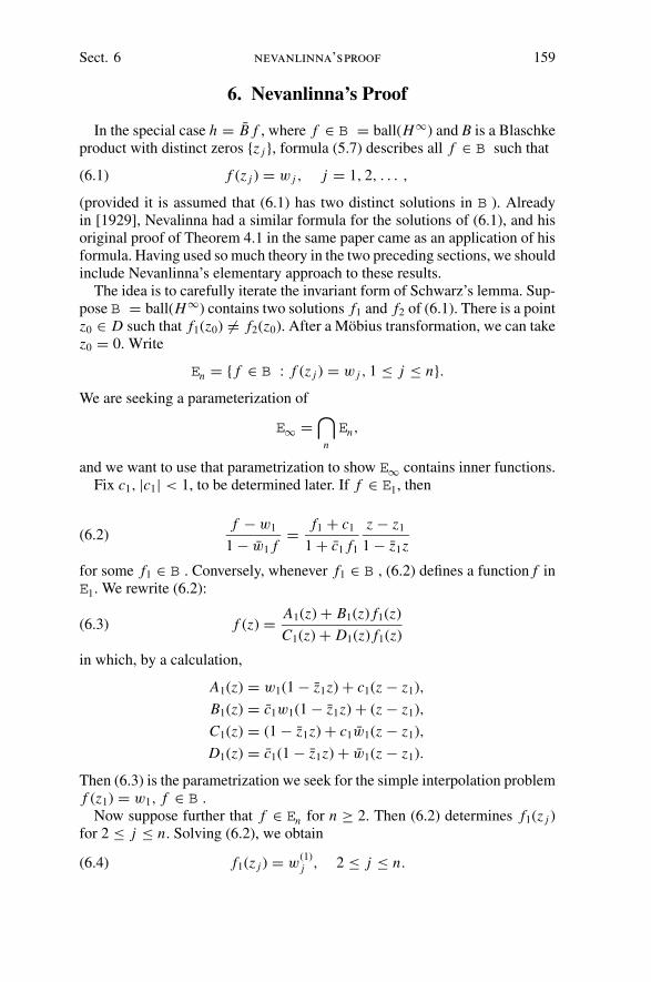
Sect. 6 nevanlinna’sproof 159
6. Nevanlinna’s Proof
In the special case h = B f , where f ∈ B = ball(H∞) and B is a Blaschkeproduct with distinct zeros {z j }, formula (5.7) describes all f ∈ B such that
f (z j ) = w j , j = 1, 2, . . . ,(6.1)
(provided it is assumed that (6.1) has two distinct solutions in B ). Alreadyin [1929], Nevalinna had a similar formula for the solutions of (6.1), and hisoriginal proof of Theorem 4.1 in the same paper came as an application of hisformula. Having used so much theory in the two preceding sections, we shouldinclude Nevanlinna’s elementary approach to these results.
The idea is to carefully iterate the invariant form of Schwarz’s lemma. Sup-pose B = ball(H∞) contains two solutions f1 and f2 of (6.1). There is a pointz0 ∈ D such that f1(z0) �= f2(z0). After a Mobius transformation, we can takez0 = 0. Write
En = { f ∈ B : f (z j ) = w j , 1 ≤ j ≤ n}.We are seeking a parameterization of
E∞ =⋂
n
En,
and we want to use that parametrization to show E∞ contains inner functions.Fix c1, |c1| < 1, to be determined later. If f ∈ E1, then
f − w1
1 − w1 f= f1 + c1
1 + c1 f1
z − z1
1 − z1z(6.2)
for some f1 ∈ B . Conversely, whenever f1 ∈ B , (6.2) defines a function f inE1. We rewrite (6.2):
f (z) = A1(z) + B1(z) f1(z)
C1(z) + D1(z) f1(z)(6.3)
in which, by a calculation,
A1(z) = w1(1 − z1z) + c1(z − z1),
B1(z) = c1w1(1 − z1z) + (z − z1),
C1(z) = (1 − z1z) + c1w1(z − z1),
D1(z) = c1(1 − z1z) + w1(z − z1).
Then (6.3) is the parametrization we seek for the simple interpolation problemf (z1) = w1, f ∈ B .
Now suppose further that f ∈ En for n ≥ 2. Then (6.2) determines f1(z j )for 2 ≤ j ≤ n. Solving (6.2), we obtain
f1(z j ) = w(1)j , 2 ≤ j ≤ n.(6.4)

160 some extremal problems Chap. IV
Clearly |w(1)j | ≤ 1, because f1 ∈ B . Moreover, the case |w(1)
j | = 1 for some
j, 2 ≤ j ≤ n, is not possible, because then f1(z) ≡ w(1)j , |z| < 1, and by (6.2)
En contains exactly one function. Thus we have
|w(1)j | < 1, j = 2, 3, . . . .
Something has been gained, however, because (6.2) allows us to disregard thevalue f1(z1), and En is now described by the n − 1 equations (6.4), instead ofby the original n equations.
Repeating the above reasoning, we fix c2, |c2| < 1, and write
f1 − w(1)2
1 − w(1)2 f1
= f2 + c2
1 + c2 f2
z − z2
1 − z2z.(6.5)
Now f (z) ∈ E2 if and only if f1(z2) = w(1)2 , and that happens if and only if
(6.5) holds for some f2 ∈ B . Furthermore, when n > 2, f ∈ En if and only if
f2(z j ) = w(2)j , 3 ≤ j ≤ n,
where w(2)j is determined by (6.5). We also have |w(2)
j | < 1, for the same reason
that we had |w(1)j | < 1.
Continue by induction, always assumingEn contains more than one function.For k ≤ n, f ∈ En if and only if there are
f0, f1, . . . , fk
in B such that f0 = f , such that
fk(z j ) = w(k)j , k + 1 ≤ j ≤ n,
where |w(k)j | < 1, and w
(0)j = w j , and such that
fk−1 − w(k−1)k
1 − w(k−1)k fk−1
= fk + ck
1 + ck fk
z − zk
1 − zk z,(6.6)
where |ck | < 1, ck to be determined. (The explicit values of the w(k)j are not
important here.)We now iterate (6.6) and obtain a one-to-one mapping of B onto En .
Rewrite (6.6)
fk−1(z) = αk(z) + βk(z) fk(z)
γk(z) + δk(z) fk(z),(6.7)

Sect. 6 nevanlinna’sproof 161
in which
αk(z) = w(k−1)k (1 − zk z) + ck(z − zk),
βk(z) = ckw(k−1)k (1 − zk z) + (z − zk),
γk(z) = (1 − zk z) + ckw(k−1)k (z − zk),
δk(z) = ck(1 − zk z) + w(k−1)k (z − zk).
(6.8)
By induction, (6.3) and (6.7) yield
f (z) = An(z) + Bn(z) fn(z)
Cn(z) + Dn(z) fn(z),(6.9)
in which
An = γn An−1 + αn Bn−1,
Bn = δn An−1 + βn Bn−1,
Cn = γnCn−1 + αn Dn−1,
Dn = δnCn−1 + βn Dn−1
(6.10)
are polynomials of degree at most n in z. Then we have proved
Lemma 6.1. Suppose the polynomials An(z), Bn(z), Cn(z), Dn(z) are definedby (6.8) and (6.10). Then f (z) ∈ En if and only if f (z) satisfies (6.9) for somefn(z) ∈ B .
The polynomials An, Bn, Cn , and Dn depend on the parameters
c1, c2, . . . , cn . Now fix ck = zkw(k−1)k . This makes
δn(0) = Dn(0) = 0
in (6.8) and (6.10), which will facilitate the convergence argument below.When |z| < 1, (6.9) shows that { f (z) : f ∈ En} is a closed disc n(z) con-
tained in D and defined by{
An(z) + Bn(z)ζ
Cn(z) + Dn(z)ζ: |ζ | ≤ 1
}
.(6.11)
When |z| = 1, this formula for n(z) makes sense, although some f ∈ En arenot defined at z. Take n(z) = { f (z) : f ∈ Ao ∩ En}, Ao the disc algebra. Thedisc n(z) degenerates into a point if and only if the determinant
An(z)Dn(z) − Bn(z)Cn(z) = 0.
By (6.10) and induction
(6.12)
An Dn − BnCn = (γnβn − αnδn)(An−1 Dn−1 − Bn−1Cn−1)
=n∏
k=1
(1 − |zk |2|w(k−1)k |2)(1 − |w(k−1)
k |2)(z − zk)(1 − zk z),

162 some extremal problems Chap. IV
where w(0)k = wk . Thus n(z) reduces to a point if and only if z = z j , 1 ≤ j ≤
n. An elementary computation with (6.11) shows that n(z) has radius
ρn(z) = |An Dn − BnCn||Cn|2 − |Dn|2 .
Lemma 6.2. If En �= ∅, then when |z| = 1, n(z) = D, ρn(z) = 1, and
|Bn(z)| = |Cn(z)|,|An(z)| = |Dn(z)|,
An(z)/Cn(z) = (Dn(z)/Bn(z)) = λn(z),
(6.13)
with |λn(z)| < 1.
Proof. The conditions (6.13) follow from the assertion that n(z) = D, bythe well-known characterization of the coefficients of the linear fractionaltransformations
ζ → A + Bζ
C + Dζ
that map D onto itself. That n(z) = D, |z| = 1, is proved by induction. Fixz = eiθ and ζ ∈ D. For n = 1 there exists a constant f1 ∈ B such that
f1(eiθ ) + c1
1 + c1 f1(eiθ )=
(ζ − w1
1 − w1ζ
) / (eiθ − z1
1 − z1eiθ
)
(6.14)
and (6.2) then produces f ∈ E1 such that f (eiθ ) = ζ . For n > 1 the set
{ f1 ∈ B : f1(z j ) = w(1)j , j = 2, . . . , n}
is nonempty, because En �= ∅, and by induction this set contains a functionf1 satisfying (6.14). As before, (6.2) then gives us f ∈ En such that f (eiθ ) =ζ .
Lemma 6.3. Cn(z) has no zeros in |z| ≤ 1.
Proof. If Cn(z) = 0, then by taking ζ = 0 in (6.11), we see that An(z) = 0.Then
An(z)Dn(z) − Bn(z)Cn(z) = 0
and by (6.12), z = z j for some j = 1, 2, . . . , n. Because by (6.12) the deter-minant An Dn − BnCn has only simple zeros, we also have
A′n(z j )Dn(z j ) − Bn(z j )C
′n(z j ) �= 0,
when Cn(z j ) = An(z j ) = 0. Still taking ζ = 0 in (6.11), we then obtain
w j = limz→z j
An(z)/Cn(z) = limz→z j
A′n(z)/C ′
n(Z ).
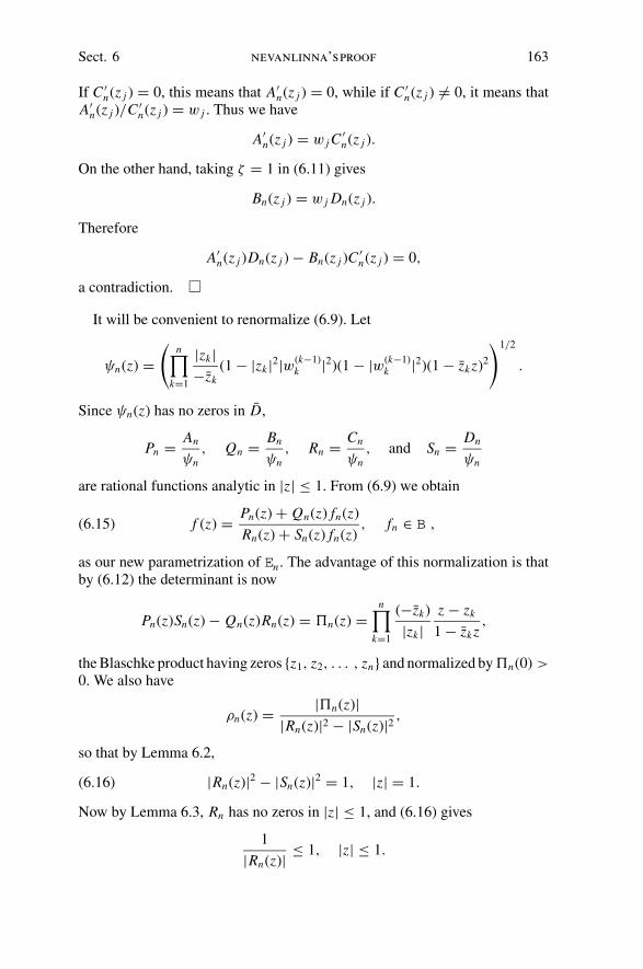
Sect. 6 nevanlinna’sproof 163
If C ′n(z j ) = 0, this means that A′
n(z j ) = 0, while if C ′n(z j ) �= 0, it means that
A′n(z j )/C ′
n(z j ) = w j . Thus we have
A′n(z j ) = w j C
′n(z j ).
On the other hand, taking ζ = 1 in (6.11) gives
Bn(z j ) = w j Dn(z j ).
Therefore
A′n(z j )Dn(z j ) − Bn(z j )C
′n(z j ) = 0,
a contradiction.
It will be convenient to renormalize (6.9). Let
ψn(z) =(
n∏
k=1
|zk |−zk
(1 − |zk |2|w(k−1)k |2)(1 − |w(k−1)
k |2)(1 − zk z)2
)1/2
.
Since ψn(z) has no zeros in D,
Pn = An
ψn, Qn = Bn
ψn, Rn = Cn
ψn, and Sn = Dn
ψn
are rational functions analytic in |z| ≤ 1. From (6.9) we obtain
f (z) = Pn(z) + Qn(z) fn(z)
Rn(z) + Sn(z) fn(z), fn ∈ B ,(6.15)
as our new parametrization of En . The advantage of this normalization is thatby (6.12) the determinant is now
Pn(z)Sn(z) − Qn(z)Rn(z) = �n(z) =n∏
k=1
(−zk)
|zk |z − zk
1 − zk z,
the Blaschke product having zeros {z1, z2, . . . , zn} and normalized by �n(0) >
0. We also have
ρn(z) = |�n(z)||Rn(z)|2 − |Sn(z)|2 ,
so that by Lemma 6.2,
|Rn(z)|2 − |Sn(z)|2 = 1, |z| = 1.(6.16)
Now by Lemma 6.3, Rn has no zeros in |z| ≤ 1, and (6.16) gives
1
|Rn(z)| ≤ 1, |z| ≤ 1.
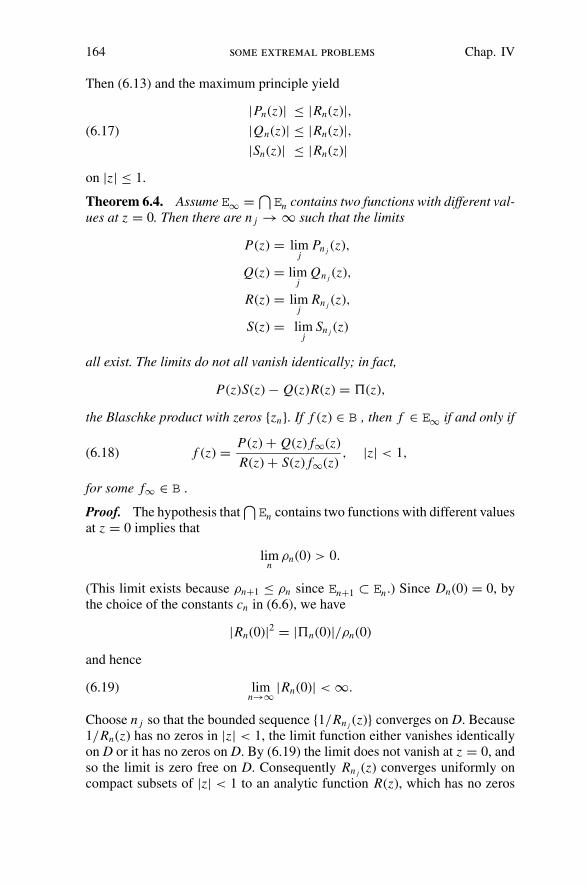
164 some extremal problems Chap. IV
Then (6.13) and the maximum principle yield
|Pn(z)| ≤ |Rn(z)|,|Qn(z)| ≤ |Rn(z)|,|Sn(z)| ≤ |Rn(z)|
(6.17)
on |z| ≤ 1.
Theorem 6.4. Assume E∞ = ⋂En contains two functions with different val-
ues at z = 0. Then there are n j → ∞ such that the limits
P(z) = limj
Pn j (z),
Q(z) = limj
Qn j (z),
R(z) = limj
Rn j (z),
S(z) = limj
Sn j (z)
all exist. The limits do not all vanish identically; in fact,
P(z)S(z) − Q(z)R(z) = �(z),
the Blaschke product with zeros {zn}. If f (z) ∈ B , then f ∈ E∞ if and only if
f (z) = P(z) + Q(z) f∞(z)
R(z) + S(z) f∞(z), |z| < 1,(6.18)
for some f∞ ∈ B .
Proof. The hypothesis that⋂En contains two functions with different values
at z = 0 implies that
limn
ρn(0) > 0.
(This limit exists because ρn+1 ≤ ρn since En+1 ⊂ En .) Since Dn(0) = 0, bythe choice of the constants cn in (6.6), we have
|Rn(0)|2 = |�n(0)|/ρn(0)
and hence
limn→∞ |Rn(0)| < ∞.(6.19)
Choose n j so that the bounded sequence {1/Rn j (z)} converges on D. Because1/Rn(z) has no zeros in |z| < 1, the limit function either vanishes identicallyon D or it has no zeros on D. By (6.19) the limit does not vanish at z = 0, andso the limit is zero free on D. Consequently Rn j (z) converges uniformly oncompact subsets of |z| < 1 to an analytic function R(z), which has no zeros

Sect. 6 nevanlinna’sproof 165
on |z| < 1. By (6.17) we can take a finer subsequence {n j } so that
limj
Pn j (z) = P(z),
limj
Qn j (z) = Q(z),
and
limj
Sn j (z) = S(z)
also all exist. Then
P(z)S(z) − Q(z)R(z) = limj
�n j (z) = �(z),
and so the limit functions are not all identically zero.If f ∈ ⋂
En , then by Lemma 6.1 there is fn ∈ B such that
f = Pn + Qn fn
Rn + Sn fn.
Refine the subsequence {n j } so that fn j (z) → f∞(z), |z| < 1, with f∞ ∈ B .Then (6.18) follows. Conversely, if f∞ ∈ B , then
f (n) = Pn + Qn f∞Rn + Sn f∞
.
is in En , and f (n j ) has limit f ∈ E∞.
It turns out that P, Q, R, and S do not depend on the subsequence {n j }.They are uniquely determined by the original interpolation problem (6.1) andby the choice of the constants cn in (6.6). We shall not make use of this fact,however.
Before turning to Nevanlinna’s proof that E∞ contains inner functions,we mention a simple consequence of (6.18). Because En+1 ⊂ En , the discsn(z), |z| < 1, decrease to a limit disc ∞(z) = { f (z) : f ∈ E∞}. By (6.18),
∞(z) ={
P(z) + Q(z)ζ
R(z) + S(z)ζ: |ζ | < 1
}
.
Since the determinant of the coefficients for this mapping is P(z)S(z) −Q(z)R(z) = �(z), ∞(z) is nontrivial whenever z �∈ {z j }. The radius of∞(z)is
ρ∞(z) = limn
ρn(z) = �(z)
|R(z)2| − |S(z)|2 .
Returning to n(z0), |z0| < 1, and to its parametrization (6.11), we see thatf ∈ En solves the extremal problem f (z0) ∈ ∂n(z0) if and only if
f (z) = An(z) + Bn(z)eiϕ
Cn(z) + Dn(z)eiϕ= Pn(z) + Qn(z)eiϕ
Rn(z) + Sn(z)eiϕ

166 some extremal problems Chap. IV
for some unimodular constant eiϕ . Thus f (z) is a rational function of degreeat most n. On two other occasions (Corollary 1.9 of this chapter and Corol-lary 2.4, Chapter I), we have seen that the extremal function f (z) is a finiteBlaschke product. This fact also follows from the reasoning in this section,because by Lemma 6.2, | f (z)| = 1 for |z| = 1. Further analysis of the poly-nomials An(z), Bn(z), Cn(z), and Dn(z) shows that the Blaschke product f (z)has degree n. (See Exercise 20.)
The preceding discussion suggests that we might find an inner functionin E∞ by setting f∞ = eiϕ in (6.18). That is how Nevanlinna first provedTheorem 4.1. The proof above of Theorem 4.4 was based on the same idea: Theunimodular function h0 ∈ K was obtained by maximizing the linear functionalRe
∫h dθ/2π, h ∈ K .
We return to Theorem 4.1, which we restate as follows.
Theorem 6.5. If E∞ contains two distinct functions, and if eiϕ is any uni-modular constant, then
f (z) = P(z) + Q(z)eiϕ
R(z) + S(z)eiϕ(6.20)
is an inner function in E∞.
Proof. By Theorem 6.4, f ∈ E∞, and in particular ‖ f ‖∞ ≤ 1. We supposethere exists E ⊂ T, |E | ≡ ∫
χE (θ )dθ/2π > 0, such that
| f (eiθ )| ≤ α < 1, θ ∈ E,(6.21)
and we argue toward a contradiction.Reindex so that Rn(z) → R(z), Pn(z) → P(z), Qn(z) → Q(z), and
Sn(z) → S(z). Fix M > |R(0)|. Since by Lemma 6.3 Rn(z) has no zeros onD, we have
log M > log |Rn(0)| = 1
2π
∫log |Rn(eiθ )|dθ
for large n, say n > n0. By (6.16), log |Rn(eiθ )| ≥ 0, and hence
|{θ : log |Rn(eiθ )| > 2 log M/|E |}| ≤ |E |/2,
n > n0. Therefore
En = {θ ∈ E : |Rn(eiθ )| ≤ M2/|E |}satisfies
|En| ≥ |E |/2, n > n0.
By (6.16) and (6.13), we also have
∣∣∣∣
Pn(eiθ )
Rn(eiθ )
∣∣∣∣
2
= 1 − 1
|Rn(eiθ )|2 ,

Sect. 6 nevanlinna’sproof 167
which gives∣∣∣∣
Pn(eiθ )
Rn(eiθ )
∣∣∣∣ ≤ {1 − M−4/|E |}1/2 = β < 1,(6.22)
for θ ∈ En, n > n0.Because f ∈ En there exists fn ∈ B such that
f (z) = Pn(z) + Qn(z) fn(z)
Rn(z) + Sn(z) fn(z).
Since the rational functions Pn, Qn, Rn , and Sn are continuous on D and since|Pn Sn − Qn Rn| = 1 on T, fn(z) has radial limit fn(eiθ ) whenever f (z) hasradial limit f (eiθ ). Thus at eiθ ∈ E, fk(eiθ ) exists and
f (eiθ ) = Pn(eiθ ) + Qn(eiθ ) fn(eiθ )
Rn(eiθ ) + Sn(eiθ ) fn(eiθ ).
By Lemma 6.2, the mapping
ζ → Pn(eiθ ) + Qn(eiθ )ζ
Rn(eiθ ) + Sn(eiθ )ζ,
which is an automorphism of D, preserves the pseudohyperbolic distance.Hence
| fn(eiθ )| = ρ( fn(eiθ ), 0) = ρ( f (eiθ ), Pn(eiθ )/Qn(eiθ )).
For n > n0 and for eiθ ∈ En , (6.21) and (6.22) then yield
| fn(eiθ )| ≤ | f (eiθ )| + |Pn(eiθ )|/|Rn(eiθ )|1 + | f (eiθ )||Pn(eiθ )|/|Rn(eiθ )|
≤ α + β
1 + αβ= γ < 1.
Consequently
| fn(0)| ≤ 1
2π
∫| fn(eiθ )|dθ ≤ (γ |En| + (1 − |En|))
≤{
γ|E |2
+(
1 − |E |2
)}
= η < 1.
Take a subsequence { fn j } so that fn j (0) → ζ, |ζ | ≤ η < 1. Then
f (0) = limj
Pn j (0) + Qn j (0) fn j (0)
Rn j (0) + Sn j (0) fn j (0)= P(0) + Q(0)ζ
R(0) + S(0)ζ.
Since P(0)S(0) − Q(0)R(0) �= 0, we conclude from (6.20) that ζ = eiϕ, acontradiction.
An interesting apparently unsolved problem is to determine whether or whenE∞ contains a Blaschke product. See page vii.

168 some extremal problems Chap. IV
Notes
The first systematic treatment of dual extremal problems is the pa-per of Macintyre and Rogosinski [1950]. The functional analytic methodswere introduced by Havinson [1949,1951] and by Rogosinski and Shapiro[1953]. Duren’s book [1970] contains a slightly different treatment andsome references to the older literature. See also Goluzin [1952] and Landau[1916].
Section 2 is from the paper of Carleson and Jacobs [1972]. Kahane[1974] discusses a number of related questions. An interesting open prob-lem is to find intrinsic necessary and sufficient conditions for a function inL∞ to have unique best approximation in H∞. Exercise 17 gives a partialanswer.
The primary references for Section 3 are Szego [1920] and Helson andSzego [1960]. Exercises 8 and 14 outline results similar to the Helson–Szegotheorem.
Most of the material in Sections 4 and 5 originates with Adamyan, Arov,and Krein [1968], but the proofs in the text are considerably different fromtheir spectral theory approach. In [1971] Adamyan, Arov, and Krein extendtheir results to the matrix valued case. Theorem 5.1 and Theorem 5.2 are fromdeLeeuw and Rudin [1958].
Section 6 is from Nevanlinna’s paper [1929], which includes a number ofother classical results, all derived ultimately from Schwarz’s lemma. It is afundamental paper long overlooked. Schur’s [1917] treatment of the coefficientproblem is very similar. It is outlined in Exercise 21.
Exercises and Further Results
1. If f ∈ L p(�), 1 ≤ p ≤ ∞, then
infg∈H p
‖ f − g‖p = supG∈Hq
‖G‖q=1
∣∣∣∣
∫f G dx
∣∣∣∣ .
2. Let f (z) be meromorphic on |z| < 1, and suppose that on someannulus R < |z| < 1, f (z) is analytic and of class H 1 (i.e. | f (z)| possesses aharmonic majorant). Then f (eiθ ) exists almost everywhere. Prove f (eiθ ) ≥ 0almost everywhere if and only if f (z) is a rational function of the form
cn∏
j=1
(z − α j )(1 − α j z)
/n∏
j=1
(z − β j )(1 − β j z),
where |α j | ≤ 1, |β j | ≤ 1, c > 0.
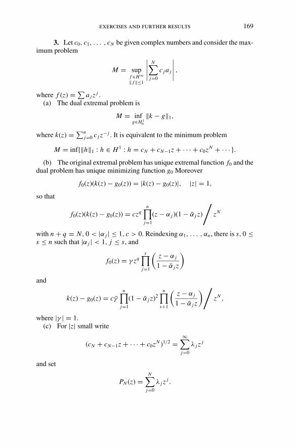
exercises and further results 169
3. Let c0, c1, . . . , cN be given complex numbers and consider the max-imum problem
M = supf ∈H∞‖ f ‖≤1
∣∣∣∣∣
N∑
j=0
c j a j
∣∣∣∣∣,
where f (z) = ∑a j z j .
(a) The dual extremal problem is
M = infg∈H 1
0
‖k − g‖1,
where k(z) = ∑nj=0 c j z− j . It is equivalent to the minimum problem
M = inf{‖h‖1 : h ∈ H 1 : h = cN + cN−1z + · · · + c0zN + · · · }.(b) The original extremal problem has unique extremal function f0 and the
dual problem has unique minimizing function g0 Moreover
f0(z)(k(z) − g0(z)) = |k(z) − g0(z)|, |z| = 1,
so that
f0(z)(k(z) − g0(z)) = czqn∏
j=1
(z − α j )(1 − α j z)
/
zN
with n + q = N , 0 < |α j | ≤ 1, c > 0. Reindexing α1, . . . , αn , there is s, 0 ≤s ≤ n such that |α j | < 1, j ≤ s, and
f0(z) = γ zqs∏
j=1
(z − α j
1 − α j z
)
and
k(z) − g0(z) = cγn∏
j=1
(1 − α j z)2n∏
s+1
(z − α j
1 − α j z
)/
zN ,
where |γ | = 1.(c) For |z| small write
(cN + cN−1z + · · · + c0zN )1/2 =∞∑
j=0
λ j zj
and set
PN (z) =N∑
j=0
λ j zj .
170 some extremal problems Chap. IV
Assume PN (z) has no zeros in |z| < 1. Then there exist α1, . . . , αn, n ≤ N ,
such that 0 < |α j | ≤ 1 and such that
PN (z) = λ0
n∏
j=1
(1 − α j z).
Then
z−N P2N = cN z−N
n∏
j=1
(1 − α j z)2
has the form k − g, g ∈ H 1. Setting
f0(z) = cN
|cN | zN−nn∏
j=1
(z − α j
1 − α j z
)
,
we obtain f0 P2N /zN ≥ 0 on |z| = 1. Consequently f0 is the extremal function,
k(z) − g0(z) = P2N (z)/zN , and
M = ‖P2N ‖1 =
N∑
j=0
|λ j |2.
(d) Landau [1913, 1916] determined the extremum M in the special casec j = 1 by a different method. In this case PN = �N
0 λ j z j , where
λ j = (−1) j
(− 12
j
)
= (2 j )!
4 j ( j!)2,
and by Wallis’s formula
M ∼ log N/π (N → ∞).
Thus M has the same order of magnitude as the Lebesgue constants ‖DN ‖1,
where DN = �N−N ei jθ is Dirichlet’s kernel for partial sums.
The dual problem in part (a) was first treated by F. Riesz [1920] using avariational argument.
4. A function f ∈ C(T ) is called badly approximable if its nearestfunction g in H∞ satisfies g ≡ 0. Show f is badly approximable if and onlyif | f (eiθ )| is a positive constant and f (eiθ ) has negative winding number (seePoreda [1972] or Gamelin, Garnett, Rubel, and Shields [1976]).
5. Let g ∈ H∞ be the best approximation to f ∈ C(T ). It conjecturedthat g is continuous if the conjugate function f is continuous. (See page vii.)The converse of this is false. Use Exercise 4 above to find a badly approx-imable function whose conjugate function is not continuous (D. Sarason, un-published).
exercises and further results 171
6. Let f ∈ C(T ), f �∈ H∞, let g ∈ H∞ be the best approximation to f,and let F ∈ H 1
0 be a dual extremal function, so that
( f − g)F = ‖ f − g‖∞|F |almost everywhere.
(a) F can be chosen so that F(z)/z is outer.(b) If F1 ∈ H 1
0 is another dual extremal function, then F/F1 is a rationalfunction.
(c) F is unique if and only if z/F ∈ H 1. In that case z/F ∈ H p for allp < ∞.
(d) More generally, if f ∈ L∞\H∞, if F exists, and if z/F ∈ H 1, then Fis unique.
(See deLeeuw and Rudin [1958] and Carleson and Jacobs [1972].)
7. If f ∈ H∞, then
dist( f, Ao) ≤ 2 dist( f, C(T )),
where Ao = H∞ ∩ C(T ) is the disc algebra. The constant 2 is sharp. (SeeDavie, Gamelin, and Garnett [1973].)
�8. Let dμ = w dθ/2π + dμs be a positive measure on the circle. Then
inff ∈F
∫|1 − Re f |2dμ =
(∫w−1 dθ
2π
)−1
,
where F is the set of trigonometric polynomials �n>0 aneinθ (see Grenanderand Rosenblatt [1957]). The result is due to Kolmogoroff [1941].
9. Find two closed subspaces F and G of a Hilbert space such that
F ∩ G = {0}but such that
1 = sup{|〈 f, g〉| : f ∈ F , g ∈ G, ‖ f ‖ = ‖g‖ = 1}.
10. If F and G are subspaces of L2(μ), then ρ = 1 if and only if
0 = inf
{∫| f − g|2dμ : f ∈ F , g ∈ G; ‖ f ‖ ≥ 1, ‖g‖ ≥ 1
}
.
Hence the property ρ = 1 is unchanged if dμ is replaced by w dμ, w boundedabove and below.
11. If a weight function w satisfies the Helson–Szego condition (3.3),then for some ε > 0, w ∈ L1+ε and w−1 ∈ L1+ε.
12. Let w be a weight function. Assumeψ = (log w) is continuous exceptfor jumps at a finite number of points. Then w satisfies (3.3) if and only if eachjump is less than π (Helson and Szego [1960]).

172 some extremal problems Chap. IV
13. Let α be real. There is a constant Kα such that∫ π
−π
| p(θ )|2|θ |αdθ ≤ Kα
∫ π
−π
|p(θ )|2|θ |αdθ
for all trigonometric polynomials if and only if −1 < α < 1 (see Hardy andLittlewood [1936]).
��14. Let F n be the set of all trigonometric polynomials �k≥nakeikθ and
let Gn = F n be the set of trigonometric polynomials of the form �k≥nbke−ikθ .When μ is a positive finite measure on T write
ρn = sup
∣∣∣∣
∫f g dμ
∣∣∣∣ ,
where f ∈ F n, g ∈ Gn,∫ | f |2dμ ≤ 1, and
∫ |g|2dμ ≤ 1. Wright
dμ = w dθ/2π + dμs
with dμs, singular to dθ .(a) If dμs �= 0 or if log w /∈ L1, then ρn = 1 for all n.(b) Now assume dμ = w dθ/2π with
ϕ = log w ∈ L1.
Let W be the set of weights w such that
limn→∞ ρn = 0,
where dμ = w dθ/2π . Then w ∈ W if and only if e−i ϕ ∈ H∞ + C .(c) H∞ + C is a closed subalgebra of L∞.(d) Let W0 be the set of positive weights w such that, for every ε > 0,
ϕ = log w = r + s + t
with ‖r‖∞ < ε, ‖s‖∞ < ε, and t ∈ C . Then W0 ⊂ W and w ∈ W if and only ifw = |p|2w0, where w0 ∈ W0 and p is a trigonometric polynomial. (The set logW0 is the space VMO to be studied in Chapter VI.) (See Helson and Sarason[1967].)
15. Let u be a unimodular function in L∞ and set
S u = {G ∈ H 1 : ‖G‖1 = 1, G/|G| = u}.(a) There exist functions u for which S u = ∅.(b) If F ∈ S u , and if 1/F ∈ H 1, then S u = {F}.(c) If F ∈ S u = {F}, then for all α, |α| = 1, (z − α)−2 F(z) /∈ H 1. (See
deLeeuw and Rudin [1958].)
16. Let h ∈ L∞, |h| = 1 almost everywhere.(a) If dist(h, H∞) < 1, then h = F/|F | for some F ∈ H 1. Moreover, the
outer factor of F is invertible in H 1. (See Lemma 5.4.)
exercises and further results 173
(b) If dist(h, H∞) < 1 but dist (h, H∞0 ) = 1, then h = F/|F | for some
F ∈ H 1. (See Case 1 of the proof of Theorem 4.4.) It follows thatdist(h, H∞) < 1.
17. (a) Let h ∈ L∞. If the coset h + H∞ is an extreme point of ball(L∞/H∞) then there is g ∈ H∞ such that |h + g| = 1 almost everywhere.
(b) Now suppose |h| = 1 almost everywhere. Then h + H∞ is an extremepoint of ball(L∞/H∞) if and only if ‖h + g‖ > 1 for all g ∈ H∞, g �= 0.Thus the extreme points of ball(L∞/h∞) are the cosets containing exactly onefunction of unit modulus (see Koosis [1971]).
(c) If |h| = 1 almost everywhere, then ‖h + g‖∞ > 1 for all g ∈ H∞, g �=0, if and only if h cannot be written as F/|F |, F ∈ H 1. (See Lemmas 5.4and 5.5.) This is a weak generalization of Exercise 5. If |h| = 1, then h isbadly approximable by H∞(‖h − g‖ > 1 if g ∈ H∞, g �= 0) if and only if his not the argument of an H 1 function. Example 4.2 shows there exist badlyapproximable functions not having constant modulus.
(d) L∞/H∞ is a dual space. Hence ball(L∞/H∞) is the weak-star closedconvex hull of the set of cosets {h + H∞ : |h| = 1, h badly approximable}.
18. Let F ∈ H 1, ‖F‖1 = 1. Then every g ∈ H∞ such that
‖F/|F | − g‖∞ ≤ 1
is of the form (5.10) if and only if S F/|F | = {F}.19. Let f ∈ H∞, ‖ f ‖∞ = 1. Then f is an extreme point of ball(H∞)
if and only if
∫log(1 − | f (eiθ )|)dθ = −∞
(see deLeeuw and Rudin [1958]).
20. In the notation of Section 6, and with ck = zkw(k−1)k , An(z) has degree
at most n − 1 and Bn(z) has degree n. When eiϕ is a unimodular constant, thepolynomials An(z) + Bn(z)eiϕ and Cn(z) + Dn(z)eiϕ have no common zero.Thus
f (z) = An(z) + Bn(z)eiϕ
Cn(z) + Dn(z)eiϕ
is a Blaschke product of degree n.
�21. Fix complex numbers c0, c1, . . . and set
En = { f ∈ B : f (z) = c0 + c1z + · · · + cnzn + · · · }.
Write γ0 = c0 and assume |γ0| ≤ 1.

174 some extremal problems Chap. IV
(a) If |γ0| = 1 then E0 contains exactly one function, f = γ0. Suppose|γ0| < 1 and write f ∈ E0
f = z f1 + γ0
1 + γ0z f1
,(E.1)
with f1 ∈ B . So E0 is in one-to-one correspondence with B . Then f ∈ E1 ifand only if f1(0) = γ1 = c1/(1 − |c0|2). In particular E1 �= ∅ if and only if|γ1| ≤ 1, and E1 consists of exactly one function if and only if |γ1| = 1.
(b) Continue by induction. We obtain γ0, γ1, . . . , γn, . . . . If |γ0| <
1, |γ1| < 1, . . . , |γn| < 1, then En is in one-to-one correspondence with Bthrough the formulas f0 = f ,
fk−1 = z fk + γk−1
1 + γk−1z fk, 1 ≤ k ≤ n,
fk ∈ β. If |γk | = 1 but |γ j | < 1, j < k, then Ek consists of exactly one func-tion, a Blaschke product of degree k.
(c) Suppose En �= ∅. Then the (n + 1)th coefficients cn+1 of the functionsin En fill a closed disc with radius
ωn = (1 − |γ0|) · · · (1 − |γn|).(E.2)
(Use (E.1) and induction.)(d) Suppose
⋂En �= ∅. Then of course
⋂En = { f }, f = �∞
0 cnzn . Prove
limn→∞ ωn = exp
1
2π
∫log(1 − | f |2) dθ.
(Hint: By (E.1) and (E.2) we have, on |z| = 1,
1 − | f |2 = (1 − |γ0|2)(1 − | f1|2)
|1 + γ0 f1|2 = ωn(1 − | fn+1|2)∏n
j=0 |1 + γ j z f j+1|2 .
Because the denominator has no zeros on D, this gives
exp1
2π
∫log(1 − | f |2)dθ = ωn exp
1
2π
∫log(1 − | fn+1|2)dθ ≤ ωn.
For the reverse inequality use Szegos theorem. For ε > 0 there is P(z) =1 + b1z + · · · + bN zN such that
∫|P|2(1 − | f |2)
dθ
2π≤ ε + exp
1
2π
∫log(1 − | f |2)dθ.
Let f ∗ ∈ En be obtained by setting fn+1 = 0. Then by Szegos theorem
ωn = exp
∫log(1 − | f ∗|2)
dθ
2π≤
∫|P|2(1 − | f |∗2)
dθ
2π.
exercises and further results 175
By the Parseval relation,
limn→∞
∫|P|2(1 − | f ∗|2)
dθ
2π≤
∫|P|2(1 − | f |2)
dθ
2π.
(e) Let An be the matrix⎡
⎢⎢⎣
c0 c1 · · · cn
0 c0 cn−1
......
0 · · · 0 c0
⎤
⎥⎥⎦
and let In be the (n + 1) × (n + 1) identity matrix. Then En �= ∅ if and only ifIn − A∗
n An is nonnegative definite. If In − A∗n An is positive definite, then En
is infinite. More precisely,
det(In − A∗n An) = ω0 ω1 · · · ωn.
(See Schur [1917], except for part (d), which is due to Boyd [1979].)
V
Some Uniform Algebra
This chapter develops the background from uniform algebra theory whichwill be needed for our analysis of H∞ below. Our treatment is quite brief. Fora complete picture of the general theory the reader is referred to the books ofBrowder [1969], Gamelin [1969], and Stout [1971].
However, two topics special to H∞ will be covered in detail. In Section2 we prove Marshall’s theorem that the Blaschke products generate H∞. InSection 5, three theorems on the predual of H∞ are proved by representinglinear functionals as measures on the Silov boundary of H∞.
1. Maximal Ideal Spaces
A Banach algebra is a complex algebra A which is also a Banach spaceunder a norm satisfying
‖ f g‖ ≤ ‖ f ‖ ‖g‖, f, g ∈ A.(1.1)
We always assume that A is commutative ( f g = g f, f, g ∈ A) and that there isa unit 1 ∈ A(1 · f = f, f ∈ A). The correspondence λ → λ · 1 identifies thecomplex field � as a subalgebra of A. We say f ∈ A is invertible if there isg ∈ A such that g f = 1. The unique inverse is denoted by g = f −1. Write
A−1 = { f ∈ A : f −1 exists}for the set of invertible elements of A. A complex homomorphism, or multi-plicative linear functional, is a nonzero homomorphism m : A → � from Ainto the complex numbers. Trivially m(1) = 1.
Theorem 1.1. Every complex homomorphism of A is a continuous linearfunctional with norm at most one,
‖m‖ = sup‖ f ‖≤1
|m( f )| ≤ 1.
176
Sect. 1 maximal ideal spaces 177
Proof. Because m is linear, we only have to prove that ‖m‖ ≤ 1. If m isunbounded, or if ‖m‖ > 1, then there is f ∈ A such that ‖ f ‖ < 1 but suchthat m( f ) = 1. By (1.1) the series
∞∑
n=0
f n
is norm convergent. Its sum satisfies
(1 − f )∞∑
n=0
f n = 1,(1.2)
so that 1 − f ∈ A−1. But then
1 = m(1) = m((1 − f )−1)(m(1) − m( f )) = 0,
a contradiction.
Theorem 1.2. Suppose M is a maximal ( proper) ideal in A. Then M is thekernel of a complex homomorphism m : A → �.
Proof. There are two steps. First we show M is closed. Now, if the closureM of M is proper, that is, if M �= A, then M is also an ideal in A. Therefore Mis closed if M �= A, because M is maximal. However, if g ∈ M , then g �∈ A−1
and (1.2), applied to f = 1 − g, shows that ‖1 − g‖ ≥ 1. Hence 1 �∈ M andM is closed.
The second step is to show the quotient algebra B = A/M satisfies
B = � · 1,
where 1 = 1 + M now denotes the unit in B. The quotient mapping will thendefine the complex homomorphism with kernel M. Since M is maximal, B =A/M is a field, and since M is closed, B is complete in the quotient norm
‖ f + M‖ = infg∈M
‖ f + g‖,
which also satisfies (1.1).Suppose there exists f ∈ B\� · 1. Then f − λ ∈ B−1 for all λ ∈ �, because
B is a field. On the disc |λ − λ0| < 1/‖( f − λ0)−1‖, the series
∞∑
n=0
(λ − λ0)n(( f − λ0)−1)n+1(1.3)
converges in norm to ( f − λ)−1, because of the identity
1
f − λ= 1
( f − λ0)
1
[1 − (λ − λ0)/( f − λ0)].
178 some uniform algebra Chap. V
Clearly f −1 �= 0, and by the Hahn–Banach theorem there is a bounded linearfunctional L on B such that ‖L‖ = 1 and
L( f −1) �= 0.(1.4)
Since (1.3) is norm convergent and since ‖L‖ = 1, we have
F(λ) = L(( f − λ)−1) =∞∑
n=0
L((( f − λ0)−1)n+1)(λ − λ0)n,
when |λ − λ0| < 1/‖( f − λ0)−1‖. Becauseλ0 is arbitrary, this means that F(λ)is an entire analytic function. Now for |λ| large, (1.2) yields
‖( f − λ)−1‖ = 1
|λ|
∥∥∥∥∥
(
1 − f
λ
)−1∥∥∥∥∥
≤ 1
|λ|∞∑
n=0
‖ f ‖n
|λ|n .
Consequently,
|F(λ)| = |L(( f − λ)−1)| ≤ C/|λ|, |λ| large,
and by Liouville’s theorem F ≡ 0. Hence
L( f −1) = F(0) = 0,
contradicting (1.4).
The set MA of complex homomorphisms of A is called the spectrum ormaximal ideal space of A. By Theorem 1.1, MA is contained in the unit ballof the dual Banach space A∗. Give MA the weak-star topology of A∗, inwhich a basic neighborhood V of m0 ∈ MA is determined by ε > 0 and byf1, f2, . . . , fn ∈ A:
V = {m ∈ MA : |m( f j ) − m0( f j )| < ε, 1 ≤ j ≤ n}.This topology onMA is called the Gelfand topology. With the Gelfand topologyMA is a weak-star closed subset of ball(A∗), because
MA = {m ∈ ball(A∗) : m( f g) = m( f )m(g), f, g ∈ A}.By the Banach–Alaoglu theorem, which says ball(A∗) is weak-star compact,MA is a compact Hausdorff space. Writing
f (m) = m( f ), f ∈ A, m ∈ MA,
we have a homomorphism f → f from A into C(MA), the algebra of con-tinuous complex functions on MA. This homomorphism is called the Gelfandtransform. By Theorem 1.1, the Gelfand transfrom is norm decreasing:
‖ f ‖ = supm∈MA
| f (m)| ≤ ‖ f ‖.

Sect. 1 maximal ideal spaces 179
By Theorem 1.2, f ∈ A−1 if and only if f (m) is nowhere zero. Indeed, if f �∈A−1, then by Zorn’s lemma the ideal { f g : g ∈ A} is contained in a (proper)maximal ideal.
The Banach algebra A is called a uniform algebra if the Gelfand transformis an isometry, that is, if
‖ f ‖ = ‖ f ‖, f ∈ A.
Theorem 1.3. The Gelfand transform is an isometry if and only if
‖ f 2‖ = ‖ f ‖2(1.5)
for all f ∈ A.
Proof. Since ‖ f ‖ is a supremum, ‖ f 2‖ = ‖ f ‖2 and (1.5) holds for any uni-form algebra.
Now assume (1.5). By Theorem 1.1, we have ‖ f ‖ ≤ ‖ f ‖. To completethe proof we take f ∈ A with ‖ f ‖ = 1, we fix ε > 0, and we show ‖ f ‖ ≤1 + ε. By Theorem 1.2, f − λ ∈ A−1 when |λ| > 1 = ‖ f ‖. By (1.3) the A-valued function ( f − λ)−1 is analytic on |λ| > 1. This means that wheneverL ∈ A∗, the scalar function F(λ) = L(( f − λ)−1) is analytic on |λ| > 1. Bycompactness,
sup|λ|=1+ε
‖( f − λ)−1‖ = K
is finite. By (1.2),
F(λ) = L
(−1
λ
(
1 − f
λ
)−1)
= −∞∑
n=0
L( f n)
λn+1, |λ| > ‖ f ‖.
This series must also represent F(λ) on |λ| > 1. Taking ‖L‖ = 1 we obtainfrom Cauchy’s theorem,
L( f n) =∣∣∣∣−
1
2π i
∫
|λ|=1+ε
F(λ)λndλ
∣∣∣∣ ≤ (1 + ε)n+1 K .
Consequently, by the Hahn–Banach theorem,
‖ f n‖ = sup‖L‖=1
|L( f n)| ≤ (1 + ε)n+1 K .
Setting n = 2k and using (1.5), we conclude that
‖ f ‖ ≤ limk→∞
(K (1 + ε)2k+1)1/2k = 1 + ε,
as desired.
When A is a uniform algebra, the range A of the Gelfand transform is auniformly closed subalgebra of C(MA), and A is isometrically isomorphic to

180 some uniform algebra Chap. V
A. In that case we identify f with f and write
f (m) = m( f ) = f (m), f ∈ A, m ∈ M.
Thus we view A as a uniformly closed algebra of continuous functions onMA. Note that A separates the points of MA and that A contains the constantfunctions on MA.
Example 1. Suppose A is any algebra of continuous complex functions on acompact Hausdorff space Y. If A has the uniform norm, ‖ f ‖ = supy∈Y | f (y)|and if A is complete, then A is a uniform algebra. If A contains the constantfunctions and separates the points of Y, then Y is homeomorphic to a closedsubset of MA, and we say that A is a uniform algebra on Y. This is the genericexample, because any uniform algebra A is clearly a uniform algebra on itsspectrum Y = MA. If A = C(Y ), then MA = Y . (See Exercise 5.)
Example 2. Let l∞ denote the space of bounded complex sequences. With thenorm ‖x‖ = supn |xn| and with the pointwise multiplication (xy)n = xn yn, l∞is a uniform algebra, by Theorem 1.3. The maximal ideal space of l∞ has thespecial name β�, the Stone–Cech compactification of the positive integers�.
The Gelfand transform of l∞ is C(β�). To see this, note that if x ∈ l∞ isreal, that is, if xn ∈ � for all n, then x(m) is real on Ml∞ = β�, because then(x − λ)−1 ∈ l∞ whenever Im λ �= 0. It now follows from the Stone–Weier-strass theorem that l∞ = C(β�).
Since the functional mn(x) = xn is multiplicative on l∞, � can be identifiedwith a subset of β�, and the Gelfand topology is defined in such a way that� is homeomorphic to its image in β�. Moreover, � is dense in β�, becauseevery function in C(β�) = l∞ is completely determined by its behavior on �.
The Stone–Cech compactification β� can also be characterized functorially.
Theorem 1.4. Let Y be a compact Hausdorff space and let τ : � → Y be acontinuous mapping. Then the mapping τ has a unique continuous extensionτ : β� → Y .
If τ (�) is dense in Y and if the images of disjoint subsets of � have disjointclosures in Y, then the extension τ is a homeomorphism of β� onto Y.
Proof. The mapping
T : C(Y ) → l∞,
defined by T f (n) = f ◦ τ (n), is a homomorphism from C(Y ) into l∞. BecauseT is continuous, the adjoint mapping T ∗ : (l∞)∗ → (C(Y ))∗ is weak-star toweak-star continuous. If m ∈ (l∞)∗ is a multiplicative linear functional, thatis, if m ∈ β�, then since T ( f g) = T ( f )T (g), T ∗(m) is also a multiplicativelinear functional on C(Y ), and by Exercise 5, T ∗(m) ∈ Y = MC(Y ). RestrictingT ∗ to β�, we have a mapping τ (m) = T ∗(m) from β� into Y, and by thedefinition of T, τ (n) = τ (n), n ∈ �. Since β� has the weak-star topology of

Sect. 1 maximal ideal spaces 181
(l∞)∗ and Y = MC(Y ) has the weak-star topology of (C(Y ))∗, the mapping τ
is continuous. Because � is dense in β�, τ is the unique continuous extensionof τ to β�.
Now suppose that τ (S1) ∩ τ (S2) = ∅ wherever S1 ⊂ �, S2 ⊂ � and S1 ∩S2 = ∅. Then there is f ∈ C(Y ) such that f = 1 on τ (S1) and f = 0 on τ (S2).We can assume that S2 = �\S1, so that T f = χS1
. Because linear combinationsof characteristic functions are dense in l∞, this means the range of T is densein l∞. If we further assume that τ (�) is dense in Y, then we have ‖T f ‖ =‖ f ‖, f ∈ C(Y ), and the mapping T is an isometry. Consequently the range ofT is norm closed in l∞. Hence the range of T is both dense and closed and Tmaps C(Y ) onto l∞. Now because ‖T f ‖ = ‖ f ‖, the homomorphism T is one-to-one, and so T is an algebra isomorphism from C(Y ) onto l∞. The adjointT ∗ then defines a homeomorphism from β� onto Y.
Theorem 1.4 determines the space β� up to a homeomorphism, because ifZ is another compact Hausdorff space and if Z contains a dense sequence {zn}homeomorphic to � such that Theorem 1.4 holds with Z in place of β�, thenthe correspondence
n ↔ zn
extends to a homeomorphism between β� and Z.The space β� is extremely huge. It can be mapped onto any separable
compact Hausdorff space. No point of β�\� can be exhibited concretely.
Example 3. The space L∞ of essentially bounded, measurable functions onthe unit circle is a uniform algebra when it is given the pointwise multiplicationand the essential supremum norm
‖ f ‖ = inf{α : | f | ≤ α almost everywhere}.We fix the notation X for the maximal ideal space of L∞, because this spacewill be reappearing from time to time. Under the Gelfand transform, L∞ isisomorphic to C(X ), the algebra of continuous complex functions on X. Thishas the same proof as the corresponding result on l∞. If f ∈ L∞ is real,then ( f − λ)−1 ∈ L∞ whenever Im λ �= 0, so that f is real on X. The Stone-Weierstrass theorem then shows that L∞ = C(X ).
Like β�\�, the space X is large and intractable. We cannot construct a singlepoint of X. Nevertheless, the space X is quite useful in the theory of boundedanalytic functions. Some of the intricacies of X are outlined in Exercise 8. SeeHoffman’s book [1962a] for further details.
Let A be a uniform algebra on MA. A closed subset K of MA is called aboundary for A if
‖ f ‖ = supm∈K
| f (m)|
for all f ∈ A.
182 some uniform algebra Chap. V
Theorem 1.5. There is a smallest closed boundary K0, which is containedin every boundary K.
This smallest boundary is called the Silov boundary of A. Note that A is auniform algebra on its Silov boundary.
Proof. Let K0 be the intersection of all boundaries. We must show K0 is aboundary for A.
Lemma 1.6. Let f1, f2, . . . , fn ∈ A and set
U = {m : | f j (m)| < 1, j = 1, . . . , n}.Then either U ∩ K �= ∅ for every boundary K, or else K\U is a boundary forevery boundary K.
Accepting Lemma 1.6 for a moment, we prove Theorem 1.5. Suppose f ∈ Aand | f | < 1 on K0. Set J = {m : | f (m)| ≥ 1}. If we show J = ∅ for everysuch f, then we will have proved that K0 is a boundary. Since J ∩ K0 = ∅,each m ∈ J has (by the definition of K0) a neighborhood U of the form in thelemma such that U ∩ Km = ∅ for some boundary Km . Cover J by finitely manysuch neighborhoods Ui , 1 ≤ i ≤ N . Then by the lemma, K\Ui is a boundarywhenever K is a boundary. Consequently, by induction
K1 = MA\N⋃
i=1
Ui = ((MA\U1)\U2)\ . . . \UN )
is a boundary. Since | f | < 1 on K1, this means ‖ f ‖ < 1 and J = ∅, so thatK0 is a boundary for A.
Proof of Lemma 1.6. We suppose that K is a boundary but that K\U is not aboundary, and we show that U intersects every boundary for A. By hypothesisthere is f ∈ A such that ‖ f ‖ = 1 but such that supK\U | f (m)| < 1. Replacing fby a power f n , we can assume that supK\U | f (m)| < ε, where ε‖ f j‖ < 1, j =1, . . . , n, and where f1, . . . , fn are the functions defining U. Then | f f j | < 1on U by the definition of U, while | f f j | < 1 on K\U by the choice of ε. SinceK is a boundary, that means ‖ f f j‖ < 1, j = 1, . . . , n. Hence
{m : | f (m)| = 1} ⊂n⋂
j=1
{m : | f j (m)| < 1} = U.
Since {m : | f (m)| = 1 = ‖ f ‖} meets every boundary, this implies that U alsomeets every boundary.
Of course, if A = C(Y ), then A has Silov boundary Y. A point x ∈ MA is apeak point for A if there is f ∈ A such that
f (x) = 1,
| f (y)| < 1, y ∈ MA, y �= x .
Clearly, every peak point for A is in the Silov boundary of A.

Sect. 1 maximal ideal spaces 183
Example 4. The disc algebra is the algebra of functions continuous on theclosed disc D and analytic on the open disc D. We reserve the notation Ao forthis algebra. With the supremum norm ‖ f ‖ = supz∈D | f (z)|, Ao is a uniform
algebra. Because analytic polynomials separate the points of D, Ao is a uniformalgebra on D. By the maximum principle, the unit circle T is a boundary forAo. If λ ∈ T , then f (z) = (1 + λz)/2 satisfies f (λ) = 1, | f (z)| < 1, z �= λ.Thus λ is a peak point for Ao and T is the Silov boundary of Ao. The maximalideal space of Ao is D. (See Exercise 9.)
Example 5. H∞ is a uniform algebra with pointwise multiplication and withthe supremum norm
‖ f ‖ = supz∈D
| f (z)|.
We shall always write M for the maximal ideal space of H∞.For each point ζ ∈ D there exists mζ ∈ M such that mζ (z) = ζ , where z
denotes the coordinate function, because (z − ζ ) /∈ (H∞)−1. Now wheneverf ∈ H∞, we have ( f − f (ζ ))/(z − ζ ) ∈ H∞, and
f = f (ζ ) + (z − ζ )
(f − f (ζ )
z − ζ
)
.
But then
mζ ( f ) = f (ζ ) + mζ (z − ζ )mζ
(f − f (ζ )
z − ζ
)
= f (ζ ),
so that the point mζ ∈ M is uniquely determined by the condition mζ (z) = ζ .Hence
ζ → mζ
defines an embedding of D into M. By the definition of the topology of M,this embedding is a homeomorphism. We now identify ζ with mζ and regardD as a subset of M. Then D is an open subset of M because
D = {m ∈ M : |z(m)| < 1}.From now on we identify the uniform algebra H∞ with its Gelfand transform
and we think of H∞ as a subalgebra of C(M). There is no ambiguity in doingthis because by the discussion above
f (mζ ) = f (ζ ), ζ ∈ D.
Now suppose |ζ | = 1. Then (z − ζ ) /∈ (H∞)−1 and there exist points m ∈ M
such that z(m) = ζ . As we shall see in a moment, however, the fiber Mζ ={m : z(m) = ζ } is very large when ζ ∈ ∂D.
The Gelfand transform of the coordinate function z defines a map
z : M → D.
184 some uniform algebra Chap. V
Having identified the open disc D with z−1(D), we can write
M = D ∪⋃
|ζ |=1
Mζ .
Thus we can imagine M as the open disc D with the large compact spaceMζ = z−1(ζ ) lying above ζ ∈ ∂D. The fibers Mζ over points ζ ∈ ∂D arehomeomorphic to one another because the rotation τ (z) = ζ z, |ζ | = 1, inducesan automorphism f → f ◦ τ of H∞, and the adjoint of this automorphismmaps M1 onto Mζ .
To see just how large Mζ is, take ζ = 1 and consider the singular functionS(z) = exp((z + 1)/(z − 1)). In Chapter II we showed that the cluster set ofS(z) at ζ = 1 is the closed unit disc. That is, whenever |w| ≤ 1 there existsa sequence {zn} in D such that zn → 1 and S(zn) → w. By the compactnessof M the sequence {zn} has a cluster point m ∈ M1 and S(m) = w. Hence Smaps M1 onto the closed unit disc.
Moreover, there exists a sequence {zn} in D such that lim zn = 1 and suchthat every interpolation problem
f (zn) = αn, n = 1, 2, . . . ,
{αn} ∈ l∞, has solution f ∈ H∞. Such sequences, which are called interpo-lating sequences, will be discussed in Chapter VII, and a simple example ofan interpolating sequence is given in Exercise 11. Here we only want to makethis observation: If {zn} is an interpolating sequence, then by Theorem 1.4 themap n → zn extends to define a homeomorphism from β� onto the closureof {zn} in M. Since limn zn = 1 (as a sequence in the plane), we now see thatM1 contains a homeomorphic copy of β�\�.
By Fatou’s theorem, H∞ is a closed subalgebra of L∞. Now H∞ sepa-rates the points of X = ML∞ , because every real L∞ function has the formu = log | f | with f ∈ (H∞)−1 (see Theorem 4.5, Chapter II), and becauseu(m) = log | f (m)| when u and f are viewed as elements of C(X ). Hence bycompactness, the continuous map X → M, which is defined by restrictingeach multiplicative linear functional on L∞ to H∞, is a homeomorphism. Ac-cordingly, we think of X as a closed subset of M. Since the injection H∞ ⊂ L∞is isometric, X is a boundary for H∞. Moreover, if K is a proper closed subsetof X, then since C(X ) = L∞ = log |(H∞)−1|, there is f ∈ H∞ such that
supK
log | f | < supX
log | f |,
and so K is not a boundary for H∞. We have proved the following theorem:
Theorem 1.7. The Silov boundary of H∞ is X = ML∞ .
Every inner function has unit modulus on X, because it has unit moduluswhen viewed as an element of L∞. So the singular function S(z) = exp((z +1)/(z − 1)) satisfies |S| = 1 on X. Now S /∈ (H∞)−1, but S has no zeros on D.

Sect. 1 maximal ideal spaces 185
Therefore
M �= D ∪ X.
Carleson’s corona theorem states that D is dense in M. In other words, thecorona M\D is empty. This famous result will be proved in Chapter VIII. Forthe present we only translate its statement into classical language.
Theorem 1.8. The open disc D is dense in M if and only if the followingcondition holds: if f1, . . . , fn ∈ H∞ and if
max1≤ j≤n
| f j (z)| ≥ δ > 0(1.6)
for all z ∈ D, then there exist g1, . . . , gn ∈ H∞ such that
f1g1 + · · · + fngn = 1.(1.7)
Proof. Suppose D is dense in M. Then by continuity we have
max1≤ j≤n
| f j (m)| ≥ δ
for all m ∈ M, so that { f1, . . . , fn} is contained in no proper ideal of H∞.Hence the ideal J generated by { f1, . . . , fn} contains the constant 1. But
J = { f1g1 + · · · + fngn : g j ∈ H∞},and so (1.7) holds.
Conversely, suppose D is not dense in M. Then some point m0 ∈ M has aneighborhood disjoint from D. This neighborhood has the form
V =n⋂
j=1
{m : | f j (m)| < δ},
where δ > 0, and where f1, . . . , fn ∈ H∞, f j (m0) = 0. The functionsf1, . . . , fn satisfy (1.6) because V ∩ D = ∅, but they do not satisfy (1.7)with g1, . . . , gn ∈ H∞, because they all lie in the ideal { f : f (m0) = 0}.
For the disc algebra Ao the “corona theorem,” that MA = D, is a very easyconsequence of the Gelfand theory (see Exercise 9). Therefore, whenever (1.6)holds for f1, . . . , fn ∈ Ao, there exist g1, . . . , gn ∈ Ao such that (1.7) holds.Now suppose we knew the “corona theorem with bounds” for Ao. In otherwords, suppose that whenever f1, . . . , fn ∈ Ao satisfied (1.6), we could findg1, . . . , gn ∈ Ao that solved (1.7) and in addition satisfied
‖g j‖ ≤ C
(
n, δ, maxj
‖ f j‖)
.(1.8)
Then the corona theorem for H∞ would follow by a simple normal familiesargument: Given f1, . . . , fn ∈ H∞ having (1.6), and given r < 1, we could
186 some uniform algebra Chap. V
take g(r )1 , . . . , g(r )
n in Ao such that
∑f j (r z)g(r )
j (z) = 1, z ∈ D,
and such that ‖g(r )j ‖∞ ≤ C(n, δ, max j ‖ f j‖). For some sequence rk → 1,
g j (z) = limk→∞
g(rk )j (z)
would then provide H∞ solutions of (1.7). In other words, we would get thecorona theorem for H∞ if we had a proof of the easy “corona theorem” for Ao
that was constructive enough to include the bounds (1.8).
2. Inner Functions
Recall that a function u ∈ H∞ is an inner function if |u(eiθ )| = 1 almosteverywhere. Every Blaschke product is an inner function, and by Frostman’stheorem, Theorem II.6.4, every inner function is the uniform limit of a sequenceof Blaschke products. In this section we prove that the inner functions, andtherefore the Blaschke products, generate H∞ as a uniform algebra.
Theorem 2.1 (Douglas–Rudin). Suppose U is a unimodular function inL∞, |U (eiθ )| = 1 almost everywhere. For any ε > 0 there exist inner func-tions u1, u2 in H∞ such that
‖U − u1/u2‖ < ε.
Before proving Theorem 2.1 let us consider the corresponding result forcontinuous functions on the circle T. It can be proved in a few lines. SupposeU ∈ C(T ), |U | ≡ 1. Write U = zn V 2, where n is an integer (the winding num-ber of U) and V ∈ C(T ), |V | ≡ 1. By Weierstrass’s approximation theoremthere is a rational function h(z), analytic on T, such that
|V (z) − h(z)| < ε, z ∈ T .
Since |V | ≡ 1, we also have
|V (z) − (1/h(1/z))| < ε/(1 − ε), z ∈ T .
The rational function
g(z) = znh(z)/h(1/z)
is then a quotient of finite Blaschke products, because |g| ≡ 1 on T, and wehave
|U (z) − g(z)| < ε + ε/(1 − ε), z ∈ T .

Sect. 2 inner functions 187
Proof of Theorem 2.1. Let E be a measurable subset of T with |E | > 0. Wemay assume
U = αχE + βχT \E ,
where |α| = |β| = 1, α �= β, because the finite products of functions of thisform are norm dense in the set of unimodular L∞ functions.
Consider the circular arcs
A = {eiθ : |eiθ − α| ≤ ε/2}, B = {eiθ : |eiθ − β| ≤ ε/2}.We may suppose |α − β| > 2ε, so that A ∩ B = ∅. Let be the complementof A ∪ B in the Riemann sphere. There exists r, 0 < r < 1, such that theannulus
V = {r < |w| < 1/r}can be mapped conformally onto . Moreover, the conformal mapping ϕ :V → extends continuously to V and
ϕ(|w| = r ) ⊂ A, ϕ(|w| = 1/r ) ⊂ B
(we can replace ϕ by ϕ(1/w) if necessary). See Ahlfors [1966, p. 247]. Thefunction ϕ is analytic on V except for a simple pole at some point p.
Now let h ∈ (H∞)−1 be an outer function such that |h| = rχE + (1/r )χT \E
almost everywhere. Then h(D) ⊂ V and
‖U − ϕ ◦ h‖ ≤ ε.
We shall show that ϕ ◦ h is a quotient of inner functions. Note that ϕ ◦ h ismeromorphic on D with poles only on the set h−1(p). The function ζ (w) =w + 1/w maps V onto an ellipse W. Let G(ζ ) be a conformal mapping from Wto the unit disc, with G(ζ (p)) = 0. Then ψ(w) = G(ζ (w)) is analytic on V andcontinuous on V . Moreover, |ψ(w)| = 1 on ∂V and ψ(p) = 0. Consequentlyu1 = (ϕψ) ◦ h and u2 = ψ ◦ h are inner functions for which we have
‖U − u1/u2‖∞ ≤ ε.
Another proof of Theorem 2.1 is given in Exercise 13. Recall that the Silovboundary of H∞ is X = ML∞ .
Theorem 2.2 (D. J. Newman). If m ∈ M, the maximal ideal space of H∞,then the following conditions are equivalent:
(a) m ∈ X , the Silov boundary,(b) |u(m)| = 1 for every inner function u(z), and(c) |B(m)| > 0 for every Blaschke product B(z).
Proof. Since X = ML∞ , and since every inner function is a unimodular L∞function, (a) implies (b).

188 some uniform algebra Chap. V
Now suppose (b) holds. We show m can be extended to a multiplicativelinear functional on L∞. By Theorem 2.1, the algebra
I ={
n∑
j=1
λ j u j v : λ j ∈ �, v, u j inner functions
}
is norm dense in L∞. On I define
m
(n∑
j=1
λ j u j v
)
=n∑
j=1
λ j m(u j )m(v).
Then because of (b), m is well defined, linear, and multiplicative on I and
∣∣∣∣∣m
(n∑
j=1
λ j u j v
)∣∣∣∣∣=
∣∣∣∣∣m
(n∑
j=1
λ j u j
)∣∣∣∣∣≤
∥∥∥∥∥
n∑
j=1
λ j u j
∥∥∥∥∥
=∥∥∥∥∥
n∑
j=1
λ j u j v
∥∥∥∥∥
.
Hence m is bounded and m has a unique continuous extension to L∞. So thereis x ∈ X such that m(g) = g(x), g ∈ I . We must show that m( f ) = f (x), f ∈H∞. Choose g = ∑
λ j u j v ∈ I such that ‖g − f ‖∞ < ε. Then
|m(g) − f (x)| = |g(x) − f (x)| < ε.
Since vg ∈ H∞, v f ∈ H∞, and |m(v)| = 1, we have
|m( f ) − m(g)| = |m(v)m( f ) − m(v)m(g)| = |m(v f ) − m(vg)| < ε,
by the definition of m. Therefore |m( f ) − f (x)| < 2ε and so m ∈ X .Trivially, (b) implies (c). Now suppose (b) does not hold. Then |u(m)| < 1
for some inner function u(z), and by Frostman’s theorem, |B(m)| < 1 for someBlaschke product B(z). We may assume that m is not the evaluation functionalfor some point in D, so that |m(B0)| = 1 for every finite Blaschke product B0.Thus B(z) is an infinite product
B(z) = zk∞∏
j=1
−z j
|z j |z − z j
1 − z j z.
Choose n j → ∞ such that∑
n j (1 − |z j |) < ∞, and form the Blaschke prod-uct
B1(z) =∞∏
j=1
(−z j
|z j |z − z j
1 − z j z
)n j
.
For N large we have
B1 = B(N )0 B(N )
1 B(N )2 ,
Sect. 2 inner functions 189
where B(N )0 is some finite Blaschke product, where
B(N )1 =
∞∏
j=N
(−z j
|z j |z − z j
1 − z j z
)nN
,
and where B(N )2 is a third Blaschke product. Since m /∈ D, |B(N )
0 (m)| = 1, and
|B(N )1 (m)| = |B(m)|nN . Clearly |B(N )
2 (m)| ≤ 1, so that
|B1(m)| ≤ |B(m)|nN , N = 1, 2, . . . .
Therefore |B1(m)| = 0 and (c) implies (b).
Let S be a subset of a uniform algebra A. We say that S generates A if thelinear combinations of products of functions in S are norm dense in A. If S isclosed under multiplication, then S generates A if and only if A is the closedlinear span of S .
Theorem 2.3 (A. Bernard). Let A be a uniform algebra on a compact Haus-dorff space Y and let
U = {u ∈ A : |u| = 1 on Y }be the set of unimodular functions in A. If U generates A, then the unit ball ofA is the norm closed convex hull of U .
Proof. Let f ∈ A, ‖ f ‖ < 1. We can suppose f = ∑nj=1 λ j u j , u j ∈ U , λ j ∈
�, because functions of this form are dense in ball(A). Write u = ∏nj=1 u j ∈ U .
Then f u ∈ A. Now
f = 1
2π
∫ 2π
0
f + eit u
1 + eit f udt
at every point of Y. For each fixed eit the integrand is a function in U . Since‖ f ‖ < 1, there is a sequence of Riemann sums which converges to the integraluniformly in y ∈ Y . These sums are convex combinations of elements of Uand they converge in norm to f.
Corollary 2.4. The unit ball of the disc algebra A0 is the closed convex hullof the set of finite Blaschke products.
Proof. The inner functions in A0 are the finite Blaschke products. They gen-erate A0 because the polynomials are dense in A0.
Theorem 2.5 (Marshall). H∞ is generated by the Blaschke products.
Corollary 2.6. The unit ball of H∞ is the norm closed convex hull of the setof Blaschke products.

190 some uniform algebra Chap. V
The corollary follows immediately from Theorem 2.5, from Theorem 2.3,and from Frostman’s theorem. Notice that the Caratheodory result for point-wise convergence (Chapter I, Theorem 2.1) is much easier than Corollary 2.6.
The proof of Theorem 2.5 is a clever combination of three ingredients: theDouglas–Rudin theorem, Bernard’s trick from the proof of Theorem 2.3, andthe Nevanlinna theorem from Chapter IV. The proof brings out a connection be-tween interpolation problems and approximation problems which is recurrentthroughout this theory.
Proof of Theorem 2.5. By Frostman’s theorem it is enough to prove that theinner functions generate H∞. Let J be the closed subalgebra of H∞ generatedby the inner functions and set
N = { f ∈ H∞ : f u ∈ H∞ for some inner function u}.We must show J = H∞. We need two preliminary observations:
(i) If f = ∑λ j u j is a linear combination of inner functions, then f ∈ N;
(ii) N ⊂ J .
To prove (i) let u = ∏u j and note that
f u =n∑
j=1
λ j
∏
k �= j
uk ∈ H∞.
The proof of (ii) uses Bernard’s idea from Theorem 2.3. Suppose f ∈N, ‖ f ‖ < 1. If u is an inner function such that f u ∈ H∞, then for all realt, ( f + eitu)/(1 + eit f u) is an inner function. Then the integral
f = 1
2π
∫ 2π
0
f + eit u
1 + eit f udt
expresses f as a uniform limit of convex combinations of inner functions.Now let f ∈ H∞. By the Douglas–Rudin theorem (Theorem 2.1) and by
Frostman’s theorem, there exist inner functions u1, . . . , un , and complex num-bers λ1, . . . , λn , and there exists a Blaschke product B(z) such that
‖ f −∑
λ j u j B‖ < ε.(2.1)
We next use Theorem 4.1, Chapter IV, to unwind the antiholomorphic factorB. Let g = ∑
λ j u j . Then by (2.1)
‖B f − g‖ < ε,
so that |g(zn)| < ε at the zeros {zn} of B(z). By Chapter IV, Theorem 4.1, thereexists an inner function v(z) such that
εv(zn) = g(zn), n = 1, 2, . . . .

Sect. 3 analytic discs in fibers 191
Hence
g − εv = Bh
for some h ∈ H∞. Recalling that g = ∑λ j u j , we see that Bh ∈ N because
of (i). Thus there is an inner function u(z) such that Bhu ∈ H∞. ConsequentlyB Bhu = hu ∈ H∞, so that h ∈ N, and from (ii) we conclude that h ∈ J . Butthen
‖ f − h‖ = ‖B f − Bh‖ ≤ ‖B f − g‖ + ‖g − Bh‖= ‖B f − g‖ + ε‖v‖ ≤ 2ε,
and therefore f ∈ J .
3. Analytic Discs in Fibers
Let {zn} be a Blaschke sequence in D,∑
(1 − |zn|) < ∞. We assumelim zn = 1. If B(z) is the Blaschke product with zeros {zn}, then
B ′(zn) = −zn
|zn|1
1 − |zn|2∏
k;k �=n
−zn
|zk |zn − zk
1 − zk zn
and
(1 − |zn|2)|B ′(zn)| =∏
k;k �=n
∣∣∣∣
zn − zk
1 − zk zn
∣∣∣∣ .
We replace {zn} by a subsequence such that
infn
∏
k;k �=n
∣∣∣∣
zn − zk
1 − zk zn
∣∣∣∣ = δ > 0,
which can easily be accomplished by a diagonalization process. Thus we as-sume
infn
(1 − |zn|2)|B ′(zn)| = δ > 0.(3.1)
This condition will be very important to us later because it characterizes inter-polating sequences. Here we are only going to use (3.1) to find non-constantanalytic maps from the open unit disc into the fiber M1 of M over z = 1. Let
Ln(ζ ) = ζ + zn
1 + znζ, |ζ | < 1.
Then f ◦ Ln ∈ H∞ whenever f ∈ H∞ and f ◦ Ln(0) = f (zn). We regard Ln
as a map fromD = {|ζ | < 1} into M. (The notationD = {|ζ | < 1} is used hereto distinguish the domain of Ln from its range D ⊂ M.) Now the space MD
of mappings (continuous or not) from D into M is a compact Hausdorff space

192 some uniform algebra Chap. V
in the product topology. From the sequence {Ln} ⊂ MD we take a convergentsubnet (Ln j ) with limit L ∈ MD . (Nets are needed because MD is not a metricspace.) We get a map
L : D → M
such that for all f ∈ H∞
f ◦ L(ζ ) = limj
f ◦ Ln j (ζ ) = limj
f
(ζ + zn j
1 + zn j ζ
)
.(3.2)
Theorem 3.1. The mapping L : D → M has the following three properties:
(a) L(D ) ⊂ M1, the fiber of M over z = 1;(b) L is an analytic mapping, that is, f ◦ L(ζ ) is analytic on D whenever
f ∈ H∞;(c) the mapping L is not constant.
Proof. Take f (z) = z in (3.2). Then
z(L(ζ )) = limj
(ζ + zn j
1 + zn j ζ
)
= 1,
since lim zn = 1, and (a) holds. Property (b) follows from (3.2) and from thefact that the limit of any bounded net of functions analytic on D is an analyticfunction on D . It also follows from (3.2) that ( f ◦ L)′(ζ ) = lim j ( f ◦ Ln j )
′(ζ ),whenever f ∈ H∞. Hence
(B ◦ L)′(0) = limj
(B ◦ Ln j )′(0) = lim
jB ′(zn j )L ′
n j(0)
= limj
(1 − |zn j |2)B ′(zn j ),
so that by (3.1) we have
|(B ◦ L)′(0)| ≥ δ > 0.(3.3)
Hence B ◦ L is not constant and (c) holds.
We will see in Chapter X that L is actually 1 − 1 from D into M1 and thatM1 contains uncountably many pairwise disjoint such analytic discs L(D ).
By (3.3) and by Schwarz’s lemma (see Exercise 1, Chapter I), there existsη = η(δ) > 0 such that L(ζ ) is one-to-one on |ζ | < η. Thus we have para-matrized the set L(|ζ | < η) ⊂ M1 as a disc on which all functions in H∞ areanalytic. The set L(|ζ | < η) is called an analytic disc.
The following remarks may help to make the analytic disc L(|ζ | < η) a littleless mysterious. Consider the discs
�n ={
z : ρ(z, zn) =∣∣∣∣
z − zn
1 − znz
∣∣∣∣ < η
}
= Ln(|ζ | < η).

Sect. 4 representing measures and orthogonal measures 193
Figure V.1. The hyperbolically congruent discs �n .
With respect to the Euclidean metric, the discs �n converge to the point z = 1.But with respect to the hyperbolic metric, the discs �n are all congruent to� = {|ζ | < η}. See Figure V.1. For f ∈ H∞, the functions
fn(ζ ) = f (Ln(ζ ))
form a normal family, and the behavior of f on �n is the same as the behaviorof fn on �. When f = B, f ′
n(0) = B ′(zn)(1 − |zn|2) and by (3.1) no limit of{ fn} is constant on |ζ | < η. Because the maximal ideal space M = MH∞ iscompact, there is a net of indices (n j ) such that fn j = f (Ln j (ζ )) converges
for every f ∈ H∞. That is the same as saying that Ln j → L in the space MD .Consequently, we can think of the net of discs (�n j ) as converging in M to alimit set L(|ζ | < η). Because of (3.1) and (3.3) the limit set is a disc on whichB(z) is one-to-one, and on which all functions in H∞ are analytic.
4. Representing Measures and Orthogonal Measures
Theorem 4.1. Let A be a uniform algebra on a compact Hausdorff space Yand let m ∈ MA. Then
‖m‖ = sup‖ f ‖≤1
|m( f )| = 1.
There exists a positive Borel measure μ on Y such that μ(Y ) = 1 and such that
m( f ) =∫
Yf dμ, f ∈ A.(4.1)
A positive measure μ on Y for which (4.1) holds is called a representingmeasure for m. Any representing measure is a probability measure, that is,μ(Y ) = 1, because
∫1 dμ = m(1) = 1.

194 some uniform algebra Chap. V
Proof. We have ‖m‖ ≤ 1 by Theorem 1.1. But since A is a uniform algebra wealso have ‖1‖ = 1, so that ‖m‖ ≥ |m(1)| = 1. Hence ‖m‖ = 1. By the Hahn–Banach theorem, the linear functional m( f ) has a norm-preserving extensionto C(Y ), and by the Riesz representation theorem, this extension is given byintegration against a finite complex Borel measure on Y. Thus (4.1) holds forsome measure μ, and
1 = ‖μ‖ = sup
{∣∣∣∣
∫f dμ
∣∣∣∣ : f ∈ C(Y ), ‖ f ‖ ≤ 1
}
.
But then ‖μ‖ = 1 = ∫dμ, so that μ is positive and μ(Y ) = 1.
When using Theorem 4.1 one usually takes Y to be the Silov boundary ofA. For example, let A be the disc algebra A0 and let Y = T , the unit circle.The maximal ideal space is the closed disc D (Exercise 9). When |z| = 1, therepresenting measure is the point mass δz at z. When |z| < 1, the representingmeasure is given by the Poisson kernel
dμ = 1
2π
1 − |z|2|eiθ − z|2 dθ.
Each point in D has a unique representing measure on T because
Re f (z) =∫
TRe f dμ,
since μ is real, and because the real trigonometric polynomials, that is the realparts of analytic polynomials, are dense in the space C�(T ) of real continuousfunctions on T.
More generally, a uniform algebra A is called a Dirichlet algebra on Y ifRe A = {Re f : f ∈ A} is uniformly dense in C�(Y ). Thus every complexhomomorphism of a Dirichlet algebra has a unique representing measure onY. We say A is a logmodular algebra on Y if
log |A−1| = {log | f | : f ∈ A−1}is dense in C�(Y ). Every Dirichlet algebra is a logmodular algebra, sincelog |e f | = Re f . However, H∞ is not a Dirichlet algebra (see Exercise 15),but H∞ is a logmodular algebra on its Silov boundary X. Indeed, as we haveobserved earlier, if u ∈ L∞
� , and if u(z) is its Poisson integral, then f (z) =exp(u(z) + i u(z)) ∈ (H∞)−1 and log | f | = u almost everywhere.
Note that if A is a logmodular algebra on Y, then Y is the Silov boundary ofA. The proof is the same as the proof of Theorem 1.7.
Theorem 4.2. Suppose A is a logmodular algebra on Y. Then each m ∈ MA
has unique representing measure on Y.
Sect. 4 representing measures and orthogonal measures 195
Proof. Suppose μ1 and μ2 are representing measures on Y for m ∈ MA. Letf ∈ A−1. Then since μ1 and μ2 are probability measures, we have
|m( f )| ≤∫
| f | dμ1, |m( f −1)| ≤∫
| f |−1 dμ2,
so that
1 ≤∫
| f | dμ1
∫| f |−1 dμ2.
By the density of log |A−1| in C�(Y ), this yields
1 ≤∫
eu dμ1
∫e−u dμ2, u ∈ C�(Y ).
Now fix u and define
h(t) =∫
etu dμ1
∫e−tu dμ2, t ∈ �.
Then h(0) = 1 and h(t) ≥ 1. Differentiating h(t) at t = 0, we obtain∫
u dμ1 −∫
u dμ2 = 0,
so that μ1 = μ2.
Since H∞ is a logmodular algebra, each m ∈ M has a unique repre-senting measure μm on X. When m ∈ X the unique measure must be thepoint mass δm . What is the measure on X representing f → f (0)? We havef (0) = (1/2π )
∫f (eiθ ) dθ, f ∈ H∞, but strictly speaking, dθ/2π is not a
measure on the big compact space X. However, the linear functional
L∞ � g →∫
Tg dθ/2π,
does, by the Riesz representation theorem, determine a Borel probability mea-sure μ0 on X, and μ0 is the representing measure we are seeking. If E ⊂ Tis a measurable set of positive measure, then χE is an idempotent (0 and 1valued) function in L∞. Thus χE assumes only the values 0 and 1, and thereis an open–closed subset E of X such that χE = χE . Then
μ0(E) =∫
XχE dμ0 =
∫
TχE dθ/2π.(4.2)
Because the simple functions are norm dense in L∞, the open–closed sets area base for the topology of X and (4.2) uniquely determines the Borel measureμ0 on X.
Theorem 4.3. Let 0 < p ≤ ∞. Then the correspondence
χE → χE
196 some uniform algebra Chap. V
extends to a unique positive isometric linear operator S from L p(T, dθ/2π )onto L p(X, μ0).
Proof. For f = ∑α jχE j a simple function, we define S f = ∑
α jχE j. This
is the only possible definition of a linear extension of the mapping χE → χE .By (4.2), ‖S f ‖p = ‖ f ‖p, 0 < p ≤ ∞, and by density, S extends to a positiveisometric linear operator from L p(T, dθ/2π ) into L p(X, μ0).
We must show that S maps onto L p(X, μ0) It suffices to treat the case p = ∞,because ‖S f ‖p = ‖ f ‖p and because L∞(μ0) is dense in L p(μ0), p < ∞. Letg ∈ L∞(μ0). Take {gn} ⊂ C(X ) such that ‖gn‖∞ ≤ ‖g‖∞ and gn → g almosteverywhere with respect to μ0 Because C(X ) is the Gelfand transform of L∞,and because simple functions are dense in L∞, we can suppose that gn = S( fn),where fn ∈ L∞ is a simple function and ‖ fn‖∞ = ‖gn‖∞. Then because S isan isometry, ‖ fn − fk‖2 = ‖gn − gk‖2, and { fn} converges in L2(dθ/2π ) toa limit f. Then S( f ) = g. Moreover, f ∈ L∞ because ‖ fn‖∞ ≤ ‖g‖∞ andbecause some subsequence of ‖ fn‖ converges to f almost everywhere.
When p = ∞, Theorem 4.3 shows that L∞(X, μ0) = C(X ), reflecting thefact that X is very big and disconnected.
By Theorem 4.3 the representing measure on X for the point z ∈ D isS(Pz)dμ0, where Pz is the Poisson kernel for z. By Theorem 4.3 and theRadon–Nikodym theorem, the space of measures on X absolutely continuousto μ0 can be identified with L1(dθ/2π ), and thus there is no real danger inregarding Pz dθ/2π as a measure on X.
When A is a uniform algebra on a compact Hausdorff space Y, we write A⊥for the space of finite complex Borel measures ν on Y which are orthogonalto A,
∫
Yf dν = 0, all f ∈ A.
Similarly, if m ∈ MA and if Am = { f ∈ A : f (m) = 0} is the correspondingmaximal ideal, then A⊥
m = {ν :∫
f dν = 0, all f ∈ Am}. In particular, ifH∞
0 = { f ∈ H∞ : f (0) = 0}, then by Theorem 4.3 and the F. and M. Riesztheorem, {ν ∈ (H∞
0 )⊥ : ν � μ0} can be identified with the space H 1.
Theorem 4.4. Let A be a uniform algebra on a compact Hausdorff spaceY and let m ∈ MA. Assume m has a unique representing measure μ on Y. Ifν ∈ A⊥
m and if ν = νa + νs is the Lebesgue decomposition of ν with respect toμ, then νa ∈ A⊥
m and νs ∈ A⊥.
This is a generalization of the F. and M. Riesz theorem. However, even inthe case A = H∞ we cannot conclude that νs = 0 as we can with the classicalRiesz theorem. We can only obtain the weaker statement
∫dνs = 0. For the
proof we need the following lemma:
Lemma 4.5. Assume m ∈ MA has unique representing measure μ on Y. LetE ⊂ Y be an Fσ set such that μ(E) = 0. Then there are fn ∈ A such that
Sect. 4 representing measures and orthogonal measures 197
(i) ‖ fn‖ ≤ 1,(ii) fn(y) → 0, y ∈ E , and
(iii) fn → 1, almost everywhere dμ.
Proof. We need a preliminary observation. If u ∈ C�(Y ) then
sup{Re m( f ) : f ∈ A, Re f < u} = inf{Re m( f ) : f ∈ A, Re f > u}(4.3)
=∫
u dμ.
To establish (4.3), consider the positive linear functional on Re A defined by
Re f → Re m( f ).
Each representing measure for m is a positive extension of this functionalto C�(Y ). By the proof of the Hahn–Banach theorem, this functional has apositive extension whose value at u is any number between the supremum andthe infimum in (4.3). So when the representing measure is unique, we musthave equality in (4.3).
Write E = ⋃En , with En compact and En ⊂ En+1. Take un ∈ C�(Y ) such
that
un(y) < 0, un(y) > n, y ∈ En,∫undμ < 1/n2.
These are possible because μ(En) = 0. By (4.3) there are gn ∈ A such that
Re gn > un, Re gn(m) < 1/n2, Im gn(m) = 0.
Let fn = e−gn , then (i) holds for fn because Re gn > un > 0, and (ii) holdsbecause | fn(y)| ≤ e−un (y) < e−n, y ∈ En to prove (iii), note that
∫|1 − fn|2dμ = 1 +
∫| fn|2dμ − 2 Re fn(m)
≤ 2 − 2 Re e−gn (m)
≤ 2(1 − e−1/n2
) ≤ 2/n2,
because fn(m) = e−gm (m). Therefore fn → 1 almost everywhere dμ.
Proof of Theorem 4.4. Since νs is singular to μ there is an Fσ set E ⊂ Y suchthat μ(E) = 0 but such that |νs|(Y\E) = 0. Let fn be as in the lemma and letdνn = fn dν. Because Am is an ideal we have νn ∈ A⊥
m . By the lemma and bydominated convergence νn converges weak-star to νa = ν − νs. Hence νa ∈ A⊥
mand νs = ν − νa ∈ A⊥
m . Finally, by assertion (iii) of the lemma, fn(m) → 1, andby assertion (ii),
∫dνs = lim
∫( fn(m) − fn)dνs = 0.
Therefore νs ∈ A⊥.
198 some uniform algebra Chap. V
As an application of Theorem 4.4, we reprove a result from Section 4,Chapter IV: Let h0 ∈ L∞\H∞. If ‖h0 + H∞‖ < 1, there exists F ∈ H 1, F �=0, such that
F/|F | ∈ h0 + H∞.(4.4)
Proof. As in the proof of Theorem IV.4.4, we choose h ∈ h0 + H∞, ‖h‖ = 1,such that
∣∣∣∣
1
2π
∫h dθ
∣∣∣∣ = sup
{∣∣∣∣
1
2π
∫g dθ
∣∣∣∣ : g ∈ h0 + H∞, ‖g‖ ≤ 1
}
,
and we observe that dist(h, H∞0 ) = 1 while dist (h, H∞) < 1. By duality there
are Fn ∈ H 1, ‖Fn‖1 ≤ 1, such that∫
hFndθ
2π→ 1(4.5)
but such that
infn
|Fn(0)| > 0.(4.6)
Let dνn = S(Fn)dμ0. Then νn ∈ (H∞0 )⊥ and ‖νn‖ ≤ 1. Let ν be a weak-star
cluster point of {νn}. Then ν ∈ (H∞0 )⊥, and by Theorem 4.4, dν = S(F) dμ0 +
dνs where F ∈ H 1 and νs ∈ (H∞)⊥. By (4.6), F �≡ 0, because∫
dν �= 0, but∫dνs = 0. We also have ‖ν‖ ≤ 1 and
∫h dν = 1, by (4.5), so that ‖ν‖ = 1 and∫
h dν = ∫ |dν| = 1. Because νs singular to μ0, that means∫
h dνa = ∫ |dνa|.But then
∫hF
dθ
2π=
∫|F | dθ
2π,
so that h = F/|F | and (4.4) holds.
A word of caution. Because (H∞)⊥ contains measures singular to all repre-senting measures (see Exercise 17), there is a dangerous curve in the above rea-soning. Only because of (4.6) could we conclude that νa �= 0. In general, it canhappen that every weak-star cluster point of a sequence S(Fn) dμ0, Fn ∈ H 1,is singular to μ0. In that case Fn(z) → 0, |z| < 1 (see Exercise 18 and Example1.5, Chapter IV). However, there are some positive results along these lines(see Gamelin [1973, 1974] and Bernard, Garnett, and Marshall [1977]).
5. The Space L1/H10
H∞ is the dual space of L1/H 10 , since H∞ = { f ∈ L∞ :
∫f F dθ = 0, F ∈
H 10 }. The elements of L1/H 1
0 are the most useful linear functionals on H∞because they have the concrete representation as integrable functions on T. Inthis section we prove three theorems about the predual L1/H 1
0 .
Sect. 5 the space L1/H 10 199
A closed subset P ⊂ X is a peak set for H∞ if there is f ∈ H∞ such thatf ≡ 1 on P and | f | < 1 on X\P . Our starting point is an elegant lemma ofAmar and Lederer [1971].
Lemma 5.1. Let ν be a finite complex Borel measure on X. Assume ν issingular with respect to μ0. For any ε > 0 there is a peak set P ⊂ X such thatμ0(P) = 0 but such that |ν|(X\P) < ε.
Proof. By hypothesis, the total variation |ν| is singular to μ0 and there is acompact set K ⊂ X such that
μ0(K ) = 0 and |ν|(X\K ) < ε.
Because the open–closed sets form a base for the topology of X, we can findopen–closed subsets Vn of X such that K ⊂ Vn+1 ⊂ Vn and such that
∑nμ0(Vn) < ∞.(5.1)
Let un = nχVn . Since Vn is open–closed there is a measurable set En ⊂ T suchthat Vn = {χEn = 1}, and we can think of un as an L∞ function, or better yet,as the bounded harmonic function un(z) = n
∫En
Pz(θ )dθ/2π . Let
gn(z) = un(z) + i un(z), G(z) =∞∑
n=1
gn(z).
Then by (5.1), G(z) is a finite analytic function on D and Re G(z) > 0. Then
f (z) = G(z)
1 + G(z)
is in H∞, ‖ f ‖∞ ≤ 1, and
|1 − f (z)| =∣∣∣∣
1
1 + G(z)
∣∣∣∣ ≤ 1
1 + un(z).
Consequently |1 − f (eiθ )| ≤ 1/(1 + n) almost everywhere on En , so that
|1 − f (x)| ≤ 1
1 + n, x ∈ Vn.
The set P = {x : f (x) = 1} is a peak set, because g = (1 + f )/2 satisfiesg(x) = 1, x ∈ P , and |g(x)| < 1, x �∈ P . Moreover we have K ⊂ P because⋂
Vn ⊂ P , and hence
|ν|(X\P) ≤ |ν|(X\K ) < ε.
Theorem 5.2. (Mooney). Let {ϕn} be a sequence of integrable functions suchthat
limn→∞
∫f ϕn
dθ
2π= L( f )
200 some uniform algebra Chap. V
exists for all f ∈ H∞. Then there exists ϕ ∈ L1 such that
L( f ) =∫
f ϕdθ
2π, f ∈ H∞.(5.2)
A linear functional on H∞ is called weakly continuous if it has the repre-sentation (5.2). If F ∈ H 1
0 , then
∫f (ϕ + F)
dθ
2π=
∫f ϕ
dθ
2π, f ∈ H∞,
and so the set of weakly continuous linear functionals corresponds naturally toL1/H 1
0 . Thus the theorem asserts that every weak Cauchy sequence in L1/H 10
has a weak limit in L1/H 10 . In other words, L1/H 1
0 is weakly sequentiallycomplete. The weak completeness of L1 has been established much earlier(see Dunford and Schwartz [1958, p. 298]).
Proof. Write
Ln( f ) =∫
f ϕndθ
2π, f ∈ H∞.
By the uniform boundedness principle, supn ‖Ln‖ < ∞, and the limit L is abounded linear functional on H∞. By the Hahn–Banach theorem there is afinite complex measure σ on X such that
L( f ) =∫
f dσ, f ∈ H∞.
Write dσ = � dμ0 + dσs, with � ∈ L1(μ0) and σs singular to μ0. Then byTheorem 4.3 there is ϕ ∈ L1 such that
∫f � dμ0 =
∫f ϕ
dθ
2π, f ∈ L∞.
We are going to show that σs ∈ (H∞)⊥. This will mean that
L( f ) =∫
f � dμ0 =∫
f ϕdθ
2π, f ∈ H∞,
which is the assertion of the theorem. Replacing ϕn by ϕn − ϕ, we assume that
L( f ) =∫
Xf dσs, f ∈ H∞.
Suppose σs �∈ (H∞)⊥. Then there exists g ∈ H∞ such that∫
g dσs �= 0.Applying Lemma 5.1 with dν = g dσs, we get a peak set P ⊂ X such that
μ0(P) = 0
Sect. 5 the space L1/H 10 201
but such that
ν(P) =∫
Pg dσs �= 0.
Let f ∈ H∞ be a function peaking on P. Then
limk→∞
∫f kdν = ν(P) �= 0,(5.3)
and
limk→∞
∫f k gϕn
dθ
2π= 0, n = 1, 2, . . .(5.4)
(because μ0(P) = 0 and f k(x) → 0, x ∈ X\P). On the other hand, we have
limn→∞
∫f k gϕn
dθ
2π= L( f k g) =
∫f kdν.(5.5)
Inductively, we shall choose n j → ∞ and m j → ∞ in such a way that
h(z) =∞∑
j=1
(−1) j f m j (z) ∈ H∞(5.6)
but such that {Ln j (hg)} does not converge. That will give a contradiction,thereby proving the theorem.
Fix ε > 0. Take n1 = 1 and choose m1 so that∣∣∣∣
∫f m1 gϕn1
dθ
2π
∣∣∣∣ < ε and
∣∣∣∣
∫f m1 dν − ν(P)
∣∣∣∣ <
ε
2.
These are possible by (5.4) and (5.3). Assuming n1, . . . , nk−1 andm1, . . . , mk−1 have been chosen, and writing
Lnk
(k∑
j=1
(−1) j f m j g
)
=k−1∑
j=1
∫(−1) j f m j gϕnk
dθ
2π+ (−1)k
∫f mk gϕnk
dθ
2π
= Ak + Bk,
we first pick nk > nk−1 so that∣∣∣∣∣Ak −
k−1∑
j=1
(−1) j∫
Xf m j dν
∣∣∣∣∣< ε.(5.7)
This is possible because of (5.5). Having fixed nk , we then use (5.3) and (5.4)to choose mk so that
|Bk | < ε

202 some uniform algebra Chap. V
and so that∣∣∣∣
∫f mk dν − ν(P)
∣∣∣∣ < ε.(5.8)
Notice that (5.7) and (5.8) imply
|Ak − Ak+1| ≥ ν(P) − 3ε.(5.9)
Since | f (z)| < 1, z ∈ D, and since μ0(P) = 0, we can make mk increase sofast that (5.6) holds and so that by (5.4)
Ck =∫ ∞∑
j=k+1
(−1) j f m j gϕnk
dθ
2π
satisfies |Ck | < ε, k = 1, 2, . . . . But then
Lnk (hg) = Ak + Bk + Ck,
and by (5.9)
|Lnk (hg) − Lnk+1(hg)| ≥ (ν(P) − 3ε) − (|Bk | + |Bk+1| + |Ck | + |Ck+1|)
≥ ν(P) − 7ε.
Taking ε < ν(P)/7 now gives a contradiction.
Theorem 5.3. Let L be a bounded linear functional on H∞. Then the fol-lowing conditions are equivalent:
(a) L is weakly continuous, there is ϕ ∈ L1 such that
L( f ) =∫
f ϕdθ
2π, f ∈ H∞,
(b) L is continuous under bounded pointwise convergence: If gn ∈H∞, ‖gn‖ ≤ M and if gn(z) → g(z), z ∈ D, then L(gn) → L(g),
(c) If hk ∈ H∞ and if
∑|hk(eiθ )| ≤ M < ∞(5.10)
almost everywhere, then
L(∑
hk
)=
∑L(hk).(5.11)
Note that by (5.10),∑
hk is a well-defined function in H∞.
Proof. It is clear that (a) implies (b). If ‖gn‖ ≤ M and if gn(z) → g(z), thenthe only weak-star accumulation point of the sequence {gn} in L∞ = (L1)∗

Sect. 5 the space L1/H 10 203
is g, because Poisson kernels are in L1. By the Banach–Alaoglu theorem, thismeans gn → g weak-star, so that
∫gnϕ dθ → ∫
gϕ dθ .Trivially, (b) implies (c), because if (5.10) holds, the partial sums gn =∑nk=1 hk(z) converge pointwise and boundedly to
∑∞k=1 hk .
Now suppose L satisfies (c). Represent L by a measure σ on the space X andwrite dσ = � dμ0 + dσs, with dσs singular to dμ0. Subtracting �dμ0, wecan assume σ = σs. Our task is to then use (c) to prove that σ ∈ (H∞)⊥.
Suppose there is g ∈ H∞ such that∫
g dσ �= 0. Set dν = g dσ and choosea peak set P ⊂ X such that μ0(P) = 0 but
|ν|(X\P) <
∣∣∣∣
∫g dσ
∣∣∣∣(5.12)
by using Lemma 5.1. Let f ∈ H∞ be a function peaking on P. Replacing f by1 − (1 − f )1/2, also a peaking function, we can assume that f has range in acone with vertex at 1, so that almost everywhere
| f (eiθ ) − 1|1 − | f (eiθ )| ≤ A < ∞.
Define h0 = g, h j = f j g − f j−1g, j ≥ 1. Then∑
h j = 0, while
∞∑
j=0
|h j | ≤ |g| + |g|∞∑
j=1
| f | j−1| f − 1|
≤ |g|( | f − 1|
1 − | f |)
≤ A‖g‖∞ < ∞,
almost everywhere. But since f = 1 on P, dominated convergence yields
∞∑
j=1
L(h j ) =∫
X\P
∞∑
j=1
f j−1(1 − f )g dσ =∫
X\Pg dσ
so that by (5.12)∣∣∣∣∣
∞∑
j=1
L(h j )
∣∣∣∣∣≤ |ν|(X\P) <
∣∣∣∣
∫g dσ
∣∣∣∣ .
Hence∣∣∣∣∣
∞∑
j=0
L(h j )
∣∣∣∣∣≥
∣∣∣∣
∫g dσ
∣∣∣∣ − |ν|(X\P) > 0,
which contradicts (5.11).
Theorem 5.4. Let E be a complex Banach space with dual space E∗. If E∗ isisometrically isomorphic to H∞, then E is isometrically isomorphic to L1/H 1
0 .

204 some uniform algebra Chap. V
In other words, H∞ has a unique isometric predual. The Banach space l1
does not have a unique isometric predual (see Bessaga and Pelczynski [1960]).
Proof. By hypothesis, there is a linear mapping T from H∞ into E∗ whichis isometric, ‖T ( f )‖E∗ = ‖ f ‖∞. The adjoint T ∗ : E∗∗ → (H∞)∗ maps E ⊂E∗∗ isometrically onto the closed subspace T ∗(E) of (H∞)∗. We shall showT ∗(E) coincides with L1/H 1
0 by verifying condition (c) of Theorem 5.3 forL = T ∗(ϕ), ϕ ∈ E .
Suppose {hk} ⊂ H∞ satisfies (5.10) and let h = ∑∞k=1 hk . By (5.10) and by
the logmodular property there is h0 ∈ H∞ such that
|h0| +∞∑
k=1
|hk | = M + 1.(5.13)
Let ϕ∗ be any weak-star cluster point of bounded sequence {∑n1 T (hk)} in E∗.
We shall be done provided we can show ϕ∗ = T (h), because we should thenhave
L(h) = limn→∞
n∑
1
L(hk)
whenever L = T ∗(ϕ), ϕ ∈ E .For any choice of constants {εk}, |εk | = 1, k = 1, 2, . . . , we have∥∥∥∥∥
N∑
0
εk T (hk) + ϕ∗ −N∑
1
T (hk)
∥∥∥∥∥
E
≤ limn→∞
∥∥∥∥∥
N∑
0
εk T (hk) +n∑
N+1
T (hk)
∥∥∥∥∥
E
= limn→∞
∥∥∥∥∥
N∑
0
εkhk +n∑
N+1
hk
∥∥∥∥∥
≤ M + 1,
because T is an isometry. Hence∥∥∥∥∥
N∑
0
εkhk + T −1(ϕ∗) −N∑
1
hk
∥∥∥∥∥
≤ M + 1,
and if for each eiθ we choose εk adroitly, we obtain
N∑
0
|hk(eiθ )| +∣∣∣∣∣T −1(ϕ∗)(eiθ ) −
N∑
1
hk(eiθ )
∣∣∣∣∣≤ M + 1
almost everywhere. From (5.13) we conclude that
T −1(ϕ∗) =∞∑
1
hk = h
almost everywhere, so that ϕ∗ = T (h).

notes 205
We have based the results in this section on Lemma 5.1 to illustrate thepower and beauty of the abstract techniques. These results can also be obtainedby classical methods which are perhaps easier and more informative. SeeExercises 19 and 20, for example.
Notes
The books of Browder [1969], Gamelin [1969], and Stout [1971] pro-vide much more complete discussions of general uniform algebra theory,and Hoffman [1962a] gives more details on the spectrum of L∞ and on thefibers Mζ .
See Kelley [1955] for a different approach to Stone–Cech compactifica-tions. The proof of Theorem 1.5 is from Hormander [1966]. Theorem 2.1is from Douglas and Rudin [1969]; the corresponding result for C(T ) wasnoted in Helson and Sarason [1967]. Newman proved Theorem 2.2 in [1959b],where he rediscovered a slightly weaker form of Frostman’s Theorem. Corol-lary 2.4 is due to Fisher [1968]. See also Phelps [1965], Rudin [1969], andFisher [1971]. Theorem 2.5 was first published by Marshall in [1976a]. Thepaper of Bernard, Garnett, and Marshall [1977] contains some generaliza-tions and further references, as well as Bernard’s proof of Theorem 2.3. InMarshall’s thesis [1976c] some of the ideas of Section 2 are carried further.Analytic discs were first embedded in the fibers of M in the paper of Schark[1961].
In Section 4 we have only touched the surface of the general theory ofabstract Hardy spaces. See Hoffman [1962b], Gamelin [1969], Lumer [1969],Stout [1971], and the references therein, for the complete picture. The ideaof using the proof of the Hahn–Banach theorem, as in Lemma 4.5 and as inChapter IV, Theorem 4.3, comes from Lumer [1965].
See Amar and Lederer [1971] for Lemma 5.1 Mooney [1973] gave the firstproof of Theorem 5.2. The proof in the text is from Amar [1973]; the slidinghump idea was introduced into this context by Kahane [1967]. Havin [1973]published a more elementary proof outlined in Exercise 20. The implication(c) ⇒ (a) in Theorem 5.3 is from Barbey [1975], and Theorem 5.4 is due toAndo [1977]. See Havin [1974], Chaumat [1978], and Pelczynski [1977] formore information on L1/H 1
0 .The Banach space structure of H∞ is not yet well understood. In particular,
it is not known if H∞ has the Banach approximation property. That is, doesthere exist a net {Tα} of bounded linear operators on H∞ such that Tα has fi-nite dimensional range and such that ‖Tα f − f ‖∞ → 0 uniformly on compactsubsets of H∞? Cesaro means give the analogous result for weak-star conver-gence and for norm convergence on the disc algebra. See Pelczynski [1977]for details and for related open questions. Theorem 2.5 might be helpful forthis problem.

206 some uniform algebra Chap. V
Exercises and Further Results
1. The set A−1 of invertible elements of a Banach algebra with unit isan open set on which f → f −1 is continuous. In fact, f → f −1 is analytic,that is, it has a norm convergent power series expansion in a ball about eachf ∈ A−1.
2. Let A be the algebra of absolutely convergent Fourier series
f (eiθ ) =∞∑
−∞aneinθ
such that
‖ f ‖ =∞∑
−∞|an| < ∞.
With the pointwise multiplication of functions,
( f g)(eiθ ) = f (eiθ )g(eiθ ),
A is a commutative Banach algebra with unit.(a) Prove that MA can be identified with the unit circle in the natural way.(b) If f (eiθ ) has absolutely convergent Fourier series and if f (eiθ ) is
nowhere zero, then 1/ f has absolutely convergent Fourier series. This re-sult is due to Wiener. Gelfand’s proof, using part (a) and Theorem 1.2, drewconsiderable attention to Banach algebra theory.
(c) The range of the Gelfand map is not closed in C(T ). In particular, A isnot a uniform algebra under any equivalent norm.
(d) Obtain similar results for the algebra of absolutely convergent Taylorseries
f =∞∑
n=0
λnzn, ‖ f ‖ =∞∑
n=0
|λn|.
3. Let m1, m2, . . . , mn be distinct points in the spectrum of a Banachalgebra A and let α1, α2, . . . , αn be distinct complex numbers. Then there isf ∈ A such that f (m j ) = α j , j = 1, . . . , n.
4. If A is a Banach algebra and f ∈ A, then
‖ f ‖ = limn→∞ ‖ f n‖1/n.
In particular, the limit exists. This is called the spectral radius formula.
5. The maximal ideal space of C(Y ) is Y. More generally, let A be auniform algebra and say f ∈ A is real if f − λ ∈ A−1 whenever Im λ �= 0. Ifthe real elements of A separate the points of MA, then A = C(MA).
exercises and further results 207
6. A sequence {pn} in the spectrum of a uniform algebra A is called aninterpolating sequence if
f (pn) = αn, n = 1, 2, . . . ,
has solution f ∈ A whenever {αn} ∈ l∞. If {pn} is an interpolating sequence,then the mapping n → pn extends to define a homeomorphism from β� intothe closure of {pn} in MA. (See the proof of Theorem 1.4.)
7. Let A be a uniform algebra with maximal ideal space MA. Then A isseparable if and only if MA is metrizable.
8. Let X be the maximal ideal space of L∞.(a) X is not metrizable. (Use Exercise 7 above.)(b) X is extremely disconnected, that is, if U is an open subset of X, its
closure U is also open. This holds because every bounded subset of L∞� has a
least upper bound.(c) For |ζ | = 1, let Xζ = {m ∈ X : m(z) = ζ } be the fiber of X over ζ . Let
f ∈ L∞. Then w ∈ f (Xζ ) if and only if
|{θ : |eiθ − ζ | < ε, | f (eiθ ) − w| < ε}| > 0
for all ε > 0.�(d) If f has a zero on Xα , then f = 0 on a relatively open subset of Xα
(Hoffman [1962a]).
9. (a) Let m ∈ MAo , Ao the disc algebra, and let ζ = z(m) = m(z).Then |ζ | ≤ 1. If f (ζ ) = 0, then f can be uniformly approximated by function ofthe form (z − ζ )g(z), g ∈ Ao, and hence m( f ) = 0. Consequently MAo = D.
(b) Ao consists of those f ∈ C(T ) such that
1
2π
∫ n
−π
eint f (eit )dt = 0, n = 1, 2, . . . .
(c) (Wermer’s maximality theorem) Let B be a closed subalgebra ofC(T ) containing Ao. Then either B = Ao or B = C(T ). If z ∈ B−1, thenz ∈ B and B = C(T ). If z /∈ B−1 then there is m ∈ MB such that m(z) = 0.Then
m( f ) = 1
2π
∫ n
−π
f (eiθ )dθ
because the restriction of m to Ao has a unique representing measure on T.This means B = Ao, by part (b). (See Wermer [1953] and Hoffman and Singer[1957].)
(d) Cohen [1961] gave an elementary proof of Wermer’s theorem. If B �=Ao, there is f ∈ B such that
1
2π
∫eiθ f (eiθ )dθ = 1.
208 some uniform algebra Chap. V
Write
z f = 1 + zp + zq + h
with p, q polynomials in Ao and with ‖h‖ ≤ 12. Then zq − zq is pure imagi-
nary, so that for δ > 0,
‖1 + δ(zq − zq)‖ ≤ (1 + δ2 M2)1/2,
where M = ‖zq − zq‖. But
δzq = δ(z f − 1 − zp) − δh = δzg − δ − δh,
where g = f − p ∈ B. Consequently,
‖(1 + δ) − z(δg − δq)‖ = ‖1 + δ(zq − zq) − δh‖ ≤ (1 + δ2 M2)1/2 + δ/2.
If δ > 0 is small, this means z(g − δq) ∈ B−1, so that z ∈ B−1 and B = C(T ).
�10. A closed subset K of the spectrum of a uniform algebra A is called apeak set if there exists f ∈ A such that f (x) = 1, x ∈ K , but | f (x)| < 1, x ∈MA\K .
(a) A countable intersection of peak sets is again a peak set.(b) Suppose E is an intersection of (perhaps uncountably many) peak sets.
If g ∈ A, then there exists G ∈ A such that G = g on E and ‖G‖ = sup{|g(x)| :x ∈ E}.
(c) Consequently, if |λ| = 1,{
x ∈ E : g(x) = λ supy∈E
|g(y)|}
is either another intersection of peak sets or the empty set.(d) By Zorn’s lemma, MA contains sets which are minimal intersections
of peak sets. By part (c), such a set consists of a single point, called a strongboundary point.
(e) By part (c) the closure of the set of strong boundary points is the Silovboundary of A.
(See Bishop [1959].)
11. In the upper half plane let zn = i + 10n, n = 1, 2, . . . . Then {zn} is aninterpolating sequence for H∞. Suppose |αn| ≤ 1. Let
f1(z) = −4∞∑
n=1
αn
(z − zn)2.
Then ‖ f1‖ ≤ A and | f1(zn) − αn| ≤ λ < 1, n = 1, 2, . . . . Repeat with
f2 = −4∞∑
n=1
(αn − f1(zn))
(z − zn)2
exercises and further results 209
and continue. We obtain f = ∑∞k=1 fk, ‖ fk‖ ≤ Aλk−1, such that f (zn) =
αn, n = 1, 2, . . . .
�12. Let Mζ be the fiber of MH∞ at ζ ∈ ∂D, and let Cl( f, ζ ) be the clusterset of f ∈ H∞ at ζ .
(a) Then Cl( f, ζ ) ⊂ f (Mζ ).
(b) If f is continuous on D ∪ {ζ }, that is, if Cl( f, ζ ) = {λ}, then f (Mζ ) =λ. (Approximate f (z) − λ by (z − ζ )g(z), g ∈ H∞.)
(c) f (Mζ ) ⊂ Cl( f, ζ ). Suppose 0 /∈ Cl( f, ζ ). Then there is a disc � ={|z − ζ | < 2δ}, δ > 0, such that | f (z)| > a > 0 on D ∩ �. Let ϕ ∈ C∞ satisfy
ϕ = 1 on � = {|z − ζ | < δ},ϕ = 0 off �,
0 ≤ ϕ ≤ 1,∣∣∣∣∂ϕ
∂z
∣∣∣∣ = 1
2
∣∣∣∣∂ϕ
∂x+ i
∂ϕ
∂y
∣∣∣∣ ≤ 4
δ.
By Green’s theorem,
G(w) = ϕ(w)
f (w)+ 1
π
∫∫
D∩�
1
f (z)
∂ϕ
∂z
dx dy
z − w
is in H∞. Inspection of the integral shows that
g(w) = G(w) − 1/ f (w)
has an analytic extension to �. Thus g is continuous at ζ . Then by (b)
f (w)(G(w) − g(ζ )) ∈ H∞
has no zeros on Mζ , so that 0 /∈ f (Mζ ). This proof works on arbitrary planedomains. (See Gamelin [1970] and Garnett [1971a]; an easier proof for thedisc is in Chapter 10 of Hoffman [1962a].)
13. Here is another proof of Theorem 2.1. It was discovered by J. P. Rosay,and independently by D. E. Marshall. Write [ f, g] for the closed subalgebraof L∞ generated by f and g.
(a) Let E ⊂ T, |E | > 0, and let h = exp(χE + i χE ). Then there exist innerfunctions u1, u2 ∈ H∞ such that
[u1, u2] = [h, 1/h].
For the proof, notice that h maps D onto the annulus {1 < |w| < e}, so that
h1 = e1/2/h + h/e1/2
maps D onto an ellipse W1. Let G1 be a conformal map from W1 onto D.Then u1 = G1 ◦ h1 is an inner function. On W 1, G1(w) is a uniform limit
of polynomials, and hence u1 ∈ [h, 1/h]. On D, G−11 is a uniform limit of
210 some uniform algebra Chap. V
polynomials, and so h1 ∈ [u1]. Now
h2 = e1/2/h − h/e1/2
maps D onto another ellipse W2. If G2 is a conformal map from W2 to D, thenu2 = G2 ◦ h2 is an inner function and u2 ∈ [h, 1/h], h2 ∈ [u2]. Consequently[u1, u2] = [h, 1/h].
(b) It follows from (a) that L∞ is the closed algebra generated by thequotients of inner functions.
(c) Let U be a unimodular function in L∞. Write U = V 2. By part (b) thereare inner functions v and u1, . . . , un and there are complex numbers λ1, . . . , λn
such that
‖V − v∑
λ j u j‖∞ < ε.
Let u = ∏u j , g = ∑
λ j u j ∈ H∞. Then gu ∈ H∞ and g = v1G, gu = v2G,with G outer and v1, v2 inner. Then
‖V − vv1G‖ < ε and ‖1/V − uv/v2G‖∞ < ε/(1 − ε)
so that
‖U − uv1/v2v2‖ < 2ε/(1 − ε).
14. Let
R = { f ∈ H∞ : f u ∈ H∞ for some inner function u}.
Then f ∈ R if and only if f ∈ H∞ and f (eiθ ) is the nontangential limitof a meromorphic function from the Nevanlinna class (quotients of boundedanalytic functions) on {|z| > 1}. Indeed, if f u = g ∈ H∞, then
f (eiθ ) = limr→1
g(1/z)/u(1/z), z = reiθ , r > 1,
almost everywhere. For the converse note that {h ∈ H 2 : f h ∈ H 2} is a non-void invariant subspace of H 2 and use Beurling’s theorem. The function ez isnot in R. (See Shapiro [1968] and Douglas, Shapiro, and Shields [1970].)
15. H∞ is not a Dirichlet algebra on X. If g(eiθ ) = θ, −π ≤ θ < π , then
inff ∈H∞
‖g − Re f ‖ = π
because if ‖u − g‖ < π , then the Hilbert transform of u cannot be bounded atθ = π . See Example 1.5, Chapter IV.

exercises and further results 211
16. Because each M ∈ MH∞ has a unique representing measure μm onX,M is homeomorphic to the weak-star compact set of probability measureson X satisfying
∫fg dμ =
∫f dμ
∫g dμ, f, g ∈ H∞.
Consequently each u ∈ L∞ has a continuous extension to M defined by
u(m) =∫
u dμm .
On D this extension reduces to the Poisson integral representation.
�17. (a) Let m be a multiplicative linear functional on a uniform algebraA. Then m has a representing measure μm , supported on the Silov boundary,for which the subharmonicity inequality
log | f (m)| ≤∫
Ylog | f |dμm, f ∈ A,(E.1)
holds. (Proof: Let Q be the set of u ∈ C�(Y ) for which there exists α > 0 andf ∈ A, f (m) = 1, such that
u > α log | f |.Then Q is a convex cone in C�(Y ) containing all strictly positive functions.But 0 /∈ Q and the separation theorem for convex sets (Dunford and Schwartz[1958 p. 417]) yields a probability measure μ on Y such that
∫udμ ≥ 0 for
all u ∈ Q. It follows that μ is a representing measure μm for m and that (E.1)holds (Bishop [1963]).)
(b) Let A be a logmodular algebra on its Silov boundary Y and let μm bethe unique representing measure on Y for m ∈ MA. Then (E.1) holds for μm .Suppose G ∈ L1(μm) is real and orthogonal to A,
∫
Yf G dμm = 0, f ∈ A.
Then∫
log |1 + G|dμm ≥ 0.
Indeed, if f ∈ A−1, then by (E.1)
∫log | f |dμm = log | f (m)| = log
∣∣∣∣
∫f (1 + G)dμm
∣∣∣∣
≤ log
∫| f ||1 + G|dμm,

212 some uniform algebra Chap. V
so that∫
u dμm ≤ log
∫eu|1 + G| dμm, u ∈ C�(Y ).
Approximating
u = − log |1 + G| +∫
log |1 + G| dμm
by functions from C�(Y ) then yields the desired inequality.(c) If μ is a probability measure, if G ∈ L1(μ) is real, and if
∫log |1 + tG| dμ = 0, t ∈ �,
then G = 0 almost everywhere. On the upper half plane,
U (z) =∫
log |1 + zG| dμ
is harmonic and nonnegative. Show that limy→∞ U (iy)/y = 0 and concludethat U (z) = 0. Hence
∫log(1 + G2)dμ = 0 and G = 0 almost everywhere.
(Part (c) is due to R. Arens. See Hoffman [1962b] or Stout [1971] for moredetails regarding parts (b) and (c).)
(d) From (b) and (c) we see that if μm is a representing measure for alogmodular algebra A and if ν ∈ A⊥ is real and absolutely continuous to μm ,then ν = 0. Since H∞ is not a Dirichlet algebra, there exists a real measure ν onX orthogonal to X . This orthogonal measure is singular to every representingmeasure. It can also be chosen to be an extreme point of the compact convexset ball (H∞)⊥ (see Glicksberg [1967]).
18. If ν ∈ (H∞)⊥, then v is singular to μ0 if and only if
∫zk dν = 0, k = 1, 2, . . . .
Let {Fn} be a bounded sequence in H 10 . Then every weak-star cluster point of
the sequence Fn dθ in (L∞)∗ is singular to μ0 if and only if Fn(z) → 0 for allz ∈ D. By Example 1.5, Chapter IV, such sequences do exist.
19. In Theorem 5.3 the implication (b) ⇒ (a) has an easier proof. LetL be a linear functional on H∞, and suppose L(gn) → L(g) whenever gn ∈H∞, ‖gn‖ ≤ M , and gn(z) → g(z), z ∈ D. Let μ be a measure on the unitcircle such that
L( f ) =∫
f dμ, f ∈ Ao = H∞ ∩ C(T ).

exercises and further results 213
Let E ⊂ T by any closed set such that |E | = 0. Then E is a peak set for Ao. Iff ∈ A0 peaks on E then f n(z) → 0, z ∈ D, so that
0 = limn→∞
∫f n dμ0 = μ(E).
Hence μ is absolutely continuous, μ = ϕ dθ/2π, ϕ ∈ L1. Now let g ∈ H∞and take gn(z) = g(rnz), where rn increases to 1. Then L(g) = limn L(gn) =limn
∫gnϕ dθ/2π = ∫
gϕ dθ/2π .
20. Havin proved Theorem 5.2 using the easy part of Theorem 5.3 (orExercise 19 above) and a variant of Lemma 4.5, Chapter IV. Give ball(H∞)the L1 metric, d( f, g) = ∫ | f − g|dθ/2π . In this metric ball(H∞) is completeand the functionals
Ln( f ) = 1
2π
∫f ϕn dθ
are continuous. By the Baire category theorem, there exists b ∈ ball(H∞) atwhich L( f ) = limn Ln( f ) is continuous with respect to this metric.
Suppose fk ∈ ball(H∞) satisfy fk → 0 almost everywhere. By Theorem5.3, part (b), it is enough to show L( fk) → 0. Fix ε > 0 and set
Ek = {eiθ : | fk(eiθ )| > ε}.Then |Ek | → 0. Let the functions gk(z) and the constants εk → 0 be as inLemma 4.5, Chapter IV. Then ‖1 − gk‖1 → 0, so that
d
(gkb + (1 − gk) fk
1 + εk, b
)
→ 0 and d
(gkb
1 + εk, b
)
→ 0.
The limit functional L is linear and bounded. Consequently,
L( fk) = L(gk fk) + L(gkb + (1 − gk) fk) − L(gkb)
and
limk→∞
|L( fk)| = limk→∞
L(gk fk) ≤ ‖L‖ limk→∞
‖gk fk‖∞.
But since supEk|gk | → 0 and εk → 0, we have
limk→∞
‖gk fk‖∞ ≤ ε,
so that limk→∞ |L( fk)| ≤ ε‖L‖ (see Havin [1973]).
�21. (a) A point x in the unit ball of a Banach space B is an exposedpoint of ball(B) if there is x∗ ∈ B∗ such that ‖x∗‖ = x∗(x) = 1 but such that|x∗(y)| < 1, for all y ∈ ball(B), y �= x . A function f ∈ H∞ is an exposed
214 some uniform algebra Chap. V
point of ball(H∞) if and only if ‖ f ‖ = 1 and
|{eiθ : | f (eiθ )| = 1}| > 0.
Thus not every extreme point is an exposed point. (See Fisher [1969b] andAmar and Lederer [1971]. The case of the disc algebra is discussed in Phelps[1965].)
(b) By part (a) and by the theorem of Bishop and Phelps [1961], { f ∈H∞ : | f | = ‖ f ‖ on a set of positive measure} is norm dense in H∞ (Fisher[1969b]).

VI
Bounded Mean Oscillation
The space BMO of functions of bounded mean oscillation is the real dualspace of the real Banach space H 1. As a complex Banach space, H 1 has dualL∞/H∞
0 , and so BMO has a close connection to H∞.Moreover, some of the ideas developed in this chapter will be important to
us later. Among these ideas we single out three.
(i) The “stopping time argument” introduced with the Calderon–Zygmundlemma in Section 2 to prove the John–Nirenberg theorem. The same stoppingtime procedure will play an incisive role in the corona construction and itsapplications.
(ii) The conformal invariance of BMO. This is the real reason underlyingthe frequent occurence of BMO in the function theory. Closely related tothis invariance is the invariant property of Carleson measures described inSection 3.
(iii) The Littlewood–Paley integral formula, which permits us to replacecertain line integrals by area integrals that are easier to estimate. This method isused in Section 4 to prove the duality theorem; it will be used again in ChaptersVIII and IX.
The chapter ends with a discussion of weighted norm inequalities for conju-gate functions. This result is then used to obtain a sharp estimate on the distancefrom f ∈ L∞
Rto Re H∞. This last section of the chapter is a little more diffi-
cult than what we have done before, and its techniques, while very importantanalysis, will not be used below. Thus less experienced readers might preferto read further into the book before digesting Section 6.
1. Preliminaries
A measurable function ϕ(t) on R is locally integrable, ϕ ∈ L1loc if |ϕ| is
integrable over any compact set. If ϕ ∈ L1loc and if I is a bounded interval,
215

216 bounded mean oscillation Chap. VI
write
ϕI = 1
|I |∫
Iϕ dt
for the average of ϕ over I. If ϕ ∈ L1loc, and if
supI
1
|I |∫
I|ϕ − ϕI | dt = ‖ϕ‖∗ < ∞,(1.1)
where the supremum is over all bounded intervals, then we say ϕ is of boundedmean oscillation, ϕ ∈ BMO. The bound ‖ϕ‖∗ in (1.1) is the BMO norm of ϕ.Because constant functions have BMO norm zero, we identify ϕ ∈ BMO withϕ + α, α constant, and we view BMO as a subset of L1
loc/{constants}. It is thenimmediate from the definition that ‖ ‖∗ is a norm on BMO.
It is not important that we subtract exactly ϕI in (1.1). Suppose that for eachbounded interval I there is a constant αI such that
1
|I |∫
I|ϕ − αI | dt ≤ M.(1.2)
Then trivially |ϕI − αI | ≤ M , so that ‖ϕ‖∗ ≤ 2M .It is clear that L∞ ⊂ BMO (or more precisely, that L∞/C ⊂ BMO), and
that for ϕ ∈ L∞,
‖ϕ‖∗ ≤ supI
(1
|I |∫
1
|ϕ − ϕI |2 dx
)1/2
≤ supI
(1
|I |∫
I|ϕ|2 dx
)1/2
≤ ‖ϕ‖∞.
Since ‖ϕ − α‖∗ = ‖ϕ‖∗, α constant, this means
‖ϕ‖∗ ≤ infα
‖ϕ − α‖∞.
The function log |t | is an unbounded function in BMO. If −b < a < b, then
1
b − a
∫ b
a| log |t | − log b| dt ≤ C,
and because log |t | is an even function we conclude that log |t | ∈ BMO. In asense to be made more precise in Section 2, log |t | is typical of the unboundedfunctions in BMO. Notice that log |t |χ{t > 0}(t) is not in BMO, because condi-tion (1.1) fails for small intervals centered at 0.
If ϕ ∈ BMO and if I and J are intervals such that I ⊂ J, |J | ≤ 2|I |, then
|ϕI − ϕJ | ≤ 1
|I |∫
I|ϕ − ϕJ | dt(1.3)
≤ 2
|J |∫
J|ϕ − ϕJ |dt ≤ 2‖ϕ‖∗.

Sect. 1 preliminaries 217
Lemma 1.1. Let ϕ ∈ BMO and let I and J be bounded intervals.
(a) If I ⊂ J and |J | > 2|I |, then
|ϕI − ϕJ | ≤ c log(|J |/|I |)‖ϕ‖∗.
(b) If |I | = |J |, then
|ϕI − ϕJ | ≤ c log(2 + dist(I, J )/|I |)‖ϕ‖∗.
Proof. For part (a) let
I = I1 ⊂ I2 ⊂ · · · ⊂ In = J,
where |Ik+1| ≤ 2|Ik | and where n ≤ c log(|J |/|I |). Then (1.3) gives
|ϕI − ϕJ | ≤ 2n‖ϕ‖∗ = c log(|J |/|I |)‖ϕ‖∗.
Part (b) follows from part (a) by letting K be the smallest interval containingI and J and by comparing each of ϕI and ϕJ separately to ϕK .
Theorem 1.2. Let ϕ ∈ L1loc. Then ϕ ∈ BMO if and only if
∫ |ϕ(t)|1 + t2
dt < ∞(1.4)
and
supImz>0
∫|ϕ(t) − ϕ(z)|Pz(t)dt = A < ∞,(1.5)
where ϕ(z) = ∫Pz(t)ϕ(t) dt is the Poisson integral of ϕ. There are constants
c1 and c2 such that
c1‖ϕ‖∗ ≤ A ≤ c2‖ϕ‖∗,
where A is the supremum in (1.5).
Condition (1.4) implies that∫ |ϕ(t)|Pz(t)dt < ∞, so that ϕ(z) exists at each
point of H . Condition (1.5) is very similar to the definition (1.1) of BMO. Theonly difference is that the Poisson kernel is used in (1.5) while the box kernel(1/2y)χ{|t−x |<y}(t) appears in (1.1).
Proof. Suppose ϕ satisfies (1.4) and (1.5). Let I be a bounded interval, andlet z = x + iy, where x is the center of I and y = 1
2|I |. Then
χI (t)
|I | ≤ π Py(x − t),
and by (1.5),
1
|I |∫
I|ϕ(t) − ϕ(z)|dt ≤ π A.
By (1.2) this means ‖ϕ‖∗ ≤ 2π A.
218 bounded mean oscillation Chap. VI
Now assume ϕ ∈ BMO and let z = x + iy ∈ H . Let I0 be the interval {|t −x | < y} and let Ik be the interval {|t − x | < 2k y}, k = 1, 2, . . . . Then |Ik | =2k+1y and
Pz(t) ≤ C/y, t ∈ I0,
Pz(t) ≤ C/22k y, t ∈ Ik\Ik−1.
Also, Lemma 1.1 gives
|ϕIk − ϕI0| ≤ ck ‖ϕ‖∗.
Consequently,
∫|ϕ(t) − ϕI0
|Pz(t) dt ≤ c
y
∫
I0
|ϕ − ϕI0| dt +
∞∑
k=1
c
22k y
∫
Ik\Ik−1
|ϕ − ϕIk | dt
+∞∑
k=1
c
22k y
∫
Ik\Ik−1
|ϕIk − ϕI0| dt
≤ 2c‖ϕ‖∗ +∞∑
k=1
2c
2k‖ϕ‖∗ +
∞∑
k=1
ck
2k‖ϕ‖∗,
and hence∫
|ϕ − ϕI0|Pz(t) dt ≤ C‖ϕ‖∗.
This clearly implies (1.4). Moreover, this shows |ϕ(z) − ϕI0| ≤ C‖ϕ‖∗ and
hence∫
|ϕ − ϕ(z)|Pz(t) dt ≤ 2C‖ϕ‖∗.
There is also a BMO space of functions on the circle T. We shall immediatelysee that this space is the image of BMO(R) under a conformal transformation.Let ψ ∈ L1(T ). We say ψ ∈ BMO(T ) if
supI
1
|I |∫
I|ψ − ψI |dθ/2π = ‖ψ‖∗ < ∞,
where I denotes any arc on T, |I | = ∫I dθ/2π is the length of I, and
ψI = 1
|I |∫
Iψ dθ/2π
is the average of ψ over I. The proof of Theorem 1.2 shows that
supz∈D
∫|ψ(θ ) − ψ(z)|Pz(θ ) dθ/2π = B,(1.6)
Sect. 1 preliminaries 219
where ψ(z) = ∫ψ Pzdθ/2π , defines an equivalent norm on BMO(T). That is,
c1‖ψ‖∗ ≤ B ≤ c2‖ψ‖∗(1.7)
for constants c1 and c2 (not necessarily the same as the constants in Theorem1.2). Map D to the upper half plane by
z(w) = i1 − w
1 + w, w ∈ D.
For w = eiθ , θ �= π , write t(θ ) = z(w). Then as in Chapter I, Section 3,
Pw0(θ )dθ/2π = Pz0
(t) dt
when z0 = z(w0), |w0| < 1. Consequently, if ϕ ∈ L1loc(R) and if ψ(θ ) =
ϕ(t(θ )), then comparing (1.5) and (1.6) we see that ϕ ∈ BMO(R) if and onlyif ψ ∈ BMO(T ). We also see that
c1‖ϕ‖∗ ≤ ‖ψ‖∗ ≤ c2‖ϕ‖∗(1.8)
for some constants c1 and c2.
Corollary 1.3. Under the conformal mapping
z = i1 − w
1 + w, |w| < 1,
BMO (R) and BMO(T ) are transformed into each other. The norms of ϕ ∈BMO(R) and its image ψ ∈ BMO(T ) are related by (1.8).
Condition (1.6) also says that BMO(T) has an equivalent norm invariantunder Mobius transformations.
Corollary 1.4. Let ψ ∈ L1(T ) and let τ (z) be a Mobius transformation. Thenψ ∈ BMO(T ) if and only if ψ◦τ ∈ BMO(T ). There is a constant C independentof τ such that
‖ψ ◦ τ‖∗ ≤ C‖ψ‖∗.
Moreover, there are constants c1 and c2 such that
c1‖ψ‖∗ ≤ supτ
∫|ψ◦τ − ψ◦τ (0)|dθ/2π ≤ c2‖ψ‖∗,(1.9)
where
ψ◦τ (0) =∫
ψ◦τ dθ/2π.
Proof. Let
‖ψ‖′∗ = sup
z∈D
∫|ψ − ψ(z)|Pz(θ ) dθ/2π.
220 bounded mean oscillation Chap. VI
By (1.6) and (1.7), ‖ψ‖′∗ is an equivalent norm on BMO(T). Now the trans-
formation rule (3.1) from Chapter I shows that
‖ψ◦τ‖′∗ = ‖ψ‖′
∗
for every Mobius transformation τ . That means ‖ψ◦τ‖∗ ≤ C‖ψ‖∗. The sametransformation rule also shows that
‖ψ‖′∗ = sup
τ
∫|ψ◦τ − ψ◦τ (0)|dθ/2π,
and hence (1.9) holds.
It is useful to interpret BMO in the following way. By (1.9) ψ ∈ BMO ifand only if the distances
infα
‖ψ◦τ − α‖L1(T )
have a bound not depending on the Mobius transformation τ . In this way ‖ ‖′∗
can be viewed as a conformal invariant version of the norm of the quotientspace L1(T )/C. The conformal invariance of this norm suggests that BMO ismore closely related to L∞ than it is to any other L p space, p < ∞. Theseobservations also hold for BMO(R). Indeed, (1.5) shows that the norm on BMOis not seriously increased by the mapping ϕ → ϕ◦τ , when τ (t) = (t − x)/y is aconformal self-map ofH that fixes the point of ∞. The invariance of BMO (R)under the full group of conformal self-maps of H follows from Corollaries 1.3and 1.4. It can also be proved directly by examining ϕ(−1/t), ϕ ∈ BMO(R).
Theorem 1.5. If ϕ ∈ L∞, then the conjugate function ϕ is in BMO, and
‖ϕ‖∗ ≤ C‖ϕ‖∞,
for some universal constant C.
Proof. Because of Corollary 1.3 it makes no difference whether we prove thetheorem on the line or on the circle. On the circle the proof is quite transparent ifwe use Corollary 1.4. Let τ be any Mobius transformation. The normalizationψ(0) = 0 in the definition of the conjugate function means that
(ψ◦τ )˜= ψ◦τ − ψ(τ (0)).
Parseval’s theorem and Holder’s inequality then give
∫|ψ◦τ (θ ) − ψ(τ (0))| dθ
2π≤
{∫|ψ◦τ (θ ) − ψ(τ (0))|2 dθ
2π
}1/2
≤{∫
|ψ◦τ |2 dθ
2π
}1/2
≤ ‖ψ◦τ‖∞ = ‖ψ‖∞.
By (1.9) we obtain ‖ψ‖∗ ≤ C‖ψ‖∞.
Sect. 1 preliminaries 221
The real-variables proof of Theorem 1.5 is also instructive. We give theargument on the line.
Let ϕ ∈ L∞(R) and let I be a fixed bounded interval on R. Let J = I be theinterval concentric with I having length |J | = 3|I |. Write ϕ = ϕ1 + ϕ2, where
ϕ1 = ϕχJ , ϕ2 = ϕ − ϕχJ .
Writing
Hϕ1(x) = limε→0
1
π
∫
|x−t |>ε
ϕ1(t)
x − tdt,
Hϕ2(x) = 1
π
∫
R\Jϕ2(t)
(1
x − t− 1
x0 − t
)
dt,
when x ∈ I and x0 is the center of I, we have
ϕ = Hϕ1 + Hϕ2 + c, x ∈ I,
where c is some unimportant constant depending on I. By (1.10) of Chapter IIIand Holder’s inequality,
1
|I |∫
I|Hϕ1|dx ≤
{1
|I |∫
I|Hϕ1|2 dx
}1/2
≤ 1
|I |1/2‖ϕ1‖2
≤( |J |
|I |)1/2
‖ϕ1‖∞ ≤ 31/2‖ϕ‖∞.
When x ∈ I and t �∈ J ,∣∣∣∣
1
x − t− 1
x0 − t
∣∣∣∣ ≤ C |I |
|x0 − t |2 ,
so that for x ∈ I ,
|Hϕ2(x)| ≤ C |I |π
∫
R\J
|ϕ(t)||t − x0|2 dt ≤ C‖ϕ‖∞.
Consequently,
1
|I |∫
I|Hϕ2(x)|dx ≤ C‖ϕ‖∞,
and by (1.2) we see that ‖ϕ‖∗ ≤ (31/2 + C)‖ϕ‖∞.Let σ be a finite signed measure on the upper half plane. The balayage or
sweep of σ is the function
Sσ (t) =∫
Pz(t) dσ (z).

222 bounded mean oscillation Chap. VI
Fubini’s theorem shows that Sσ (t) exists almost everywhere and that∫
|Sσ (t)| dt ≤∫
d|σ | = ‖σ‖.
The operator S is the adjoint of the operator f → f (z) = ∫f (t)Pz(t) dt , since
if f ∈ L∞ (R), Fubini’s theorem gives∫
f (z)dσ (z) =∫
f (t)Sσ (t) dt.
Now let σ be a finite signed measure whose total variation |σ | is a Carlesonmeasure:
|σ |(Q) ≤ N (σ )h,(1.10)
where Q = {x0 < x < x0 + h, 0 < y < h}. Theorem II.3.9, on Carleson mea-sures, then shows that
∣∣∣∣
∫f (t)Sσ (t) dt
∣∣∣∣ ≤ N (σ )‖ f ‖H 1
whenever f ∈ H 1, but this as yet does not tell us much about the functionSσ (t).
Theorem 1.6. If σ is a finite measure on the upper half plane and if |σ | is aCarleson measure, then Sσ ∈ BMO and
‖Sσ‖∗ ≤ C N (σ ),
where N (σ ) is the constant in (1.10) and where C is some universal constant.
Proof. The argument is very similar to the real-variables proof of Theorem1.5. Writing σ = σ+ − σ−, where |σ | = σ+ + σ−, σ+ ≥ 0, σ− ≥ 0, we cansuppose σ ≥ 0. Let I0 be a fixed interval and let In be the concentric intervalwith length |In| = 2n|I0|, n = 1, 2, . . . . Let Qn be the square with base In:
Qn = {z : x ∈ In, 0 < y < |In|}.Then
∫
I0
∫
Q1
Pz(t)dσ (z) dt ≤ σ (Q1) ≤ 2N (σ )|I0|.
For z ∈ Qn\Qn−1, n ≥ 2, and t ∈ I0, t0 ∈ I0, we have
|Pz(t) − Pz(t0)| ≤ c
22n|I0| .
Hence∫
I0
∣∣∣∣
∫
Qn\Qn−1
(Pz(t) − Pz(t0))dσ (z)
∣∣∣∣ dt ≤ cσ (Qn)
22n≤ cN (σ )|I0|
2n.
Sect. 2 the john–nirenberg theorem 223
Summing, we see that by (1.2),
1
|I0|∫
I0
|Sσ − (Sσ )I0| dt ≤ C N (σ )
and ‖Sσ‖∗ ≤ C N (σ ).
In Theorem 1.6 we have assumed that |σ | is finite only so that we can besure that Sσ exists. The theorem is also true if |σ | is infinite but if
|σ |({y > y0}) = 0
for some y0. However, some hypothesis is required if the balayage definingSσ is to converge. If σ = ∑
2nδ2nl , then Sσ ≡ ∞.The main theorem about BMO states that BMO is the dual space of the real
Banach space H 1. This theorem implies that every ϕ ∈ BMO has the form
ϕ = f + Hg, f, g ∈ L∞,
and thus gives the converse of Theorem 1.5. This theorem will be proved inSection 4 after we discuss the John–Nirenberg theorem and introduce someimportant quadratic integrals. Theorem 1.6 also has a converse, which is equiv-alent to the converse of Theorem 1.5 (see Exercise 7).
2. The John–Nirenberg Theorem
Theorem 2.1. Let ϕ ∈ BMO(R) and let I be an interval. Then for any λ > 0,
|{t ∈ I : |ϕ(t) − ϕI | > λ}||I | ≤ C exp
( −cλ
‖ϕ‖∗
)
.(2.1)
The constants C and c do not depend on ϕ or λ.
Condition (2.1) says that the distribution of |ϕ − ϕI |, relative to the nor-malized Lebesgue measure on I, is not worse than the distribution of log 1/trelative to [0, 1]. The converse of the John–Nirenberg theorem is trivial, andwe see that in terms of distribution functions log |t | is typical of the unboundedBMO functions.
The only reason a BMO function satisfies the very strong condition (2.1) isthat the BMO condition says something about the behavior of a function on allsubintervals of I. The key to the proof is a basic lemma due to Calderon andZygmund.
Lemma 2.2. Let I be a bounded interval, let u ∈ L1(I ) and let
α >1
|I |∫
I|u| dt.

224 bounded mean oscillation Chap. VI
Then there is a finite or infinite sequence {I j } of pairwise disjoint opensubintervals of I such that
|u| ≤ α almost everywhere on I\⋃
I j ,(2.2)
α ≤ 1
|I j |∫
I j
|u| dt < 2α,(2.3)
∑|I j | ≤ 1
α
∫
I|u| dt.(2.4)
Proof. We may assume I = (0, 1). Partition I into two intervals ω0 = (0, 12)
and ω1 = ( 12, 1). For each interval ω there are two cases.
Case(i) :1
|ω|∫
ω
|u| dt < α;
Case(ii) :1
|ω|∫
ω
|u| dt ≥ α.
Case (i) applies to the initial interval I by hypothesis. In Case (i) we partitionω into two disjoint (open) subintervals of length |ω|/2. For each of these twosubintervals we apply Case (i) or Case (ii).
When we get a Case (i) interval we repeat the partition process. However,whenever we reach a Case (ii) interval ω we stop and put ω in the sequence{I j }, and we do not partition ω. Since no interval in {I j } is partitioned, the
selected intervals I j are pairwise disjoint.If x ∈ I\ ⋃
I j , then every dyadic interval containing x is a Case (i) interval.By the theorem of Lebesgue on differentiating the integral, this means |u(x)| ≤α for almost every x ∈ I\ ⋃
I j , and (2.2) holds.Each selected interval I j is contained in a unique dyadic interval I ∗
j suchthat |I ∗
j | = 2|I j |. The larger interval I ∗j was not selected and hence was a Case
(i) interval. Therefore
α >1
|I ∗j |
∫
I ∗j
|u| dt ≥ 1
2|I j |∫
I j
|u| dt
and (2.3) holds.Because the I j are pairwise disjoint Case (ii) intervals, we have
∑|I j | ≤
∑ 1
α
∫
I j
|u| dt ≤ 1
α
∫
I|u| dt
and (2.4) holds.
The intervals I j were selected according to the following rule: Among thedyadic intervals ω = (k2−n, (k + 1)2−n) contained in (0, 1), select the maximal

Sect. 2 the john–nirenberg theorem 225
ω for which
1
|ω|∫
ω
|u| dt ≥ α.
This method of selecting intervals is the simplest example of what is called astopping time argument. This is something probabilists often use more gen-erally with martingales. We shall frequently use similar simple stopping timearguments in the remaining chapters.
Proof of Theorem. The homogeneity in (2.1) is such that we can assume‖ϕ‖∗ = 1. Fix an interval I and apply Lemma 2.2 to u = |ϕ − ϕI | with
α = 32. We obtain intervals I (1)
j such that |ϕ − ϕI | ≤ 32
almost everywhere
on I\ ⋃I (1)
j , such that
|ϕI (1)j
− ϕI | < 3(2.5)
by (2.3), and such that∑
|I (1)j | ≤ 2
3|I |(2.6)
by (2.4).
On each I (1)j we again apply Lemma 2.2 to |ϕ − ϕI (1)
j| with α = 3
2. We obtain
intervals I (2)j such that each I (2)
j is contained in some I (1)j . By (2.5) and (2.2),
we have |ϕ − ϕI | < 32
+ 3 < 6 almost everywhere on I\ ⋃I (2)
j . Also, by (2.3)and (2.5) we have
|ϕI (2)j
− ϕI | < 6
and by (2.4) and (2.6),∑
j
|I (2)j | ≤ 2
3
∑
j
|I (1)j | ≤ (
23
)2 |I |.
Continue this process indefinitely. At stage n we get intervals I (n)j such that
|ϕ − ϕI | < 3n almost everywhere on I\ ⋃I (n)
j , and such that∑
j
|I (n)j | ≤ (
23
)n |I |.
If 3n < λ ≤ 3n + 3, n > 1, then
|{t ∈ I : |ϕ(t) − ϕI | > λ}| ≤∑
|I (n)j | ≤ (
23
)n |I | ≤ e−cλ|I |for c = 1
6log 3
2. Thus (2.1) holds if λ ≥ 3.
If 0 < λ < 3, then trivially
|{t ∈ I : |ϕ(t) − ϕI | > λ}| ≤ |I | < e3ce−cλ|I |,and taking C = e3c we obtain (2.1) for all λ.
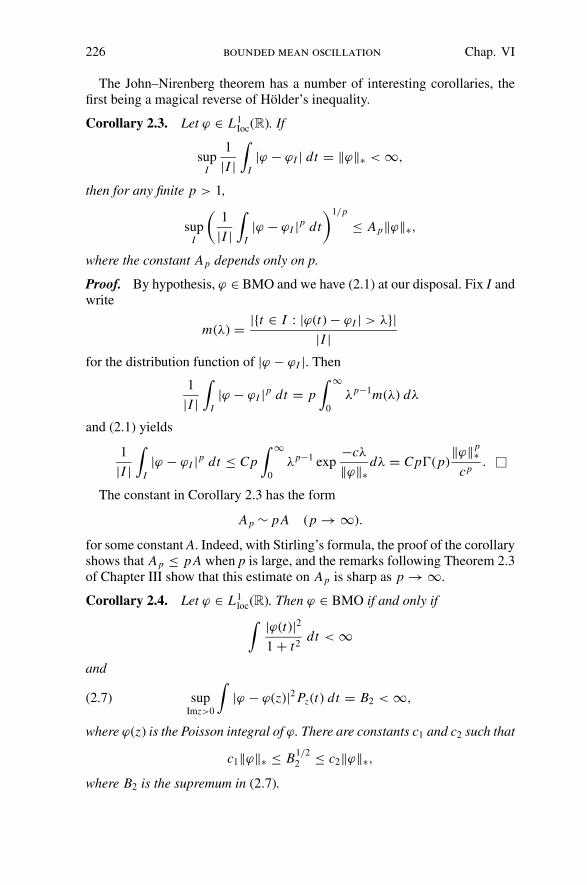
226 bounded mean oscillation Chap. VI
The John–Nirenberg theorem has a number of interesting corollaries, thefirst being a magical reverse of Holder’s inequality.
Corollary 2.3. Let ϕ ∈ L1Ioc(R). If
supI
1
|I |∫
I|ϕ − ϕI | dt = ‖ϕ‖∗ < ∞,
then for any finite p > 1,
supI
(1
|I |∫
I|ϕ − ϕI |p dt
)1/p
≤ Ap‖ϕ‖∗,
where the constant Ap depends only on p.
Proof. By hypothesis, ϕ ∈ BMO and we have (2.1) at our disposal. Fix I andwrite
m(λ) = |{t ∈ I : |ϕ(t) − ϕI | > λ}||I |
for the distribution function of |ϕ − ϕI |. Then
1
|I |∫
I|ϕ − ϕI |p dt = p
∫ ∞
0
λp−1m(λ) dλ
and (2.1) yields
1
|I |∫
I|ϕ − ϕI |p dt ≤ Cp
∫ ∞
0
λp−1 exp−cλ
‖ϕ‖∗dλ = Cp�(p)
‖ϕ‖p∗
cp.
The constant in Corollary 2.3 has the form
Ap ∼ p A (p → ∞).
for some constant A. Indeed, with Stirling’s formula, the proof of the corollaryshows that Ap ≤ p A when p is large, and the remarks following Theorem 2.3of Chapter III show that this estimate on Ap is sharp as p → ∞.
Corollary 2.4. Let ϕ ∈ L1loc(R). Then ϕ ∈ BMO if and only if
∫ |ϕ(t)|21 + t2
dt < ∞
and
supImz>0
∫|ϕ − ϕ(z)|2 Pz(t) dt = B2 < ∞,(2.7)
where ϕ(z) is the Poisson integral of ϕ. There are constants c1 and c2 such that
c1‖ϕ‖∗ ≤ B1/22 ≤ c2‖ϕ‖∗,
where B2 is the supremum in (2.7).

Sect. 2 the john–nirenberg theorem 227
Before giving the proof we note the trivial but useful identity
infα
∫|ϕ − α|2 Pz(t) dt =
∫|ϕ − ϕ(z)|2 Pz(t) dt(2.8)
=∫
|ϕ|2 Pz(t) dt − |ϕ(z)|2,
which holds because in the Hilbert space L2(Pz(t) dt) the orthogonal projectionof ϕ onto the constants is ϕ(z).
Proof. If the Poisson integral of |ϕ|2 converges, and if (2.7) holds, thenHolder’s inequality and Theorem 1.2 show that ϕ ∈ BMO with
‖ϕ‖∗ ≤ c2 B1/22 .
The proof of the converse resembles the proof of Theorem 1.2. Suppose ϕ ∈BMO and fix z = x + iy, y > 0. Let Ik be the interval {|t − x | < 2k y}, k =0, 1, 2, . . . . Then |I0| = 2y and
Pz(t) ≤ c
y, t ∈ I0,
Pz(t) ≤ c
22k y, t ∈ Ik\Ik−1 k = 1, 2, . . . .
Also, by Lemma 1.1,
|ϕ − ϕI0|2 ≤ 2|ϕ − ϕIk |2 + 2|ϕIK − ϕI0
|2 ≤ 2|ϕ − ϕIk |2 + 2c2k2‖ϕ‖2∗.
Hence∫
|ϕ − ϕI0|2 Pz(t) dt ≤ 2c
|I0|∫
I0
|ϕ − ϕI0|2 dt
+∞∑
k=1
2c
2k |Ik |∫
Ik\Ik−1
|ϕ − ϕIk |2 dt
+∞∑
k=1
2c2
2k |Ik |k2‖ϕ‖2∗|Ik |
≤ C22‖ϕ‖2
∗and (2.7) holds.
Corollary 2.5. If ϕ ∈ BMO, then the conjugate function ϕ ∈ BMO, and
c1‖ϕ‖∗ ≤ ‖ϕ‖∗ ≤ c2‖ϕ‖∗
for some constants c1 and c2 not depending on ϕ.
Proof. By Corollary 2.4 it is enough to prove∫
|ϕ − ϕ(z)|2 Pz(t) dt =∫
|ϕ − ϕ(z)|2 Pz(t) dt

228 bounded mean oscillation Chap. VI
for any fixed z ∈ H . This reduces to the identity
1
2π
∫|g|2 dθ = 1
2π
∫|g|2 dθ,
g ∈ L2(T ),∫
g dθ = 0, by means of the conformal mapping from H to Dthat sends z to the origin.
3. Littlewood–Paley Integrals and Carleson Measures
We begin with a classical identity of Littlewood–Paley type. Let g(eiθ ) bean integrable function on T = ∂D, and let g(z), z ∈ D, denote the Poissonintegral of g. The gradient ∇g(z) is the complex vector (∂g/∂x, ∂g/∂y) and itssquared length is
|∇g(z)|2 =∣∣∣∣∂g
∂x
∣∣∣∣
2
+∣∣∣∣∂g
∂y
∣∣∣∣
2
.
In this notation we have
|∇g(z)|2 = 2|g′(z)|2
if g(z) is analytic.Let � be a plane domain with smooth boundary and let u(z) and v(z) be C2
functions on �. Then Green’s theorem states that
∫∫
�
(v �u − u �v) dx dy =∫
∂�
(
v∂u
∂n− u
∂v
∂n
)
ds,
where � is the Laplacian, ∂/∂n is differentiation in the outward normal direc-tion, and ds is arc length on ∂�.
Lemma 3.1. If g(eit ) ∈ L1(T ), and if g(0) = (1/2π )∫
g(θ ) dθ is its meanvalue, then
1
π
∫∫
D
|∇g(z)|2 log1
|z|dx dy = 1
2π
∫|g(eiθ ) − g(0)|2dθ.(3.1)
Proof. We may assume that g(0) = 0. Notice that
2|∇g(z)|2 = �(|g(z)|2).

Sect. 3 littlewood–paley integrals and carleson measures 229
For r < 1, Green’s theorem, with u(z) = |g(z)|2 and v(z) = log(r/|z|), nowyields∫∫
|z|<r
�(|g(z)|2) logr
|z|dx dy =∫
|z|=r|g(z)|2 ds
r
− limε→0
∫
|z|=ε
( |g(z)|2ε
− logr
ε
∂
∂|z| |g(z)|2)
ds.
Since g(0) = 0 and since ∇g(z) is bounded in |z| < 12, the above limit is zero,
and we have∫∫
|z|<r
|∇g(z)|2 logr
|z|dx dy = 12
∫|g(reiθ )|2 dθ.
By monotone convergence the left side of this equality tends to∫∫
D
|∇g(z)|2 log1
|z|dx dy
as r → 1, while the right side has limit 12
∫ |g(eiθ )|2dθ . That proves the lemma.
A slightly different form of (3.1) is sometimes easier to use.
Lemma 3.2. If g(eiθ ) ∈ L1(T ), then
1
π
∫∫
D
|∇g(z)|2(1 − |z|2)dx dy ≤ 1
π
∫|g(eiθ ) − g(0)|2dθ(3.2)
≤ C
π
∫∫
D
|∇g(z)|2(1 − |z|2)dx dy,
where C is some absolute constant.
Proof. The leftmost inequality in (3.2) follows from (3.1) and the simple factthat 1 − |z|2 ≤ 2 log(1/|z|), |z| < 1. To prove the other inequality, supposethat the integral on the right is finite and normalize g(z) so that
1
π
∫∫|∇g(z)|2(1 − |z|2) dx dy = 1.
For |z| > 14, we have the reverse inequality log(1/|z|) ≤ c1(1 − |z|2), which
yields
1
π
∫∫
1/4<|z|<1
|∇g(z)|2 log1
|z|dx dy ≤ c1
π
∫∫
D
|∇g(z)|2(1 − |z|2) dx dy.
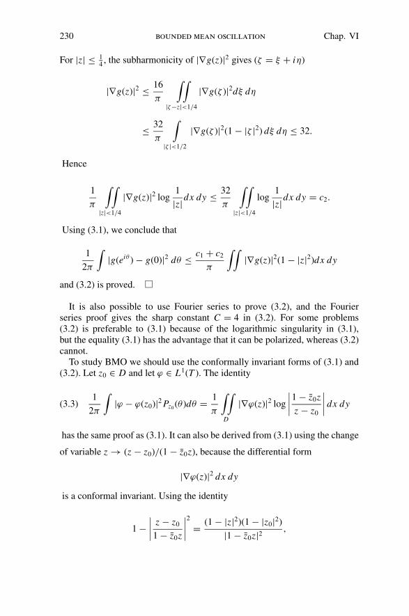
230 bounded mean oscillation Chap. VI
For |z| ≤ 14, the subharmonicity of |∇g(z)|2 gives (ζ = ξ + iη)
|∇g(z)|2 ≤ 16
π
∫∫
|ζ−z|<1/4
|∇g(ζ )|2dξ dη
≤ 32
π
∫
|ζ |<1/2
|∇g(ζ )|2(1 − |ζ |2) dξ dη ≤ 32.
Hence
1
π
∫∫
|z|<1/4
|∇g(z)|2 log1
|z|dx dy ≤ 32
π
∫∫
|z|<1/4
log1
|z|dx dy = c2.
Using (3.1), we conclude that
1
2π
∫|g(eiθ ) − g(0)|2 dθ ≤ c1 + c2
π
∫∫|∇g(z)|2(1 − |z|2)dx dy
and (3.2) is proved.
It is also possible to use Fourier series to prove (3.2), and the Fourierseries proof gives the sharp constant C = 4 in (3.2). For some problems(3.2) is preferable to (3.1) because of the logarithmic singularity in (3.1),but the equality (3.1) has the advantage that it can be polarized, whereas (3.2)cannot.
To study BMO we should use the conformally invariant forms of (3.1) and(3.2). Let z0 ∈ D and let ϕ ∈ L1(T ). The identity
1
2π
∫|ϕ − ϕ(z0)|2 Pz0
(θ )dθ = 1
π
∫∫
D
|∇ϕ(z)|2 log
∣∣∣∣1 − z0z
z − z0
∣∣∣∣ dx dy(3.3)
has the same proof as (3.1). It can also be derived from (3.1) using the change
of variable z → (z − z0)/(1 − z0z), because the differential form
|∇ϕ(z)|2 dx dy
is a conformal invariant. Using the identity
1 −∣∣∣∣
z − z0
1 − z0z
∣∣∣∣
2
= (1 − |z|2)(1 − |z0|2)
|1 − z0z|2 ,
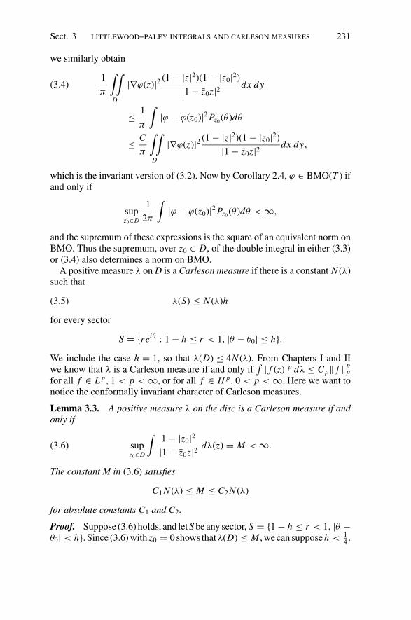
Sect. 3 littlewood–paley integrals and carleson measures 231
we similarly obtain
1
π
∫∫
D
|∇ϕ(z)|2 (1 − |z|2)(1 − |z0|2)
|1 − z0z|2 dx dy(3.4)
≤ 1
π
∫|ϕ − ϕ(z0)|2 Pz0
(θ )dθ
≤ C
π
∫∫
D
|∇ϕ(z)|2 (1 − |z|2)(1 − |z0|2)
|1 − z0z|2 dx dy,
which is the invariant version of (3.2). Now by Corollary 2.4, ϕ ∈ BMO(T ) ifand only if
supz0∈D
1
2π
∫|ϕ − ϕ(z0)|2 Pz0
(θ )dθ < ∞,
and the supremum of these expressions is the square of an equivalent norm onBMO. Thus the supremum, over z0 ∈ D, of the double integral in either (3.3)or (3.4) also determines a norm on BMO.
A positive measure λ on D is a Carleson measure if there is a constant N (λ)such that
λ(S) ≤ N (λ)h(3.5)
for every sector
S = {reiθ : 1 − h ≤ r < 1, |θ − θ0| ≤ h}.We include the case h = 1, so that λ(D) ≤ 4N (λ). From Chapters I and IIwe know that λ is a Carleson measure if and only if
∫ | f (z)|p dλ ≤ C p‖ f ‖pp
for all f ∈ L p, 1 < p < ∞, or for all f ∈ H p, 0 < p < ∞. Here we want tonotice the conformally invariant character of Carleson measures.
Lemma 3.3. A positive measure λ on the disc is a Carleson measure if andonly if
supz0∈D
∫1 − |z0|2|1 − z0z|2 dλ(z) = M < ∞.(3.6)
The constant M in (3.6) satisfies
C1 N (λ) ≤ M ≤ C2 N (λ)
for absolute constants C1 and C2.
Proof. Suppose (3.6) holds, and let S be any sector, S = {1 − h ≤ r < 1, |θ −θ0| < h}. Since (3.6) with z0 = 0 shows thatλ(D) ≤ M , we can suppose h < 1
4.
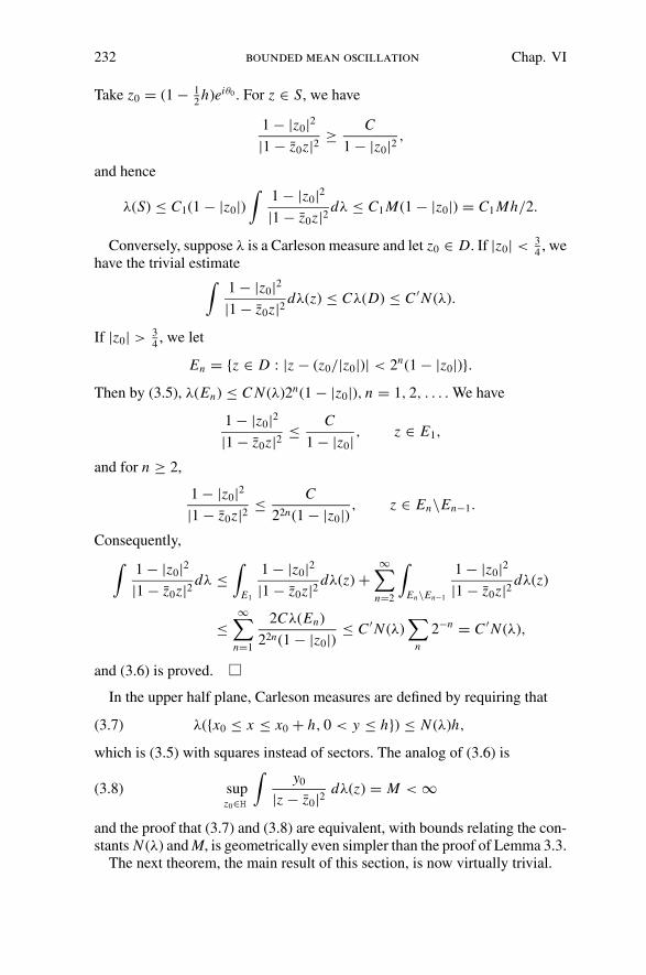
232 bounded mean oscillation Chap. VI
Take z0 = (1 − 12h)eiθ0 . For z ∈ S, we have
1 − |z0|2|1 − z0z|2 ≥ C
1 − |z0|2 ,
and hence
λ(S) ≤ C1(1 − |z0|)∫
1 − |z0|2|1 − z0z|2 dλ ≤ C1 M(1 − |z0|) = C1 Mh/2.
Conversely, suppose λ is a Carleson measure and let z0 ∈ D. If |z0| < 34, we
have the trivial estimate∫
1 − |z0|2|1 − z0z|2 dλ(z) ≤ Cλ(D) ≤ C ′N (λ).
If |z0| > 34, we let
En = {z ∈ D : |z − (z0/|z0|)| < 2n(1 − |z0|)}.Then by (3.5), λ(En) ≤ C N (λ)2n(1 − |z0|), n = 1, 2, . . . . We have
1 − |z0|2|1 − z0z|2 ≤ C
1 − |z0| , z ∈ E1,
and for n ≥ 2,
1 − |z0|2|1 − z0z|2 ≤ C
22n(1 − |z0|) , z ∈ En\En−1.
Consequently,
∫1 − |z0|2|1 − z0z|2 dλ ≤
∫
E1
1 − |z0|2|1 − z0z|2 dλ(z) +
∞∑
n=2
∫
En\En−1
1 − |z0|2|1 − z0z|2 dλ(z)
≤∞∑
n=1
2Cλ(En)
22n(1 − |z0|) ≤ C ′N (λ)∑
n
2−n = C ′N (λ),
and (3.6) is proved.
In the upper half plane, Carleson measures are defined by requiring that
λ({x0 ≤ x ≤ x0 + h, 0 < y ≤ h}) ≤ N (λ)h,(3.7)
which is (3.5) with squares instead of sectors. The analog of (3.6) is
supz0∈H
∫y0
|z − z0|2 dλ(z) = M < ∞(3.8)
and the proof that (3.7) and (3.8) are equivalent, with bounds relating the con-stants N (λ) and M, is geometrically even simpler than the proof of Lemma 3.3.
The next theorem, the main result of this section, is now virtually trivial.

Sect. 3 littlewood–paley integrals and carleson measures 233
Theorem 3.4. Let ϕ ∈ L1(T ), and let
dλϕ = |∇ϕ(z)|2 log1
|z|dx dy,
where ∇ϕ is the gradient of the Poisson integral ϕ(z). Then ϕ ∈ BMO(T ) ifand only if λϕ is a Carleson measure. There are universal constants C1 andC2 such that
C1‖ϕ‖2∗ ≤ N (λϕ) ≤ C2‖ϕ‖2
∗.
Proof. By Corollary 2.4 and by the inequalities (3.4), we know that ϕ ∈BMO(T ) if and only if
supz0∈D
∫∫
D
|∇ϕ(z)|2 (1 − |z|2)(1 − |z0|2)
|1 − z0z|2 dx dy = M1 < ∞(3.9)
and that M1 ≈ ‖ϕ‖2∗. By Lemma 3.3, (3.9) holds if and only if
dμϕ = |∇ϕ(z)|2(1 − |z|2) dx dy
is a Carleson measure, and N (μϕ) ≈ ‖ϕ‖2∗. What remains to be proved are
that μϕ is a Carleson measure if and only if λϕ is a Carleson measure and thatN (λϕ) ≈ N (μϕ). Half of this task is trivial because the inequality 1 − |z|2 <
2 log(1/|z|) shows that μϕ ≤ 2λϕ . For |z| > 14
we have the reverse inequality
log(1/|z|) ≤ C(1 − |z|2),
which shows that
λϕ(S) ≤ Cμϕ(S)
for sectors S = {1 − h ≤ r < 1, |θ − θ0| < h} provided h ≤ 34. This will give
N (λϕ) ≤ C N (μϕ) if we can prove
λϕ({|z| ≤ 1
4}) ≤ Cμϕ({|z| ≤ 1
2}) ≤ C N (μϕ).(3.10)
However, we already touched on (3.10) in the proof of Lemma 3.2. Because|∇ϕ(z)|2 is subharmonic, we have
λϕ({|z| ≤ 1
4}) ≤ C sup
|z|<1/4
|∇ϕ(z)|2 ≤ 32C
π
∫
|ζ |<1/2
|∇ϕ(ζ )|2(1 − |ζ |2) dξ dη
≤ C ′μϕ({|ζ | ≤ 1
2}).
That gives (3.10) and therefore N (λϕ) ≤ C N (μϕ).
The measure λϕ with the logarithm will be used when we polarize the identity(3.1) in the next section. The most important ingredient of Theorem 3.4 is the

234 bounded mean oscillation Chap. VI
John–Nirenberg theorem, which makes it possible to characterize BMO usingquadratic expressions.
4. Fefferman’s Duality Theorem
Let us first digress briefly to find the dual space of H p(dt), 1 ≤ p < ∞.This was done for the disc in Chapter IV, Section 1, and the argument for thehalf plane is formally the same.
Lemma 4.1. If 1 ≤ p < ∞, if q = p/(p − 1), and if g ∈ Lq, then g ∈(H p)⊥, that is,
∫fg dt = 0(4.1)
for all f ∈ H p if and only if g ∈ Hq.
Proof. If g ∈ Hq , then by Holder’s inequality f g ∈ H 1, and (4.1) followsfrom Lemma II.3.7.
On the other hand if (4.1) holds then the Poisson integral of g is analytic onH . Indeed, if z ∈ H and if z0 ∈ H is fixed, then
hz(t) = 1
z − t− 1
z0 − t
is in H p and
Pz − Pz0= 1
2π i(hz − hz).
Hence, by (4.1),
g(z) − g(z0) =∫
g(t)(Pz(t) − Pz0(t)) dt
= − 1
2π i
∫g(t)
(1
z − t− 1
z0 − t
)
dt,
and g(z) is analytic. Theorem I.3.5 now implies that g ∈ H p.
With the Hahn–Banach theorem, the lemma yields
(H p)∗ = Lq/Hq , 1 ≤ p < ∞.(4.2)
In (4.2), the pairing between f ∈ H p and a coset g + Hq ∈ Lq/Hq is givenby
∫f g dt.
Our object in this section is to represent (H p)∗ as a space of functions ratherthan as a quotient space. Two Banach spaces X and Y are said to be isomorphic

Sect. 4 fefferman’s duality theorem 235
if there is a linear mapping T from X onto Y such that
c1‖x‖ ≤ ‖T x‖ ≤ c2‖x‖, x ∈ X.
The isomorphism T from X onto Y is called an isometry if ‖T x‖ = ‖x‖ forall x ∈ X . When two spaces are isomorphic, one thinks of them as being thesame space with two different, but equivalent, norms.
What we are looking for is an isomorphism between (H p)∗ and some spaceof functions. For 1 < p < ∞, the M. Riesz theorem on conjugate functionsgives the isomorphism we want.
Theorem 4.2. For 1 < p < ∞, (H p)∗ is isomorphic to Hq , the space ofcomplex conjugates of functions in Hq. The isomorphism T : Hq → (H p)∗ isdefined by
(T g)( f ) =∫
f g dt, f ∈ H p, g ∈ Hq .(4.3)
Proof. Since 1 < q < ∞, the Hilbert transform H is bounded on Lq . Theoperator
S(g) = g − i Hg
is then also bounded on Lq . The kernel of S is Hq and the range of S is Hq .By the open mapping theorem, the induced mapping
S : Lq/Hq → Hq
is an isomorphism. By (4.2), T = S−1 is an isomorphism of Hq onto (H p)∗ =Lq/Hq . When g ∈ Hq , S(g + Hq ) = g, and hence (4.3) holds.
When p = 1, the above argument does not apply because the Riesz theoremfails for L∞. We shall see that the function space isomorphic to (H 1)∗ =L∞/H∞ is not H∞ but BMO.
It will be convenient to regard H 1 as a Banach space over the real numbersonly. Any complex Banach space X can of course be viewed as a real Banachspace. However, the complex linear functionals on X can be recovered from thereal linear functionals on X in a very simple way. If L is a real linear functionalon X, then
LC(x) = L(x) − i L(i x)
defines a complex linear functional on X, and
L(x) = Re LC(x).
Because ‖LC‖ = sup{Re LC(x) : ‖x‖ = 1}, the functionals L and LC havethe same norm. Hence, the correspondence L → LC is a real linear isometrybetween the space of continuous real linear functionals on X and the realBanach space of complex linear functionals on X.

236 bounded mean oscillation Chap. VI
For example, when 1 < p < ∞, H p is isomorphic, as a real Banach space,to L p
R, the space of real L p functions. Again Riesz’s theorem provides the
isomorphism defined by
L pR
� u → u + i Hu.
Any real linear functional on H p is therefore given by
L(u + i Hu) =∫
uv dt
for a unique v ∈ LqR
. The corresponding complex linear functional is
LC(u + i Hu) =∫
uv dt + i∫
(Hu)v dt.
The identities∫
(Hu)v dt = −∫
u Hv dt,∫
(Hu)(Hv) dt =∫
uv dt,
which follow from Lemma 4.1 or from (1.9) and (1.10) of Chapter III, showthat
LC(u + i Hu) =∫
(u + i Hu)g dt,
where g = (v − i Hv)/2 ∈ Hq . This brings us back to (4.3), and we have, infact, merely rephrased the proof of Theorem 4.2. It is for the case p = 1 thatreal linear functionals simplify the duality problem.
Now suppose p = 1. As a real Banach space, H 1 is isomorphic to the space
H 1R
= {u ∈ L1R
: Hu ∈ L1R}
provided that H 1R
is given the graph norm
‖u‖H 1 = ‖u‖1 + ‖Hu‖1.
This norm is chosen so that
H 1 � f → Re f
is an isomorphism of H 1 onto H 1R
.Recall from Chapter II, Corollary 3.3, that the subset
A = {u ∈ H 1R
: (1 + t2)|u + i Hu| ∈ L∞}is norm dense in H 1
R.
Lemma 4.3. Let L be a continuous real linear functional on H 1R
. Then thereare ϕ1 and ϕ2 in L∞
Rsuch that
‖ϕ1‖∞ ≤ ‖L‖, ‖ϕ2‖∞ ≤ ‖L‖

Sect. 4 fefferman’s duality theorem 237
and such that
L(u) =∫
(uϕ1 − (Hu)ϕ2) dt, u ∈ H 1R.(4.4)
If u ∈ A, then
L(u) =∫
u(ϕ1 + Hϕ2) dt.(4.5)
Moreover, there is a unique real function ϕ ∈ BMO such that
‖ϕ‖∗ ≤ C‖L‖for some universal constant C and such that
L(u) =∫
uϕ dt, u ∈ A.(4.6)
By Theorems 1.2 and 1.5, the integrals in (4.5) and (4.6) are absolutelyconvergent when u ∈ A.
Proof. The space H 1R
is a closed subspace of L1R
⊕ L1R
when this latter spaceis given the norm ‖(u, v)‖ = ‖u‖1 + ‖v‖1. Extend L to a bounded real linearfunctional � on L1
R⊕ L1
Rsuch that ‖�‖ = ‖L‖. Now � has the representation
�(u, v) =∫
(uϕ1 − vϕ2) dt,
where (ϕ1, ϕ2) ∈ L∞R
⊕ L∞R
, and
‖�‖ = max(‖ϕ1‖∞, ‖ϕ2‖∞),
because of the choice of the norm on L1R
⊕ L1R
. Thus, ‖ϕ1‖∞ ≤ ‖L‖, ‖ϕ2‖∞ ≤‖L‖, and (4.4) holds. Since
∫(Hu)ϕ2 dt = −
∫u(Hϕ2) dt
when u ∈ A and ϕ2 ∈ L∞, (4.5) follows from (4.4). Also the function
ϕ = ϕ1 + Hϕ2
is in BMO, and ‖ϕ‖∗ ≤ C‖L‖, by Theorem 1.5. Now (4.6) is obvious, sinceit is just a restatement of (4.5).
It remains to show that ϕ is uniquely determined by L. The pair (ϕ1, ϕ2) ∈L∞
R⊕ L∞
Rcorresponding to L is by no means unique. A pair (ϕ1, ϕ2) induces
the zero functional on H 1R
if and only if∫
u(ϕ1 + Hϕ2) dt = 0, u ∈ A.(4.7)
238 bounded mean oscillation Chap. VI
Since any difference Pz(t) − Pz0(t) of Poisson kernels is in A, this holds if and
only if ϕ1 + Hϕ2 has constant Poisson integral. Thus (4.7) occurs if and onlyif ϕ1 + Hϕ2 is constant. Since constants have zero BMO norm, this means thatL gives rise to a unique BMO function ϕ such that (4.6) holds.
As an aside, we note that ϕ1 + Hϕ2 is constant if and only if ϕ1 + iϕ2 ∈ H∞.Thus the proof of the lemma again shows that (H 1)∗ = L∞/H∞.
Theorem 4.4 (C. Fefferman). The dual space of H 1R
is BMO. More precisely,if ϕ ∈ BMO is real valued and if L is defined by
L(u) =∫
uϕ dt, u ∈ A,(4.8)
then |L(u)| ≤ C1‖ϕ‖∗‖u‖H 1 . Conversely, if L ∈ (H 1R
)∗, then there is a uniquereal ϕ ∈ BMO with ‖ϕ‖∗ ≤ C‖L‖ such that (4.8) holds.
Although the integral in (4.8) makes sense only for u ∈ A, the density of A
in H 1R
and the inequality |L(u)| ≤ C1‖ϕ‖∗‖u‖H 1 enable us now to regard eachϕ ∈ BMO as a continuous linear functional on H 1
R.
Proof. By Lemma 4.3, each L ∈ (H 1R
)∗ yields a unique ϕ ∈ BMO with‖ϕ‖∗ ≤ C‖L‖ such that (4.8) holds. The important thing that remains to beproved is that
∣∣∣∣
∫uϕ dt
∣∣∣∣ ≤ C1‖ϕ‖∗‖u‖H 1, u ∈ A,(4.9)
whenever ϕ ∈ BMO. The proof of the corresponding inequality on the unitcircle is a little less technical, and instead of (4.9) we prove
∣∣∣∣
∫uϕ
dθ
2π
∣∣∣∣ ≤ C1‖ϕ‖∗‖u + i u‖1(4.10)
for u ∈ L2R
(T ) and for ϕ ∈ BMO(T ) with∫
ϕ dθ = 0. Now, if u ∈ A and ifϕ ∈ BMO(R), then, with eiθ = (t − i)/(t + i), dθ = 2 dt/(1 + t2),
∫uϕ dt = 1
2
∫U (θ ) �(θ ) dt
where U (θ ) = (1 + t2) u(t) ∈ L2R
(T) and �(θ ) = ϕ(t) ∈ BMO (T). Then
(U + iU )(eiθ ) = (u + i u)(t)
( −4eiθ
(eiθ − i)2
)
∈ H2
has mean value zero. Hence ‖U + iU‖1 = 2‖u + i u‖1 and by Corollary 1.3,inequality (4.10) implies inequality (4.9).
Now, let u ∈ L2R
(T ) and let ϕ ∈ BMO(T ). Notice that, by Corollary 2.4and Corollary 1.3, the integral (4.10) converges absolutely. Let f = u + i Hu.

Sect. 4 fefferman’s duality theorem 239
Then f ∈ H 1, and
∫uϕ
dθ
2π= Re
∫f ϕ
dθ
2π.
The advantage of working with f instead of with u is that we may suppose thatf = g2, g ∈ H 2. Indeed, write f = B F , where B is a Blaschke product, F ∈H 1 has no zeros in D, and ‖F‖1 = ‖ f ‖1. Write f1 = (B − 1)F and f2 = (B +1)F . Then ‖ f1‖1 ≤ 2‖ f ‖1, ‖ f2‖1 ≤ 2‖ f ‖1, and f = ( f1 + f2)/2. Moreoverf1 and f2 have no zeros in D, so that f1 and f2 are both of the form g2, g ∈ H 2.In estimating
∫f ϕ dθ , we may replace f by f1 or by f2. Thus, we assume
f = g2, g ∈ H 2.We can also assume ϕ(0) = 0. Polarization of the Littlewood–Paley identity,
Lemma 3.1, then yields
∫f ϕ
dθ
2π=
∫( f − f (0))ϕ
dθ
2π= 1
π
∫∫
D
(∇ f ) · (∇ϕ) log1
|z|dx dy.
Since f (z) is analytic, we have
∇ f · ∇ϕ = fxϕx + fyϕy = f ′(z)(ϕx + iϕy) = 2g(z)g′(z)(ϕx + iϕy),
and so
|∇ f · ∇ϕ| ≤ 2|g(z)||g′(z)||∇ϕ(z)|.The Cauchy–Schwarz inequality now gives us
∣∣∣∣
∫f ϕ
dθ
2π
∣∣∣∣ ≤
⎛
⎝ 2
π
∫∫
D
|g′(z)|2 log1
|z|dx dy
⎞
⎠
1/2
×⎛
⎝ 2
π
∫∫
D
|g(z)|2|∇ϕ(z)|2 log1
|z|dx dy
⎞
⎠
1/2
.
By Lemma 3.1, the first factor is
(1
2π
∫|g(eiθ ) − g(0)|2dθ
)1/2
= ‖ f ‖1/21 .
By Theorem 3.4 and by the disc version of the theorem on Carleson measures,
the second factor is bounded by C‖ϕ‖∗‖ f ‖1/21 . These give us (4.10), and the
theorem is proved.
To prove (4.9) without moving to the circle, see Exercise 6.
240 bounded mean oscillation Chap. VI
The complex linear functional on H 1 determined by ϕ ∈ BMO by use of(4.8) is
LC(u + i Hu) =∫
(u + i Hu)ϕ dt
because Re(−i(u + i Hu)) = Hu. We now have a real linear isomorphismbetween the complex Banach space (H 1)∗ and the real space of real BMOfunctions. In order to regard BMO as a complex space isomorphic to (H 1)∗,observe that
i LC(u + i Hu) = LC(−Hu + iu) =∫
(−Hu + iu)ϕ dt.
By (4.5) and (4.6), the last integral equals∫
(u + i Hu)Hϕ dt,
at least when u ∈ A. If we were to define multiplication by i on the space of realBMO functions iϕ = Hϕ, then real BMO would become a complex Banachspace isomorphic to (H 1)∗, with the complex linear isomorphism from L∞/H∞to real BMO given by L∞/H∞ � f → Re f + H (Im f ). This unusual notionof complex scalar multiplication, which is brought about by identifying H 1
R
with H 1, is one reason that real linear functionals on H 1 are easier to discuss.
Corollary 4.5. If ϕ ∈ L1loc, then ϕ ∈ BMO if and only if
ϕ = ϕ1 + Hϕ2 + α,(4.11)
where α is a constant and where ϕ1 and ϕ2 are L∞ functions. When ϕ ∈BMO, ϕ1 and ϕ2 can be chosen so that
‖ϕ1‖∞ ≤ C‖ϕ‖∗, ‖ϕ2‖∞ ≤ C‖ϕ‖∗(4.12)
for some constant C.
Proof. This corollary is equivalent to the theorem. Theorem 1.5 tells us thatevery function of the form (4.11) is in BMO that
‖ϕ‖∗ ≤ C(‖ϕ1‖∞ + ‖ϕ2‖∞).(4.13)
If ϕ ∈ BMO, then by (4.9), the functional L(u) = ∫uϕ dt, u ∈ A, is bounded
against ‖u‖H 1 . By Lemma 4.3, there are ϕ1, ϕ2 ∈ L∞ such that
L(u) =∫
u(ϕ1 + Hϕ2) dt.
As we observed after the proof of Lemma 4.3, this means that ϕ − (ϕ1 + Hϕ2)has constant Poisson integral. Consequently (4.11) and (4.12) hold.
A constructive proof of (4.11), and hence of the duality theorem itself, willbe given in Chapter VIII.

Sect. 4 fefferman’s duality theorem 241
Because of (4.12) and (4.13), the expression
inf{‖ϕ1‖∞ + ‖ϕ2‖∞ : ϕ = ϕ1 + Hϕ2 + α}defines a norm on BMO equivalent to ‖ϕ‖∗.
Corollary 4.6. Let f ∈ L∞. Then the distance
dist( f, H∞) = infg∈H∞
‖ f − g‖∞
satisfies
C1‖ f − i H f ‖∗ ≤ dist( f, H∞) ≤ C2‖ f − i H f ‖∗(4.14)
for some absolute constants C1 and C2.
Proof. By (4.2) and the Hahn–Banach theorem, we have
dist( f, H∞) = sup
{∣∣∣∣
∫f F dt
∣∣∣∣ : F ∈ H 1, ‖F‖1 ≤ 1
}
.
By density, we may suppose F = u + i Hu, where u ∈ A. Then,∫
f F dt =∫
f u dt + i∫
f Hu dt =∫
( f − i H f )u dt.
Taking the real and imaginary parts of the last integral, we see that (4.14)follows directly from the theorem.
Corollary 4.7. Let f ∈ L∞ be real valued. Then the distances
dist( f, Re H∞) = infg∈H∞
‖ f − Re g‖∞
and
dist∗(H f, L∞) = infϕ∈L∞
‖H f − ϕ‖∗
satisfy
C1 dist( f, Re H∞) ≤ dist∗(H f, L∞) ≤ C2 dist( f, Re H∞)
for some absolute constants C1 and C2.
Proof. If g ∈ H∞, then Im g ∈ L∞ and H f − Im g = H ( f − Re g), so thatby Theorem 1.5,
‖H f − Im g‖∗ ≤ C2‖ f − Re g‖∗.
Thus, we have
dist∗(H f, L∞) ≤ C2 dist( f, Re H∞).

242 bounded mean oscillation Chap. VI
The other inequality asserted in the corollary lies deeper and uses the dualitytheorem. If ϕ ∈ L∞, then by Corollary 4.5,
H f − ϕ = ϕ1 + Hϕ2 + α,
where
‖ϕ1‖∞ + ‖ϕ2‖∞ ≤ C‖H f − ϕ‖∗.
Then
u = ϕ + ϕ1 + α ∈ L∞
and
Hu = Hϕ + Hϕ1 = ϕ2 − f,
so that g = −Hu + iu is in H∞. Also
‖ f − Re g‖∞ = ‖ f + Hu‖∞ = ‖ϕ2‖∞ ≤ C‖H f − ϕ‖∗.
Thus, we have
C1 dist( f, Re H∞) ≤ dist∗(H f, L∞),
and Corollary 4.7 is proved.
A method of estimating dist∗(ϕ, L∞) in terms of the exponential in-tegrability of |ϕ − ϕI | will be given in Section 6.
5. Vanishing Mean Oscillation
Let ϕ ∈ L1loc(R). For δ > 0, write
Mδ(ϕ) = sup|I |<δ
1
|I |∫
I|ϕ − ϕI | dt,(5.1)
where I denotes an interval. Then ϕ ∈ BMO if and only if Mδ(ϕ) is boundedand ‖ϕ‖∗ = limδ→∞ Mδ(ϕ). We say that ϕ has vanishing mean oscillation, ϕ ∈VMO, if
(i) ϕ ∈ BMO and(ii) M0(ϕ) = limδ→0 Mδ(ϕ) = 0.
It is easy to see that VMO is a closed subspace of BMO. The relation betweenBMO and the subspace VMO is quite similar to the relation between L∞ andits subspace of bounded uniformly continuous functions. Write UC for thespace of uniformly continuous functions on R and write BUC for L∞∩ UC.
Theorem 5.1. For a function ϕ ∈ BMO, the following conditions are equiv-alent:
Sect. 5 vanishing mean oscillation 243
(a) ϕ ∈ VMO.(b) If ϕx (t) = ϕ(t − x) is the translation of ϕ by x units, then
limx→0
‖ϕx − ϕ‖∗ = 0.
(c) If ϕ(t, y) = Py ∗ ϕ is the Poisson integral of ϕ, then
limy→0
‖ϕ(t) − ϕ(t, y)‖∗ = 0.
(d) ϕ is in the BMO closure of UC ∩ BMO;
infg∈UC ∩ BMO
‖ϕ − g‖∗ = 0.
Proof. We verify the circle of implications (a) ⇒ (b) ⇒ (c) ⇒ (d) ⇒ (a).Assume (a) holds. Let δ > 0 and partition R into intervals
I j = ( jδ/2, ( j + 1)δ/2), −∞ < j < ∞,
of length δ/2. By (5.1) we have
|ϕI j − ϕI j+1| ≤ 2Mδ(ϕ).(5.2)
Define
h(t) =∞∑
j=−∞ϕI j χI j (t).
We first show that
‖ϕ − h‖∗ ≤ 5Mδ(ϕ).(5.3)
If |I | ≤ δ, then by (5.2) we have
1
|I |∫
I|h − hI | dt ≤ 4Mδ(ϕ),
so that
1
|I |∫
I|(ϕ − h) − (ϕ − h)I | dt ≤ 5Mδ(ϕ).
If |I | > δ and if J is the union of those I j such that I j ∩ I �= ∅, then |J | ≤ 2|I |.Writing J = I1 ∪ I2 ∪ · · · ∪ IN , we have
1
|I |∫
I|(ϕ − h) − (ϕ − h)I | dt ≤ 2
|I |∫
I|ϕ − h| dt ≤ 4
|J |∫
J|ϕ − h| dt
≤ 4
N
N∑
j=1
1
|I j |∫
I j
|ϕ − ϕI j | dt ≤ 4Mδ(ϕ),
244 bounded mean oscillation Chap. VI
and (5.3) is proved. Now if |x | < δ, then by (5.2), ‖h − hx‖∞ ≤ 2Mδ(ϕ), sothat ‖h − hx‖∗ ≤ 2Mδ(ϕ). Consequently, if |x | < δ, then
‖ϕ − ϕx‖∗ ≤ ‖ϕ − h‖∗ + ‖h − hx‖∗ + ‖ϕx − hx‖∗= 2‖ϕ − h‖∗ + ‖h − hx‖∗ ≤ 12Mδ(ϕ).
This proves that (a) implies (b).Now assume (b) holds. Then
ϕ(t, y) =∫
ϕ(t − x)Py(x) dx
is an average of the translates ϕx of ϕ. By (b), ‖ϕ − ϕx‖∗ is small if |x | is small,say, if |x | < δ, while for any x, ‖ϕ − ϕx‖∗ ≤ 2‖ϕ‖∗. But when y is small, mostof the weight of Py(x) is given to |x | < δ, and this means that ‖ϕ(t) − ϕ(t, y)‖∗is small. To be precise, by Fubini’s theorem we have
‖ϕ(t) − ϕ(t, y)‖∗ ≤∫
|x |<δ
‖ϕ − ϕx‖∗ Py(x)dx + 2‖ϕ‖∗∫
|x |>δ
Py(x) dx,
so that
limy→0
‖ϕ(t) − ϕ(t, y)‖∗ ≤ sup|x |<δ
‖ϕ − ϕx‖∗.
Hence (b) implies (c).To prove that (c) implies (d), we use the estimate
y|∇ϕ(x, y)| ≤ c‖ϕ‖∗,(5.4)
which is easy to prove. When ϕ ∈ L∞, (5.4) can be derived from Harnack’sinequality and a change of scale, and the extension to ϕ ∈ BMO then followsfrom Corollary 4.5. However, there is also an elementary proof of (5.4) usingTheorem 1.2 instead of the duality theorem. The simple inequality
y|∇ Py(x − t)| ≤ cPy(x − t),
in which the derivatives are taken with respect to x and y, combines withTheorem 1.2 to give
y|∇ϕ(x, y)| ≤ y∫
|ϕ(t) − ϕ(x, y)||∇ Py(x − t)| dt
≤ c∫
|ϕ(t) − ϕ(x, y)|Py(x − t) dt ≤ c‖ϕ‖∗.
Now (5.4) shows that ϕ(x, y) is a uniformly continuous function of x. Becauseϕ(x, y) ∈ BMO, we see that (d) follows from (c).
It is trivial that (d) implies (a), because UC ∩ BMO ⊂ VMO and becauseVMO is closed in BMO.

Sect. 5 vanishing mean oscillation 245
Theorem 5.2. If ϕ is a locally integrable function on R, then ϕ ∈ VMO ifand only if
ϕ = ϕ1 + Hϕ2 + α,(5.5)
where ϕ1, ϕ2, ∈ BUC and where α is a constant. When ϕ ∈ VMO, ϕ1 and ϕ2
can be chosen in BUC so that (5.5) holds and so that
‖ϕ1‖∞ + ‖ϕ2‖∞ ≤ C‖ϕ‖∗,(5.6)
where C is a constant not depending on ϕ.
Proof. Suppose that ϕ has the form (5.5), with ϕ1, ϕ2 ∈ BUC. Then ϕ ∈BMO, and for |x | small, ‖ϕ j − (ϕ j )x‖∞ < ε, j = 1, 2. Therefore
‖ϕ1 − (ϕ1)x‖∗ < ε and ‖(Hϕ2) − (Hϕ2)x‖∗ < ε
when |x | is small, so that by Theorem 5.1(b) ϕ ∈ VMO.Conversely, if ϕ ∈ VMO, then by Corollary 4.5,
ϕ = u1 + Hu2 + α,
where ‖u1‖∞ ≤ C‖ϕ‖∗, ‖u2‖∞ ≤ C‖ϕ‖∗, and α is constant. By Theorem
5.1, there is y0 > 0 such that ‖ϕ(x) − ϕ(x, y0)‖∗ < ‖ϕ‖∗/2. Let ϕ(1)1 (x) =
u1(x, y0), ϕ(1)2 (x) = u2(x, y0). Then ϕ
(1)j ∈ BUC,
‖ϕ(1)j ‖∞ ≤ ‖u j‖∞ ≤ C‖ϕ‖∗, j = 1, 2,
and ϕ(x, y0) = ϕ(1)1 (x) + Hϕ
(1)2 (x) + α, so that
‖ϕ − (ϕ(1)1 + Hϕ
(1)2 + α)‖∗ = ‖ϕ(x) − ϕ(x, y0)‖∗ ≤ ‖ϕ‖∗/2.
Hence
R1 = ϕ − (ϕ(1)1 + Hϕ
(1)2 + α) = (u1 − ϕ
(1)1 ) + H (u2 − ϕ
(1)2 )
is in VMO and ‖R1‖∗ ≤ ‖ϕ‖∗/2. Repeating the above argument with R1 anditerating, we obtain
ϕ =∞∑
k=1
ϕ(k)1 + H
( ∞∑
k=1
ϕ(k)2
)
+ α
with ϕ(k)1 ∈ BUC, ϕ
(k)2 ∈ BUC, and∑
k
‖ϕ(k)1 ‖∞ +
∑
k
‖ϕ(k)2 ‖∞ ≤ 4C‖ϕ‖∗.
That proves Theorem 5.2.
For the circle the proofs of Theorems 5.1 and 5.2 show that VMO is theclosure of C = C(T ) in BMO and that VMO = C + C .

246 bounded mean oscillation Chap. VI
In Chapter IX we shall see that VMO is an important tool in the study of thealgebra H∞ + C .
6. Weighted Norm Inequalities for Maximal Functionsand Conjugate Functions
Let 1 < p < ∞ and let μ be a positive Borel measure on R, finite on compactsets. We consider two problems.
Problem 1. When is the Hardy–Littlewood maximal operator bounded onL p(μ)? That is, when is there a constant Bp such that
∫|M f |pdμ ≤ Bp
∫| f |pdμ
for all measurable functions f (x), where
M f (x) = supx∈I
1
|I |∫
I| f | dt?
Problem 2. When is the Hilbert transform a bounded operator on L p(μ)?That is, when is there a constant C p such that
∫|H f |pdμ ≤ C p
∫| f |pdμ
for all functions f ∈ L2(dx), where
H f (x) = limε→0
1
π
∫
|x−t |>ε
f (t)
x − tdt?
When dμ = dx we know that both operators are bounded for all p, 1 < p <
∞. In the case p = 2, the Helson–Szego theorem, Theorem IV.3.4, providesa necessary and sufficient condition that the Hilbert transform be bounded onL2(μ). The condition is that μ must be absolutely continuous, dμ = w(x) dx ,and the density w(x) must have the form
log w = u + Hv
with u ∈ L∞ and ‖v‖∞ < π/2.The proof of this theorem was given in Chapter IV for the unit circle, but
by now the reader should have no difficulty transferring the theorem to theline. For p �= 2 the Helson–Szego method has not produced very satisfyinganswers to Problem 2.
On the other hand, the real-variables approach to these problems taken byMuckenhoupt and others has been quite successful. Pleasantly, both problemshave the same answer: The measure must be absolutely continuous
dμ = w(x) dx, w ∈ L1loc,

Sect. 6 weighted norm inequalities 247
and the weight w(x) must satisfy the (Ap) condition,
supI
(1
|I |∫
Iw dx
) (1
|I |∫
I
(1
w
)1/(p−1)
dx
)p−1
< ∞.(6.1)
Theorem 6.1. Let μ be a positive measure finite on compact sets, and let1 < p < ∞. Then
∫|M f |pdμ ≤ Bp
∫| f |pdμ
with Bp independent of f if and only if μ is absolutely continuous, dμ =w(x)dx, and the density w(x) satisfies (6.1).
Theorem 6.2. Let μ be a positive measure finite on compact sets and let1 < p < ∞. Then
∫|H f |pdμ ≤ C p
∫| f |pdμ
with C p independent of f if and only if dμ = w(x) dx and the density w(x)satisfies (6.1).
Before going further, let us try to understand how the (Ap) condition (6.1)comes about.
Lemma 6.3. If 1 < p < ∞ and if μ is a positive measure on R such that∫
|M f |pdμ ≤ C∫
| f |pdμ
for all f, then μ is absolutely continuous, dμ = w(x) dx, and w(x) satisfiesthe (Ap) condition (6.1).
Proof. Let E be a compact set with |E | = 0, let ε > 0, and let V be an openneighborhood of E with μ(V \E) < ε. Then f = χV \E has
∫ | f |pdμ < ε. Onthe other hand, M f (x) = 1 when x ∈ E because |E | = 0. Hence by hypothesis,
μ(E) ≤∫
|M f |pdμ ≤ C‖ f ‖pp ≤ Cε,
so that μ(E) = 0 and μ is absolutely continuous.Write dμ = w(x)dx , when w(x) ∈ L1
loc and w(x) ≥ 0. Fix an interval I andlet f (x) = w(x)αχI (x), for some real α. Then
∫| f |pdμ =
∫
Iw(x)1+pα dx,
and if x ∈ I ,
M f (x) ≥ 1
|I |∫
If dt ≥ 1
|I |∫
Iwα dt.

248 bounded mean oscillation Chap. VI
Approximating f (x) from below by bounded functions, we obtain(∫
Iw dx
) (∫
Iwα dx
)p
≤ |I |p∫
I|M f |pdμ ≤ C |I |p
∫
Iw1+pα dx,
and taking α = −1/(p − 1) = 1 + pα, we conclude that
(∫
Iw dx
) (∫
I
(1
w
)1/(p−1)
dx
)p−1
≤ C |I |p,
which is the (Ap) condition.
Lemma 6.4. If 1 < p < ∞ and if μ is a positive measure on R, finite oncompact sets, such that for all f
∫|H f |pdμ ≤ C
∫| f |pdμ,
then dμ = w(x)dx, where w(x) satisfies the (Ap) condition (6.1).
Proof. Testing the hypothesis of the lemma with f = χ[0,1], we see that∫
dμ(x)
(1 + |x |)p< ∞.(6.2)
Let g ∈ Lq (μ), q = p/(p − 1), be real. Then by the hypothesis and by duality,there is h ∈ Lq (μ) such that
∫(H f )g dμ =
∫f h dμ, f ∈ L p(μ).
If f ∈ H 2 ∩ L p(μ), then H f = −i f and the above identity becomes∫
f (g − ih) dμ = 0.(6.3)
By (6.2) and Holder’s inequality,
dν(x) = (g − ih)(x) dμ(x)
x + i
is a finite measure, and by (6.3)∫
(x − z)−1dν(x) = 0 on Im z < 0. The Fand M. Riesz theorem now implies that ν is absolutely continuous. Henceg(x)dμ(x) = Re((x + i)dν(x)) is absolutely continuous. Since g ∈ Lq (μ) isarbitrary, we conclude that μ is absolutely continuous.
Write dμ = w(x)dx . Let I be an interval, and split I into two equal pieces,I = I1 ∪ I2, |I1| = |I2| = 1
2|I |. Let f ≥ 0, f supported in I1. Then for x ∈ I2
we have
|H f (x)| = 1
π
∫
I1
f (t)
|x − t | dt ≥ 1
2π
∫
I1
f (t)
|I1| dt = 1
2πf I1
.(6.4)

Sect. 6 weighted norm inequalities 249
Taking f = χI1, we get
∫
I2
w dx ≤ C∫
I1
w dx .
By symmetry we also have∫
I1
w dx ≤ C∫
I2
w dx .
Taking f = w(x)αχI1in (6.4), we then get
(∫
I2
w dx
) (1
|I1|∫
I1
wα dx
)p
≤ C∫
I1
w1+αp dx .
Setting α = −1/(p − 1) now gives
(∫
I1
w dx
) (1
|I1|∫
I1
(1
w
)1/(p−1)
dx
)p
≤ C∫
I1
(1
w
)1/(p−1)
dx,
which is the (Ap) condition.
Thus (Ap) is a necessary condition in both Theorem 6.1 and Theorem 6.2.Now suppose w satisfies (Ap) and write
ϕ = log w, ψ = log
((1
w
)1/(p−1))
= −ϕ
p − 1.
Then ϕ and ψ are locally integrable, because w and 1/w are. For any intervalI, we have
eϕI (eψI )p−1 = 1
trivially, so that (Ap) can be rewritten
supI
(1
|I |∫
Ieϕ−ϕI dx
) (1
|I |∫
Ieψ−ψI dx
)p−1
< ∞.(6.5)
By Jensen’s inequality,
1
|I |∫
Ieϕ−ϕI dx ≥ 1 and
1
|I |∫
Ieψ−ψI dx ≥ 1.
Consequently (Ap) holds if and only if each factor in (6.5) is bounded sepa-rately, and we have the following lemma.
Lemma 6.5. Let w ≥ 0, and let ϕ = log w. Then w has (Ap), 1 < p < ∞,if and only if
supI
1
|I |∫
Ieϕ−ϕI dx < ∞

250 bounded mean oscillation Chap. VI
and
supI
1
|I |∫
Ie−(ϕ−ϕI )/(p−1)dx < ∞.
Thus if w has (Ap), then ϕ = log w ∈ BMO. Conversely if log w ∈ BMO,then by the John–Nirenberg theorem, wδ has (Ap) for some δ > 0.
Before turning to the more difficult proof that (Ap) is sufficient, we men-tion two corollaries. The case p = 2 of Theorem 6.2 can be merged with theHelson–Szego theorem to give concrete expressions for the BMO distance ofϕ ∈ BMO to L∞ and for the distance from f ∈ L∞
Rto Re H∞. The reason is
that the Helson–Szego condition is, by Theorem 6.2, equivalent to
(A2) : supI
(1
|I |∫
Iw dx
) (1
|I |∫
I
1
wdx
)
< ∞.
If ϕ ∈ BMO, then ϕ = f + Hg + α with f ∈ L∞, g ∈ L∞, and α constant,and
‖ϕ‖′ = inf{‖ f ‖∞ + ‖ f ‖∞ : ϕ = f + Hg + α}defines a norm on BMO equivalent to ‖ϕ‖∗. With respect to ‖ ‖′ the distancefrom ϕ to L∞ is
dist(ϕ, L∞) = inff ∈L∞
‖ϕ − f ‖′ = inf{‖g‖∞ : ϕ − Hg ∈ L∞}.
By the John–Nirenberg theorem there are ε > 0 and λ(ε) > 0 such that
supI
|{x ∈ I : |ϕ − ϕI | > λ}||I | ≤ e−λ/ε, λ > λ(ε).(6.6)
Write
ε(ϕ) = inf{ε > 0 : (6.6) holds}.Clearly ε(ϕ) = 0 if ϕ ∈ L∞. The John–Nirenberg theorem shows that
ε(ϕ) ≤ C‖ϕ‖∗ ≤ C ′‖ϕ‖′.
Corollary 6.6. If ϕ ∈ BMO is real valued, then
dist(ϕ, L∞) = (π/2)ε(ϕ).
Proof. Condition (6.6) implies that
M = supI
1
|I |∫
Iexp |Aϕ − AϕI |dx < ∞(6.7)
whenever A < 1/ε(ϕ), and Chebychev’s inequality shows that A ≤ 1/ε(ϕ)whenever (6.7) holds for A. Thus
1/ε(ϕ) = sup{A : ϕ has (6.7)}.

Sect. 6 weighted norm inequalities 251
By (6.7) we have
1 ≤ 1
|I |∫
Ie±A(ϕ−ϕI )dx ≤ M(6.8)
for any interval I. Conversely, since e|x | ≤ ex + e−x (6.8) implies (6.7). Thus(6.8) is equivalent to (6.7). Hence by Lemma 6.5, (6.7) holds for A > 0 if andonly if the weight w = eAϕ satisfies the (A2) condition. We conclude that
1/ε(ϕ) = sup{A : eAϕ has (A2)}.Because the (A2) condition is equivalent to the Helson–Szego condition, we
now have
1/ε(ϕ) = sup{A : Aϕ = f + Hg, f ∈ L∞, ‖g‖∞ < π/2},which is the same thing as
(π/2)ε(ϕ) = inf{‖g‖∞ : ϕ = f + Hg, f ∈ L∞}.Corollary 6.7. If f ∈ L∞ is real valued, then
dist( f, Re H∞) = infF∈H∞
‖ f − Re F‖∞
satisfies
dist( f, Re H∞) = (π/2)ε(H f ).
Proof. This is immediate from Corollary 6.6 and the proof ofCorollary 4.7.
The distances in Corollaries 6.6 and 6.7 can also be related to the growth ofthe local L p oscillations of ϕ(x) by means of the identity
ε(ϕ)
e= lim
p→∞1
p
(
supI
1
|I |∫
I|ϕ − ϕI |pdx
)1/p
.
Establishing this identity is a recreation left for the reader. See Exercise 17.To show that (Ap) implies the boundedness of M and H on L p(w dx), we
need four consequences of
(Ap) : supI
(1
|I |∫
Iw dx
) (1
|I |∫
I
(1
w
)1/(p−1)
dx
)p−1
< ∞.
The first two consequences are quite trivial.
Lemma 6.8. If 1 < p < ∞ and if w(x)′ satisfies (Ap), then
(a) w(x) satisfies (Ar ) for all r > p, and(b) the weight (1/w)1/(p−1) satisfies (Aq ), where q = p/(p − 1).

252 bounded mean oscillation Chap. VI
Proof. For (a) note that 1/(r − 1) < 1/(p − 1), so that by Holder’s inequality
1
|I |∫
I
(1
w
)1/(r−1)
dx ≤(
1
|I |∫
I
(1
w
)1/(p−1)
dx
)(p−1)/(r−1)
.
For (b) note that 1/(p − 1) = q − 1, so that if v = (1/w)1/(p − 1), then(1/v)1/(q−1) = w.
The other two consequences of (Ap) lie deeper, but they can be derived froma delightful inequality due to Gehring.
Theorem 6.9. Let p > 1. If v(x) ≥ 0, and if
(1
|I |∫
Iv pdx
)1/p
≤ K1
|I |∫
Iv dx(6.9)
for all subintervals of some interval I0, then
(1
|I0|∫
I0
vr dx
)1/r
≤ C(p, K , r )
(1
|I0|∫
I0
v dx
)
(6.10)
for p ≤ r < p + η, where η = η(p, K ) > 0.
The inequality reverse to (6.9), with constant 1, follows trivially fromHolder’s inequality. Therefore the constant K in (6.9) must obviously sat-isfy K ≤ 1. Theorem 6.9 is a close relative of the John–Nirenberg theoremand, as with that theorem, it is crucial that (6.9) hold for many subintervals ofI0.
Proof. We can suppose that I0 = [0, 1] and that∫
I0v p dx = 1. For λ > 0
write
Eλ = {x ∈ I0 : v(x) > λ}.What we are going to prove is the estimate
∫
Eλ
v p dx ≤ Aλp−1
∫
Eλ
v dx, λ ≤ 1,(6.11)
with some constant A = A(p, K ). But first let us observe how (6.11) easilygives (6.10). For r > p we have
∫
E1
vr dx =∫
E1
v pvr−pdx =∫
E1
v p
(
1 + (r − p)
∫ v
1
λr−p−1dλ
)
dx
=∫
E1
v pdx + (r − p)
∫ ∞
1
λr−p−1
∫
Eλ
v pdx dλ.

Sect. 6 weighted norm inequalities 253
By (6.11) the last term in the above expression does not exceed
A(r − p)
∫ ∞
1
λr−2
∫
Eλ
v dx dλ ≤ A(r − p)
∫
E1
v
∫ v
0
λr−2 dλ
= A(r − p)
(r − 1)
∫
E1
vr dx .
Hence(
1 − A(r − p)
(r − 1)
) ∫
E1
vr dx ≤∫
E1
v p dx .
Taking A > 1, we have A(r − p)/(r − 1) < 1 if r < p + (p − 1)/(A − 1) =p + η, η + 0. For such values of r we then have
∫
I0
vr dx ≤∫
{v<1}v p dx + Cr
∫
E1
v p dx .
Because of (6.9) and the normalizations I0| = 1,∫
I0vp dx = 1, this proves
(6.10) and the theorem.To prove (6.11) we set β = 2Kλ > λ ≥ 1. Since trivially
∫
Eλ\Eβ
v p dx ≤ β p−1
∫
Eλ\Eβ
v dx ≤ (2K )p−1λp−1
∫
Eλ
v dx,(6.12)
proving (6.11) really amounts to making an estimate of∫
Eβv p dx . By the
Calderon–Zygmund Lemma 2.2, there are pairwise disjoint subintervals {I j }of I0 such that
β p ≤ 1
|I j |∫
I j
v p dx < 2β p(6.13)
and such that v ≤ β almost everywhere on I0\⋃
I j . So except for a set ofmeasure zero, we have Eβ ⊂ ⋃
I j . By (6.13) we have
∫
Eβ
v p dx ≤∑
j
∫
I j
v p dx ≤ 2β p∑
j
|I j |.(6.14)
By (6.9) and the other inequality in (6.13), we also have
β ≤(
1
|I | j
∫
I j
v p dx
)1/p
≤ K
|I | j
∫
I j
v dx .
This means that
|I j | ≤ K
β
∫
I j
v dx ≤ K
β
∫
I j ∩Eλ
v dx + Kλ
β|I j |,

254 bounded mean oscillation Chap. VI
so that by our choice of β,
|I j | ≤ 1
λ
∫
I j ∩Eλ
v dx .
Substituting this inequality into (6.14) gives∫
Eβ
v p dx ≤ 2β p
λ
∫
Eλ
v dx ≤ 2p+1 K pλp−1
∫
Eλ
v dx,
and with (6.12) this yields the desired inequality (6.11).
Corollary 6.10. If 1 < p < ∞ and if the weight w(x) satisfies the (Ap)condition, then
(a) there are δ > 0 and C > 0 such that, for any interval I,(
1
|I |∫
Iw(x)1+δ dx
)1/(1+δ)
≤ C
|I |∫
Iw(x) dx,(6.15)
(b) there is ε > 0 such that w(x) also satisfies the (Ap−ε) condition.
Proof. To prove part (a) we can assume that p > 2, because of Lemma 6.8(a).The Cauchy–Schwarz inequality shows that
1 ≤(
1
|I |∫
I
(1
w
)1/(p−1)
dx
) (1
|I |∫
Iw1/(p−1) dx
)
.
With this inequality (Ap) yields
1
|I |∫
Iw dx ≤ K
(1
|I |∫
Iw1/(p−1) dx
)p−1
.
Since p − 1 > 1, we can now use Theorem 6.9 on the function v = w1/(p−1)
to obtain(
1
|I |∫
Iwr/(p−1) dx
)1/r
≤ C
(1
|I |∫
Iw dx
)1/(p−1)
for p − 1 < r < p − 1 + η, η > 0. Taking 1 + δ = r/(p − 1), we have(6.15).
To prove part (b), we apply (6.15) to (1/w)1/(p−1), which is a weight functionsatisfying condition (Aq ), q = p/(p − 1). We get
(1
|I |∫
I
(1
w
)(1+δ)/(p−1)
dx
)(p−1)/(1+δ)
≤(
C
|I |∫
I
(1
w
)1/(p−1)
dx
)p−1
.
Setting ε = (δ/(1 + δ))(p − 1) > 0, so that (p − ε) − 1 = (p − 1)/(1 + δ),and multiplying both sides of the above inequality by (1/|I |) ∫
I w dx now

Sect. 6 weighted norm inequalities 255
yields
(1
|I |∫
Iw dx
) (1
|I |∫
I
(1
w
)1/(p−ε−1))p−ε−1
≤ C
(1
|I |∫
Iw dx
) (1
|I |∫
I
(1
w
)1/(p−1)
dx
)p−1
,
and w has (Ap−ε).
Another proof of (b), closer in spirit to the proof of the John–Nirenbergtheorem, is outlined in Exercise 15.
Proof of Theorem 6.1. We suppose w(x) has (Ap) and, writing dμ =w(x) dx , we prove
∫|M f |pdμ ≤ Bp
∫| f |pdμ.
The converse of this was proved in Lemma 6.3.Applying Holder’s inequality to f w1/p and w−1/p and noting that q/p =
1/(p − 1), we have
1
|I |∫
I| f | dx ≤
(1
|I |∫
I| f |pw dx
)1/p(
1
|I |∫
I
(1
w
)1/(p−1)
dx
)(p−1)/p
.
The second factor can be estimated using (Ap) to yield
1
|I |∫
I| f | dx ≤ K
(1
|I |∫
Iw dx
)−1/p (1
|I |∫
I| f |p dμ
)1/p
= K
(1
μ(I )
∫
I| f |pdμ
)1/p
;
since dμ = w(x) dx . Writing
Mμg(x) = supx∈I
1
μ(I )
∫
I|g| dμ
and taking the supremum in the last inequality over all intervals I containingx, we get
M f (x) ≤ K (Mμ(| f |p))1/p.(6.16)
The covering lemma (Lemma 1.4.4) applies to the measure μ, and the proof ofthe maximal theorem (Theorem 1.4.3) can then be adapted without difficultyto yield
∫(Mμ(g))r dμ ≤ Cr
∫|g|r dμ, 1 < r < ∞(6.17)
256 bounded mean oscillation Chap. VI
(see Exercise 13, Chapter I). Now since w(x) also satisfies (Ap−ε), (6.16) canbe replaced by
M f (x) ≤ K ′Mμ(| f |p−ε)1/(p−ε).
Using this inequality and (6.17) with r = p/(p − ε), we obtain∫
|M f |pdμ ≤ K ′∫
(Mμ(| f |p−ε))p/(p−ε)dμ ≤ Cr K ′∫
| f |pdμ,
which proves Theorem 6.1.
To prove the remaining half of Theorem 6.2 we need one more lemma andone additional theorem. A measure dμ = w(x) dx is said to satisfy condition(A∞) If
μ(E)/μ(I ) ≤ C(|E |/|I |)α(6.18)
whenever E is a Borel subset of an interval I. The constants C > 0 and α > 0in (6.18) are supposed to be independent of E and I.
Lemma 6.11. If w(x) satisfies (Ap) for some p < ∞, then dμ = w(x) dxsatisfies (A∞).
Proof. For E ⊂ I , Holder’s inequality and Corollary 6.10(a) give
μ(E)
|I | = 1
|I |∫
Ew dx ≤
(1
|I |∫
Iw1+δ dx
)1/(1+δ) ( |E ||I |
)δ/(1+δ)
≤(
C
|I |∫
Iw dx
) ( |E ||I |
)δ/(1+δ)
= Cμ(I )
|I |( |E |
|I |)δ/(1+δ)
,
which is the (A∞) condition (6.18) with α = δ/(1 + δ).
Theorem 6.12. If a measure dμ = w(x) dx satisfies the (A∞) condition, andif 1 < p < ∞, then
∫|H f |pw dx ≤ C p
∫|M f |pw dx .
Our objective, Theorem 6.2, follows directly from Lemma 6.11, Theorem6.12, and Theorem 6.1. Our only unfinished business now is the proof ofTheorem 6.12.
Proof. The maximal Hilbert transform
H∗ f (x) = supε
∣∣∣∣
∫
|x−t |>ε
f (t)
x − tdt
∣∣∣∣
satisfies the weak-type inequality
|{x : H∗ f (x) > λ}| ≤ C
λ
∫| f (x)| dx .(6.19)
by Exercise 11 of Chapter III.

Sect. 6 weighted norm inequalities 257
Combining (6.19) with the (A∞) condition, we shall show that when 0 <
γ < 1,
(6.20)
μ({x : H∗ f (x) > 2λ and M f (x) ≤ γ λ}) ≤ Aγ αμ{H∗ f (x) > λ},where the constant A does not depend on γ . Now (6.20) easily implies thetheorem, because
∫|H∗ f |p dμ = p2p
∫ ∞
0
λp−1μ({H∗ f (x) > 2λ}) dλ
≤ Ap2pγ α
∫ ∞
0
λp−1μ({x : H∗ f (x) > λ}) dλ
+p2p∫ ∞
0
λp−1μ({x : M f (x) > γλ}) dλ
= A2pγ α
∫|H∗ f |p dμ + 2pγ −p
∫|M f |p dμ.
Choosing γ > 0 so small that A2pγ α < 1, we obtain∫
|H∗ f |p dμ ≤ C p
∫|M f |p dμ,
and since trivially |H f | ≤ H∗ f , this proves the theorem.To prove (6.20), write the open set Uλ = {x : H∗ f (x) > λ} as the union of
disjoint open intervals {Jk}. Partition each Jk into closed intervals {I kj } with
disjoint interiors such that
|I kj | = dist(I k
j , R\Jk).
The family of intervals shown in Figure VI.1,
{I j } =∞⋃
k=1
{I kj },
is called the Whitney decomposition of Uλ because it has the three properties
Uλ =⋃
j
I j ,
I 0i ∩ I 0
j = ∅, i �= j,
dist(Ii , R\(Uλ) = |I j |.
Figure VI.1.
258 bounded mean oscillation Chap. VI
The main step in the proof of (6.20) is to establish the inequality
|{x ∈ I j : H∗ f (x) > 2λ and M f (x) ≤ γ λ}| ≤ Bγ |I j |.(6.21)
Indeed, (6.21) and the (A∞) condition (6.18) then yield
μ({x ∈ I j : H∗ f (x) > 2λ and M f (x) ≤ γ λ}) ≤ C Bαγ αμ(I j ),
and (6.20) follows by summation over {I j }.Thus the proof of Theorem 6.12 has been reduced by means of (A∞) to
proving (6.21), a condition not involving weight functions. No further relo-cations of the proof are necessary, and we conclude with the proof of (6.21).Because {I j } is the Whitney decomposition of Uλ, there is x j such that
dist(x j , I j ) = |I j | and H∗ f (x j ) ≤ λ.
We can suppose there is ξ j ∈ I j with M f (ξ j ) ≤ γ λ, because otherwise (6.21)is trivial for I j . We can also suppose that γ is small, because (6.21) is obviousif B γ > 1. Let I j be that interval concentric with I j having length | I j | = 3|I j |.Then x j ∈ I j . Also, let I ∗
j = ˜I j be that concentric interval with |I ∗j | = 9|I j |.
Write f = f1 + f2, where f1 = f χI ∗j, f2 = f χR\I ∗
j. Since ξ j ∈ I ∗
j , we have
‖ f1‖1
|I ∗j |
= 1
|I ∗j |
∫
I ∗j
| f | dx ≤ 2M f (ξ j ) ≤ 2γ λ,
so that (6.19) gives
|{x : H∗ f1(x) > λ/2}| ≤ (2C/λ)‖ f1‖1 ≤ 4Cγ |I ∗j |.(6.22)
When x ∈ I j the integral H f2(x) has no singularity x, and for any ε > 0 wehave
∣∣∣∣
d
dx
∫
|t−x |>ε
f2(t)
x − tdt
∣∣∣∣ ≤
∫
R\I ∗j
| f (t)||x − t |2 dt
≤ C1
∫
|x−ξ j |>4|I j |
| f (s)||s − ξ |2 ds ≤ C2
|I j | M f (ξ j ),
because the last integral can be viewed as a sum of averages over intervalscentered of ξ j . Consequently,
H∗ f2(x) ≤ supε
∣∣∣∣∣
∫
|x−t |>ε
f2(t)
x − tdt −
∫
|x j −t |>ε
f2(t)
x j − tdt
∣∣∣∣∣+ H∗ f2(x j )
≤ C2
|I j | M f (ξ j )|x − x j | + H∗ f2(x j ) ≤ 3C2γ λ + H∗ f2(x j ).

notes 259
On the other hand, since dist(x j , R\I ∗j ) = 3|I j |, H∗ f2(x j ) is not much larger
than H∗ f (x j ). To be precise, we have
H∗ f2(x j ) = supε>3|I j |
∣∣∣∣∣
∫
|x j −t |>ε
f2(t) dt
x j − t
∣∣∣∣∣
≤ supε>3|I j |
∣∣∣∣∣
∫
|x j −t |>ε
f (t)
x j − tdt
∣∣∣∣∣+ 1
3|I j |∫
3|I j |<|x j −t |<6|I j || f (t)| dt.
The first of these integrals is bounded by H∗ f (x j ) ≤ λ, while the secondintegral is bounded by C3 M f (x j ) ≤ C3γ λ. Hence we conclude that
H∗ f2(x) ≤ (3C2 + C3)γ λ + λ, x ∈ I j .(6.23)
Since H∗ f ≤ H∗ f1 + H∗ f2, (6.22) and (6.23) yield the inequality
|{x ∈ I j : H∗ f (x) > (3C2 + C3)γ λ + 32λ}| ≤ |{x : H∗ f1(x) > 1
2λ}|
≤ 12Cγ |I j |,and this gives (6.21) when (3C2 + C3)γ < 1
2.
Notes
There is now a sizeable literature on BMO, with connections to univalentfunction theory, quasiconformal mappings, partial differential equations, andprobability. To a large extent it is the duality theorem and the conformal in-variance that make BMO important in so many areas. Some of this literatureis cited in the bibliography.
The conformal invariance of BMO, which has been exploited by many au-thors, seems first to have appeared in Garsia’s notes [1971]. Much of thematerial in Sections 1–4 comes from the fundamental paper of Fefferman andStein [1972], where the duality theorem was first proved. Theorem 1.5 wasfirst proved by Spanne [1966] and independently by Stein [1967].
Theorem 2.1 is from John and Nirenberg [1961]. Its simple proof has wideapplications. Campanato [1963] and Meyers [1964] have given similar char-acterizations of Holder classes.
The proof of the duality theorem would have been considerably simpler hadit been the case that |∇ϕ(x)| dx dy were a Carleson measure whenever ϕ ∈BMO (T). As explained in Exercise 9, this is not the case, even when ϕ is aBlaschke product. The Littlewood–Paley expression
|∇ϕ(z)|2 log(1/|z|) dx dy
is a useful device for overcoming this difficulty. A different device, due toVaropoulos [1977], is outlined in Exercises 12 and 13. The proof of the corona
260 bounded mean oscillation Chap. VI
theorem provides yet another way around this difficulty (see Section 6 ofChapter VIII).
With the exception of the Fourier transform, the Hilbert transform is perhapsthe most important operator in real or complex analysis. Much of the strengthof the duality theorem lies in the fact that it characterizes BMO(R) as the set offunctions of the form ϕ = u + Hv, u, v ∈ L∞. A more constructive proof ofthis decomposition will be given in Chapter VIII.
The results on VMO and their applications in Chapter IX below are fromSarason’s paper [1975].
Theorem 6.1 is due to Muckenhoupt [1972] and Theorem 6.2 was first provedby Hunt, Muckenhoupt, and Wheeden [1973]. The absolute continuity of μ
had been established earlier by Forelli [1963]. The proofs of Theorem 6.1and Theorem 6.2 in the text follow Coifman and Fefferman [1974]. Gehring’sinequality in Theorem 6.9 is in essence a result about maximal functions (seeGehring [1973]). Several other important inequalities hold when a weightsatisfies (Ap) (see Gundy and Wheeden [1974], Muckenhoupt and Wheeden[1974]).
Nobody has ever found a direct proof of the equivalence of (A2) withthe Helson–Szego condition. The papers of Garnett and Jones [1978], Jones[1980b], Uchiyama [1981], and Varopoulos [1980] shed some light on thisproblem and study the higher dimensional form of Corollary 6.6. A very in-teresting related problem has been posed by Baernstein: If ϕ ∈ BMO satisfies
supI
(1/|I |)|{x ∈ I : |ϕ(x) − ϕI | > λ}| ≤ Ce−λ,
can ϕ(x) be written ϕ = u + Hv with u ∈ L∞ and ‖v‖∞ ≤ π/2? (SeeNikolski, Havin, and Kruschev [1978, p. 230], but also page vii above.)The converse of Baernstein’s conjecture is quite easy (see Exercise 18).Together, Theorem 6.2 and the Helson–Szego theorem give another proof of theH 1–BMO duality on the line.
Inequality (6.21) explains why the Hilbert transform and the maximalfunction are often bounded on the same spaces. See Burkholder [1973] andBurkholder and Gundy [1972] for more about inequalities of this type, whichare called “good λ inequalities.” The argument in the proof of (6.20) is a power-ful method that evolved from the real-variables proof that the Hilbert transformis weak type 1–1 (see Calderon and Zygmund [1952], Stein [1970]).
Most of the results in this chapter are really theorems about functions onEuclidean space R
n or even on the spaces of homogeneous type introducedby Coifman and Weiss [1971]. In fact, that is how the results are presented inmany of the papers cited above. To keep matters as simple as possible and tokeep in touch with the applications to follow, we have limited our discussionto R
1 and T.There are some beautiful connections among analytic BMO functions, uni-
valent functions, and Bloch functions. Some of these results are outlined in
exercises and further results 261
Exercises 22–25. Sarason’s notes [1979] and Baernstein’s lecture [1980] pro-vide good surveys of this topic.
Exercises and Further Results
1. If ϕ ∈ BMO and if ϕ is real, then max(ϕ, 0) is in BMO.
2. BMO is complete.
3. (a) If ϕ ∈ BMO, χI ϕ ∈ BMO, and if
‖χI ϕ‖∗ ≤ C‖ϕ‖∗,
for every interval I, then ϕ is bounded and ‖ϕ‖∞ < C ′‖ϕ‖∗.(b) If h is measurable on T, then hϕ ∈ BMO (T) for all ϕ ∈ BMO(T) if
and only if h ∈ L∞ and
supI
{1
|I |(
log1
|I |) ∫
I|h − hI | dx
}
< ∞
(Stegenga [1976]).(c) Formulate and prove a similar result on the line.(d) Suppose ϕ ∈ BMO and suppose I is an interval such that ϕI = 0.Let I be the interval concentric with I having length | I | = 3|I |. Then there
is ψ ∈ BMO such that ψ = ϕ on I, ψ = 0 on R\ I , and ‖ψ‖∗ ≤ C‖ϕ‖∗.(Hint: Write I = ⋃∞
n=0 Jn where dist (Jn, ∂I ) = |Jn|, as in Figure VI.1. Sup-pose |J0| > |Jn|, n �= 0, so that J0 is the middle third of I. For n > 0, let Kn
be the reflection of Jn across the nearest endpoint of I and set ψ(x) = ϕJn , x ∈Kn, ψ(x) = 0, x /∈ I ∪ ⋃
Kn .)
4. Let f (x) be measurable on R. Suppose there exist α < 12
and λ > 0such that for each interval I there is some constant aI such that
|{x ∈ I : | f (x) − aI | > λ}| ≤ α|I |.Then f ∈ BMO. The proof is like that of the John-Nirenberg theorem. Theresult is no longer true when 1
2is replaced by a larger number (Stromberg
[1976]).
5. On the circle, (H 1R
)∗ = BMO, with the pairing between u ∈ H 1R
andϕ ∈ BMO(T ) given by
1
2π
∫uϕ dθ,
provided constant BMO functions are not identified to zero, that is, providedBMO is normed by
∣∣∣∣
1
2π
∫ϕ dθ
∣∣∣∣ + ‖ϕ‖∗.
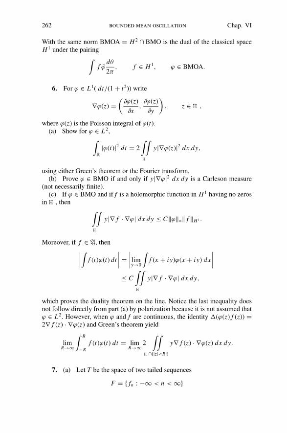
262 bounded mean oscillation Chap. VI
With the same norm BMOA = H 2 ∩ BMO is the dual of the classical spaceH 1 under the pairing
∫f ϕ
dθ
2π, f ∈ H 1, ϕ ∈ BMOA.
6. For ϕ ∈ L1( dt/(1 + t2)) write
∇ϕ(z) =(
∂ϕ(z)
∂x,∂ϕ(z)
∂y
)
, z ∈ H ,
where ϕ(z) is the Poisson integral of ϕ(t).(a) Show for ϕ ∈ L2,
∫
R
|ϕ(t)|2 dt = 2
∫∫
H
y|∇ϕ(z)|2 dx dy,
using either Green’s theorem or the Fourier transform.(b) Prove ϕ ∈ BMO if and only if y|∇ϕ|2 dx dy is a Carleson measure
(not necessarily finite).(c) If ϕ ∈ BMO and if f is a holomorphic function in H 1 having no zeros
in H , then∫∫
H
y|∇ f · ∇ϕ| dx dy ≤ C‖ϕ‖∗‖ f ‖H 1 .
Moreover, if f ∈ A, then∣∣∣∣
∫f (ı)ϕ(t) dt
∣∣∣∣ =
∣∣∣∣ lim
y→0
∫f (x + iy)ϕ(x + iy) dx
∣∣∣∣
≤ C∫∫
H
y|∇ f · ∇ϕ| dx dy,
which proves the duality theorem on the line. Notice the last inequality doesnot follow directly from part (a) by polarization because it is not assumed thatϕ ∈ L2. However, when ϕ and f are continuous, the identity �(ϕ(z) f (z)) =2∇ f (z) · ∇ϕ(z) and Green’s theorem yield
limR→∞
∫ R
−Rf (t)ϕ(t) dt = lim
R→∞2
∫∫
H ∩{|z|<R|}y∇ f (z) · ∇ϕ(z) dx dy.
7. (a) Let T be the space of two tailed sequences
F = { fn : −∞ < n < ∞}

exercises and further results 263
of measurable functions on R such that∫
supn
| fn(x)| dx = ‖F‖ < ∞.
Under this norm T is a Banach space.(b) Let T0 be the closure in T of the set of sequences F for which there
exists N = N (F) such that
fn = fN , n ≥ N ; fn = 0, n ≤ −N .
When F ∈ T0, limn→∞ fn = f exists in L1. The dual space of T0 consists ofsequences G = {gn : −∞ < n ≤ ∞} of L∞ functions with norm
‖G‖ =∥∥∥∥∥|g∞(x)| +
∞∑
−∞|gn(x)|
∥∥∥∥∥
∞
under the pairing
〈F, G〉 =∫
f∞(x)g∞(x) dx +∞∑
−∞
∫fn(x)gn(x) dx .
(c) Choose {yn : −∞ < n < ∞} such that
yn → 0 (n → ∞), yn → ∞ (n → −∞),
and
0 < yn − yn+1 ≤ min(y2n , 1).
Let S : H 1R
→ T be defined by
(S(u))n(x) = u(x, yn).
Then S maps H 1R
onto a closed subspace of T0. (Use the vertical maximalfunction
u+(x) = supy>0
|u(x, y)|.
(d) By parts (b) and (c), every bounded linear functional on H 1R
has theform
L(u) =∫
u(x)g∞(x) dx +∞∑
n=−∞
∫u(x, yn)gn(x) dx
with
1
|I |∫
I
(
|g∞(x)| +∞∑
n=−∞|gn(x)|
)
dx ≤ C‖L‖,

264 bounded mean oscillation Chap. VI
and conversely. With the duality theorem this gives the converse of Theorem1.6. If ϕ ∈ BMO, then
ϕ(t) = g∞(t) +∫
HPy(x − t)dσ (x, y),
where |σ | is a Carleson measure. Here
dσ =∞∑
−∞gn(x) dsn,
where dsn is dx on the line {y = yn}. Note that |σ | is more than a Carlesonmeasure since
|σ |(I × (0, ∞)) ≤ C |I |.This reflects the fact H 1 is determined by the vertical maximal function as wellas by the nontangential maximal function. The proof sketched above is due toFefferman (unpublished).
���(e) Carleson [1976] constructively obtained the decomposition
ϕ(t) = g∞(t) +∞∑
−∞
∫Pyn (x − t)gn(t) dt,
where |g∞| + ∑∞−∞ |gn| ∈ L∞, for each ϕ ∈ BMO.
(f) Assuming the result in (e), prove the maximal function characterizationof H 1: If u ∈ L1 ∩ L2, then
‖Hu‖1 ≤ C‖u+‖1.
(Hint: Let g ∈ L2 ∩ L∞, ‖g‖∞ = 1, and let ϕ = Hg ∈ BMO. Then∣∣∣∣
∫(Hu)g dt
∣∣∣∣ =
∣∣∣∣
∫uϕ dt
∣∣∣∣ ≤ C‖u+‖1.
The left side has supremum ‖Hu‖1.)(g) Derive the difficult half of the duality theorem from part (e).
8. Suppose f = ∑n≥0 aneinθ is in H 1. Use duality to prove∑
k>0
|a2k |2 ≤ C‖ f ‖21 (Paley)
and∑
n≥0
|an|n + 1
≤ C‖ f ‖1 (Hardy).
9. There exist BMO functions such that |∇u| dx dy is not a Carlesonmeasure. There is even a Blaschke product B(z) such that
∫∫D |B ′(z)| dx dy =
∞.

exercises and further results 265
(a) Let f (eiθ ) = ∑n≥1(1/n)ei2nθ . Then f ∈ BMO. Let An be the an-
nulus 1 − 2−n ≤ |z| ≤ 1 − 2−n−1. Then∫∫
An| f ′(z)| dx dy ≥ c/n. Writing
Re f = u1 + u2, show there is a bound harmonic function u(z) such that∫∫D |∇u| dx dy = ∞. Then F = exp(u + i u) is an H∞ function with
∫∫|F ′(z)| dx dy = ∞.
(b) If g(eiθ ) = ∑anei2n0 , then g ∈ BMO if and only if
∑ |an|2 < ∞, but∫∫ |g′(z)| dx dy < ∞ if and only if∑ |an| < ∞.
(c) If∑ |an|2 < ∞ there is F ∈ H∞ such that F(2n) = an (see Fournier
[1974]). If∑ |an|2 < ∞, but
∑ |an| = ∞ then∫∫ |F ′(z)| dx dy = ∞.
(d) There exists a Blaschke product B(z) such that∫∫
D
|B ′(z)| dx dy = ∞.
The earliest example is due to Rudin [1955b].
10. There exist f1(z) and f2(z) in H∞ such that∫
�
(| f ′1(z)| + | f ′
2(z)|) ds = ∞
for all smooth curves � in D terminating on ∂D. Consequently the mapping
z → (z, f1(z), f2(z))
embeds the unit disc into C3. The embedded manifold is bounded and it is
complete in the metric of Euclidean arc length.To construct f1 and f2, first take
ϕ(reiθ ) =∞∑
n=1
r10n
ncos(10nθ ).
Then
|∇ϕ(z)| ≥ 10n/100n on An ={9 · 10−n−1 ≤ 1−|z| ≤ 11 · 10−n−1},so that
∫
�
|∇ϕ(z)| ds = ∞
for every curve � in D which terminates on ∂D. On the other hand, ϕ(z) is thePoisson integral of ϕ(eiθ ) ∈ BMO. Write ϕ = u + v and set f1 = eu+i u, f2 =ev+i v . This example is due to Jones [1979a]. See Yang [1977] for backgroundon this problem.

266 bounded mean oscillation Chap. VI
11. An atom is a function a(x) supported on an interval I and satisfying∫
a(x) dx = 0, |a(x)| ≤ 1/|I |.
If {a j } is a sequence of atoms and if∑ |λ j | < ∞, then
f (x) =∑
λ j a j ∈ H 1R
and ‖ f ‖H 1 ≤ C∑ |λ j |. Conversely, by the duality theorem every function in
H 1R
has the above form with∑ |λ j | ≤ C‖ f ‖H 1 . See Coifman [1974] or Latter
[1978] for direct proofs of the atomic decomposition, which in turn impliesthe H 1−BMO duality.
12. (Dyadic BMO). A dyadic interval is an interval of the form ω =( j2−n, ( j + 1)2−n) with n and j integers. For ϕ ∈ L1
loc, define
‖ϕ‖d = supω
1
|ω|∫
|ϕ − ϕω| dx,
the supremum taken only over dyadic intervals. The dyadic BMO space,BMOd, consists of the functions ϕ with ‖ϕ‖d finite.
(a) BMO is a subset of BMOd, but there are functions in BMOd not inBMO.
(b) If ϕ ∈ BMOd, then ϕ ∈ BMO if and only if
|ϕω1− ϕω2
| ≤ A
whenever ω1 and ω2 are adjacent dyadic intervals of the same length. Then
C1‖ϕ‖∗ ≤ A + ‖ϕ‖d ≤ C2‖ϕ‖∗.
(c) Suppose ϕ ∈ BMOd has support [0, 1]. Then there exists a family G ofdyadic intervals ω such that
∑
ω⊂Iω∈G
|ω| ≤ C‖ϕ‖d|I |(E.1)
for every dyadic interval I, and there exist weights αω, ω ∈ G, such that |αω| ≤C‖ϕ‖d and such that
ϕ = ψ +∑
ω∈Gαωχω
with ψ ∈ L∞, ‖ψ‖∞ ≤ C‖ϕ‖d. Conversely, every function of this form is inBMOd. To prove the decomposition, mimic the proof of the John–Nirenberg
theorem. Suppose ‖ϕ‖d = 1. Take G = {I (n)j } from that proof and take αω =
ϕI (n)j
− ϕI (n−1)k
, where I (n−1)k ⊃ I (n)
j .
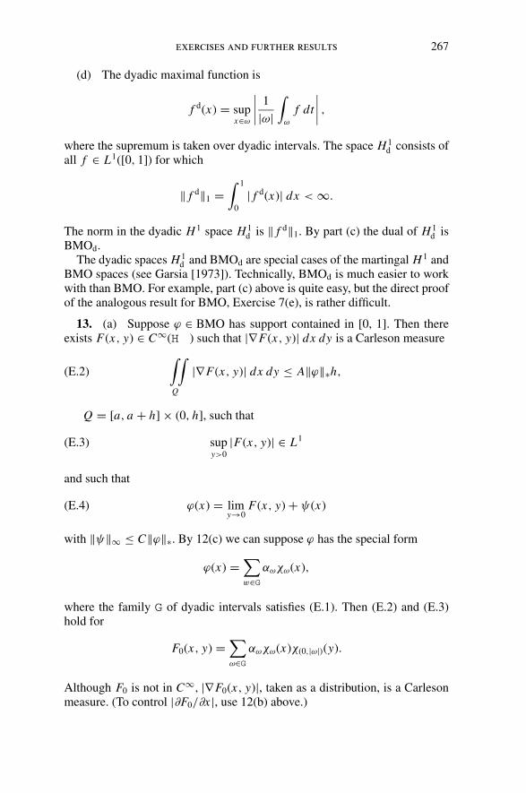
exercises and further results 267
(d) The dyadic maximal function is
f d(x) = supx∈ω
∣∣∣∣
1
|ω|∫
ω
f dt
∣∣∣∣ ,
where the supremum is taken over dyadic intervals. The space H 1d consists of
all f ∈ L1([0, 1]) for which
‖ f d‖1 =∫ 1
0
| f d(x)| dx < ∞.
The norm in the dyadic H 1 space H 1d is ‖ f d‖1. By part (c) the dual of H 1
d isBMOd.
The dyadic spaces H 1d and BMOd are special cases of the martingal H 1 and
BMO spaces (see Garsia [1973]). Technically, BMOd is much easier to workwith than BMO. For example, part (c) above is quite easy, but the direct proofof the analogous result for BMO, Exercise 7(e), is rather difficult.
13. (a) Suppose ϕ ∈ BMO has support contained in [0, 1]. Then thereexists F(x, y) ∈ C∞(H ) such that |∇F(x, y)| dx dy is a Carleson measure
∫∫
Q
|∇F(x, y)| dx dy ≤ A‖ϕ‖∗h,(E.2)
Q = [a, a + h] × (0, h], such that
supy>0
|F(x, y)| ∈ L1(E.3)
and such that
ϕ(x) = limy→0
F(x, y) + ψ(x)(E.4)
with ‖ψ‖∞ ≤ C‖ϕ‖∗. By 12(c) we can suppose ϕ has the special form
ϕ(x) =∑
w∈Gαωχω(x),
where the family G of dyadic intervals satisfies (E.1). Then (E.2) and (E.3)hold for
F0(x, y) =∑
ω∈Gαωχω(x)χ(0,|ω|)(y).
Although F0 is not in C∞, |∇F0(x, y)|, taken as a distribution, is a Carlesonmeasure. (To control |∂F0/∂x |, use 12(b) above.)

268 bounded mean oscillation Chap. VI
The smooth function F(x, y) is a mollification of F0. Let h ∈ C∞(C) satisfy
h(z) ≥ 0;∫
h dxdy = 1;
h(z) = 0, |z| > 12.
Set hn(z) = 22nh(2nz), Fn(z) = F0(z)χ{2−n<y<2−n+1}(t), and write
F(z) =∞∑
n=1
(hn ∗ Fn)(z).
Then F ∈ C∞(H ) satisfies (E.2)–(E.4) (Varopoulos [1977a]).(b) Use the result in (a) to give another proof that (H 1
R)∗ = BMO.
�14. (a) On the unit circle, the dual of VMO is H 1R
.(b) Let f ∈ BMO. Then f ∈ VMO if and only if
∫ a+h
a
∫ h
0
y|∇u(z)|2 dx dy = o(h)
uniformly in a ∈ R, where u(z) is the Poisson integral of f (t).
�15. (a) Suppose ψ ∈ BMO, ‖ψ‖∗ ≤ B0. If
supI
1
|I |∫
eψ−ψI dx = B1 < ∞,
then there are δ = δ(B0, B1) > 0 and B2 = B2(B0, B1) such that
supI
1
|I |∫
e(1+δ)(ψ−ψI ) dx ≤ B2.
The proof is a variation of the proof of the John–Nirenberg theorem. It isenough to show there is α > 1 such that for n = 1, 2, . . .
|{x ∈ I : ψ(x) − ψI > nα}| ≤ e−(1+2δ)nα|I |(E.5)
for every interval I.Take λ > 0 so that
|ψI − ψ j | ≤ 12λ(E.6)
if I ⊂ J, |J | = 2|I |, and so that
|{x ∈ I : |ψ(x) − ψI | ≥ 12λ}| ≥ 1
2|I |(E.7)
for all I. Fix an interval I0 and assume I0 = [0, 1] and ψI0= 0. For n ≥ 1, let
{In, j } be the maximal dyadic intervals inside I0 for which ψIn, j ≥ nλ. Then by(E.6)
nλ ≤ ψIn, j ≤ (n + 12)λ,

exercises and further results 269
and by (E.7) there exists En, j ⊂ I ′n, j such that |En, j | ≥ 1
2|In, j | and
ψ(x) ≥ (n − 12)λ, x ∈ En, j .
Hence for any chosen interval Im,k we have∑
n≥m
e−(m−n+1)λ∑
In, j ⊂Im,k
|In, j ||Im,k | ≤ 2
∑
n≥m
e−(m−n+1)λ|⋃
En, j |/|Im,k |
≤ C
|Im,k |∫ ∞
0
et |{x ∈ Im,k : ψ(x) − ψIm,k > t}| dt
= C
|Im,k |∫
Im,k
eψ−ψIm,k dx ≤ B1.
In particular, whenever n ≥ m∑
In, j ⊂Im,k
|In, j ||Im,k | ≤ C B1e(m−n+1)λ.(E.8)
Let s be a positive integer, s > 2. For each Im,k we have n0, m < n0 ≤ m + s,so that
e−(m−n0+1)λ∑
In0, j ⊂Im,k
|In0, j ||Im,k | ≤ C B1
s,
because otherwise (E.8) would fail. Using (E.8) to compare∑
Im+s, jto
∑In0
, j ,
we therefore obtain∑
Im+s, j ⊂Im,k
|Im+s, j ||Im,k | ≤ C B2
1
se(−s+2)λ.
Now choose s so that
C B21 e2λ/s ≤ 1
2,
set α = sλ, and δ = (log 2)/2α. Then∑
Im+s , j⊂ Im,k
|Im+s, j | ≤ e−(1+2δ)α|Im,k |,
and (E.5) follows upon iteration.This argument is due to P. Jones. There are several interesting conse-
quences.(b) If ψ ∈ BMO and if
supI
1
|I |∫
IeA/ψ−ψI | dx < ∞,(E.9)
then for some ε > 0
supI
1
|I |∫
e(A+ε)|ψ−ψI | dx < ∞.
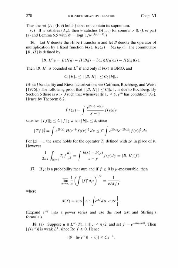
270 bounded mean oscillation Chap. VI
Thus the set {A : (E.9) holds} does not contain its supremum.(c) If w satisfies (Ap), then w satisfies (Ap−ε) for some ε > 0. (Use part
(a) and Lemma 6.5 with ψ = log((1/w)1/(p−1).)
16. Let H denote the Hilbert transform and let B denote the operator ofmultiplication by a fixed function b(x), Bg(x) = b(x)g(x). The commutator[B, H ] is defined by
[B, H ]g = B(Hg) − H (Bg) = b(x)(Hg)(x) − H (bg)(x).
Then [B, H ] is bounded on L2 if and only if b(x) ∈ BMO, and
C1‖b‖∗ ≤ ‖[B, H ]‖ ≤ C2‖b‖∗.
(Hint: Use duality and Riesz factorization; see Coifman, Rochberg, and Weiss[1976].) The following proof that ‖[B, H ]‖ ≤ C‖b‖∗ is due to Rochberg. BySection 6 there is δ > 0 such that whenever ‖b‖∗ ≤ δ, e2b has condition (A2).Hence by Theorem 6.2.
T f (x) =∫
e(b(x)−b(y))
x − yf (y)dy
satisfies ‖T f ‖2 ≤ C‖ f ‖2 when ‖b‖∗ ≤ δ, since
‖T f ‖22 =
∫e2b(x)|H (e−b f )(x)|2 dx ≤ C
∫e2b(x)e−2b(x)| f (x)|2 dx .
For |z| = 1 the same holds for the operator Tz defined with zb in place of b.However
1
2π i
∫
|z|=1
Tz fdz
z2=
∫b(x) − b(y)
x − yf (y)dy = [B, H ]( f ).
17. If μ is a probability measure and if f ≥ 0 is μ-measurable, then
limn→∞
1
n
(∫| f |ndμ
)1/n
= 1
eA( f ),
where
A( f ) = sup
{
A :
∫eA f dμ < ∞
}
.
(Expand eA f into a power series and use the root test and Stirling’sformula.)
18. (a) Suppose u ∈ L∞(T ), ‖u‖∞ ≤ π/2, and set f = e−i(u+i u). Then| f (eiθ )| is weak L1, since Re f ≥ 0. Hence
|{θ : |u(eiθ )| > λ}| ≤ Ce−λ.
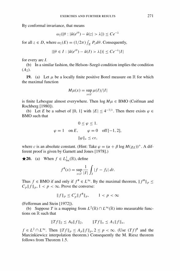
exercises and further results 271
By conformal invariance, that means
ωz({θ : |u(eiθ ) − u(z| > λ}) ≤ Ce−λ
for all z ∈ D, where ωz(E) = (1/2π )∫
E Pzdθ . Consequently,
|{θ ∈ I : |u(eiθ ) − u(I ) > λ})| ≤ Ce−λ|I |for every arc I.
(b) In a similar fashion, the Helson–Szego condition implies the condition(A2).
19. (a) Let μ be a locally finite positive Borel measure on R for whichthe maximal function
Mμ(x) = supx∈I
μ(I )/|I |
is finite Lebesgue almost everywhere. Then log Mμ ∈ BMO (Coifman andRochberg [1980]).
(b) Let E be a subset of [0, 1] with |E | ≤ 4−1/ε. Then there exists ϕ ∈BMO such that
0 ≤ ϕ ≤ 1.
ϕ = 1 on E, ϕ = 0 off [−1, 2],
‖ϕ‖∗ ≤ cε,
where c is an absolute constant. (Hint: Take ϕ = (α + β log M(χE ))+. A dif-ferent proof is given by Garnett and Jones [1978].)
�20. (a) When f ∈ L1loc(R), define
f #(x) = supx∈I
1
|I |∫
I| f − f I | dt.
Thus f ∈ BMO if and only if f # ∈ L∞. By the maximal theorem, ‖ f #‖p ≤C p‖ f ‖p, 1 < p < ∞. Prove the converse:
‖ f ‖p ≤ C ′p‖ f #‖p, 1 < p < ∞
(Fefferman and Stein [1972]).(b) Suppose T is a mapping from L2(R) ∩ L∞(R) into measurable func-
tions on R such that
‖T f ‖2 ≤ A0‖ f ‖2, ‖T f ‖∗ ≤ A1‖ f ‖∗,
f ∈ L2 ∩ L∞. Then ‖T f ‖p ≤ Ap‖ f ‖p, 2 ≤ p < ∞. (Use (T f )# and theMarcinkiewicz interpolation theorem.) Consequently the M. Riesz theoremfollows from Theorem 1.5.

272 bounded mean oscillation Chap. VI
21. A positive locally integrable weight function w(x) is said to satisfycondition (A1) if
supI
{(1
|I |∫
Iw dx
)
ess supx∈I
1
w(x)
}
< ∞.
(a) w(x) satisfies (A1, ) if and only if
Mw(x) ≤ Cw(x),
where M is the Hardy–Littlewood maximal function.(b) If w(x) satisfies (A1), then w(x) satisfies (Ap) for all p > 1.(c) w(x) satisfies (A1) if and only if the maximal function operator or the
Hilbert transform is weak-type 1–1 on L1(w dx) (Muckenhoupt [1972]; Hunt,Muckenhoupt, and Wheeden [1973]).
(d) Let ϕ = log w. Then w has (A1) if and only if
supI
1
|I |∫
Ieϕ−ϕI dx < ∞ and sup
I
(ϕI − ess inf
x∈Iϕ(x)
)< ∞.
The space of functions satisfying the latter condition is called BLO, for boundedlower oscillation. If ϕ ∈ BLO then ϕ ∈ BMO and so eεϕ has (A1) for someε > 0.
���(e) If w1 and w2 have (A1), then by Holder’s inequality w =w1w
1−p2 has (Ap). The converse is also true but quite difficult. See Jones
[1980c]. With the Helson–Szego theorem, the converse implies that if ‖v‖∞ <
1, then
Hv = u − Hu1 + Hu2,
where u ∈ L∞, ‖u j‖∞ ≤ 1, and Hu j ∈ BLO, j = 1, 2.(f) If w satisfies A1, then w1+δ satisfies A1 for some δ > 0. (Use part (b)
and Corollary 6.10.)(g) If μ is a positive Borel measure finite on compact sets such that
M(dμ) < ∞ almost everywhere and if 0 < α < 1, then (M(dμ))α has A1
(Coifman and Rochberg [1980]).��(h) For any function w(x) ≥ 0 and for any s > 1, define
As(w) = M(Mws)1/s .
Then for 1 < p < ∞∫
|H f |pw dx ≤ C p,s
∫| f |p As(w) dx
(see Cordoba and Fefferman [1976]). It then follows easily from part (a) that∫
|H f |pw dx ≤ C p
∫| f |pw dx,
1 < p < ∞ if w satisfies (A1).

exercises and further results 273
22. On the unit circle let BMOA = H 2 ∩ BMO. If f ∈ BMOA then
infg∈I ∞
‖ f − g‖∗ ≤ C infg∈L∞
‖ f − g‖∗.
�23. (a) Let f (z) be a univalent function on the unit disc. If f (z) has nozeros then log f (eiθ ) ∈ BMO. Moreover, if 0 < p < 1
2, then | f (eiθ )|p satisfies
(A2) (Baernstein [1976]; see also Cima and Petersen [1976], Cima and Schober[1976]).
(b) Let f (z) be analytic on D. Then f ∈ BMOA if and only if f =α log g′(z), where α is a constant and g is a conformal mapping from D ontoa region bounded by a rectifiable Jordan curve � satisfying
l(w1, w2) ≤ c|w1 − w2|,w1, w2 ∈ �, where l(w1, w2) is the shorter are on � joining w1 to w2 (Pom-merenke [1977]). See also Pommerenke [1978] for a similar description ofVMOA.
�24. Let E be a closed set on the Riemann sphere, ∞ ∈ E . Then everyanalytic function on D having values in C\E is in BMOA if and only if thereis r > 0 and δ > 0 such that
cap (E ∩ {|z − z0| < r}) > δ
for all z0 ∈ C\E . Here cap(S) denotes the logarithmic capacity of S (Haymanand Pommerenke [1978]; Stegenga [1979]; Baernstein [1980] has yet anotherproof).
25. The Bloch class B is the set of analytic functions f (z) on D for which
supz
(1 − |z|2)| f ′(z)| < ∞.
(a) If f (z) is analytic on D, then f ∈ B if and only if{
f
(z − w
1 − wz
)
: w ∈ D
}
is a normal family.(b) BMOA ⊂ B.(c) The function
∞∑
n=1
z2n
is in B but not in BMOA.�(d) Let f (z) be analytic on D, and let F ′(z) = f (z). Then f ∈ B if and
only if F is in the Zygmund class �∗:
F(ei(θ+h)) + F(ei(θ−h)) − 2F(eiθ ) = O(h)
274 bounded mean oscillation Chap. VI
(see Duren [1970], Zygmund [1968]). Since �∗ contains singular functions(Kahane [1969]; Piranian [1966]; Duren, Shapiro, and Shields [1966]), wehave another proof that B �= BMOA.
(e) f (z) ∈ B if and only if f (z) = α log g′(z), where α is constant andg(z) is univalent on D. (See Duren, Shapiro, and Shields [1966]; Pommerenke[1970]. Compare with 23(b).)
(f) On the other hand, B does coincide with the analytic functions in BMOof the unit disc defined by
1
πr2
∫
D∩{|z−z0|<r}| f (z) − f (z0)| dx dy ≤ C,
|z0| < 1 (Coifman, Rochberg, and Weiss [1976]).�(g) When f (z) is analytic in D, let n(w) be the number of solutions of
f (z) = w, z ∈ D. Suppose
supw0∈C
∫∫
|w−w0|<1
n(w) du dv < ∞,
w = u + iv. Then f ∈ BMOA if and only if f ∈ B, and f ∈ VMOA = H 2∩VMO if and only if f ∈ B0, defined by
lim|z|→1
(1 − |z|2)| f ′(z)| = 0
(see Pommerenke [1977]).Anderson, Clunie, and Pommerenke [1974] give an excellent overview of
the theory of Bloch functions.

VII
Interpolating Sequences
A sequence {z j } in the disc or upper half plane is an interpolating sequenceif every interpolation problem
f (z j ) = a j , j = 1, 2, . . . ,
with {a j } bounded, has solution f (z) ∈ H∞. Interpolating sequences are veryinteresting in their own right and they will play crucial roles in the analysis ofH∞ in the succeeding chapters. For example, they will be used in Chapter IXto characterize the closed algebras between H∞ and L∞ and they will be sur-prisingly important in the discussion of the maximal ideal space in Chapter X.
The notion of generations is introduced in this chapter. Similar to the stop-ping times in the proof of the John–Nirenberg theorem, generations arise natu-rally in several of the deeper proofs in this subject. They will be used frequentlyin the next chapter. Some other important techniques are also introduced. Theseinclude
(i) solving an extremal problem by a variational argument (this is done inSection 2) and
(ii) using certain ideas borrowed from harmonic analysis, such as the aver-aging process in the proof of Theorem 2.2 and the use of Khinchin’s inequalityin Section 4.
Two proofs of the interpolation theorem are given. Carleson’s original proofby duality is in Section 1, because it sheds light on the geometry of interpolat-ing sequences. Earl’s elementary proof, reminiscent of the Pick–Nevanlinnatheorem, is in Section 5.
1. Carleson’s Interpolation Theorem
Let {z j } be a sequence in the upper half plane. We want to determine whenevery interpolation problem
f (z j ) = a j , j = 1, 2, . . . ,(1.1)
275

276 interpolating sequences Chap. VII
with {a j } bounded, has a solution f (z) ∈ H∞. The sequence {z j } is called aninterpolating sequence if (1.1) has solution in H∞ for every {a j } ∈ l∞. If {z j }is an interpolating sequence, then the linear operator T : H∞ → l∞ defined byTf( j) = f (z j ) is a bounded linear mapping of H∞ onto l∞. The open mappingtheorem then gives a constant M such that (1.1) has a solution f (z) with
‖ f ‖∞ ≤ M supj
|a j | = M‖a j‖∞.
The smallest such constant M is called the constant of interpolation
M = sup‖a j ‖∞≤1
inf{‖ f ‖∞ : f ∈ H∞, f (z j ) = a j , j = 1, 2, . . . }.
Let z j and zk be distinct points in the interpolating sequence. Then thereexists f ∈ H∞ such that
f (z j ) = 0, f (zk) = 1, and ‖ f ‖∞ ≤ M.
By Schwarz’s lemma this means∣∣∣∣zk − z j
zk − z j
∣∣∣∣ = ρ(z j , zk) ≥ | f (z j )/M − f (zk)/M |
|1 − f (zk) f (z j )/M2| = 1
M,
and so∣∣∣∣zk − z j
zk − z j
∣∣∣∣ ≥ a > 0, j �= k,(1.2)
with a = 1/M . A sequence is said to be separated if (1.2) holds with constanta > 0 not depending on j and k. We have just proved that an interpolatingsequence is separated.
The above reasoning can be carried further to yield a necessary condi-tion for interpolation that will also be a sufficient condition. Fix zk , letf ∈ H∞, ‖ f ‖∞ ≤ M , interpolate the values
f (zk) = 1, f (z j ) = 0, j �= k.
Let B(k) be the Blaschke product with zeros {z j , j �= k}. Since f �= 0 thisproduct exists. Then f = B(k)g, where g ∈ H∞, and ‖g‖∞ ≤ M , so that
1 = | f (zk)| = |B(k)(zk)||g(zk)| ≤ M |B(k)(zk)|and |B(k)(zk)| ≥ 1/M . Since zk is arbitrary, we conclude that
infk
∏
j, j �=k
∣∣∣∣zk − z j
zk − z j
∣∣∣∣ ≥ δ > 0(1.3)
holds for an interpolating sequence {z j } with constant δ = 1/M . Carleson’stheorem asserts that the necessary condition (1.3) conversely implies that {z j }is an interpolating sequence.

Sect. 1 carleson’sinterpolation theorem 277
Before stating the theorem in full, let us interpret (1.3) geometrically. In theunit disc (1.3) becomes
infk
∏
j, j �=k
∣∣∣∣
zk − z j
1 − z j zk
∣∣∣∣ ≥ δ > 0.(1.4)
Let B(z) be the full Blaschke product
B(z) =∞∏
j=1
−z j
|z j |(
z − z j
1 − z j z
)
.
If we view zk as the origin by taking w = (z − zk)/(1 − zk z) as the coordinatefunction on the disc, then the zeros of B are
w j = z j − zk
1 − zk z j, j = 1, 2, . . . ,
and (1.4) holds if and only if for all k∏
j, j �=k
|w j | ≥ δ.
Since 1 − |w| ≤ log 1/|w|, this gives∑
j
(1 − |w j |) ≤ 1 + log 1/δ,(1.5)
and (1.4) holds if and only if the Blaschke sum (1.5) has a bound that doesnot depend on which point zk is regarded as the origin. This fact, of course,reflects the conformal invariance of the interpolation problem (1.1). With theidentity
1 −∣∣∣∣
z j − zk
1 − zk z j
∣∣∣∣
2
= (1 − |zk |2)(1 − |z j |2)
|1 − zk z j |2 ,
from Section 1 of Chapter I, (1.5) gives
supk
∑
j
(1 − |zk |2)
|1 − zk z j |2 (1 − |z j |2) ≤ C(δ).
If this supremum were taken over all points in the disc instead of only oversequence points, we should have
supz0∈D
∑
j
(1 − |z0|2)
|1 − z0z j |2 (1 − |z j |2) ≤ C ′(δ).(1.6)
By the conformally invariant description of Carleson measures (Chapter VI,Lemma 3.3), (1.6) holds if and only if the measure
∑(1 − |z j |)δz j
278 interpolating sequences Chap. VII
is a Carleson measure on the disc. Now it is not very hard to see that (1.4) doesimply (1.6), and that conversely, if the sequence is separated, (1.6) implies (1.4).(The complete arguments are given below during the proof of the theorem.)This discussion does not prove the theorem, but it should clarify the connectionbetween Carleson measures and interpolation. Historically it was with theinterpolation theorem that Carleson measures first arose.
To state the theorem we return to the half plane.
Theorem 1.1. If {z j } is a sequence in the upper half plane, then the followingconditions are equivalent:
(a) The sequence is an interpolating sequence: Every interpolation problem
f (z j ) = a j , j = 1, 2, . . . ,
with {a j } ∈ l∞ has solution f ∈ H∞.(b) There is δ > 0 such that
∏
j, j �=k
∣∣∣∣zk − z j
zk − z j
∣∣∣∣ ≥ δ, k = 1, 2, . . . .(1.3)
(c) The points z j are separated,
ρ(z j , zk) =∣∣∣∣z j − zk
z j − zk
∣∣∣∣ ≥ a > 0, j �= k,
and there is a constant A such that for every square Q = {x0 ≤ x ≤ x0 +�(Q), 0 < y ≤ �(Q)},
∑
z j ∈Q
y j ≤ A�(Q).(1.7)
The constant δ in (1.3) and the constant of interpolation
M = sup‖a j ‖∞≤1
inf{‖ f ‖∞ : f (z j ) = a j , j = 1, 2, . . . , f ∈ H∞}
are related by the inequalities
1
δ≤ M ≤ c
δ
(
1 + log1
δ
)
,(1.8)
in which c is some absolute constant.
Except for the value of the numerical constant c, the upper bound given forM in (1.8) is sharp. An example illustrating this will be given after the proof.
Of course, (1.7) says that∑
y jδz j is a Carleson measure. Condition (c),being more geometric, is in some ways more useful than (b). Before turningto the proof we consider two examples. First, suppose the points z j lie ona horizontal line {y j = y > 0}. Then (1.7) holds as soon as the points areseparated. So a horizontal sequence is an interpolating sequence if and only ifit is separated. This fact can also be derived from (1.3) without much difficulty.
Sect. 1 carleson’sinterpolation theorem 279
For the second example, suppose the points z j lie on the vertical line x = 0.Then (1.7) holds if and only if
∑
y j ≤yk
y j ≤ Ayk, k = 1, 2, . . . ,
This condition is satisfied if the points are separated. If the y j are boundedabove and if the points are indexed so that y j+1 < y j , then this condition holdsif and only if the points tend to the boundary exponentially:
y j+1/y j ≤ α < 1.
Thus a vertical sequence is an interpolating sequence if and only if it is sep-arated. Of course, not every separated sequence satisfies (1.7). A sequencehaving only (1.2) need not be a Blaschke sequence; it could have subsequencesconverging nontangentially to each point on the line.
Proof of Theorem 1.1. We have already seen that (a) implies (b), along withthe estimate M ≥ 1/δ.
There are two remaining steps in the proof. First we show that (b) and (c)are equivalent. This is really only a matter of comparing infinite products toinfinite sums. Second, we must show that (b) and (c) together imply (a). Thiswill be done with a dual extremal problem.
To show that (b) and (c) are equivalent we need an elementary lemma.
Lemma 1.2. Let B(z) be the Blaschke product in the upper half plane withzeros {z j }. Then
− log |B(z)|2 ≥∑
j
4yy j
|z − z j |2 , z = x + iy.(1.9)
Conversely, if
infj
ρ(z, z j ) = infj
∣∣∣∣z − z j
z − z j
∣∣∣∣ = a > 0,
then
− log |B(z)|2 ≤(
1 + 2 log1
a
) ∑ 4yy j
|z − z j |2 .(1.10)
Proof. The inequality − log t ≥ 1 − t, t > 0, gives
− log
∣∣∣∣z − z j
z − z j
∣∣∣∣
2
≥ 1 −∣∣∣∣z − z j
z − z j
∣∣∣∣
2
= 4yy j
|z − z j |2 .
Summing now gives (1.9). The reverse inequality,
− log t ≤ −2 log a
1 − a2(1 − t) ≤
(
1 + 2 log1
a
)
(1 − t),
is valid for a2 < t < 1, and in a similar fashion it gives (1.10).

280 interpolating sequences Chap. VII
Now suppose (c) holds. Then (1.7) and (3.8) of Chapter VI give
∑
j
4yk y j
|zk − z j |2 =∑
j
4yk y j
|z j − zk |2 ≤ C ′, k = 1, 2, . . . .(1.11)
For convenience we directly derive (1.11) from (1.7), essentially repeating theproof of (3.8) of Chapter VI. Fix zk = xk + iyk and let Sn = {z ∈ H : |z −xk | ≤ 2n yk}, n = 0, 1, 2, . . . . By (1.7),
∑Sn
y j ≤ c2n+1 yk . When z j ∈ S0, we
have |z j − zk |2 ≥ y2k , and when z j ∈ Sn\Sn−1, n ≥ 1, we have |z j − zk |2 ≥
22n−2 y2k . Consequently,
∑
j
4yk y j
|z j − zk |2 ≤ 4∑
z j ∈S0
y j
yk+ 16
∞∑
n=1
(∑
z j ∈Sn\Sn−1
y j
22n yk
)
≤ 8A + 32A∞∑
1
2−n = A′.
Since inf j, j �=k |(zk − z j )/(zk − z j )| ≥ a, we can now use (1.10) on theBlaschke product B(k) with zeros {z j : j �= k} to obtain
∏
j, j �=k
∣∣∣∣zk − z j
zk − z j
∣∣∣∣ ≥ δ = δ(a, A).
Hence (c) implies (b).Now suppose (b) holds; that is, suppose
infk
∏
j, j �=k
∣∣∣∣zk − z j
zk − z j
∣∣∣∣ ≥ δ.
Then trivially∣∣∣∣zk − z j
zk − z j
∣∣∣∣ ≥ δ, j �= k,
and the points are separated. Using (1.9) with the Blaschke product B(k)(z)formed by deleting one zero zk , we obtain
∑
j, j �=k
4y j yk
|zk − z j |2 ≤ 2 log1
δ.
Consider a square
Q = {x0 ≤ x ≤ x0 + �(Q), 0 < y ≤ �(Q)}.We first treat the special case in which the top half
T (Q) = {z ∈ Q : y > �(Q)/2}
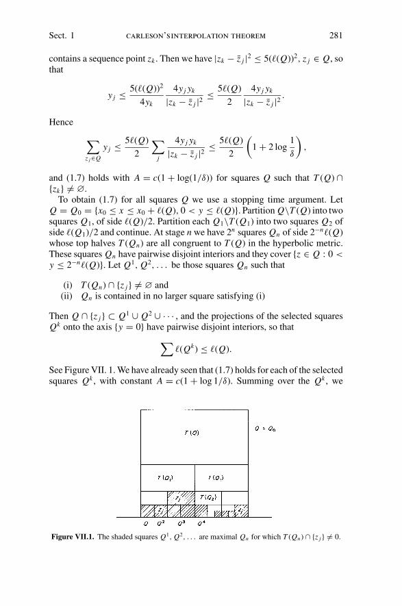
Sect. 1 carleson’sinterpolation theorem 281
contains a sequence point zk . Then we have |zk − z j |2 ≤ 5(�(Q))2, z j ∈ Q, sothat
y j ≤ 5(�(Q))2
4yk
4y j yk
|zk − z j |2 ≤ 5�(Q)
2
4y j yk
|zk − z j |2 .
Hence
∑
z j ∈Q
y j ≤ 5�(Q)
2
∑
j
4y j yk
|zk − z j |2 ≤ 5�(Q)
2
(
1 + 2 log1
δ
)
,
and (1.7) holds with A = c(1 + log(1/δ)) for squares Q such that T (Q) ∩{zk} �= ∅.
To obtain (1.7) for all squares Q we use a stopping time argument. LetQ = Q0 = {x0 ≤ x ≤ x0 + �(Q), 0 < y ≤ �(Q)}. Partition Q\T (Q) into twosquares Q1, of side �(Q)/2. Partition each Q1\T (Q1) into two squares Q2 ofside �(Q1)/2 and continue. At stage n we have 2n squares Qn of side 2−n�(Q)whose top halves T (Qn) are all congruent to T (Q) in the hyperbolic metric.These squares Qn have pairwise disjoint interiors and they cover {z ∈ Q : 0 <
y ≤ 2−n�(Q)}. Let Q1, Q2, . . . be those squares Qn such that
(i) T (Qn) ∩ {z j } �= ∅ and(ii) Qn is contained in no larger square satisfying (i)
Then Q ∩ {z j } ⊂ Q1 ∪ Q2 ∪ · · · , and the projections of the selected squaresQk onto the axis {y = 0} have pairwise disjoint interiors, so that
∑�(Qk) ≤ �(Q).
See Figure VII. 1. We have already seen that (1.7) holds for each of the selectedsquares Qk , with constant A = c(1 + log 1/δ). Summing over the Qk , we
Figure VII.1. The shaded squares Q1, Q2, . . . are maximal Qn for which T (Qn) ∩ {z j } �= 0.

282 interpolating sequences Chap. VII
obtain
∑
z j ∈Q
y j ≤ c
(
1 + log1
δ
)
�(Q),
which proves (1.7) in general. Hence (b) implies (c).In order to get the sharp inequality (1.8) we must make use of the fact that
the constant A in (1.7) has the form
A ≤ c
(
1 + log1
δ
)
.(1.12)
Now we must show that (b) and (c) imply (a). Let {a j } ∈ l∞, |a j | ≤ 1, andconsider the finite problem
f (z j ) = a j , 1 ≤ j ≤ n.(1.13)
Since the points are distinct it is trivial that the finite problem (1.13) has asolution f (z) ∈ H∞. For example, take f (z) = p(z)/(z + i)n , where p(z) isa polynomial of degree n. Let
Mn({a j }) = inf{‖ f ‖∞ : f ∈ H∞, f (z j ) = a j , 1 ≤ j ≤ n},and let
Mn = sup‖a j ‖∞≤1
Mn({a j }).
By normal families the theorem will be proved and inequality (1.8) will beestablished if we show that
limn
Mn ≤ c
δ
(
1 + log1
δ
)
.
Let
Bn(z) =n∏
j=1
z − z j
z − z j.
For fixed {a j } let f0 ∈ H∞ be a solution of (1.13). Then
Mn({a j }) = inf{‖ f0 + Bng‖∞ : g ∈ H∞} = inf{‖ f0 Bn + g‖∞ : g ∈ H∞}.Since
H∞ ={
g ∈ L∞ :
∫gG dx = 0 for all G ∈ H 1
}
,
duality now gives
Mn({a j }) = sup
{∣∣∣∣
∫f0 BnG dx
∣∣∣∣ : G ∈ H 1, ‖G‖1 ≤ 1
}
.
Sect. 1 carleson’sinterpolation theorem 283
Now by Cauchy’s theorem we have, for G ∈ H 1,
∫
�
f0 BnG dx =∫
�
f0(x)G(x)
Bn(x)dx = 2π i
n∑
j=1
f0(z j )G(z j )
B ′n(z j )
.
(In the contour integral the large semicircles tending to infinity are disregardedbecause we can take G(z) in the H 1 norm dense set of functions G1(z) with|G1(z)| = O(|z|−2)). Since f0(z j ) = a j , j = 1, 2, . . . , n, this gives
Mn = sup‖a j ‖∞≤1
sup
{
2π
∣∣∣∣∣
n∑
j=1
a j G(z j )
B ′n(z j )
∣∣∣∣∣
: G ∈ H 1, ‖G‖1 ≤ 1
}
.
For fixed G(z), the {a j } can be chosen so that |a j | = 1 and so that
a j G(z j )/B ′n(z j ) ≥ 0.
We therefore have
Mn = sup
{
2π
n∑
j=1
|G(z j )||B ′
n(z j )| : G ∈ H 1, ‖G‖1 ≤ 1
}
.(1.14)
Now
B ′n(z j ) = −i
2y j
n∏
k=1k �= j
(z j − zk
z j − zk
)
,
and so (b) implies that
|B ′n(z j )| ≥ δ/2y j .
Hence
Mn ≤ 4π
δsup
{n∑
j=1
y j |G(z j )| : G ∈ H 1, ‖G‖1 ≤ 1
}
.
By condition (c), the measure∑
y jδz j is a Carleson measure, and so by The-orem II.3.9
sup
{n∑
j=1
y j |G(z j )| : G ∈ H 1, ‖G‖1 ≤ 1
}
≤ C A,
where A is the constant from (1.7). Consequently
limn→∞ Mn ≤ 4πC A/δ
and (a) is proved.
284 interpolating sequences Chap. VII
We have now shown that (a)–(c) are equivalent. Moreover, using the estimate(1.12) of the constant A in (1.7), we get
M = limn
Mn ≤ c
δ
(
1 + log1
δ
)
and (1.8) is proved.Here is an example to show that (1.8) is sharp. Let ω = e2π i/N be a primitive
Nth root of unity. In the disc take the finite sequence
z j = rω j , j = 1, 2, . . . , N .
The two parameters N and r < 1 will be fixed later. The Blaschke product withzeros z j is
B(z) = zN − r N
1 − r N zN.
From (1.4) we have
δ = inf(1 − |z j |2)|B ′(z j )| = Nr N−1 1 − r2
1 − r2N.
Consider the interpolation problem
f (z j ) = a j = ω− j .
By Theorem I.2.4 or by IV.1.8 this finite problem has a unique interpolatingfunction f (z) of minimal norm and
f (z) = m B1(z),
where B1 is a Blaschke product with at most N − 1 zeros. Since
z j+1 = ωz j , a j+1 = ω−1a j ,
the uniqueness implies that
f (z) = ω f (ωz).
Hence the zero set of B1(z) is invariant under multiplication by ω. As there areat most N − 1 zeros, all the zeros are at z = 0, and
f (z) = mz p
with p ≤ N − 1. A simple calculation then gives
f (z) = r1−N zN−1.
Let r → 1 and N → ∞ in such a way that m = r1−N is fixed. Then
δ = Nm1 − r2
m2 − r2and lim
N→∞N (1 − r2) = 2 log m,
Sect. 2 the linear operator of interpolation 285
so that for large N
δ ≥ (log m)/m.
Consequently there exist finite interpolating sequences such that
M ≥ m ≥ 1
δlog
1
δ.
2. The Linear Operator of Interpolation
Let {z j } be an interpolating sequence in the upper half plane. In this sectionwe prove that there exist interpolating functions that depend linearly on theinterpolated values {a j }. This useful result is obtained through a nonlinearextremal problem.
Theorem 2.1. Let {z j } be an interpolating sequence in the upper half plane,and let
M = sup‖a j ‖≤1
inf{‖ f ‖∞ : f ∈ H∞, f (z j ) = a j , j = 1, 2, . . . }
be the constant of interpolation. Then there are functions f j (z) ∈ H∞ suchthat
f j (z j ) = 1, f j (zk) = 0, k �= j,(2.1)
and∑
j
| f j (z)| ≤ M.(2.2)
Before proving this theorem let us give two applications. Suppose {a j } ∈ l∞.By (2.2) the function
f (z) =∑
j
a j f j (z)(2.3)
is in H∞, and by (2.1) this function interpolates
f (z j ) = a j , j = 1, 2, . . . .
Thus (2.3) produces interpolating functions that depend linearly on {a j }. With(2.3) we have defined a linear operator S : l∞ → H∞ by S({a j }) = ∑
a j f j ,and S is a linear operator of interpolation, which simply means that S is linearand that
S({a j })(zk) = ak, k = 1, 2, 3, . . . .(2.4)
By (2.2) the operator S is bounded and ‖S‖ ≤ M . Since the constant M in (2.2)is the constant of interpolation, we actually have ‖S‖ = M . Now any operator,

286 interpolating sequences Chap. VII
linear or not, that satisfies (2.4) must have
sup‖a j ‖∞≤1
‖S({a j })‖∞ ≥ M
because M is the constant of interpolation. Thus (2.3) solves all interpolationproblems (1.1) simultaneously with a linear operator whose norm is as smallas possible. The inequalities
‖a j‖∞ ≤ ‖S({a j })‖∞ ≤ M‖a j‖∞
show that the range S(l∞) is a closed subspace of H∞ and that, as a Banachspace, S(l∞) is isomorphic to l∞. The linear operator P : H∞ → S(l∞) de-fined by
Pg =∑
j
g(z j ) f j
is a bounded operator from H∞ onto S(l∞) such that P2 = P . By definition,this means that P is a projection and that P(H∞) = S(l∞) is a complementedsubspace of H∞. (The complement is the kernel of P.) Hence Theorem 2.1shows that H∞ contains a closed complemented subspace isomorphic to l∞.
The second application concerns interpolation by bounded analytic functionshaving values in a Banach space. A function f (z) from an open set in the planeto a Banach space Y is analytic if f (z) can be locally represented as a sumof a power series that has coefficients in Y and that is absolutely convergent.Equivalently, for each y∗ ∈ Y ∗, the complex valued function z → 〈y∗, f (z)〉 isanalytic. To quote Hoffman [1962a], “Any two reasonable-sounding definitionsof an analytic function with values in a Banach space are equivalent.”
Let {z j } be an interpolating sequence in the upper half plane. Let Y be aBanach space and let {a j } be a bounded sequence in Y,
supj
‖a j‖Y < ∞.
If { f j } is the sequence of scalar-valued functions given by Theorem 2.1, then
f (z) =∑
f j (z)a j
is an analytic function on the upper half plane with values in Y. By (2.1), f (z)solves the interpolation problem
f (z j ) = a j , j = 1, 2, . . . ,
and by (2.2), f (z) is bounded:
‖ f ‖ = supz
‖ f (z)‖Y ≤ supz
∑| f j (z)|‖a j‖Y ≤ M sup
j‖a j‖Y .(2.5)
We conclude that {z j } is also an interpolating sequence for the Y-valuedbounded analytic functions. Conversely, it is trivial that an interpolating se-quence for Y-valued H∞ functions is an interpolating sequence for scalar
Sect. 2 the linear operator of interpolation 287
functions. Just interpolate scalar multiples of a fixed vector in Y. Inequality(2.5) shows that the constant of interpolation is the same in the Banach spacecase as it is in the scalar case.
Proof of Theorem 2.1. For λ1, λ2, . . . , λn ≥ 0, define the functional
ϕ(G) =n∑
j=1
λ j |G(z j )|, G ∈ H 1,
and consider the extremal problem
mn = mn({λ j }) = sup{ϕ(G) : G ∈ H 1, ‖G‖1 ≤ 1}.(2.6)
This is a nonlinear problem to which the method of Chapter IV does not apply.But we can use an older method, usually referred to as a variational argument.There clearly exists an extremal function G0 for (2.6), and G0 must be an outerfunction,
G0 = eU0+iU0 .
Let u(x) be a real compactly supported continuous function. Then for t ∈ �
Gt = G0etu+i t u
is another H 1 function and
mn‖Gt‖1 ≥ ϕ(Gt ),
with equality at t = 0. Write this inequality as mn‖Gt‖1 − ϕ(Gt ) ≥ 0 anddifferentiate with respect to t at t = 0. We obtain
mn
∫|G0(x)|u(x) dx =
n∑
j=1
λ j |G0(z j )|u(z j )
=∫ ∑ λ j |G0(z j )|
π
y j
(x j − x)2 + y2j
u(x) dx .
Because u(x) is arbitrary, this means
mn|G0(x)| = 1
π
∑
j
λ j |G0(z j )|y j
(x j − x)2 + y2j
and we have almost everywhere
mn = 1
π
n∑
j=1
|G0(z j )||G0(x)|
λ j y j
(x − x j )2 + y2j
.(2.7)
Now let
Bn(z) =n∏
j=1
z − z j
z − z j

288 interpolating sequences Chap. VII
and put λ j = 2π |B ′n(z j )|−1 in (2.6). Then (2.6) is the same as the extremal
problem (1.14) and
mn = Mn = sup|a j |≤1
inf{‖ f ‖∞ : f ∈ H∞, f (z j ) = a j , 1 ≤ j ≤ n}.
From (2.7) we now have
Mn =n∑
j=1
|G0(z j )||G0(x)|
1
|B ′n(z j )|
2y j
|x − z j |2(2.8)
almost everywhere. Now set
f (n)j (z) = G0(z j )
G0(z)
Bn(z)
B ′n(z j )
2iy j
(z − z j )(z − z j ), j = 1, 2, . . . , n.
Then by (2.8),∑
| f (n)j (x)| = Mn
almost everywhere. The functions f (n)j are in N+, because G0 is outer, and so
∑| f (n)
j (z)| ≤∑ ∫
| f (n)j (t)|Pz(t) dt ≤ Mn.
Clearly f (n)j (zk) = 0, k �= j, 1 ≤ k ≤ n. Calculating B ′
n(z j ) explicitly shows
that f (n)j (z j ) = 1. Taking a limit as n → ∞, we obtain functions f j in H∞, j =
1, 2, . . . that satisfy (2.1) and (2.2).
Generally, it is not always the case that a linear operator of extension exists.However, there is an elegant result from uniform algebra theory that impliesTheorem 2.1 with a poorer bound on
∑ | f j (z)|. The idea comes from harmonicanalysis.
Theorem 2.2. Let A be a uniform algebra on a compact space X. Let{p1, p2, . . . , pn} be a finite set of points in X and let
M = sup‖a j ‖∞≤1
inf{‖g‖ : g ∈ A, g(p j ) = a j , j = 1, 2, . . . , n}.
For any ε > 0 there are functions f1, f2, . . . , fn in A such that
f j (p j ) = 1, f j (pk) = 0, k �= j(2.9)
and such that
supx∈X
n∑
j=1
| f j (x)| ≤ M2 + ε.
Sect. 3 generations 289
By normal families, Theorem 2.2 implies Theorem 2.1 except that the sharpinequality (2.2) is replaced by the weaker
∞∑
j=1
| f j (z)| ≤ M2.
For a general uniform algebra it is not possible to extend Theorem 2.2 to infiniteinterpolating sequences.
Proof. Let ω = e2π i/n be a primitive nth root of unity. Let g j (x) ∈ A, ‖g j‖ ≤M + δ, where δ > 0, interpolate
g j (pk) = ω jk, k = 1, 2, . . . , n.
Set
f j (x) =(
1
n
n∑
k=1
ω− jk gk(x)
)2
.
Then f j ∈ A and f j (p j ) = 1. Since∑n
k=1 ω(l− j)k = 0 for l �= j, f j (pl) = 0 ifl �= j . Moreover
n∑
j=1
| f j (x)| = 1
n2
n∑
j=1
(n∑
k=1
ω− jk gk(x)n∑
l=1
ω jl gl(x)
)
= 1
n2
n∑
k=1
n∑
l=1
gk(x)gl(x)n∑
j=1
ω(l−k) j
= 1
n2
n∑
k=1
n|gk(x)|2 ≤ (M + δ)2 ≤ M2 + ε
if δ is small.
3. Generations
Let {z j } be a sequence in the upper half plane. We assume that {z j } isseparated:
|z j − zk | ≥ by j , k �= j,(3.1)
with b > 0. This condition (3.1) is clearly equivalent to (1.2), but (3.1) isslightly more convenient for our present purpose. Then the condition
∑
z j ∈Q
y j ≤ A�(Q)(3.2)
holds for every square Q = {x0 ≤ x ≤ x0 + �(Q), 0 < y ≤ �(Q)}, with con-stant A independent of Q, if and only if {z j } is an interpolating sequence.
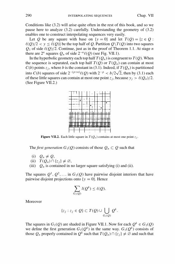
290 interpolating sequences Chap. VII
Conditions like (3.2) will arise quite often in the rest of this book, and so wepause here to analyze (3.2) carefully. Understanding the geometry of (3.2)enables one to construct interpolating sequences very easily.
Let Q be any square with base on {y = 0} and let T (Q) = {z ∈ Q :�(Q)/2 < y ≤ �(Q)} be the top half of Q. Partition Q\T (Q) into two squaresQ1 of side �(Q)/2. Continue, just as in the proof of Theorem 1.1. At stage nthere are 2n squares Qn of side 2−n�(Q) (see Fig. VII.1).
In the hyperbolic geometry each top half T (Qn) is congruent to T (Q). Whenthe sequence is separated, each top half T (Q) or T (Qn) can contain at mostC(b) points z j , where b is the constant in (3.1). Indeed, if T (Qn) is partitioned
into C(b) squares of side 2−(p+n)�(Q) with 2−p < b/2√
2, then by (3.1) eachof these little squares can contain at most one point z j , because y j > �(Qn)/2.(See Figure VII.2.)
Figure VII.2. Each little square in T (Qn) contains at most one point z j .
The first generation G1(Q) consists of those Qn ⊂ Q such that
(i) Qn �= Q,(ii) T (Qn) ∩ {z j } �= ∅,
(iii) Qn is contained in no larger square satisfying (i) and (ii).
The squares Q1, Q2, . . . in G1(Q) have pairwise disjoint interiors that havepairwise disjoint projections onto {y = 0}. Hence
∑
G1(Q)
l(Qk) ≤ �(Q).
Moreover
{z j : z j ∈ Q} ⊂ T (Q) ∪⋃
G1(Q)
Qk .
The squares in G1(Q) are shaded in Figure VII.1. Now for each Qk ∈ G1(Q)we define the first generation G1(Qk) in the same way. G1(Qk) consists ofthose Qn properly contained in Qk such that T (Qn) ∩ {z j } �= ∅ and such that
Sect. 3 generations 291
Qn is maximal. The second generation is
G2(Q) =⋃
G1(Q)
G1(Qk).
The later generations G3(Q), G4(Q), . . . are defined recursively:
G p+1 =⋃
G p(Q)
G1(Qk).
If z j ∈ Q, then either z j ∈ T (Q), or z j ∈ T (Qk) for some square Qk in somegeneration G p(Q). In the second case y j is comparable to �(Qk). Write
tp =∑
G p(Q)
�(Qk).
From the definitions it is clear that
tp+1 ≤ tp ≤ �(Q).
Theorem 3.1. Assume {z j } is a sequence of points in the upper half planesatisfying the separation condition (3.1). Then {z j } is an interpolating sequenceif and only if, for any ε > 0, there is q such that for any square Q
tq =∑
G p(Q)
�(Qk) ≤ ε�(Q).(3.3)
The smallest constant q such that (3.3) holds is related to the constant A in(3.2) by
q ≤ 1 + 2A/ε and A ≤ C(b, ε, q),
where b is the constant in (3.1).
Proof. For z j ∈ T (Qn), we have
y j ≤ �(Qn) ≤ 2y j .
Each T (Qn) or T (Q) contains at most C(b) points z j and if Qk ∈ G p(Q), thenT (Qk) contains at least one point z j . Hence
∞∑
p=1
tp ≤ 2∑
z j ∈Q
y j ≤ 2C(b)
(
�(Q) +∞∑
p=1
tp
)
.
If interpolation holds, then we have (3.2), and so
qtq ≤q∑
p=1
tp ≤ 2A�(Q).

292 interpolating sequences Chap. VII
This gives (3.3) if q ≥ 2A/ε. Conversely, if (3.3) holds for all squares, thenthe recursive definition of the generations gives
tp+q ≤ εtp, p = 1, 2, . . . ,
so that
Nq+q∑
Nq+1
tp ≤ εNq∑
1
tp ≤ qεN �(Q).
Therefore
∑
z j ∈Qy j ≤ C(b)
(
�(Q) +∞∑
N=0
qεN �(Q)
)
≤ C(b)
(
1 + q
1 − ε
)
�(Q),
and we have (3.2).
4. Harmonic Interpolation
The proof we shall give of the next theorem requires a randomization tech-nique that has been very useful in many other areas of analysis. Thus wepause briefly to discuss Khinchin’s inequality before turning to the theoremon harmonic interpolating sequences.
Given finitely many complex numbers α1, α2, . . . , αn , consider the 2n pos-sible sums
n∑
j=1
±α j
obtained as the plus–minus signs vary in the 2n possible ways. Let p > 0.Khinchin’s inequality is an estimate on the expectation
E
(∣∣∣∣∣
n∑
j=1
±α j
∣∣∣∣∣
p)
.
The expectation is the average value of | ∑ ±α j |p over the 2n choices of sign,To be precise, let � be the set of 2n points
ω = (ω1, ω2, . . . , ωn),
where ω j = ±1. Define the probability μ on � so that each point ω has prob-ability 2−n . Also define
X (ω) =n∑
j=1
α jω j .
Sect. 4 harmonic interpolation 293
Then X (ω) is a more rigorous expression for∑ ±α j , and by definition
E
(∣∣∣∣∣
n∑
j=1
±α j
∣∣∣∣∣
p)
= 1
2n
∑
ω∈�
|X (ω)|p =∫
�
|X (ω)|pdμ.
The following lemma is called Khinchin’s inequality.
Lemma 4.1. If 0 < p < ∞, then(
E
(∣∣∣∣∣
n∑
j=1
±α j
∣∣∣∣∣
p))1/p
≤ C p
(∑|α j |2
)1/2
,(4.1)
where C p is a constant that does not depend on n.
The important thing in (4.1) is that C p does not increase as n increases.We prove Lemma 4.1 only in the easy case p ≤ 2 because we need only usethat case here. (See Zygmund [1968] for the complete proof and for otherapplications.)
Proof for p≤ 2. The case p ≤ 2 is easier because it is only Holder’s inequalityin disguise. Let X j (ω) = ω j , j = 1, 2, . . . , n. Then |X2
j (ω)| = 1, and for j �=k,E(X j Xk) = 0 because X j Xk takes each value ±1 with probability 1
2. This
means that {X1, X2, . . . , Xn} are orthonormal in L2(μ). Since X = α1 X1 +α2 X2 + · · · + αn Xn and since p ≤ 2, Holder’s inequality gives
(
E
∣∣∣∣∣
n∑
j=1
±α j
∣∣∣∣∣
p)1/p
=(∫
|X (ω)|p dμ
)1/p
≤(∫
|X (ω)|2 dμ
)1/2
=(
n∑
j=1
|α j |2)1/2
.
This proves (4.1) with C p = 1 when p ≤ 2.
Now let {z j } be a sequence in the upper half plane. We say that {z j } is aharmonic interpolating sequence if every interpolation problem
u(z j ) = a j , j = 1, 2, . . . , {a j } ∈ l∞,(4.2)
can be solved with a bounded harmonic function u(z). Obviously every H∞interpolating sequence is a harmonic interpolating sequence. Our theorem isthe converse.
Theorem 4.2. If {z j } is a harmonic interpolating sequence, then {z j } is aninterpolating sequence for H∞.
Proof. Since every bounded harmonic function is the Poisson integral of anL∞ function, (4.2) holds if and only if there is an L∞ solution to every moment
294 interpolating sequences Chap. VII
problem∫
u(t)Pj (t) dt = a j , j = 1, 2, . . . , {a j } ∈ l∞,(4.3)
where
Pj (t) = 1
πy j
1
1 + ((t − x j )/y j )2
is the Poisson kernel for z j . We show that the geometric conditions (1.2) and(1.7) hold if every moment problem (4.3) can be solved with u ∈ L∞. ByTheorem 1.1 this will mean that {z j } is an H∞ interpolating sequence.
To get started we need an inequality. Consider the linear operator T : L∞ →l∞ defined by
T u( j) = u(z j ) =∫
u(t)Pj (t) dt.
Since ‖Pj‖1 = 1, this operator is bounded. We are assuming T maps L∞onto l∞. By the open mapping theorem, there is a constant M such that everyproblem (4.3) has solution u such that
‖u‖∞ ≤ M supj
|a j |.(4.4)
The inequality we need is∑
|λ j | ≤ M‖∑
λ j Pj‖1,(4.5)
which is the dual formulation of (4.4). The equivalence of (4.4) and (4.5)follows from the fact that a linear operator has closed range if and only if itsadjoint has closed range (Dunford and Schwartz [1958]). (T is the adjoint ofan operator from l1 to L1.) But (4.5) is also easily derived directly from (4.4).Given λ1, λ2, . . . , λn , pick u ∈ L∞, ‖u‖∞ ≤ M , solving
∫u(t)Pj (t) dt = λ j/|λ j |, j = 1, 2, . . . , n.
Then
n∑
j=1
|λ j | =∣∣∣∣∣
∫u
n∑
j=1
λ j Pj dt
∣∣∣∣∣≤ ‖u‖∞
∥∥∥∥∥
n∑
j=1
λ j Pj
∥∥∥∥∥
1
,
and (4.5) is proved.If j �= k, then (4.5) gives ‖Pj − Pk‖1 ≥ 2/M . By Harnack’s inequality, for
example, this means that
|z j − zk |/y j ≥ b(M) > 0, j �= k,
and (1.2) holds for the sequence {z j }.

Sect. 4 harmonic interpolation 295
The proof of (1.7) uses Khinchin’s inequality. Let Q be a square {x ∈ I, 0 <
y ≤ |I |}. Reindexing, let z1, z2, . . . , zn be finitely many points in the sequenceand in the square Q. Set λ j = ±y j , j = 1, 2, . . . , n. Then by (4.5)
n∑
j=1
y j ≤ M∫ ∣
∣∣∣∣
n∑
j=1
±yi Pj (t)
∣∣∣∣∣dt.
Taking the expectation for each t ∈ �, we get from (4.1)
n∑
j=1
y j ≤ M∫ (
n∑
j=1
y2j P2
j (t)
)1/2
dt.(4.6)
Let I be that interval concentric with I but having length | I | = 3|I |. The rightside of (4.6) is
M∫
I
(n∑
j=1
y2j P2
j
)1/2
dt + M∫
�\ I
(n∑
j=1
y2j P2
j
)1/2
dt.
For the first integral the Cauchy–Schwarz inequality gives the bound
M | I |1/2
(∫
I
∑y2
j P2j dt
)1/2
≤ cM |I |1/2
(n∑
j=1
y j
)1/2
because∫
P2j (t) dt = 1
y j
∫P2(t) dt,
where P(t) = 1/π (1 + t2). For the outside integral we have the inequality
P2j (t) ≤ cy2
j
(t − x0)4, t /∈ I ,
where x0 is the center of I, because z j ∈ Q. Then for t /∈ I ,
( ∑y2
j P2j (t)
)1/2
≤ c( ∑
y4j
)1/2 1
(t − x0)2
≤ c|I |3/2( ∑
y j
)1/2 1
(t − x0)2.
Hence the second integral is bounded by
cM |I |3/2( ∑
y j
)1/2∫
�\ I
dt
(t − x0)2≤ cM |I |1/2
(n∑
j=1
y j
)1/2
.

296 interpolating sequences Chap. VII
From (4.6) we now have(
n∑
j=1
y j
)1/2
≤ 2cM |I |1/2,
and this gives (1.7).
In the proof of Theorem 4.2, we were able to conclude that there was in-terpolation by bounded analytic functions only because the sequence satisfiedthe geometric conditions (1.2) and (1.7). Harmonic functions were only usedto get the inequality (4.5). There is a generalization of Theorem 4.2, havingessentially the same proof, which makes no mention of harmonicity. SupposeP (t) ∈ L1(�). We treat P (t) as a kernel by writing
P z(t) = 1
yP
(x − t
y
)
, z = x + iy, y > 0.
Since ‖P z‖1 = ‖P ‖1, the operator
T u(z) =∫
u(t)P z(t) dt
is a bounded linear mapping from L∞ into the space of bounded (andcontinuous, in fact) functions on the upper half plane. In the special caseP (t) = 1/π (1 + t2),P z is of course the Poisson kernel and the operator Tsolves the Dirichlet problem.
Theorem 4.3. Let P (t) ∈ L1. Let {z j } be a sequence in the upper half plane.If every interpolation problem
Tu(z j ) =∫
u(t)P z j(t) dt = a j , j = 1, 2, . . . ,(4.7)
for {a j } ∈ l∞ has solution u(t) ∈ L∞, then {z j } is an interpolating sequencefor H∞.
Proof. We shall use (4.7) to show that the distribution of the points {z j }satisfies (1.2) and (1.7). Theorem 1.1 then permits us to conclude that {z j } isan H∞ interpolating sequence.
By the open mapping theorem, every moment problem (4.7) has solutionu(t) with ‖u‖∞ ≤ M sup j |a j |, where the constant M does not depend on {a j }.Then a duality argument, as in the proof of Theorem 4.2, gives us
n∑
j=1
|λ j | ≤ M
∥∥∥∥∥
n∑
j=1
λ jP z j
∥∥∥∥∥
1
(4.8)
for any λ1, λ2, . . . , λn . To simplify the estimates that need be made at the endof the proof, choose a compactly supported continuous function K (t) such that
‖P − K‖1 < 1/2M.
Sect. 4 harmonic interpolation 297
Writing
Kz j (t) = 1
y jK
(x j − t
y j
)
,
we have ‖P z j− Kz j ‖1 < 1/2M by a change of scale. Hence (4.8) gives
n∑
j=1
|λ j | ≤ 2M
∥∥∥∥∥
n∑
j=1
λ j Kz j
∥∥∥∥∥
1
.(4.9)
For j �= k, (4.9) yields ‖Kzk − Kz j ‖ ≥ 1M . Let x0 = (xk − x j )/y j , y0 =
yk/y j . Then a change of variables gives
‖Kzk − Kz j ‖1 =∫ ∣
∣∣∣K (s) − 1
y0
K
(s + x0
y0
)∣∣∣∣ ds
≤ ‖K (s) − K (s + x0)‖1 +∥∥∥∥K (s + x0) − 1
y0
K
(s + x0
y0
)∥∥∥∥
1
= ‖K (s) − K (s + x0)‖1 +∥∥∥∥K (s) − 1
y0
K
(s
y0
)∥∥∥∥
1
.
Since K is continuous with compact support, there is δ > 0 such that ‖K (s) −K (s + x0)‖1 ≤ 1/4M if |x0| < δ and such that
‖K (s) − (1/y0)K (s/y0)‖1 < 1/4M
if |1 − y0| < δ. We conclude that
max
( |x j − xk |y j
,|y j − yk |
y j
)
≥ δ,
so that |z j − zk | ≥ δy j and the points {z j } are separated.The proof that the points {z j } satisfy (1.7) is now simpler than the argument
in Theorem 4.2 because the kernel K (t) has compact support. Khinchin’sinequality and (4.9) give
n∑
j=1
y j ≤ 2M∫ (
n∑
j=1
y2j K 2
z j(t)
)1/2
dt(4.10)
whenever z1, z2, . . . , zn are points from the sequence lying in a square Q ={x ∈ I, 0 < y ≤ |I |}. Let A > 0 be such that K (t) = 0, |t | > A. Since z j ∈ Q,this means that Kz j (t) = 0 if t /∈ J , where
J = {t : dist(t, I ) < A|I |}.

298 interpolating sequences Chap. VII
The Cauchy–Schwarz inequality now yields
∫ (n∑
j=1
y2j K 2
z j(t)
)1/2
dt ≤ |J |1/2
(∫ ∑y2
j K 2z j
(t)dt
)1/2
≤ |J |1/2( ∑
y j
)1/2
‖K‖2
because∫
K 2z j
(t) dt = (1/y j )∫
K 2(t)dt . From (4.10) we now obtain
(n∑
j=1
y j
)1/2
≤ (2A + 1)1/22M‖K‖2|I |1/2,
and this gives (1.7).
In the proof just completed, condition (4.9) means that every interpolation(4.7), with P zi
replaced by Kzi , has solution in L∞. This trick of replac-ing one kernel, even the Poisson kernel, by another simpler kernel is oftenhelpful.
The converse of Theorem 4.3 is not true generally. If P (t) = χ(−1,1)(t), theninterpolation is not possible on the finite set {i, (1 + i)/2, (−1 + i)/2} becausethe kernels for these points are linearly dependent.
The proof above of Theorem 4.2 is due to Varopoulos [1972], who has alsofound another elegant proof of the same theorem. His second proof is basedon the roots of unity argument used in Theorem 2.2. We give the proof for themore general Theorem 4.3 but with the extra hypothesis P ∈ L2. We knowthat every bounded interpolation problem
u(z j ) = a j , j = 1, 2, . . . ,
has solution with
‖u‖∞ ≤ M supj
|a j |,
where M is a constant. From this it is trivial to verify (1.2) and our real task isto establish (1.7). Fix a square Q = {x ∈ I, 0 < y ≤ |I |} and let z1, z2, . . . , zn
be finitely many sequence points in the square Q. Let u j ∈ L∞, ‖u j‖∞ ≤ M ,interpolate
u j (zk) = ω jk, k = 1, 2, . . . , n,
where ω = e2π i/n . The functions
U j (z) = 1
n
n∑
l=1
ω− jlul(z)

Sect. 5 earl’selementary proof 299
satisfy U j (z j ) = 1, j = 1, 2, . . . , n. The proof of Theorem 2.2 shows that
n∑
j=1
|U j (t)|2 ≤ M2 + ε(4.11)
almost everywhere on �. Let J be the interval
J = {t : dist(t, I ) ≤ cM |I |},where c is chosen so that
∫
�\JP z(t) dt < 1/2M
for all z ∈ Q. Then we have
1 ≤∫
|U j (t)|P z j(t) dt,
while by (4.11),∫
�\J|U j (t)|P z j
(t) dt ≤ M/2M = 12.
Consequently, we have
12≤
∫
J|U j (t)|P z j
(t) dt ≤(∫
J|U j (t)|2 dt
)1/2
‖P z j‖2
≤ c′
y1/2j
(∫
J|U j (t)|2 dt
)1/2
,
and
y j ≤ (4c′)2
∫
J|U j (t)|2 dt.
Summing, we obtain by (4.11),
n∑
j=1
y j ≤ (4c′)2 M2|J | ≤ (4c′)2 M3c|I |,
and (1.7) is proved. The same reasoning also yields a proof of Theorem 4.3.A refinement of Theorem 4.2 will be proved by a different method in
Chapter X.
5. Earl’s Elementary Proof
There is another proof of the main theorem (Theorem 1.1) that does notuse duality. This constructive proof, due to J. P. Earl, shows that when {z j } is
300 interpolating sequences Chap. VII
an interpolating sequence there are interpolating functions of the form CB(z),where B(z) is a Blaschke product and C is a constant. The Blaschke productB(z) has simple zeros {ζ j } which are hyperbolically very close to the {z j }. Itfollows that {ζ j } is also an interpolating sequence.
Theorem 5.1. Let {z j } be a sequence in the upper half plane such that∏
j, j �=k
∣∣∣∣zk − z j
zk − z j
∣∣∣∣ ≥ δ > 0, k = 1, 2, . . . .(5.1)
Then there is a constant K such that whenever {a j } ∈ l∞, there exists f (z) ∈H∞ such that
f (z j ) = a j , j = 1, 2, . . . ,(5.2)
and such that
f (z) = K
(
supj
|a j |)
B(z),(5.3)
where B(z) is a Blaschke product. The zeros {ζ j } of B(z) satisfy
ρ(ζ j , z j ) =∣∣∣∣ζ j − z j
ζ j − z j
∣∣∣∣ ≤ δ
3
and∏
j, j �=k
∣∣∣∣ζk − z j
ζk − z j
∣∣∣∣ ≥ δ
3,(5.4)
so that {ζ j } is also an interpolating sequence.
The constant K obtained in the proof of Theorem 5.1 will not be the minimalconstant of interpolation. We get K = O(δ−2), while the constant of interpo-lation has the bound M = O(δ−1 log(δ−1)).
Lemma 5.2. If 0 < α < βn < 1, then∞∏
n=1
βn − α
1 − αβn≥ (�βn) − α
1 − α�βn.(5.5)
Proof. If B(z) is the Blaschke product with zeros βn , then the left side of(5.5) is B(α). By Schwarz’s lemma
ρ(B(α), B(0)), ≤ α,
and the euclidean description of the disc {ρ(w, B(0)) ≤ α} from Chapter I,Section 1, then gives
B(α) ≥ |B(0)| − α
1 − α|B(0)| ,
which is the right side of (5.5).

Sect. 5 earl’selementary proof 301
Lemma 5.3. Let
0 < λ <2λ
1 + λ2< δ < 1
and let {z j } be a sequence in the upper half plane such that (5.1) holds. If {ζ j }satisfies
ρ(ζ j , z j ) ≤ λ, j = 1, 2, . . . ,
then
∏
j, j �=k
∣∣∣∣ζk − ζ j
ζk − ζ j
∣∣∣∣ ≥ δ − 2λ/(1 + λ2)
1 − 2λδ/(1 + λ2).(5.6)
In particular, if ρ(ζ j , z j ) ≤ δ/3, j = 1/2, . . . , then
∏
j, j �=k
∣∣∣∣ζk − ζ j
ζk − ζ j
∣∣∣∣ ≥ δ
3.
Proof. For j �= k, Lemma 1.4 of Chapter I gives
ρ(ζ j , ζk) ≥ ρ(ζ j , zk) − ρ(zk, ζk)
1 − ρ(zk, ζk)ρ(ζ j , zk)≥ ρ(ζ j , zk) − λ
1 − λρ(ζ j , zk)
and
ρ(ζ j , zk) ≥ ρ(z j , zk) − λ
1 − λρ(z j , zk).
Writing α = 2λ/(1 + λ2), we now have
ρ(ζ j , ζk) ≥(
ρ(z j , zk) − λ
1 − λρ(z j , zk)− λ
)/(
1 − λρ(z j , zk) − λ
1 − λρ(z j , zk)
)
= ρ(z j , zk) − α
1 − αρ(z j , zk)
when j �= k. Lemma 5.2 then yields
∏
j, j �=k
∣∣∣∣ζk − ζ j
ζk − ζ j
∣∣∣∣ =
∏
j, j �=k
ρ(ζ j , ζk) ≥ δ − α
1 − αδ,
which is (5.6). When λ = δ/3 a calculation shows (δ − α)/(1 − αδ) > δ/3, sothat the final assertion of the lemma is true.
Fix λ = δ/3, and let � j be the closed disc defined by
� j = {ζ j : ρ(ζ j , z j ) ≤ δ/3}.For ζ j ∈ � j , j = 1, 2, . . . , n, write
B(ζ1,ζ2,...,ζn )(z) =n∏
j=1
(z − ζ j
z − ζ j
)ζ j
ζ j.(5.7)
302 interpolating sequences Chap. VII
Then B(ζ1,...,ζn ) is a finite Blaschke product normalized so that B(ζ1,...,ζn )(0) = 1and so that
B(ζ1,...,ζn )(z) = (B(ζ1,...,ζn )(z))−1.
Consequently (ζ1, ζ2, . . . , ζn) = (ζ ′1, ζ
′2, . . . , ζ
′n) if
B(ζ1,ζ2...,ζn )(z j ) = B(ζ ′1,ζ
′2...,ζ
′n )(z j ), j = 1, 2, . . . , n,
because the difference of these two Blaschke products is a rationalfunction of degree at most 2n which vanishes at the 2n + 1 points{0, z1, z2, . . . , zn, z1, z2, . . . , zn}.
The main step of the proof is the following lemma, in which it is shown thatif |a j | is small, every finite interpolation problem (5.2) can be solved with aBlaschke product of the form (5.7).
Lemma 5.4. Suppose that for j = 1, 2, . . . , n,
|a j | <δ
3inf
ζk∈�k
n∏
k=1k �= j
∣∣∣∣z j − ζk
z j − ζk
∣∣∣∣ .(5.8)
Then there are ζ j ∈ � j , j = 1, 2, . . . , n such that
B(ζ1,...,ζn )(z j ) = a j , j = 1, 2, . . . , n.
Proof. We use induction on n. For n = 1 we have the mapping
w = w(z1) = B(ζ1)(z1) =(
z1 − ζ1
z1 − ζ1
)ζ1
ζ1
from �1 into |w| ≤ δ/3. This mapping is one-to-one and δ�1 = {ζ1 :ρ(ζ1, z1) = δ/3} is mapped into the circle |w| = δ/3. Even though w is not an-alytic in ζ1, the argument principle can be used to show w(�1) covers the disc|w| < δ/3. Since w(z1) = 0, the curve w(∂�1) has nonzero winding numberrelative to w = 0. If |a1| < δ/3, then the same curve also has nonzero windingnumber about a1. If a1 /∈ w(�1), then each curve w({ρ(ζ1, z1) = r}), 0 < r <
δ/3 has the same nonzero index relative to a1. This is impossible for r small.Hence the lemma is true for n = 1.
Suppose the lemma is true for n − 1. For each ζn ∈ �n , we can, by theinduction hypothesis, find
ζ1 = ζ1(ζn), ζ2 = ζ2(ζn), . . . , ζn−1 = ζn−1(ζn),
with ζ j ∈ � j such that
B(ζ1,ζn ,...,ζn−1)(z j ) = a j
(z j − ζn
z j − ζn
)ζn
ζn,

Sect. 5 earl’selementary proof 303
because these values satisfy (5.8). The points ζ1, . . . , ζn−1 are unique and theydepend continuously on ζn . Now consider the mapping
w = w(ζn) =(
zn − ζn
zn − ζn
)ζn
ζnB(ζ1,...,ζn−1)(zn),
which is continuous in ζn . The right side is the value at zn of a Blaschkeproduct of the form (5.7) which interpolates a j of z j , j ≤ n − 1, no matterwhich ζn ∈ �n is chosen. We want to find ζn ∈ �n for which w(zn) = an .By (5.8) we have |an| < inf{|w(ζn)| : ζn ∈ ∂�n}. Since w(zn) = 0, the curvew(∂�n) has nonzero index relative to w = 0, and hence it also has nonzeroindex relative to w = an . As in the case n = 1, this means there is ζn ∈ �n forwhich w(ζn) = an . The lemma is proved.
Proof of Theorem 5.1. It is enough to show that if
|a j | ≤ δ
3
δ − δ/3
1 − δ2/3= 2δ2
3(3 − δ2),
then there are ζ j ∈ � j , j = 1, 2, . . ., such that if B is the Blaschke productwith zeros ζ j , then
eiθ B(zk) = ak, k = 1, 2, 3, . . . ,
for some constant eiθ . By (5.7) and (5.8), and by Lemma 5.4, there are
ζ(n)1 , ζ
(n)2 , . . . , ζ (n)
n such that ζ(n)j ∈ � j and
B(ζ(n)1 ,ζ
(n)2 ,...,ζ
(n)n )(zk) = ak, k = 1, 2, . . . , n.
By a change of scale we can assume i = √−1 /∈ ∪� j . Write
B(ζ(n)1 ,...,ζ
(n)n )(z) = eiθn Bn(z),
where Bn(i) > 0. Take a subsequence nk so that
eiθnκ → eiθ , ζ(nκ )j → ζ j ∈ � j ,
for all j = 1, 2, . . .. Let B(z) be the Blaschke product with zeros ζ j , normalizedso that every subproduct is positive at z = i . We claim that
eiθ B(z j ) = a j , j = 1, 2, . . . .(5.9)
The proof of Lemma 5.3 shows that
limN→∞
infζ j ∈� j
∏
j≥N
∣∣∣∣z − ζ j
z − ζ j
∣∣∣∣ = 1
uniformly on compact sets. Since the products are normalized to be positiveat z = i , this means that
Bnκ(z) → B(z) (k → ∞),

304 interpolating sequences Chap. VII
and so (5.9) holds. This gives (5.3) with K = 3(3 − δ2)/2δ2. By Lemma 5.3,the zeros {ζ j } satisfy (5.4).
Notes
The proof in Section 1 follows Carleson’s original paper [1958] exceptthat the Carleson measure is treated differently. Hormander’s paper [1967b]clarifies the geometry of the problem. Shapiro and Shields [1961] and laterAmar [1977a] have approached interpolating sequences using Hilbert space.The argument in Section 1 yields results when {z j } is not an interpolatingsequence (see Exercise 9 and Garnett [1977]). Interpolating sequences canalso be characterized in terms of H p (see Duren [1970] and Exercise 11). Theexample showing M ≥ (1/δ) log(1/δ) is due to A. M. Gleason. Other recentexpositions of interpolation can be found in Havin and Vinogradov [1974] andSarason [1979].
Theorem 2.1 is due to Pehr Beurling (see Carleson [1962b]). A generaldiscussion of linear operators of interpolation is given by Davie [1972].For Theorem 2.2, see Varopoulos [1971a] and Bernard [1971]. The sourceof the idea is in harmonic analysis (see Drury [1970] and Varopoulos[1970]).
Another proof of Theorem 4.2 is in Garnett [1971b]. See Garnett [1978] andExercise 12 for extensions of Theorem 4.2 to L p, p > 1, and to BMO.
Theorem 5.1 is due to Earl [1970], who has also found an elementary ap-proach to Theorem 2.1 (Earl [1976]). P. Jones has sharpened Earl’s method toobtain interpolating functions whose norms have the minimal order of magni-tude (see Exercise 10).
There is an interesting open problem on harmonic interpolation in higherdimensions. Consider the upper half plane �n+1
+ = {(x, y) : x ∈ �n, y > 0}.Each bounded harmonic function on �n+1
+ is the Poisson integral of a function
in L∞(�n). If a sequence {p j } = {(x j , y j )} in Rn+1+ is an interpolating sequence
for the bounded harmonic functions, then the analog of condition (c), Theorem1.1, holds for {p j },
(i) |p j − pk |/y j ≥ a > 0, j �= k,
(ii)∑
p j ∈Qyn
j ≤ C�(Q)n
for every cube
Q = {(x, y) : |xi − x0i | < �(Q)/2, i = 1, 2, . . . , n, 0 < y < �(Q)}.
This follows from the proof of Theorem 4.2. The unsolved problem is the con-verse. Do (i) and (ii) characterize bounded harmonic interpolating sequencesin R
n+1+ ? (See Carleson and Garnett [1975].)

exercises and further results 305
Exercises and Further Results
1. Let B(z) be the Blaschke product with zeros {z j } in H . Then {z j } is aninterpolating sequence if and only if
infj
y j |B ′(z j )| > 0.
2. If S and T are disjoint interpolating sequences, then S ∪ T is an interpo-lating sequence if and only if
ρ(S, T ) = inf{ρ(z, w) : z ∈ S, w ∈ T } > 0.
3. If {z j } is an interpolating sequence in H and {a(n)j }, n = 0, 1, 2, . . . , N ,
are finitely many sequences such that ynj |a(n)
j | ≤ 1, then there is f ∈ H∞ suchthat
f (n)(z j ) = a(n)j , j = 1, 2, . . . , n = 0, 1, 2, . . . , N ,
where f (n) denotes the nth derivative.
4. Let B(z) be a Blaschke product with distinct zeros {z j } on an interpolatingsequence. If m ∈ MH∞ is such that B(m) = 0, then m is in the closure of thezeros {z j } in the topology of MH∞ .
5. (Naftalevitch). If |z j | < 1 and if∑
(1 − |z j |) < ∞, then there is an in-terpolating sequence {w j } with |w j | = |z j |.
6. If {z j } is a sequence in the upper half plane and if∑
y jδz j is a Carlesonmeasure, then {z j } is the union of finitely many interpolating sequences.
7. If {z j } is an interpolating sequence and if {w j } is a separated sequence—that is, if {w j } satisfies (1.2)—and if
ρ(z j , w j ) < λ < 1,
then {w j } is an interpolating sequence.
8. Let X be a Banach space and let {z j } be a sequence of linear functionalson X, ‖z j‖ = 1. Suppose that for every {a j } ∈ l∞ there is x ∈ X such that
|z j (x) − a j | ≤ 12‖a j‖∞
and ‖x‖ ≤ K‖a j‖∞. Prove that {z j } is an interpolating sequence: That is,prove that whenever {a j } ∈ l∞ there is x ∈ X such that
z j (x) = a j , j = 1, 2, . . . .
Now suppose that interpolation is possible whenever {a j } is an idempotentsequence: For each j either a j = 0 or a j = 1. Then {z j } is again an interpolating
306 interpolating sequences Chap. VII
sequence. (Use Baire category to show all idempotents can be interpolated bya uniformly bounded set in X.)
9. Let {z j } be a sequence in the upper half plane, and let
δk =∏
j, j �=k
∣∣∣∣zk − z j
zk − z j
∣∣∣∣ , k = 1, 2, . . . .
Suppose δk > 0 but infk δk = 0. If |a j | ≤ δ j (1 + log 1/δ j )−2, then there is f ∈
H∞ such that
f (z j ) = a j , j = 1, 2, . . . .
More generally, if h(t) is a positive decreasing function on [0, ∞), if
∫ ∞
0
h(t) dt < ∞,
and if
|a j | ≤ δ j h(1 + log 1/δ j ),
then the interpolation f (z j ) = a j , j = 1, 2, . . ., has solution f ∈ H∞. Toprove this show that
∑(|a j |y j/δ j )δz j is a Carleson measure.
The result cited above is sharp. If h(t) is positive and decreasing on [0, ∞)and if
∫ ∞0
h(t)dt = ∞, then there is a separated sequence {z j } and values a j
such that
|a j | = δ j h(1 + log 1/δ j )
but such that interpolation is impossible. (See Garnett [1977] for details.)
10. If {z j } is an interpolating sequence with
infk
∏
j, j �=k
∣∣∣∣zk − z j
zk − z j
∣∣∣∣ = δ > 0,
then {z j } can be partitioned into K log 1/δ subsequences such that for eachsubsequence {w j },
infk
∏
j, j �=k
∣∣∣∣wk − w j
wk − w j
∣∣∣∣ = 1
2,
where K is an absolute constant. If Y1, . . . , YN are these subsequences, if Bk
is the Blaschke product with zeros⋃
j �=k Y j , and if fk interpolates a j/Bk(z j )
on Yk , then∑
Bk fk is an interpolating function with norm less than
Cδ−1(log 1/δ) supj
|a j |.

exercises and further results 307
11. Let {z j } be a sequence in the upper half plane. For 0 < p < ∞, let Tp bethe linear operator defined on H p by
Tp f ( j) = y1/pj f (z j ).
Then ‖Tp f ‖∞ ≤ C‖ f ‖p, f ∈ H p.(a) If Tp is bounded from H p to l p, then
∑y jδz j is a Carleson measure.
Using the closed graph theorem, obtain the same conclusion if Tp(H p) ⊂ l p.(b) If Tp(H p) = l p, then {z j } is an H∞ interpolating sequence.(c) If {z j } is an H∞ interpolating sequence, then Tp(H p) = l p, 0 < p <
∞. For p > 1, use a duality argument. For p ≤ 1 let Bk(z) be the Blaschkeproduct with zeros {z j , j �= k}. Then since
∑yk |ak |p < ∞,
f (z) =∞∑
k=1
Bk(z)
Bk(zk)
(2iyk
(z − zk)
)2/p
ak
is in H p and f (zk) = ak, k = 1, 2, . . ..(See Shapiro and Shields [1961].)
12. If p ≥ 1, the operator Tp of Exercise 11 has a natural extension to L p
defined using the Poisson kernel.
(a) If Tp(L p) = l p, then Tp is bounded from L p to l p and {z j } is an H∞interpolating sequence.
(b) If 1 < p < ∞ and if Tp(L p) ⊃ l p, then {z j } is an H∞ interpolatingsequence. If T∞(BMO) ⊃ l∞, then {z j } is an interpolating sequence. This resultfor p > 2 or for BMO follows from a modification of the proof of Theorem4.2. Another argument is needed for p < 2. (See Garnett [1978] for detailsand extensions.)
(c) If T1(L1) ⊃ l1, it need not follow that {z j } is an interpolating sequence.
13. (a) Prove Khinchin’s inequality for p = 4:⎛
⎝E
⎛
⎝
∣∣∣∣∣
n∑
j=1
±α j
∣∣∣∣∣
4⎞
⎠
⎞
⎠
1/4
≤ C4
(∑|α j |2
)1/2
where C4 does not depend on n.(b) Prove Khinchin’s inequality for all finite p > 2 by first considering the
case when p is an even integer.
14. A sequence {z j } in the disc is nontangentially dense if almost everyeiθ ∈ T is the nontangential limit of a subsequence of {z j }. For a discretesequence {z j } in the disc, the following are equivalent:
(i) {z j } is nontangentially dense.(ii) For each point z ∈ D there are positive weights λ j such that
u(z) =∑
j
λ j u(z j )
for each bounded harmonic function u(z).

308 interpolating sequences Chap. VII
(iii) For some point z0 /∈ {z j } there are complex weights β j such that∑ |β j | < ∞ and
f (z0) =∑
j
β j f (z j )
for all f ∈ H∞.(See Brown, Shields, and Zeller [1960] and Hoffman and Rossi [1967].)
15. Let {z j } be an interpolating sequence in the disc and let {a j } ∈ �∞. Letf ∈ H∞ interpolate
f (z j ) = a j , j = 1, 2, . . . ,
with ‖ f ‖∞ minimal.(a) If lim a j = 0, then f is the unique interpolating function of minimal
norm. If also lim z j = 1 nontangentially, then f is a constant times a Blaschkeproduct.
(b) For some choices of {z j } and {a j }, there is no unique minimal norminterpolating function.
(See ∅yma [1977].)

VIII
The Corona Construction
This chapter is an extensive discussion of Carleson’s corona theorem. Severalproofs of the theorem will be presented, because the ideas behind each proofhave proved useful for other problems. We first give T. Wolff’s recent, very el-egant proof, which is based on Littlewood–Paley integrals and which employsanalyticity in a decisive way. Then we take up Carleson’s original proof. It con-sists of a geometric construction that has led to many of the deeper results in thistheory and that applies to harmonic functions and to more general situations.
We begin with two theorems bounding solutions of certain inhomogeneousCauchy–Riemann equations. One of these theorems is then used in Section 2to prove the corona theorem and a generalization.
Section 3 contains two theorems on minimum modulus. A simplified versionof the main construction is then used to establish a separation theorem aboutBlaschke products. That theorem will have an important application in the nextchapter.
Carleson’s original proof is discussed in Section 5 and a less function-theoretic alternate approach to the construction is given in Section 6. In Section7 we circumvent the duality argument used in the original proof, thereby mak-ing the corona proof quite constructive. At that point interpolating sequencesreappear to play a decisive role.
1. Inhomogeneous Cauchy–Riemann Equations
Define
∂
∂ z= 1
2
(∂
∂x+ i
∂
∂y
)
.
Thus a function h(z) is analytic if and only if ∂h/∂ z = 0. Let G(ζ ) be C1 andbounded on the open disc D. We want to solve the inhomogeneous Cauchy–Riemann equation
∂F
∂ z= G(z), |z| < 1,(1.1)
309
310 the corona construction Chap. VIII
with a good bound on ‖F‖∞ = sup|z|=1 |F(z)|. For ζ = ξ + iη, write dζ =dξ + i dη, d ζ = dξ − i dη. If ϕ ∈ C∞ has compact support contained in D,then by Green’s theorem
1
2π i
∫∫∂ϕ
∂ζ
1
ζ − zdζ ∧ d ζ = − 1
2π i
∫∫∂
∂ζ
(ϕ(ζ )
ζ − z
)
d ζ ∧ dζ
= limε→0
1
2π i
∫
|ζ−z|=ε
ϕ(ζ )dζ
ζ − z= ϕ(z).
So if (1.1) has solutions F(z) on |z| < 1, then one solution should be given by
F(z) = 1
2π i
∫∫
|ζ |<1
G(ζ )1
ζ − zdζ ∧ d ζ .(1.2)
It is easy to see that the convolution F(z) defined by (1.2) is continuous onthe complex plane and that F(z) is C1 on the open disc. Moreover, F(z) is asolution of (1.1). Indeed, if ϕ ∈ C∞ has compact support contained in the unitdisc, then
∫∫F
∂ϕ
∂ zdz ∧ dz +
∫∫ϕ
∂F
∂ zdz ∧ dz = −
∫∫∂Fϕ
∂ zd z ∧ dz
= −∫
|z|=1
Fϕ dz = 0,
and hence∫∫
F∂ϕ
∂ zdz ∧ dz = −
∫∫ϕ
∂F
∂ zdz ∧ dz.
If we also show that∫∫
F∂ϕ
∂ zdz ∧ dz = −
∫∫ϕG dz ∧ dz,
then we can obtain (1.1) by letting ϕ run through the translates of an approxi-mate identity. But by (1.2) and Fubini’s theorem,
∫∫F
∂ϕ
∂ zdz ∧ dz =
∫∫
|ζ |<1
G(ζ )
( −1
2π i
∫∫∂ϕ
∂ z
1
z − ζdz ∧ dz
)
dζ ∧ d ζ
= −∫∫
|ζ |<1
G(ζ )ϕ(ζ )dζ ∧ d ζ ,
and so (1.1) holds when F(z) is defined by (1.2).

Sect. 1 inhomogeneous cauchy–riemann equations 311
Now (1.2) does not give a unique solution of (1.1) on D = {|z| < 1}. Butany function b(z) continuous on D and C1 on D that solves
∂b
∂ z= G(z), |z| < 1,(1.3)
does have the form b(z) = F(z) + h(z), where h(z) is in the disc algebraAo = H∞ ∩ C(D), because ∂h/∂ z = 0 on D. We want an estimate on theminimal norm of such solutions b(z) of (1.3). Because we shall ultimatelystudy functions analytic on D, the norm of interest here is the supremum on∂D,
‖b‖∞ = sup|z|=1
|b(z)|.
We use duality and the theorem on Carleson measures to make two differentestimates on the minimal norm of solutions of (1.3).
Theorem 1.1. Assume that G(z) is bounded and C1on the disc D and that|G|dx dy is a Carleson measure on D,
∫∫
S
|G|dx dy ≤ A(S)(1.4)
for every sector
S = {reiθ : 1 − (S) < r < 1, |θ − θ0| < (S)}.Then there is b(z) continuous on D and C1 on D such that
∂b/∂ z = G(z), |z| < 1,
and such that
‖b‖∞ = sup|z|=1
|b(z)| ≤ C A,
with C an absolute constant.
In this theorem (and in the next theorem) it is not important that G bebounded on D and the upper bound for |G(z)| does not occur in the estimateof ‖b‖∞. We have assumed G is bounded only to ensure that (1.1) has at leastone bounded solution (see Exercise 1).
Proof. Let F(z) be the solution of (1.3) defined by (1.2). Then every solutionof (1.3) has the form
b(z) = F(z) + h(z), h ∈ Ao.
The minimal norm of such solutions is
infh∈Ao
‖F + h‖∞,
312 the corona construction Chap. VIII
the norm being the essential supremum ∂D. By duality,
infh∈Ao
‖F + h‖∞ = sup
{∣∣∣∣
1
2π
∫ 2π
0
Fk dθ
∣∣∣∣ : k ∈ H 1
0 , ‖k‖1 ≤ 1
}
= sup
{∣∣∣∣
1
2π i
∫
|z|=1
F(z)k(z)dz
∣∣∣∣ : k ∈ H 1, ‖k‖1 ≤ 1
}
.
(See Chapter IV, Theorem 1.3 and Lemma 1.6.)By Green’s theorem and by continuity,
1
2π i
∫
|z|=1
F(z)k(z)dz = limr→1
1
2π i
∫
|z|=rF(z)k(z)dz
= − 1
2π i
∫∫
|z|≤1
∂F
∂ zk(z)dz ∧ dz,
since ∂k/∂ z = 0. Consequently,
infh∈Ao
‖F + h‖∞ ≤ sup
⎧⎪⎨
⎪⎩
1
π
∫∫
|z|<1
|G(z)||k(z)|dx dy : k ∈ H 1, ‖k‖1 ≤ 1
⎫⎪⎬
⎪⎭.
By the disc version of the theorem on Carleson measures, Theorem 3.8 ofChapter II, there is a constant C1 so that
1
π
∫∫|G(z)||k(z)|dx dy ≤ C1 A‖k‖1
whenever k ∈ H 1. Taking C > C1 we see (1.3) has solution b(z) = F(z) +h(z), h ∈ Ao, such that ‖b‖∞ ≤ C A.
The second estimate involves ideas from the proof of the H 1–BMO duality.Write
∂
∂z= 1
2
(∂
∂x− i
∂
∂y
)
.
Theorem 1.2 (Wolff). Assume that G(z) is bounded and C1 on the disc Dand assume that the two measures
|G|2 log(1/|z|)dx dy and |∂G/∂z| log(1/|z|)dx dy
are Carleson measures,∫∫
S
|G|2 log1
|z|dx dy ≤ B1(S)(1.5)

Sect. 1 inhomogeneous cauchy–riemann equations 313
and∫∫
S
∣∣∣∣∂G
∂z
∣∣∣∣ log
1
|z|dx dy ≤ B2(S)(1.6)
for every sector
S = {reiθ : 1 − (S) < r < 1, |θ − θ0| < (S)}.Then there is b(z) continuous on D and C1 on D such that
∂b/∂ z = G(z), |z| < 1,
and such that
‖b‖∞ = sup|z|=1
|b(z)| ≤ C1
√B1 + C2 B2;
with C1 and C2 absolute constants.
Proof. As before, we have
inf
{
‖b‖∞ :∂b
∂ z= G
}
= sup
{∣∣∣∣
1
2π
∫ 2π
0
Fk dθ
∣∣∣∣ : k ∈ H 1
0 , ‖k‖1 ≤ 1
}
,
where F(z) is defined by (1.2). Since G ∈ C1, F is C1 on D, and since G isbounded, F is continuous on D. We may suppose k(z) ∈ H 1
0 is smooth across∂D. Then by Green’s theorem
1
2π
∫ 2π
0
F(eiθ )k(eiθ )dθ = 1
2π
∫∫
D
�(F(z)k(z)) log1
|z|dx dy
= 2
π
∫∫
D
k(z)∂G
∂zlog
1
|z|dx dy
+ 2
π
∫∫
D
k ′(z)G(z) log1
|z|dx dy
= I1 + I2,
because �k = 0, �F = 4(∂/∂z)∂F/∂ z = 4 ∂G/∂z, and ∇F · ∇k = F x kx +Fyky = 4(∂F/∂ z)∂k/∂z = 4G(z)k ′(z). By (1.6) and the theorem on Carlesonmeasures,
|I1| ≤ C2 B2‖k‖1 ≤ C2 B2.
To estimate I2 we write k = (k1 + k2)/2 where k j ∈ H 1 is zero free and‖k j‖1 ≤ 2. (See the proof of Theorem VI.4.4.) Then k j (z) = g2
j (z), g j ∈
314 the corona construction Chap. VIII
H 2, ‖g j‖22 ≤ 2, and
∣∣∣∣∣∣
2
π
∫∫
D
k ′j (z)G(z) log
1
|z|dx dy
∣∣∣∣∣∣=
∣∣∣∣∣∣
4
π
∫∫
D
g j (z)g′j (z)G(z) log
1
|z|dx dy
∣∣∣∣∣∣
≤⎛
⎝ 4
π
∫∫
D
|g′j (z)|2 log
1
|z|dx dy
⎞
⎠
1/2
×⎛
⎝4
π
∫∫
D
|g j (z)|2|G(z)|2 log1
|z|dx dy
⎞
⎠
1/2
.
By (1.5) the second factor has bound (C B1‖g j‖22)1/2 ≤ C
√B1‖g j‖2, and by
the Littlewood–Paley identity (Chapter VI, Lemma 3.1), the first factor is
⎛
⎝ 2
π
∫∫
D
|∇g j (z)|2 log1
|z|dx dy
⎞
⎠
1/2
=(
1
π
∫|g j (e
iθ ) − g j (0)|2 dθ
)1/2
≤√
2‖g j‖2.
Consequently I2 ≤ C1
√B1 and Theorem 1.2 is proved.
Although Theorem 1.2 is less straightforward than Theorem 1.1, we shallsee that hypothesis (1.5) and (1.6) are sometimes easier to verify than (1.4).On the other hand Theorem 1.1 is more powerful because (1.4) depends onlyon |G| whereas (1.6) may hold for G(z) and not G(z).
2. The Corona Theorem
The unit disc D is homeomorphically embedded in the maximal ideal spaceM of H∞. Carleson’s famous corona theorem asserts that D is dense in M. Inother words, the “corona” M\D is the empty set. Because of the topology ofM, the theorem can be formulated in this way: If f1 f2, . . . , fn are functionsin H∞ such that
‖ f j‖∞ ≤ 1(2.1)
and
maxj
| f j (z)| ≥ δ > 0, z ∈ D,(2.2)
then f1, f2, . . . , fn lie in no maximal ideal of H∞. This means that the idealgenerated by { f1, f2, . . . , fn} contains the constant function 1, and there exist

Sect. 2 the corona theorem 315
g1, g2, . . . , gn in H∞ such that
f1g1 + · · · + fngn = 1.(2.3)
Something formally stronger is true. There exist solutions g1, g2, . . . , gn of(2.3) that have bounds depending only on the number n of functions and on theconstant δ in (2.2). This ostensibly stronger statement is actually equivalent tothe corona theorem itself (see Exercise 2 below).
Theorem 2.1. There is a constant C(n, δ) such that if f1, f2, . . . , fn are H∞functions satisfying (2.1) and (2.2), then there are H∞ functions g1, g2, . . . , gn
such that (2.3) holds and such that
‖g j‖∞ ≤ C(n, δ), 1 ≤ j ≤ n.(2.4)
We refer to g1, g2, . . . , gn as corona solutions and to f1, f2, . . . , fn ascorona data. By normal families it is enough to find solutions satisfying (2.4)when f1, f2, . . . , fn are analytic on a neighborhood of the closed disc.
Let us now reduce the corona theorem to the problem of solving certain in-homogeneous Cauchy–Riemann equations. Assume f1, f2, . . . , fn are coronadata; that is, assume (2.1) and (2.2). Furthermore, assume that each f j (z)is analytic on some neighborhood of D, j = 1, 2, . . . , n. Choose functionsϕ1, ϕ2, . . . , ϕn of class C1 on D such that
f1ϕ1 + · · · + fnϕn = 1, z ∈ D,
and such that
|ϕ j (z)| ≤ C1(n, δ), j = 1, 2, . . . , n.(2.5)
These can be easily accomplished using (2.1) and (2.2). For example, take
ϕ j (z) = f j (z)/∑
| fk(z)|2, j = 1, 2, . . . , n.(2.6)
The difficulty, of course, is that ϕ j (z) may not be analytic on D. To rectify that,we write
g j (z) = ϕ j (z) +n∑
k=1
a j,k(z) fk(z),(2.7)
with the functions a j,k(z) to be determined. We require that
a j,k(z) = −ak, j (z),(2.8)
which implies
f1g1 + f2g2 + · · · + fngn = 1 on D.
The alternating condition (2.8) will hold if
a j,k(z) = b j,k(z) − bk, j (z).

316 the corona construction Chap. VIII
If we also require that
∂b j,k
∂ z= ϕ j
∂ϕk
∂ z= G j,k(z), |z| < 1,(2.9)
then we get
∂g j
∂ z= ∂ϕ j
∂ z+
n∑
k=1
fk
(
ϕ j∂ϕk
∂ z− ϕk
∂ϕ j
∂ z
)
= ∂ϕ j
∂ z+ ϕ j
∂
∂ z
n∑
k=1
fkϕk − ∂ϕ j
∂ z
n∑
k=1
fkϕk
= 0, |z| < 1,
because ∂ fk/∂ z = 0,∑
fkϕk = 1, and (∂/∂ z)∑
fkϕk = 0. Therefore thefunctions g j (z) defined by (2.6) and (2.8) are analytic solutions of (2.3). (Seethe appendix to this chapter for a more systematic explanation of the passagefrom ϕ j to g j .)
But we also need the bounds ‖g j‖∞ ≤ C(n, δ) (not just to obtain Theorem2.1 but also to be able to invoke normal families in proving the corona theoremitself). Since each ϕ j is bounded, a look at (2.7) shows we only have to estimate|a j,k |, or better yet, |b j,k |. Thus the proof of Theorem 2.1 has been reduced tothe problem of finding solutions b j,k(z) of (2.9) that obey the estimate
|b j,k(z)| ≤ C2(n, δ), |z| < 1.(2.10)
We are going to solve this problem four different ways. In each case it is crucialthat the smooth solutions ϕ j be chosen adroitly. The first solution will be givenmomentarily, the others occur in Sections 5–7.
Proof of Theorem 2.1 (Wolff). Set
ϕ j (z) = f j (z)/ n∑
l=1
| fl(z)|2, j = 1, 2, . . . , n.
By (2.2) the denominator is bounded below, so that ϕ j is C2 on D, |ϕ j (z)| ≤δ−2, and f1ϕ1 + f2ϕ2 + · · · + fnϕn = 1 on D. By the above discussion, The-orem 2.1 will be proved when we show the equations
∂b j,k
∂ z= ϕ j
∂ϕk
∂ z= G j,k(z), |z| < 1, 1 ≤ j, k ≤ n,
have solutions satisfying (2.10).We use Theorem 1.2. It is clear that G j,k is bounded and C1 on D. Since
|ϕ j | ≤ δ−1, we have
|G j,k |2 log1
|z| ≤ δ−2
∣∣∣∣∂ϕk
∂ z
∣∣∣∣ log
1
|z| ,

Sect. 2 the corona theorem 317
while since ∂ fl/∂ z = f ′l , ∂ fl/∂ z = 0,
∂ϕk
∂ z= f ′
k∑ | fl |2 − fk∑
fl f ′l
(∑ | fl |2)2
=∑
fl( fl f ′k − fk f ′
l )
(∑ | fl |2)2
.
Thus by (2.2),
∣∣∣∣∂ϕk
∂ z
∣∣∣∣
2
≤ 2(∑ | fl |2)2
∑ | f ′l |2
(∑ | fl |2)4
≤ 2δ−4∑
| f ′l |2
and
|G j,k |2 ≤ 2δ−6∑
| f ′l |2.
By Theorem 3.4 of Chapter VI, dλl = | f ′l |2 log(1/|z|)dx dy is a Carleson
measure with bounded constant N (λl) ≤ C‖ fl‖2∞. Hence
|G j,k |2 log1
|z|dx dy
is a Carleson measure and (1.5) holds with B1 ≤ Cnδ−6.Also, because ∂ fl/∂z = (∂ fl/∂ z) = 0, we have
∂G j,k
∂z= ∂ϕ j
∂z
∂ϕk
∂ z+ ϕ j
∂2ϕk
∂z ∂ z
=(− f j
∑f1 f ′
1
(∑ | fl |2)2
) (∑fl( fl f ′
k − fk f ′l )
(∑ | fl |2)2
)
+ f j∑ | fl |2(∑
f ′l ( fl f ′
k − fk f ′l )
(∑ | fl |2)2
− 2(∑
f ′l fl)
∑fl( fl f ′
k − fk f ′l )
(∑ | fl |2)3
)
.
All terms look roughly the same and we have
∣∣∣∣∂G j,k
∂z
∣∣∣∣ ≤ C
∑p,q | f ′
p|| f ′q |
(∑ | fl |2)2
≤ Cnδ−4∑
| f ′l |2.
Again using Theorem 3.4 of Chapter VI, we obtain (1.6) with B2 ≤ Cnδ−4. ByTheorem 1.2, we have (2.10) with C2(n, δ) ≤ Cn1/2δ−3 + Cnδ−4. That gives(2.4) with
C(n, δ) ≤ C(n3/2δ−3 + n2δ−4).
Repeating the proof, but with Theorem 3.4 of Chapter VI replaced by thefollowing lemma, we can get the sharper estimate
C(n, δ) ≤ C(n3/2δ−2 + n2δ−3)
for the constant in (2.4). The lemma will also be used for Theorem 2.3 below.
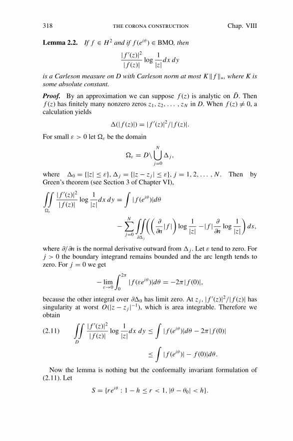
318 the corona construction Chap. VIII
Lemma 2.2. If f ∈ H 2 and if f (eiθ ) ∈ BMO, then
| f ′(z)|2| f (z)| log
1
|z|dx dy
is a Carleson measure on D with Carleson norm at most K‖ f ‖∗, where K issome absolute constant.
Proof. By an approximation we can suppose f (z) is analytic on D. Thenf (z) has finitely many nonzero zeros z1, z2, . . . , zN in D. When f (z) �= 0, acalculation yields
�(| f (z)|) = | f ′(z)|2/| f (z)|.For small ε > 0 let �ε be the domain
�ε = D\N⋃
j=0
� j ,
where �0 = {|z| ≤ ε}, � j = {|z − z j | ≤ ε}, j = 1, 2, . . . , N . Then byGreen’s theorem (see Section 3 of Chapter VI),∫∫
�ε
| f ′(z)|2| f (z)| log
1
|z|dx dy =∫
| f (eiθ )|dθ
−N∑
j=0
∫∫
∂� j
((∂
∂n| f |
)
log1
|z| −| f | ∂
∂nlog
1
|z|)
ds,
where ∂/∂n is the normal derivative outward from � j . Let ε tend to zero. Forj > 0 the boundary integrand remains bounded and the arc length tends tozero. For j = 0 we get
− limε→0
∫ 2π
0
| f (εeiθ )|dθ = −2π | f (0)|,
because the other integral over ∂�0 has limit zero. At z j , | f ′(z)|2/| f (z)| hassingularity at worst O(|z − z j |−1), which is area integrable. Therefore weobtain
∫∫
D
| f ′(z)|2| f (z)| log
1
|z|dx dy ≤∫
| f (eiθ )|dθ − 2π | f (0)|(2.11)
≤∫
| f (eiθ )| − f (0)|dθ.
Now the lemma is nothing but the conformally invariant formulation of(2.11). Let
S = {reiθ : 1 − h ≤ r < 1, |θ − θ0| < h}.
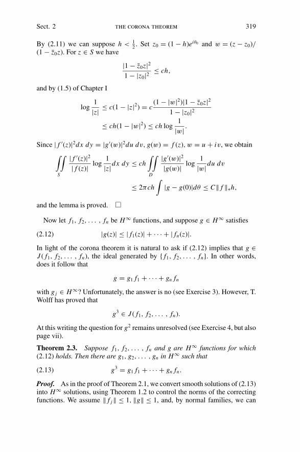
Sect. 2 the corona theorem 319
By (2.11) we can suppose h < 12. Set z0 = (1 − h)eiθ0 and w = (z − z0)/
(1 − z0z). For z ∈ S we have
|1 − z0z|21 − |z0|2 ≤ ch,
and by (1.5) of Chapter I
log1
|z| ≤ c(1 − |z|2) = c(1 − |w|2)|1 − z0z|2
1 − |z0|2
≤ ch(1 − |w|2) ≤ ch log1
|w| .
Since | f ′(z)|2dx dy = |g′(w)|2du dv, g(w) = f (z), w = u + iv, we obtain
∫∫
S
| f ′(z)|2| f (z)| log
1
|z|dx dy ≤ ch∫∫
D
|g′(w)|2|g(w)| log
1
|w|du dv
≤ 2πch∫
|g − g(0)|dθ ≤ C‖ f ‖∗h,
and the lemma is proved.
Now let f1, f2, . . . , fn be H∞ functions, and suppose g ∈ H∞ satisfies
|g(z)| ≤ | f1(z)| + · · · + | fn(z)|.(2.12)
In light of the corona theorem it is natural to ask if (2.12) implies that g ∈J ( f1, f2, . . . , fn), the ideal generated by { f1, f2, . . . , fn}. In other words,does it follow that
g = g1 f1 + · · · + gn fn
with g j ∈ H∞? Unfortunately, the answer is no (see Exercise 3). However, T.Wolff has proved that
g3 ∈ J ( f1, f2, . . . , fn).
At this writing the question for g2 remains unresolved (see Exercise 4, but alsopage vii).
Theorem 2.3. Suppose f1, f2, . . . , fn and g are H∞ functions for which(2.12) holds. Then there are g1, g2, . . . , gn in H∞ such that
g3 = g1 f1 + · · · + gn fn.(2.13)
Proof. As in the proof of Theorem 2.1, we convert smooth solutions of (2.13)into H∞ solutions, using Theorem 1.2 to control the norms of the correctingfunctions. We assume ‖ f j‖ ≤ 1, ‖g‖ ≤ 1, and, by normal families, we can
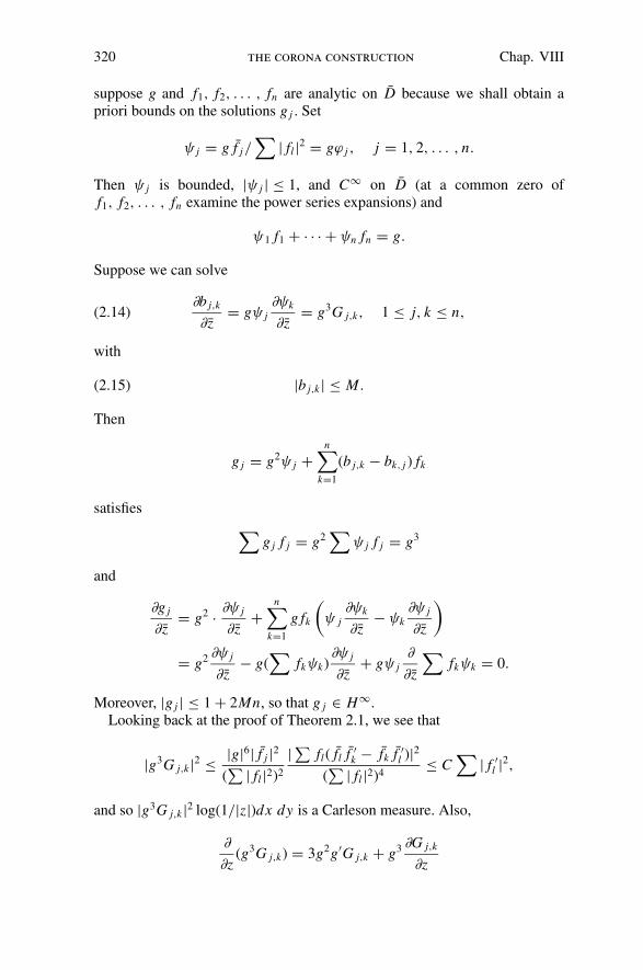
320 the corona construction Chap. VIII
suppose g and f1, f2, . . . , fn are analytic on D because we shall obtain apriori bounds on the solutions g j . Set
ψ j = g f j/∑
| fl |2 = gϕ j , j = 1, 2, . . . , n.
Then ψ j is bounded, |ψ j | ≤ 1, and C∞ on D (at a common zero off1, f2, . . . , fn examine the power series expansions) and
ψ1 f1 + · · · + ψn fn = g.
Suppose we can solve
∂b j,k
∂ z= gψ j
∂ψk
∂ z= g3G j,k, 1 ≤ j, k ≤ n,(2.14)
with
|b j,k | ≤ M.(2.15)
Then
g j = g2ψ j +n∑
k=1
(b j,k − bk, j ) fk
satisfies
∑g j f j = g2
∑ψ j f j = g3
and
∂g j
∂ z= g2 · ∂ψ j
∂ z+
n∑
k=1
g fk
(
ψ j∂ψk
∂ z− ψk
∂ψ j
∂ z
)
= g2 ∂ψ j
∂ z− g(
∑fkψk)
∂ψ j
∂ z+ gψ j
∂
∂ z
∑fkψk = 0.
Moreover, |g j | ≤ 1 + 2Mn, so that g j ∈ H∞.Looking back at the proof of Theorem 2.1, we see that
|g3G j,k |2 ≤ |g|6| f j |2(∑ | fl |2)2
| ∑ fl( fl f ′k − fk f ′
l )|2(∑ | fl |2)4
≤ C∑
| f ′l |2,
and so |g3G j,k |2 log(1/|z|)dx dy is a Carleson measure. Also,
∂
∂z(g3G j,k) = 3g2g′G j,k + g3 ∂G j,k
∂z

Sect. 2 the corona theorem 321
and
|g2g′G j,k | ≤ |g2||g′|| f j |∑ | fl |2| ∑ fl( fl f ′
k − fk f ′l )
(∑ | fl |2)2
|
≤ C(|g′|2 + ∑ | f ′l |2)
(∑ | fl |2)1/2
≤ C|g′|2|g| + C
∑ | f ′l |2
| fl | ,
while∣∣∣∣g
3 ∂G j,k
∂z
∣∣∣∣ ≤ C |g|3 ∑
p,q | f ′p|| f ′
q |(∑ | fl |2)2
≤ Cn∑ | f ′
l |2| fl | ,
by the calculations in the proof of Theorem 2.1. Hence by Lemma 2.2,∂/∂z(g3G j,k) is a Carleson measure with constant depending only on n, andby Theorem 1.2, (2.14) has solutions satisfying (2.15).
Recently Gamelin [1981], and independently A. M. Davie, refined Wolff’sproof still more, even removing the notion of Carleson measure (see Exercise5).
There is a close connection between the corona theorem and the H 1–BMOduality. The theorem was reduced to the question of finding functions b j,k suchthat
∂b j,k
∂ z= ϕ j
∂ϕk
∂ z= G j,k, |z| < 1,(2.16)
and such that
‖b j,k‖∞ = sup|z|=1
|b j,k(z)| ≤ C2(n, δ).
Let
Fj,k(z) = 1
2π i
∫∫
|ζ |<1
G j,k(ζ )1
ζ − zdζ ∧ d ζ(2.17)
be the solution of (2.16) given by the integral formula (1.2). Any solutionof (2.16) has the form b j,k = Fj,k − h j,k, h j,k ∈ H∞, and Corollary 4.6 ofChapter VI gives
c1‖Fj,k − i Fj,k‖∗ ≤ inf{‖b j,k‖∞ : b j,k satisfies (2.16)}≤ c2‖Fj,k − i Fj,k‖∗,
where Fj,k denotes the conjugate function and where c1 and c2 are constants.By (2.17), Fj,k(z) is analytic on |z| > 1, so that Fj,k ∈ H∞, when Fj,k is viewed

322 the corona construction Chap. VIII
as a function only on the circle {|z| = 1}. Also,∫
F j,kdθ = 0 by (2.17). Hence
F j,k = i F j,k and the minimal norm of solutions of (2.16) is comparable to 2‖Fj,k‖∗. When ϕ j is defined by (2.6), the proofs of Theorems 2.1 and 1.2 showby duality that ‖F j,k‖∗ is bounded. We will show later that ϕ j can be chosenso that |G j,k |dx dy is a Carleson measure, and in that case one can directlyverify that ‖F j,k‖∗ ≤ C(n, δ).
The corona problem is equivalent to the problem of finding boundson solutions of equations like (2.16). To prove this, consider the prob-lem of two functions f1 and f2, analytic on a neighborhood of D, thatsatisfy
max(| f1(z)|, | f2(z)|) > δ > 0, |z| ≤ 1,
‖ f1‖ ≤ 1, ‖ f2‖ ≤ 1.
Let ϕ1 and ϕ2 be C∞ solutions of
ϕ1 f1 + ϕ2 f2 = 1
with ‖ϕ‖∞ ≤ C1(2, δ), j = 1, 2. If g1 and g2 are analytic solutions, then sinceg1 f1 + g2 f2 = 1, we have
g1 = ϕ1 + f2
(ϕ2 − g2
f1
)
, g2 = ϕ2 − f1
(g1 − ϕ1
f2
)
.
The function
R = ϕ2 − g2
f1
= g1 − ϕ1
f2
has the bound ‖R‖∞ ≤ C2(2, δ) if and only if ‖g j‖ ≤ C(2, δ), j = 1, 2. Now
∂R
∂ z= 1
f1
∂ϕ2
∂ z= ( f1ϕ1 + f2ϕ2)
f1
∂ϕ2
∂ z
= ϕ1
∂ϕ2
∂ z+ ϕ2
f1
∂
∂ z(1 − f1ϕ1)
= ϕ1
∂ϕ2
∂ z− ϕ2
∂ϕ1
∂ z.
Thus bounded analytic solutions g1, g2 exist if and only if
∂R
∂ z= ϕ
∂ϕ2
∂ z− ϕ2
∂ϕ1
∂ z
can be solved with ‖R‖∞ ≤ C2(2, δ) whenever ϕ1 and ϕ2 are smooth boundedcorona solutions.

Sect. 3 two theorems on minimum modulus 323
3. Two Theorems on Minimum Modulus
Let u(z) be a bounded, complex-valued, harmonic function on the upperhalf plane. Assume ‖u‖∞ ≤ 1. Let Q be a square with base on {y = 0}. For0 < α < 1, set
Eα = {z ∈ Q : |u(z)| ≤ α}and let
E∗α = {x : x + iy ∈ Eα for some y > 0}
be the orthogonal projection of Eα onto {y = 0}. Denote by T (Q) the top halfof Q. Fix β > 0 and suppose there is z0 ∈ T (Q) such that |u(z0)| > β. SeeFigure VIII.1. Since ‖u‖∞ ≤ 1, the Poisson integral representation shows thatfor t ∈ Q∗ = {x : x + iy ∈ Q for some y > 0}, |u(t) − u(z0)| can be largeonly when t is in a set of small measure, provided of course that 1 − β issufficiently small. This in turn implies that |E∗
α|/|Q∗| is small. This reasoningis made precise in the proof of the following theorem.
Theorem 3.1. Let u(z) be harmonic in the upper half plane. Assume ‖u‖∞ ≤1. If 0 < α < 1 and if 0 < ε < 1, then there is β = β(α, ε), 0 < β < 1, suchthat if Q is any square with base on {y = 0}, then
supT (Q)
|u(z0)| ≥ β
implies
|E∗α| ≤ ε(Q).(3.1)
where (Q) = |Q∗| is the edge length of Q.
Figure VIII.1. The situation in Theorem 3.1.

324 the corona construction Chap. VIII
Proof. The appropriate tool for this proof is the vertical maximal function
f +(x) = supy>0
| f (x + iy)|,
where f (z) is a harmonic function on the upper half plane.We may assume Q = {0 ≤ x ≤ 1, 0 < y ≤ 1}. Suppose z0 ∈ T (Q) has
|u(z0)| ≥ β. Then
(∫|u(t) − u(z0)|Pz0
(t)dt
)2
≤∫
|u(t) − u(z0)|2 Pz0(t)dt(3.2)
=∫
|u(t)|2 Pz0(t)dt − |u(z0)|2
≤ 1 − β2.
Let I = [−1, 2] be the triple of the base of Q and let
f (t) = (u(t) − u(z0))χI (t).
Since |Pz0| ≥ c1 on I, we have ‖ f ‖1 ≤ c−1
1 (1 − β2)1/2 by (3.2). Also, for z ∈ Qbut for t �∈ I, Pz(t)/Pz0
(t) ≤ c2, so that when z ∈ Eα ⊂ Q,
| f (z)| =∣∣∣∣
∫f (t)Pz(t)dt
∣∣∣∣
≥∣∣∣∣
∫(u(t) − u(z0))Pz(t)dt
∣∣∣∣ −
∫
�\I|u(t) − u(z0)|Pz(t)dt
≥ (β − α) − c2
∫
�\I|u(t) − u(z0)|Pz0
(t)dt
≥ (β − α) − c2(1 − β2)1/2 = γ,
again by (3.2). Since α is fixed, we can make γ > 0 by taking β sufficientlyclose to one. Then E∗
α ⊂ {t : f +(t) > γ } and the weak-type estimate for f +gives
|E∗α| ≤ Cc−1
1 (1 − β2)1/2/γ.
We conclude that |E∗α| < ε if 1 − β is sufficiently small.
In Theorem 3.1 it is necessary that β be large. For example, if u(t) = 1 −χI (t), with I = [0, 1], then E∗
α = I for every α > 0, while supT (Q) |u(z0)| > 12
when Q is the unit square. Thus we must have β > 12
no matter how small wetake α. However, if the harmonic function is replaced by a bounded analyticfunction f (z), then by exploiting the subharmonicity of log | f (z)|, we can fixany β > 0 and find α = α(β) > 0 so that (3.1) still holds.
Theorem 3.2. Let f (z) be a bounded analytic function on the upper halfplane. Assume ‖ f ‖∞ ≤ 1. For 0 < β < 1 and for 0 < ε < 1, there exists

Sect. 3 two theorems on minimum modulus 325
α = α(β, ε), 0 < α < 1, such that for any square Q with base on {y = 0}supT (Q)
| f (z)| ≥ β
implies
|E∗α| < ε(Q),
where E∗α is the vertical projection onto {y = 0} of
Eα = {z ∈ Q : | f (z)| ≤ α}.Proof. We again suppose that Q is the unit square {0 ≤ x ≤ 1, 0 < y ≤ 1}.Write f = Bg, where B is a Blaschke product with zeros {z j }, and where g(z)has no zeros, ‖g‖∞ ≤ 1. Then
Eα ⊂ Fα ∪ Gα,
where
Fα = {z ∈ Q : |B(z)| <√
α} and Gα = {z ∈ Q : |g(z)| <√
α}.Clearly, E∗
α ⊂ F∗α ∪ G∗
α . We estimate |F∗α | and |G∗
α| separately.To bound |G∗
α| we use Theorem 3.1 on the function u(z) = g(z)p, wherep > 0 will be determined in a moment. Fix α1 > 0 and take β1 = β ′
1(α1, ε/3)so that Theorem 3.1 holds. Let p > 0 satisfy β p = β1. Applying Theorem 3.1to g p, we obtain |G∗
α| < ε/3, provided that α p/2 ≤ α1.The estimate of |F∗
α | is based on the fact that |B(z0)| > β for some z0 =x0 + iy0 ∈ T (Q). By Lemma 1.2 of Chapter VII, this means
∑ 4y0 y j
|z0 − z j |2 ≤ 2 log1
β.(3.3)
Let S = {z j : dist(z j , Q) < 1}. Then |z0 − z j |2/4y0 ≤ 7 when z j ∈ S, andhence
∑
z j ∈S
y j ≤ 14 log 1/β.(3.4)
We excise the discs
� j = {z : |z − z j | < (ε/6)(14 log 1/β)−1 y j }.Taking ε small enough, we can assume � j ∩ Fα = ∅ when z j �∈ S, so thatFα\ ⋃
� j = Fα\ ⋃S � j . By (3.4) we have
∑
z j ∈S
|�∗j | < ε/3,

326 the corona construction Chap. VIII
and so we only have to estimate the size of the projection of Fα\ ⋃S � j . But
when z ∈ Fα\ ⋃� j , Lemma 1.2 of Chapter VII also gives
log1
α≤ log
1
|B(z)|2 ≤ c(ε, β)∑ 4yy j
|z − z j |2 .
In this sum the main contribution comes from the z j ∈ S. Indeed, when z0 ∈T (Q) and z j �∈ S (so that dist(z j , Q) > 1),
supz∈Q
yy j
|z − z j |2 ≤ c1
y0 y j
|z0 − z j |2 ,
and hence by (3.3)
supz∈Q
∑
z j �∈S
4yy j
|z − z j |2 ≤ c1
∑ 4y0 y j
|z0 − z j |2 ≤ 2c1 log1
β.
Taking α ≤ α0(β, ε), we conclude that
2
c(ε, β)log
1
α≤
∑
z j ∈S
4yy j
|z − z j |2(3.5)
holds when z ∈ Fα\ ⋃� j .
Using (3.5) we can estimate |(Fα\ ⋃� j )
∗| in terms of a maximal functionin the same way as before. Consider the positive discrete measure
μ =∑
z j ∈S
4y jδz j .
Then (3.5) gives∫
y
|z − ζ |2 dμ(ζ ) ≥ 2
c(ε, β)log
1
α(3.6)
for z ∈ Fα\ ⋃� j , while on the other hand, (3.4) gives
∫dμ ≤ 56 log
1
β.
Project the mass μ vertically onto {y = 0}. This increases the integral in (3.6).We obtain a positive measure σ on � such that
∫dσ ≤ 56 log 1/β and such
that∫
Pz(t)dσ (t) ≥ 2
πc(ε, β)log
1
α
when z ∈ Fα\ ⋃� j . Consequently,
(Fα\⋃
� j )∗ ⊂ {x : M(dσ ) > (2/πc(ε, β)) log 1/α},

Sect. 4 interpolating blaschke products 327
where M(dσ ) denotes the Hardy–Littlewood maximal function of σ . Theweak-type estimate for M(dσ ) now yields
|(Fα\⋃
� j )∗| ≤ Cπc(ε, β)
2
log 1/β
log 1/α<
ε
3,
provided α is sufficiently small.We conclude that
|E∗α| ≤ |G∗
α| +∑
j
|�∗j | + |(Fα\
⋃� j )
∗| ≤ 3ε
3= ε
if α is small enough.
4. Interpolating Blaschke Products
A Blaschke product is called an interpolating Blaschke product if it hasdistinct zeros and if these zeros form an interpolating sequence. We do notknow if the set of interpolating Blaschke products span a dense subspace ofH∞, as does the set of all Blaschke products (see page vii). However, theinterpolating Blaschke products do separate the points of the upper half planein a very strong way. The precise result is this.
Theorem 4.1. Let u(z) be a bounded harmonic function on the upper halfplane such that
|u(t)| = 1 almost everywhere on �.
Let δ > 0 and let 0 < α < 1. Then there exist β = β(α), 0 < β < 1, and aninterpolating Blaschke product B(z) such that
|B(z)| ≤ δ i f |u(z)| ≤ α(4.1)
and
|u(z)| ≤ β i f B(z) = 0.(4.2)
Moreover if B(z) has zeros {zk}, then
δ(B) = infB(zn )=0
∏
k,k �=n
∣∣∣∣zn − zk
zn − zk
∣∣∣∣(4.3)
≥ δ0(α, β, δ) > 0.
The reader may find Theorem 4.1 acutely specialized. We have put the theoremhere for two reasons. First it will be an essential step in the description of theclosed subalgebras of L∞ containing H∞ given in the next chapter. The secondreason is pedagogical. Its proof using Theorem 3.1 above and generations like
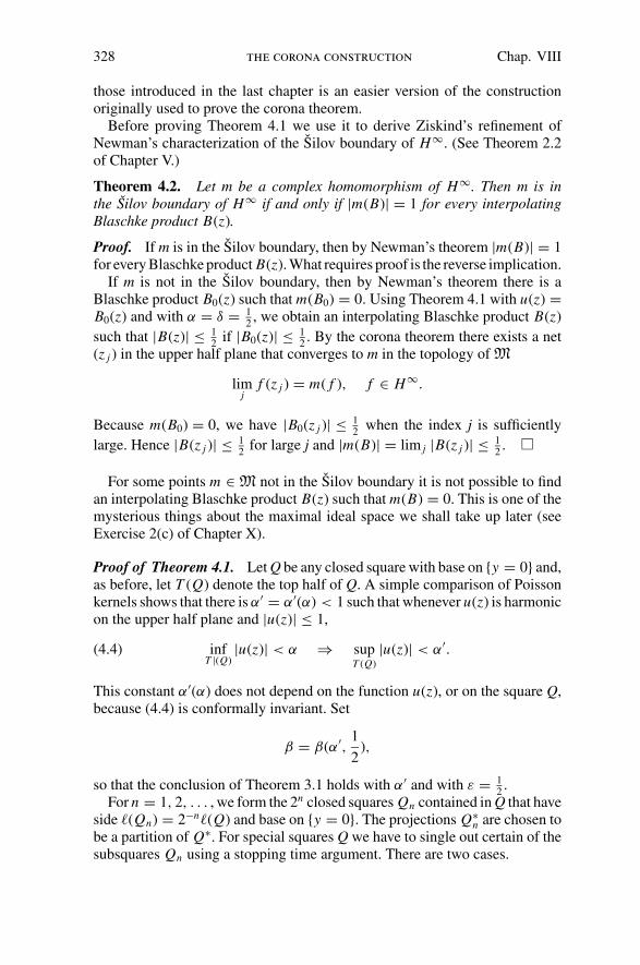
328 the corona construction Chap. VIII
those introduced in the last chapter is an easier version of the constructionoriginally used to prove the corona theorem.
Before proving Theorem 4.1 we use it to derive Ziskind’s refinement ofNewman’s characterization of the Silov boundary of H∞. (See Theorem 2.2of Chapter V.)
Theorem 4.2. Let m be a complex homomorphism of H∞. Then m is inthe Silov boundary of H∞ if and only if |m(B)| = 1 for every interpolatingBlaschke product B(z).
Proof. If m is in the Silov boundary, then by Newman’s theorem |m(B)| = 1for every Blaschke product B(z). What requires proof is the reverse implication.
If m is not in the Silov boundary, then by Newman’s theorem there is aBlaschke product B0(z) such that m(B0) = 0. Using Theorem 4.1 with u(z) =B0(z) and with α = δ = 1
2, we obtain an interpolating Blaschke product B(z)
such that |B(z)| ≤ 12
if |B0(z)| ≤ 12. By the corona theorem there exists a net
(z j ) in the upper half plane that converges to m in the topology of M
limj
f (z j ) = m( f ), f ∈ H∞.
Because m(B0) = 0, we have |B0(z j )| ≤ 12
when the index j is sufficiently
large. Hence |B(z j )| ≤ 12
for large j and |m(B)| = lim j |B(z j )| ≤ 12.
For some points m ∈ M not in the Silov boundary it is not possible to findan interpolating Blaschke product B(z) such that m(B) = 0. This is one of themysterious things about the maximal ideal space we shall take up later (seeExercise 2(c) of Chapter X).
Proof of Theorem 4.1. Let Q be any closed square with base on {y = 0} and,as before, let T (Q) denote the top half of Q. A simple comparison of Poissonkernels shows that there is α′ = α′(α) < 1 such that whenever u(z) is harmonicon the upper half plane and |u(z)| ≤ 1,
infT |(Q)
|u(z)| < α ⇒ supT (Q)
|u(z)| < α′.(4.4)
This constant α′(α) does not depend on the function u(z), or on the square Q,because (4.4) is conformally invariant. Set
β = β(α′,1
2),
so that the conclusion of Theorem 3.1 holds with α′ and with ε = 12.
For n = 1, 2, . . . , we form the 2n closed squares Qn contained in Q that haveside (Qn) = 2−n(Q) and base on {y = 0}. The projections Q∗
n are chosen tobe a partition of Q∗. For special squares Q we have to single out certain of thesubsquares Qn using a stopping time argument. There are two cases.
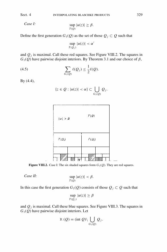
Sect. 4 interpolating blaschke products 329
Case I: supT (Q)
|u(z)| ≥ β.
Define the first generation G1(Q) as the set of those Q j ⊂ Q such that
supT (Q j )
|u(z)| < α′
and Q j is maximal. Call these red squares. See Figure VIII.2. The squares inG1(Q) have pairwise disjoint interiors. By Theorem 3.1 and our choice of β,
∑
G1(Q)
(Q j ) ≤ 1
2(Q).(4.5)
By (4.4),
{z ∈ Q : |u(z)| < α} ⊂⋃
G1(Q)
Q j .
Figure VIII.2. Case I: The six shaded squares form G1(Q). They are red squares.
Case II: supT (Q)
|u(z)| < β.
In this case the first generation G1(Q) consists of those Q j ⊂ Q such that
supT (Q j )
|u(z)| ≥ β
and Q j is maximal. Call these blue squares. See Figure VIII.3. The squares inG1(Q) have pairwise disjoint interiors. Let
R (Q) = (int Q)\⋃
G1(Q)
Q j .

330 the corona construction Chap. VIII
Figure VIII.3. Case II: The shaded squares form G1(Q). They are blue squares. In the regionR (Q) above the blue squares, |u(z)| < β.
Then R (Q) has rectifiable boundary and
length(∂R (Q)) ≤ 6(Q)(4.6)
On R (Q) we have |u(z)| < β. Since u(z) has nontangential limits of absolutevalue 1 almost everywhere, and since β < 1, we also have
|∂R (Q)| ∩ {y = 0}| = 0.(4.7)
Begin with the unit square Q0. Apply Case I or II to Q0, obtaining thefirst generation G1 = {Q1
1, Q12, . . . }. To each Q1
j ∈ G1 we apply Case I or
II and get a new family G1(Q1j ) of generation squares. Define the second
generation to be G2 = ⋃{G1(Q1j ) : Q1
j ∈ G1} = {Q21, Q2
2, . . . }. Repeatingthe process with G2 and continuing inductively, we obtain later generationsG p = {Q p
1 , Q p2 , . . . }. Since α′ < β, we alternate between Case I and Case II
as we move from one generation to the next, and we apply the same case to allsquares in a given generation. In other words, each generation consists entirelyof red squares or blue squares, and the next generation consists only of squaresof the other color. By the construction,
{z ∈ Q0 : |u(z)| < α} ⊂⋃
Case II
R (Q pj ) ⊂ {z ∈ Q0 : |u(z)| < β}.(4.8)
Set
� = Q0 ∩⋃
Case II
∂R (Q pj ).
The important results of this construction are
(a) the arc length measure on � is a Carleson measure, and(b) if B(z) is a bounded harmonic function on {y > 0} and if |B(z)| ≤ δ on
�, then |B(z)| ≤ δ on⋃
Case II R (Q pj ).

Sect. 4 interpolating blaschke products 331
To prove (a) it is enough to check that length (� ∩ Q) ≤ C(Q) when Q =Qn is a square from the decomposition of Q0, because any Q ⊂ Q0 can becovered by two such Qn with (Qn) ≤ 2(Q). So consider a square Q = Qn .There is a smallest index p such that Q contains squares from G p. By (4.5)and (4.6), squares from G p ∪ G p+1 ∪ · · · contribute no more than
∞∑
k=0
6(Q)
2k= 12(Q)
to length(� ∩ Q). The rest of � ∩ Q comes from squares in G p−1 or G p−2,but not both. Their contribution does not exceed 6(Q). Altogether we have
length(� ∩ Q) ≤ 18(Q)
and (a) holds.To prove (b) it is enough to consider one setR (Q) and to show that |B(z)| ≤ δ
on R (Q) if |B(z)| ≤ δ on {y > 0} ∩ ∂R (Q). This follows from (4.7) and aPhragmen–Lindelof argument which we now outline. Because of (4.7), thereare positive harmonic functions Vn(z) on the upper half plane such that
limz→t
Vn(z) = +∞, t ∈ � ∩ ∂R (Q)
and such that
limn→∞ Vn(z) = 0, z ∈ H
(see Exercise 9 of Chapter I). When ζ ∈ ∂R (Q) we then have
limR (Q)�z→ζ
|B(z) + Vn(z)| ≤ δ + limR (Q)�z→ζ
Vn(z).
Indeed, if Im ζ > 0, this inequality follows from the continuity of B(z) + Vn(z),whereas if Im ζ = 0 the inequality is obvious since limz→ζ Vn(z) = +∞. Themaximum principle for subharmonic functions now gives
|B(z) + Vn(z)| ≤ δ + Vn(z), z ∈ R (Q).
Sending n → ∞, we obtain (b).It is now quite easy to find the interpolating Blaschke product B(z). Let
us first construct an interpolating Blaschke product B1(z) that has (4.2) andthat satisfies (4.1) only for points in the unit square Q0. Choose points {z j } in⋃
∂T (Qn), where Qn ranges through all squares in the decomposition of Q0,including Q0 itself, so that
infj
ρ(z j , z) < δ, z ∈⋃
∂T (Qn)(4.9)
and so that
ρ(z j , zk) ≥ η > 0, j �= k.(4.10)
That can be done as follows. Along each ∂T (Qn), mark off equally spacedpoints, 2−N (Qn) units apart, including the corners of T (Qn). Let {z j } be
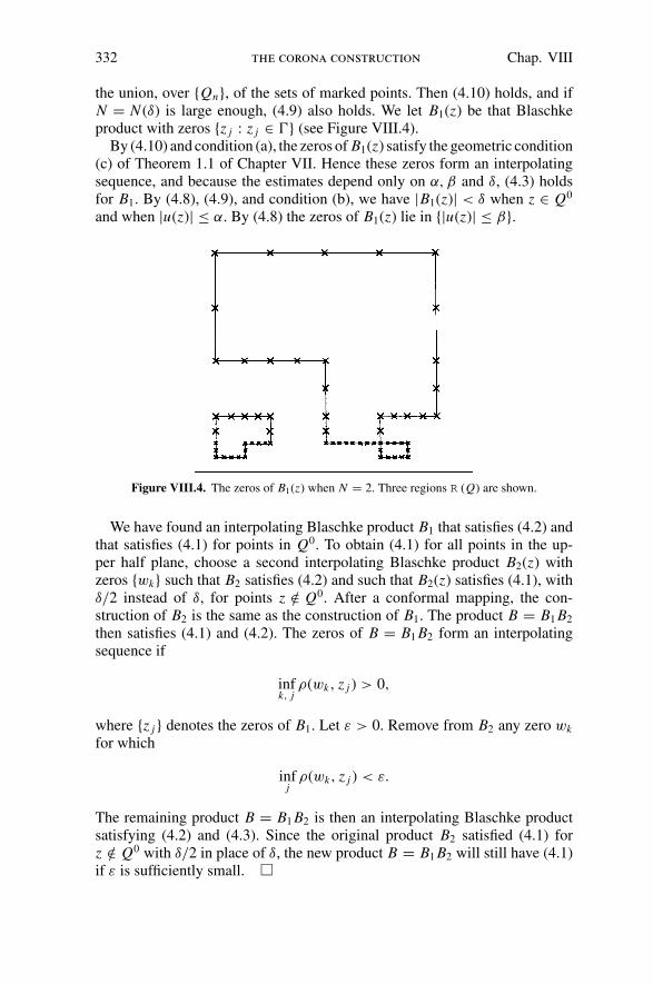
332 the corona construction Chap. VIII
the union, over {Qn}, of the sets of marked points. Then (4.10) holds, and ifN = N (δ) is large enough, (4.9) also holds. We let B1(z) be that Blaschkeproduct with zeros {z j : z j ∈ �} (see Figure VIII.4).
By (4.10) and condition (a), the zeros of B1(z) satisfy the geometric condition(c) of Theorem 1.1 of Chapter VII. Hence these zeros form an interpolatingsequence, and because the estimates depend only on α, β and δ, (4.3) holdsfor B1. By (4.8), (4.9), and condition (b), we have |B1(z)| < δ when z ∈ Q0
and when |u(z)| ≤ α. By (4.8) the zeros of B1(z) lie in {|u(z)| ≤ β}.
Figure VIII.4. The zeros of B1(z) when N = 2. Three regions R (Q) are shown.
We have found an interpolating Blaschke product B1 that satisfies (4.2) andthat satisfies (4.1) for points in Q0. To obtain (4.1) for all points in the up-per half plane, choose a second interpolating Blaschke product B2(z) withzeros {wk} such that B2 satisfies (4.2) and such that B2(z) satisfies (4.1), withδ/2 instead of δ, for points z /∈ Q0. After a conformal mapping, the con-struction of B2 is the same as the construction of B1. The product B = B1 B2
then satisfies (4.1) and (4.2). The zeros of B = B1 B2 form an interpolatingsequence if
infk, j
ρ(wk, z j ) > 0,
where {z j } denotes the zeros of B1. Let ε > 0. Remove from B2 any zero wk
for which
infj
ρ(wk, z j ) < ε.
The remaining product B = B1 B2 is then an interpolating Blaschke productsatisfying (4.2) and (4.3). Since the original product B2 satisfied (4.1) forz /∈ Q0 with δ/2 in place of δ, the new product B = B1 B2 will still have (4.1)if ε is sufficiently small.

Sect. 5 carleson’sconstruction 333
5. Carleson’s Construction
Theorem 5.1. Let δ > 0. If f (z) is analytic on D and if | f (z)| ≤ 1, then thereis ψ(z) ∈ C∞(D) such that
(a) 0 ≤ ψ(z) ≤ 1,(b) ψ(z) = 1 if | f (z)| ≥ δ,(c) ψ(z) = 0 if | f (z)| < ε = ε(δ), and(d)
∫∫s |∂ ψ/∂z|dx dy ≤ A(δ), for every sector
S = {z = reiθ : θ0 < θ < θ0 + , 1 − < r < 1}.The constants ε(δ) > 0 and A(δ) depend only on δ.
Notice that Theorem 2.1 follows easily from this result. Supposef1, f2, . . . , fn ∈ H∞ satisfy ‖ f j‖∞ ≤ 1 and
maxj
| f j (z)| ≥ δ > 0, z ∈ D.
For this δ and for each f j , Theorem 5.1 gives us a function ψ j . Set
ϕ j = ψ j/ f j
∑ψl .
Then |ϕ j (z)| ≤ 1/ε, z ∈ D, and
ϕ1 f1 + · · · + ϕn fn = 1.
To replace the ϕ1 by H∞ functions we boundedly solve the equations
∂b j,k
∂ z= ϕ j
∂ϕk
∂ z, 1 ≤ j, k ≤ n.(5.1)
However, since
∂ϕk
∂ z=
∑ (
ψl∂ψk
∂ z− ψk
∂ψl
∂ z
) /
fk(∑
ψl)2,
condition (d) and Theorem 1.1 ensure that (5.1) has bounded solutions.
Proof of Theorem 5.1. We do the construction in the upper half plane. Infact, we only construct ψ in the unit square Q0 = {0 ≤ x ≤ 1, 0 < y ≤ 1}.Simple conformal mappings and a partition of unity on D can then be used toproduce ψ on the disc.
For each dyadic square Q = { j2−k ≤ x ≤ ( j + 1)2−k, 0 ≤ y ≤ 2−k} con-tained in Q0, we again let T (Q) denote the top half of Q, and we form the 2n
dyadic squares Qn contained in Q, having base on {y = 0}, and having side(Qn) = 2−n−k = 2−n(Q). Thus Q\T (Q) is the union of the two squares Q1.
Let N = N (δ) be a positive integer. For each dyadic square Q of side (Q)with base on {y = 0}, partition T (Q) into 22N−1 dyadic squares Sj of side
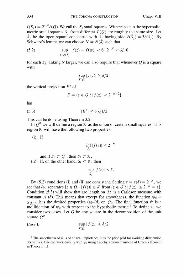
334 the corona construction Chap. VIII
(Sj ) = 2∼N (Q). We call the Sj small squares. With respect to the hyperbolic,metric small squares Sj from different T (Q) are roughly the same size. LetS j be the open square concentric with Sj having side (S j ) = 3(Sj ). BySchwarz’s lemma we can choose N = N (δ) such that
supz,w∈S j
| f (z) − f (w)| < 6 · 2−N < δ/10(5.2)
for each Sj . Taking N larger, we can also require that whenever Q is a squarewith
supT (Q)
| f (z)| ≥ δ/2,
the vertical projection E∗ of
E = {z ∈ Q : | f (z)| < 2−N+2}has
|E∗| ≤ (Q)/2(5.3)
This can be done using Theorem 3.2.In Q0 we will define a region R as the union of certain small squares. This
region R will have the following two properties:
(i) If
infSk
| f (z)| ≤ 2−N
and if Sk ⊂ Q0, then Sk ⊂ R .(ii) If, on the other hand, Sk ⊂ R , then
supSk
| f (z)| < δ.
By (5.2) conditions (i) and (ii) are consistent. Setting ε = ε(δ) = 2−N , wesee that ∂R separates {z ∈ Q : | f (z)| ≥ δ} from {z ∈ Q : | f (z)| ≤ 2−N = ε}.Condition (5.3) will show that arc length on ∂R is a Carleson measure withconstant A1(δ). This means that except for smoothness, the function ψ0 =χQ0\R has the desired properties (a)–(d) on Q0. The final function ψ is amollification of ψ0 with respect to the hyperbolic metric.† To define R weconsider two cases. Let Q be any square in the decomposition of the unitsquare Q0.
Case I: supT (Q)
| f (z)| ≥ δ/2.
† The smoothness of ψ is of no real importance. It is the price paid for avoiding distributionderivatives. One can work directly with ψ0 using Cauchy’s theorem instead of Green’s theoremin Theorem 1.1.

Sect. 5 carleson’sconstruction 335
Consider all Sj ⊂ Q for which
infSj
| f (z)| ≤ 2−N
and such that Sj lies below no other small square with the same property. Welet A(Q) be the family of such Sj . By (5.2) and (5.3), we have
∑
A(Q)
(Sj ) ≤ 1
2(Q),(5.4)
because the projections S∗j of the squares Sj have pairwise disjoint interiors.
For each Sj ∈ A(Q) let Q(1)j be the square with base S∗
j . Each Q(1)j is a dyadic
square with base on {y = 0}, and the interiors of the squares Q(1)j are pairwise
disjoint. Define the first generation
G1(Q) = {Q(1)j : Sj ∈ A(Q)}.
Then by (5.4), we have
∑
G1(Q)
(Q(1)j ) ≤ 1
2(Q).(5.5)
Also let B(Sj ) be the set of Sk such that
S∗k ⊂ S∗
j and (Sj ) ≤ infSk
y ≤ infSj
y.
Thus B(Sj ) consists of Sj and all Sk below Sj except those Sk contained in
Q(1)j . (If we think of Sj as an elevator car on the top floor, then Q(1)
j is theelevator car on the bottom floor, and B(Sj ) is a partition of the elevator shaftwith the bottom floor excluded. See Figure VIII.5.) Notice that
∑
Sk∈B(Sj )
(Sk) ≤ 22N (Sj )(5.6)
because the very small Sk contained in Q(1)j have been excluded. For z ∈ Q we
have | f (z)| > 2−N unless z ∈ ⋃Q(1)
j or z ∈ Sk ∈ B(Sj ), for some Sj ∈ A(Q).Define
R (Q) =⋃
Sj ∈A(Q)
⋃ {
Sk ∈ B(Sj ) : infSk
| f (z)| ≤ 2−N
}
.
If Sk ⊂ Q\ ⋃Q(1)
j , and if infSk | f (z)| ≤ 2−N then Sk ⊂ R (Q). On the otherhand, by (5.2) supSk
| f (z)| < δ if Sk ⊂ R (Q). Thus (i) and (ii) hold for Sk ⊂Q\ ⋃
Q(1)j . By (5.4) and (5.6), ∂R (Q) satisfies
length (∂R (Q)) ≤ 22N+1(Q).(5.7)

336 the corona construction Chap. VIII
Figure VIII.5. A case I square Q when N = 2. The first generation G1(Q) consists of the darklyshaded squares. The squares Sk on which inf | f (z)| < 2−N in R (Q) are lightly shaded.
Case II: supT (Q)
| f (z)| < δ/2.
In this case the first generation G1(Q) consists of those Qn ⊂ Q such that
supQn
| f (z)| ≥ δ/2
and Qn is maximal. The squares Q(1)j in G1(Q) have pairwise disjoint interiors.
Let
R (Q) = Q\⋃
G1(Q)
Q(1)j .
In this case the picture is like Fig. VIII.3. On R (Q) we have | f (z)| ≤ δ/2, andif Sk ⊂ R (Q), then by (5.2), supSk
| f (z)| < δ. Also, we have
(∂R (Q)) ≤ 6(Q) ≤ 22N+1(Q).(5.8)
Starting with the unit square Q0, we apply either Case I or II, and form
the region R (Q0). Then apply either Case I or II to each square Q(1)j in the
first generation G1 = G1(Q0). We obtain new regions R (Q(1)j ) and a second

Sect. 5 carleson’sconstruction 337
generation
G2 =⋃
G1
G1(Q(1)j ),
which consists of all first generation descendants of squares from G1. Continuethis process indefinitely, obtaining succeeding generations G3, G4, . . . . Define
R = R (Q0) ∪∞⋃
p=1
⋃{R (Q(p)
j ) : Q(p)j ∈ G p}.
By the construction, (i) and (ii) hold for Sk ⊂ Q0.
The same case need not apply to all the squares in a given generation G p,but each first generation descendant of a Case II square is a Case I square. Thismeans that we never use Case II two times in succession. By (5.7), (5.8), andespecially (5.5), we see that arc length on ∂R is a Carleson measure. We have
(Q ∩ ∂R ) ≤ 22N+1(Q) + 22N+1∑
{(Q(p)j ) : Q(p)
j ⊂ Q},and, because generation squares are nested, (5.5) gives
∑{(Q(p)
j ) : Q(p)j ⊂ Q} ≤ 2
∞∑
q=1
2−q(Q) = 2(Q).
Consequently we obtain
(Q ∩ ∂R ) ≤ 3 · 22N+1(Q).(5.9)
which shows that arc length on ∂R (Q) is a Carleson measure with constantA = 3 · 22N+1 depending only on δ. Because we want a smooth function ψ(z)we need a slightly different formulation of (5.9). For any Q let
E(Q) = {Sk : Sk ∩ Q ∩ ∂R �= ∅}.
If Sk ∈ E(Q) and if≈Sk is concentric with Sk but nine times as large, then
(Sk) ≤ c(≈Sk ∩Q ∩ ∂R ),
because the only contribution to ∂R within≈Sk comes from squares Sj with
edge length (Sj ) ≥ (Sk)/2. No point lies in more than nine squares Sk , sothat (5.9) yields
∑
E(Q)
(Sk) ≤ c22N+1(Q).(5.10)
338 the corona construction Chap. VIII
For each small square Sj , let ψ j ∈ C∞({y > 0}) satisfy
ψ j = 0 on Sj ,
ψ j ≡ 1 on {y > 0}\S j ,
0 ≤ ψ j ≤ 1, |∇ψ j | ≤ c/(Sj ).
Since no point lies in more than nine squares S j , the function
ψ(z) =∏
Sj ⊂Rψ j (z)
is C∞ on the upper half plane, and
|∇ψ(z)| ≤ c/(Sk), z ∈ Sk .(5.11)
Moreover ∇ψ(z) = 0 except on those squares Sk with Sk ∩ ∂R �= ∅. By (5.10)and (5.11) this means that
∫∫
Q
|∇ψ |dx dy ≤ C2N+1(Q)
for any square Q on {y = 0}. Hence |∇ψ |dx dy is a Carleson measure withconstant A(δ). Clearly 0 ≤ ψ ≤ 1, and (a) holds. By (i) and (ii), conditions (b)and (c) hold for points in Q0.
6. Gradients of Bounded Harmonic Functions
Much of the difficulty with the corona theorem rests in the fact that when f ∈H∞, | f ′(z)|dx dy need not be a Carleson measure. See Chapter VI, Exercise9, for an example. The theorem in this section provides a detour around thatobstruction.
Theorem 6.1. Let u(z) be a bounded harmonic function on the upper halfplane H and let ε > 0. There exists a C∞ function ϕ(z) on H such that
|ϕ(z) − u(z)| < ε(6.1)
and such that |∇ϕ|dx dy is a Carleson measure,
∫∫
Q
|∇ϕ|dx dy ≤ Cε−6‖u‖5∞(Q),(6.2)
whenever Q = {a ≤ x ≤ a + (Q), 0 < y < (Q)}. The constant C in (6.2)is independent of ε and u(z).
Sect. 6 gradients of bounded harmonic functions 339
This theorem is a compromise between something true, that y|∇u|2dx dy isa Carleson measure, and something more desirable but false, that |∇u|dx dyshould be a Carleson measure. Theorem 5.1 is an immediate corollary. Letf ∈ H∞, ‖ f ‖∞ ≤ 1, and let δ > 0. Take h ∈ C∞(�) with h(x) = 1, x >
3δ/4, h(x) = 0, x < δ/2 and with 0 ≤ h(x) ≤ 1. If ϕ is the C∞ function givenby Theorem 6.1 with ε = δ/4, then ψ = h ◦ ϕ has the properties asserted inTheorem 5.1, with ε(δ) = δ/4.
The theorem holds more generally when u(z) is the Poisson integral of aBMO function, and the BMO result, even with ε large, gives yet another proofof the H 1–BMO duality (see Exercise 11). The proof of duality in Chapter VIused the disc analog of the inequality
∫∫
Q
y|∇u|2 dx dy ≤ C‖u‖2∗(Q),(6.3)
which is much more accessible than (6.2). (See Chapter VI, Theorem 3.4, andExercise 5 of that chapter.)
Examples exist for which the function ϕ(z) in Theorem 6.1 cannot be aharmonic function (see Exercise 12).
Theorem 6.1 includes a quantative formulation of Fatou’s theorem. Let u(z)be a bounded harmonic function on {y > 0} and let ε > 0. For x ∈ �, let N ε(x)denote the number of times u(x + iy) oscillates by ε units in the segment0 < y < 1. To be precise, say N ε(x) ≥ n if there are
0 < y0 < y1 < y2 < · · · < yn ≤ 1
such that |u(x + iy j ) − u(x + iy j+1)| ≥ ε. Fatou’s theorem asserts that foreach ε > 0, N ε(x) < ∞ almost everywhere.
Corollary 6.2. If ε > 0, if u(z) is harmonic on {y > 0}, and if ‖u‖∞ ≤ 1,
then∫
IN ε(x)dx ≤ Cε−7
whenever I is an interval of unit length.
Proof. Let ϕ ∈ C∞ satisfy (6.1) and (6.2) with ε/2 in place of ε. If N ε(x) ≥ n,then there are y0 < y1 < y2 < · · · < yn ≤ 1 such that |ϕ(x + iy j ) − ϕ(x +iy j+1)| ≥ ε/3. Hence
∫ 1
0
∣∣∣∣∂ϕ
∂y(x + iy)
∣∣∣∣ dy ≥
n−1∑
j=0
∣∣∣∣∣
∫ y j+1
y j
∂ϕ
∂y(x + iy)dy
∣∣∣∣∣,
≥ nε/3,

340 the corona construction Chap. VIII
and so∫ 1
0|∂ϕ/∂y|dy ≥ N ε(x)ε/3. Then if |I | = 1, (6.2) gives
∫
IN ε(x)dx ≤ 3/ε
∫
I
∫ 1
0
|∇ϕ|dy dx ≤ cε−7,
as desired.
This corollary is suggestive of the theorem on harmonic interpolation se-quences, Theorem 4.2 of Chapter VII, because both results restrict the oscilla-tions of a bounded harmonic function, and one can easily derive the harmonicinterpolation theorem from Corollary 6.2. The connection between Theorem6.1 and harmonic interpolations will be discussed more fully in Chapter X.Corollary 6.2 does not obviously follow from inequality (6.3). However, theanalogous result for averages over dyadic intervals, Lemma 6.4, is an easyconsequence of the martingale version of (6.3). See the remarks after the proofof Lemma 6.4.
The constants ε−7 in Corollary 6.2 and ε−6 in (6.2) are not sharp. Dahlberg[1980] recently obtained ε−1 in (6.2). His local theorem contains Theorem 6.1and a similar result for Poisson integrals of L p functions, p ≥ 2. Dahlberg usesthe Lusin area integral for Lipschitz domains where we shall compare u(z) toa simpler martingale.
Here is the strategy of the proof of Theorem 6.1. We know that y|∇u|2dx dyis a Carleson measure. So at points where u(z) has large oscillation, that is,where y|∇u| ≥ δ(ε), we have |∇u(z)| ≤ δ−1(ε)y|∇u|2. Thus the restriction of|∇u(z)|dx dy to {z : y|∇u(z)| ≥ δ(ε)} is already a Carleson measure, and wecan take ϕ(z) = u(z) on that set. We are left with the set where u(z) has smalloscillation. Temporarily relaxing the requirement that ϕ ∈ C∞, we choose apiecewise constant function ϕ(z) such that |ϕ(z) − u(z)| < ε at almost everypoint where the oscillation is small, and such that ϕ(z) jumps by about ε
units when z crosses the edges of certain dyadic squares. These squares aredetermined by a stopping time argument and they satisfy the nesting condition
∑
Q j ⊂Q
(Q j ) ≤ C(ε)(Q).
As a distribution, |∇ϕ| resembles arc length on the boundaries of the Q j , andhence |∇ϕ| is a Carleson measure. Thus the idea is simply to flatten out thesmall oscillations as much as possible.
It will be convenient to replace Poisson integrals by the averages of u(t)over dyadic intervals.
Lemma 6.3. Let u(z) = Py ∗ u(x) be a bounded harmonic function on theupper half plane and let I be an interval on �. Then for 0 < δ < 1
2,
∣∣∣∣
1
|I |∫
Iu(t)dt − 1
|I |∫
Iu(x + iδ|I |)dx
∣∣∣∣ ≤ cδ log
1
δ‖u‖∞,(6.4)
where the constant c does not depend on u(z), on δ, or on I.

Sect. 6 gradients of bounded harmonic functions 341
Proof. By a change of scale we can take I = [0, 1]. We can also assume‖u‖∞ = 1. Then the left side of (6.4) has supremum ‖F‖1, where
F(t) = χI (t) −∫
IPδ(x − t)dx .
If dist (t, I ) > δ, then
|F(t)| ≤ δ
π
∫
I
dx
(x − t)2= δ
π
(1
dist(t, I )− 1
1 + dist(t, I )
)
.
Hence∫
dist(t,I )>δ
|F(t)|dt ≤ 2δ
π
∫ ∞
δ
(1
s− 1
s + 1
)
= 2δ
πlog
(
1 + 1
δ
)
.
Since ‖F‖∞ ≤ 1 we also have∫
|t |<δ
|F(t)|dt +∫
|1−t |<δ
|F(t)|dt ≤ 4δ.
What remains is the interval J = (δ, 1 − δ). For t ∈ J ,
−F(t) =∫ 0
−∞Pδ(x − t)dx +
∫ ∞
1
Pδ(x − t)dx = G1(t) + G2(t)
and∫
J|G1(t)|dt =
∫
J|G2(t)|dt ≤ δ
π
∫ 1−δ
δ
∫ 0
−∞
dx
(x − t)2dt
<δ
π
∫ 1−δ
δ
dt
t≤ δ
πlog
1
δ.
That establishes (6.4).
Now fix a dyadic interval I and fix a positive integer N. For k = 1, 2, . . . ,partition I into 2Nk closed dyadic intervals Ik of length |Ik | = 2−Nk |I |. Fixε > 0 and let u(t) be an L∞ function defined on I. Define the first generationG1 = G1(I ) to be the set of maximal Ik ⊂ I for which
|uIk − uI | ≥ ε.
The intervals in G1(I ) have pairwise disjoint interiors. For Ik ∈ G1(I ) defineG1(Ik) in the same way and set
G2 = G2(I ) =⋃
{G1(Ik) : Ik ∈ G1}.Later generations G3, G4, . . . are defined inductively, so each Ik ∈ G p+1 iscontained in a unique I j ∈ G p and |uIk − uI j | ≥ ε. Lebesgue’s theorem assertsthat almost every point lies in a finite number of generation intervals. We needa quantitative formulation of that theorem.
342 the corona construction Chap. VIII
Lemma 6.4. For every ε > 0 and for every positive integer N,
∞∑
p=1
∑
I j ∈G p
|I j | ≤ ‖u‖2∞
ε2|I |.
Proof. Set G0 = {I } and set E p = I\ ⋃G p
I j , p = 0, 1, 2, . . . . Define
Yp(t) = u(t)χE p (t) +∑
G p
u I j χI j (t).
Then |Yp − Yp−1| ≥ ε on⋃
G pI j , and hence
∞∑
p=1
∑
G p
|I j | ≤ 1
ε2
∫
I
∞∑
p=1
|Yp − Yp−1|2 dt.
When Ik ∈ G p−1 we have
∫
Ik
Yp dt =∫
Ik∩E p
u(t) dt +∑
I j ⊂IkI j ∈G p
∫
I j
u I j dt
=∫
Ik
u(t) dt = |Ik |uIk ,
and, since Yp−1 = uIk on Ik ,
∫
Ik
YpYp−1 dt = |Ik |u2Ik
=∫
Ik
Y 2p−1 dt.
Similarly, because E p ⊃ E p−1 we have
∫
E p−1
YpYp−1 dt =∫
E p−1
u2(t) dt =∫
E p−1
Y 2p−1 dt.
Consequently,
∫
IYpYp−1 dt =
∫
IY 2
p−1 dt
and∫
I|Yp − Yp−1|2 dt =
∫
IY 2
p dt − 2
∫
IYpYp−1 dt +
∫
IY 2
p−1 dt
=∫
IY 2
p dt −∫
IY 2
p−1 dt.

Sect. 6 gradients of bounded harmonic functions 343
Hence∫
I
∞∑
p=1
|Yp − Yp−1|2 dt = limp→∞
∫
I(|Yp|2 − |Y0|2) dt =
∫
Iu2 dt − u2
I |I |
≤ ‖u‖2∞|I |,
and the lemma is proved.
Lemma 6.4 is really a theorem about martingales. One can view {Yp} asa martingale restricted to a sequence of stopping times. In the proof above,the dominant expression
∑ |Yp − Yp−1|2 is the square of the martingaleS-function. Curiously, the S-function is the analog for martingales of theLittlewood–Paley expression y|∇u|2 dx dy.
Proof of Theorem 6.1. We first find a discontinuous functionϕ2(z) satisfying(6.1) almost everywhere such that the distribution |∇ϕ2| is a Carleson measure.This function will only be constructed in the unit square Q0 = {0 ≤ x ≤ 1, 0 <
y ≤ 1}. A partition of unity can be used to obtain a similar function on theupper half plane. At the end we mollify the latter function into a C∞ functionsatisfying (6.1) and (6.2).
Choose δ = 2−N so that we have
ε
8< cδ log
1
δ<
ε
4
in (6.4). For k = 1, 2, . . . , consider the 2Nk dyadic squares Qk ofthe form Qk = { j2−Nk ≤ x ≤ ( j + 1)2−Nk, 0 < y ≤ 2−Nk}. Set S(Qk) =Qk
∖ ⋃Qk+1 = Qk ∩ {y > 2−N (Qk)}, and let Ik = Q∗
k be the vertical pro-jection of Qk . Write
aQk (u) = 1
|Ik |∫
Ik
u(x + i2−N |Ik |)dx
for the average of u(z) over the bottom edge of S(Qk). By Lemma 6.3 and bythe choice of N,
|aQk (u) − uIk | ≤ (ε/4)‖u‖∞(6.5)
holds for every harmonic function u(z).We say S(Qk) is a blue rectangle if
supS(Qk )
|u(z) − u(w)| ≤ ε/4.(6.6)
A rectangle S(Qk) on which (6.6) fails is called a red rectangle. There are twosteps in the proof. In step I we approximate u(z) on the blue rectangles by apiecewise constant function. In step II we correct the approximation on the redrectangles.
We assume that ‖u‖∞ = 1 and that ε < 1.

344 the corona construction Chap. VIII
Step I: The zero generation G0 consists of the unit square Q0. The firstgeneration G1 = G1(Q0) consists of the maximal Qk ⊂ Q0 for which
|uIk − uI0| ≥ ε/4.(6.7)
When Q j is in the first generation, G1(Q j ) is defined in the same manner.The second generation G2 = G2(Q0) is
⋃{G1(Q j ) : Q j ∈ G1}, and the latergenerations G3, G4, . . . are defined inductively. Except in that we are usingε/4 instead of ε, the generations of squares here correspond naturally to thegenerations of intervals Ik defined before Lemma 6.4. For each generationsquare Q j we form the region
R (Q j ) = Q j∖ ⋃
G1(Q j )
Qk .
Then by (6.7), R (Q j ) is a union of rectangles S(Qn) ⊂ Q j such that |uIn −uI j | < ε/4. By (6.5) this means that
|aQn (u) − aQ j (u)| < 3ε/4,(6.8)
when S(Qn) ⊂ R (Q j ). Each S(Qn) is contained in a unique R (Q j ). Whentwo generation squares Q j and Qk are distinct, their regionsR (Q j ) andR (Qk)have disjoint interiors. Relative to the open upper half plane, ∂R (Q j ) consistsof horizontal and vertical segments. The intersections of these segments fromone ∂R (Q j ) with any square Q have lengths summing to no more than 6(Q).See Figure VIII.6.
Figure VIII.6. The squares Qk if N = 3. The rectangle S(Q0) is blue. On the left a red rectangleS(Q1) has been lightly shaded to indicate that supS(Q1) |u(z) − u(w)| > ε/4. The squares in thefirst generation G1(Q0) are darkly shaded. For a point in the unshaded region, |u(z) − aQ0
(u)| <
ε. The region R (Q0) is the union of the unshaded region and the red rectangle.
For each generation square Q j , including the unit square Q0, define ϕ1(z) =aQ j (u) on the interior R 0(Q j ) of R (Q j ). Thus
ϕ1(z) =∞∑
p=0
∑
Q j∈G p
aQ j (u)χR 0(Q j )(z).
The set⋃
∂R (Q j ), on which ϕ1 has not been defined, has area zero and canbe ignored because for now we are only trying to find ϕ(z) with |ϕ − u| < ε
almost everywhere.

Sect. 6 gradients of bounded harmonic functions 345
Suppose S(Qn) is a blue rectangle. Then by (6.6),
supS(Qn )
|u(z) − aQn (u)| ≤ ε/4 .
There is a unique generation square Q j such that S(Qn) ⊂ R (Q j ), and by(6.8), |aQn (u) − aQ j (u)| < 3ε/4, so that
|ϕ1(z) − u(z)| < ε(6.9)
on S(Qn) ∩ R 0(Q j ). Therefore (6.9) holds almost everywhere on each bluerectangle.
We are interested in |∇ϕ1| only as a distribution on the upper half plane,where
∇ϕ1 =(
∂ϕ1
∂x,∂ϕ1
∂y
)
=∞∑
p=0
∑
Q j ∈G p
aQ j (u)
(∂χR 0(Q j )
∂x,∂χR 0(Q j )
∂y
)
.
As a distribution on {y > 0}, ∂χR 0(Q j )/∂y is the measure −dx along thetop edge of Q j , plus the sum of the measures dx along the other horizontalsegments in {y > 0} ∩ ∂R (Q j ). Similarly, ∂χR 0(Q j )/∂x is a signed sum of themeasures dy on the vertical segments in ∂R (Q j ). Hence |∇χR 0(Q j )| is the arclength measure on � j = {y > 0} ∩ ∂R (Q j ). Since |aQ j (u)| ≤ ‖u‖∞ = 1,
|∇ϕ1| ≤∞∑
p=0
∑
Q j ∈G p
|∇χR (Q j )|
and∫
Q|∇ϕ1| ≤
∑length (Q ∩ � j ),(6.10)
the sum being taken over all generation squares Q j .We claim that
∑length(Q ∩ � j ) ≤ Cε−2(Q)(6.11)
for every square Q resting on y = 0. With (6.10), that proves ∇ϕ1 is a Car-leson measure. In proving (6.11) we can assume that Q is a dyadic squareQ = { j2−n ≤ x ≤ ( j + 1)2−n, 0 < y ≤ 2−n}. Consider first those Q j suchthat Q ∩ � j = Q ∩ ∂R (Q j ) ∩ {y > 0} �= ∅, but such that Q j �⊂ Q. If, in thiscase, (Q j ) ≤ (Q), then Q ∩ � j is a segment along one vertical edge ofQ. These segments are pairwise disjoint, so that these Q j contribute at most2(Q) to the sum (6.11). There can be at most two squares Q j such that(Q j ) > (Q) and such that Q ∩ � j �= ∅. For each of these Q j we have length(Q ∩ � j ) ≤ 6(Q), so these squares contribute no more than 12(Q) in (6.11).
346 the corona construction Chap. VIII
Now consider the generation squares Q j such that Q j ⊂ Q. By Lemma 6.4,
∑
Q j ⊂Q
length(Q ∩ � j ) ≤ 6∑
Q j ⊂Q
(Q j ) ≤ 6(Q) + 16
ε2(Q).
Since ε < 1, we have inequality (6.11) and |∇ϕ1| is a Carleson measure.
Step II: We have found a function ϕ1(z) such that |∇ϕ1| is a Carleson measure,such that ϕ1(z) is constant on the interior of each rectangle S(Qk) and such that|ϕ1 − u| < ε almost everywhere on the blue rectangles S(Qk). Now we approx-imate u(z) on the red rectangles, which are the S(Qk) = {x ∈ Ik, 2−N |Ik | <
y ≤ |Ik |} such that
supS(Qk )
|u(z) − u(w)| > ε/4.
Write
R =⋃
red
{S(Qk)}
for the union of the red rectangles.Let S(Qk) be a red rectangle and take z1, z2 ∈ S(Qk) such that |u(z1) −
u(z2)| > ε/4. At some point z0 on the segment joining z1 to z2 we have
|z1 − z2||∇u(z0)| > ε/4.
Since |z1 − z2| <√
2(Qk) < 2N+1 Im z0 = 2N+1 y0, this gives
2N+3 y0|∇u(z0)| > ε,
so that by the subharmonicity of |∇u|2,∫∫
|z−z0|<y0/2
y|∇u|2dx dy ≥ 1
2y0
∫∫
|z−z0|<y0/2
|∇u|2dx dy
≥ cε22−2N y0.
Letting S(Qk) = ⋃z0∈S(Qk ){z : |z − z0| < Im z0/2}, we obtain
∫∫
S(Qk )
y|∇u|2dx dy ≥ cε22−3N (Qk) .(6.12)
No point lies in more than four regions S(Qk). Because y|∇u|2 is a Carlesonmeasure, (6.12) then yields
∑{(Qk): Qk ⊂ Q, S(Qk) red} ≤ cε−223N (Q)(6.13)
for every square Q. In particular, the arc length ∂R is a Carleson measure withconstant cε−223N .
Sect. 6 gradients of bounded harmonic functions 347
On the other hand, the inequality y|∇u| ≤ c yields∫∫
S(Qk )
|∇u|dx dy ≤ c∫∫
S(Qk )
dx dy
y= cN(Qk)(6.14)
for any rectangle S(Qk). When S(Qk) is red, (6.12) and (6.14) give∫∫
S(Qk )
|∇u|dx dy ≤ cNε−223N∫∫
S(Qk )
y|∇u|2dx dy,(6.15)
so that |∇u(z)|χR (z)dx dy is a Carleson measure with constant cNε−223N .Now define
ϕ2(z) ={
ϕ1(z), z �∈ R ,
u(z), z ∈ R .
Then |ϕ2(z) − u(z)| < ε almost everywhere on H . As a distribution
∇ϕ2 = χQ0\R ∇ϕ1 + χR ∇u + J,
where the remainder term J accounts for the jumps in ϕ2(z) as z crosses ∂R .Since |ϕ2| < 1 + ε, J is a measure and |J | is dominated by 1 + ε times arclength on ∂R. Thus by (6.13), |J | is a Carleson measure with constant C23N ε−2.By (6.15), χR |∇u|dx dy is also a Carleson measure, with constant C N23N ε−2.In the discussion of step I we showed |∇ϕ1| is a Carleson measure with constantCε−2. The integer N was chosen so that N2−N ∼ ε and the worst constant inthe three estimates comes from χR |∇u|dx dy. We obtain
∫
Q|∇ϕ2|dx dy ≤ Cε−6(Q)(6.16)
for every square Q.We have built a function ϕ2 on the unit square Q0 such that |∇ϕ2| satisfies
(6.16) and such that |ϕ2 − u| < ε almost everywhere on Q0. Using a partitionof unity, it is now easy to get a function ϕ3 on H such that |ϕ3 − u| < ε almosteverywhere onH and such that |∇ϕ3| satisfies (6.16). A C∞ function satisfying(6.1) and (6.2) can now be obtained by mollifying ϕ3. Let h(z) ∈ C∞(�2) besuch that h(z) ≥ 0,
∫h(z)dx dy = 1 and h(z) = 0 if |z| ≥ 1. Assume also
that h(z) is radial, h(z) = h(|z|). For δ > 0, set hδ(z) = (1/δ2)h(z/δ). Thenϕ3 ∗ hδ is C∞. If δ < Im z, then |ϕ3 ∗ hδ(z) − u(z)| < ε, because u ∗ hδ(z) =u(z) since u is harmonic and hδ is radial. To keep δ < Im z, partition {y > 0}into strips Tn = {2−n ≤ y ≤ 2−n+1} and set Tn = Tn ∪ Tn+1 ∪ Tn−1. Choosegn = gn(y) ∈ C∞ such that gn is supported on Tn , such that 0 ≤ gn ≤ 1 and|∇gn| = |∂gn/∂y| ≤ c2n , and such that
∑∞−∞ gn = 1 on {y > 0}.
ϕ(z) =∞∑
−∞gn(y)(ϕ3 ∗ h2−n−2)(z)

348 the corona construction Chap. VIII
is C∞ and |ϕ(z) − u(z)| < ε. For z ∈ Tn, ϕ3 ∗ h2−n−2(z) = ϕ3(z) if
dist(z, ∂R ∪⋃
� j ) ≥ 2−n−2
because thenϕ3 is harmonic on |w − z| < 2−n−2. Thus we only have to estimate|∇ϕ|dx dy on
V =∞⋃
−∞Tn ∩ {
z : dist(z, ∂R ∪⋃
� j ) < 2−n−2}.
Fix a dyadic square Q = { j2−p ≤ x ≤ ( j + 1)2−p, 0 < y ≤ 2−p}, p an inte-ger. Then because
∇ϕ(z) =∞∑
−∞(ϕ3 ∗ h2−n−2 (z))∇gn(z) +
∞∑
−∞gn(z)(∇ϕ3 ∗ h2−n−2 )(z),
we have
∫∫
Q∩V
|∇ϕ(z)|dx dy ≤ c∞∑
n=p−1
2n|Q ∩ V ∩ Tn|
+∞∑
n=p−1
∫
Q∩Tn
|∇ϕ3| ∗ h2−n−2 (z) dx dy.
Since |Q ∩ V ∩ Tn| ≤ c2−n length (Q ∩ Tn ∩ (∂R ∪ ⋃� j )), the first sum is
bounded by cε−6(Q). The second sum does not exceed
∞∑
n=p−1
∫
Wn
|∇ϕ3|,
where Wn = {z : dist(z, Q ∩ Tn) ≤ 2−n−2}. These sets Wn are locally finite,no point lies in more than five Wn . The union
⋃n≥p−1 Wn is contained in a
square 16 times as large as Q. Hence
∞∑
n=p−1
∫
Wn
|∇ϕ| ≤ Cε−62−p.
Since (Q) = 2−p, we see that ϕ(z) satisfies (6.2). That completes the proofof the theorem.

Sect. 7 a constructive solution of ∂b/∂z = μ 349
7. A Constructive Solution of ∂b/∂z = μ
To prove the corona theorem we used a duality argument to get the crucialestimate
‖b‖∞ ≤ C supS
1
(S)
∫
S|G|dx dy(7.1)
for some solution of the equation
∂b/∂ z = G(z), |z| < 1.
Recently Peter Jones found a direct way to obtain (7.1). His method simulta-neously yields a constructive proof of the basic decomposition
ϕ = u + Hv, u, v ∈ L∞,(7.2)
of a BMO function. The construction is quite explicit and it should have furtherapplications.
Let μ be a Carleson measure on the upper half plane. Assume μ is positiveand normalized, so that
N (μ) = supQ
μ(Q)/(Q) ≤ 1.
Jones solved
∂b/∂ z = μ, Im z > 0,(7.3)
with |b(t)| ≤ C almost everywhere on �, by exploiting the relation betweenCarleson measures and interpolating sequences. First consider a very specialcase.
Case I: μ = ∑α j y jδz j , where {z j } is a finite sequence of points such that
∏
j ; j �=k
∣∣∣∣zk − z j
zk − z j
∣∣∣∣ ≥ δ > 0(7.4)
with δ a fixed constant, and where 0 ≤ α j ≤ 1. Let B1(z) be the Blaschkeproduct with zeros {z j }. By Green’s theorem the distribution (∂/∂ z)(1/B1(z))equals
∑
j
π
B ′1(z j )
δz j =∑
j
β j y jδz j ,
where 1 ≤ |β j | ≤ 1/δ. By Earl’s proof of the interpolation theorem (Theorem5.1 of Chapter VII) there is a second Blaschke product B2(z) with zeros ζ j
satisfying
ρ(z j , ζ j ) ≤ δ/3
350 the corona construction Chap. VIII
such that
K δ−3 B2(z j ) = α j/β j ,
where K is an absolute constant. The rational function
b(z) = K δ−3(B2(z)/B1(z))
solves (7.3) and |b(t)| ≤ K δ−3 on �.
Case II: Again μ is a positive discrete measure with finite support, μ =∑α j y jδz j , but N (μ) ≤ 1 and the coefficients α j are rational, α j = k j/N . The
main difference between Cases II and I is that here the constant δ in (7.4) maybe very small. Since N (μ) ≤ 1, we have 1 ≤ k j ≤ N . Relabeling the pointsso that z j occurs with multiplicity k j , we have
μ = 1
N
∑y jδz j .
The top half of any square Q resting on {y = 0} contains at most 2N pointsz j , counting multiplicities, because N (μ) ≤ 1. We are going to partition {z j }into 4N interpolating sequences having uniformly bounded constants. Write
Sn = {z j : 2−n−1 < y j ≤ 2−n}and order the z j ∈ Sn according to increasing real parts Sn = {xk,n + iyk,n}with
xk−1,n ≤ xk,n ≤ xk+1,n.
Split {z j } into 2N subsequences Y1, Y2, . . . , Y2N , evenly distributing the pointsin each Sn . That is, put z j = xk,n + iyk,n in Yp if and only if k ≡ p mod(2N ).Fix a dyadic square Q and let Mn(Q) be the number of points z j in Sn ∩ Q.The subsequences have been chosen so that each set Yp ∩ Sn ∩ Q contains atmost
1 + Mn(Q)/2N
points z j . Consequently
∑
Yp∩Q
y j ≤∑
2−n≤(Q)
(
1 + Mn(Q)
2N
)
2−n
≤∑
2−n≤(Q)
2−n + 1
2N
∑
z j ∈Q
2y j
≤ 2(Q) + μ(Q) ≤ 3(Q).
Also, the points in Yp ∩ ⋃n even Sn are very well separated. Two points from
one of these subsequences satisfy
|z j − zk | ≥ y j/2.

Sect. 7 a constructive solution of ∂b/∂z = μ 351
Thus each Yp is the union of two interpolating sequences having large constantsδ in (7.4). By the very special case treated above, we have a rational functionbp(z) such that
∂bp
∂ z=
∑
Yp
y jδz j
and |bp(t)| ≤ C ′, t ∈ �. Then
b(z) = 1
N
2N∑
p=1
bp(z)
is a solution of (7.3) and
|b(t)| ≤ C, t ∈ �,
with C independent of N.
Case III: Now let μ be any positive measure on H such that N (μ) ≤ 1.There is a sequence {μn} of measures of the type treated in Case II such that
∫ϕ dμn →
∫ϕ dμ, ϕ ∈ C∞
0 (H ),
and such that∫
| f |dμn →∫
| f |dμ, f ∈ H 1.
(First restrict μ to a compact subset ofH . Then partitionH into hyperbolicallysmall squares and concentrate the mass of each square at its center.) Let bn(z) bethe solution of ∂bn/∂ z = μn obtained in Case II. Then {bn(t)} converges weak-star to b(t) ∈ L∞ and ‖b‖∞ ≤ C . Moreover, {bn(z)} converges to a distributionsolution of (7.3) on the upper half plane. For applications this distribution mustbe reconciled with its boundary function b(t), but that is not a serious difficulty.To avoid unimportant technicalities, let us move to the unit disc. Then bn(z) isa rational function with no poles on ∂D, and by residues,
1
2π i
∫
|z|=1
f (z)bn(z)dz =∫
Df (z)dμn(z), f ∈ H 1.
Consequently we have
1
2π i
∫
|z|=1
f (z)b(z)dz =∫
Df (z)dμ(z), f ∈ H 1.(7.5)
Now (7.5) is an interpretation of ∂b/∂ z = μ sufficient for our applications.�
In the corona problem we had dμ = (1/π )G dx dy, with G ∈ C∞(D),and by (1.2) we had a function F ∈ C(D) ∩ C∞(D), with ∂F/∂ z = G(z).
352 the corona construction Chap. VIII
Then by Green’s theorem
1
2π i
∫
|z|=1
f (z)F(z)dz = 1
π
∫∫
D
f (z)G(z)dx dy.
By (7.5) this means h(eiθ ) = F(eiθ ) − b(eiθ ) ∈ H∞, and so
b(z) = F(z) − h(z)
is a smooth solution bounded on the disc that satisfies |b(eiθ )| ≤ C almosteverywhere. If we put such functions b(z) into (2.7) we obtain a proof of thecorona theorem without recourse to duality.
Jones’s approach is even more transparent in the notation of distributionderivatives. Then our differential equation is
∂b/∂ z = μ,
where μ can be taken absolutely continuous to arc length on a contour � of thetype constructed in Section 4 or 5. On � arc length is a Carleson measure andthe density defining μ is bounded above and below. In this case the interpolatingBlaschke products are easy to visualize; they resemble the Blaschke productconstructed in Section 4. The solution b(z) can be recognized as an average ofinterpolating Blaschke products. (See the example at the end of this section.)
To prove the decomposition (7.2) let ϕ be a real function in BMO(T ), ‖ϕ‖∗ ≤1. By Exercise 13 of Chapter VI, there exist ψ ∈ L∞, ‖ψ‖∞ ≤ A, and F(z) ∈C∞(D) and g ∈ L1 such that
|F(reiθ )| ≤ g(eiθ ),
such that
ϕ(θ ) = ψ(θ ) + limr→1
F(reiθ ) = ψ(θ ) + F(θ ),
and such that |∇F |dx dy is a Carleson measure with N (|∇F |dx dy) ≤ A. Letb(z) be the solution of
∂b
∂ z= 1
π
∂F
∂ zdx dy
given by Jones’s procedure. Then |b(θ )| ≤ C A and
ϕ = ψ + b + (F − b)
almost everywhere on T. Arguing formally for a moment, we have (F − b)∼ =−i(F − b), because F − b is analytic, and so
ϕ = ψ + b + i F − i b.
Taking real parts, we obtain
ϕ = (ψ + Re b) + (Im b)∼,

Sect. 7 a constructive solution of ∂b/∂z = μ 353
which is (7.2). To make this reasoning precise, notice that by (7.5)
1
2π i
∫znb(z)dz = 1
π
∫∫
D
zn ∂F
∂ zdx dy.
On the other hand, since |F(reiθ )| ≤ g(θ ) ∈ L1, dominated convergence gives
1
2π i
∫zn F(z)dz = 1
π
∫∫
D
zn ∂F
∂ zdx dy.
Consequently F(eiθ ) − b(eiθ ) ∈ H 1, so that we really do have
(F − b)∼ = −i(F − b).
An attractive aspect of this approach to (7.2) is that the Varopoulos construc-tion of F(z) is very explicit. The method in this section also gives a constructiveway of finding g ∈ H∞ such that
‖ f − g‖∞ ≤ C dist ( f, H∞)
when f ∈ L∞.For an example, write x ∈ [0, 1] in base 5, x = ∑
αk5−k , and let ϕ(x) =∑χEk (x), Ek = {x : αk = 1 or αk = 3}. Then ϕ ∈ BMO (see Figure VIII.7).
Figure VIII.7. The function ϕ(x).
If F(x, y) is constructed with pentadic squares instead of dyadic squares, then
F(x, y) =∑
k
χEk (x)χ(0,5−k )(y).
Then ϕ(x) = limy→0 F(x, y) and |∇F | is bounded by arc length on the curvesin H pictured in Figure VIII.8. Cut these curves into segments of bounded hy-perbolic length, uniformly parametrized by t, 0 < t < 1. For each t, let B1(t, z)be the Blaschke product with one zero on each segment at position t. The zerosof B1(t, z), form an interpolating sequence, with constant δ independent of t.They are marked by crosses in Figure VIII.8, for t = 0.8, say. The boundedsolution of ∂b/∂ z = ∂F/∂ z is
b(x) = c∫ 1
0
B2(t, x)
B1(t, x)dt,
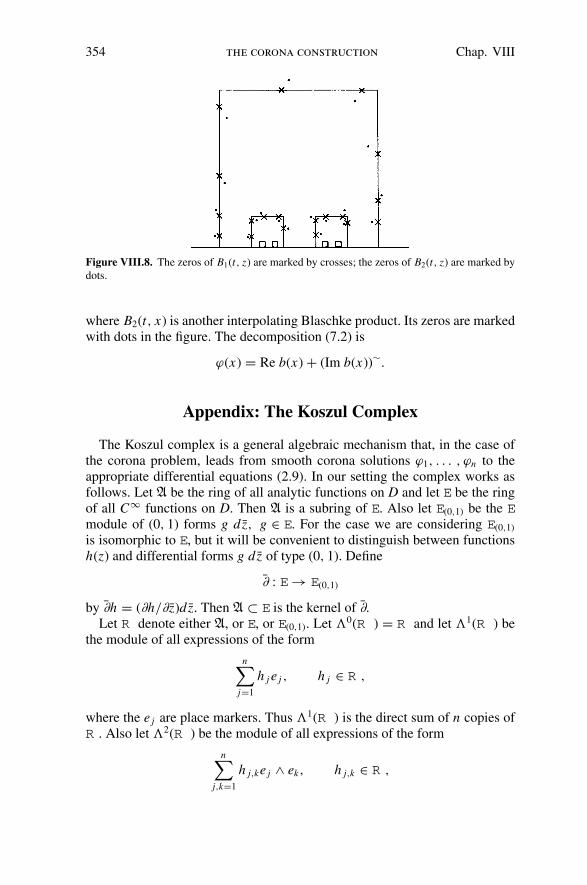
354 the corona construction Chap. VIII
Figure VIII.8. The zeros of B1(t, z) are marked by crosses; the zeros of B2(t, z) are marked bydots.
where B2(t, x) is another interpolating Blaschke product. Its zeros are markedwith dots in the figure. The decomposition (7.2) is
ϕ(x) = Re b(x) + (Im b(x))∼.
Appendix: The Koszul Complex
The Koszul complex is a general algebraic mechanism that, in the case ofthe corona problem, leads from smooth corona solutions ϕ1, . . . , ϕn to theappropriate differential equations (2.9). In our setting the complex works asfollows. Let A be the ring of all analytic functions on D and let E be the ringof all C∞ functions on D. Then A is a subring of E. Also let E(0,1) be the Emodule of (0, 1) forms g dz, g ∈ E. For the case we are considering E(0,1)
is isomorphic to E, but it will be convenient to distinguish between functionsh(z) and differential forms g dz of type (0, 1). Define
∂ : E → E(0,1)
by ∂h = (∂h/∂z)dz. Then A ⊂ E is the kernel of ∂.Let R denote either A, or E, or E(0,1). Let �0(R ) = R and let �1(R ) be
the module of all expressions of the form
n∑
j=1
h j e j , h j ∈ R ,
where the e j are place markers. Thus �1(R ) is the direct sum of n copies ofR . Also let �2(R ) be the module of all expressions of the form
n∑
j,k=1
h j,ke j ∧ ek, h j,k ∈ R ,
Sect. 7 appendix: the koszul complex 355
where we require that
e j ∧ ek = −ek ∧ e j ,(A.1)
a familiar condition in alternating linear algebra. Thus �2(R ) has dimensionn(n − 1)/2 over R . We define
∂ : �p(E ) → �p(E(0,1)), p = 0, 1, 2,
by differentiating the coefficients of the place markers e j or e j ∧ ek . That is,
∂(∑
h j e j
)=
∑(∂h j )e j and ∂
(∑h j,ke j ∧ ek
)=
∑∂h j,ke j ∧ ek .
Then �p(A) ⊂ �p(E ) is the kernel of ∂. Using (1.2), and a partition of unity ifour functions are not bounded, we see that for each p = 0, 1, 2 the ∂ mappingis surjective. This means the sequence
0 → �p(A) → �p(E )∂→ �p(E(0,1)) → 0
is exact; at each step the kernel of the outgoing map is the range of the incomingmap. Let τ ∈ �p(E ), p = 0, 1 and letω ∈ �q (R ), q = 0, 1, whereR is eitherof the Emodules E or E(0,1). The wedge product τ ∧ ω ∈ �p+q (R ) is definedby setting
f ∧ g = f g,
f ∧ ge j = f e j ∧ g = f ge j ,
f e j ∧ gek = f ge j ∧ ek,
and by requiring that τ ∧ ω be E-bilinear; that is, τ ∧ ω is to be E-linear ineach variable.
Now let f1, f2, . . . , fn be corona data. For p = 1, 2, define
J : �p(R ) → �p−1(R )
by
J (he j1 ∧ e j2 ∧ · · · ∧ e jp ) =p∑
k=1
(−1)k+1 f jk he j1 ∧ · · · ∧ e jk ∧ · · · ∧ e jp ,
where the circumflex over a marker e jk indicates that e jk is deleted. The mappingJ is then defined on the full module �p(R ) by requiring that J be R -linear.The factors (−1)k+1 make the definition of J consistent with the alternatingcondition (A.1). In particular
J
(n∑
j=1
g j e j
)
=n∑
j=1
f j g j .
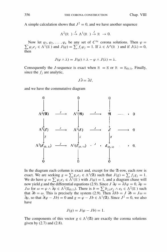
356 the corona construction Chap. VIII
A simple calculation shows that J 2 = 0, and we have another sequence
�2(R )J→ �1(R )
J→ R → 0.
Now let ϕ1, ϕ2, . . . , ϕn be any set of C∞ corona solutions. Then ϕ =∑ϕ j e j ∈ �1(E ) and J (ϕ) = ∑
f jϕ j = 1. If λ ∈ �p(R ) and if J (λ) = 0,then
J (ϕ ∧ λ) = J (ϕ) ∧ λ − ϕ ∧ J (λ) = λ.
Consequently the J-sequence is exact when R = E or R = E(0,1). Finally,since the f j are analytic,
J ∂ = ∂J,
and we have the commutative diagram
In the diagram each column is exact and, except for the A-row, each row isexact. We are seeking g = ∑
g j e j ∈ �1(A) such that J (g) = ∑f j g j = 1.
We do have ϕ = ∑ϕ j e j ∈ �1(E ) with J (ϕ) = 1, and a diagram chase will
now yield g and the differential equations (2.9). Since J ∂ϕ = ∂Jϕ = 0, ∂ϕ =Jω for ω = ϕ ∧ ∂ϕ ∈ �2(E(0,1)). There is b = ∑
b j,ke j ∧ ek ∈ �2(E ) suchthat ∂b = ω. This is precisely the system (2.9). Then ∂Jb = J ∂b = Jω =∂ϕ, so that ∂(ϕ − Jb) = 0 and g = ϕ − Jb ∈ �1(A). Since J 2 = 0, we alsohave
J (g) = J (ϕ − Jb) = 1.
The components of this vector g ∈ �1(A) are exactly the corona solutionsgiven by (2.7) and (2.8).

notes 357
For the corona problem on a domain in �n, n > 1, the Koszul complexhas longer rows and columns, but it does reduce the problem to a system ofdifferential equations.
Notes
Theorem 1.1 is in Carleson [1962a], while Theorem 1.2 is a recent ideaof Wolff’s [1980]. Theorem 2.1 is due to Carleson [1962a], but the line ofreasoning in Section 2 comes from Wolff [1980].
The connection between the corona theorem and differential equations andthe Koszul complex was noticed by Hormander [1967a] (see also Carleson[1970]), but the basic difficulties have remained the same as they were inCarleson [1962a].
Theorem 3.2 is from Carleson’s exposition [1970]. The theorems in Section3 can also be derived from a theorem on harmonic measures known as Hall’slemma. Let E be a compact subset of the upper half plane such that � = H \Eis connected, and let ω(z), z ∈ �, be the harmonic measure of E. Hall’s lemmais the estimate
ω(z) ≥ 2
3
1
π
∫
E
y
(|x | + t)2 + y2dt,
where E = {|z| : z ∈ E} is the angular projection of E onto the positive realaxis and where the Poisson kernel represents the image−|x | + iy of z = x + iyunder a folding. For the proof see Duren [1970] or Hall [1937]. By means ofelementary conformal mappings this inequality gives bounds on the lengthsof vertical projections. Hall’s lemma has certain advantages because it givessimple relations between the numbers α and β of Theorems 3.1 and 3.2 (seeExercise 7). On the other hand, the proof in the text illustrates the power ofmaximal functions. Incidentally, the best constant to replace 2
3in Hall’s lemma
is not known (Hayman [1974]).Theorem 4.1 is due to Marshall [1976b]. Ziskind [1976] had obtained a
slightly weaker result in the course of proving Theorem 2.2. The construction ofthe contour � originates in Carleson’s [1962a] fundamental paper. If � is takento be a level set, |u(z)| = v will not work and it is necessary to approximatethe level sets by shorter curves (see Exercise 8 below).
Theorem 6.1 is motivated by the work of Varopoulos [1977a, b]. The phi-losophy that harmonic functions mimic very simple martingales is delightfullyexpressed in Fefferman’s lecture [1974]. Dahlberg [1980] has improved uponTheorem 6.1 substantially.
The results in Section 7 come from Jones [1980b]. The extension F(z), soeffective in the proof of (7.2), is due to Varopoulos [1977a]. Finding a construc-tive proof of the euclidean space analog of (7.2) is an important open problem inreal analysis. As is often the case with higher-dimensional generalizations, the

358 the corona construction Chap. VIII
real question here is how to eliminate Blaschke products from the construction.See page vii.
Exercises and Further Results
1. Let G(z) be continuous on the open unit disc. Suppose that on |z| <
1 − 1/n there is bn(z) ∈ C1 such that
∂bn/∂ z = G
and |bn| ≤ K , with K independent of n. Then by a normal families argumentthere is b(z) of class C1 such that ∂b/∂z = G on |z| < 1.
2. (a) If G is a bounded function of compact support in the plane and if
F(z) = 1
2π i
∫∫G(ζ )
ζ − zdζ ∧ d ζ ,
then F is bounded and continuous and ∂F/∂ z = G in the distribution sense.(b) Let f (z) be a bounded analytic function on an open set W in the complex
plane and let λ ∈ ∂W . Declare f = 0 on �\W . Let χ (z) ∈ C∞0 have support
{|z − λ| < ε}. Suppose 0 ≤ χ ≤ 1, χ = 1 on {|z − λ| < ε/2}, and |∂χ/∂ z| ≤c/ε. Then
F(z) = −1
2π i
∫∫f (ζ ) − f (z)
ζ − z
∂χ
∂ζdζ ∧ d ζ ,
has the following properties:
(i) ∂F/∂z = χ∂ f/∂ z, as distributions,(ii) F(z) is analytic on W ∪ {|z − λ| > ε},
(iii) |F(z)| ≤ C sup {| f (ζ )| : |ζ − λ| < ε, and(iv) F(z) − f (z) is continuous on {|z − λ| < ε/2}.
(c) Let � be an open set in the plane and let f1, f2, . . ., fn ∈ H∞(�), thebounded analytic functions on �. If there is a finite open cover {Uk}N
k=1 of
� and if there are g(k)j ∈ H∞(� ∩ Uk) such that
∑j f j g
(k)j = 1 on � ∩ Uk ,
then there are g1, g2, . . . , gn ∈ H∞(�) such that∑
f j g j = 1. Let χk ∈C∞
0 (Uk),∑
χk = 1 on �. Perturb the C∞ solutions ϕ j = ∑k χk g(k)
j to getanalytic solutions g j . Use part (a) to solve the Cauchy–Riemann equations(2.9).
(d) From the assumption that the disc is dense in M it follows that there ex-ists a constant C(n, δ) such that every corona problem (2.1), (2.2) in the disc hassolutions satisfying ‖g j‖ ≤ C(n, δ). For the proof it is enough to establish thecorona theorem for the open set W = ⋃∞
k=1{−1 < x < 1, 2−k−1 < y < 2−k},which is conformally equivalent to an infinite disjoint union of discs. So

exercises and further results 359
let f1, f2, . . . , fn ∈ H∞(W ) satisfy ‖ f ‖∞ ≤ 1, max j | f j (z)| ≥ δ, z ∈ W .By the localization theorem in part (c) we only have to find solutionson W ∩ {|z − λ| < η}, for some η > 0, for −1 ≤ λ ≤ 1. By part (b) thereis a bounded simply connected domain �λ containing W ∩ {|z − λ| < ε}and there are F1, F2, . . . , Fn ∈ H∞(�λ) such that limz→λ Fj (z) − f j (z) = 0.On �λ, F0(z) = z − λ and F1, . . . , Fn are corona data. From the solutionsG0, G1, . . . , Gn of
∑Fj G j = 1, one can obtain solutions to the original prob-
lem on W ∩ {|z − λ| < η}.�(e) There are constants C(n, δ, m) such that every corona problem (2.1),
(2.2) on every plane domain of connectivity m has solutions with ‖g j‖ ≤C(n, δ, m).
Parts (c)–(e) are from Gamelin [1970], who also observed that the coronatheorem will hold for all plane domains if and only if the constants in (e) havebounds not depending on m; see Behrens [1971] as well. Part (e) above is nottrue for general uniform algebras (see Rosay [1968]).
3. Let f1, f2, . . . , fn ∈ H∞, ‖ f j‖ ≤ 1, and let g ∈ H∞ satisfy
|g(z)| ≤ maxj
| f j (z)|.
It does not follow that g is in the ideal generated by f1, f2, . . . , fn . If B1 and B2
are two Blaschke products with distinct zeros such that inf(|B1(z)| + |B2(z)|) =0, then |B1 B2| ≤ max(|B1|2, |B2|2) but B1, B2 is not of the form g1 B2
1 + g2 B22 .
This example is due to Rao [1967].
4. Suppose g, f1, and f2 are H∞ functions, ‖g‖∞ ≤ 1, ‖ f j‖∞ ≤ 1, andsuppose
|g(z)| ≤ max(| f1(z)|, | f2(z)|).
Then g2 = g1 f1 + g2 f2 with g j ∈ H∞ if and only if
∂b
∂ z= g2( f1 f ′
2 − f ′1 f2)
(| f1|2 + | f2|2)2
has a solution bounded on ∂D.
5. Let f1, f2, . . . , fn be corona data. Then from (2.5),
ϕ j∂ϕk
∂ z= f j
ψ3
∑
l �= j
fl( fl f ′k − fk f ′
k),
where ψ = ∑ | f |2, and the analyticity of fl can be exploited to solve
∂b
∂ z= ϕ j
∂ϕk
∂ z

360 the corona construction Chap. VIII
boundedly without recourse to Carleson measures. By duality and Green’stheorem, as in the proof of Theorem 1.2, it is enough to bound
J1 =∣∣∣∣∣∣
∫∫
D
k ′(z)ϕ j (z)∂ϕk
∂ zlog
1
|z|dx dy
∣∣∣∣∣∣
and
J2 =∣∣∣∣∣∣
∫∫
D
k(z)∂
∂z
(
ϕ j∂ϕk
∂ z
)
log1
|z|dx dy
∣∣∣∣∣∣,
where k ∈ H 10 , ‖k‖1 = 1. Writing k = (k1 + k2)/2 with k j zero free, we can
replace k(z) by g2(z) where g ∈ H 2, ‖g‖22 ≤ 2. Then J1 is dominated by a sum
of 2(n − 1) terms of the form
2δ−3
∫|gg′ f ′
l | log1
|z|dx dy ≤ 2δ−3
(∫∫|g′|2 log
1
|z|dx dy
)1/2
×(∫∫
|g f ′l |2 log
1
|z|dx dy
)1/2
.
By analyticity,
g f ′l = (g fl)
′ − g′ fl,
the second factor is bounded by
(∫∫|(g fl)
′|2 log1
|z|dx dy
)1/2
+(∫∫
|g′|2 log1
|z|dx dy
)1/2
,
and J1 ≤ 2δ−3‖g‖2(‖g fl‖2 + ‖g‖2) ≤ 8δ−3. The form of (∂/∂z)(ϕ j∂ϕk/∂ z)computed in the proof of Theorem 2.1 shows that J2 is dominated by a sum ofcn2 terms of the form
δ−4
∫∫|g2 f ′
q f ′p| log
1
|z|dx dy ≤ δ−4
(∫∫|g f ′
p|2 log1
|z|dx dy
)1/2
×(∫∫
|g f ′q |2 log
1
|z|dx dy
)1/2
Twice repeating the trick from above therefore yields J2 ≤ cn2δ−4 (seeGamelin [1981]).
6. (a) In Theorem 3.1 the vertical projection can be replaced by a nontan-gential projection. Let E (a)
α = {t : �a(t) ∩ Eα �= ∅}, where �a(t) is the cone{z : |x − t | < ay}, a > 0. If ‖u‖∞ ≤ 1 and if supT (Q) |u(z)| ≥ β = β(α, ε, a),
then |E (a)α | < ε.
exercises and further results 361
(b) For nontangential projections the situation with Theorem 3.2 is alittle more delicate. Let N be a fixed positive integer and let δ > 0. Let B(z)be the Blaschke product with zeros
{ jδ/N + iδ, −∞ < j < ∞}.
Then B(z) has a zero in each cone �1/N (t) = {z : |x − t | < y/N }, t ∈ �. Sowhatever α > 0 we choose, Eα = {|B(z)| < α} meets every cone �1/N (t).However, when N is fixed
limδ→0
|B(i)| = e−2π N .
Thus if β < e−2π N , the conclusion of Theorem 3.2 does not hold for coneswith angle 2 tan−1(1/N ).
(c) However, if β > 0 is fixed, there exist N = N (β, ε) and α = α(β, ε)such that if f ∈ H∞, ‖ f ‖∞ ≤ 1 and supT (Q) | f (z)| ≥ β then
|{t : �1/N (t) ∩ Eα �= ∅}| < ε.
7. Derive the following variant of Theorem 3.2 from Hall’s lemma. LetR be the rectangle {0 ≤ x ≤ A, 0 < y ≤ 1}, and let 0 < β < 1. If f (z) ∈H∞, ‖ f ‖ ≤ 1, and if | f (z0)| ≥ β at some point z0 in the top half of R, then,provided A is sufficiently large, the vertical projection of
{z ∈ R : | f (z)| ≤ β7}
has measure not exceeding 0.9A. Obtain a similar result when log | f (z)| isreplaced by any negative subharmonic function.
8. Let u(z) be the bounded harmonic function on H with boundary values
u(t) ={+1, 2n ≤ t < 2n + 1,
−1, 2n − 1 ≤ t < 2n,
n an integer. Arc length on the set {u = 0} is not a Carleson measure becausethis set contains each vertical line {x = n}. So there is an outer function whosemodulus has a large level set. Let B(z) be the Blaschke product with zeros{n + i : −∞ < n < ∞}. On the level set |B(z)| = e−2π arc length is not aCarleson measure. Moving these functions to the disc, one obtains level setsof infinite length. (See Piranian and Weitsman [1978] and Belna and Piranian[1981] for similar examples.) Finding a function whose every level set hasinfinite length is considerably more difficult. (See the paper of Jones [1980a].)
9. Use Corollary 6.2 to prove that a harmonic interpolating sequence is anH∞ interpolating sequence.
362 the corona construction Chap. VIII
10. Let 1/ε be a positive integer and let
u(eiθ ) =1/ε2∏
n=1
(1 + i(10ε cos 44nθ )).
Then |u(eiθ )| ≤ C1, with C1 independent of ε. Let Nε(θ ) denote the numberof times the harmonic extension of u(eiθ ) oscillates by ε units on the radiusreiθ , 0 < r < 1. Then
∫ 2π
0
Nε(θ )dθ ≥ c2/ε2,
with c2 independent of ε.
11. (a) If u(z) = Py ∗ u(x) with u(x) ∈ BMO and if 0 < δ < 12, then for
every interval I,∣∣∣∣uI − 1
|I |∫
Iu(x + iδ|I |)dx
∣∣∣∣ ≤ Cδ log
1
δ‖u‖∗,
where C is independent of u(z) and I.(b) If ‖u‖∗ ≤ 1 and if 0 < ε < 1, then there is ϕ(z) ∈ C∞(y > 0) such that
|ϕ(z) − u(z)| < ε and
∫∫
Q
|∇ϕ|dx dy ≤ C(ε)(Q).
The proof of Theorem 6.1 can be followed except that the BMO conditionmust be used to control the jumps of ϕ1 and ϕ2.
(c) Use (b) with ε = 1 to show BMO is the dual of H 1�.
12. Let 0 < ε < 1. Suppose that whenever u(z) is a bounded harmonic func-tion in the disc, ‖u‖∞ ≤ 1, there exists a second harmonic function ϕ(z) suchthat
|ϕ(z) − u(z)| ≤ ε and
∫∫|∇ϕ|dx dy ≤ C(ε).
Then if f ∈ L1 has mean value zero,
‖ f ‖1 ≤ C ′ sup|z|<1
(1 − |z|)|∇ f (z)|,
where ∇ f (z) denotes the gradient of the harmonic extension of f. The lat-ter inequality fails when f (z) = ∑
k≤N z2k . This means the function ϕ(z) inTheorem 6.1 cannot always be a harmonic function.
13. If G(z) is continuous on the closed upper half plane and if G(z) hasCompact support, then the methods of Section 7 yield a continuous functionb(z) such that ∂b/∂ z = G and ‖b‖∞ ≤ C N (|G|dx dy), where N (μ) is theCarleson norm of a measure μ.

exercises and further results 363
14. Given f ∈ L∞ use the methods of Section 7 to construct g ∈ H∞ suchthat
‖ f − g‖ ≤ C dist( f, H∞),
with the constant C not dependent on f.
15. Let B be the smallest closed subalgebra of H∞ containing the functionsz and (1 − z)i . Then D is an open subset of MB , and |(1 − z)i | is boundedbelow on D but (1 − z)−i /∈ B. Thus D is not dense in MB (Dawson [1975]).
IX
Douglas Algebras
We come to the beautiful theory, due to D. Sarason, S.-Y. Chang, and D. E.Marshall, of the uniform algebras between H∞ and L∞. The results themselvesare very pleasing esthetically, and the proofs present an interesting blend ofthe concrete and the abstract. The corona construction and the BMO dualityproof from Chapter VI provide the hard techniques, but the theory of maximalideals holds the proof together.
The local Fatou theorem, a fundamental result on harmonic functions, isdiscussed in Section 5. This theorem could actually have been treated in thefirst chapter. It occurs here, somewhat misplaced, for reasons of logistics.
1. The Douglas Problem
Let A be a uniformly closed subalgebra of L∞ containing H∞. For anexample, let B be any set of inner functions in H∞ and take A = [H∞, B ],the closed algebra generated by H∞ ∪ B . Because f1b1 + f2b2 = ( f1b2 +f2b1) b1b2 for f j ∈ H∞, b j ∈ B , A is simply the norm closure of
A = { f bn1
1 bn2
2 · · · bnkk : f ∈ H∞, b1, . . . , bk ∈ B }.
Algebras of the form [H∞, B ] are called Douglas algebras. The simplestexample [H∞, z] will be analyzed in Section 2. It is a beautiful theorem thatevery closed algebra between H∞ and L∞ actually is a Douglas algebra.This was conjectured by R. G. Douglas and proved by S.-Y. Chang and D. E.Marshall, following influential earlier work of D. Sarason.
Given a closed algebra A with H∞ ⊂ A ⊂ L∞, write
B A = {b : b ∈ H∞, b inner, b−1 ∈ A}.(In this chapter we use the lowercase b to denote an inner function. The moreusual symbol B will be reserved for an algebra between H∞ and L∞.) ThenB A is the largest set B for which we can have A = [H∞, B ], and A is aDouglas algebra if and only if A = [H∞, B A]. When A = H∞,B A is the setof unimodular constants and Douglas’ question is trivial. When A = L∞,B A
364

Sect. 1 the douglas problem 365
is the set of all inner functions and L∞ = [H∞, B A] by the Douglas–Rudintheorem (Theorem V.2.1). Define A−1 = { f ∈ A : f −1 ∈ A} and
U A = {u ∈ A−1 : |u| = 1 almost everywhere}.Theorem 1.1. If A is a closed subalgebra of L∞ containing H∞, then A isgenerated by H∞ and U A. That is, A = [H∞,U A].
Proof. Let f ∈ A−1. Then log | f | ∈ L∞ and there is g ∈ (H∞)−1 such that|g| = | f | almost everywhere. Then u = g−1 f is a unimodular function invert-ible in A such that f = gu ∈ [H∞,U A]. Since every function A is the sum ofa constant and an invertible function, the theorem is proved.
Since A ⊂ L∞, b−1 = b when b ∈ B A, and so B A ⊂ U A. Solving theDouglas problem therefore amounts to showing that when U A is cut downto B A, the algebra A will still be generated as an H∞ module.
Maximal ideal spaces will play a pivotal role in the proof of the Douglasconjecture. Recall our notations M = MH∞ for the spectrum, or maximalideal space, of H∞ and X = ML∞ for the spectrum of L∞, which is also theSilov boundary of H∞.
Theorem 1.2. If A is a closed subalgebra of L∞ containing H∞, then itsmaximal ideal space MA can be identified with a closed subset of M whichcontains X, and X is the Silov boundary of A.
Proof. We can identify X with a closed subset of MA because A is a closedsubalgebra of L∞ = C(X ) and, since A ⊃ H∞, A separates the points of X.This means X is a closed boundary for A. But since A is a logmodular subalgebraof C(X ) (Chapter V, Section 4), X is its Silov boundary.
The natural restriction mapping π : MA → M is the identity mapping onX. What we need to show is that π is one-to-one. The reason for this is thateach m ∈ MH∞ has a unique representing measure on X, by Theorem V.4.2.Consider m1, m2 ∈ MA and let μ1, μ2 be their representing measures on Xwith respect to the larger algebra A. If π (m1) = π (m2), then
∫f dμ1 =
∫f dμ2, f ∈ H∞.
So by the uniqueness of H∞ representing measures, μ1 = μ2 and∫
Xg dμ1 =
∫
Xg dμ2, g ∈ A.
Hence m1 = m2 and π is 1–1. Because π is continuous and MA is compact,π is a homeomorphism of MA onto a subset of M.
For m ∈ M, we write μm for its unique representing measure on X. If m ∈MA, then of course μm is also its unique representing measure with respect toA. By a compactness argument, the mapping m → μm is a homeomorphismbetween M and a weak-star compact set of probability measures on X. When
366 douglas algebras Chap. IX
x ∈ X is naturally identified with the point mass δx , this homeomorphism isthe identity on X. By duality there is an isometry from L∞ = C(X ) into C(M),and we can identify L∞ with its image in C(M) through the definition
f (m) =∫
f dμm, f ∈ L∞.(1.1)
When m ∈ D, (1.1) is only the Poisson integral formula in disguise. The map-ping (1.1) is not surjective and it is not multiplicative. In fact, Theorem 1.2says that
MA = {m ∈ M : f (m)g(m) = ( f g)(m), all f, g ∈ A}(1.2)
whenever A is an algebra between H∞ and L∞. Consequently, if A and B arealgebras such that H∞ ⊂ B ⊂ A ⊂ L∞, then MA ⊂ MB .
Theorem 1.3. Let A be a closed subalgebra of L∞ containing H∞ and letU ⊂ U A be a set of functions in A−1, unimodular on X, such that A = [H∞,U ].Then
MA =⋂
u∈U{m ∈ M : |u(m)| = 1}.
Proof. Because A ⊂ L∞, we have u−1 = u when u ∈ U A. We also haveu(m) = u(m) whenever u ∈ L∞ and m ∈ M, because μm is real. There-fore, if m ∈ M and u ∈ U A, then 1 = u(m)u(m) = |u(m)|2. Conversely, if|u(m)| = ‖u‖ = 1, then u = u(m) on the closed support of μm , because μm isa probability measure. Thus if m satisfies |u(m)| = 1 for all u ∈ U , then therestriction of A = [H∞,U ] to the closed support of μm coincides with thesame restriction of H∞. That means m is multiplicative on A.
By Theorem 1.3, distinct Douglas algebras have distinct maximal idealspaces, because the spectrum MA determines which inner functions are inA−1. Thus a corollary of the Chang–Marshall theorem is that every closedalgebra between H∞ and L∞ is uniquely determined by its spectrum. A sim-ilar situation exists with Wermer’s maximality theorem: An algebra betweenthe disc algebra Ao and C(T ) is either the disc algebra itself or C(T ). Thechoice there depends on whether or not the inner function z is invertible inthe given algebra; that is, on whether or not the maximal ideal space containszero. Hoffman and Singer based a proof of Wermer’s theorem on just thatdistinction. In our setting their argument yields the following result.
Theorem 1.4. If A is a closed subalgebra of L∞ containing H∞, then eitherA = H∞ or A ⊃ [H∞, z].
Proof. If z ∈ A−1, then z ∈ A and [H∞, z] ⊂ A. If z /∈ A−1 then z lies in somemaximal ideal of A, and there is m ∈ MA with z(m) = 0. Since MA ⊂ M,the only possible such m is evaluation at the origin. Then by the uniqueness of

Sect. 2 H ∞ + C 367
representing measures, dθ/2π is multiplicative on A and
1
2π
∫einθ f (θ )dθ = 0, n = 1, 2, . . . ,
for all f ∈ A. Hence A ⊂ H∞.
Now there are many algebras between H∞ and L∞, but each such algebra isdetermined by its invertible inner functions (by the Chang–Marshall theorem)or equivalently, by its maximal ideal space. The Chang–Marshall proof consistsof two steps.
(i) If A is a Douglas algebra, and if B is another algebra having the samespectrum, then B = A.
(ii) Given an algebra B, H∞ ⊂ B ⊂ L∞, there is a Douglas algebra havingthe same spectrum as B.
The proof of Theorem 1.4 consists of two similar steps and, in hindsight, itcan be said that the strategy underlying the Chang–Marshall proof originatesin the Hoffman–Singer argument about maximal ideals.
There are two C∗-algebras associated with an algebra A such that H∞ ⊂A ⊂ L∞. The first is
Q A = A ∩ A,
the largest self-adjoint subalgebra of A. The second is
CA = [B A, B A],
the self-adjoint algebra (or C∗-algebra) generated byB A, those inner functionsinvertible in A. For A = H∞, Q A = CA = �, the space of complex numbers.For A = L∞, Q A = L∞, and by the Douglas–Rudin theorem, CA = L∞ also.However, in general Q A and CA do not coincide. Along with solving theDouglas problem, we want to understand the C∗-algebras Q A and CA. Let usfirst turn to the simplest special case, so that we may know what to expect inthe general case.
2. H∞ + C
Let C = C(T ) denote the continuous functions on the unit circle and letH∞ + C = { f + g : f ∈ H∞, g ∈ C}, which is a linear subspace of L∞.
Lemma 2.1. H∞ + C is uniformly closed.
Proof. Recall from Theorem IV.1.6 that when g ∈ C
dist(g, H∞) = dist(g, Ao),
where Ao is the disc algebra. If h ∈ L∞ lies in the closure of H∞ + C , thereare fn ∈ H∞ and gn ∈ C such that ‖h − ( fn + gn)‖ < 2−n. Then dist((gn −gn+1), H∞) < 2−n+1 and there are kn ∈ Ao such that ‖(gn − gn+1) −kn‖∞ < 2−n+1. Write K1 = 0 and Kn = K1 + ·0 · +kn−1 for n > 1. Then

368 douglas algebras Chap. IX
Gn = gn + Kn ∈ C and ‖Gn − Gn+1‖∞ < 2−n+1. Hence {Gn} has a uni-form limit g ∈ C . But then fn = Fn − Kn = ( fn + gn) − Gn is in H∞ and{Fn} converges in norm to h − g. Since H∞ is closed, h − g ∈ H∞ andh ∈ H∞ + C .
Theorem 2.2. H∞ + C is a closed subalgebra of L∞. In fact,
H∞ + C = [H∞, z].
The maximal ideal space of H∞ + C is M\D, the complement of the unit discin M.
Proof. The set of functions
f (z) +N∑
1
ak zk, f ∈ H∞,
is, by definition, dense in [H∞, z]. By the Weierstrass theorem, this set isalso dense in H∞ + C . Because H∞ + C is closed, that means H∞ + C =[H∞, z]. Theorem 1.3 then implies that M\D is the spectrum of H∞ + C .
Consequently H∞ + C is a Douglas algebra. An inner function b(z) is in-vertible in H∞ + C if and only if |b(m)| > 0 on M\D, which happens if andonly if b(z) is a finite Blaschke product. Hence B H∞+C is the set of finiteBlaschke products, and the corresponding self-adjoint algebra CH∞+C coin-cides with C.
Now let us determine Q H∞+C , which is called QC, the space of quasicon-tinuous functions. The conformal mapping f (z) of D onto {0 < x < 1, −2 <
y < sin(1/x)} is an H∞ function with continuous real part but discontinu-ous imaginary part. Then Im f ∈ H∞ + C , and because it is real valued, Imf ∈ QC . Thus QC �= C .
Theorem 2.3. QC = L∞∩ VMO.
Proof. If f ∈ L∞∩ VMO, then by Chapter VI, Theorem 5.2 there are φ, ψ ∈C such that f = φ + Hψ . But then Hψ ∈ L∞ and ψ + i Hψ ∈ H∞. Thus
f = −i(ψ + i Hψ) + (ϕ + iψ) ∈ H∞ + C.
The same holds for f , so that f ∈ (H∞ + C) ∩ (H∞ + C) = QC .Conversely suppose f ∈ H∞ + C is real valued. Then
f = (u + i Hu) + (v + iw),
with u + i Hu ∈ H∞ and v + iw ∈ C . Since f is real, Hu = −w ∈ C andu = Hw. Therefore f = v + Hw, v ∈ C, w ∈ C , and f ∈ VMO. BecauseQC is spanned by the real functions in H∞ + C we conclude that QC ⊂ L∞∩VMO.
Corollary 2.4. Let f ∈ L∞ and let f (z) be its Poisson integral. If | f (z)|extends continuously to D then f ∈ QC.

Sect. 3 the chang–marshall theorem 369
Proof. If 1 − |z| is small enough, and if eiθ is close to z/|z|, then by hypothesis| f (eiθ )| is close to | f (z)|. Thus
1
2π
∫| f (eiθ ) − f (z)|2 Pz(θ )dθ = 1
2π
∫| f (eiθ )|2 Pz(θ )dθ − | f (z)|2 < ε
because Pz(θ )dθ/2π has most of its mass near z/|z|. This means f ∈ VMO,and so f ∈ QC by Theorem 2.3.
Corollary 2.5. Let A be a closed subalgebra of L∞ containing H∞. IfMA = M\D, then A = H∞ + C.
Proof. It is clear that H∞ + C ⊂ A because z ∈ A−1. Now if f, g ∈ A, then
d(m) = ( f g)(m) − f (m)g(m)
is continuous on M and d(m) = 0 on MA = M\D. By continuity there isδ > 0 such that
|( f g)(z) − f (z)g(z)| < ε, 1 − |z| < δ.(2.1)
Letting f = u, g = u, u ∈ U A, we obtain |1 − |u(z)|2| < ε for 1 − |z| < δ.Then by Corollary 2.4, U A ⊂ H∞ + C , and by Theorem 1.1, A ⊂ H∞ +C .
Notice how the abstract condition MA = M\D was brought into the lastproof. It was converted into the more manageable condition (2.1) that thePoisson integral is “asymptotically multiplicative” on A. Since by the coronatheorem, (2.1) is equivalent to the hypothesis MA ⊃ M\D, we see that ifH∞ ⊂ A ⊂ L∞ and if the Poisson integral is asymptotically multiplicative onA, then either A = H∞ or A = H∞ + C .
Much of the proof of the Chang–Marshall theorem will amount to general-izing Theorem 2.3 and Corollary 2.5 to arbitrary Douglas algebras.
3. The Chang–Marshall Theorem
Theorem 3.1. If B is a closed subalgebra of L∞ containing H∞, then thereis a set B of inner functions in H∞ such that
B = [H∞, B ].
In other words, every uniform algebra between H∞ and L∞ is a Douglasalgebra. The proof of this theorem breaks up into two pieces. We reverse thehistorical order, giving Marshall’s part first.
Theorem 3.2. If B is a uniform algebra with H∞ ⊂ B ⊂ L∞, then there isa set B of interpolating Blaschke products such that
MB = M[H∞,B ].
370 douglas algebras Chap. IX
The theorem says there is a Douglas algebra having the same spectrumas B.
Lemma 3.3. If b(z) is an interpolating Blaschke product having zeros {zn}in D and if m ∈ M is such that b(m) = 0, then m lies in the closure of {zn}with respect to the topology of M.
Proof. Assuming the contrary, we have f1, f2, . . . , fk ∈ H∞, with fk(m) =0, such that {zn} is disjoint from
k⋂
j=1
{z : | f j (z)| < 1}.
Then max j | f j (zn)| ≥ 1, n = 1, 2, . . . , and because {zn} is an interpolatingsequence, there are g1, g2, . . . , gk ∈ H∞ such that G = f1g1 + · · · + fk gk
satisfies G(zn) = 1, n = 1, 2, . . . Hence 1 = G + bh for some h ∈ H∞. Butsince G(m) = 0, this is a contradiction.
Proof of Theorem 3.2. We have already done the hard work back in the proofof Theorem VIII.4.1. For each u ∈ U B and for each α, 0 < α < 1, TheoremVIII.4.1 gives us an interpolating Blaschke product bα,u such that when z ∈ D
|bα,u(z)| ≤ 12
if |u(z)| ≤ α(3.1)
and
|u(z)| ≤ β(α) < 1 if bα,u(z) = 0.(3.2)
Set B = {bα,u : u ∈ U B, 0 < α < 1}. We claim that [H∞, B ] has the samespectrum as B.
If bα,u(m) = 0, then by (3.2) and Lemma 3.3 |u(m)| ≤ β(α) < 1. This meansm /∈ MB by Theorem 1.3. Hence each bα,u is invertible in B, so that [H∞, B ] ⊂B and MB ⊂ M[H∞,B ], by (1.2).
Now suppose m ∈ M[H∞,B ]. By Theorem 1.3, |bα,u(m)| = 1 for all bα,u ∈B . By the corona theorem there is a net (z j ) in D that converges to m. Conse-quently lim j |bα,u(z j )| = 1 for each bα,u ∈ B , and (3.1) yields |u(m)| = 1 forall u ∈ U B . Thus m ∈ MB , again by Theorem 1.3, and M[H∞,B ] ⊂ MB .
We now turn to Chang’s half of Theorem 3.1.
Theorem 3.4. Let A and B be two subalgebras of L∞ containing H∞. Assumethat MA = MB and that A is a Douglas algebra. Then A = B.
Clearly, Theorems 3.2 and 3.4 prove the main result, Theorem 3.1. In fact,something stronger is true, because Theorem 3.2 gives a family of interpolatingBlaschke products: Every uniform algebra A such that H∞ ⊂ A ⊂ L∞ isgenerated by H∞ and the complex conjugates of a set of interpolating Blaschkeproducts.

Sect. 3 the chang–marshall theorem 371
The proof of Theorem 3.4 depends on a characterization of a Douglas algebraA = [H∞, B ]in terms of Poisson integrals. For b(z) an inner function and for0 < δ < 1, we define the region
Gδ(b) = {z : |b(z)| > 1 − δ}.For example, Gδ(z) is the annulus 1 − δ < |z| < 1, while if b = exp((z +1)/(z − 1)), Gδ(b) is the region between T and a disc in D tangent to T atz = 1. When f ∈ L1(T ), let
dν f =∣∣∣∣∂ f
∂ z
∣∣∣∣
2
log1
|z|dx dy.
A related measure, with |∂ f/∂ z|2 replaced by |∇ f |2, was denoted by λ f inChapter VI, Section 3. Since
|∇ f |2 = 2(|∂ f/∂z|2 + |∂ f/∂ z|2)
and since ∂ f/∂z = ∂ f /∂ z, we have λ f = 2(ν f + ν f ). In particular, when f isreal-valued, λ f and ν f are equivalent. From Chapter VI, Exercise 14, we knowthat f ∈ VMO if and only if to each ε > 0 there corresponds δ, 0 < δ < 1,such that when 0 < h < δ
λ f (S(θ0, h)) < εh,
where S(θ0, h) is the sector {reiθ : |θ − θ0| ≤ h, 1 − h ≤ r < 1}. Therefore,by Theorem 2.3, QC = (H∞ + C) ∩ (H∞ + C) consists of those f ∈ L∞such that
λ f (S(θ0, h)) < εh
when h < δ = δ(ε, f ). An arbitrary Douglas algebra is characterized by asimilar condition with {1 − δ < |z| < 1} replaced by some region Gδ(b), b ∈B A. So that we may characterize A instead of the self-adjoint algebra Q A =A ∩ A, we must also replace λ f by ν f .
Theorem 3.5. Let A = [H∞, B A] be a Douglas algebra. When f ∈ L∞ thefollowing conditions are equivalent.
(i) f ∈ A.(ii) For any ε > 0, there are b ∈ B A and δ, 0 < δ < 1, such that for all
z ∈ Gδ(b)
infg∈H 2
1
2π
∫| f − g|2 Pz(θ )dθ < ε.(3.3)
(iii) For any ε > 0, there are b ∈ B A and δ, 0 < δ < 1, such that
ν f (Gδ(b) ∩ S(θ0, h)) < εh(3.4)
for every sector
S(θ0, h) = {reiθ : |θ − θ0| ≤ h, 1 − h ≤ r < 1}.

372 douglas algebras Chap. IX
Before proving this theorem we use it to derive Theorem 3.4.
Proof of Theorem 3.4. Let A be a Douglas algebra and let B be anotheralgebra, H∞ ⊂ B ⊂ L∞, such that MA = MB . By Theorem 1.3, we haveB A ⊂ B, so that A = [H∞, B A] ⊂ B.
To prove that B ⊂ A recall that B is generated by H∞ and U B , the unimod-ular functions in B−1. We show u ∈ U B satisfies (3.3) for every ε > 0. SinceMA = MB , Theorem 1.3 implies |u(m)| = 1 on
MA =⋂
b∈B A
{m : |b(m)| = 1}.
By compactness, this means |u| > 1 − ε/2 on some finite intersection of sets{|b(m)| =}, b ∈ B A. Taking a product, we obtain a single b ∈ B A such that|u(m)| > 1 − ε/2 when |b(m)| = 1. Consequently, there is δ > 0 such that|u(z)| > 1 − ε/2 when z �∈ Gδ(b). But then
1
2π
∫|u(θ ) − u(z)|2 Pz(θ )dθ = 1
2π
∫|u(θ )|2 Pz(θ )dθ − |u(z)|2
= 1 − |u(z)|2 < ε,
when z ∈ Gδ(b). Thus (3.3) holds with g the constant function u(z). By The-orem 3.5, B ⊂ A and Theorem 3.4 is proved.
Proof of Theorem 3.5. We show (i) ⇒ (ii) ⇒ (iii) ⇒ (i).Assume (i) holds. Then there are b ∈ B A and h ∈ H∞ such that ‖ f −
bh‖∞ < ε. Fix z0 ∈ Gδ(b) and let g = b(z0)h. Then g ∈ H 2 and
1
2π
∫|bh − g|2 Pz0
(θ )dθ ≤ ‖h‖2∞
2π
∫|b(θ ) − b(z0)|2 Pz0
(θ )dθ
= ‖h‖2∞(1 − |b(z0)|2) ≤ 2δ‖h‖2
∞.
Consequently,
1
2π
∫| f − g|2 Pz0
(θ ) dθ ≤ 2ε2 + 4δ‖h‖2∞,
which gives (3.3) for ε < 12
if δ is small enough.Now assume (ii) and choose b ∈ B A and δ, 0 < δ < 1, so that (3.3) holds.
For the moment suppose that Gδ(b) ∩ S(θ0, h) ⊂ {|z| > 14}. By a stopping time
argument, which should by now be quite familiar, it is enough to prove (3.4)for a sector whose inside half {|θ − θ0| ≤ h, 1 − h ≤ r < 1 − h/2} containsa point z1 ∈ Gδ(b). (Otherwise partition the outside half of S(θ0, h) into twosectors S(θ1, h/2) and continue, stopping at maximal sectors whose insidehalves meet Gδ(b).) Let k(z) = f (z) − g(z), where g ∈ H 2 is chosen to attainthe infimum (3.3) with respect to Pz1(θ ) dθ . Then k(z) is conjugate analyticand k(z1) = 0, because in the Hilbert space L2(Pz1 dθ ), g is the orthogonal

Sect. 3 the chang–marshall theorem 373
projection of f onto H 2. Consequently,
|∇k(z)|2 = 2|∂k/∂ z|2 = 2|∂ f/∂z|2,and the Littlewood–Paley identity (3.3) of Chapter VI gives
1
2π
∫| f − g|2 Pz1
(θ )dθ = 2
π
∫∫ ∣∣∣∣∂ f
∂ z
∣∣∣∣
2
log
∣∣∣∣1 − z1z
z − z1
∣∣∣∣ dx dy.(3.5)
On Gδ(b) ∩ S(θ0, h) ⊂ {|z| > 14} we have the familiar inequalities
log1
|z| ≤ C(1 − |z|2) ≤ Ch(1 − |z|2)(1 − |z1|2)
|1 − z1z|2
= Ch
(
1 − |z − z1|2|1 − z1z|2
)
≤ Ch log
∣∣∣∣z − z1z
z − z1
∣∣∣∣ ,
so that by (3.5)
ν f (Gδ(b) ∩ S(θo,h)) =∫∫
Gδ(b)∩S(θ0,h)
∣∣∣∣∂ f
∂ z
∣∣∣∣
2
log1
|z|dx dy
≤ Ch∫
| f − g|2 Pz1(θ ) dθ ≤ Cεh
by (3.3). That is (3.4), the inequality we wanted to prove.There remains the rather uninteresting case Gδ(b) ∩ S(θ, h) ∩ {|z| ≤ 1
4} �=
Ø. If b(z) is not constant, it can be replaced by bN (z), and Gδ(bN ) ⊂ {|z| > 14}
if N is large. If b(z) is constant, then 0 ∈ Gδ(b) and (3.3) at z = 0 gives (3.4)for sectors meeting {|z| ≤ 1
4}. Thus (iii) follows from (ii).
We come to the main step, (iii) ⇒ (i). Let ε > 0, and fix b ∈ B A andδ, 0 < δ < 1, so that we have (3.4). We estimate
dist( f, A) ≤ dist( f, bn H∞) = dist(bn f, H∞) = supF∈H1
0‖F‖1=1
1
2π
∫f bn F dθ,
as we did in the proof of the H 1–BMO duality in Chapter VI, Section 4. Notethat when F ∈ H 1
(∇ f ) · (∇bn F) ≡ fx (bn F)x + fy(bn F)y = 2
(∂ f
∂ z
)∂
∂z(bn F).
Since F(0) = 0, the polarized Littlewood–Paley identity now yields
1
2π
∫f bn F dθ = 2
π
∫∫∂ f
∂ zbn ∂F
∂zlog
1
|z|dx dy(3.6)
+ 2
π
∫∫∂ f
∂ znbn−1 ∂b
∂zF(z) log
1
|z|dx dy.

374 douglas algebras Chap. IX
Writing F = b0 H , where b0 is a Blaschke product and H is zero free,we have F = ((b0 − 1)H + (b0 + 1)H )/2 = (G2
1 + G22)/2, where G j ∈ H 2,
‖G j‖22 ≤ 2‖F‖1. Thus we can make the additional assumption F = G2,
G ∈ H 2, when we bound the right side of (3.6), which then becomes
4
π
∫∫
Gδ(b)
∂ f
∂ zbnG(z)
∂G
∂zlog
1
|z|dx dy + 4
π
∫∫
D\Gδ(b)
∂ f
∂ zbnG(z)
∂G
∂zlog
1
|z|dx dy
+ 2
π
∫∫
Gδ(b)
∂ f
∂ z
∂bn
∂zG2(z) log
1
|z|dx dy
+ 2
π
∫∫
D\Gδ(b)
∂ f
∂ znbn−1 ∂b
∂zG2(z) log
1
|z|dx dy
= I1 + I2 + I3 + I4.
Use the Cauchy–Schwarz inequality on each of I1, I2, I3, and I4. We obtain
I1 ≤ C
⎛
⎝∫∫
Gδ(b)
∣∣∣∣∂ f
∂ z
∣∣∣∣
2
|bnG|2 log1
|z|dx dy
⎞
⎠
1/2 (∫∫ ∣∣∣∣∂G
∂z
∣∣∣∣
2
log1
|z|dx dy
)1/2
≤ C(ε‖bnG‖22 )1/2‖G‖2 = Cε1/2‖F‖1
by (3.4), the theorem on Carleson measures, and the Littlewood–Paley identity.Similarly, we get
I2 ≤ C(1 − δ)n
⎛
⎝∫∫
D
∣∣∣∣∂ f
∂ z
∣∣∣∣
2
|G|2 log1
|z|dx dy
⎞
⎠
1/2
×⎛
⎝∫∫
D
∣∣∣∣∂G
∂ z
∣∣∣∣
2
log1
|z|dx dy
⎞
⎠
1/2
≤ C(1 − δ)n(‖ f ‖∗‖G‖2)(‖G‖2)
≤ C(1 − δ)n‖ f ‖∞‖F‖1
by using Theorem 3.4 of Chapter VI instead of condition (3.4).To estimate I3 and I4, let |G|2 log(1/|z|)dx dy be the measure in the Cauchy–
Schwarz inequality. Then we have
I3 ≤ C
⎛
⎝∫∫
Gδ(b)
∣∣∣∣∂ f
∂ z
∣∣∣∣
2
|G|2 log1
|z|dx dy
⎞
⎠
1/2(∫∫ ∣∣∣∣∂bn
∂z
∣∣∣∣
2
|G|2 log1
|z|dx dy
)1/2
≤ C(ε‖G‖22)1/2(‖bn‖2
∗‖G‖22)1/2
≤ C1/2ε ‖F‖1,
Sect. 4 the structure of douglas algebras 375
using both (3.4) and Theorem 3.4 of Chapter VI. As with I2, we have
I4 ≤ Cn(1 − δ)n−1
⎛
⎝∫∫
D
∣∣∣∣∂ f
∂ z
∣∣∣∣
2
|G|2 log1
|z|dx dy
⎞
⎠
1/2
×⎛
⎝∫∫
D
∣∣∣∣∂b
∂z
∣∣∣∣
2
|G|2 log1
|z|dx dy
⎞
⎠
1/2
≤ Cn(1 − δ)n−1(‖ f ‖∗‖G‖2)(‖b‖∗‖G‖2)
≤ Cn(1 − δ)n−1‖ f ‖∞‖F‖1,
this time twice using Chapter VI, Theorem 3.4.Taken together, the estimates yield
dist( f, A) ≤ limn→∞(cε1/2+C(1 − δ)n−1‖ f ‖∞ + Cn(1 − δ)n−1‖ f ‖∞) = Cε1/2
and f ∈ A.
It is worth reflecting on the role played by the maximal ideal space in theproof of Theorem 3.1. It is possible to merge the two parts of the proof and towrite down a proof that is almost free of Banach algebra theory (see Exercise13). At present the only place where maximal ideal spaces are still needed iswhen Lemma 3.3 is applied, and it is quite possible that there will be a futureproof containing no reference to Banach algebras. Such a constructive proofis certainly worth finding, if only for the new ideas it should yield. However,it is difficult to imagine a first proof of this theorem not using maximal ideals.Banach algebra theory sets the framework on which the proof can be built, itpoints out which inequalities one should aim for, and it provides the economyof thought necessary for a long and difficult proof.
4. The Structure of Douglas Algebras
Many of Sarason’s results in Section 2 have generalizations to an arbitraryDouglas algebra A. Because it is so close at hand, we begin with the analogof Theorem 2.3. Recall that Q A = A ∩ A is the largest C∗-subalgebra of A,and that B A = {b ∈ H∞ : b inner, b ∈ A}. Define VMOA to be the set of f ∈BMO such that to each ε > 0, there correspond δ, 0 < δ < 1, and b ∈ B A
such that
λ f (Gδ(b) ∩ S(θ0, h)) =∫∫
Gδ(b)∩S(θ0,h)
|∇ f |2 log1
|z|dx dy < εh(4.1)
for every sector S(θo, h). When A = H∞ + C, VMOA is just our old friendVMO.

376 douglas algebras Chap. IX
Theorem 4.1. If A is a closed subalgebra of L∞ containing H∞, then
Q A = L∞ ∩ VMOA.
Proof. The theorem follows directly from Theorem 3.5. Since
λ f = 2(ν f + ν f )
and ν f and ν f are positive, (4.1) means that both f and f satisfy condition
(3.4), and so f ∈ A ∩ A = Q A. Conversely, if f ∈ Q A and if ε > 0, thenthere are b1 ∈ B A and δ1, 0 < δ1 < 1, for which f satisfies (3.4). There arealso b2 ∈ B A and δ1, 0 < δ2 <1, for which f satisfies (3.4). Therefore (4.1)holds with b = b1b2 and δ = min(δ1, δ2).
The space VMOA can also be described in terms of Hilbert space projections.If f ∈ BMO, then f ∈ VMOA if and only if for each ε > 0 there exist b ∈ B A
and δ, 0 < δ < 1, such that
1
2π
∫| f − f (z)|2 Pz(θ )dθ < ε(4.2)
for all z ∈ Gδ(b). The derivation of (4.2) is left as an exercise.Recall the notation CA = [B A, B A] for the C∗-algebra generated by B A.
Theorem 4.2. If A is a closed subalgebra of L∞ containing H∞, then
A = H∞ + CA.
We need a lemma, whose proof we postpone for a moment.
Lemma 4.3. Let u ∈ L∞ with |u| = 1 almost everywhere. If
dist(u, H∞) < 1(4.3)
but
dist(u, H∞0 ) = 1,(4.4)
where H∞0 = { f ∈ H∞ : f (0) = 0}, then
u ∈ [H∞, u].
Proof of Theorem 4.2. When f ∈ CA we claim
dist( f, H∞) = dist( f, H∞ ∩ CA),(4.5)
generalizing Lemma 1.6 of Chapter IV. Clearly dist( f, H∞) ≤ dist( f, H∞ ∩CA). Because (4.5) is trivial when dist( f, H∞) = 0, we can assumedist( f, H∞) = 1 − ε for some small ε > 0. Since f ∈ CA, there is g =∑n
j=1 λ j b j , b j ∈ B A, and there is b0 ∈ B A such that ‖ f − b0g‖∞ < ε. Then
dist(b0g, H∞) < 1. Looking back at the theory of dual extremal problems,
Sect. 4 the structure of douglas algebras 377
in particular at Case I in Theorem 4.3 of Chapter IV, we see there existsu ∈ L∞, |u| = 1 almost everywhere, such that
u − b0g ∈ H∞,(4.6)
which means that dist(u, H∞) < 1, and such that
dist(u, H∞0 ) = 1.(4.7)
By (4.6), b0u ∈ H∞—in fact b0u is an inner function—and u ∈ [H∞, b0] ⊂A, so that by (4.7) and Lemma 4.3, u ∈ A. Therefore b0u ∈ A and b0u ∈ B A.Hence u = b0(b0u) ∈ CA and u − b0g ∈ CA. That gives
dist( f, H∞ ∩ CA) ≤ ‖ f − (b0g − u)‖∞ ≤ ε + ‖u‖∞≤ dist( f, H∞) + 2ε,
and (4.5) is established.Now (4.5) implies that H∞ + CA is uniformly closed. This has the same
proof as Lemma 2.1, but for reasons of pedagogy we phrase the argumentdifferently. The natural injection
π : CA → A/H∞
has kernel H∞ ∩ CA and (4.5) shows that π (CA) is closed in A/H∞. Underthe quotient mapping A → A/H∞, π (CA) has inverse image H∞ + CA. ThusH∞ + CA is closed in A.
To conclude the proof of Theorem 4.2 it now suffices to show that H∞ + CA
is dense in A, and because A is a Douglas algebra it is enough to show f =bg ∈ H∞ + CA whenever b ∈ B A and g ∈ H∞. We suppose ‖ f ‖ < 1. Againusing Case I of Theorem 4.3 of Chapter IV, we have u ∈ L∞, |u| = 1 almosteverywhere, such that
u − f = u − bg ∈ H∞ and dist(u, H∞0 ) = 1.(4.8)
Then bu is an inner function in H∞, and u ∈ A. By Lemma 4.3, u ∈ [H∞, u] ⊂A so that bu ∈ B A. But then u = b(bu) ∈ CA = [B A, B A], and by (4.8) f =bg ∈ H∞ + CA.
Proof of Lemma 4.3. Let f ∈ H∞ with ‖u − f ‖∞ = α < 1. We first showinfz | f (z)| ≥ 1 − α, which means that f is invertible in H∞. Now if z0 ∈ Dand if | f (z0)| < 1 − α, then
‖u − ( f − f (z0))‖ < 1.
Writing f (z) − f (z0) = (z − z0)g(z), g ∈ H∞, we then have, on |z| = 1,
∥∥∥∥1 − uz
|1 − z0 z|21 − z0z
g
∥∥∥∥ = ‖u − (z − z0)g‖ < 1.

378 douglas algebras Chap. IX
For (1 − |z0|)2/(1 + |z0|)2 ≤ t ≤ 1, it follows easily that∥∥∥∥1 − t uz
|1 − z0 z|21 − z0z
g
∥∥∥∥ < 1,
because discs are convex. Setting t = (1 − |z0|)2/|1 − z0 z|2, we obtain∥∥∥∥u − z(1 − |z0|)2
1 − z0zg
∥∥∥∥ =
∥∥∥∥1 − t uz
|1 − z0z|21 − z0z
g
∥∥∥∥ < 1,
which contradicts (4.4). Hence infz | f (z)| ≥ 1 − α, and f ∈ (H∞)−1.Since |1 − u f | ≤ α and since the disc {|1 − w| < α} is invariant under the
mapping
w → 1 − α2
w,
we have∣∣∣∣1 − (1 − α2)u
f
∣∣∣∣ =
∣∣∣∣1 − (1 − α2)
u f
∣∣∣∣ < α.
Consequently, u/ f is invertible in [H∞, u], so that
u = f −1(u/ f )−1 ∈ [H∞, u],
which is what we wanted to show.
Notice that the above proof gives more: If |u| = 1, if dist(u, H∞) = α < 1,and if dist(u, H∞
0 ) = 1, then
dist(u, H∞) = α.
Theorem 4.4. Let A be a closed subalgebra of L∞ containing H∞ and letf ∈ BMO. Then the following conditions are equivalent:
(i) f ∈ VMOA,(ii) f = u + v, u, v ∈ Q A,
(iii) f = u + v, u, v ∈ CA,
where v denotes the Hilbert transform or conjugate function of v.
Proof. Clearly (iii) ⇒ (ii), and because VMOA is self-conjugate, Theorem4.1 shows that (ii) ⇒ (i). To complete the proof we show (i) ⇒ (iii).
Lemma 4.5. If f ∈ BMO and if f satisfies (4.1) with respect to some b ∈ B A,then when n is large
supF∈H1
0‖F‖1≤1
∣∣∣∣
1
2π
∫f (θ )bn(θ )F(θ )dθ
∣∣∣∣ ≤ Cε1/2.(4.9)

Sect. 5 the local fatou theorem and an application 379
The proof of this lemma is exactly the same as the proof of Theorem 3.5. Thedetails are left as an exercise.
Let f ∈ VMOA. We may assume f is real valued. Write f = u + v, withu, v ∈ L∞. Then g = u + iv ∈ L∞ and, for any F ∈ H 1
0 ∩ L2,∫
( f − g)Fdθ
2π=
∫(v − iv)F
dθ
2π= 0,
because v − iv ∈ H 2. By the definition of VMOA, for every ε > 0 there cor-responds b ∈ B A and δ, 0 < δ < 1, such that (4.1) holds. So by (4.9) and bythe density of H 1
0 ∩ L2 in H 10 , we have
supF∈H1
0‖F‖1≤1
∣∣∣∣
∫gbn F
dθ
2π
∣∣∣∣ ≤ Cε1/2,
when n is large. This means
dist(g, [H∞, b]) ≤ Cε1/2,
and as ε is arbitrary, g ∈ A. But then by Theorem 4.2, g = h + k, h ∈ CA, k ∈H∞, and
f − i f = (u − i u) + (v + iv) = g − i g = h − i h,
because k − i k = 0. Therefore
f = Re(h − i h),
and (iii) holds.
5. The Local Fatou Theorem and an Application
Let us leave Douglas algebras briefly to take up a basic but elementary result,the local Fatou theorem. It was first proved by Privalov. See Exercise 10 ofChapter II for a sketch of Privalov’s proof. The more general real variablesargument below is due to A. P. Calderon.
Let G be an open set in the upper half plane H . We say G is nontangentiallydense at a point t ∈ � if there exist α = α(t) > 0 and h = h(t) > 0 such thatG contains the truncated cone
�hα(t) = {x + iy : |x − t | < αy, 0 < y < h}.
A function u(z) is nontangentially bounded at t if u(z) is defined and boundedin some truncated cone �h
α(t). On the other hand, u(z) has a nontangential limitat t if to every β > 0 there is h = h(β, t) > 0 such that u(z) is defined on �h
β(t)and
lim�h
β (t)�z→tu(z) exists.

380 douglas algebras Chap. IX
Thus the notion of nontangential boundedness involves only one cone whilenontangential convergence refers to arbitrarily wide cones.
Theorem 5.1. Let E be a measurable subset of � and let G be a region in H ,nontangentially dense at each point of E. Let u(z) be a harmonic function onG, nontangentially bounded at each point of E. Then u(z) has a nontangentiallimit at almost every point of E.
It is implicit in the conclusion of the theorem that G contains truncatedcones �h
β(t) with arbitrarily large β at almost every point t of E, whereasthe hypotheses only assert that G contains some cone of positive angle ateach t ∈ E . However, a simple geometric argument about points of densitywill enable us to pass from narrow cones to wide cones. The real impactof the theorem lies in the improvement to nontangential convergence overnontangential boundedness. Only because of the application to follow has theopen set G been included in the theorem’s statement.
Proof. We may assume that E is bounded, E ⊂ [−A, A]. Let hn ↓ 0 andαn ↓ 0. Then
E ⊂∞⋃
n=1
{t ∈ [−A, A] : �hnαn
(t) ⊂ G and |u(z)| ≤ n on �hnαn
(t)}.
Since these sets increase with n, we can, after discarding a subset of smallmeasure, assume there exist α > 0, h > 0, and M > 0 such that for all t ∈ E
�hα(t) ⊂ G and |u(z)| ≤ M, z ∈ �h
α(t).
Discarding another set of small measure, we can replace E by a compact subsetF.
Now let
R =⋃
t∈F
�hα(t).
If t0 is a point of density of F (i.e., if t0 is in the Lebesgue set of χF ) and if
β > 0, then there is h0 = h0(β, t0) such that �h0
β (t0) ⊂ R . Indeed, let (x, y) ∈�
h0
β (t0). If (x, y) /∈ R then the interval J = {t : |t − x | < αy} is disjoint fromF (see Figure IX.1). Since J is contained in I = {t : |t − t0| < (α + β)y},this means
|I ∩ F ||I | ≤ 1 − |J |
|I | = β
α + β,
which is a contradiction when y < h0 and h0 is small. Hence R contains conesof arbitrarily wide aperture at each Lebesgue point of F.

Sect. 5 the local fatou theorem and an application 381
Figure IX.1. (x, y) ∈ R if and only if J ∩ F �= Ø.
On R the harmonic function u(z) is defined and bounded, |u(z)| ≤ M . Bythe preceding argument, we shall be done when we show
limz→t
z∈R ∩�β (t)
u(z) exists(5.1)
for any β and for almost every t ∈ F . Define
ϕn(t) ={
u(t + i/n), t + i/n ∈ R ,
0, t + i/n /∈ R .
Then ϕn ∈ L∞, ‖ϕn‖∞ ≤ M , and {ϕn} has a weak-star accumulation pointϕ ∈ L∞, ‖ϕ‖∞ ≤ M . Replace {ϕn} by a convergent subsequence and write
ϕ(z) =∫
Pz(t)ϕ(t) dt = limn→∞
∫Pz(t)ϕn(t) dt
= limn→∞ ϕn(z),
and
ψ(z) = u(z) − ϕ(z) = limn→∞(u(z + i/n) − ϕn(z))
= limn→∞ ψn(z).
Then ψ(z) is harmonic on R and |ψ | ≤ 2M . By a simple majorization we willshow
limz→t
z∈R ∩�β (t)
ψ(z) = 0(5.2)
almost everywhere on F. Since ϕ(z) has nontangential limit ϕ(t) almost every-where, (5.2) implies (5.1) with limit ϕ(t). Let
k(z) = c
(
y +∫
Pz(t)χ�\F (t)dt
)
,(5.3)
where c > 0 will be determined in a moment. Then k(z) has zero nontangentiallimit almost everywhere on F. Hence (5.2) and the theorem will follow fromthe estimate
|ψ(z)| ≤ k(z), z ∈ R .(5.4)

382 douglas algebras Chap. IX
Finally, (5.4) will hold if for all large n we have
|ψn(z)| ≤ k(z)(5.5)
on R n = R ∩ {y < h − 1/n}, which is that part of R on which ψn isdefined.
To ensure (5.5) we must choose the constant c in (5.3) so large that
k(z) ≥ 2M, z ∈ {y > 0} ∩ ∂R n.(5.6)
Taking c > 3M/h gives k(z) ≥ 2M when y ≥ h − 1/n, n large. At any otherz ∈ {y > 0} ∩ ∂R n , we have 0 < y < h, and the interval J = {t : |t − x | <
αy} falls in �\F . Then
k(z) ≥ c
π
∫
J
y
(x − t2) + y2dt = 2c
πarctan α,
and (5.6) holds if c is sufficiently large.Now if (5.5) were to fail, there would be points z j ∈ R n such that
|ψn(z j )| ≥ a + k(z j )
for some constant a > 0. By the maximum principle, {z j } has an accumulationpoint ζ ∈ ∂R n . It is impossible that Im ζ > 0 because
|ψn(z j )| ≤ 2M < a + k(ζ )
by (5.6). Hence Im ζ = 0 and ζ ∈ � ∩ ∂R = F . But then, since ϕn(t) = u(t +i/n) on {|t − ζ | < α/n}, our function
ψn(z) = u(z + i/n) −∫
Pz(t)ϕn(t)dt
is continuous at ζ and ψn(ζ ) = 0. Therefore limz→ζ ψn(z) = 0. This contra-diction establishes (5.5) and the theorem is proved.
Now let b(z) be an inner function on the disc and let 0 < δ < 1. The regionGδ(b) is nontangentially dense at almost every point of T, because |b(eiθ )| = 1almost everywhere. If F(z) is a bounded analytic function on Gδ(b), we writeF ∈ H∞(Gδ(b)). By Theorem 5.1, F ∈ H∞(Gδ(b)) has a non-tangential limitF(eiθ ) almost everywhere on T.
Theorem 5.2. Let A be a closed subalgebra of L∞ containing H∞ and letf ∈ L∞. Then f ∈ A if and only if for each ε > 0, there are b ∈ B A andδ, 0 < δ < 1, and F ∈ H∞(Gδ(b)) such that almost everywhere
| f (eiθ ) − F(eiθ )| < ε.
Proof. Let us do the easy half first. If f ∈ A then there are b ∈ B A andg ∈ H∞ such that ‖ f − bg‖∞ < ε. Let F(z) = g(z)/b(z). For any δ, 0 < δ <
1, F ∈ H∞(Gδ(b)) and |F(eiθ ) − f (eiθ )| < ε almost everywhere.

Sect. 5 the local fatou theorem and an application 383
For the converse we use the corona construction. When b(z) is an innerfunction and 0 < δ < 1 there is a region U ⊂ D with boundary � such that
{|b(z)| < 1 − δ} ⊂ U,(5.7)
U ⊂ {|b(z)| < η}, 0 < η < 1, η = η(δ),(5.8)
� is a countable union of rectifiable Jordan curves,(5.9)
arc length on � ∩ D is a Carleson measure.(5.10)
See Section 4, Chapter VIII. By (5.8), T ∩ ∂U has zero length. We can sup-pose that every component of U contained in {|z| < r}, 0 < r < 1, is simplyconnected. Indeed by the maximum principle filling in the holes in such a com-ponent does not hurt (5.7)–(5.10). For any r < 1 there are finitely many com-ponents of U contained in {|z| < r}. Let V = D\U . Then by (5.7), V ⊂ Gδ(b)and F(z) ∈ H∞(V ). We want to use Cauchy’s theorem on ∂V . To avoid cum-bersome technicalities we work instead with Vr = V ∩ {|z| < r}.
By duality,
dist( f, A) ≤ limn
dist( f, bn H∞)
= limn
supk∈H1
0‖k‖1=1
1
2π
∫f (θ )bn(θ )k(θ )d(θ ),
and by hypothesis,∣∣∣∣
1
2π
∫f (θ )bn(θ )k(θ )dθ
∣∣∣∣ ≤ ε +
∣∣∣∣
1
2π
∫F(θ )bn(θ )k(θ )dθ
∣∣∣∣.
Fix k ∈ H 10 , ‖k‖1 = 1. By dominated convergence and the maximal theorem,
1
2π
∫F(θ )bn(θ )k(θ )dθ = lim
r→1
1
2π i
∫
{|z|=r}\UF(z)bn(z)k(z)
dz
z,
because by (5.8), |U ∩ {|z| = r}|→0(r →1). The domain Vr = V ∩ {|z| < r}is finitely connected, and ∂Vr = (� ∩ {|z| < r}) ∪ ({|z| = r}\U ) = �r ∪ Jr .With suitable orientations, Cauchy’s theorem now gives
1
2π i
∫
Jr
F(z)bn(z)k(z)dz
z= 1
2π i
∫
�r
F(z)bn(z)k(z)dz
z.
However, k(z)/z ∈ H 1 and ‖k(z)/z‖1 = 1, so that (5.8) and (5.10) yield∣∣∣∣
1
2π i
∫
�r
F(z)bn(z)k(z)
zdz
∣∣∣∣ ≤ ‖F‖∞ηn
∫
�
∣∣∣∣k(z)
z
∣∣∣∣
ds
2π
≤ C‖F‖∞ηn < ε
when n is large, and f ∈ A.

384 douglas algebras Chap. IX
With Theorems 5.2 and 3.5 we have three necessary and sufficient conditionsfor a function f ∈ L∞ to belong to a Douglas algebra A. Each condition saysthat, in some sense, f is almost an analytic function. It is clear what we meanby that remark in the case of Theorem 5.2. In Theorem 3.5, condition(ii) stipulates that f is close to H 2 in all the Hilbert spaces L2(P2, dθ ), z ∈Gδ(b). Condition (iii) of Theorem 3.5 says that ∂ f/∂ z is small on a regionGδ(b), b ∈ B A. Thus we have three different descriptions of a Douglas alge-bra in terms of analyticity. Each of these conditions can be reformulated togive an upper and lower bound for dist ( f, A) (see Exercise 11).
Notes
Motivated by operator theory, Douglas formulated his conjecture in [1969].With the corona theorem and Hoffman’s theorem (Chapter X), the solution ofDouglas’s problem is one of the major accomplishments of this theory. Thereis so much structure to H∞ that very general conjectures, at first blush rathersuspect, turn out pleasantly to be true. It is difficult to overestimate Sarason’sinfluence on Douglas’s problem, and we have followed his expositions ([1973,1976, 1979]) closely.
Hoffman and Singer discuss their proof of Wermer’s theorem in [1957,1960], and its relation to the Douglas problem was noted by Sarason in [1976].Using Chang’s theorem, but anticipating Marshall’s theorem, S. Axler showedthat any algebra between H∞ and L∞ is determined by its spectrum.
The primary references for H∞ + C are by Sarason [1975, 1973]. It isnoteworthy how the careful analysis of an example like H∞ + C can lead toa rich general theory.
The sources for Section 3 are Chang [1976] and Marshall [1976b]. Theorems4.2 and 4.4 are due to Chang [1977a], and Theorem 5.2 and our proof ofTheorem 4.2 are from Chang and Garnett [1978].
Further developments related to the local Fatou theorem can be found in thebooks of Stein [1970] and Stein and Weiss [1971].
The algebras H∞ ∩ CA have been studied by Chang and Marshall [1977].When A = H∞ + C, H∞ ∩ CA is the disc algebra Ao, and when A =L∞, H∞ ∩ CA reduces to H∞. Thus their theorems generalize results in thischapter and the corresponding classical results for Ao. Chang and Marshallshow that the disc is dense in MH∞∩CA and that H∞ ∩ CA is generated by its in-ner functions. The second result generalizes the theorems of Fisher [1968] andMarshall [1976a]. They also prove that any algebra between CA and H∞ ∩ CA
is a Douglas algebra over H∞ ∩ CA, which by definition is an algebra obtainedby inverting certain inner functions in H∞ ∩ CA. Wermer’s maximality theo-rem and Theorem 3.1 are special cases of this theorem. Chang and Marshallalso obtain the analog of Theorem 4.2 for algebras between CA and H∞ ∩ CA.
We have ignored the operator theoretic aspects of the Douglas problem.We refer the reader to Sarason’s recent survey [1979] and to its extensivebibliography.
exercises and further results 385
Exercises and Further Results
1. (a) Let B be a closed subalgebra of L∞ containing the disc algebraAo. Assume the linear functional φ0( f ) = f (0) has a unique norm-preservingextension from Ao to B. Then either B ⊃ C or B ⊂ H∞. (Hint: If z �∈ B, thenJ = {z f : f ∈ B} has distance 1 from the constant 1. There is ϕ ∈ B∗ suchthat ϕ(J ) = 0, ϕ(1) = 1, and ‖ϕ‖ = 1. From this conclude that B ⊂ H∞.)
�(b) If B is a closed subalgebra of L∞ containing Ao such that B containsat least one Riemann integrable function not in H∞, then B ⊃ C . (Hint: ϕ0
has unique norm preserving extension to B if and only if
sup{Re ϕ0(g) : g ∈ Ao, Re g ≤ Re f }= inf{Re ϕ0(g) : g ∈ Ao, Re g ≥ Re f }
for all f ∈ B.(c) Let K be a closed nowhere dense subset of T of positive measure, and
let B be the closed subalgebra of L∞ generated by z and χK . Then z �∈ B.(See Lumer [1965] and Sarason [1973].) Part (a) generalizes Theorem 1.4,
while part (c) shows H∞ cannot be replaced by A0 in that theorem.
2. (a) Let E and F be closed subspaces of a Banach space X. ThenE + F is closed in X if and only if there is c > 0 such that
dist(x, F) ≤ c dist(x, E ∩ F)
for all x ∈ E .(b) If E is a closed subspace of L∞ containing the constants and closed
under complex conjugation, then E + H (E) is closed in BMO if and only ifH∞ + E is closed in L∞. Here H (E) = {Hu : u ∈ E}, H being the Hilberttransform or conjugate function. (See Chang [1977a].)
3. For |α| = 1, let Mα = {m ∈ M : m(z) = α} be the fiber of M overα and let H∞|Mα be the restriction of H∞ to Mα . Then H∞|Mα is a closedsubalgebra of C(Mα) with Silov boundary Xα = X ∩ Mα . If f ∈ L∞, thenf ∈ H∞ + C if and only if f |Xα ∈ H∞|Mα for every α. More generally
dist( f, H∞ + C) = sup|α|=1
dist( f |Xα, H∞|Mα).
(Hint: An extreme point of the unit ball of (H∞ + C)⊥, a space of measureson X, has support a single Xα .)
4. Let f ∈ H∞ + C . Then f is invertible on H∞ + C if and only if| f (z)| ≥ δ > 0 on some annulus r < |z| < 1. Consequently each f ∈ (H∞ +C)−1 has a well-defined winding number over T. Then
f ∈ (H∞ + C)−1

386 douglas algebras Chap. IX
if and only if
f = zngei(u+Hv),
where n is the winding number of f, g ∈ (H∞)−1, and u, v ∈ C (see Sarason[1973]).
5. (a) Every f ∈ L∞ has the form f = bg, where b is a Blaschkeproduct and g ∈ H∞ + C . Every measurable subset of T is almost everywherethe zero set of some function in H∞ + C (Axler [1977]).
(b) If {I j } is a sequence of arcs on T such that∑ |I j | < ∞, then there
is ϕ ∈ VMO, ϕ ≥ 0, such that ϕI j → ∞.(c) If f ∈ L∞, there is h ∈ Q A = QC ∩ H∞ such that h f n ∈ QC for
all n = 1, 2, . . . Consequently every measurable subset of T is almost every-where the zero set of some QC function, and every Blaschke sequence is thezeros of some QA function.
(d) Every unimodular function in H∞ + C is the product of an in-ner function and a QC function, and every inner function is a Blaschkeproduct times a QC function. Consequently, if u ∈ L∞ is unimodular, thenu = (b1/b2)ei( f +g), where b1 and b2 are Blaschke products and f, g ∈ C .
Parts (b)–(d) are from T. Wolff [1979].
��6. If f ∈ L∞, there is a best approximation g ∈ H∞ + C ; that is, thereexists g ∈ H∞ + C such that
‖ f − g‖ = dist( f, H∞ + C).
Unless f ∈ H∞ + C , the best approximation is not unique. As a consequence,for any α ∈ T there is h ∈ H∞ such that
supXα
| f − h| = dist( f |Xα, H∞|Mα)
(see Axler, Berg, Jewell, and Shields [1979]). Luecking [1980] has a proofusing the theory of M-ideals. When H∞ + C is replaced by an arbitrary Dou-glas algebra the existence of best approximations is an interesting presentlyunsolved problem.
�7. This exercise outlines Sarason’s work on the algebra B1. His argu-ments anticipated the solution of the Douglas problem, and we suggest thereader work out the details below without relying on Section 3.
Let C1 denote the space of complex functions on the unit circle whichare continuous except possibly at z = 1 but which have one-sided limitsat z = 1. Let
B1 = [H∞, C1]
be the closed algebra generated by H∞ and C1.(a) Let σ (eiθ ) = eiθ/2. Then B1 = [H∞, σ ].

exercises and further results 387
(b) For ε > 0 let Gε be the region bounded by the unit circle, and the curveconsisting of the circular arc{eiθ cos ε : ε ≤ |θ | ≤ π} and the two segments[1, e±iε cos ε] (see Figure IX.2). If f, g ∈ B1, then
limε→0
(
supGε
| f (z)g(z) − ( f g)(z)|)
= 0.
Figure IX.2. The region Gε .
(c) There is a constant K such that when h ∈ H∞
dist(hσ, H∞) ≤ K sup0<x<1
|h(x)|.
(Hint: Use duality and Cauchy’s theorem on D\{0 < x < 1}. Actually one cantake K = 1.)
(d) If b(z) is an inner function such that sup0<x<1 |b(x)| < 1, then B1 ⊂[H∞, b].
(e) Let f (z) = −1 + exp(2π i log(1 − z)). Then f ∈ B−11 . The inner factor
of f is the Blaschke product b(z) having zeros 1 − e−n, n ≥ 0. Then b ∈ B−11
and B1 = [H∞, b]. Thus B1 is a Douglas algebra.(f) If g(z) ∈ H∞(Gε) for some ε > 0, then g(eiθ ) ∈ B1. (Hint: Use duality
and Cauchy’s theorem on Gε.)(g) The maximal ideal space of B1 is
M+1 ∪ M−
1 ∪⋃
α∈T \{1}Mα,
where Mα is the fiber z−1(α) of M at α, M± = {m : |m( f )| ≤ supX± | f |},X1 is the fiber of X = ML∞ at 1 and X± = X1 ∩ {σ = ±1} where σ is theGelfand transform of the jump function σ ∈ L∞.
(h) H∞ + C1 is closed, but it is not an algebra.Part (h) is due to Chang [1977b]. The other parts, and more things about B1,
can be found in Sarason [1972].
8. On the real line let A1 be the closed algebra generated by H∞ and thebounded uniformly continuous functions. Then A1 = [H∞, e−i x ]. If f ∈ A1,
388 douglas algebras Chap. IX
then f is invertible in A1 if and only if | f (z)| is bounded away from zero insome strip {0 < y < α}. If b(z) is a Blaschke product whose zeros tend to ∞,then the following are equivalent:
(i) b ∈ (A1)−1,(ii) b(x) is uniformly continuous on �, and
(iii) b′(x) is bounded on �.
Assuming the Blaschke product b(z) is in (A1)−1, prove the following areequivalent:
(1) A1 = [H∞, b],(2) |b(z)| is bounded away from one in every half plane {y > a > 0}, and(3) b′(x) is bounded away from zero on �.
(See Sarason [1973].)
9. If f ∈ L∞ is a nonconstant simple function, then there is an interpo-lating Blaschke product b(z) such that
[H∞, f ] = [H∞, b]
(see Marshall [1976c]). It is not known which algebras have the form [H∞, b]for a single interpolating Blaschke product.
10. Let A be a closed subalgebra of L∞ containing H∞ and let f ∈ BMO.Show f ∈ VMOA if and only if for each ε > 0 there are b ∈ B A and δ, 0 <
δ < 1, such that
1
2π
∫| f − f (z)|2 Pz(θ ) dθ < ε
for all z ∈ Gδ(b).
11. Let A be a closed subalgebra of L∞ containing H∞ and let f ∈ L∞.(a) Let ε1 be the infimum of the set of ε > 0 for which there are b ∈ B A
and δ, 0 < δ < 1, such that
infg∈H 2
1
2π
∫| f − g|2 Pz(θ )dθ < ε
for all z ∈ Gδ(b). Then
dist( f, A)∼ε1/21 .
(b) Let ε2 be the infimum of the set of ε > 0 for which there are b ∈ B A
and δ, 0 < δ < 1, such that
v f (Gδ(b) ∩ S(θ0, h)) < εh.

exercises and further results 389
Then
dist( f, A)∼ε1/22 .
(c) Let ε3 be the infimum of the set of ε > 0 for which there are b ∈B A, δ, 0 < δ < 1, and F ∈ H∞(Gδ(b)) such that
| f (eiθ ) − F(eiθ )| < ε
almost everywhere. Then
dist( f, A) = ε3.
12. Prove Lemma 4.5.
13. The two steps of the proof of the Chang–Marshall theorem canbe intertwined to yield a proof less dependent on Banach algebras. Inparticular, the corona theorem is not needed. The argument outlined belowis due to Jewell [1976]. Let B be a closed subalgebra of L∞ containingH∞.
(a) For each u ∈ U B and each α, 0 < α < 1, there is an interpolatingBlaschke product bα,u satisfying (3.1) and (3.2).
(b) By Lemma 3.3, bα,u ∈ B−1.(c) Let Gα,u = {z : |bα,u(z)| > 1
2}. If 1 − α is small, then
limn→∞ dist(u, b
nα,u H∞) < ε.
Consequently U B ⊂ [H∞, {bα,u}], which proves the Chang–Marshalltheorem.
14. If A is a Douglas algebra, then ball (A) is the norm closed convex hullof {b1b2 : b1 is a Blaschke product and b2 ∈ B A is an interpolating Blaschkeproduct} (see D. Marshall [1976c]).
�15.(a) Let A be a Douglas algebra, let u ∈ CA ∩ UA, and let ε > 0. Then there
are b1, b2 ∈ B A such that
‖u2 − b1b2‖∞ < ε
(see Marshall [1976c]). The generalization of the Douglas–Rudin theoremthat should be true here, stating that ‖u − b1b2‖∞ < ε, remains an openproblem.
(b) However, the conjecture above is true in an interesting special case. LetE be an arbitrary subset of the circle T. Say f ∈ L∞
E if f ∈ L∞ and if, for eachα ∈ E, f can be redefined on a set of measure zero so as to become continuous

390 douglas algebras Chap. IX
at α. Any function in L∞E can be approximated in the L∞ norm by functions
continuous on open neighborhoods of E. Now if u ∈ L∞E is unimodular and
if ε > 0, then there are Blaschke products b1, b2 analytic across E such that‖u − b1b2‖∞ < ε (see Davie, Gamelin, and Garnett[1973]).
(c) H∞ + L∞E is a closed algebra, and part(b) shows that H∞ + L∞
E is aDouglas algebra. Also, C(H∞+L∞
E ) = L∞E .
X
Interpolating Sequencesand Maximal Ideals
We return to interpolating sequences and their Blaschke products, and inparticular to the surprising part they play in unraveling the maximal idealspace of H∞. In this chapter three topics are discussed.
1. Analytic structure in M\D, and its relation to interpolating sequences.This theory, due to Kenneth Hoffman, occupies Sections 1 and 2. The theoryrests on two factorization theorems for Blaschke products.
2. Two generalizations of the theorem that a harmonic interpolating se-quence is an H∞ interpolating sequence. One of these generalizations is thetheorem that a sequence is an interpolating sequence if its closure in M ishomeomorphic to the Stone–Cech compactification of the integers. The keyto these generalizations is a real-variables argument determining when onePoisson kernel can be approximated by convex combinations of other Poissonkernels. This idea is developed in Sections 3 and 4.
3. A more recent theorem, due to Peter Jones, that refines the Douglas–Rudin theorem. Here the analysis is not done on the upper half plane, but onthe boundary.
The three topics have little interdependence, and they can be studied sepa-rately.
1. Analytic Discs in M
It will be convenient to think of two copies of the unit disc. First thereis D = {z : |z| < 1}, the natural domain of H∞ functions and an open densesubset ofM = MH∞ . The second discD = {ζ : |ζ | < 1}will be the coordinatespace for many abstract discs in M, including D itself. Points of D will always
391
392 interpolating sequences and maximal ideals Chap. X
be denoted ζ . When z ∈ D, the mapping Lz : D → D defined by
Lz(ζ ) = ζ + z
1 + zζ
coordinatizes D so that z becomes the origin.A continuous mapping F : D → M is analytic if f ◦F is analytic on D
whenever f ∈ H∞. An analytic disc in M is a one-to-one analytic map L :D → M. With an analytic disc we do not distinguish between the map L andits image L(D ). It is not required that L be a homeomorphism, and there arenatural examples where it cannot be one (see Exercise 8). The mappings Lz
above are examples of analytic discs. In this and the next section, we describeall the analytic maps into M and we present Hoffman’s fascinating theoryconnecting analytic discs to interpolating sequences. But first we need somegeneral facts about possible analytic structure in M.
The pseudohyperbolic distance between m1 ∈ M and m2 ∈ M is
ρ(m1, m2) = sup{| f (m2)| : f ∈ H∞, ‖ f ‖∞ ≤ 1, f (m1) = 0}.On D this definition of ρ(m1, m2) coincides with the earlier one for ρ(z1, z2)introduced in Chapter I, because if m j = z j ∈ D, then by Schwarz’s lemma
ρ(m1, m2) =∣∣∣∣
z1 − z2
1 − z2z1
∣∣∣∣ .
Moreover, the distance ρ(m1, m2) on M retains many of the properties ofρ(z1, z2). If f ∈ H∞, ‖ f ‖∞ ≤ 1, then
ρ( f (m1), f (m2)) ≤ ρ(m1, m2).
because g(z) = ( f (z) − f (m1))/(1 − f (m1) f (z)) satisfies ‖g‖∞ ≤ 1,g(m1) = 0, and |g(m2)| = ρ( f (m1), f (m2)). Choosing { fn} such that‖ fn‖∞ ≤ 1, fn(m1) = 0, and | fn(m2)| → ρ(m1, m2), we see that
ρ(m1, m2) = sup{ρ( f (m1), f (m2)) : f ∈ H∞, ‖ f ‖ ≤ 1}.By Lemma 1.4 of Chapter I, we have
ρ(m0, m2) − ρ(m2, m1)
1 − ρ(m0, m2)ρ(m2, m1)≤ ρ(m0, m1) ≤ ρ(m0, m2) + ρ(m2, m1)
1 + ρ(m0, m2)ρ(m2, m1)(1.1)
m j ∈ M, j = 0, 1, 2. Indeed, the left-hand inequality follows from that lemmaby taking ρ( f (m0), f (m2)) close to ρ(m0, m2) and noting that (s − t)/(1 − st)is decreasing in t when 0 ≤ s, t ≤ 1; while the right-hand inequality followsby taking ρ( f (m0), f (m1)) close to ρ(m0, m1) and noting that (s + t)/(1 + st)increases in both s and t when 0 ≤ s, t ≤ 1.
Clearly ρ(m1, m2) ≤ 1, and by (1.1) the relation
m1 ∼ m2 iff ρ(m1, m2) < 1

Sect. 1 analytic discs in M 393
is an equivalence relation on M. The corresponding equivalence classes arecalled the Gleason parts of M. Write
P(m) = {m ′ ∈ M : ρ(m, m ′) < 1}for the Gleason part containing m. If m ∈ X , the Silov boundary, then P(m) ={m}. Indeed, if m ′ = m, then its representing measure μm ′ clearly satisfiesμm ′({m}) = 1, and by the logmodular property there is f ∈ H∞, ‖ f ‖ = 1,such that | f (m)| = 1 but
| f (m ′)| ≤∫
| f |dμm ′ < 1,
which means that ρ(m, m ′) = 1. The open disc D is a nontrivial Gleason part,because |z(m)| = 1 if m ∈ M\D.
Lemma 1.1. If F : D → M is an analytic mapping, then F(D ) is containedin a single Gleason part.
Proof. This is just Schwarz’s lemma. If F : D → M is analytic and if m j =F(ζ j ), ζ j ∈ D , j = 1, 2, then
ρ(m1, m2) = sup{| f ◦ F(ζ2)| : f ∈ H∞, ‖ f ‖∞ ≤ 1, f ◦ F(ζ1) = 0}≤ sup{|g(ζ2)| : g ∈ H∞(D ), ‖g‖∞ ≤ 1, g(ζ1) = 0}= ρ(ζ1, ζ2) < 1,
and m1 and m2 are in the same Gleason part.
Thus an analytic disc cannot pass through a one-point Gleason part. As wehave seen, each point of the Silov boundary X comprises a single part, andthe disc D is a nondegenerate Gleason part and an analytic disc. So we aresearching for analytic structure in the remaining subset M\(X ∪ D), which isa union of Gleason parts. Now, this set is not empty. Any accumulation pointm of the zeros of an infinite Blaschke product is a point in M\(X ∪ D). If thezeros form an interpolating sequence, then this set of accumulation points ishomeomorphic to β�\�. Hence M\(X ∪ D) is very, very big.
A theorem from the general theory of logmodular algebras implies that eachGleason part of M is either a one-point part or an analytic disc (see Hoffman[1962b]). Because we shall ultimately obtain a more complete result in thecase of H∞, we shall not prove that general theorem. However, let us use itto find some one-point parts in M\(X ∪ D). Suppose S(z) is a nonconstantsingular inner function. Then S(z) has roots Sα(z) for all α > 0 and ‖Sα‖ = 1.This implies that
K = {m : S(m) = 0}is a union of Gleason parts. Indeed if S(m) = 0, then
ρ(m, m ′) ≥ limα→0
|Sα(m ′)|,

394 interpolating sequences and maximal ideals Chap. X
so that either ρ(m, m ′) = 1 or S(m ′) = 0. Because S−1 ∈ H∞, K = ∅, andbecause |S| = 1 on X, K ⊂ M\(X ∪ D). The closure in C(K ) of H∞|K isa uniform algebra A with maximal ideal space K. Then K contains a storngboundary point for the algebra A (Chapter V, Exercise 10), and by the maximumprinciple such a point cannot lie in an analytic disc for H∞|K . By the generaltheorem quoted above, this means thatM\(X ∪ D) contains one-point Gleasonparts. Another route to this fact is given in Exercise 2.
One step in the argument above will be needed later. Recall that P(m) denotesthe Gleason part containing m ∈ M.
Lemma 1.2. Let m ∈ M and let g ∈ H∞ satisfy ‖g‖∞ ≤ 1 and g(m) = 0.Suppose that for n = 2, 3, . . . there is a factorization
g = g(n)1 g(n)
2 · · · g(n)n
with g(n)j ∈ H∞, ‖g(n)
j ‖∞ ≤ 1 and g(n)j (m) = 0. Then g ≡ 0 on P(m).
Proof. For m ′ ∈ M, we have
|g(m ′)| ≤ limn→∞
n∏
j=1
|g(n)j (m ′)| ≤ lim
n→∞(ρ(m, m ′))n,
so that g(m ′) = 0 if ρ(m, m ′) < 1.
The set MD of all mappings (continuous or not) from D into M is a compactHausdorff space in the product topology. In this topology a net (Fj ) has limit Fif and only if Fj (ζ ) → F(ζ ) for each ζ ∈ D , that is, if and only if f ◦ Fj (ζ ) →f ◦ F(ζ ) for all f ∈ H∞ and all ζ ∈ D . Nets are forced upon us here becauseMD is not a metric space. The notations (z j ) or (Fj ) for a net and {zn} for asequence will be used to distinguish nets from sequences. Our principal objectof study here is the set L ⊂ MD of maximal analytic discs in M. Maximalmeans that the range L(D ) is contained in no larger analytic disc. It will turnout that {αLz : z ∈ D, |α| = 1} is dense in L . This fact can be regarded as arefinement of the corona theorem.
Nontrivial analytic maps into M\(X ∪ D) were exhibited in Chapter V bythe following reasoning. Let B(z) be an interpolating Blaschke product withzeros S = {zn}. Then
infn
(1 − |zn|2)|B ′(zn)| = δ > 0.
Let m ∈ M\D be in the closure of S and let (z j ) be a subnet of S converg-ing to m. Taking a finer subnet, we can be compactness suppose that (Lz j )
converges to a map Lm ∈ MD . Then Lm(0) = lim j Lz j (0) = m, and whenf ∈ H∞, f ◦ Lm(ζ ) = lim f ◦ Lz j (ζ ) is analytic on D . Moreover, Lm is nota constant mapping, because
|(B ◦ Lm)′(0)| = lim |(B ◦ Lz j )′(0)| = lim
j(1 − |z2
j )|B ′(z j )| ≥ δ.

Sect. 1 analytic discs in M 395
That is as far as we went in Chapter V. Now let us study the mapping Lm morecarefully.
Because S is an interpolating sequence, its closure S in M is homeomorphicto β�, the Stone–Cech compactification of the positive integers. Consequentlyany map from S into a compact Hausdorff space like MD can be uniquelyextended to a continuous map from S to the same compact Hausdorff space(see Chapter V, Theorem 1.4). For the map zn → Lzn this means Lm does notdepend on the choice of the subnet of {zn} converging to m. We have provedthe following:
Lemma 1.3. If S is an interpolating sequence and if m ∈ S, then there is aunique nonconstant analytic map Lm ∈ MD such that whenever (z j ) is a netin S coverging to m,
limj
Lz j = Lm .
To get more precise information about Lm we need two lemmas aboutBlaschke products. The first lemma continues the theme of Chapter VII, Sec-tion 5.
Lemma 1.4. Suppose B(z) is an interpolating Blaschke product with zerosS = {zn}, and suppose
infn
(1 − |zn|2)|B ′(zn)| ≥ δ > 0.
There exist λ = λ(δ), 0 < λ < 1 and r = r (δ), 0 < r < 1 satisfying
limδ→1
λ(δ) = 1,(1.2)
limδ→1
r (δ) = 1,(1.3)
and having the following properties: The set B−1(�(0, r )) = {z : |B(z)| < r}is the union of pairwise disjoint domains Vn, zn ∈ Vn, and
Vn ⊂ {z : ρ(z, zn) < λ}.(1.4)
B(z) maps each domain Vn univalently onto �(0, r ) = {w : |w| < r}. If|w| < r , then
Bw(z) = B(z) − w
1 − wB(z)
is (a unimodular constant multiple of) an interpolating Blaschke product hav-ing one zero in each Vn.
Proof. Let hn(ζ ) = B((ζ + zn)/(1 + znζ )) = B ◦ Lzn (ζ ). Then ‖hn‖∞ =1, hn(0) = 0, and |h′
n(0)| ≥ δ. By Schwarz’s lemma,
ρ
(hn(ζ )
ζ, h′
n(0)
)
≤ |ζ |,

396 interpolating sequences and maximal ideals Chap. X
so that when |ζ | = λ = λ(δ) < δ,
|hn(ζ )||ζ | ≥ |h′
n(0)| − |ζ |1 − |ζ ||h′
n(0)| ≥ δ − λ
1 − λδ.
On |ζ | = λ this gives
|hn(ζ )| ≥ δ − λ
1 − λδλ = r = r (δ),(1.5)
and the argument principle shows that hn(ζ ) = w, |w| < r , has exactly onesolution in |ζ | < λ. Hence B(z) maps
Vn = Lzn (h−1n (�(0, r )))
univalently onto �(0, r ), zn ∈ Vn , and (1.4) holds.If there exists z ∈ Vn ∩ Vk, n = k, then by (1.4),
ρ(zn, zk) ≤ ρ(zn, z) + ρ(z, zk)
1 + ρ(zn, z)ρ(z, zk)≤ 2λ
1 + λ2.
Choosing λ = λ(δ) so that
λ <2λ
1 + λ2< δ(1.6)
thus ensures that Vn ∩ Vk = ∅, n = k. Also choosing λ so that λ = λ(δ) → 1(δ → 1) and so that
δ − λ
1 − λδ→ 1 (δ → 1),
we obtain
limδ→1
r (δ) = 1
in (1.5). Thus we have (1.2) and (1.3).If |w| < r , then Bw(z) = (B(z) − w)/(1 − wB(z)) has one zero zn(w) in
each Vn and zn(w) is a holomorphic function of w. Let Aw(z) be the Blaschkeproduct having zeros zn(w). Then Bw = Awgw, ‖gw‖ ≤ 1. To prove Bw =cAw, |c| = 1, we show |gw(0)| = 1. Now
|Bw(0)| = |gw(0)|∞∏
n=1
|zn(w)|.
write
H (w) =∞∏
n=1
zn
|zn| zn(w), |w| < r.

Sect. 1 analytic discs in M 397
This product converges on |w| < r because its partial products are boundedand because it converges at w = 0. Also, since ‖gw‖ ≤ 1,
|H (w)| =∞∏
n=1
|zn(w)| ≥ |Bw(0)| = |B(0) − w||1 − B(0)w| .(1.7)
Both sides of this inequality are moduli of functions analytic in w, and equalityholds at w = 0:
|H (0)| =∏
|zn| = |B(0)|.We can assume B(0) = 0. Then equality holds in (1.7) for all |w| < r , and|gw(0)| = 1 except possibly when H (w) = 0, that is, when B(0) = w. How-ever,
|gw(0)|−1 = |1 − B(0)w||B(0) − w| |H (w)|
is the modulus of a function meromorphic on |w| < r . Thus |gw(0)| = 1 forall w and Bw(z) is unimodular constant times the Blaschke product Aw(z).
Since Bw(z) has the same zeros as Aw(z), Bw has no zeros outside⋃
Vn ,and so B−1(|w| < r ) = ⋃
Vn .The zeros of Bw(z) are an interpolating sequence because, by Lemma 5.3
of Chapter VII, any sequence {ζn} with ρ(ζn, zn) < λ(δ) is an interpolatingsequence.
The second lemma employs a clever combinatorial argument due to W.Mills.
Lemma 1.5. Let B(z) be a Blaschke product with distinct zeros {zn}. Then Badmits a factorization B = B1 B2 such that
i f B1(zn) = 0, then (1 − |zn|2)|B ′1(zn)| ≥ |B2(zn)|;(1.8)
i f B2(zn) = 0, then (1 − |zn|2)|B ′2(zn)| ≥ |B1(zn)|.(1.9)
Corollary 1.6. If B(z) is an interpolating Blaschke product with zeros {zn}and if
δ(B) = infn
(1 − |zn|2)|B ′(zn)|,
then B has a factorization B = B1 B2 such that
δ(B j ) ≥ (δ(B))1/2, j = 1, 2.
Proof. The corollary is immediate from the lemma. If B1(zn) = 0, then by(1.8),
(1 − |zn|2)|B ′(zn)| = (1 − |zn|2)|B ′1(zn)||B2(zn)| ≤ {(1 − |zn|2)|B ′
1(zn)|}2
and δ(B1) ≥ (δ(B))1/2. By symmetry, we also have δ(B2) ≥ (δ(B))1/2.

398 interpolating sequences and maximal ideals Chap. X
Proof of Lemma 1.5. Write
ak,n = log
∣∣∣∣
zn − zk
1 − zk zn
∣∣∣∣ , k = n; an,n = 0.
Then [ak,n] is a symmetric real matrix, ak,n = an,k , with zeros on the diagonaland with absolutely summable rows. We claim there is a subset E of the positiveintegers such that
(a) if n ∈ E , then∑
k∈E
ak,n ≥∑
k ∈E
ak,n;
(b) if n ∈ E , then∑
k ∈E
ak,n ≥∑
k∈E
ak,n.
This will prove Lemma 1.5. If B1 has zeros {zn : n ∈ E} then by (a)
(1 − |zn|2)|B ′1(zn)| =
∏
k∈Ek =n
∣∣∣∣
zn − zk
1 − zk zn
∣∣∣∣ ≥
∏
k ∈E
∣∣∣∣
zn − zk
1 − zk zn
∣∣∣∣ = |B2(zn)|,
and (1.8) holds. Similarly, (1.9) follows from (b).To establish (a) and (b), first suppose ak,n = 0 if k > N or n > N . Then
we have a finite problem and there is E ⊂ {1, 2, . . . , N } that maximizes thefunction
h(E) =∑
k∈En∈E
ak,n +∑
k ∈En ∈E
ak,n.
Suppose n ∈ E and let F be the subset obtained by removing n from E. Then
h(F) = h(E) − 2∑
k∈E
ak,n + 2∑
k ∈E
ak,n.
Since h(F) ≤ h(E), (a) holds; and since h(E) = h(E ′), where E’ is comple-ment of E, (b) holds for the same reason.
For each N we have a subset EN ⊂ {1, 2, . . . , N } such that (a) and (b)hold under the constraint k, n ≤ N . The space of subsets of � = {1, 2 . . . } iscompact in the product topology, in which a sequence {E j } has limit E if andonly if
n ∈ E ⇔ n ∈ E j , for all j ≥ j0(n).
(The correspondence E → χE , the characteristic function of E, makes thespace of subsets homeomorphic to the compact product space {0, 1}�.) Choosea subsequence {EN j } of {En} which tends to a limit set E. Because
∑k |an,k | <

Sect. 1 analytic discs in M 399
∞, we then have
∑
k∈E
ak,n −∑
k ∈E
ak,n = limj→∞
⎛
⎝∑
k∈EN j
ak,n −∑
k ∈EN jk≤N j
ak,n
⎞
⎠.
If n ∈ E , the limit is nonnegative, while if n ∈ E , the limit is nonpositive.Therefore (a) and (b) hold for the subset E.
We return to the analytic mapping Lm = lim Lz j , where (z j ) is a subnet ofthe interpolating sequence S = {zn}, and lim z j = m.
Theorem 1.7. The mapping Lm is a one-to-one analytic mapping from Donto P(m), the Gleason part containing m. For any r < 1 there is a Blaschkeproduct Br such that Br (m) = 0 and Br ◦ Lm is one-to-one on |ζ | < r . If (w j )is any net in D converging to m, then
lim Lwi = Lm .
Proof. Let B(z) be the Blaschke product with zeros {zn}, and let
δ = δ(B) = infn
(1 − |zn|2)|B ′(zn)| > 0.
Then |(B ◦ Lm)′(0) = lim j |(B ◦ Lz j )′(0)| ≥ δ. By Schwarz’s lemma, as in the
start of the proof of Lemma 1.4, B ◦ Lm is univalent on (B ◦ Lm)−1(|w| <
r (δ)). Since |B ◦ Lm(ζ )| ≤ |ζ |, this means B ◦ Lm and Lm are one-to-one on|ζ | < r (δ).
Let r < 1. By (1.3) and Corollary 1.6, B(z) has a factorization B =B1 B2 · · · BN with r (δ(Bk)) > r, k = 1, 2, . . . , N . We can replace (z j ) by asubnet so that Bk(z j ) = 0 for some factor Bk not depending on z j . The aboveargument then shows Bk ◦ Lm and Lm are one-to-one on |ζ | < r . This meansLm is one-to-one on D .
By Lemma 1.1, Lm(D ) ⊂ P(m). We must show Lm maps D onto P(m).Let m ′ ∈ P(m) so that ρ(m, m ′) < 1. By (1.2) and by Corollary 1.6, we canassume that
ρ(m, m ′) < λ = λ(δ(B)),
and by (1.3) we can assume that |B(m ′)| < r (δ(B)). Hence by Lemma 1.4
B − B(m ′)1 − B(m ′)B
is (a constant times) an interpolating Blaschke product with zeros z′n , where
z′n ∈ Vn . Then m ′ is in the closure of {z′
n} by Chapter IX, Lemma 3.3, and thereis a subnet {z′
n(i)} of {z′n} converging to m ′. We claim
limi
zn(i) = m,(1.10)
400 interpolating sequences and maximal ideals Chap. X
where zn(i) is the subnet of S determined by the rule z′n(i) ∈ Vn(i). Let m ′′ be
any cluster point of zn(i). Then
ρ(m ′′, m ′) ≤ limρ(zn(i), z′n(i)) ≤ λ(δ),
and by (1.6)
ρ(m, m ′′) ≤ λ(δ) + ρ(m, m ′)1 + λ(δ)ρ(m, m ′)
≤ 2λ
1 + λ2< δ(B).(1.11)
On the other hand, distinct cluster points m and m ′′ of S = {zn} must satisfy
ρ(m, m ′′) ≥ δ(B).(1.12)
This holds because there is a subset T ⊂ S whose closure contains m and notm ′′. If BT is the Blaschke product with zeros T, then
ρ(m, m ′′) ≥ limzn ∈T
|BT (zn)| ≥ δ(B).
Since (1.11) and (1.12) show m ′′ = m, (1.10) holds.To summarize, we have
zn(i) → m, z′n(i) → m ′, and zn(i) ∈ Vn(i).
There is ζi , |ζi | ≤ λ(δ), such that Lzn(i) (ζi ) = z′n(i). We may suppose ζ1 →
ζ, |ζ | ≤ λ(δ). Then ρ(ζi , ζ ) → 0, while by Lemma 1.3, Lzn(i) → Lm . Con-sequently,
Lm(ζ ) = limi
Lzn(i) (ζ ) = limi
Lzn(i) (ζi ) = limi
z′n(i) = m ′,
and Lm(D ) = P(m).If {wi } is any net in D converging to m, then lim B(wi ) = 0 and |B(wi )| <
r (δ(B)) for large i. By Lemma 1.4 there is n(i) such that wi ∈ Vn(i), for i large.Since B is univalent on Vn(i),
ρ(wi , zn(i)) ≤ c|B(wi )| → 0.
Hence
ρ(Lwi (ζ ), Lzn(i) (ζ )) → 0, ζ ∈ D .(1.13)
In particular zn(i) → m, and by Lemma 1.3, Lzn(i) → Lm . Then (1.13) showsthat Lwi → Lm .
Incidentally, Theorem 1.7 leads to an interesting observation about the sizeof M. If the Blaschke product corresponding to the interpolating sequence {zn}satisfies
limn→∞(1 − |zn|2)|B ′(zn)| = 1,

Sect. 2 hoffman’stheorem 401
and if m ∈ M\D is in the closure of {zn}, then the map Lm is a homeomorphismof D onto P(m) (see Exercise 8). Moreover, the mapping
f → f ◦ Lm(ζ )
is then an algebra isomorphism from H∞|P(m) onto H∞. This means that thenowhere dense set P(m) is homeomorphic to M. Furthermore, P(m)\P(m)also contains homeomorphic copies of M, and so on.
2. Hoffman’s Theorem
Hoffman proved that all analytic structure in M comes about in the mannerdescribed in Section 1. In other words, every analytic disc in M\D has the formLm = lim Lz j , where (z j ) is a subnet of some interpolating sequence. In viewof the size and intractibility of M\D, this is a remarkable accomplishment.Write
G = {m ∈ M : m is in the closure of some interpolating sequence}.Exercise 2(d) provides a geometric glimpse of G. We know each m ∈ G lies inan analytic disc. The key observation we must make is this: When m ∈ M\G,the Gleason part P(m) is a singleton, P(m) = {m}. It follows by Lemma 1.1that no nonconstant analytic mapping F : D → M can include m in its range.Consequently, m lies in an analytic disc if and only if m ∈ G.
Our basic tool will be another factorization theorem for Blaschke products.Let B(z) be a Blaschke product with zeros {zn}. For δ > 0, set
Kδ(B) =∞⋂
n=1
{z : ρ(z, zn) ≥ δ}.
Theorem 2.1. For 0 < δ < 1 there are constants a = a(δ) and b = b(δ) suchthat the Blaschke product B(z) has a nontrivial factorization B = B1 B2 suchthat
a|B1(z)|1/b ≤ |B2(z)| ≤ 1
a|B1(z)|b(2.1)
on Kδ(B). The factors B1 and B2 do not depend on δ.
Proof. We work in the upper half plane H . For z ∈ Kδ(B), we have
c(δ) log
∣∣∣∣z − zn
z − zn
∣∣∣∣ ≤ 2yyn
|zn − z|2 ≤ log
∣∣∣∣z − zn
z − zn
∣∣∣∣ ,
by the proof of Lemma VII. 1.2. We show there are constants C1 and C2 suchthat every Blaschke sequence {zn} can be partitioned into two subsets S1 and

402 interpolating sequences and maximal ideals Chap. X
S2 such that for z ∈ H ,
∑
S1
2yyn
|zn − z|2 ≤ C1 + C2
∑
S2
2yyn
|zn − z|2 ,(a)
∑
S2
2yyn
|zn − z|2 ≤ C1 + C2
∑
S1
2yyn
|zn − z|2 .(b)
Taking B1 with zeros S1 and B2 with zeros S2, we obtain (2.1) with a =exp C2/C1 and b = c(δ)/C2, when z ∈ Kδ(B).
Choose λ, 0 < λ < 1, and form strips Tk = {z : λk+1 ≤ y < λk}, k an inte-ger. Write the zn in Tk as the (possibly two-sided) sequence zk, j , j an integer,so that x j ≤ xl if j < l. (The Blaschke condition ensures that only finitelymany zn’s from Tk can tie.) Put zk, j ∈ S1 if j is odd, zk, j ∈ S2 if j is even.
To prove (a) and (b) first consider the special case
yn = λk+1, all zn ∈ Tk .
Then we have
∣∣∣∣∣
∑
S1
−∑
S2
∣∣∣∣∣≤ 2
λ
(1 + λ)
(1 − λ)(2.2)
for all z ∈ H . Indeed, when z is fixed, the terms from Tk have alternating signsand moduli
2yλk+1
(x − xk, j )2 + (y + λk+1)2.
These moduli are monotone in |x − xk, j | and tend to zero at infinity. Thus thecontribution from Tk to the left side of (2.2) consists of a two-sided alternatingseries, which is dominated by the largest modulus of its terms. Hence
∣∣∣∣∣
∑
S1∩Tk
−∑
S2∩Tk
∣∣∣∣∣≤ 2yλk+1
(y + λk+1)2.
Summation over k now gives (2.2), because if λn+1 < y ≤ λn , then
2yλk+1
(y + λk+1)2≤ 2
λ
λk−n
(1 + λk−n)2
and
∞∑
j=−∞
λ j
(1 + λ j )2=
∞∑
j=0
+−1∑
j=−∞≤ 1
1 − λ+ λ
1 − λ
= 1 + λ
1 − λ.

Sect. 2 hoffman’stheorem 403
Turning to the general case, we write z′k, j = xk, j + iλk+1 and compare the
sums to those for the adjusted sequences S′1 and S′
2. When y > 0 and zn ∈ Tk ,
2yyn
(x − xn)2 + (y + yn)2≤ 1
λ
2yλk+1
(x − xn)2 + (y + λk+1)2
≤ 1
λ2
2yyn
(x − xn)2 + (y + yn)2,
so that for p = 1, 2
∑
Sp
≤ 1
λ
∑
S′p
≤ 1
λ2
∑
Sp
.
With (2.2), this yields
∑
S1
≤ 1
λ2
(1 + λ)
(1 − λ)+ 1
λ2
∑
S2
and∑
S2
≤ 2
λ2
(1 + λ)
(1 − λ)+ 1
λ2
∑
S1
,
which are (a) and (b).
Theorem 2.2. Suppose m ∈ M\G. Let f ∈ H∞, ‖ f ‖∞ ≤ 1. If f (m) = 0then f = f1 f2, f j ∈ H∞, with ‖ f j‖∞ ≤ 1 and f j (m) = 0.
Proof. First let us reduce the problem to the critical case where f (z) is aBlaschke product with simple zeros. Write f = Bg where g ∈ H∞ has nozeros and B(z) is a Blaschke product. If g(m) = 0, then f = (Bg1/2)(g1/2)gives the desired factorization. So we can assume f (z) = B(z). Write B =B1(B2)2 where B1, and B2 are Blaschke products and B1 has simple zeros.If B2(m) = 0, then B = (B1 B2)(B2) and we are done. Thus we can assumef (z) = B(z) is a Blaschke product with simple zeros.
Factor B = B1 B2 in accordance with Theorem 2.1. We may supposeB1(m) = 0 but B2(m) = 0. Then by (2.1) m is not in the closure of the setKδ(B), for any δ > 0. This means m is in the closure of
S = {zn},the zero sequence of B. Indeed, if (z j ) is a net in D converging to m, then byTheorem 2.1 there are zn( j), B(zn( j)) = 0, such that ρ(z j , zn( j)) → 0, and thisimplies that zn( j) also converges to m. The factorization B = B1 B2 splits S intoS1 ∪ S2, where Sj is the zero sequence for B j . Since B2(m) = 0, m is not inthe closure of S2. Therefore m lies in the closure of S1.
Now factor B1 = B1,1 B1,2 using Lemma 1.5. As before we can supposeB1,1(m) = 0, B1,2(m) = 0. Fix ε < |B1,2(m)|. Then m is not in the closure of{z : |B1,2(z)| < ε}, but m is in the closure of S1. Hence
T = {zn ∈ S1 : |B1,2(zn)| ≥ ε}
404 interpolating sequences and maximal ideals Chap. X
captures m in its closure. But Lemma 1.5 shows that T is an interpolatingsequence, because
(1 − |zn|2)|B1,1(zn)| ≥ ε, zn ∈ T .
Therefore m lies in the closure of an interpolating sequence, contrary to thehypothesis m ∈ M\G.
Corollary 2.3. If m ∈ M\G, then the Gleason part P(m) reduces to thesingleton {m}.Proof. Suppose m ′ = m. We show m ′ ∈ P(m). There is g ∈ H∞, ‖g‖∞ = 1,with g(m) = 0 but g(m ′) = 0. For each n = 2, 3, . . . , Theorem 2.2 gives afactorization
g = g(n)1 g(n)
2 . . . g(n)n ,
where g(n)j ∈ H∞, ‖g(n)
j ‖∞ = 1, and g(n)j (m) = 0. Hence m ′ ∈ P(m) by
Lemma 1.2.
To summarize, we now have several characterizations of points in M\G.
Theorem 2.4. Let m ∈ M. The following are equivalent:
(i) The Gleason part P(m) is trivial.(ii) If (z j ) is a net in D converging to m, then lim Lz j is a constant map
L(ζ ) = m.(iii) m ∈ G.(iv) If f ∈ H∞, ‖ f ‖∞ ≤ 1, and f (m) = 0, then
f = f1 f2,
with f j ∈ H∞, ‖ f j‖∞ ≤ 1, and f j (m) = 0.(v) The ideal Jm = { f ∈ H∞ : f (m) = 0} is the closure of its own square
J 2m = {∑n
j=1 f j g j : f j , g j ∈ Jm}.Conditions (iv) and (v) are the strongest and weakest ways, respectively, of
saying that Jm is equal to its own square.
Proof. Clearly (i) implies (ii), because any limit point of Lz j in MD is ananalytic map whose range must be contained in P(m) by Lemma 1.1. Lemma1.3 shows that (ii) imples (iii). By Theorem 2.2, (iv) follows from (iii), and bythe proof of Corollary 2.3, (iv) implies (i). So except for (v), we have a logicalcircle.
Trivially, (v) follows from (iv). To complete the proof, we show (v) implies(iii). If (iii) fails then there is an analytic disc Lm with Lm(0) = m, and thereis a Blaschke product B(z) ∈ Jm such that (B ◦ Lm)′(0) = 0. But then thecontinuous linear functional
f → ( f ◦ Lm)′(0)
annihilates J 2m , so that J 2
m cannot be dense in Jm .
Sect. 2 hoffman’stheorem 405
We can now determine all the analytic structure in M. Recall that whenm ∈ G, there is an analytic disc Lm : D → P(m), Lm(0) = m. By Theorem1.7 the map Lm is uniquely determined by m in the sense that whenever (wi )is a net in D converging to m,
Lm = lim Lwi .
Theorem 2.5. Suppose F : D → M is a nonconstant analytic map. Let m =F(0). Then m ∈ G and there is an analytic function τ : D → D , τ (0) = 0,such that
F(ζ ) = Lm ◦ τ (ζ ), ζ ∈ D .(2.3)
In particular, if L is an analytic disc with range P(m), m = L(0), then thereis a constant α, |α| = 1, such that
L(ζ ) = Lm(αζ ), ζ ∈ D .
Proof. By Lemma 1.1, P(m) is nontrivial, because F is analytic but notconstant. Hence m ∈ G by Theorem 2.4, and we have the one-to-one analyticmapping Lm . Now use (2.3) to define the function τ : D → D , τ (0) = 0. Ourtask is to show that τ is analytic. For any r > 1 there is, by Theorem 1.7, aBlaschke product Br (z) such that hr (ζ ) = Br ◦ Lm(ζ ) is univalent on |ζ | < r .But then by (2.3)
τ (ζ ) = h−1r ◦ Br ◦ F(ζ ), |ζ | < r,
so that τ is analytic on hr (|ζ | > r ). Since hr (0) = 0 and ‖hr‖∞ ≤ 1, this meansτ is analytic on |ζ | < r . Letting r → 1, we see that τ is analytic on D .
If F maps D one-to-one onto P(m), then τ is a univalent mapping from Donto D with τ (0) = 0, so that by Schwarz’s lemma, τ (ζ ) = αζ , a constant,|α| = 1.
Corollary 2.6. In the topology of MD , the set of analytic maps from D intoD is dense in the set of analytic maps from D into M. The set of maps
{
αLz(ζ ) = αζ + z
1 + zζ: z ∈ D, |α| = 1
}
is dense in the set L of maximal analytic discs in M.
Proof. Let F ∈ MD be an analytic map. If F is constant, the corona theoremyields a net of constants in D converging to F. If F is not constant, then Fhas the form (2.3) with Lm = lim Lzi . Then Fi (ζ ) = Lzi ◦ τ (ζ ) defines a netconverging to F.
If L is a maximal analytic disc in M, then L(D ) = P(m), m = L(0), andthere is α, |α| = 1, and a net (z j ) converging to m such that
L(ζ ) = Lm(αζ ) = limj
Lz j (αζ ) = α limj
L αz j (ζ ).
406 interpolating sequences and maximal ideals Chap. X
An equivalent formulation of Theorem 2.5, without the language of maximalideals, is given in Exercise 7.
3. Approximate Dependence between Kernels
Let {z j } be a sequence in the upper half plane. Assume {z j } is separated,which means there is α > 0 such that
|z j − zk | ≥ αy j , k = j.
Then {z j } is an H∞ interpolating sequence if and only if
supQ
∑
z j ∈Q
y j
�(Q)≤ A < ∞,(3.1)
where Q ranges through all squares of the form Q = {a ≤ x ≤ a + �(Q)}, 0 <
y ≤ �(Q)}. In this section and in Section 4 we prove that (3.1) holds if thepoints {z j } can be separated, in either of two ways, by bounded harmonicfunctions. These results generalize the theorem from Chapter VII, Section 4,that a harmonic interpolating sequence is an H∞ interpolating sequence. Theproofs of these results are of independent interest, because each proof givesa quantative formulation of Fatou’s theorem. The key idea, in Lemma 3.3, isthat when (3.1) fails the Poisson kernel for some point z j can be approximatedby a convex combination of the kernels representing the other points zk .
To begin we observe that if (3.1) fails for a separated sequence {z j } then(3.1) also fails for a subsequence having a particularly convenient distribution.
Lemma 3.1. Let N be a positive integer, N ≡ 1 (mod 3). Let {z j } be aseparated sequence
|z j − zk | > αy j , k = j,(3.2)
with α > 0. Then {z j } can be partitioned into n0 = n0(α, N ) disjoint sub-sequences Y1, Y2, . . . , Yn0
having the following properties: To each z j therecorresponds an interval I j with |I j | = 3N m, m an integer, such that
3N y j ≤ |I j | < 3N 2 y j(3.3)
and
dist(x j , ∂I j ) ≥ 1
3|I j |, x j = Re z j ∈ I j .(3.4)
If z j and zk belong to the same subsequence Yi , and if I j ∩ Ik = Ø, then
I j ⊂ Ik or Ik ⊂ I j ,(3.5)
and if I j ⊂ Ik , then
|I j | ≤ N−3|Ik |(3.6)
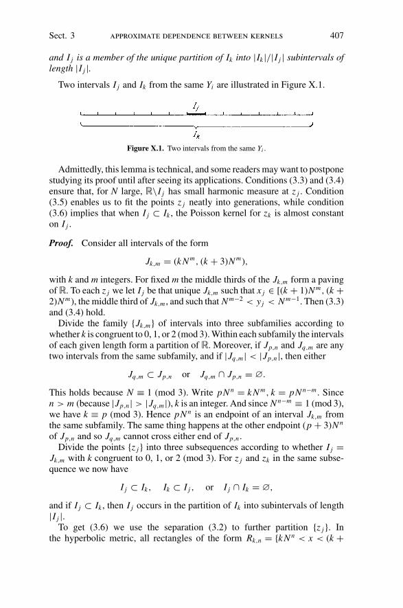
Sect. 3 approximate dependence between kernels 407
and I j is a member of the unique partition of Ik into |Ik |/|I j | subintervals oflength |I j |.
Two intervals I j and Ik from the same Yi are illustrated in Figure X.1.
Figure X.1. Two intervals from the same Yi .
Admittedly, this lemma is technical, and some readers may want to postponestudying its proof until after seeing its applications. Conditions (3.3) and (3.4)ensure that, for N large, �\I j has small harmonic measure at z j . Condition(3.5) enables us to fit the points z j neatly into generations, while condition(3.6) implies that when I j ⊂ Ik , the Poisson kernel for zk is almost constanton I j .
Proof. Consider all intervals of the form
Jk,m = (k N m, (k + 3)N m),
with k and m integers. For fixed m the middle thirds of the Jk,m form a pavingof �. To each z j we let I j be that unique Jk,m such that x j ∈ [(k + 1)N m, (k +2)N m), the middle third of Jk,m , and such that N m−2 < y j < N m−1. Then (3.3)and (3.4) hold.
Divide the family {Jk,m} of intervals into three subfamilies according towhether k is congruent to 0, 1, or 2 (mod 3). Within each subfamily the intervalsof each given length form a partition of �. Moreover, if Jp,n and Jq,m are anytwo intervals from the same subfamily, and if |Jq,m | < |Jp,n|, then either
Jq,m ⊂ Jp,n or Jq,m ∩ Jp,n = ∅.
This holds because N ≡ 1 (mod 3). Write pN n = k N m, k = pN n−m . Sincen > m (because |Jp,n| > |Jq,m |), k is an integer. And since N n−m ≡ 1 (mod 3),we have k ≡ p (mod 3). Hence pN n is an endpoint of an interval Jk,m fromthe same subfamily. The same thing happens at the other endpoint (p + 3)N n
of Jp,n and so Jq,m cannot cross either end of Jp,n .Divide the points {z j } into three subsequences according to whether I j =
Jk,m with k congruent to 0, 1, or 2 (mod 3). For z j and zk in the same subse-quence we now have
I j ⊂ Ik, Ik ⊂ I j , or I j ∩ Ik = ∅,
and if I j ⊂ Ik , then I j occurs in the partition of Ik into subintervals of length|I j |.
To get (3.6) we use the separation (3.2) to further partition {z j }. Inthe hyperbolic metric, all rectangles of the form Rk,n = {k N n < x < (k +
408 interpolating sequences and maximal ideals Chap. X
3)N n, 3N n−5 < y ≤ 3N n−1} are congruent. By (3.2) each such rectangle con-tains at most n1 = n1(α, N ) sequence points z j . Partition each of our three sub-sequences into n1 subsequences so that every rectangle Rk,n contains at mostone point from each subsequence. We then obtain n0 = 3n1, subsequencesY1, . . . , Yn0
for which (3.5) and (3.6) hold.
By (3.5) the points z j in each subsequence Yi , and their corresponding inter-vals I j , fit naturally into generations. When z j , zk ∈ Yi , we say zk ∈ G1(z j ),and Ik ∈ G1(I j ), if Ik � I j and Ik is maximal. Successive generations, as al-ways, are defined inductively:
G p(I j ) =⋃
G p−1(I j )
G1(Ik).
Lemma 3.2. Suppose {z j } is a sequence of points satisfying (3.2). Let N begiven and let Y1, Y2, . . . , Yn0
, n0 = n0(α, N ), be the subsequences given byLemma 3.1. Let 0 < γ < 1 and let r be a positive integer. Then there existsA = A(α, N , γ, r ) such that if (3.1) fails with constant A, that is, if
supQ
∑
z j ∈Q
y j
l(Q)> A,
then there is a subsequence Yi and a point z j ∈ Yi such that
∑
Gr (I j )
|Ik ||I j | > γ.
In a quantative way, this lemma says that to establish (3.1) it is enough towork with the special sequences Yi .
Proof. If the contrary holds, then for every Yi and for every z j ∈ Yi , inductiongives
∑
Gq (I j )
|Ik ||I j | ≤ γ n,
when nr ≤ q < (n + 1)r . Consequently,
∑
Ik ⊂I jzk ∈Yi
|Ik ||I j | ≤ r
1 − γ.
Summing over the Yi then yields
∑
Ik⊂I
|Ik ||I | ≤ n0r
1 − γ,
and since yk/|Ik | is bounded above and below, this proves that (3.1) holds withsome constant A = A(α, N , γ, r ).
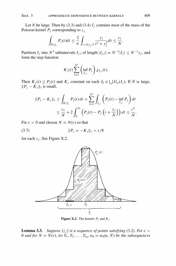
Sect. 3 approximate dependence between kernels 409
Let N be large. Then by (3.3) and (3.4) I j contains most of the mass of thePoisson kernel Pj corresponding to z j
∫
�\I j
Pj (t)dt ≤ 2
π
∫
t>N y j /3
y j
t2 + y2j
dt ≤ c1
N.
Partition I j into N 3 subintervals I j,l of length |I j,l | = N−3|I j | ≤ N−1 y j , andform the step function
K j (t)N 3∑
l=1
(
infI j,l
Pj
)
χI j,l (t).
Then K j (t) ≤ Pj (t) and K j constant on each Ik ∈ ⋃Gq (I j ). If N is large,
‖Pj − K j‖1 is small,
‖Pj − K j‖1 ≤∫
�\I j
Pj (t) dt +N 3∑
l=1
∫
I j,l
(
Pj (t) − infI j,l
Pj
)
dt
≤ c1
N+ 2
∫ ∞
0
(Pj (t) − Pj
(t + y j
N
))dt ≤ c2
N.
Fix ε > 0 and choose N = N (ε) so that
‖Pj = −K j‖1 < ε/8(3.7)
for each z j . See Figure X.2.
Figure X.2. The kernels Pj and K j .
Lemma 3.3. Suppose {z j } is a sequence of points satisfying (3.2). For ε >
0 and for N = N (ε), let Y1, Y2 . . . , Yn0, n0 = n0(α, N ) be the subsequences
410 interpolating sequences and maximal ideals Chap. X
given by Lemma 3.1. There exist β = β(ε), 0 < β < 1, and a positive integerp = p(ε) such that if
∑
G p(I j )
|Ik ||I j | ≥ β(3.8)
for some point z j ∈ Yi , then there exist convex weight λk, 0 ≤ λk < 1,∑
λk =1 such that
‖Pj − ∑λk Pk‖1 < ε,(3.9)
λk = 0 if zk ∈ G1(z j ) ∪ . . . ∪ G p(z j ),(3.10)
and
λk ≤ b|Ik |/|I j |,(3.11)
where b = b(N ) is a constant.
Proof. We are going to find weights λk satisfying (3.10) and (3.11) such that
0 ≤∑
λk Kk ≤ K j
and such that
‖K j −∑
λk Kk‖1 < ε/8.(3.12)
Replacing λk by λk/∑
λi and using (3.7), we then obtain convex weights forwhich we have (3.9)–(3.11).
Set f0(t) = K j (t). Then f0 has constant value f0(Ik) on each first generationinterval Ik ∈ G1(I j ). These intervals are disjoint and Kk is supported on Ik
Set λk = f0(Ik)/‖Kk‖∞, zk ∈ G1(z1), and f1 = f0 − ∑G1λk Kk . Then 0 ≤
f1 ≤ f0, and f1 has constant value f1(Ik) on each Ik ∈ G2(I j ). Repeat theconstruction using f1 in place of f0 and continue through p generations. Atstage q, fq−1 has constant value fq−1(Ik) on each Ik ∈ Gq (I j ), and we set
λk = fq−1(Ik)/‖Kk‖∞, zk ∈ Gq (z j )
fq = fq−1 −∑
Gq (I j )
λk Kk = K j −q∑
r=1
∑
Gr (I j )
λk Kk .
Then 0 ≤ fq ≤ fq−1 ≤ f0. See Figure X.3. By (3.4) we have fq−1(Ik) ≤‖ f0‖∞ ≤ c1/|I j | while by (3.3) and (3.4), ‖Kk‖∞ ≥ c2/|Ik |. Hence λk ≤b|Ik |/|I j | and (3.11) holds. We have (3.10) because the process is stoppedwhen f p has been constructed.
It remains to estimate‖K j − ∑λk Kk‖1 = ∫
f p dt . Since‖Kk‖∞ ≥ c2/|Ik |,(3.7) yields
∫Kk
‖Kk‖∞dt ≥ (1 − ε)|Ik |
c2
= (1 − δ)|Ik |,

Sect. 3 approximate dependence between kernels 411
Figure X.3. For each Ik ∈ Gq , λk Kk ≤ fq−1(Ik ), but∫
Ikλk Kkdt ≥ δ
∫Ik
fq−1dt .
with 0 < δ < 1. Consequently, when Ik ∈ Gq we have∫
fq dt = |Ik | fq−1(Ik) − fq−1(Ik)
∫Kk
‖Kk‖∞dt
≤ δ|Ik | fq−1(Ik) = δ
∫
Ik
fq−1 dt.
Let E0 = I j , Eq = ⋃Gq
Ik, q = 1, 2, . . . , p. Then E0 ⊃ E1 ⊃ . . . ⊃ E p, and
induction yields∫
E p
f p dt ≤ δ
∫
E p
f p−1 dt ≤ δ
∫
E p−1
f p−1 dt
≤ δ p∫
E0
f0 dt ≤ δ p.
Choose p so that δ p < ε/16. Recall that ‖ f p‖∞ ≤ ‖ f0‖∞ ≤ c1/|I j |, where c1
depends only on ε. Our hypothesis is that |E p|/|I j | ≥ β, for some β = β(ε)yet to be determined. Now choose β = β(ε) so that (1 − β)c1 < ε/16. Thenwe obtain ‖ f0‖∞|I j\E p| < ε/16 and
∫f p dt ≤ δ p +
∫
I j\E p
f p dt ≤ δ p + ‖ f0‖∞|I j\E p| < ε/8,
so that (3.12) holds.
Theorem 3.4. Let {z j } be a sequence in the upper half plane. Assume thereare real valued harmonic functions {u j (z)} such that
(i) ‖u j‖∞ ≤ 1,(ii) u j (z j ) ≥ δ > 0,
(iii) u j (zk) ≤ 0, k = j ,
where δ > 0 is independent of j. Then {z j } is an H∞ interpolating sequence.
The hypothesis of the theorem is reminiscent of the condition
infj
∏
k;k = j
∣∣∣∣z j − zk
z j − zk
∣∣∣∣ = δ > 0

412 interpolating sequences and maximal ideals Chap. X
characterizing interpolating sequences, but there seems to be no direct deriva-tion of this condition from the theorem’s hypothesis. Note that the theoremgeneralizes Theorem 4.2 of Chapter VII.
Proof. Clearly, the points are separated. The bounded function exp(u j + i u j )separates z j from each other zk . We claim (3.1) holds. That will prove thetheorem. If (3.1) fails, then by Lemmas 3.2 and 3.3 there is a point z j and thereare weights λk ≥ 0, λ j = 0, such that ‖Pj − ∑
λk Pk‖1 < δ. But then
δ ≤ u j (z j ) −∑
λku j (zk) =∫
u j (Pj −∑
λk Pk) dt
≤ ‖u j‖∞‖Pj −∑
λk Pk‖1 < δ,
a contradiction.
Lemma 3.3 and Theorem 3.4 are also true with approximate identities moregeneral than the Poisson kernel (see Exercise 12).
4. Interpolating Sequences and Harmonic Separation
We continue the discussion of the preceding section. Our objective is anothercharacterization of interpolating sequences.
Theorem 4.1. Let {z j } be a sequence in the upper half plane. Then {z j } isan interpolating sequence if disjoint subsets of {z j } have disjoint closures inthe maximal ideal space M of H∞.
Before getting into its proof, let us see what this theorem means. Noticethat the converse of the theorem is trivial. Is S and T are disjoint subsets ofan interpolating sequence, then there is f ∈ H∞ such that f (z j ) = 0 whenz j ∈ S and f (z j ) = 1 when z j ∈ T . With respect to M, the closures of S andT lie in the disjoint closed sets { f = 0} and { f = 1} respectively. If we makethe additional assumption that the closure K of {zn} in M is a hull (i.e., ifm ∈ M\K , there is f ∈ H∞ such that f (m) = 0 but f ≡ 0 on K), then thetheorem follows from a general result of Silov and Exercise 8 of Chapter VII(see Hoffman [1962a]).
As we saw in Chapter V, M is homeomorphic to a weak-star compact subsetof the dual space (L∞)∗, and under that homeomorphism z j corresponds toits Poisson kernel Pj . Hence the hypothesis of the theorem is that disjointsubsets of {Pj } have disjoint weak-star closures in (L∞)∗. This hypothesis canbe reformulated two ways. First, it means that the weak-star closure of {Pj }in (L∞)∗ is homeomorphic to β�, the Stone-Cech compactification of theintegers. Equivalently, the closure of {z j } in M is homeomorphic to β�. Thus{z j } is an interpolating sequence if and only if its closure inM is homeomorphicto β�.

Sect. 4 interpolating sequences and harmonic separation 413
Secondly, every basic weak-star open subset V of (L∞)∗ is defined by areal number α and by finitely many functions u1, u2, . . . , uM ∈ L∞ in thefollowing way:
V = Vα = {ϕ ∈ (L∞)∗ : ϕ(um) < α, 1 ≤ m ≤ M}.
Let S and T be subsets of {Pj } having disjoint weak-star closures in (L∞)∗. Eachpoint ϕ ∈ S, the weak-star closure of S, has a neighborhood Vα such that Vα ∩T = ∅. Since T is compact there is β > α such that Vβ ∩ T = ∅. Sinceϕ(1) =1 when ϕ ∈ S ∪ T , we can take α = −1 and β > 1 by replacing each um byaum + b, a and b constants. Covering S by finitely many such neighborhoods
V (n)−1 , 1 ≤ n ≤ K , we arrive at the following equivalent formulation of the
hypothesis:Whenever S and T are disjoint subsets of {z j }, there are {u(n)
m } ∈ L∞, 1 ≤n ≤ K , 1 ≤ m ≤ M such that
infn
supm
u(n)m (z j ) ≤ −1 i f z j ∈ S,
infn
supm
u(n)m (z j ) > +1 i f z j ∈ T .
(4.1)
Taking K = M = 1 in (4.1), we see that Theorem 4.1 also generalizes Theorem4.2 of Chapter VII. Roughly speaking, Theorem 4.1 says that a sequencesatisfies (3.1) and (3.2) if any reasonable form of separation is possible withbounded harmonic functions.
The proof of the theorem will focus on the concrete condition (4.1). It willbe crucial that the numbers K , M , and
B = supn,m
‖u(n)m ‖∞
can be chosen not to depend on the subsets S and T of {z j }.Lemma 4.2. If disjoint subsets of {z j } have disjoint closures in M, then (4.1)holds with K, M, and B = supn,m ‖u(n)
m ‖∞ not depending on the subsets S andT of {z j }.Proof. We can suppose T = {z j }\S. The set L of all subsets S of {z j } is acompact space in the product topology, in which a neighborhood V of a subsetS0 is determined by finitely many indices j1, j2, . . . , js by the rule
V = V (S0; j1, j2, . . . , js) = {S ∈ L : z jl ∈ S ⇔ z jl ∈ S0, 1 ≤ l ≤ s}.
For K , M , and B positive integers, let EK ,M,B = {S ∈ L : (4.1) holds withbounds K , M , and B}. Then L = ⋃
EK ,M,B , and by normal families each setEK ,M,B is closed in the product topology of L . By the Baire category theo-rem, some EK ,M,B contains an open set V (S0; j1, j2, . . . , js). By the definition

414 interpolating sequences and maximal ideals Chap. X
of the product topology this means that except for the finitely many pointsz j1, z j2, . . . , z js , we have (4.1) with bounds on K , M , and B that do notdepend on the subsets S and T. Adjoining finitely many additional func-tions u(n)
m to separate z j1, z j2, . . . , z js , we then obtain (4.1) with uniformbounds.
We prove Theorem 4.1 using Lemma 3.3 and an iteration. Afterward weshall indicate how an alternate proof can be based on Theorem 6.1 of ChapterVIII.
Proof of Theorem 4.1. By Lemma 4.2 the points z j are separated, and (3.2)holds withα = α(B). The problem now is to derive the Carleson condition (3.1)from (4.1). Let ε = (4BK )−1, and take N = N (ε), p = p(ε), and β = β(ε)in accordance with Lemma 3.3. Here is the strategy. If (3.1) fails, then asubsequence Yi contains a point z0 such that
∑
Gr (z0)
|Ik ||I0| > γ
with r = 2(BK + 1)p and with 1 − γ very small. This will mean that we have(3.9) for z j in a large portion of Gq for a large number of indices q. When thesubsets S and T are chosen properly, this will contradict Lemma 4.2.
If there were ρ < 1 and q ≤ 2BK p such that for all Yi , and all z0 ∈ Yi
∑
Gq (z0)
⎧⎨
⎩|I j ||I0| :
∑
G2 p(z j )
|Ik ||I j | < β
⎫⎬
⎭> ρ,(4.2)
then
∑
Gq+2p(z0)
|Ik ||I0| < ρβ + (1 − ρ)
for all z0 in all Y j . By Lemma 3.2 we should then have (3.1).Assume (4.2) fails for a fixed point z0 ∈ Yi , for all q ≤ 2BK p and for ρ < 1
to be determined. Choose subsets S and T of {z j } so that z0 ∈ T and so thatfor sp < q ≤ (s + 1)p, s ≥ 0, G p(z0) = Gq ⊂ S if s is even and Gq ⊂ T if sis odd. Thus we alternate between S and T after every p generations.
Note that (4.1) is unchanged if we permute the indices {1, 2, . . . , K } or if,
for any fixed n, we permute the set of functions {u(n)1 , u(n)
2 , . . . , u(n)M }. So we can
assume u(n)1 (z0) > 1 for 1 ≤ n ≤ K . Let v = ∑K
n=1 u(n)1 . Then ‖v‖∞ ≤ BK ,
but v(z0) ≥ K . By Lemma 3.3 there are convex weights λ j ≥ 0 such that
p∑
1
∑
Gq (z0)
λ jv(z j ) > K − εBK = K − 1
4.
Sect. 4 interpolating sequences and harmonic separation 415
Since |v(z j )| ≤ BK , Chebychev’s inequality (for the measure∑
λ jδz j ) thenyields
p∑
1
∑
Gq (z0)
{λ j : v(z j ) > K − 12} ≥ 1
4BK.
Then by (3.11) there is q1, 1 ≤ q1 ≤ p, and there is E1 ⊂ Gq1, such thatv(z j ) ≥
K − 12
on E1 and such that
∑
E1
|I j ||I0| ≥ 1
bp
1
4BK= δ1,
where b is the constant in (3.11). Assume (4.2) fails with 1 − ρ < δ1/2. Thenthere is F1 ⊂ E1 such that
∑
F1
|I j ||I0| ≥ 1
2δ1,
and for each z j ∈ F1
∑G2p(z j )
|Ik |/|I j | ≥ β.
For z j ∈ F1 ⊂ S, we have (3.9) with weights λk attached only to points inG p+1 ∪ · · · ∪ G2p ⊂ T , because if q1 < p we still have (3.8) when we deleteG1(z j ) ∪ · · · ∪ G p−q1(z j ). (It is for this reason that 2p occurs inside (4.2).)
Fix z j ∈ F1. Then z j ∈ S and we can permute the indices {1, 2, . . . , K }so that u(1)
1 (z j ) < −1. This permutation depends on the point z j ∈ F1, butthat does not harm what we are going to do, because distinct z j ∈ F1 have
disjoint generations⋃
Gq (z j ). set v′ = v − u(1)1
∑K2 u(n)
1 . Then ‖v′‖∞ < BKbut v′(z j ) > K + 1
2. We have convex weights λk such that
2p−q1∑
p−q1+1
∑
Gq (z j )
λkv′(zk) > K + 1
4,
and Chebychev’s inequality now yields
2p−q1∑
p−q1+1
∑
Gq (z j )
{λk : v′(zk) > K } ≥ 1
4BK.
Arguing as before using (3.11), we have q1(z j ), p < q1(z j ) ≤ 2p, andE1(z j ) ⊂ Gq1(z j ) such that v′(zk) > K on E1(z j ) and such that
∑
E1(z j )
|Ik ||I j | ≥ δ1.

416 interpolating sequences and maximal ideals Chap. X
Summing over F1, we find there is an index q2, p < q2 ≥ 2p, and a setE2 ⊂ Gq2
such that
∑
E2
|Ik ||I0| ≥ δ1
p
∑
F1
|I j ||I0| ≥ δ2
1
2p= δ2,
and such that for each zk ∈ E2v′(zk) > K (after a suitable permutation of
{1, 2, . . . , K }). We assume (4.2) fails with 1 − ρ < δ2/2. Then we have F2 ⊂E2 such that
∑
F2
|Ik ||I0| ≥ δ2
2
and such that for each zk ∈ F2,∑
G2p(zk ) |I j |/|Ik | ≥ β.
Moreover, since F2 ⊂ T , for each zk ∈ F2 we can permute the set
{u(1)1 , u(1)
2 , . . . , u(1)m } so that u(1)
1 (zk) > 1. Then v(zk) = ∑kn=1 u(n)
1 (zk) > K +1. If (4.2) fails with 1 − ρ small enough, we can repeat the above argumentreplacing z0 by each zk ∈ F2 and obtain a set F4 ⊂ Gq4
⊂ T such that
∑
F4
|I j ||I0| ≥ 1
2δ4
for some δ4 = δ4(δ2, p) and such that (after suitable permutations of u(n)m )
v(z j ) > K + 2, z j ∈ F4.Now if (4.2) fails with 1 − ρ extremely small, we can do the above ar-
gument (B − 1)K times. We then reach a point zk for which, after theappropriate permutations of {u(n)
m }, v(zk) > BK . This contradiction provesTheorem 4.1.
To derive Theorem 4.1 from Theorem 6.1 of Chapter VIII, partition the tophalf of each dyadic square Q = {k2−n ≤ x ≤ (k + 1)2−n, 0 < y ≤ 2−n} into22N−1 small squares Sj of side 2−n−N , If B = supm,n ‖u(n)
m ‖∞ is the boundguaranteed by Lemma 4.2, choose N so that
supz,w∈Sj
|u(z) − u(w)| ≤ 1
2(4.3)
whenever u(z) is harmonic and ‖u‖∞ ≤ B.
Fix a dyadic square Q. The first generation G1 = {S(1)j } consists of those
small squares Sj ⊂ Q such that S(1)j contains a sequence point z(1)
j but such
that S(1)j lies below no other small square in Q having the same property. Choose
one sequence point z(1)j in each S(1)
j and let F1 = {z(1)j }. Let Q(1)
j be the dyadic
square having base the projection of S(1)j onto {y = 0}. Then the dyadic squares
Q(1)j have pairwise disjoint interiors.

Sect. 4 interpolating sequences and harmonic separation 417
Inside each Q(1)j select small squares S(2)
k in the same way. Write G1(S(1)j )
and
G2 =⋃
{G1(S(1)j ) : S(1)
j ∈ G1}.Choose one sequence point z(2)
k ∈ S(2)k and set F2 = {z(2)
k : S(2)k ∈ G2}. Form
new dyadic squares {Q(2)k } by dropping the S(2)
k onto the axis. Continue theprocess, obtaining the generations G3, G4, . . . , and the corresponding subsetsF3, F4, . . . , of the original sequence {z j }.
By Lemma 4.2, the points {z j } are separated. If R(p)k is the rectangle, with
sides parallel to the axes, joining the top edge of Q(1)k to the top edge of S(p)
k ,then because the points are separated,
∑
z j ∈R(p)k
y j ≤ C1�(S(p)k ).
Consequently, {z j } is an interpolating sequence if and only if
∞∑
p=1
∑
G p
l(S(p)k ) ≤ C2�(Q)(4.4)
for each dyadic square Q lying on {y = 0}. Because∑
G1�(S(1)
j ) ≤ �(Q), we
only need to estimate∑∞
2 in (4.4).Replace {z j } by the subsequence F1 ∪ F2 ∪ · · · . This does not change the
sum (4.4). Partition {z j } by setting
S =⋃
{Fp : p odd}, T =⋃
{Fp : p even}.Then by (4.1) and (4.3) there exist finitely many bounded harmonic functions
u(n)m such that whenever S(p)
k ∈ G1(S(p−1)j ),
inf
{
maxm,n
|u(n)m (z) − u(n)
m (w)| : z ∈ S(p)k , w ∈ S(p−1)
j
}
≥ 1.
By Theorem 6.1 of Chapter VIII, there exist smooth functions ϕ(n)m (z) such that
inf
{
maxm,n
|ϕ(n)m (z) − u(n)
m (w)| : z ∈ S(p)k , w ∈ S(p−1)
j
}
≥ 12,(4.5)
and such that∫∫
Q
∑
m,n
|∇ϕ(n)m |dxdy ≤ C3�(Q)(4.6)
for each square Q resting on {y = 0}.Let S(p)
k ∈ G p, p ≥ 2. Then S(p)k ∈ G1(S(p−1)
j ) for some S(p−1)j ∈ G p−1 and
S(p)k lies below S(p−1)
k . Let T (p)k be the rectangle, with sides parallel to the axes,

418 interpolating sequences and maximal ideals Chap. X
Figure X.4. Theorem VIII.6.1 implies Theorem 4.1.
joining the top edge of S(p)k to the same dyadic interval on the bottom edge of
S(p−1)j . The rectangles {T (p)
k } have pairwise disjoint interiors. See Figure X.4.By (4.5),
∑
m,n
∫∫
T (p)k
|∇ϕ(n)m |dx dy ≥ max
m,n
∫∫
T (p)k
∣∣∣∣∂ϕ(n)
m
∂y
∣∣∣∣ dx dy
≥ 12�(S(p)
k ),
and since the rectangles T (p)k are disjoint, (4.4) now follows from (4.6).
Of the two proofs of Theorem 4.1, the second one looks more transparent,but it is not perfectly clear which argument is stronger. For example, Theorem3.4 does not seem to follow from Theorem VIII.6.1.
5. A Constructive Douglas–Rudin Theorem
Theorem 5.1. Suppose u ∈ L∞, |u| = 1 almost everywhere. Let ε < 0. Thenthere exist interpolating Blaschke products B1(z) and B2(z) such that
‖u − B1/B2‖∞ < ε.
Sect. 5 a constructive douglas–rudin theorem 419
This result refines the Douglas–Rudin theorem, Chapter V, Section 2. Beforeproving the theorem, we mention one corollary and two related open problems.
Corollary 5.2. The interpolating Blaschke products separate the points ofthe maximal ideal space M of H∞.
Proof. Let m1 and m2 be distinct points of M. There are three cases.
Case 1. m1 ∈ X and m2 ∈ X , where X = ML∞ is the Silov boundary ofH∞. By Theorem 5.1, L∞ is the self-adjoint closed algebra generated bythe interpolating Blaschke products. Consequently the interpolating Blaschkeproducts separate the points of X = ML∞ .
In the remaining two cases we have m1 ∈ M\X or m2 ∈ M\X . By sym-metry we can suppose m1 ∈ M\X . Recall the notation
G = {m ∈ M : m is in the closure of an interpolating sequence}.
Case 2. m1 ∈ G. Then there is an interpolating Blaschke product B(z) suchthat B(m1) = 0. If also B(m2) = 0, then m1, and m2 are in the closure ofthe zeros S of B(z), and there are disjoint subsets T1 and T2 of S such thatm1 ∈ T1, m2 ∈ T2. The Blaschke product with zeros T1 then separates m1 andm2. (See, for instance, the conclusion of the proof of Theorem 1.7.)
Case 3. m1 ∈ X ∪ G. Then m1 and m2 are in different Gleason parts. Forevery ε > 0 there is fε ∈ H∞ such that fε(m1) = 0, | fε(m2)| > 1 − ε, and‖ fε‖ = 1. By Corollary 2.6 of Chapter V, there is an inner function uc ∈ H∞such that uε(m1) = 0 and |uε(m2)| > 1 − ε. By Theorem 4.1 of Chapter VIII,there is an interpolating Blaschke product Bε(z) such that
|Bε(z)| < 14
if |uε(z)| < 14,(5.1)
|uε(z)| < β if Bε(z) = 0,(5.2)
where β = β(
14
)is some constant. Moreover,
δ(Bε) ≥ δ0,(5.3)
where δ0 > 0 is a constant independent of ε. Now we claim there is η(ε) →0(ε → 0) such that
|Bε(z)| ≥ 1 − η(ε) if |uε(z)| ≥ 1 − ε.(5.4)
Accepting (5.4) for the moment, we choose ε so small that 1 − η(ε) ≥ 12.
Then by (5.1) and the corona theorem, Bε(m1) ≤ 14, while by (5.4) and the
corona theorem, |Bε(m2)| ≥ 12. Thus the interpolating Blaschke product Bε
separates m1 and m2.
420 interpolating sequences and maximal ideals Chap. X
To prove (5.4), we use some ideas from Section 3, Chapter VIII. Suppose|uε(z)| > 1 − ε. Using a Mobius transformation, we can assume z = 0. Let
Eβ ={
θ : inf�(θ )
|uε(z)| < β
}
,
where �(θ ) denotes the cone
�(θ ) ={
z :|z − eiθ |1 − |z| < 2
}
.
Write v(θ ) = |uε(eiθ ) − uε(0)|2. Then∫
v(θ )dθ/2π = 1 − |uε(0)|2 < 2ε,whereas if |uε(z)| < β, then
1
2π
∫v(θ )Pz(θ )dθ ≥ |uε(z) − uε(0)|2 ≥ (1 − ε − β)2.
The weak-type estimate for the nontangential maximal function thereforeyields
|Eβ | ≤ 2cε
(1 − ε − β)2.(5.5)
Write Eβ = ⋃I j , where the I j are pairwise disjoint ares on ∂D and set
Sj = {reiθ : θ ∈ I j , 1 − |I j | < r < 1}.By (5.2) the zeros {zn} of Bε(z) lie inside
⋃Sj . Hence by (5.3) and (5.5)
∑(1 − |zn|) ≤ C(δ0)
2cε
(1 − ε − β2).
Because β = β(
14
)fixed we conclude that |Bε(0)| ≥ 1 − η(ε), where η(ε) →
0(ε → 0). That establishes (5.4).
Problem 5.3. Do the interpolating Blaschke products generate H∞ as auniform algebra?
Problem 5.4. Can every Blaschke product be uniformly approximated byinterpolating Blaschke products?
Since the Blaschke products generate H∞, a yes answer to Problem 5.4would imply a yes answer to Problem 5.3. See page vii.
The proof of Theorem 5.1 is different from the constructions we have dis-cussed above.
Lemma 5.5. Let ε > 0, δ > 0, and η > 0. Suppose I1, I2, . . . , IK are pair-wise disjoint closed bounded intervals on �, and suppose α1, α2, . . . , αK arereal numbers, 0 < α j < 2π . Then there exist finite Blaschke products B1(z)
Sect. 5 a constructive douglas–rudin theorem 421
and B2(z), having simple zeros, such that∑
j
|{x ∈ I j : |α j − ArgB1(x)/B2(x)| ≥ ε/2}| < η.(5.6)
and such that
0 < Arg B1(x)/B2(x) < δ x ∈⋃
I j .(5.7)
The zeros {zn} of B1(z) or of B2(z) satisfy
ρ(zn, zm) ≥ cε, n = m,(5.8)
with c some absolute constant, and
xn = Re zn ∈⋃
j
I j .(5.9)
Moreover, if 0 < y < y0(ε, δ, K ), then the zeros zn may be chosen on thehorizontal line
yn = Im zn = y.
Here Arg w denotes the principal branch of the argument, 0 ≤ Arg w < 2π .
Proof. Because the intervals are pairwise disjoint, it is enough to prove thislemma for one interval I (with η replaced by η/K , with ε replaced by ε/2, andwith δ replaced by min(δ/K , ε/2K )). Fix a closed interval I. After a translationwe can suppose
I = [−η/4, A + η/4].
Also fix α, 0 < α < 2π .Let N be a positive integer, to be determined later, and consider the points
xk = k/N , 0 ≤ k ≤ k0 = [N A] − 1,
[t] denoting the greatest integer in t. Let
λ = α/2π N
and fix y > 0, also to be determined later. The zeros of B1(z) are
zk = xk + iy, 0 ≤ k ≤ k0,
and the zeros of B2(z) are
z∗k = xk + λ + iy, 0 ≤ k ≤ k0
See Figure X.5. Because k0/N + λ < A, we have (5.9). We set
B1(z) =k0∏
k=0
z − zk
z − zk, B2(z) =
k0∏
k=0
z − z∗k
z − z∗k
,

422 interpolating sequences and maximal ideals Chap. X
Figure X.5. Here α = 2π/3. The zeros of B2(z) are slightly to the right of the zeros of B1(z).
so that, modulo 2π ,
ArgB1(x)
B2(x)=
k0∑
k=0
(
Arg
(x − zk
x − zk
)
− Arg
(x − z∗
k
x − z∗k
))
.
Note that
Arg
(x − zk
x − zk
)
= π + 2 arctan
(x − xk
y
)
= 2
∫ ∞
xk
yk
(x − t)2 + y2k
dt.
Consequently,
ArgB1(x)
B2(x)= 2
k0∑
k=0
∫ xk+λ
xk
yk
(x − t)2 + y2k
dt.(5.10)
Because the intervals of integration are pairwise disjoint, the right side of(5.10) has value in (0, 2π ) and it is the principal branch of the argument.
Setting E = ⋃k0
k=0[xk, xk + λ], we see that
ArgB1(x)
B2(x)= 2π
∫Py(x − t)χE (t) dt.
Since dist(E, �\I ) ≥ η/4, (5.10) yields
ArgB1(x)
B2(x)≤ 2
∫ ∞
η/4
y ds
s2 + y2≤ c1 y
η, x ∈ I.
Therefore (5.7) will hold if
y ≤ c2 δη.(5.11)
Now let J = [η/4, A − η/4]. Then J ⊂ I and |I\J | = η. We shall have(5.6) if we can get
|α − Arg B1(x)/B2(x)| < ε/2, x ∈ J.(5.12)
As a preliminary approximation set F = [0, xk0+ 1/N ] and write
V (x) = α
n
∫
F
y
(s − t)2 + y2dt.
Taking
N ≥ δ/η,(5.13)

Sect. 5 a constructive douglas–rudin theorem 423
we have xk0+ 1/N ≥ A − 1/N ≥ A − η/8, and dist(J, �\F) > η/8. Thus
as before
|V (x) − α| ≤ δ
π
∫ ∞
η/8
y ds
s2 + y2≤ c3 y
η, x ∈ J ′;
and
|V (x) − α| < ε/4, x ∈ J,
provided that
y ≤ c4εη.(5.14)
But now for any x ∈ �,∣∣∣∣V (x) − Arg
B1(x)
B2(x)
∣∣∣∣ =
∣∣∣∣α
π
∫
F
y
(x − t)2 + y2dt − 2
∫
E
y
(x − t)2 + y2dt
∣∣∣∣
≤k0∑
k=0
∣∣∣∣α
π
∫ xk+1
xk
y dt
(x − t)2 + y2− 2
∫ xk+λ
xk
y dt
(x − t)2 + y2
∣∣∣∣(5.15)
=k0∑
k=0
∣∣∣∣
∫ xk+1
xk
gk(t)y
(x − t)2 + y2dt
∣∣∣∣ ,
where |gk(t)| ≤ 2 and∫ xk+1
xkgk(t)dt = 0. Consequently,
∣∣∣∣
∫ xk+1
xk
gk(t)y
(x − t)2 + y2dt
∣∣∣∣ ≤ 2
Nmax
xk≤t≤xk+1
(y
(x − t)2 + y2
)
− 2
Nmin
xk≤t≤xk+1
(y
(x − t)2 + y2
)
,
and the right side of (5.15) is bounded by a two-sided telescoping sum. There-fore
|V (x) − ArgB1(x)/B2(x)| ≤ 4/N y, 2
and we have (5.12) and also (5.6) if we take
N y = c5/ε.(5.16)
Our restrictions (5.11), (5.13), and (5.14) on the parameters y and N areconsistent with (5.16) and we can obtain (5.6) and (5.7) with arbitrarily smally. Finally, by (5.16)
ρ(zn, zm) ≥ c6|xn − xm |/y ≥ cε, n = m,
and so (5.8) holds.
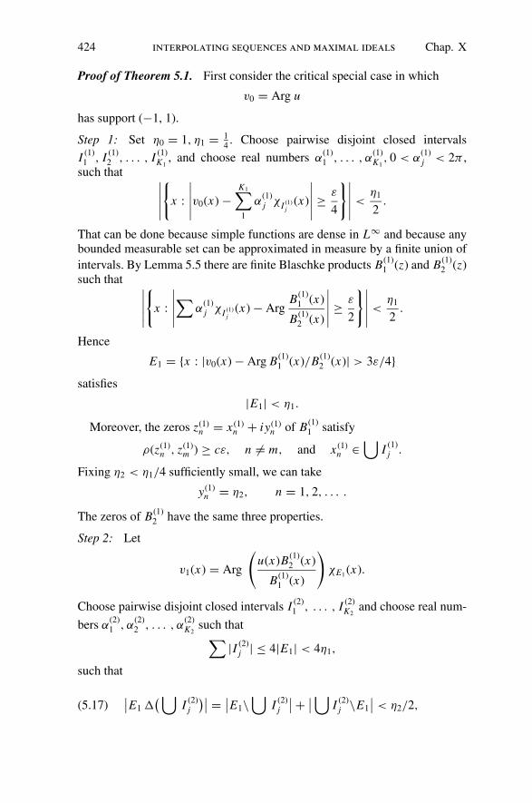
424 interpolating sequences and maximal ideals Chap. X
Proof of Theorem 5.1. First consider the critical special case in which
v0 = Arg u
has support (−1, 1).
Step 1: Set η0 = 1, η1 = 14. Choose pairwise disjoint closed intervals
I (1)1 , I (1)
2 , . . . , I (1)K1
, and choose real numbers α(1)1 , . . . , α
(1)K1
, 0 < α(1)j < 2π ,
such that ∣∣∣∣∣
{
x :
∣∣∣∣∣v0(x) −
K1∑
1
α(1)j χI (1)
j(x)
∣∣∣∣∣≥ ε
4
}∣∣∣∣∣<
η1
2.
That can be done because simple functions are dense in L∞ and because anybounded measurable set can be approximated in measure by a finite union of
intervals. By Lemma 5.5 there are finite Blaschke products B(1)1 (z) and B(1)
2 (z)such that ∣
∣∣∣∣
{
x :
∣∣∣∣∣
∑α
(1)j χI (1)
j(x) − Arg
B(1)1 (x)
B(1)2 (x)
∣∣∣∣∣≥ ε
2
}∣∣∣∣∣<
η1
2.
Hence
E1 = {x : |v0(x) − Arg B(1)1 (x)/B(1)
2 (x)| > 3ε/4}satisfies
|E1| < η1.
Moreover, the zeros z(1)n = x (1)
n + iy(1)n of B(1)
1 satisfy
ρ(z(1)n , z(1)
m ) ≥ cε, n = m, and x (1)n ∈
⋃I (1)
j .
Fixing η2 < η1/4 sufficiently small, we can take
y(1)n = η2, n = 1, 2, . . . .
The zeros of B(1)2 have the same three properties.
Step 2: Let
v1(x) = Arg
(u(x)B(1)
2 (x)
B(1)1 (x)
)
χE1(x).
Choose pairwise disjoint closed intervals I (2)1 , . . . , I (2)
K2and choose real num-
bers α(2)1 , α
(2)2 , . . . , α
(2)K2
such that∑
|I (2)j | ≤ 4|E1| < 4η1,
such that
∣∣E1 �
( ⋃I (2)
j
)∣∣ = ∣∣E1\
⋃I (2)
j
∣∣ + ∣
∣⋃
I (2)j \E1
∣∣ < η2/2,(5.17)

Sect. 5 a constructive douglas–rudin theorem 425
and such that∣∣∣{
x : |v1(x) −∑
α(2)j χI (2)
j(x)| >
ε
8
}∣∣∣ ≤ η2
4.(5.18)
By Lemma 5.5 there are finite Blaschke products B(2)1 (z) and B(2)
2 (z) such that∣∣∣∣∣
{
x :
∣∣∣∣∣
∑
j
α(2)j χI (2)
j(x) − Arg
B(2)1 (x)
B(2)2 (x)
∣∣∣∣∣>
ε
2
}∣∣∣∣∣<
η2
4,(5.19)
and such that
0 < Arg B(2)1 (x)/B(2)
2 (x) < ε/8, x /∈⋃
I (2)j .(5.20)
Consider the set
E2 ={
x :
∣∣∣∣∣v0(x) − Arg
(B(1)
1 (x)B(2)1 (x)
B(1)2 (x)B(2)
2 (x)
)∣∣∣∣∣>
7ε
8
}
.
Then
E2 = [E2 ∩ E1 ∩ (⋃
I (2)j )] ∪ [E2\(E1 ∪ ⋃
I (2)j )]
∪[E2 ∩ (E1 �(⋃
I (2)j ))]
On E1 ∩ (⋃
I (2)j ), (5.18) and (5.19) give us, modulo 2π ,
∣∣∣∣∣v0(x) − Arg
(B(1)
1 (x)B(2)1 (x)
B(1)2 (x)B(2)
2 (x)
)∣∣∣∣∣=
∣∣∣∣∣v1 − Arg
(B(2)
1 (x)
B(2)2 (x)
)∣∣∣∣∣
<ε
8+ ε
2= 5ε
8,
except on a set of measure at most η2/2 Hence,∣∣∣E2 ∩ E1 ∩
(⋃I (2)
j
)∣∣∣ < η2/2
By (5.20), we have
E2\(⋃
I (2)j
)⊂ E1.
so that
E2\(
E1 ∪⋃
I (2)j
)= ∅.
And by (5.17), we have∣∣∣E2 ∩
(E1�
(⋃I (2)
j
))∣∣∣ < η2/2.
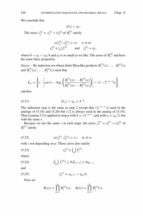
426 interpolating sequences and maximal ideals Chap. X
We conclude that
|E2| < η2.
The zeros z(2)n = x (2)
n + iy(2)n of B(2)
1 satisfy
ρ(z(2)n , z(2)
m ) ≥ cε, n = m,
x (2)η ∈ ⋃
I (2)i and y(2)
n = η3,
where 0 < η3 < η2/4 and η3 is as small as we like. The zeros of B(2)2 and have
the same three properties.
Step p: By induction we obtain finite Blaschke products B(1)1 (z), . . . , B(p)
1 (z)
and B(1)2 (z), . . . , B(p)
2 (z) such that
E p ={
x :
∣∣∣∣∣v0(x) − Arg
(B(1)
1 (x) · · · B(p)1 (x)
B(1)2 (x) · · · B(p)
2 (x)
)∣∣∣∣∣> (1 − 2−p−1)ε
}
satisfies
|E p| < ηp ≤ 4−p.(5.21)
The induction step is the same as step 2 except that ε2−p−1 is used in theanalogs of (5.18) and (5.20) but ε/2 is always used in the analog of (5.19).Thus Lemma 5.5 is applied at step p with δ = ε2−p−1, and with η = ηp/2, butwith the same ε.
Because we use the same ε at each stage, the zeros z(p)n = x (p)
n + iy(p)n of
B(p)1 satisfy
ρ(z(p)n , z(p)
m ) ≥ cε, m = n,(5.22)
with c not depending on p. These zeros also satisfy
x (p)n ∈
⋃I (p)
j ,(5.23)
where
|⋃
I (p)j | ≤ 4|E p−1| ≤ 4ηp−1(5.24)
and
y(p)n = ηp+1 < ηp/4.(5.25)
Now set
B1(z) =∞∏
p=1
B(p)1 (z), B2(z) =
∞∏
p=1
B(p)2 (z).

Sect. 5 a constructive douglas–rudin theorem 427
Because the zeros remain in a bounded set, convergence factors are unnecessaryand the products converge if their assigned zeros satisfy
∑yn < ∞. We show
more: The zeros given to B1(z) (and to B2(z)) are an interpolating sequence.
We consider B1(z) only. It has zeros⋃∞
p=1{z(p)n }. By (5.22) and (5.25) these
zeros are separated. Let Q be a square {a < x < a + h, 0 < y < h}. Since
y(p)n ≤ η2, we can assume h < η2. Take q so that
ηq+1 ≤ h < ηq .
Then by (5.25),
∑
z(p)n ∈Q
y(p)n =
∞∑
p=q
ηp+1 Np(Q),
where Np(Q) is the number of z(p)n inside Q. By (5.22) and (5.25),
|x (p)n − x (p)
m | ≥ c1εηp+1,
so that by (5.23) and (5.24),
Np(Q) ≤ min(| ⋃ I (p)j |, h)
c1εηp+1
≤ c2 min(4ηp−1, h)
εηp+1
.
Therefore, as ηp ≤ 4−p,
∑
z(p)n ∈Q
y(p)n ≤ c2
ε
∞∑
p=q+2
min(4ηp−1, h) ≤ 2c2
εh + c2
ε
∞∑
p=q+2
4ηp−1
≤ c3
εh
∞∑
k=0
4−k,
and⋃ {z(p)
n } is an interpolating sequence. Thus B1(z) and B2(z) are interpo-lating Blaschke products.
In L2(dx/(1 + x2)), the partial products (B(1)1 · · · B(p)
1 · · · B(p)1 )/(B(1)
2 · B(p)2
converge to B1/B2. So a subsequence of the partial products converges toB1/B2 almost everywhere. Hence by (5.21),
|v0(x) − Arg B1(x)/B2(x)| ≤ ε
almost everywhere.For the general case write u = u1u2, where
u1(x) = 1, |x | > 1,
u2(x) = 1, |x | < 1.

428 interpolating sequences and maximal ideals Chap. X
By the special case treated above we have interpolating Blaschke productsB1,1(z) and B2,1(z) such that
∣∣∣∣u1 − B1,1(x)
B2,1(x)
∣∣∣∣ <
ε
2
almost everywhere. Using the inversion z → −1/z, we also get interpolatingBlaschke products B1,2(z) and B2,2(z) such that
∣∣∣∣u2(x) − B1,2(x)
B2,2(x)
∣∣∣∣ <
ε
2
almost everywhere. The theorem will be proved if it can be arranged thatB1 = B1,1 B1,2 and B2 = B2,1 B2,2 are interpolating Blaschke products. Forthat it is enough to bound below the pseudohyperbolic distance from the zerosof B j,1 to the zeros of B j,2, j = 1, 2. The zeros of B1,1 and B2,1 lie in |x | < 1and on horizontal lines y = ηp, p = 2, 3, . . . , with ηp+1 < ηp/4. The zerosof B1,2 and B2,2 lie in |x | > 1 and in large circles tangent to � at z = 0. In{y ≤ η2} these circles cut the lines {x = ±1} at heights y = yq , q = 1, 2, . . . .By Lemma 5.5, we can take y1 and yq+1/yq as small as we please. Thus wecan ensure that
infp
|yq − ηq |yq
≥ cε, q = 1, 2, . . . ,
which implies that the zeros of B1(z) and of B2(z) are interpolatingsequences.
Notes
Sections 1 and 2 are taken from Hoffman [1967]. Further results from his pa-per are given in Exercises 1–8. Lemma 3.3 is due to Carleson [1972]. Theorem4.1 is from Carleson and Garnett [1975], who also study harmonic interpola-tion in �d+1
+ . Theorem 5.1 is in Jones [1981]. The idea behind Lemma 5.5 isdue to A. M. Davie (see Davie, Gamelin, and Garnett [1973]).
Exercises and Further Results
1. Let m ∈ M.
(a) We say m is a nontangential point if m is in the closure of some cone
�α(eiθ ) ={
z :|z − eiθ |1 − |z| < α, |z| < 1
}
,
α > 1. Every nontangential point m is in the closure of an interpolating se-quence, Consequently, m lies in an analytic disc. (Hint: There are finitely manyinterpolating Blaschke products B1, . . . , BN and there is r > 0, r < r (δ(B j ))

exercises and further results 429
(see Lemma 1.4), such that
�α(eiθ ) ⊂N⋃
j=1
{z : ρ(z, z j,k) < r},
where {z j,k} denotes the zeros of B j .)(b) We say m is an orocycular point if m lies in the closure of the region be-
tween two circles tangent to the unit circle at the same point. Every orocycularpoint lies in the closure of an interpolating sequence.
(c) Let r (θ ) be continuous and decreasing on 0 ≤ θ ≤ 1, r (0) = 1, and letγ be the curve {r (θ )eiθ : 0 < θ ≤ 1}, terminating at z = 1. If m ∈ M is in theclosure of γ , then m lies in an analytic disc.
2. Let V be a disc in D tangent to the unit circle at one point eiθ , and letV be the closure of V in M.
(a) V is disjoint from the Silov boundary X.(b) There exist points m ∈ V not in the closure of any interpolating se-
quence. (Otherwise, for any ε > 0 we could, by compactness, cover V bypseudohyperbolic discs {ρ(z, z j ) < ε} with {z j } a finite union of interpolatingsequences, thereby violating the geometric characterization of interpolatingsequences.)
(c) Thus there are one-point Gleason parts disjoint from the Silov boundary.(d) Part (b) and Exercise 1 can be generalized. Let S be any subset of D, and
let {z j } be any separated sequence in S such that⋃{z : ρ(z, z j ) < 1
2} covers
S. Then every point in the closure of S lies in an analytic disc if and only if∑(1 − |z j |)δz j is a Carleson measure.
In the upper half plane, let Qn, j = { j2−n ≤ x ≤ ( j + 1)2−n, 2−n−1 ≤ y ≤2−n}, −∞ < n < ∞, −∞ < j < ∞. Thus {Qn, j } is a paving of H by hy-perbolically congruent rectangles. Let S be a subset of H and consider thesequence {zk} consisting of the centers of those Qn, j such that Qn, j ∩ S = Ø.Every point in the closure of S lies in an analytic disc if and only if {zk} is aninterpolating sequence.
3. The mapping z → Lz from D into MD has a unique continuousextension to a mapping L from M into MD . If m ∈ G, the extension has valueLm . If m /∈ G, then Lm(ζ ) = m, ζ ∈ D .
4. Let CM denote the complex algebra of bounded continuous functionson D which admit continuous extensions to M.
(a) CM is the smallest uniformly closed algebra containing H∞ and H∞.(b) CM is the smallest uniformly closed algebra containing the bounded
harmonic functions.(c) If f ∈ H∞ and if α ∈ D, then
g(z) = f
(α + z
1 + zα
)
∈ CM,

430 interpolating sequences and maximal ideals Chap. X
and for n = 1, 2, . . . ,
hn(z) = (1 − |z|2)n f (n)(z) ∈ CM.
5. Let S ⊂ D and suppose that for some ε, 0 < ε < 1, the ε pseudohy-perbolic neighborhood of S, {z : infS ρ(z, w) < ε} covers D. Then the closureif S in M contains every point not in the closure of any interpolating sequence.(Use the fact that P(m) = {m} for such a point.)
6. Let m ∈ M. A necessary and sufficient condition for m to be in theclosure of some interpolating sequence is the following. If E and F are subsetsof D and if m ∈ E ∩ F , then ρ(E, F) = inf{ρ(z, w) : z ∈ E, w ∈ F} = 0.
7. Let T be an endomorphism from H∞ into H∞; that is, T is a (bounded)linear operator from H∞ into H∞ satisfying
T ( f g) = T ( f )T (g).
Then there exists an analytic mapping τ : D → D, τ (0) = 0, and there existsa net (zi ) in D such that
T f (z) = limi
f
(τ (z) + zi
1 + ziτ (z)
)
.(E.1)
T f is not constant for some f ∈ H∞ if and only if either
(i) (zi ) can be chosen a constant, zi = ζ, ζ ∈ D, or(ii) (zi ) can be chosen from some interpolating sequence.
Alternative (i) holds if and only if T is weak-star continuous.Let H∞(V ) be the ring of bounded analytic functions on a Riemann
surface (or analytic space) V. If T : H∞(D) → H∞(V ) is a homomorphism,then there is an analytic mapping τ : V → D and there is a net (zi ) in D suchthat (E.1) holds.
8. (a) Let B(z) be a Blaschke product with zeros {zn} satisfying
limn→∞(1 − |zn|2)|B ′(zn)| = 1.
If m is in the closure of {zn} then the map Lm is a homeomorphism from Donto P(m) (which has the usual Gelfand topology of M), and L−1
m is a constantmultiple of B.
(b) Turning to the upper half plane, let S be the two-sided sequence {zk =k + i : k ∈ �}. Then S is an interpolating sequence. Thus each point m ∈ S\Slies in an analytic disc. Call a subsequence {zkn } of S thin if |kn+1 − kn| → ∞.If m is in the closure of a thin subsequence of S then Lm is a homeomorphism.
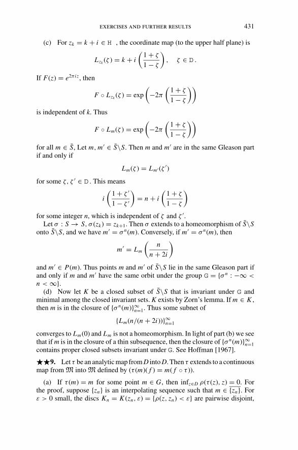
exercises and further results 431
(c) For zk = k + i ∈ H , the coordinate map (to the upper half plane) is
Lzk (ζ ) = k + i
(1 + ζ
1 − ζ
)
, ζ ∈ D .
If F(z) = e2π i z , then
F ◦ Lzk (ζ ) = exp
(
−2π
(1 + ζ
1 − ζ
))
is independent of k. Thus
F ◦ Lm(ζ ) = exp
(
−2π
(1 + ζ
1 − ζ
))
for all m ∈ S, Let m, m ′ ∈ S\S. Then m and m ′ are in the same Gleason partif and only if
Lm(ζ ) = Lm ′(ζ ′)
for some ζ, ζ ′ ∈ D . This means
i
(1 + ζ ′
1 − ζ ′
)
= n + i
(1 + ζ
1 − ζ
)
for some integer n, which is independent of ζ and ζ ′.Let σ : S → S, σ (zk) = zk+1. Then σ extends to a homeomorphism of S\S
onto S\S, and we have m ′ = σ n(m). Conversely, if m ′ = σ n(m), then
m ′ = Lm
(n
n + 2i
)
and m ′ ∈ P(m). Thus points m and m ′ of S\S lie in the same Gleason part ifand only if m and m ′ have the same orbit under the group G = {σ n : −∞ <
n < ∞}.(d) Now let K be a closed subset of S\S that is invariant under G and
minimal among the closed invariant sets. K exists by Zorn’s lemma. If m ∈ K ,then m is in the closure of {σ n(m)}∞n=1. Thus some subnet of
{Lm(n/(n + 2i))}∞n=1
converges to Lm(0) and Lm is not a homeomorphism. In light of part (b) we seethat if m is in the closure of a thin subsequence, then the closure of {σ n(m)}∞n=1
contains proper closed subsets invariant under G. See Hoffman [1967].
��9. Let τ be an analytic map from D into D. Then τ extends to a continuousmap from M into M defined by (τ (m)( f ) = m( f ◦ τ )).
(a) If τ (m) = m for some point m ∈ G, then infz∈D ρ(τ (z), z) = 0. Forthe proof, suppose {zn} is an interpolating sequence such that m ∈ {zn}. Forε > 0 small, the discs Kn = K (zn, ε) = {ρ(z, zn) < ε} are pairwise disjoint,

432 interpolating sequences and maximal ideals Chap. X
and m is not in the closure of D\ ⋃∞n=1 Kn . Consequently the relation f (zn) ∈
k j holds for infinitely many n, say for n ∈ S. Write T (n) = j when n ∈ Sand f (zn) ∈ K j . The problem is to show that T has a fixed point. Definean equivalence relation in S by setting n1 ∼ n2 if T p(n1) = T q (n2) for somenonnegative integers p and q. Note that n ∼ T (n) if n ∈ S and if T (n) ∈ S. Letn∗ denote the least element of the equivalence class containing n. Let E be theset of n ∈ S such that p + q is even, where p + q is the smallest such integersuch that T p(n) = T q (n∗). If T has no fixed point in S, then when n ∈ S andT (n) ∈ S, exactly one of n and T (n) lies in E.
Let B(z) be the Blaschke product with zeros on S. Then B(m) = 0. FactorB = B1 B2, where B1 has zeros {zn : n ∈ E} and B2 has zeros {zn : n ∈ S\E}.When ε is small, the assumption that T has no fixed point now leads to acontradiction.
(b) If τ has two fixed points in G lying in different fibers, then τ (z) = z.(Use part (b) and Exercise 2 of Chapter I.)
(c) Let Mλ be the fiber of M at λ, |λ| = 1. Then τ fixed a point in G ∩ Mλ
if and only if the angular derivative of τ exists at λ and equals 1 there. (SeeExercise 7 of Chapter I for a discussion of angular derivatives.)
(d) τ maps the Silov boundary into itself if and only if τ (z) is an innerfunction.
(These results are due to Michael Behrens.)
10. Let m ∈ M and let f ∈ H∞, f (m) = 0. Then
limz→m
| f ′(z)|(1 − |z|2) = 0
if and only if f = f1 f2 with f j ∈ H∞, f j (m) = 0. (The only interesting caseis that in which f (z) is a Blaschke product, because both conditions holdtrivially if f 1/2 ∈ H∞. When m /∈ G, both conditions follow from Theorem2.4. When m ∈ G, each condition means that ( f ◦ Lm)′(0) = 0.)
11. Let B0 be the class of analytic functions on D satisfying
lim|z|→1
(1 − |z|2)| f ′(z)| = 0,
and let VMOA be the analytic functions of the form u + v, u, v harmonic onD and continuous on D. Here B stands for Bloch.
(a) VMOA ⊂ B0.(b) f (z) ∈ H∞ ∩ B0 if and only if f (m) is constant on each Gleason part
in M\D. For this reason Behrens called this class COP, for constant on parts.(c) Suppose g(z) is in the disc algebra. Then g(eiθ ) is in the Zygmund class
�∗, defined by
|g(θ + h) − g(θ − h) − 2g(θ )| = O(h)
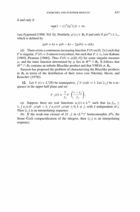
exercises and further results 433
if and only if
supz
(1 − |z|2)|g′′(z)| < ∞.
(see Zygmund [1968, Vol. I]). Similarly, g′(z) ∈ B0 if and only if g(eiθ ) ∈ λ∗,which is defined by
|g(θ + h) + g(θ − h) − 2g(θ )| = o(h).
(d) There exists a continuous increasing function F(θ ) on [0, 2π ] such thatF is singular, F ′(θ ) = 0 almost everywhere, but such that F ∈ λ∗ (see Kahane[1969], Piranian [1966]). Thus F(θ ) = μ([0, θ ]) for some singular measureμ, and the inner function determined by μ lies in H∞ ∩ B0. It follows thatH∞ ∩ B0 contains an infinite Blaschke product and that VMOA = B0.
Sarason has proposed the problem of characterizing the Blaschke productsin B0 in terms of the distribution of their zeros (see Nikolski, Havin, andKruschev [1978]).
12. Let P (t) ∈ L1(�) be nonnegative,∫P (t)dt = 1. Let {z j } be a se-
quence in the upper half plane and set
P j (t) = 1
y jP
(t − x j
y j
)
.
(a) Suppose there are real functions u j (t) ∈ L∞ such that ‖u j‖∞ ≤1,
∫u j (t)P j (t)dt > δ,
∫u j (t)P k(t)dt ≤ 0, k = j , with δ independent of j.
Then {z j } is an interpolating sequence.(b) If the weak-star closure of {P j } in (L∞)∗ homeomorphic β�, the
Stone–Cech compactification of the integers, then {z j } is an interpolatingsequence.

Bibliography
Adamyan, V. M., Arov, D. Z., and Krein, M. G.
[1968] Infinite Hankel matrices and generalized problems of Caratheodory, Fejer
and I. Schur, Funkcional Anal. i Prilozen. 2, vyp 4, 1–17 (Russian); FunctionalAnal. Appl. 2, 269–281.
[1971] Infinite Hankel block matrices and related approximation problems, VestnikAkad. Nauk Armjan. SSR 6, 87–102 (Russian); Amer. Math. Soc. Transl. (2) 111(1978), 133–156.
Ahern, P. R., and Clark, D. N.
[1970a] On functions orthogonal to invariant subspaces, Acta Math. 124, 191–204.
[1970b] Radial limits and invariant subspaces, Amer. J. Math. 92, 332–342.
[1971] Radial Nth derivatives of Blaschke products, Math. Scand. 28, 189–201.
[1974] On inner functions with H p derivatives, Michigan Math. J. 21, 115–127.
[1976] On inner functions with B p derivatives, Michigan Math. J. 23, 107–118.
Ahlfors, L. V.
[1966] “Complex Analysis” (2nd ed.). McGraw-Hill, New York.
[1973] “Conformal Invariants, Topics in Geometric Function Theory.” McGraw-Hill,
New York.
Alexander, H., Taylor, B. A., and Williams, D. L.
[1971] The interpolating sets for A∞, J. Math. Anal. Appl. 36, 556–566.
Allen, H. A., and Belna, C. L.
[1972] Singular inner functions with derivatives in B p , Michigan Math. J. 19, 185–
188.
Amar, E.
[1973] Sur un theoreme de Mooney relatif aux fonctions analytiques bornees, PacificJ. Math. 16, 191–199.
[1977a] These, Faculte des Sciences d’Orsay, Universite de Paris XI.
[1977b] Suites d’interpolation harmoniques, J. Analyse Math. 32, 197–211.
Amar, E., and Lederer, A.
[1971] Points exposes de la boule unite de H∞(D), C. R. Acad. Sci. Paris. Ser. A272, 1449–1552.
Anderson, J. M.
[1975] A note on a basis problem, Proc. Amer. Math. Soc. 51, 330–334.
[1979] On division by inner factors, Comment. Math. Helv. 54, 309–317.
434

bibliography 435
Anderson, J. M., Clunie, J., and Pommerenke, Ch.
[1974] On Bloch functions and normal functions, J. Reine Angew. Math. 270, 12–37.
Ando, T.
[1977] Uniqueness of predual of H∞, preprint.
Axler, S.
[1977] Factorization of L∞ functions, Ann. of Math. 106, 567–572.
Axler, S., Berg, I. D., Jewell, N. P., and Shields, A.
[1979] Approximation by compact operators and the space H∞ + C , Ann. of Math.
109, 601–612.
Axler, S., Chang, S.-Y., and Sarason, D.
[1978] Products of Toeplitz operators, Integral Equations Operator Theory 1/3, 285–
309.
Baernstein, A.
[1974] Integral means, univalent functions and circular symmetrization, Acta Math.133, 139–169.
[1976] Univalence and bounded mean oscillation, Michigan Math. J. 23, 217–223.
[1979] Some sharp inequalities for conjugate functions, Proc. Symp. Pure Math. 35(1), 409–416.
[1980] Analytic functions of bounded mean oscillation in “Aspects of Contemporary
Complex Analysis. Academic Press, New York.
Bagemihl, F., and Seidel, W.
[1954] Some boundary properties of analytic functions, Math. Z. 61, 186–189.
Barbey, K.
[1975] Ein Satz uber abstrakte analytische Funktionen, Arch. Math. (Basel) 26, 521–
527.
Bear, H. S.
[1970] “Lecture on Gleason Parts” (Lecture Notes in Mathematics, Vol. 121).
Springer-Verlag, Berlin and New York.
Behrens, M.
[1971] The maximal ideal space of algebras of bounded analytic functions on in-
finitely connected domains, Trans. Amer. Math. Soc. 161, 358–380.
[1981] Interpolation and Gleason parts in L-domains, Trans. Amer. Math. Soc. 286(1984), 203–225.
Belna, C., and Piranian, C.
[1981] A Blaschke product with a level-set of infinite length, to be published.
Bernard, A.
[1971] Algebres quotients d’algebres uniformes, C. R. Acad. Sci. Paris, Ser. A 272,
1101–1104.
Bernard, A., Garnett, J. B., and Marshall, D. E.
[1977] Algebras generated by inner functions, J. Funct. Anal. 25, 275–285.
Besicovitch, A.
[1923] Sur la nature des fonctions a carre sommable measurables, Fund. Math. 4,
172–195.
Bessaga, C., and Pelczynski, A.
[1960] Spaces of continuous functions (IV), Studia Math. 19, 53–62.

436 bibliography
Beurling, A.
[1949] On two problems concerning linear transformations in Hilbert space, ActaMath. 81, 239–255.
Bishop, E.
[1959] A minimal boundary for function algebras, Pacific J. Math. 9, 629–642.
[1962] A general Rudin–Carleson theorem, Proc. Amer. Math. Soc. 13, 140–
143.
[1963] Holomorphic completions, analytic continuations, and the interpolation of
seminorms, Ann. of Math. 78, 468–500.
[1964] Representing measures for points in a uniform algebra, Bull. Amer. Math.Soc. 70, 121–122.
[1965] Abstract dual extremal problems, Notices Amer. Math. Soc. 12, 123.
Bishop, E., and Phelps, R. R.
[1961] A proof that every Banach space is subreflexive, Bull. Amer. Math. Soc. 67,
97–98.
Blaschke, W.
[1915] Eine Erweiterung des Satzes von Vitali uber Folgen analytischer Funktionen,
S.-B. Sacks Akad. Wiss. Leipzig Math.-Natur. KI. 67, 194–200.
Bockarev, V.
[1974] Existence of a basis in the space of analytic functions, and some properties
of the Franklin system. Math. USSR-Sb. 24, 1–16.
Boyd, D.
[1979] Schur’s algorithm for bounded holomorphic functions, Bull. London Math.Soc. 11, 145–150.
Browder, A.
[1969] “Introduction to Function Algebras.” Benjamin, New York.
Brown, L.
[1970] Subalgebras of L∞ of the circle group, Proc. Amer. Math. Soc. 25, 585–587.
Brown, L., Shields, A., and Zeller, K.
[1960] On absolutely convergent exponential sums, Trans. Amer. Math. Soc. 96,
162–183.
Burkholder, D. L.
[1973] Distribution function inequalities for martingales, Ann. Probability 1, 19–42.
[1976] Harmonic analysis and probability, in “Studies in Harmonic Analysis” (J. M.
Ash, ed.), Studies in Math. Vol. 13, 13, pp 136–149.
[1979] Martingale theory and harmonic analysis in Euclidean spaces, Proc. Symposiain Pure Math. 35 (2), 283–302.
Burkholder, D. L., and Gundy, R. F.
[1972] Distribution function inequalities for the area integral, Studia Math. 44, 527–
544.
Burkholder, D. L., Gundy, R. F., and Silverstein, M. L.
[1971] A maximal function characterization of the class H p , Trans. Amer. Math.Soc. 157, 137–153.
Calderon, A. P.
[1950a] On theorems of M. Riesz and Zygmund, Proc. Amer. Math. Soc. 1, 533–535.
bibliography 437
[1950b] On the behavior of harmonic functions near the boundary, Trans. Amer.Math. Soc. 68, 47–54.
Calderon, A. P., and Zygmund, A.
[1952] On the existence of certain singular integrals, Acta Math. 88, 85–139.
[1956] On singular integrals, Amer. J. Math. 78, 249–271.
Campanato, S.
[1963] Propreita de holderianita di alcane classi di funzioni, Ann. Scuola Norm. Sup.Pisa (3) 17, 175–188.
Cantor, D. G.
[1981] Oral communication.
Caratheodory, C.
[1911] Uber den Variabilitatsbereich der Fourier’schen Konstanten von positiven
harmonischen Funktionen, Rend. Circ. Mat. Palermo 32, 193–217.
[1929] Uber die Winkelderivierten von beschrankten analytischen Funktionen,
Sitzungsber Preuss. Akad. Phys.-Math. 4, 1–18.
[1954] “Theory of Functions of a Complex Variable,” Vols. I and II. Chelsea, New
York.
Cargo, G. T.
[1962] Angular and tangential limits of Blaschke products and their successive
derivatives, Canad. J. Math. 14, 334–348.
Carleson, L.
[1952] Sets of uniqueness for functions analytic in the unit disc, Acta. Math. 87,
325–345.
[1957] Representations of continuous functions, Math. Z. 66, 447–451.
[1958] An interpolation problem for bounded analytic functions, Amer. J. Math. 80,
921–930.
[1962a] Interpolations by bounded analytic functions and the corona problem, Ann.of Math. 76, 547–559.
[1962b] Interpolations by bounded analytic functions and the corona problem, Proc.Internat. Congr. Math. Stockholm. 314–316.
[1967] “Selected Problems on Exceptional Sets.” Van Nostrand-Reinhold, Princeton,
New Jersey.
[1970] The corona theorem, Proc. Scand. Congr., 15th, Oslo (Lecture Notes in Math-
ematics, Vol. 118). Springer-Verlag, Berlin and New York.
[1972] A moment problem and harmonic interpolation, preprint, Inst. Mittag-Leffler,
Djursholm.
[1976] Two remarks on H 1 and BMO, Advances in Math, 22, 269–277.
Carleson, L., and Garnett, J.
[1975] Interpolating sequences and separation properties, J. Analyse Math. 28, 273–
299.
Carleson, L., and Jacobs, S.
[1972] Best approximation by analytic functions, Ark. Mat. 10, 219–229.
Caughran, J. G., and Shields, A. L.
[1969] Singular inner factors of analytic functions, Michigan Math. J. 16 (1969),
409–410.
438 bibliography
Chang, S.-Y.
[1976] A characterization of Douglas subalgebras, Acta Math. 137, 81–89.
[1977a] Structure of subalgebras between L∞ and H∞, Trans. Amer. Math. Soc. 227,
319–332.
[1977b] On the structure and characterization of some Douglas subalgebras, Amer.J. Math. 99, 530–578.
Chang, S.-Y., and Garnett, J. B.
[1978] Analytically of functions and subalgebras of L∞ containing H∞, Proc. Amer.Math. Soc. 72, 41–46.
Chang, S.-Y., and Marshall, D. E.
[1977] Some algebras of bounded analytic functions containing the disc algebra,
“Banach Spaces of Analytic Functions” (Lecture Notes in Math., Vol. 604, pp. 12–
20). Springer-Verlag, Berlin and New York.
Chaumat, J.
[1978] Quelques proprietes du couple d’espace vectoriels (L1(m)/H∞ ⊥,
H∞), preprint. Univ. de Paris-Sud, Orsay.
Cima, J. A., and Petersen, K. E.
[1976] Some analytic functions whose boundary values have bounded mean oscil-
lation, Math. Z. 147, 237–247.
Cima, J. A., and Schober, G.
[1976] Analytic functions with bounded mean oscillation and logarithms of H p-
functions, Math. Z. 151, 295–300.
Clark, D. N.
[1968a] Hankel forms, Toeplitz forms and meromorphic functions, Trans. Amer.Math. Soc. 134, 109–116.
[1968b] On the spectra of bounded, hermitian, Hankel matrices, Amer. J. Math. 90,
627–656.
[1968c] On matrices associated with generalized interpolation problems,
Pacific J. Math. 27, 241–253.
[1970] On interpolating sequences and the theory of Hankel and Toeplitz matrices,
J. Func. Anal. 5, 247–258.
Cohen, P. J.
[1961] A note on constructive methods in Banach algebras, Proc. Amer. Math. Soc.12, 159–163.
Coifman, R. R.
[1974] A real variable characterization of H p , Studia Math. 51, 269–274.
Coifman, R. R., and Fefferman, C.
[1974] Weighted norm inequalities for maximal functions and singular integrals,
Studia Math. 51, 241–250.
Coifman, R. R., and Meyer, Y.
[1975] On commutators of singular integrals and bilinear singular integrals, Trans.Amer. Math. Soc. 212, 315–331.
Coifman, R. R., and Rochberg, R.
[1980] Another characterization of BMO, Proc. Amer. Math. Soc. 79, 249–254.
Coifman, R. R., Rochberg, R., and Weiss, G.
bibliography 439
[1976] Factorization theorems for Hardy spaces in several complex variables, Ann.of Math. 103, 611–635.
Coifman, R. R., and Weiss, G.
[1971] “Analysis harmonique non-commutative sur certains espaces homogenes”
(Lecture Notes in Mathematics, Vol. 242). Springer-Verlag, Berlin and New
York.
[1977] Extensions of Hardy spaces and their uses in analysis, Bull. Amer. Math. Soc.83, 569–646.
Collingwood, E. F., and Lohwater, A. J.
[1966] “The Theory of Cluster Sets.” Cambridge Univ. Press, London and New York.
Cordoba, A., and Fefferman, C.
[1976] A weighted norm inequality for singular integrals, Studia Math. 57, 97–
101.
Dahlberg, B. J. E.
[1980] Approximation of harmonic functions, Ann. Inst. Fourier (Grenoble) 30, 2,
97–107.
Davie, A. M.
[1972] Linear extension operators for spaces and algebras of functions, Amer. J.Math. 94, 156–172.
Davie, A. M., Gamelin, T. W., and Garnett, J. B.
[1973] Distance estimates and pointwise bounded density, Trans. Amer. Math. Soc.175, 37–68.
Davis, B. J.
[1974] On the weak type (1, 1) inequality for conjugate functions, Proc. Amer. Math.Soc. 44, 307–311.
[1976] On Kolmogorov’s inequalities || f ||p ≤ cp|| f ||1, 0 < p < 1, Trans. Amer.Math. Soc. 222, 179–192.
Dawson, D. W.
[1975] Subalgebras of H∞, Thesis, Indiana Univ., Bloomington, Indiana.
deLeeuw, K., and Rudin, W.
[1958] Extreme points and extreme problems in H1, Pacific J. Math. 8, 467–485.
Denjoy, A.
[1929] Sur une classe de fonctions analytiques, C.R. Acad. Sci. Paris, Ser. A.-B 188,
140, 1084.
Diximier, J.
[1951] Sur certains espaces consideres par M. H. Stone, Summa Brasil Math. 2,
151–182.
Donoghue, W. F.
[1974] “Monotone Matrix Functions and Analytic Continuation.” Springer-Verlag,
Berlin and New York.
Douglas, R. G.
[1969] On the spectrum of Toeplitz and Wiener–Hopf operators, in “Abstract Spaces
and Approximation Theory,” pp. 53–66. Birkhauser, Basel.
[1972] “Banach Algebra Techniques in Operator Theory.” Academic Press, New
York.

440 bibliography
Douglas, R. G., and Rudin, W.
[1969] Approximation by inner functions, Pacific J. Math. 31, 313–320.
Douglas, R. G., Shapiro, H. S., and Shields, A. L.
[1970] Cyclic vectors and invariant subspaces for the backward shift operator, Ann.Inst. Fourier (Grenoble) 20, 1, 37–76.
Drury, S.
[1970] Sur les ensembles de Sidon, C.R. Acad. Sci. Paris, Ser. A, 271, 162–163.
Dunford, N., and Schwartz, J.
[1958] “Linear Operators,” Part I, Wiley (Interscience), New York.
Duren, P. L.
[1970] “Theory of H p Spaces.” Academic Press, New York.
Duren, P. L., Romberg, B. W., and Shields, A. L.
[1969] Linear functionals on H p spaces with 0 < p < 1, J. Reine Angew. Math. 238,
32–60.
Duren, P. L., Shapiro, H. S., and Shields, A. L.
[1966] Singular measures and domains not of Smirnov type, Duke Math. J. 33, 247–
254.
Dym, H., and McKean, H. P.
[1976] “Gaussian Processes, Function Theory, and the Inverse Spectral Problem.”
Academic Press, New York.
Earl, J. P.
[1970] On the interpolation of bounded sequences by bounded functions, J. LondonMath. Soc. (2) 2, 544–548.
[1976] A note on bounded interpolation in the unit disc, J. London Math. Soc. (2)
13, 419–423.
Fatou, P.
[1906] Series trigonometriques et series de Taylor, Acta Math. 30, 335–400.
Fefferman, C.
[1971] Characterizations of bounded mean oscillation, Bull. Amer. Math. Soc. 77,
587–588.
[1974] Harmonic analysis and H p spaces, in “Studies in Harmonic Analysis” (J. M.
Ash, ed.), Studies in Math. Vol. 13, pp. 38–75.
Fefferman, C., and Stein, E. M.
[1972] H p spaces of several variables, Acta Math. 129, 137–193.
Fisher, S.
[1968] The convex hull of the finite Blaschke products, Bull. Amer. Math. Soc. 74,
1128–1129.
[1969a] Another theorem on convex combinations of unimodular functions, Bull.Amer. Math, Soc. 75, 1037–1039.
[1969b] Exposed points in spaces of bounded analytic functions, Duke Math. J. 36,
479–484.
[1971] Approximation by unimodular functions, Canad. J. Math. 23, 257–269.
Forelli, F.
[1963a] The Marcel Riesz theorem on conjugate functions, Trans. Amer. Math. Soc.106, 369–390.

bibliography 441
[1963b] Analytic measures, Pacific J. Math. 13, 571–578.
[1964] The isometries of H P , Can. J. Math. 16, 721–728.
Fournier, J.
[1974] An interpolation problem for coefficients of H∞ functions, Proc. Amer. Math.Soc. 42, 402–408.
Frostman, O.
[1935] Potential d’equilibre et capacite des ensembles avec quelques applications a
la theorie des fonctions. Medd. Lunds Univ. Mat. Sem. 3, 1–118.
Gamelin, T. W.
[1964] Restrictions of subspaces of C(X ), Trans. Amer. Math. Soc. 112, 278–286.
[1969] “Uniform Algebras.” Prentice Hall, Englewood Cliffs, New Jersey.
[1970] Localization of the corona problem, Pacific J. Math. 34, 73–81.
[1972] “Lectures on H∞(D).” Univ. Nacional de la Plata, Argentine.
[1973] Extremal problems in arbitrary domains, Michigan Math. J. 20, 3–11.
[1974] The Silov boundary of H∞(U ), Amer. J. Math. 94, 79–103.
[1979] “Uniform Algebras and Jensen Measures.” London Math. Society Lecture
Notes Series, 32. Cambridge Univ. Press, London and New York.
[1981] Wolff’s proof of the corona theorem, Israel J. Math., in press.
Gamelin, T. W., and Garnett, J.
[1970] Distinguished homomorphisms and fiber algebras, Amer. J. Math. 92, 455–
474.
Gamelin, T. W., Garnett, J. B., Rubel, L. A., and Shields, A. L.
[1976] On badly approximable functions, J. Approx. Theory 17, 280–296.
Garnett, J.
[1971a] Vitushkin’s localization operator, Indiana Univ. Math. J. 20, 905–907.
[1971b] Interpolating sequences for bounded harmonic functions, Indiana Univ.Math. J. 21, 187–192.
[1977] Two remarks on interpolation by bounded analytic functions, “Banach Spaces
of Analytic Functions” (Baker et al., eds.) (Lecture Notes in Math. Vol. 604).
Springer-Verlag, Berlin.
[1978] Harmonic interpolating sequences, L p and BMO, Ann. Inst. Fourier (Greno-ble) 28, 215–228.
Garnett, J. B., and Jones, P. W.
[1978] The distance in BMO to L∞, Ann. of Math. 108, 373–393.
Garnett, J. B., and Latter, R. H.
[1978] The atomic decomposition for Hardy spaces in several complex variables,
Duke Math. J. 45, 815–845.
Garsia, A.
[1970] “Topics in Almost Everywhere Convergence.” Markham, Chicago, Illinois.
[1971] A presentation of Fefferman’s theorem, unpublished notes.
[1973] “Martingale Inequalities.” Benjamin, New York.
Gehring, F. W.
[1973] The L p-integrability of the partial derivatives of a quasiconformal mapping,
Acta Math. 130, 265–277.
Glicksberg, I.

442 bibliography
[1962] Measures orthogonal to algebras and sets of antisymmetry, Trans. Amer. Math.Soc. 105, 415–435.
[1967] The abstract F. Riesz and M. Riesz Theorem, J. Funct. Anal. 1, 109–122.
Goluzin, G. M.
[1952] “Geometric Theory of Functions of a Complex Variable, Moscow, 1952, (in
Russian) [English Transl.: Amer. Math. Soc., Providence, Rhode Island, 1969].
Grenander, U., and Rosenblatt, M.
[1957] “Statistical Analysis of Stationary Time Series.” Wiley, New York.
Grothendieck, A.
[1955] Une caracterization vectoriellemetrique des espaces L1, Canad. J. Math. 7,
552–561.
Gundy, R. F., and Wheeden, R. L.
[1974] Weighted integral inequalities for the non-tangential maximal function, Lusin
area integral, and Walsh–Paley series, Studia Math. 49, 107–124.
Hall, T.
[1937] Sur la mesure harmonique de certains ensembles, Ark. Mat. Astr. Fys. 25A,
No. 28.
Hardy, G. H., and Littlewood, J. E.
[1927] Some new properties of Fourier constants, Math. Ann. 97, 159–209.
[1930] A maximal theorem with function-theoretic applications, Acta Math. 54, 81–
116.
[1932] Some properties of conjugate functions, J. Reine Angew. Math. 167, 405–423.
[1936] Some more theorems concerning Fourier series and Fourier power series,
Duke Math. J. 2, 354–382.
Hartman, P.
[1958] On completely continuous Hankel matrices, Proc. Amer. Math. Soc. 9, 862–
866.
Havin, V. P.
[1973] Weak completeness of the space L1/H 10 , Vestnik Leningrad Univ. 13, 77–81
(in Russian).
[1974] The spaces H∞ and L1/H 10 , Issl. po Lin. Operat. Tieor. Funk. IV, Zap. Naucn
Sem. Leningrad. Otdel. Mat. Inst. Steklov (LOMI) 29, 120–148 (in Russian).
Havin, V. P., and Vinogradov, S. A.
[1974] Free interpolation in H∞ and some other function classes, 1, Zap. Naucn.Sem. Leningrad. Otdel. Mat. Inst. Steklov (LOMI ) 47, 15–54 (in Russian).
Havinson, S. Ja.
[1949] On an extremal problem in the theory of analytic functions, Usp. Mat. Nauk.4, No. 4 (32), 158–159 (in Russian).
[1951] On some external problems in the theory of analytic functions, Moskov. Gos.Univ. Ucen. Zap. 148, Matem. 4, 133–143 (in Russian); Amer. Math. Soc. Transl.(2) 32, 139–154.
Hayman, W. K.
[1974] On a theorem of Tord Hall, Duke Math. J. 41, 25–26.
Hayman, W. K., and Kennedy, P. L.
[1976] “Subharmonic Functions.” Academic Press, New York.

bibliography 443
Hayman, W. K., and Pommerenke, Ch.
[1978] On analytic functions of bounded mean oscillation, Bull. London Math. Soc10, 219–224.
Heard, E. A., and Wells, J. H.
[1969] An interpolation problem for subalgebras of H∞, Pacific J. Math. 28, 543–
553.
Helson, H.
[1964] “Lectures on Invariant Subspaces.” Academic Press, New York.
Helson, H., and Sarason, D.
[1967] Past and future, Math. Scand. 21, 5–16.
Helson, H., and Szego, G.
[1960] A problem in prediction theory, Ann. Mat. Pura Appl. 51, 107–138.
Hormander, L.
[1966] “An Introduction to Complex Analysis in Several Variables.” Van Nostrand-
Reinhold, Princeton, New Jersey.
[1967a] Generators for some rings of analytic functions, Bull. Amer. Math. Soc. 73,
943–949.
[1967b] L p estimates for (pluri-) subharmonic functions, Math. Scand. 20, 65–
78.
Hoffman, K.
[1962a] “Banach Spaces of Analytic Functions.” Prentice Hall, Englewood Cliffs,
New Jersey.
[1962b] Analytic functions and logmodular Banach algebras, Acta Math. 108, 271–
317.
[1967] Bounded analytic functions and Gleason parts, Ann. of Math. 86, 74–
111.
Hoffman, K., and Ramsey, A.
[1965] Algebras of bounded sequences, Pacific J. Math. 5, 1239–1248.
Hoffman, K., and Rossi, H.
[1967] Extensions of positive weak∗-continuous functionals, Duke Math. J. 34, 453–
466.
Hoffman, K., and Singer, I. M.
[1957] Maximal subalgebras of C(�), Amer. J. Math. 79, 295–305.
[1960] Maximal algebras of continuous functions, Acta Math. 103, 217–241.
Hunt, R. A., Muckenhoupt, B., and Wheeden, R. L.
[1973] Weighted norm inequalities for the conjugate function and Hilbert transform,
Trans. Amer. Math. Soc. 176, 227–251.
Jensen, J. L. W. V.
[1899] Sur un nouvel et important theoreme de la theorie des fonctions, Acta Math.22, 219–251.
[1906] Sur les fonctions convexes et les inegalites entre les valeurs moyennes, ActaMath. 30, 175–193.
Jerison, D.
[1976] Sur un theoreme d’interpolation de R. Nevanlinna, C.R. Acad. Sci. Paris, Ser.A 282, 1291–1293.

444 bibliography
Jewell, N.
[1976] Continuity of Derivations and Uniform Algebras on Odd Spheres. Thesis,
Univ. of Edinburgh.
John, F., and Nirenberg, L.
[1961] On functions of bounded mean oscillation, Comm. Pure Appl. Math. 14,
415–426.
Jones, P.
[1979a] A complete bounded complex submanifold of C3, Proc. Amer. Math. Soc.76, 305–306.
[1979b] Constructions for BMO (�n) and Ap(�n), Proc. Symposia in Pure Math. 35(1), 409–416.
[1979c] Extension theorems for BMO, Indiana Univ. Math. J. 29, 41–
66.
[1980a] Bounded holomorphic functions with all level sets of infinite length, Michi-gan Math. J. 27, 75–79.
[1980b] Carleson measures and the Fefferman–Stein decomposition of BMO(�),
Ann. of Math. 111, 197–208.
[1980c] Factorization of Ap weights, Ann. of Math. 111, 511–530.
[1980d] Estimates for the corona problem, J. Funct. Anal. 39, 162–181.
[1981] Ratios of interpolating Blaschke products, Pacific J. Math., in press.
Julia, G.
[1920] Extension d’un lemma de Schwarz, Acta Math. 42, 349–355.
Kahane, J. P.
[1967] Another theorem on bounded analytic functions, Proc. Amer. Math. Soc. 18,
818–826.
[1969] Trois notes sur les ensembles parfaits lineaires, Enseignement Math. 15, 185–
192.
[1974] Best approximation in L1(T ), Bull. Amer. Math. Soc. 80, 788–804.
Katznelson, Y.
[1968] “An Introduction to Harmonic Analysis.” Wiley, New York.
Kelleher, J. J., and Taylor, B. A.
[1971] Finitely generated ideals in rings of analytic functions, Math. Ann. 193, 225–
237.
Kelley, J. L.
[1955] “General Topology.” Van Nostrand-Reinhold, Princeton, New Jersey.
Kerr-Lawson, A.
[1965] A filter description of the homomorphisms of H∞, Canad. J. Math. 17, 734–
757.
[1969] Some lemmas on interpolating Blaschke products and a correction, Canad.J. Math. 21, 531–534.
Konig, H.
[1969] On the Gleason and Harnack metrics for uniform algebras, Proc. Amer. Math.Soc. 22, 100–101.
Kolmogoroff, A. N.
[1925] Sur les fonctions harmoniques conjuquees et les series de Fourier, Fund.Math. 7, 24–29.

bibliography 445
[1941] Stationary sequences in Hilbert space, Bull. Math. Univ. Moscow 2, No. 6 (in
Russian).
Koosis, P.
[1971] Weighted quadratic means of Hilbert transforms, Duke Math. J. 38, 609–
634.
[1973] Moyennes quadratiques de transformees de Hilbert et fonctions de type ex-
ponential, C.R. Acad. Sci. Paris, Ser. A 276, 1201–1204.
[1978] Sommabilite de la fonction maximale et appartenance a H1, C.R. Acad. Sci.Paris, Ser. A 286, 1041–1043.
[1979] Sommabilite de la fonction maximale et appartenance a H1, Cas de plusieurs
variables, C.R. Acad. Sci. Paris, Ser. A 288, 489–492.
[1980] “Lectures on Hp Spaces,” London Math. Society Lecture Notes Series, 40.
Cambridge Univ. Press, London and New York.
Landau, E.
[1913] Abschatzung der Koeffizientensumme einer Potenzreihe, Arch. Math. Phys.21, 42–50, 250–255.
[1916] “Darstellung und Begrundung einiger neuerer Ergebnisse der Funktionenthe-
orie.” Berlin; [1946] reprinted by Chelsea, New York.
Latter, R. H.
[1978] A decomposition of H p(�n) in terms of atoms, Studia Math. 62, 92–
101.
Lindelof, E.
[1915] Sur un principle generale de l’analyse et ces applications a la theorie de la
representation conforme, Acta Soc. Sci. Fenn. 46, No. 4.
Littlewood, J. E.
[1929] On functions subharmonic in a circle, II. Proc. London Math. Soc. 28, 383–
394.
Littlewood, J. E., and Paley, R. E. A. C.
[1931] Theorems on Fourier series and power series, (I), J. London Math. Soc. 6,
230–233; (II) ibid. 42, 52–89; (III) ibid. 43, 105–126.
Loomis, L. H.
[1946] A note on the Hilbert transform, Bull. Amer. Math. Soc. 52, 1082–1086.
Luecking, D.
[1980] The compact Hankel operators form an M-ideal in the space of Hankel oper-
ators, Proc. Amer. Math. Soc. 79, 222–224.
Lumer, G.
[1965] Analytic functions and the Dirichlet problem, Bull. Amer. Math. Soc. 70,
98–104.
[1969] “Algebres de fonctions et espaces de Hardy” (Lecture Notes in Math., Vol.
75). Springer-Verlag, Berlin and New York.
Macintyre, A. J., and Rogosinski, W. W.
[1950] Extremum problems in the theory of analytic functions, Acta Math. 82, 275–
325.
Marden, M.
[1966] Geometry of polynomials, Amer. Math. Soc. Math. Surveys, No. 3, 2nd ed.
446 bibliography
Marshall, D. E.
[1974] An elementary proof of the Pick–Nevanlinna interpolation theorem, MichiganMath. J. 21, 219–233.
[1976a] Blaschke products generate H∞, Bull. Amer. Math. Soc. 82, 494–
496.
[1976b] Subalgebras of L∞ containing H∞, Acta Math. 137, 91–98.
[1976c] Approximation and interpolation by inner functions. Thesis, Univ. of Cali-
fornia, Los Angeles, California.
Meyers, N. G.
[1964] Mean oscillation over cubes and Holder continuity, Proc. Amer. Math. Soc.15, 717–721.
Mooney, M. C.
[1973] A theorem on bounded analytic functions, Pacific J. Math. 43, 457–463.
Muckenhoupt, B.
[1972] Weighted norm inequalities for the Hardy maximal function, Trans. Amer.Math. Soc. 165, 207–226.
[1974] The equivalence of two conditions for weighted functions, Studia Math. 49,
101–106.
[1979] Weighted norm inequalities for classical operators, Proc. Symposia in PureMath. 35 (1), 69–84.
Muckenhoupt, B., and Wheeden, R. L.
[1974] Weighted norm inequalities for fractional integrals, Trans. Amer. Math. Soc.192, 261–274.
Natzitz, B.
[1970] A note on interpolation, Proc. Amer. Math. Soc. 25, 918.
Negrepontis, S.
[1967] On a theorem of Hoffman and Ramsey, Pacific J. Math. 20, 281–282.
Neri, U.
[1977] Some properties of functions with bounded mean oscillation, Studia Math.61, 63–75.
Neuwirth, J., and Newman, D. J.
[1967] Positive H 1/2 functions are constant, Proc. Amer. Math. Soc. 18, 958.
Nevanlinna, F., and Nevanlinna, R.
[1922] Eigenschaften analyscher Funktionen in der Umgebung einer singularen
Stelle oder Linie, Acta Soc. Sci. Fenn. 50, No. 5.
Nevanlinna, R.
[1919] Uber beschrankte Funktionen, die in gegebenen Punkten vorgeschrieben
Werte annehmen, Ann. Acad. Sci. Fenn. Ser. A, 13, No. 1.
[1929] Uber beschrankte analytische Funktionen, Ann. Acad. Sci. Fenn. 32,
No. 7.
[1953] “Eindeutige analytische Funktionen,” Vol. 2, Auflage. Springer-Verlag, Berlin
and New York.
Newman, D. J.
[1959a] Interpolation in H∞, Trans. Amer. Math. Soc. 92, 501–507.
[1959b] Some remarks on the maximal ideal space structure of H∞, Ann. of Math.70, 438–445.
bibliography 447
Nikolski, N. K., Havin, V. P., and Kruschev, S. V.
[1978] “Investigations on Linear Operators and the Theory of Functions. 99 Un-
solved Problems in Linear and Complex Analysis,” Zap. Naucn. Sem. Leningrad.Otdel. Mat. Inst. Steklor. (LOMI), 81.
Noshiro, K.
[1960] “Cluster Sets.” Springer-Verlag, Berlin and New York.
Ohtsuka, M.
[1954] Note on functions bounded and analytic in the unit circle, Proc. Amer. Math.Soc. 5, 533–535.
Øksendal, B. K.
[1971] A short proof of the F. and M. Riesz theorem, Proc. Amer. Math. Soc. 30,
204.
Øyma, K.
[1977] Extremal interpolatory functions in H∞, Proc. Amer. Math. Soc. 64, 272–276.
Paley, R. E. A. C.
[1933] On the lacunary coefficients of power series, Ann. of Math. 34, 615–616.
Parreau, M.
[1951] Sur les moyennes des fonctions harmoniques et analytiques et la classification
des surfaces de Riemann, Ann. Inst. Fourier (Grenoble) 3, 103–197.
Pelczynski, A.
[1977] “Banach Spaces of Analytic Functions and Absolutely Summing Operators.”
Americal Mathematical Society, Providence, Rhode Island.
Petersen, K. E.
[1977] “Brownian Motion, Hardy Spaces and Bounded Mean Oscillation.” London
Math. Society Lecture Notes Series, 28, Cambridge Univ. Press, London and New
York.
Phelps, R. R.
[1965] Extreme points in function algebras, Duke Math. J. 32, 267–277.
Pichorides, S. K.
[1972] On the best values of the constants in the theorems of M. Riesz, Zygmund
and Kolmogorov, Studia Math. 44, 165–179.
Pick, G.
[1916] Uber die Beschrankungen analytische Funktionen, welche durch vorgegebene
Funktionswerte bewirkt werden, Math. Ann. 77, 7–23.
Piranian, G.
[1966] Two monotonic, singular, uniformly almost smooth functions, Duke Math. J.33, 255–262.
Piranian, G., Shields, A., and Wells, J. H.
[1967] Bounded analytic functions and absolutely continuous measures, Proc. Amer.Math. Soc. 18, 818–826.
Piranian, G., and Weitsman, A.
[1978] Level sets of infinite length, Comment. Math. Helv. 53, 161–164.
Plessner, A. I.
[1927] Uber das Verhalten analytischer Funktionen am Rande ihres Definitionsbere-
ichs, J. Reine Angew. Math. 158, 219–227.

448 bibliography
Pommerenke, C.
[1970] On Bloch functions, J. London Math. Soc. (2) 2, 689–695.
[1977] Schlichte Funktionen und analytische Funktionen beschrankter mittler
Oszillation, Comment. Math. Helv. 52, 591–602.
[1978] On univalent functions, Bloch functions and VMOA, Math. Ann. 236, 199–
208.
Poreda, S. J.
[1972] A characterization of badly approximable functions, Trans. Amer. Math. Soc.169, 249–256.
Privalov, I. I.
[1916] Sur les fonctions conjugees, Bull. Soc. Math. France 44, 100–103.
[1919] Integrale de Cauchy, Bull. Univ. Saratov 1–104.
[1956] “Randeigenschaften Analytischer Funktionen.” Deutscher V. der Wiss.,
Berlin.
Protas, D.
[1973] Blaschke products with derivative in H p and B p , Michigan Math. J. 20,
393–396.
Rao, K. V. R.
[1967] On a generalized corona problem, J. Analyse Math. 18, 277–278.
Riesz, F.
[1920] Uber Potenzreihen mit vorgeschrieben Anfangsglieder, Acta Math. 42, 147–
171.
[1923] Uber die Randwerte einer analytischen Funktionen, Math. Z. 18, 87–95.
[1926] Sur les fonctions subharmoniques et leur rapport a la theorie du potentiel, I,
Acta Math. 48, 329–343.
[1930] Ibid., II, Acta Math. 54, 321–360.
Riesz, F., and Riesz, M.
[1916] Uber Randwerte einer analytischen Funktionen, Quatrieme Congres desMath. Scand. Stockholm, pp. 27–44.
Riesz, M.
[1924] Les fonctions conjugees et les series de Fourier, C. R. Acad. Sci. Paris, Ser.A-B 178, 1464–1467.
[1927] Sur les fonctions conjugees, Math. Z. 27, 218–244.
Rogosinski, W. W., and Shapiro, H. S.
[1953] On certain extremum problems for analytic functions, Acta Math. 90, 287–
318.
Rosay, J. P.
[1968] Sur un probleme pose par W. Rudin, C. R. Acad. Sci. Paris, Ser. A. 267,
922–925.
Roydan, H.
[1962] The boundary values of analytic and harmonic functions, Math. Z. 78, 1–24.
[1965] Algebras of bounded analytic functions on Riemann surfaces, Acta Math.144, 113–141.
Rudin, W.
[1955a] Analytic functions of class H p , Trans. Amer. Math. Soc. 78, 46–56.

bibliography 449
[1955b] The radial variation of analytic functions, Duke Math. J. 22, 235–242.
[1956] Boundary values of continuous analytic functions, Proc. Amer. Math. Soc. 7,
808–811.
[1967] A generalization of a theorem of Frostman, Math. Scand. 21, 136–
143.
[1969] Convex combinations of unimodular functions, Bull. Amer. Math. Soc. 75,
795–797.
[1974] “Real and Complex Analysis,” 2nd ed. McGraw-Hill, New York.
Sarason, D.
[1967] Generalized interpolation in H∞, Trans. Amer. Math. Soc. 127, 179–
203.
[1972] Approximation of piecewise continuous functions by quotients of bounded
analytic functions, Canad. J. Math. 24, 642–657.
[1973] Algebras of functions on the unit circle, Bull. Amer. Math. Soc. 79, 286–299.
[1975] Functions of vanishing mean oscillation, Trans. Amer. Math. Soc. 207, 391–
405.
[1976] Algebras between L∞ and H∞, “Spaces of Analytic Functions” (Lecture
Notes in Math. Vol. 512, pp. 117–129). Springer-Verlag, Berlin and New York.
[1979] “Function Theory on the Unit Circle.” Virginia Poly. Inst. and State Univ.,
Blacksburg, Virginia.
Schark, I. J.
[1961] The maximal ideals in an algebra of bounded analytic functions, J. Math.Mech. 10, 735–746.
Schur, I.
[1917] Uber Potenzreihen die im Innern des Einheitskreises beschrankt sind, J. ReineAngew. Math. 147, 205–232.
[1918] Ibid., J. Reine Angew. Math. 148, 122–145.
Seidel, W.
[1934] On the distribution of values of bounded analytic functions, Trans. Amer.Math. Soc. 36, 201–226.
Shapiro, H. S.
[1968] Generalized analytic continuation, “Symposia in Theoretical Physics and
Mathematics,” Vol. 8. Plenum Press, New York.
Shapiro, H. S., and Shields, A.
[1961] On some interpolation problems for analytic functions, Amer. J. Math. 83,
513–532.
Sidney, S. J., and Stout, E. L.
[1968] A note on interpolation, Proc. Amer. Math. Soc. 19, 380–382.
Sine, R.
[1967] On a paper of Phelps, Proc. Amer. Math. Soc. 18, 484–486.
Smirnov, V. I.
[1929] Sur les valeurs limits des fonctions, reguliere a l’interieur d’un cercle, J. Soc.Phys. Math. Leningrade 2, No. 2, 22–37.
[1933] Uber die Randerzuordnung bei konformer Abbildung, Math. Ann. 107, 313–
323.

450 bibliography
Somadasa, H.
[1966] Blaschke products with zero tangential limits, J. London Math. Soc. 41, 293–
303.
Spanne, S.
[1966] Sur l’interpolation entre les espaces L p,�
k , Ann. Scuola Norm Sup. Pisa. (3)
20, 625–648.
Srinivasan, T., and Wang, J.-K.
[1965] On closed ideals of analytic functions, Proc. Amer. Math. Soc. 16, 49–52.
Stegenga, D. A.
[1976] Bounded Toeplitz operators on H 1 and applications of the duality between
H 1 and the functions of bounded mean oscillation, Amer. J. Math. 98, 573–589.
[1979] A geometric condition which implies BMOA, Proc. Symp. Pure Math. 35(1), 427–430.
Stein, E. M.
[1967] Singular integrals, harmonic functions and differentiability properties of func-
tions of several variables, Proc. Symp. in Pure Math. 10, 316–335.
[1969] Note on the class L log L, Studia Math. 31, 305–310.
[1970] “Singular Integrals and Differentiability Properties of Functions.” Princeton
Univ. Press, Princeton, New Jersey.
Stein, E. M., and Weiss, G.
[1959] An extension of a theorem of Marcinkiewicz and some of its applications, J.Math. Mech. 8, 263–284.
[1960] On the theory of harmonic functions of several variables, Acta Math. 103,
26–62.
[1971] “Introduction to Fourier Analysis on Euclidean Spaces.” Princeton Univ.
Press, Princeton, New Jersey.
Stein, P.
[1933] On a theorem of M. Riesz, J. London Math. Soc. 8, 242–247.
Stout, E. L.
[1971] “The Theory of Uniform Algebras.” Bogden and Quigley, Belmont, Califor-
nia.
Stromberg, J.-O.
[1976] Bounded mean oscillation with Orlicz norms and duality of Hardy spaces,
Bull. Amer. Math. Soc. 82, 953–955.
[1979] Bounded mean oscillation with Orlicz norms and duality of Hardy spaces,
Indiana Univ. Math. J. 28, 511–544.
Szego, G.
[1920] Beitrage zur Theorie der Toeplitzschen Formen, I, Math. Z. 6, 167–202.
[1921] Uber die Randwerte einer analytischen Funktionen, Math. Ann. 84, 232–
244.
Sz.-Nagy, B., and Koranyi, A.
[1956] Relations d’un problem de Nevanlinna et Pick avec la theorie des operateurs
de l’espace Hilbertien, Acta Math. Acad. Sci. Hungar. 7, 295–303.
Taylor, B. A., and Williams, D. L.
[1970] The peak sets of Am , Proc. Amer. Math. Soc. 24, 604–606.

bibliography 451
[1971] Zeros of Lipschitz functions analytic in the unit disc, Michigan Math. J. 18,
129–139.
Toeplitz, O.
[1911] Uber die Fouriersche Entwicklung positiver Funktionen, Rend. Circ. Mat.Palermo. 32, 191–192.
Tsuji, M.
[1959] “Potential Theory in Modern Function Theory.” Maruzen, Tokyo.
Uchiyama, A.
[1981] The construction of certain BMO functions and the corona problem, PacificJ. Math., in press.
Varopoulos, N. Th.
[1970] Groups of continuous functions in harmonic analysis, Acta Math. 125, 109–
154.
[1971a] Ensembles pics et ensembles d’interpolation pour les algebras uniformes,
C.R. Acad. Sci. Paris, Ser. A. 272, 866–867.
[1971b] Sur la reunion de deux ensembles d’interpolation d’une algebre uniforme,
C.R. Acad. Sci. Paris, Ser. A. 272, 950–952.
[1971c] Un probleme d’extension lineare dans les algebres uniforms, Ann. Inst.Fourier (Grenoble) 21, 263–270.
[1972] Sur un probleme d’interpolation, C.R. Acad. Sci. Paris, Ser. A. 274, 1539–
1542.
[1977a] BMO functions and the ∂ equation, Pacific J. Math. 71, 221–273.
[1977b] A remark on BMO and bounded harmonic functions, Pacific J. Math. 73,
257–259.
[1980] A probabilistic proof of the Garnett–Jones Theorem on BMO, Pacific J. Math.90, 201–221.
Walsh, J. L.
[1960] “Interpolation and Approximation by Rational Functions in the Complex
Domain.” Americal Mathematical Society, Providence, Rhode Island.
Weiss, G.
[1979] Some problems in the theory of Hardy spaces, Proc. Symp. Pure Math. 35(1), 189–200.
Wermer, J.
[1953] On algebras of continuous functions, Proc. Amer. Math. Soc. 4, 866–869.
[1960] Dirichlet algebras, Duke Math. J. 27, 373–382.
[1964] “Seminar uber Funktionen-Algebren” (Lecture Notes in Math. Vol. 1).
Springer-Verlag, Berlin and New York.
[1971] “Banach Algebras and Several Complex Variables.” Markham, Chicago,
Illinois.
Wolff, T.
[1979] Some theorems on vanishing mean oscillation, Thesis, Univ. of California,
Berkeley, California.
[1980] Oral communication.
Yang, P.
[1977] Curvature of complex manifolds, Proc. Symposia in Pure Math. 30 (2), 135–
137. Amer. Math. Soc., Providence, Rhode Island.

452 bibliography
Ziskind, S.
[1976] Interpolating sequences and the Shilov boundary of H∞(�), J. FunctionalAnal. 21, 380–388.
Zygmund, A.
[1929] Sur les fonctions conjugees, Fund. Math. 13, 284–303.
[1955] “Trigonometrical Series.” Dover, New York.
[1968] “Trigonometric Series,” 2nd ed. Cambridge Univ. Press, London and New
York.
Index
A
Aα , see Lipschitz class
A0, see Disc algebra
(Ap) condition, 247
(A1) condition, 272
(A2) condition, 250
(A∞) condition, 256
Adamyan, Arov, and Krein theorem, 146,
154
Amar–Lederer lemma, 199
Analytic discs, 192, 392, 428
and Carleson measures, 429
and interpolating sequences, 399, 404
Analytic map, 192, 392, 405, 431
Ando’s theorem, 203, 205
Angle between subspaces, 141, 171
Angular derivative, 42, 432
Approximate identity, 19
Atom, 266
B
B, see Bloch functions
Bad function, 125
Badly approximable function, 170, 173
Balyage, 221
Banach–Alaoglu theorem, 18
Banach algebra, 176
Banach approximation property, 205
B = ball H∞, 1, 9, 10, 39, 41, 151
B = set of inner functions, 364
Bernard’s theorem, 189
Best approximation, 130
continuity of, 134, 170
in Douglas algebra, 386
in H∞, 130, 134, 168, 170, 171
in H∞ + C , 386
Beurling, P., theorem of, 285, 304
Beurling’s theorem, 78
Blaschke condition, 51
Blaschke products, 51, 52, 75, 76
boundary continuity, 72
characterization, 54
density in inner functions, 76
factorizations, 397, 401
finite, 5, 9, 132, 133, 145, 173, 302, 420
interpolating, see Interpolating Blaschke
product
as interpolating functions, 9, 167, 305
logarithms of moduli of, 279
and Silov boundary, 189
Bloch functions, 273, 274, 432
BMO, 216–228, 237–242, 261–274
and (Ap) weights, 249
and Carleson measure, 222, 233, 264,
265, 267, 318
and conformal mappings, 273
and conjugate functions, 227, 240, 349
distance to L∞ in, 250, 273
as dual of H 1�, 238, 267, 362
dyadic, 266
and interpolating sequences, 307
and Littlewood–Paley integrals, 233,
262
BMOA, 266, 273–274
Boundary, 181
Silov, see Silov boundary
Bounded lower oscillation, 272
Bounded mean oscillation, see BMO
Box kernel, 22, 217
453
454 index
Burkholder, Gundy, and Silverstein
theorem, 111
C
CA, 367, 376, 378
Calderon–Zygmund lemma, 223
Canonical Factorization theorem, 71
Capacity, 75, 273
Caratheodory theorem, 6, 89
Carleson, theorems of, 31, 61, 120, 122,
185, 278, 315
Carleson–Jacobs theorem, 134
Carleson measures, 30, 61, 231
and analytic disc, 429
and arc length, 330
and BMO, 221, 233, 259, 264, 267, 318
and Cauchy–Rieman equations, 311,
312, 349
and conformal invariance, 231
and gradients, 233, 259, 264, 267
and interpolating sequences, 278, 349
and Littlewood–Paley integrals, 233,
259
Carleson norm, 30
Cauchy–Riemann equations,
inhomogeneous, 309
Chang–Marshall theorem, 364, 369, 389
Chebychev inequality, 20
Cluster set, 76
and fiber, 209
Commutator, 270
Complemented subspace, 286
Complex homomorphism, 176
Cone �α(eiϕ), 23
Cone �α(t), 21
Conformal mappings
and Bloch functions, 273
and BMO, 273
boundary behavior, 89
Conjugate functions, 63, 98, 378
and BMO, 220, 227, 240
continuity of, 101, 122
and L p , 108
and L1, 106, 111
and L∞, 101, 109, 141, 220
in L p(μ), 247
in L2(μ), 144
maximal, 106
and maximal functions, 111
and VMO, 245
see also Hilbert transform
Conjugate Poisson kernel, 99, 105
Conjugation operator, 99
Constant of interpolation, 276, 284
Convolution, 11, 13
Corona, 314
Corona data, 315
Corona problem on plane domains,
358–359
Corona solutions, 315
Corona theorem, 185, 315
Cosets of L∞/H∞, 146, 151
Covering lemma, 24
D
Degree of finite Blaschke product, 6
de Leeuw–Rudin theorem, 151, 153
Derivatives of H p functions, 86, 265
see also Gradients of harmonic functions
Dilation, 13
Dini continuity, 101, 122, 134
Dirichlet algebra, 194, 210
Disc
euclidean, 3
noneuclidean, 2
Disc algebra, 120, 128, 131, 171, 183, 185,
189, 207, 219, 366, 384, 385
Distance
to Ao, 131
in BMO to L∞, 241, 250
to H p , 129, 168
to H∞, 130, 131, 142, 241, 363,
376
to H∞ + C , 385, 386
in L2(μ), 139, 171
to Re H∞, 241, 251
Distribution function, 20
Douglas algebras, 364, 369
characterizations, 371, 382
maximal ideal spaces, 365, 366
structure of, 375–379
and VMO, 375
Douglas problem, 364
Douglas–Rudin theorem, 192, 209, 365,
389
constructive, 418
Dual extremal function, 129, 130, 131
Dual extremal problem,128, 169, 282
index 455
Dual space of
H p , 87, 234
H 1, 238
VMO, 268
Dyadic BMO, 266
Dyadic H 1, 267
Dyadic maximal function, 267
E
Earl’s construction, 299
Endomorphism of H∞, 430
Expectation, 293
Exposed point, 153, 213
Extremal function, 134, 146, 154, 166, 169
see also Best approximation;
Interpolating function
Extremal problem
dual, 128, 169, 282
nonlinear, 287
Extremely disconnected space, 207
Extreme point
of ball(H 1), 151
of ball(H∞), 173
F
Fatou theorem, 28, 120, 339
local, 90, 380
Fefferman–Stein theorems, 119, 271
Fefferman’s theorem, 238
constructively, 349
Fiber, 183, 207, 385
and cluster set, 209
Fiber algebra, 385
Fourier multiplier, 104
Fourier series, 103
of H p function, 56
Fourier transform, 59, 106
Frostman theorem, 75
G
Gehring’s inequality, 252
Gelfand topology, 178
Gelfand transform, 178
Generates, 189
Generations, 289, 415, 416
and corona construction, 335
and dependencies of kernals, 408
and gradients of functions, 341
and interpolating Blaschke products,
329
see also Stopping time argument
Geodesic, hyperbolic, 5, 39, 40
Gleason distance, 40
Gleason parts, 393
and analytic discs, 393, 399
homeomorphic to unit disc, 430
one point, 393, 404, 429
Good function, 125
Good λ inequality, 258, 260
Gradients of harmonic functions, 228, 233,
338, 362
and BMO, 262, 264
see also Derivatives of H p functions;
Littlewood–Paley integrals
Greatest common divisor (of family of
inner functions), 80
Greatest lower bound (of family of
measures), 80
Green’s potential, 75, 94
Green’s theorem, 228
H
H p , 48–51, 128
boundary behavior, 55–61, 185
derivatives from, 86
distance to, 129
dual spaces, 87, 235, 238
and extremal problems, 127–134
factorizations in, 53, 71, 84
Fourier series of, 56
Fourier transform of, 59
and harmonic majorants, 58
and interpolating sequences, 307
and maximal functions, 55, 115
real or positive functions in, 91–93
as sums of outer functions, 84
H 1�, 236, 266
H 1, 48
and absolute continuity, 59
arguments of functions in, 153, 172
atomic decomposition, 266
and bounded variation, 89
and cosets of L∞/H∞, 147, 154, 198
dual space of, 238, 362
extreme points of ball, 151
as real Banach space, 235
see also H p
456 index
H 2, 48, 79
see also H p
H∞, 48, 63, 364
analytic structure in maximal ideal
space, 191–193, 391–406
and Banach approximation property, 205
best approximation in, 130, 134, 168,
170–171
cosets of in L∞/H∞, 146, 154
distance to, 130, 131, 142, 241, 363, 376
exposed points of, 213
extreme points of, 173
ideals of, 82, 83, 183, 314, 319, 359
interpolations by, see Interpolating
functions; Interpolating sequences;
Interpolation problem
as logmodular algebra, 63, 194
maximal ideal space, 181–182, 314,
391–395, 419
measures orthogonal to, 131, 196, 198,
212
peak sets of, 199
predual of, 199–205, 212
representing measures for, 193–198,
211, 365
Silov boundary of, 184
weakly continuous functionals on,
199–205, 212
weak-star closed ideals, 82
weak-star density of polynomials, 85
as uniform algebra, 183–191
H∞ + C , 132, 172, 367–369, 384, 386
invertible functions in, 385
maximal ideals of, 368
Hall’s lemma, 357, 361
Hardy–Littlewood inequality, 116
Hardy–Littlewood maximal functions, 21,
23, 246, 327
Hardy–Littlewood maximal theorem, 23
Hardy’s inequality, 89, 264
Hardy space, see H p
Harmonic conjugate, 63
see also Conjugate function
Harmonic function, 10
Harmonic interpolating sequence, 293,
304, 361, 411
Harmonic majorant, 36
Harmonic measure, 12, 40, 357
Helson–Szego theorem, 141, 246, 250
Herglotz’s theorem, 19
Hilbert transform, 101, 123, 141, 144, 246,
256, 378, 385
see also Conjugate function
Hoffman’s theorem, 401, 404
Homogeneity of kernels, 13
Homomorphism, complex, 176
Hunt, Muckenhoupt, and Wheeden
theorem, 247, 260
I
Ideal
generated by { f1, . . . , fn}, 319, 359
maximal, 177
square of, 404
weak-star closed, 82
Inhomogeneous Cauchy–Riemann
equations, 309
and interpolating Blaschke products, 349
Inner factor, 74
Inner functions, 71, 75, 76
approximation by Blaschke product, 76
behavior of singularities, 77
and Douglas algebras, 369
generating H∞, 189
and ideals in H∞, 82
as interpolating functions, 145, 166
and invariant subspaces, 79
and L∞, 186
and Silov boundary, 187
Integrable, locally, 215
Interpolating Blaschke products, 327, 395
and approximation problem, 420
and Douglas algebras, 369, 370, 388
factorization of, 397
and inhomogeneous Cauchy–Riemann
equations, 349
as interpolating functions, 300
maximal ideals containing, 370
and maximal ideal space, 419
and nontangential points, 428
perturbations of, 301, 395
and Silov boundary, 328
Interpolating functions, 9, 132, 145, 159,
284, 308
parametrizations of, 155, 164
Interpolating sequences, 184, 208, 275
and analytic discs, 395, 404, 429
index 457
and β�, 207, 412, 433
closures of, 370, 430
and general kernels, 433
harmonic, 293
and harmonic functions, 293, 411
and L p or BMO, 307
perturbations of, 301, 395
Interpolation, linear operator of, 285
Interpolation problem, 145, 159, 275
finite, 7, 132, 284
Invariant subspace
of H 2, 79
of H p and L p , 94
Invertibility, 176
Invertible function, 63
in H∞ + C , 385
Isometry, 235
Isomorphic Banach space, 234
J
Jensen formula, 52
Jensen’s inequality, 33
John–Nirenberg theorem, 223
Jones’s construction, 349
Julia’s lemma, 411
Jump theorem, 85, 123
K
Khinchin’s inequality, 293, 307
Kolmogoroff, theorems of, 118, 122, 171
Koszul complex, 354
L
L p , 12, 14, 31, 45, 56, 123, 128
and conjugate functions, 104, 106–108
and interpolating sequences, 307
and representing measures, 195
l∞, 180
complemented in H∞, 285
interpolation in, 276
L∞, 181, 186, 364
and conjugate functions, 101, 110, 139,
220
distance to, 241, 250
Laplacian, weak, 46
Least harmonic majorant, 36
and Nevanlinna class, 66
Lebesgue set, 44
Lebesgue’s theorem, 21
Level curves, 361
Lindelof’s theorem, 88
Linearization, 124
Linear operator of interpolation, 285
Lipschitz classes, 102, 121
Lipschitz condition, 87
Littlewood–Paley identity, 228, 239, 262,
314, 373
Littlewood–Paley integrals, 228, 233, 259,
268, 343, 371
Littlewood’s theorem on subharmonic
functions, 94
Locally integrable function, 215
Logarithmic capacity, 75, 273
Logarithmic potential, 75
Logmodular algebra, 63, 194, 211
M
Marcinkiewicz interpolation theorem, 25
Marshall’s theorem, 189
Martingale S-function, 343
Maximal conjugate function, 106
see also Maximal Hilbert transform
Maximal function
dyadic, 267
Hardy–Littlewood, 21, 23, 246, 327
logarithm of, 271
of measure, 28
nontangental, see Nontangental maximal
function
vertical, 116, 324
Maximal Hilbert transform, 123, 256
Maximal ideal, 83, 177
Maximal ideal space, 178
of disc algebra, 207
of a Douglas algebra, 365–366
of H∞, 181–182, 314, 391–395, 419
of l∞, 180
of L∞, 181
Mean value property, 10
Minimum modulus, theorems on, 323, 357,
360, 361
Minkowski inequality for integrals, 14
Moduli of H p functions, 63
Modulus of continuity, 101, 134
Mobius transformation, 1
458 index
Mooney’s theorem, 199
Morera’s theorem, 91
Muckenhoupt’s theorem, 247, 260
Multiplicative linear functional, 176
N
N , see Nevanlinna class
N+, 68, 71, 94
Net, 192
Nevanlinna class, 66, 72, 93, 94
Nevanlinna’s theorem, 145
Newman’s theorem, 187
Nontangential limits, 28, 90, 91, 379
of conjugate functions, 99
and Douglas algebras, 382
of H p functions, 55
characterizations of, 56, 84
moduli of, 61, 63
of inner functions, 78
on Lebesgue set, 44
of Poisson integrals of measures, 29
of singular functions, 73
of subharmonic functions, 96
Nontangentially bounded, 90, 379
Nontangentially dense, 307, 379
Nontangential maximal function, 27, 420
characterizes Re H p , 111
and H p , 55, 111
and N , 93
Nontangential oscillation, 29
Nontangential point, 428
O
Orocycle, 41, 73
Orocycular point, 459
Orthogonal measure, 131, 196, 198, 212
real, 213
Outer factor, 71, 74, 172
Outer functions, 64, 65, 81, 84, 94, 140,
142, 150, 151, 154, 155
and dual extremal functions, 171
and extreme points, 151
and invariant subspaces, 81
P
Paley’s inequality, 264
Paley–Wiener theorem, 84
Parametrizations
of cosets, 155
of interpolation functions, 155, 164
Partial sums of Fourier series, 104, 122
Peak interpolation set, 120
Peak point, 182
Peak set, 120, 121, 199, 208
Phragmen–Lindelof argument, 331
Pick’s theorem, 2, 7, 38–39
Plessner point, 91
Plessner’s theorem, 91
Poincare metric, 4
Point of density, 90
Poisson integral, 10–19
characterization, 17
mean convergence of, 15
Poisson integral formula, 11
Poisson kernels, 10–12
approximate relations between, 410
Fourier transform of, 60
Pommerenke’s theorem, 273
Potential
Green’s, 75, 94
logarithmic, 75
Predual of H∞, 198–205, 213
uniqueness of, 203
Privalov’s theorem, 91
Pseudohyperbolic distance, 2, 392
Q
Q A, 367, 375, 378
QC , 368, 386
Quadratic form, 7
Quasi-continuous function, 368
R
Range set, 77
Representing measure, 193
and Douglas algebras, 365
and subharmonicity inequality, 211
uniqueness on H∞, 195
Riemann surface, 48, 430
Riesz decomposition theorem for
subharmonic functions, 47, 96
Riesz factorization theorem, 53
Riesz, F. and M., theorem, 59, 62, 90, 120,
128
generalized, 196
index 459
Riesz, M., theorem, 104, 108, 122
Rudin, theorem of, 120
S
Schur’s theorem, 38, 175
Schwarz’s lemma, 1
Semigroup property, 13
Separated sequence, 276, 406, 429
Shift operator, 78
Silov boundary, 182, 184, 208
and Blaschke products, 187
and Douglas algebras, 365
and Gleason parts, 394, 429
of H∞, 184
and interpolating Blaschke products, 328
Singular function, 70
boundary behavior, 73
Smirnov’s theorem, 71, 83
Spectral radius formula, 206
Spectrum, 178
Stein–Weiss theorem, 110, 118, 123
Stone–Cech compactification, β�, 180,
395
and interpolating sequences, 412,
433
Stopping time arguments, 225, 328,
372
see also Generations
Strong boundary point, 208, 394
Strongly logmodular algebra, 63
Subharmonic function, 32–38, 45, 46,
94–97
Subharmonicity inequality, 32, 61
for representing measures, 211
Sweep, 221
Szego’s theorem, 139
T
Tent, 31
Top half of Q, T (Q), 286
Translate, 15
Triangle inequality for pseudohyperbolic
distance, 4
U
Uniform algebra, 179
on Y, 180
Unimodular function, 145, 153, 172, 187,
189, 210, 365, 366, 376
Univalent function, 273, 274
see also Conformal mapping
Upper half plane, 5
Upper semicontinuous function, 32
V
VMO, 172, 242–246, 368, 386
and Carleson measures, 268
and conjugate functions, 245
dual space of, 268
and Littlewood–Paley integrals, 268
VMOA, 375, 388, 432
and conjugate functions, 378
Vanishing mean oscillation, see VMO
Variational argument, 287
Varopoulos extension, 268, 353
Vertical maximal function, 116, 324
W
Weak convergence in L1/H 1, 199
Weak Laplacian, 46
Weak L p function, 20
Weakly continuous functional, 200
Weak-star convergence, 15
Weak-star topology on H∞, 82
Weak-type 1–1, 23
Weight function, 171, 246–259
Wermer’s maximality theorem, 207, 366
Whitney decomposition, 257
Wiener’s theorem, 206
Wolff, theorem of, 312, 319, 357
Z
Zero set, 120, 122
Ziskind’s theorem, 328, 357
Zygmund class �∗, 273, 432
Zygmund’s theorem, 110, 118, 122